The Double Well Done Doubly-Well
Abstract
The symmetric double-well potential is one of the simplest quantum-mechanical systems in which perturbative and non-perturbative physics are deeply entangled. The expansion of any of its energy levels in inverse powers of the inter-well separation is non-analytic, with factorially growing coefficients, while the splitting between parity eigenstates is exponentially small and invisible to perturbation theory at any finite order. Resurgence ties the two features together, organizing the exact spectrum into a single tightly-constrained trans-series. This paper gives a self-contained, first-principles account of how this trans-series can be understood from two complementary approaches: exact WKB and the Euclidean path integral, both developed in a common notation with explicit calculations through the four-instanton level and three-loop order, whenever possible. In exact WKB, Stokes phenomena encoded in the Delabaere–Dillinger–Pham relations control the analytic continuation of the wavefunction past turning points. Then the quantization condition expressed in terms of Voros symbols determines the full trans-series. The DDP relations are local and do not require knowing the global topology of the energy surface, but that surface is an elliptic curve. In the path integral, elliptic curves enter differently: the classical saddle points are doubly-periodic elliptic functions of Euclidean time, and the Stokes phenomenon plays out within the finite-dimensional manifold of quasi-zero modes rather than through analytic continuation of the wavefunction. A Lefschetz thimble decomposition determines which saddles contribute, and the resulting partition function trans-series is much simpler than the energy trans-series: at each instanton order the -dependence is a polynomial fixed by the quasi-zero-mode thimble integrals. Together, the two approaches deploy a shared mathematical infrastructure of elliptic curves and Stokes phenomena in complementary ways to achieve extraordinary computational depth, thereby showing that the double well is an ideal setting to explore and understand resurgence.
1 Introduction
The symmetric double well potential in quantum mechanics has provided deep insights into quantum theory for many decades. Its exploration by Sidney Coleman in his timeless Erice lectures [34], from which the title of this paper is taken, led generations of students to appreciate the importance of both instantons and levity in physics. On one hand the double well is phenomenologically relevant. For example, the simplest molecule has an electron in a double well and more broadly, the local stability of matter relies on double-well physics. It also generalizes to quantum field theory: many features of quantum chromodynamics, such as the structure of the vacuum and the role of instantons can be fruitfully explored by analogy to the double well. On the other hand, it is mathematically rich. For example, it connects geometry (Picard–Lefschetz theory), algebra (elliptic curves), and analysis (Borel resummation). Indeed, the double well provides an almost ideal use case for some of these mathematical tools, demonstrating their utility in a concrete physical setting where the resurgent trans-series can be computed and explored systematically to high order. The goal of the current paper is to present a self-contained rigorous treatment of the double well from two complementary perspectives: Exact WKB and the Euclidean path integral. We review and build on the extensive literature on both methods, provide a pedagogical introduction, push the calculations to high order, and compile, relate and cross check results from the two approaches.
The focus of this paper is the quantum-mechanical energy spectrum of a particle subject to the one-dimensional symmetric double-well potential
| (1.1) |
In the limit at fixed the wells separate and the barrier becomes infinite. Then so that the potential separates into two infinitely-separated simple harmonic oscillators. In this limit the spectrum is doubly degenerate. As the wells are moved in from infinity the states mix and the degeneracy is lifted. The dimensionless scaling parameter around the limit is . For the dimensionless parameter is with the separation between the two nuclei and the Bohr radius. Setting lets us expand simply in . To explore this limit in the double well case and expand in it is conventional to set so that .
The energies can be computed using textbook Rayleigh-Schrödinger (time-independent) perturbation theory [84, 90]: start from where the spectrum and energies are known and expand around that limit (see Appendix A). For example, the ground state energy of at large internuclear separation (in atomic units) is given by the perturbative series [35, 112]
| (1.2) |
where is the hydrogen atom ground state energy, is the repulsion term, and the term comes from the polarizability of the hydrogen atom. For the double well, the perturbative series for the th energy level takes the form
| (1.3) |
with , , and so on.
The perturbation series in for both and the double well are straightforward to compute. Both series have two shortcomings. First the series are asymptotic, with at large with zero radius of convergence. Second, the splittings between even and odd parity states are invisible to perturbation theory at any finite order. These issues have the same source: missing physics. The missing physics is associated with tunneling between the wells. Tunneling contributes non-perturbative effects proportional to where is the instanton action, given by the integral of the classical momentum through the classically forbidden region between the wells. Including tunneling effects, the result for can be written as [35, 112, 59, 57]
| (1.4) |
This is an example of trans-series. For the double-well we write
| (1.5) |
which should be thought of as a formal collection of coefficients. We call the series at each order in the -instanton sector. Each instanton sector by itself is asymptotic, so one cannot simply sum the terms. In addition, the coefficients are generally complex, while the energies are real. Remarkably, though, the coefficients in the different instanton sectors are all related. For example, the imaginary parts of sector are completely determined by sectors and lower. The relationships between different sectors are called resurgence relations and are a consequence of the underlying analytic structure of the energy as a function of . These relations are efficiently encoded through the Alien Calculus of Écalle [46, 47, 48].
A central tool in analyzing trans-series is the Borel transform. A Borel transform is a misleadingly simple operation: replace the asymptotic series with a convergent one . From one then constructs a function of by Borel resummation
| (1.6) |
Since , if this integral exists, it (trivially) has the asymptotic series . If has singularities on the integration contour, then it is said to be non-Borel resummable, and one must deform the contour to integrate. Doing so leads to ambiguities depending on how the deformation is done. These ambiguities are the key to relating the different instanton sectors in the trans-series and reconstructing the real from its expansion.
Taking a step back, one can understand the structure of Borel transforms by noting that well-defined quantities, like , have a valid non-perturbative description. When described directly from the path integral point of view, one needs to compute Laplace integrals such as
| (1.7) |
Comparing to Eq. (1.6) one sees that is naturally identified with the Euclidean action. The Borel transform is given by the Jacobian , so that singularities in arise from critical points of the action. This connects obstructions to Borel resummation (singularities at real positive ) with semi-classical saddle points (instantons).
The central observation which demystifies the entire Borel resummation program is that each instanton sector of the trans-series comes from the saddle-point expansion around some critical point of the action. Saddle point expansions are how series arise in quantum mechanics and quantum field theory. The prefactor is due to the action at the saddle . A saddle-point expansion must be done so that the Gaussian integrals are convergent, meaning along every integration direction. If the saddle point is a local maximum in some real direction it is a minimum in the corresponding imaginary direction. Thus it is typically necessary to complexify the integration contour to remain along steepest descent contours, also called Lefschetz thimbles11 1 Conventionally one discusses exponential integrals where the integrand is and the Lefschetz thimbles are steepest descent paths. When this corresponds to steepest ascent paths of the action.. Expanding the action around the saddle gives a Gaussian integral at quadratic order, convergent in affine coordinates along the steepest descent directions. Higher-order terms in the expansion produce additional integrals which converge against the same Gaussian kernel, giving generically an asymptotic perturbative series. Alternatively, we can keep the full action and integrate along the full thimble, which generally bends through complex space. This integral is also convergent, and, somewhat remarkably, gives the Borel resummation of the asymptotic series. The quantity we are ultimately interested in is the exact answer ( or the energies ), while the one we often have access to is the series. So Borel resummation allows us (in principle) to compute the exact answer from the series.
To actually complete the program of reconstructing the partition function or the energies from the trans-series, one needs the trans-series! For the double well, there are two powerful and complementary methods for computing it: Exact WKB and the Euclidean path integral. Why and how the trans-series arises is different in the two methods. The goal of this paper is to present the two methods together, emphasizing the commonalities and differences, and building an explicit bridge between them. We will see that the two methods are in fact closely related, with the same complex classical solutions playing a central role in both.
Exact WKB is a method to make the Wentzel, Kramers and Brillouin [102, 66, 29] (WKB) approach systematic. Recall that WKB approximates a wavefunction with energy as where is the classical momentum. This approximation runs into problems at the turning points where since there and blows up. The Exact WKB approach gets around these singular points by literally getting around the singular points, via analytic continuation in the complex plane. The Exact WKB approach was developed by Voros [101] and further refined by Delabaere and Pham [36, 39]. Its starting point is the observation that in the neighborhood of a turning point, after shifting and rescaling, the Schrödinger equation reduces to
| (1.8) |
This is Airy’s equation with two independent solutions, and . The two solutions have different asymptotic behavior, like or but in three angular wedges rather than two. Then Exact WKB constructs a wavefunction which behaves like at large , analytically continues it through the 3-wedge structure around each turning point, and then matches it to the as behavior required for normalizability. Doing this matching carefully leads to a quantization condition
| (1.9) |
where the are called Voros symbols, given by
| (1.10) |
where is the quantum momentum, computable perturbatively from through the Riccati (WKB) expansion. The contours and associated with the symbols and are respectively the perturbative and non-perturbative cycles, surrounding adjacent pairs of turning points.
Each integral in the expansion of Eq. (1.9) is a contour integral over an algebraic function such as . The integrals over give closed form elliptic functions, the classical perturbative and non-perturbative actions and . Remarkably, all subsequent integrals can be derived from these algebraically. This is possible because the integrals are all associated with a genus 1 elliptic curve and satisfy a second order Picard-Fuchs equation. At each order in , the integrals are linear combinations of and with coefficients that are rational functions of . Thus and can be algorithmically computed to arbitrary order in .
To go from the expansions of and to the energies, one must solve Eq. (1.9) around the leading solution . For the perturbative spectrum this is straightforward to carry out, reproducing the Rayleigh-Schrödinger perturbation theory. However, for the leading non-perturbative corrections a complication arises: the rational functions of in the period integrals have poles at . Thus setting mixes orders in perturbation theory. The result is that, at each order in , terms to all orders in the WKB expansion are relevant. With a careful calculation these terms can be resummed leading to
| (1.11) |
Higher order corrections in require subleading resummation of the pole towers using the Picard–Fuchs coefficients, leading to digamma and polygamma functions in the intermediate steps, though remarkable cancellations simplify the final expressions. In that way, Exact WKB can provide corrections in increasing powers of (-instanton sectors), with the leading-order terms relatively easy to get and the higher-order corrections increasingly taxing.
The second approach to computing the spectrum of the double well uses the Euclidean path integral and the partition function
| (1.12) |
The integral is over real paths with periodic boundary conditions. The energies are buried within the partition function. They can be extracted through its Laplace transform called the resolvent
| (1.13) |
as poles of give the energies. If one computes in the saddle point approximation around the perturbative saddles , the leading result is with resolvent where is the digamma function. The poles of are at , reproducing the leading order SHO spectrum. Including fluctuations around the perturbative saddle gives corrections to the energies, and the resulting energies are exactly those of Rayleigh-Schrödinger perturbation theory.
The key to getting the full trans-series with the path integral is observing that there are other relevant stationary points of the action, associated with instantons. The traditional approach to incorporating these into the partition function is through the dilute instanton gas (DIG) approximation. In this approximation one takes and treats the sum over paths in as splitting into approximate integrals over paths in each instanton sector. Unfortunately, this approach is not systematic and cannot produce the energies of the excited states. The first problem with the DIG is that the action decreases when instanton centers are displaced. This feature is often described as an attractive force between instantons. The negative eigenvalue associated with the curvature of the action in these quasi-zero mode directions makes the associated functional determinant imaginary. This implies there must be some implicit analytic continuation being used in the path integral which we have not yet identified. A second problem with the instanton gas picture is conceptual: why are we summing over configurations with different numbers of instantons in the first place? The path integral, no matter where we expand around, sums over all real paths so any particular saddle point expansion would already include the sum over all modes.
A rigorous way to see the emergence of an instanton sum is not with the DIG but with Picard-Lefschetz theory. In this approach, the path integral is decomposed into a sum over Lefschetz thimbles, each associated with a critical point of the action. To begin this program, we must first find the exact saddles at finite . These saddles are known and can be enumerated and written in closed form because the symmetric well corresponds to a genus 1 elliptic curve for which there is a rich mathematical literature. The exact saddles are Weierstrass elliptic functions labeled by integer pairs where are integers counting the number of times the solution winds around the two cycles of a torus. With the exact saddles, there is an exact decomposition of the partition function as
| (1.14) |
where is the complex Lefschetz thimble associated with the saddle and is the intersection number between the thimble and the original integration contour. This intersection number determines the weight with which each thimble contributes. A nontrivial result is that for , so that only the thimbles passing through real saddle points contribute.
Each can be computed in a systematic expansion around the real saddle . The leading behavior is . Thus the -instanton sector of the trans-series for is exactly given by the perturbative series for . The one-loop contribution to can also be computed in closed form. This is possible because the operator for fluctuations around the instanton is a Lamé operator, whose spectrum and determinant is known. The determinant itself can be expressed in terms of the classical period integrals and that appeared in Exact WKB and are known in closed form. The operator has one zero mode which must be removed as a collective coordinate. In addition there are quasi-zero modes, associated with the relative motion of the instanton centers, with exponentially small negative eigenvalues of . These can be removed as well and integrated over separately. The result is that the path integral around the saddle can be written as
| (1.15) |
where the prefactor and are from the collective-coordinate zero mode, is the action of the saddle, is the functional determinant over transverse modes, encode connected Feynman diagram loops, and is the thimble integral along the -dimensional quasi-zero mode manifold with the appropriate Jacobian.
Up to terms exponentially small at large , both and are -independent, , and is a polynomial of degree in . The large behavior is enough to get the ground state energy, but to get the energies of the excited states, exponentially subleading corrections are needed. For example, the real one-instanton saddle has antisymmetric boundary conditions and contributes to the twisted partition function , with the parity operator, rather than to . Its action is , and so
| (1.16) |
This structure is the same as in Eq. (1.11). Matching to the spectral decomposition of gives the one-instanton contribution to the th energy level as the coefficient of in this expansion in exact agreement with the Exact WKB result, but without the need for any resummation.
One of the most important payoffs of the path integral approach is a geometric picture of resurgence, encoded in the thimble integral of Eq. (1.15). For the real saddle, is an integral over an -dimensional manifold within , resulting in a Meijer -function (which reduces to a polynomial in at large ). Beyond producing , this manifold encodes the thimble geometry and Stokes structure of the other instanton sectors related to the saddle by resurgence. The imaginary parts in the trans-series then have a geometric origin as concrete middle-dimensional contours. In contrast, in Exact WKB the resurgent structure is only accessible through the energies and the alien calculus. With the path integral, the resurgence structure of the energy trans-series is induced from that of the partition function, which exposes the underlying thimble geometry.
The paper is organized as follows. In Section 2, we review the historical development of resurgence in the context of anharmonic oscillators and double-well potentials. In Section 3, we warm up with the zero-dimensional double-well integral, illustrating Borel summation, Stokes phenomena, and thimble decomposition in a setting where everything can be computed exactly. In Section 4, we develop the Exact WKB method, starting with a review of Airy functions and Stokes phenomena, then deriving the quantization condition for the double well in terms of Voros symbols. We work out the Picard–Fuchs structure of the period integrals, the resummation of colliding-turning-point singularities into gamma and polygamma functions, and the full energy trans-series through four-instanton corrections, including alien calculus constraints and the resurgence structure. In Section 5, we turn to the path integral approach, beginning with the simple harmonic oscillator, then treating instantons and the elliptic curve structure of saddle points at finite , and finally performing the Lefschetz thimble decomposition and quasi-zero-mode integrals, starting with the , and sectors as examples, before moving on to discuss general results. We conclude in Section 6 with a discussion of results and outlook. Several appendices collect technical details: perturbative calculations and Bender–Wu recursion (Appendix A), the decomposition and Picard–Fuchs algorithm (Appendix B), the Weber equation and nonperturbative resummation of the pole towers (Appendix C), the spectrum of the Lamé equation (Appendix D), higher-loop perturbative corrections on an instanton background (Appendix E) and explicit trans-series coefficients (Appendix F).
2 Historical development of resurgence
The realization that perturbation theory in quantum mechanics generically produces divergent series has a long history, intertwined with the development of instanton methods, Borel summation, and what is now called resurgence. This section provides a brief overview of this development, focusing on the anharmonic oscillator and double-well potential as the central examples. See the reviews by Dorigoni [40], Mariño [72], Aniceto, Başar, and Schiappa [8], and Sauzin [89] for more comprehensive introductions to resurgence.
The mathematical foundations for understanding divergent series were laid in the 19th century, though not without resistance. In an 1826 letter to Holmboe, Abel declared that “divergent series are the invention of the devil, and it is shameful to base on them any demonstration whatsoever” [3]. Yet divergent series refused to disappear from physics. In work read in 1857 and published in 1864 [96], Stokes showed that the asymptotic expansion of the Airy function, introduced by Airy in 1838 in connection with the intensity of light near a caustic, changes discontinuously across certain lines in the complex plane. This “Stokes phenomenon” was an early indication that asymptotic series contain hidden information about exponentially small terms invisible to the power series expansion.
The crisis came to a head in celestial mechanics. The central problem of 19th century astronomy was the stability of the solar system: could the perturbation series used to compute planetary orbits be trusted for all time? In 1885, King Oscar II of Sweden and Norway offered a prize for a rigorous solution to the -body problem in the form of a convergent series, to be awarded on his 60th birthday in January 1889 [14]. Poincaré won the prize with a memoir on the restricted three-body problem that appeared to establish stability by showing that certain invariant manifolds join smoothly. But after the prize had been awarded, while the memoir was being prepared for publication in Acta Mathematica, Poincaré discovered a fundamental error [14]: the stable and unstable manifolds of an unstable periodic orbit do not join smoothly—they intersect transversely. The corrected memoir [83], published in 1890 after the original printing was recalled, contained a discovery that would reshape dynamical systems: these transverse homoclinic intersections force the manifolds to cross infinitely many times, weaving together in a pattern of such complexity that Poincaré, writing a decade later in his Les méthodes nouvelles de la mécanique céleste, declared he would “not even attempt to draw it.” This homoclinic tangle is the geometric origin of what we now call chaotic dynamics.
Unlike Poincaré, we will attempt to draw it (see Fig.1). For a concrete illustration consider the driven pendulum [58, 37]. This simple classical system already has a resurgent structure. Let be the angle measured from the top of the pendulum. The equations of motion are
| (2.1) |
where controls the forcing frequency and its strength; the scaling keeps the time-averaged effective potential fixed as . For the unforced system (), whether the pendulum oscillates back and forth (libration) or rotates over the top depends on the initial conditions. The two possibilities are clearly separated by the separatrix curve in phase space. The separatrix passes through the saddle at , where the pendulum is upside down: this is an unstable fixed point. The unstable manifold is the set of trajectories that depart from this saddle as and the stable manifold is the set of trajectories that arrive at the saddle as : the initial conditions from which the pendulum asymptotically approaches the inverted position. Without forcing, and coincide: they are both the separatrix, because a pendulum falling from the top traces a path that, running backwards in time, returns to the top. With forcing turned on, and split apart and cross transversely, creating the homoclinic lobes shown in Fig. 1. The lobe area has a trans-series expansion [88, 89] as a function of :
| (2.2) |
The power series within each sector diverges factorially, with the large-order growth of . The Borel transform of this series has its first singularity at . This is the same as the distance to the nearest complex-time singularity of the unperturbed separatrix solution , which has logarithmic branch points at , and sets the scale for the exponential suppression of the first subleading sector in the trans-series. This is a purely classical realization of the same resurgent structure that governs quantum tunneling, with playing the role of and the complex-time singularity distance playing the role of the instanton action .
Poincaré also made a foundational contribution of a different kind [82]: he formalized the definition of an asymptotic expansion, showing that a series could be everywhere divergent yet still approximate a function to any desired accuracy by truncating at an optimal order. Around the same time, Stieltjes [95] studied what he called “semi-convergent” series: series whose terms decrease for a while before eventually growing without bound. Borel [27] then introduced his summation method in 1899, providing a way to assign meaningful values to certain divergent series. Together, these developments legitimized the long-used but previously suspect series of the astronomers and physicists as valid mathematical objects, and provided the framework on which all later work on divergent series, including resurgence, would be built. Their relevance to quantum mechanics, however, was not immediately apparent.
When Schrödinger developed his perturbation theory in 1926 [90], it was immediately applied to problems like the anharmonic oscillator, but the question of convergence was not seriously investigated. Physicists computed the first few terms and moved on. The first clear physical argument that such series must diverge came from Dyson’s 1952 paper [45] which argued that perturbation theory in quantum electrodynamics should be divergent. His reasoning was physical: if the perturbation series in the coupling converged, it would define an analytic function in a neighborhood of . But for , like charges attract, the vacuum becomes unstable to pair production, and the theory is pathological. This singularity at negative coupling implies the series cannot converge. Though not mathematically rigorous, Dyson’s argument captured a profound insight: instabilities and the divergence of perturbation theory are intimately connected. Similar arguments apply to the anharmonic oscillator : for the potential is unbounded below, so analyticity in at the origin is impossible.
The first quantitative understanding of large-order behavior came from Bender and Wu [21, 22], who studied the ground state of the quartic anharmonic oscillator in a landmark series of papers beginning in 1969. They computed the perturbation coefficients in to high order and discovered that they grow factorially:
| (2.3) |
This factorial growth means the series has zero radius of convergence. However, because of the alternating sign the series is Borel summable.
By the late 1970s, several atomic and molecular problems were recognized to have divergent perturbation series tied to exponentially small non-perturbative effects. The Stark effect in hydrogen [56, 53] has a perturbation series in the electric field strength that diverges because any nonzero field makes the potential unbounded below, turning the bound state into a resonance; the Borel sum of the perturbative series has an imaginary ambiguity exactly canceled by the exponentially small ionization width. The Mathieu equation [55] describes band structure in a periodic cosine potential, with exponentially small band gaps of the same resurgent origin. The hydrogen molecular ion [35, 112] is the richest of these examples: in the dissociation limit it is a genuine two-center double-well problem, and its even/odd level splitting admits a full trans-series computed by Damburg, Čížek, Silverstone and collaborators using Borel summation, dispersion relations, and the Holstein–Herring method.
The quartic double well is a simpler 1D model sharing the same resurgent structure, and it has the virtue that a full multi-instanton trans-series can be derived from first principles without the technical overhead of Coulomb two-center coordinates. Brézin, Parisi, and Zinn-Justin [28] extended the Bender–Wu analysis to it in 1977, showing that the perturbation series around either minimum is not Borel summable (its Borel transform has singularities on the positive real axis) and connecting this non-summability to the real instantons mediating tunneling between the wells. The instanton contribution to the energy splitting was understood through path integral methods building on Langer’s theory of metastable decay [67] and the discovery of gauge theory instantons by Belavin, Polyakov, Schwarz, and Tyupkin [20], whose one-instanton functional determinant (with its collective coordinates, fermion zero modes, and the axial anomaly) was computed by ’t Hooft [1]. Coleman’s 1977 Erice lectures [34] gave the influential pedagogical treatment of the dilute instanton gas framework for quantum mechanics.
Bogomolny [26] and Zinn-Justin [109] then went further, computing the correlated instanton–anti-instanton contribution and discovering the mechanism now named after them: the imaginary ambiguity from Borel-resumming the perturbative series is exactly cancelled by an ambiguity in the sector, rendering the total energy real. This Bogomolny–Zinn-Justin (BZJ) cancellation is the hallmark of resurgence: the perturbative and non-perturbative sectors are not independent but are locked together by consistency. The path integral approach to these results relied on the dilute instanton gas approximation, in which one sums over configurations of widely separated instantons and anti-instantons; multi-instanton contributions at the two-instanton level involve characteristic terms arising from the quasi-zero mode associated with the instanton–anti-instanton separation.
Zinn-Justin and Jentschura [107, 108] organized these results into a generalized quantization condition that extends Bohr–Sommerfeld quantization [94] to include instanton effects. Bohr–Sommerfeld quantization, from 1916, predates the Schrödinger equation by a decade; it determines bound-state energies by requiring the classical action around a periodic orbit to be quantized: , where is the classical momentum. The modern understanding is that this is the leading WKB approximation, connecting the spectrum to period integrals over classical trajectories. For the double well, the key insight is that there is a second period: the instanton action , the integral of momentum through the classically forbidden region between the two minima. Zinn-Justin’s generalized quantization condition incorporates both periods (Ref. [60] Eq. (5)):
| (2.4) |
where plays the role of , is a perturbative function whose leading approximation reproduces the Bohr–Sommerfeld condition, and has leading term . Both and are formal power series in with polynomial coefficients in . The poles of at generate the perturbative spectrum; expanding around these poles produces all multi-instanton sectors, including the terms characteristic of the contribution. This quantization condition was initially conjectured from path integral reasoning and extensive numerical checks; the systematic derivation from Exact WKB came later.
Trying to go beyond the dilute instanton-gas approximation has been challenging. For example, Bogomolny [26], Zinn-Justin [109], Balitsky and Yung [11] and others used analytic continuation to justify getting a real integral out of the bion configuration. Another approach, by Richard and Rouet, enumerates all real and complex saddles at finite and reproduces the dilute instanton gas result after summing over the contributions from all saddle points [86, 87]. Although Richard and Rouet’s result reproduces the dilute instanton gas, they do not explain why one should sum over every possible saddle. Not long after, Carlitz and Nicole [31] touched on this oversight with a saddle-selection rule based on deformation of the elapsed-time contour, but restricted to real classical energies. Around the same time, complex-saddle methods were applied to related systems such as the octic double well and the sine-Gordon potential [68, 74, 73]. Decades later, Nekrasov [75] independently rediscovered the complex saddle-point classification of Richard and Rouet in the context of supersymmetric integrable systems. In Nekrasov’s framework, the saddles are classified by pairs of winding numbers around the cycles of the spectral curve, and the Lefschetz thimbles are identified with critical points of an effective superpotential. Returning to the double well, Behtash and collaborators [17] introduced the notion of “critical points at infinity” (complex saddles whose location is pushed to infinity in the limit while their action stays finite) and appreciated that such saddles are essential and that the integration contour must be deformed into the complex plane. At finite , however, these saddles in fact sit only partway out in the complex plane and additional saddles, lying further beyond them, must also be included in the sum. Their thimble decomposition also required an ad hoc factor of to achieve cancellation of imaginary ambiguities between the perturbative and instanton–anti-instanton sectors. We now know the answer to which saddles need to be summed over: all saddles with non-zero intersection number between their associated unstable Lefschetz thimble and the original (real) path integral contour (see Section 5 below).
The mathematical framework unifying the BZJ mechanism was developed by Écalle beginning in 1981 [46, 47, 48]. His theory of resurgent functions showed that the divergent series and the exponentially small corrections are not independent but are related by precise algebraic structures. The perturbative series “knows about” the non-perturbative physics: the singularities of its Borel transform encode the instanton contributions, and the discontinuities across these singularities are computed via alien calculus (“calcul étranger”), which reconstructs the full trans-series. The alien derivatives are so named because they extract information from “foreign” singularities in the Borel plane invisible to the original asymptotic expansion. More strongly, alien calculus is constructive: an alien derivative at a Borel singularity relates the late-order behavior of one trans-series sector to the leading behavior of the next, so the perturbative series determines all the higher instanton coefficients. The BZJ cancellation follows automatically.
In parallel with the path integral developments, the WKB method was being made exact. Balian, Parisi, and Voros [10] showed in 1978 that discrepancies between the WKB series and exact eigenvalues could be explained by complex classical trajectories. Voros’s 1983 paper [101] made WKB fully exact by working in the complex plane and using Borel resummation. Silverstone [93] revisited the WKB connection formula problem using Borel summation, showing that the Stokes phenomenon is encoded in the singularities of the Borel transform. The rigorous mathematical foundation was provided by Delabaere, Dillinger, and Pham [39, 36], who used Écalle’s resurgence theory to prove the Exact WKB results. Their work justified Zinn-Justin’s quantization condition, conjectured from path integral reasoning, by showing that the period integrals (both the real period giving perturbation theory and the complex period giving instanton contributions) must be Borel resummed, and that the resulting exact quantization condition reproduces the full trans-series.
The 2000s saw Zinn-Justin and Jentschura [60, 107, 108] work out detailed multi-instanton expansions using their generalized Bohr–Sommerfeld conditions. Independently, Álvarez [111] derived the same multi-instanton coefficients from a purely differential-equation approach (Langer–Cherry uniform asymptotics matching to parabolic cylinder functions), confirming the results without any path-integral input. On the Exact WKB side, Kawai and Takei [62] developed the theory systematically as a branch of algebraic analysis, building on the foundational work of Voros, Delabaere, and Pham, and providing a rigorous framework for the Borel resummation of WKB series and the associated Stokes geometry.
A major impetus for the modern synthesis came from Witten’s application of Picard–Lefschetz theory to path integrals in 2010 [105, 104]. The mathematical foundations (Lefschetz thimbles as steepest-descent contours attached to critical points of a holomorphic function) go back to Picard and Lefschetz [81, 70] around the turn of the 20th century, and were developed for oscillatory integrals by Pham [79, 80] in the 1960s. But it was Witten’s 2010 work on the analytic continuation of Chern–Simons gauge theory that brought these ideas into the mainstream of modern physics. The central insight is that a real oscillatory integral can be rigorously defined by deforming the integration contour into the complexified field space, decomposing it as a sum over Lefschetz thimbles, one for each relevant saddle point. The integer coefficients in this decomposition are topological intersection numbers that determine which saddles contribute. The thimble perspective led to practical advances: it was used to put quantum tunneling rates in quantum field theory on a rigorous footing directly in the Minkowski path integral [5, 6], bypassing the traditional but ad hoc analytic continuation of the potential. Applied to the electroweak vacuum, this framework enabled the first complete calculation of the lifetime of the Standard Model [7, 32]. For the double well, the thimble approach provides a systematic answer to a question that the path integral had left open since Coleman’s work: when there are multiple saddle points, which ones should be included in the semiclassical expansion, and with what weight?
The 2010s saw a “resurgence renaissance” in which these ideas were brought together and extended to quantum field theory and to a broad range of one-dimensional quantum-mechanical systems. Building on the work of Nekrasov and of Behtash and collaborators discussed above, Dunne and Ünsal [41, 43] connected resurgence and trans-series to compactified gauge theories, showing that correlated instanton–anti-instanton pairs (“bions”) play the same role in field theory as they do in quantum mechanics: their contribution cancels the Borel ambiguity of the perturbative expansion, precisely as the Bogomolny–Zinn-Justin mechanism requires. The same authors [42] showed that uniform WKB reproduces the full multi-instanton trans-series and verified the resurgence relations directly in the cosine potential. Picard–Lefschetz theory was used to analytically continue path integrals [15], to address the sign problem of Minkowski path integrals [99], to push thimble calculations to all orders in integrable quantum-mechanical systems [51], and to connect the path integral approach to Exact WKB via complex bions [97]. Beyond the cosine and examples already discussed, resurgent trans-series have been computed for -symmetric anharmonic oscillators [61], the Hofstadter butterfly [54], asymmetric and higher-degree anharmonic oscillators [91, 92, 30], quasi-exactly solvable potentials via complex bions [64], and in closed form for cubic, double-well, and cosine systems [100]. (The Razavy potential [85, 13] is a notable exception: quasi-exactly solvable, with a finite spectrum that yields no continuous trans-series.) The lesson across these examples is that the trans-series structure of the symmetric double well (perturbative plus one-instanton splitting plus two-instanton with ) is generic to any 1D system with a real instanton between degenerate minima, while the specific coefficients are model-dependent and must be computed separately for each potential.
3 Warm-up: the double well in zero dimensions
Before tackling the full quantum mechanical double well, it is instructive to study a zero-dimensional analog: a simple integral over the real line with a double-well “action.” This toy model exhibits all the essential features of resurgence—multiple saddle points, asymptotic series, Borel resummation, and the reconstruction of the exact answer from thimble decompositions—in a context where everything can be computed exactly. We begin with a brief review of the Borel transform and its importance for trans-series and then discuss the 0D double-well example.
3.1 Borel transforms
Expansions in quantum mechanics or quantum field theory are generically asymptotic, with coefficients often growing as at large . To extract meaningful information from such series, we use the Borel transform. Given an asymptotic series
| (3.1) |
its Borel transform is defined by
| (3.2) |
The division by tames the factorial growth, often producing a convergent series with finite radius of convergence. Upon summing this convergent series, one can analyze the singularity structure of the Borel transform. If the singularity nearest to the origin of is at , the radius of convergence of the Borel series is , so by Cauchy–Hadamard . Equivalently, at large , up to a power-law prefactor determined by the nature of the singularity at . Thus the location of the leading Borel singularity directly controls the dominant large-order behavior of .
The original function can be recovered (at least formally) by the inverse Borel transform:
| (3.3) |
It is easy to check that plugging Eq. (3.2) into Eq. (3.3) reproduces Eq. (3.1). When has singularities on the positive real axis, the integral must be defined by deforming the contour above or below the singularity, yielding the lateral Borel resummations . The difference between these is purely imaginary and exponentially small in .
In physics, we are often interested in functions defined as Laplace integrals of the form
| (3.4) |
or the multidimensional generalization. The asymptotic series for such functions can be computed in the saddle point approximation by expanding around any saddle point . A fundamental result, which can be proven using steepest descent analysis (see, e.g., [40, 8]), is that the Borel resummation of the asymptotic series around a saddle point reproduces the integral along the Lefschetz thimble (the steepest descent contour) passing through that saddle. Critically this thimble is often different from both the original integration contour, which is typically real, and the saddle-point contour, which is linear. The importance of this theorem and its subtleties can be appreciated after some examples.
3.2 Double well in
Consider the 0D Euclidean path integral
| (3.5) |
There is no kinetic term so the action is just the potential, which we take to be that of the double well:
| (3.6) |
The integral can be evaluated in terms of Bessel functions:
| (3.7) |
This is the exact answer. Can we recover it from the perturbative series?
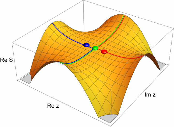
The analog of Rayleigh-Schrödinger perturbation theory in the 0D case is the perturbative expansion of . Because the action has 3 saddle points, two minima at and a local maximum at , there are 3 different series expansions we can compute. For the saddles at , setting and expanding gives
| (3.8) |
This is an ordinary series, up to the overall factor of , which is a normalization convention. It is asymptotic with coefficients that are factorially divergent as .
The saddle-point approximation around is a little different. First of all, at the action is nonzero. This leads to a non-perturbative factor multiplying each term in the saddle-point approximation. Since is a local maximum, increases in the imaginary direction, not in the real direction, so we must expand along . The choice of sign is arbitrary. The result is then a trans-series:
| (3.9) |
This series is also asymptotic, with the coefficients growing as at large , but now alternating in sign. This is a general phenomenon, as we will see, at the heart of resurgence: saddle points with higher action give alternating-sign series, and those with lower action give non-alternating series.
The key to combining these separate expansions into the full trans-series and then reconstructing the non-perturbative function is to use the Borel transform, as introduced in Section 3.1. Since the original contour can be decomposed into a sum of thimbles, the exact answer is recovered by summing the Borel resummations of all contributing saddles. In our case, the integration contours used in the saddle-point expansions are straight lines – along the real axis for and the imaginary axis for . However, the Lefschetz thimbles (steepest descent trajectories) labeled are not linear. These can be seen in Fig. 2. By observation, the original real contour can be seen to be a concatenation of these Lefschetz thimble paths:
| (3.10) |
The exact integral is then
| (3.11) |
with intersection numbers . The exact integral can be recovered from the series expansions by
| (3.12) |
where denotes Borel resummation and
| (3.13) |
is the full trans-series. The sign ambiguity arises from a choice of contour deformation to avoid the Stokes point at where the thimbles intersect.
To verify that this procedure is correct, we next explicitly compute the Borel transforms and resummations for the separate saddle point expansions and verify that their sum reproduces the full non-perturbative function. The Borel transform of the series in Eq. (3.8) is
| (3.14) |
This has a branch point at , corresponding to the action at the unstable saddle. The lateral Borel resummation is
| (3.15) |
where indicates deforming the contour above (+) or below () the branch cut starting at . This integral can be evaluated by changing variables to , giving
| (3.16) |
We can confirm this by direct integration along the Lefschetz thimble . As shown in Fig. 2, the thimble through runs from along the real axis to the origin, then down to along the imaginary axis. Parametrizing the contour piecewise with for and for :
| (3.17) |
These integrals can be evaluated using the substitutions and , yielding Bessel functions. The result is
| (3.18) |
which, after using the identity , confirms the equivalence between Borel resummation and thimble integration. Note that the choice of is related to the choice of contour deformation in Eq. (3.15). If we deform the contour below the branch cut, we would instead curve up to in the complex plane. The analysis of the saddle at is similar, but the thimble approaches the origin from the opposite side. Explicitly,
| (3.19) |
For Eq. (3.9) the Borel transform is
| (3.20) |
This has no singularity on the positive real axis, so Borel resummation is unambiguous:
| (3.21) |
This can also be verified by direct integration along the thimble , which runs along the imaginary axis from to , where the orientation is again defined by the choice of sign in Eq. (3.20):
| (3.22) |
Finally, we confirm that the sum reproduces the exact function. Adding the contributions, the two minima contribute the functions along with an imaginary , while the unstable saddle contributes a compensating imaginary such that the sum of all thimbles reproduces Eq. (3.7). The imaginary ambiguity from reflects that different choices of thimble orientation give results differing by exponentially small imaginary terms that cancel in physical observables.
This zero-dimensional example illustrates the key features that will reappear in the quantum mechanical double well: (i) multiple saddle points with different actions, (ii) asymptotic series around each saddle whose Borel transforms have singularities at the actions of other saddles, (iii) reconstruction of the exact answer through thimble decomposition, and (iv) cancellation of imaginary ambiguities between different saddle contributions.
3.3 Alien calculus and resurgence
We saw in the double well that the full path integral can be reconstructed by combining the asymptotic series around each saddle separately. That the imaginary parts must cancel implies that these series are not completely independent. A central idea of resurgence is that you can actually reconstruct the full function from the expansion around a single saddle. The general framework for doing this is alien calculus, developed by Écalle [46, 47, 48]. For pedagogical introductions, see the reviews by Sauzin [89], Dorigoni [40], and Aniceto, Başar, and Schiappa [8].
The key object is the alien derivative , which extracts information about singularities of the Borel transform at . For a function with Borel transform , the alien derivative at measures the discontinuity across the branch cut starting at :
| (3.23) |
More precisely, for a “simple” resurgent function the Borel transform has the local form
| (3.24) |
with analytic at (the minor). The alien derivative is then defined by : it strips off the logarithmic branch and returns the analytic coefficient. Since , this is equivalent to the recentered discontinuity .
For the 0D double well, consider again the perturbative series around from Eq. (3.8). Its Borel transform has a branch point at . Near this singularity:
| (3.25) |
The discontinuity across the branch cut for is
| (3.26) |
Remarkably, this is precisely the expression in Eq. (3.20). That is,
| (3.27) |
This is the resurgence relation: the discontinuity of the perturbative Borel transform at the instanton action encodes the instanton series itself. In the alien-calculus language above, the shift is built into , so this reads:
| (3.28) |
The alien derivative is directly connected to the Lefschetz thimble picture. When performing lateral Borel resummation versus (integrating above or below a singularity), the difference corresponds to picking up the thimble associated with the saddle at action :
| (3.29) |
Thus the alien derivative gives the Stokes constant—the coefficient with which the thimble contributes when crossing a Stokes line. Alien calculus provides an algebraic way to compute the intersection numbers directly from the singularity structure of the Borel transform, without explicitly constructing the thimbles.
The full trans-series can now be reconstructed iteratively. Starting from alone:
- 1.
The Borel singularity at reveals the instanton action .
- 2.
The alien derivative gives the instanton series.
- 3.
Since has no singularities on the positive real axis, there are no further alien derivatives to compute.
The full answer is then
| (3.30) |
where requires no lateral choice since has no singularities on the positive real axis. For either choice of lateral resummation, and each acquire imaginary contributions from the Borel singularity at , which cancel exactly against , ensuring the total partition function is real.
This demonstrates the key insight of resurgence: perturbation theory is not merely incomplete, it contains hidden information about the full non-perturbative structure of the theory. The divergent tail of the perturbative series, which grows as , encodes the locations and contributions of non-perturbative saddles. From the Borel transform of a single asymptotic expansion, one can in principle reconstruct the entire trans-series and thereby obtain a non-perturbative definition of the theory.
3.4 Action-Borel correspondence
For the 0D double well, there is an alternative and more direct way to reconstruct the full function from a single saddle, using the Action-Borel correspondence introduced in [25]. The basic idea is that if we have a function defined through an action
| (3.31) |
with , then we can compute the Borel transform through a change of variables. Writing
| (3.32) |
we can read off the Borel transform as
| (3.33) |
This manipulation identifies the Borel variable with the action . Integrating and using the fact that , we find that in one dimension
| (3.34) |
where the sum is over all roots of and the signs are . This correspondence is therefore a duality: not only is the Borel variable equal to the action, but the action variable equals the Borel transform. Some examples can be found in [25]. Singularities in arise precisely at the critical values of —the saddle point actions—providing a direct geometric interpretation of Borel singularities.
The power of this correspondence is that it works in reverse: given the Borel transform, we can reconstruct the action. To see how this works for the double well, suppose we only have the asymptotic series (or ) around one of the minima, as in Eq. (3.8). Its Borel transform is in Eq. (3.14), and from its discontinuity we can reconstruct the Borel transform of as . In the region we recover the full Borel transform by adding . Anticipating two domains for a stable action we can solve and recover , which is the correct action. In this way, we can reconstruct the full function from the perturbative expansion around a single saddle, providing a concrete realization of the resurgence program.
3.5 Riemann surface picture
The different Borel transforms arising from the different asymptotic expansions around the different saddle points are not independent. They are different branches of a single Borel transform which naturally lives on a Riemann surface. For the double well, the action is
| (3.35) |
Mapping and according to the action-Borel correspondence, we then see that the Borel transform is a multi-valued function on a 4-sheeted Riemann surface defined by
| (3.36) |
Solving gives the four branches,
| (3.37) |
numbered from bottom to top at . The plot shows just the real parts of the four branches: the Borel transforms become imaginary at the branch points. These four sheets describe the Riemann surface over the -plane, with branch points at the critical values of . At , sheets 1 and 2 and sheets 3 and 4 coalesce, while at , sheets 2 and 3 coalesce. The four branches are related by analytic continuation around the branch points: and around , and around . Figure 3 shows the full Riemann surface in three dimensions, with the two steepest-ascent arms of the thimble traced in cyan.
At a saddle the steepest descent contour follows the two directions along which increases away from . These two arms correspond to the two sheets that coalesce at . Under the change of variables , both arms map to the same ray , but with opposite orientations: the contour first traverses one arm from inward to , passes through the saddle, and then traverses the other arm from outward to . Re-parametrising both arms by increasing , the inward-traversed arm acquires a sign reversal, giving
| (3.38) |
Integrating by parts, the boundary terms vanish (at , and at the exponential goes to zero). This gives
| (3.39) | ||||
| (3.40) |
where we shifted in the second step. From here, we can read off that the Borel transform is . This is the same Borel transform computed from the asymptotic series around the saddle.
To check, consider the minima at where . At this point sheets and coalesce and so
| (3.41) |
From the explicit formulas in Eq. (3.37)
| (3.42) |
which is precisely from Eq. (3.14): the Borel transform of the series is the difference of the two coalescing branches.
For the unstable saddle at we have and sheets 2 and 3 coalesce there. In this case,
| (3.43) |
and
| (3.44) |
which matches Eq. (3.20).
4 Exact WKB
Although the simple double well integral in Section 3 demonstrates the basic principles of resurgence, to compute the trans-series in quantum mechanics requires significantly more sophisticated methodology. In this section, the Exact WKB method is discussed. Section 5 discusses the complementary path integral approach.
In the WKB method, the energy levels of a particle in a double-well potential are quantized by demanding the wavefunction be normalizable, dying off exponentially both as and . If we want to compute an approximate solution, we could start from large where the solution to the Schrödinger equation should be of the form which is exponentially small, with zero admixture of the complementary solution. If we then analytically continue this form to large negative we still have which is now exponentially growing as . On the other hand, energy eigenstates for a polynomial potential must be smooth (in fact ) functions. The way to reconcile these two behaviors involves understanding asymptotic expansions: it is possible for a function to be analytic around with an infinite radius of convergence, but to have asymptotic expansions that change abruptly at . A simple example is . Its asymptotic behavior for is while its behavior as is . The transition is along a line in the complex plane where . More generally the region of the complex plane where the asymptotic expansion abruptly changes is called a Stokes line.
In quantum mechanics, we can take any potential and expand locally around a turning point where . Then is linear. Thus, near a turning point the Schrödinger equation reduces to Airy’s equation
| (4.1) |
The two independent solutions to this equation are and which are analytic functions, being the solution which decays exponentially at large , while grows exponentially. These Airy functions, like , are analytic around with an infinite radius of convergence, but have asymptotic expansions at whose form changes abruptly for certain values of . So to overcome the challenge with WKB, matching across turning points analytically while imposing asymptotic boundary conditions, we begin with a thorough exploration of Airy functions and the associated identification of the relevant Stokes lines.
4.1 Airy functions
The most familiar place where Airy functions appear in nature is the rainbow. When sunlight scatters off water droplets in the atmosphere, most of the light is scattered in random directions. However, at certain special angles, many rays pile up, creating a bright caustic—the rainbow. For a single water droplet, classical ray optics predicts that light entering at impact parameter scatters at deflection angle . The deflection function has an extremum at the rainbow angle where . At this angle, an infinite number of nearby rays pile up, leading to a divergence in the classical cross section.
This problem was first investigated systematically by George Biddell Airy in 1838 [4] (see also [77] for a modern account), who sought to explain the supernumerary bows—faint colored fringes appearing just inside the primary rainbow. Airy recognized that the classical geometric optics prediction breaks down near the caustic and that one must account for the wave nature of light. Near the rainbow angle, the wavefront emerging from the droplet acquires a cubic shape: in coordinates aligned with the caustic ray, the wavefront is approximately for some constant . Applying Huygens’ principle, the amplitude at observation angle relative to the caustic ray is obtained by integrating the secondary-wave contributions along the wavefront. The path difference to the observer from a point at position on the wavefront is for small angles, so the amplitude is
| (4.2) |
Rescaling and defining , this becomes
| (4.3) |
The parameter is proportional to the deviation from the rainbow angle, so the intensity is
| (4.4) |
This formula predicts not only the bright primary rainbow but also the supernumerary bows: the oscillations of for correspond to alternating bright and dark fringes just inside the main bow, as shown in Fig. 4. These oscillations are precisely analogous to the quantum mechanical oscillations that occur in the classically allowed region of a potential well. The characteristic behavior of the Airy function – oscillations for and exponential decay for – directly maps to the bright rainbow and the dark region beyond it.
The series expansion of the Airy function is
| (4.5) |
which is convergent for all . We can also write
| (4.6) |
where is a modified Bessel function of the second kind. The asymptotic expansions of for large positive and negative are
| (4.7) |
As expected from our quantum mechanics intuition, the Airy function transitions from exponential behavior in the forbidden region of the linear potential barrier, where on the right side of the barrier, to oscillatory behavior, when for .
The other independent solution to Airy’s equation, Eq. (4.1), is , which can be written as
| (4.8) |
where is a modified Bessel function of the first kind. Like , the function also transitions between exponential and oscillatory behavior, but with opposite character:
| (4.9) |
For , grows exponentially while decays; for , both oscillate but with a phase difference.
To understand the change in the form of the asymptotic expansion of it is helpful to explore its integral representation, cf. Eq. (4.3), extended to complex values as
| (4.10) |
where
| (4.11) |
and is the Airy integration contour22 2 We are free to deform this contour as we desire, provided that the end points remain in the same convergent regions. In particular, for small values we only need to slightly curve the real line. that goes between the asymptotic regions as . This way of writing is very powerful, since the analytic continuation is simple: just do the integral with different values of . Note that because of the behavior of the action at large the integral is convergent within 3 wedges and of angular size in the complex plane centered on and :
| (4.12) |
If we consider more generally integrals defined by a contour
| (4.13) |
then the contours fall into one of 6 relative homology classes, determined only by which two distinct regions or the integral starts and ends in. Any contour going between the same boundary regions gives the same result. At real the Airy function has an integration contour along the real line which is just barely integrable, as its endpoints are on the boundary of the allowed asymptotic region. For complex values we need to slightly curve the real line so that it starts and ends in the convergent regions and respectively (see Fig. 5). So in general we have
| (4.14) |
The other two independent contour integrals give linear combinations of and :
| (4.15) |
Thus,
| (4.16) |
Note that is a sum of two contours that both end at , so they cannot be joined into a single contour.
4.2 Stokes lines
The integral representation allows us to determine the asymptotic behavior. The Airy integrand is highly oscillatory except near saddle points, so its dominant behavior will be determined by the points of stationary phase. For the Airy action, these are at with action and behavior . As is moved around in , these saddle points move around as well, switching places when the branch cut, conventionally placed on the negative real line, is crossed. If we avoid the branch cut with there are then two well-defined integrals, defined not through asymptotically convergent regions but rather as thimbles, steepest-descent trajectories passing through the saddles. For these integrals give in the saddle point approximation
| (4.17) | ||||
| (4.18) |
where
| (4.19) |
Note that is real for real , while is purely imaginary for real . The subscript in refers to the saddle point location , which is opposite to the sign of the exponent .
To see which asymptotic behavior applies for which integral we need to decompose into a concatenation of thimbles. For any fixed , each thimble belongs to one of the 6 relative homology classes. However, unlike the Airy contour which is always defined as , which class the thimble is in depends on the phase of . Thimbles for different phases are shown in the bottom panels of Fig. 5. We can then see, for example, that for real , the Airy contour is the same as the thimble passing through , so its asymptotic expansion is . However, as the phase of passes we find that neither thimble goes between anymore. Instead, the Airy contour follows an thimble and then . Then the asymptotic behavior of Ai in this region will be given by the sum which is oscillatory.
In an asymptotic expansion, only the leading asymptotic behavior is kept. Which behavior dominates is determined by the sign of . On a Stokes line, the real part of the two asymptotic forms is maximally different. The domains between Stokes lines are called Stokes regions. For the Airy integral, we sketch the Stokes lines as
| (4.20) |
The solid lines are the Stokes lines at , and the wavy line is the branch cut at . These Stokes lines are in the complex plane and the or indicate which asymptotic expansion applies exclusively when along that line. At (positive real ), so grows, meaning is dominant. At , is real and negative, so grows, meaning is dominant. Note that here are a convention with no physical meaning.

Now let us return to the quantum mechanics problem where we have a potential barrier at , with the forbidden region and the allowed region. We want to match from a function which is exponentially decaying for across the barrier. So in the region the function should be , which is the green contour in either of the middle two panels of Fig. 5. There cannot be any admixture of for it to be normalizable. As we analytically continue past the thimble flips asymptotic regions. This means that a well-defined integral such as that had a component of will now have the sum of and , which, as we observed, becomes oscillatory. This is the expected behavior in the classically allowed region. If we had started with instead, which matches onto the thimble in the region, then since the thimble does not flip when the Stokes line is crossed, its asymptotic expansion also does not change.
To determine how the asymptotic behavior changes across Stokes lines more systematically, suppose we have some physical33 3 Here physical means defined by an integral like a path integral with a fixed contour or a differential equation with boundary conditions, in contrast to being defined through a perturbative expansion, which would be associated with a thimble and a saddle point. function like or a wavefunction, or a path integral. In any asymptotic region, we can write where are integrals along thimbles. This decomposition is local, applying near any turning point (the linear potential giving rise to the Airy integral only has one turning point; the multiple turning point case will be considered shortly). Then as is analytically continued across a Stokes line, the thimbles may get associated with different asymptotically convergent regions. Then the coefficients will change. For example, with the Airy function we observed that if to begin with, on the other side of the Stokes line it is . With , which corresponds to , when the same Stokes line is crossed, it doesn’t change. Combining these observations, we conclude that when crossing the Stokes line counterclockwise the asymptotic behavior changes according to where
| (4.21) |
One can check that the same behavior occurs when crossing the other Stokes line at . When traversing a Stokes line, the corresponding matrix is44 4 Some references, e.g. [97, 30], exhibit connection matrices with an extra factor of in the off-diagonal terms. This stems from a convention that the asymptotic expansions are real. Our convention instead treats the two saddle-point contributions on the same footing — each is the integral over its thimble with no relative phase inserted by hand.
| (4.22) |
These matrices are known as connection matrices (or Stokes matrices). When crossing a Stokes line clockwise around the turning point, the matrices are invoked.
For the Airy function, with our convention, the branch cut is at on the principal sheet. Traversing it counterclockwise corresponds to moving from the 6th panel in Fig. 5 to the first, whereby the thimble becomes the thimble and the thimble becomes the thimble with opposite orientation. We can represent this transition with the connection matrix
| (4.23) |
This is a rotation matrix. As a check, referring back to the diagram in Eq. (4.20) and the Fig. 5, if we go in a full circle, we pick up a trivial monodromy , confirming that analytic continuation is self-consistent (or providing an alternative way to compute ).
For an example use of these automorphisms, let’s use them to continue the Airy function from positive real to negative real . For positive , we want exponential damping only so that the asymptotic expansion of must be , so as before. Note that crossing the Stokes line does nothing at , so it doesn’t matter if we had started above or below the real axis. We then analytically continue counterclockwise. When we cross the Stokes line at we get . This form holds until the negative real axis. Thus, when we get to , we have . Combining the two exponentials with the phase shift gives the oscillatory asymptotic expansion of the Airy function:
| (4.24) |
In this way we have analytically continued a function from the forbidden region to the allowed region avoiding the turning point at . Note that although we have placed the branch cut at , we can either push it out of the way when we get there, or cross it. Crossing it gives . Although Ai is an analytic function, this sign flip correctly accounts for its asymptotic expansion for below the negative real axis.
In summary, the Stokes automorphisms allow us to track the abrupt changes in the asymptotic expansion of a function as a Stokes line is crossed. As we noted, on a Stokes line one asymptotic expansion is maximally dominant over the other. As the Stokes line is crossed, the subdominant component picks up an admixture of the dominant component, but the dominant component does not change. For instance crossing the Stokes line where dominates takes us from . This arrangement is in a sense minimally disruptive: the mixing occurs where the smallest possible contribution is added to the maximum possible contribution. We have presented the discussion of Stokes automorphisms without mentioning Borel resummation. However, as we discuss next, this is the same phenomenon seen in lateral Borel resummation: as the integration contour is continued across a branch cut in the Borel plane, the resummed expression picks up an exponentially subdominant contribution.
4.3 Stokes automorphisms in the Borel plane
Recall from Section 3.5 that there is a natural way to interpret saddle points of the action as branch points of a Riemann surface. In this picture, thimbles move along the Riemann surface, passing from one sheet to another at the branch point. The Riemann surface picture connects the Borel transform and the action. In the Airy case, we first rescale the coordinates so the Borel transform is easier to see, then we use the geometric Riemann-surface picture to connect the Stokes matrices to lateral Borel resummation.
As discussed above, both the Airy function and the thimble integrals are defined by the same integrand with ; they differ only in the choice of contour. Changing variables to and defining , these integrals then have the form
| (4.25) |
where the rescaled action is
| (4.26) |
This action has critical points at with critical values .
Following the same procedure as for the zero-dimensional double well (Section 3.5), we identify the Borel transform as the multi-valued inverse of the action:
| (4.27) |
This equation describes a three-sheeted Riemann surface over the -plane, as shown in Fig. 6. The branches are
| (4.28) |
labeled from bottom to top at . Beyond the branch points at , two of the three branches become complex conjugates; their real parts (solid) are slightly displaced for clarity, and their imaginary parts are shown as dotted lines. For we take the continuation from such that and ; for the roles of are analogous. The branches coalesce at the critical values of : at and at . The three branches are related by analytic continuation: around and around .55 5 The three branches are related by for all , which follows from Vieta’s formulas for the sum of the roots of a cubic polynomial. Sewing together the different sheets as shown in Fig. 6 gives a concrete realization of the action–Borel correspondence of Eq. (3.34): the Borel variable is the action, and is the field configuration.
Now consider the thimble integrals. The integral is defined along the thimble passing through . Just as in Section 3.5, the thimble has two arms meeting at the saddle. Here we see that at , sheets 2 and 3 coalesce, so one arm lives on sheet 2 and the other on sheet 3. Changing variables from to , the measure on each arm is , and the two arms contribute with opposite orientations. So we can write for real positive
| (4.29) |
Integrating by parts, the boundary terms vanish. Then we get
| (4.30) | ||||
| (4.31) |
where we shifted in the second step. We can then read off the Borel transform: . Note that is the discontinuity across the branch cut of the Riemann surface where sheets 2 and 3 coalesce. Since the integrand is single-valued for there is no ambiguity and the integrand is regular at . The Borel transform for does have a singularity inherited from the other branch point of : the point where sheets 1 and 2 meet, which maps to in the shifted variable. This singularity lies behind the contour (on the negative real axis), so is Borel summable and no tilting of the integration contour is required. Indeed for positive we can verify that the series defined in Eq. (4.17) is factorially growing, but sign-alternating, and hence Borel summable.
A similar computation applies for , where sheets 1 and 2 coalesce at . The integrand is now the discontinuity across the cut at :
| (4.32) |
We can again read off the Borel transform: . In this case, the integrand is single-valued along its own cut ( in these variables), but now the other branch point —where sheets 2 and 3 meet, or in the shifted variable—sits directly on the positive real integration ray. For this reason we had to deform the integration contour, tilting off the real axis, to go to . Going above or below the branch point gives different analytic continuations, so the integral is ambiguous: the tilt passes above the cut, giving the lateral Borel resummation , while passes below, giving . This ambiguity in the lateral Borel resummation is reflected in the fact that the series of Eq. (4.18) is factorially growing and non sign-alternating. The monodromy around the obstructing branch point at swaps while leaving unchanged, so the jump of the integrand across the cut is : minus the combination that defines . The two lateral Borel sums therefore differ by a contour integral encircling this branch point, giving the Stokes relation
| (4.33) |
with the Stokes constant (which equals the entry of the connection matrix ) determined by the monodromy exponent at the square-root branch point.
This is the simplest instance of the Delabaere–Dillinger–Pham (DDP) formula [39, 36]: the discontinuity of one Borel-resummed quantity across a Stokes line is controlled by another. This structure generalizes: whenever a problem has resurgent Borel singularities, the discontinuity across a Stokes line at distance is proportional to times another quantity. We will see the same pattern for the double-well in Section 4.6.
The DDP formula is often repackaged into a Stokes automorphism operator
| (4.34) |
acting on trans-series. This operator encodes the monodromy of a formal series around the Borel branch point: integrates above the singularity, below, so is the analytic continuation around it. Using that is Borel summable, so , and Eq. (4.33), we then have
| (4.35) |
Both and are determined by the same Stokes constant, so it’s natural that they are related. But it’s important to emphasize that they act on different objects: acts on the formal asymptotic series themselves, while acts on the coefficient vectors that specify how much of each series appears in a physical solution. In quantum mechanics, will remain a matrix but as an operator will act on the much larger space of trans-series.66 6 For the Airy function (a one-dimensional integral with two saddle points), is completely captured by a matrix and carries the same information as . In quantum mechanics the situation is richer: the quantum-mechanical trans-series contains infinitely many multi-instanton sectors, and acts on this entire infinite-dimensional graded space via Écalle’s formula (Eq. (4.140)). The connection matrix remains finite-dimensional, acting on the two WKB solutions with entries that become functions of the Voros symbols (Eq. (4.72)). Thus resolves the sector-by-sector resurgent structure, while summarizes only the net Stokes jump of the wave function.

Now are defined as thimble integrals in space. In -space these saddles originate at the branch points at and move in steepest ascent trajectories of the action where is maximized, i.e. along straight lines defined by . The lowest real-action point along the trajectories is at the saddle, so these thimbles have the asymptotic expansion for any . For real positive , has lower action (the 1-2 branch point on the Riemann surface is lower) and the curve moves upward until it hits the branch point. That is why has a discontinuity and does not. This is general: the dominant saddle (smaller action at the saddle point) has an ambiguity given by directing its contour above or below the second saddle it hits. As is continued, the lines associated with the thimbles rotate around. At the anti-Stokes line (where the real parts of the two asymptotic exponents are equal), (), the two contributions have equal magnitude and at the Stokes line () they have switched places. These contours are shown in Fig. 7 for various choices of . Each thimble has two arms meeting at the saddle; these two arms live on different sheets of the Riemann surface but project onto the same curve in the -plane. A curve emanating from a branch point along which two sheets coalesce is precisely a branch cut. Thus the thimble images define a natural, -dependent choice of branch cuts emanating from .
In contrast to which are pinned to saddles, the contour associated with the Airy function is a fixed contour in space going between convergent regions and . Since , the Borel variable is related to the original integration variable by
| (4.36) |
For the Airy contour in space can be taken as a slight deformation of the real line, as seen in the first panel of Fig. 5. From Eq. (4.36) we can see that this will map in space into a contour that is a slight deformation of the imaginary axis. The Borel integral is convergent for , so we can deform this contour to a Hankel contour encircling the branch point, where sheets 2 and 3 meet. With the chosen orientation, this picks up the discontinuity across the cut, which is exactly the integrand of . This gives for real positive , recovering the standard result. As we rotate clockwise, the Airy contour (real ) deforms according to Eq. (4.36). Its image in the plane is shown in Fig. 7 for some values of . We see that it always avoids the branch points, as it must since is analytic. The Stokes phenomenon occurs precisely when a thimble contour passes the subleading saddle, which discontinuously changes the decomposition of the Airy contour’s image into thimbles.
The Borel transforms we have derived also determine the asymptotic behavior of . Writing
| (4.37) |
the coefficients and are determined by the Taylor expansion of the respective Borel transforms around . For , the Borel transform is . This combination passes smoothly between sheets 2 and 3 at their coalescence point (i.e. before shifting), so it is not singular there. The only singularity of this Borel transform is at , the other branch point where sheets 1 and 2 meet. Its Taylor coefficients therefore scale as , giving . For , the Borel transform is similarly regular at its own branch point ; its only singularity is at (where sheets 2 and 3 meet), giving with constant sign:
| (4.38) |
Recalling we have
| (4.39) |
reproducing the asymptotic form of the series in Eqs. (4.17)–(4.18). The alternating signs for and constant signs for reflect the Borel singularity lying on the negative and positive real axes respectively.
Since the Borel singularity of sits on the positive real integration ray, is not Borel summable: the lateral resummations differ by the discontinuity across the cut at . But this is exactly the content of the DDP relation, Eq. (4.33): . Since is purely imaginary for real , the two lateral resummations have the same imaginary part but different real parts:
| (4.40) |
The real ambiguity of the dominant saddle (, with its non-alternating series) is exactly . Since , the ambiguity is suppressed relative to by , the exponential of the difference of the two saddle-point actions.
4.4 Exact WKB
In this section and onward, we use natural units throughout where the potential is taken to be a function, the mass is set to unity and the perturbation expansion is done in terms of .
The WKB expansion begins by approximating a wavefunction as the exponential of the action: . Plugging this WKB Ansatz into the Schrödinger equation with gives
| (4.41) |
In the limit this is the Hamilton-Jacobi equation satisfied by the classical action . The corrections to the phase correspond to including non-classical paths in the path integral. In the Hamilton-Jacobi equation one normally identifies with the classical momentum . In the treatments of Exact WKB it is conventional to include a factor of , so . Either way, the action is (up to a factor of ) an integral over . Introducing the energy as an integration constant, the WKB Ansatz is then
| (4.42) |
and the Schrödinger equation becomes
| (4.43) |
This nonlinear differential equation is an example of a Riccati equation. It can be solved iteratively in perturbation theory.
At the solution to Eq. (4.43) is
| (4.44) |
which is times the classical momentum of a particle with energy in a potential . Thus, is real in forbidden regions and imaginary in allowed regions. For the corrections, we write and solve perturbatively in . The perturbation expansion can be written as a recursion relation
| (4.45) |
In particular, once a sign is chosen for , all of the higher-order terms are completely fixed. For example, the next few terms are
| (4.46) | ||||
| (4.47) | ||||
| (4.48) |
and so on.
For polynomial potentials, the spectral curve is algebraic, and each is a rational function of and . For the quartic double well, this curve is elliptic (genus 1), and and span its first cohomology. The differential can therefore be decomposed as
| (4.49) |
where and depend only on (and the potential), and is single-valued so that integrates to zero around any closed cycle. For other potentials, the spectral curve can have higher genus and additional basis differentials would be needed. In practice, the decomposition is constructed by writing where is a polynomial and is an integer, making an ansatz with an undetermined polynomial, and matching coefficients to solve for , , and . For example, is already a total derivative, so and . The coefficients and are potential-dependent and will be computed explicitly for the double well in Section 4.7, while additional details are left to Appendix B.
One simplifying feature of the recursion is that only the terms with even depend on the sign choice for . To see this, we write
| (4.50) |
where
| (4.51) | ||||
| (4.52) |
Then the terms with odd powers of in the Riccati equation are
| (4.53) |
from which we deduce that independent of the sign. Since is a derivative its contribution to can be integrated allowing us to write the wavefunction as
| (4.54) |
up to normalization. In summary, we can determine the WKB wavefunction perturbatively using the even terms, which can be computed recursively.
The leading WKB expansion takes . At the turning points, and blows up. The Exact WKB approach analytically continues around this singular region. To proceed, consider taking close to a turning point at . Then and
| (4.55) |
Here we recognize the asymptotic expansion of the Airy function, Eq. (4.7), upon identifying . The -independent prefactors only affect the normalization, but are different for the solutions. Rather than keep track of these normalization factors, it is simpler to absorb them into the integral by adjusting the (arbitrary) basepoint of integration from to the turning point . That is, we define
| (4.56) |
as the two branches associated with turning point , located at . To track the normalization change between two turning points and , we note that
| (4.57) |
where
| (4.58) |
is known as a Voros symbol. We can then account for the change in normalization moving from to with a connection matrix , acting on the coefficient vector in
| (4.59) |
The Voros symbol involves a period integral between two turning points where has algebraic branch points. For example, the harmonic oscillator potential is . For this potential, which has two branch points at . To get the expected oscillatory behavior in the classically allowed region where , between the turning points, we would like to be imaginary there. Analytic continuation from positive to negative real goes counterclockwise through the upper half of the complex -plane, avoiding the branch points. This then lets us write the Voros symbol as a monodromy around the branch points:
| (4.60) |
The integral is along a closed contour encircling counterclockwise the two branch points surrounding a classically allowed region. It is convenient to also introduce which we denote by . So, in Eq. (4.59) is to be used when going from to above the branch cut if , but is used when going below the branch cut (or above the branch cut from ). For two turning points surrounding a forbidden region, the integrand is real and so is used (there is no branch cut). An alternative convention is to have the branch cuts go from each turning point off to infinity, as shown on the left in Fig. 8. Then one uses the branch-cut Stokes automorphism, Eq. (4.23), in the analytic continuation when crossing each branch cut.
4.5 Warm up: simple harmonic oscillator
As a warm-up computation with Exact WKB, we consider the harmonic oscillator with . The turning points are :
| (4.61) |
The goal is then to analytically continue from the far right to the far left along the arc as shown. We will do this by using connection matrices where we can quantize the energies by demanding exponential decay as . To construct the Stokes diagram for this potential, we start on the right close to the turning point where the potential grows linearly like the Airy potential. On the left, the potential also grows, and this can be represented with its own Airy Stokes diagram. To connect them, we can either join the branch cuts or point them in complex conjugate directions. The result is shown in Fig. 8, where the and labels indicate the Stokes lines where the functions and from Eq. (4.55) are respectively subdominant, consistent with the branch cut choice.
We begin at large real where we want to be exponentially decaying. Writing with defined by Eq. (4.55), the decaying contribution at large positive is , so the boundary condition selects . The connection matrices from Section 4.2 were constructed with the decaying-mode coefficient in the first slot of ; to reuse them here we order the vector as , and the starting point is . Note that, as with the Airy function, it doesn’t matter if we start at large above or below the Stokes line, since . Moving counterclockwise, we first cross a Stokes line and get . With both components turned on the wavefunction is oscillatory, as expected between the turning points. To get to the next turning point, we must use a Voros connection to adjust the normalization. Then we cross a branch cut from the left region and finally another Stokes line to get to the asymptotically region. The result is that on the far left
| (4.62) |
For , we need the wavefunction to decay, which means the exponentially growing component must be absent. This requires which means the first entry must vanish and therefore
| (4.63) |
As a cross-check that we got the right condition, note that the first entry of doesn’t change as we cross the Stokes line at negative , since leaves the first entry invariant. Therefore our quantization condition for the harmonic oscillator is independent of our location above or below the Stokes line at negative real and reads
| (4.64) |
To solve this for we first compute the even terms in the momentum expansion:
| (4.65) |
In general, at large . This means that if we deform the contour of integration in the Voros symbol to be large, then all the with will not contribute. The contour integral over does not vanish; it gives . Therefore . These are exactly the correct energies for the simple harmonic oscillator.
As an additional cross check, we can consider continuing our wavefunction all the way around a counterclockwise circle back to the positive real region. If we use the configuration on the left in Fig. 8, where the branch points go to infinity, the connection formula using the appropriate branch cuts and continuations is
| (4.66) |
This monodromy check verifies the consistency of the sign choices and connection matrices. If instead we use the configuration on the right in Fig. 8, where the branch points are merged, we get the appropriate connection formula as
| (4.67) |
To understand why this gives instead of , consider the contour integral around a path encircling branch points at . With a branch cut between the turning points, we can deform this to an integral along the cut, giving , not zero. The non-zero result reflects the fact that the Stokes diagram with a shared branch cut does not fully account for all phase accumulation. This point is clearly articulated in [30]. Additional examples can also be found in [97].
4.6 Double well
For the double well, the basic procedure is the same as the harmonic oscillator, but a few complications arise. We use a double-well potential normalized as
| (4.68) |
This potential has minima at and a local maximum at . We choose for the normalization so that for the harmonic oscillator at each minimum. For energy the turning points are at
| (4.69) |
We are primarily interested in the low-energy spectrum where so that tunneling is relevant. States with are above the barrier.
The potential and associated Stokes graph are
| (4.70) |
In this case, in addition to the branch cuts intersecting, the Stokes lines intersect. One of the Stokes lines from appears on top of one of the Stokes lines from . These intersections of Stokes lines give a Stokes phenomenon similar to what we saw in the double well in Section 3 where the thimbles intersect. It occurs because there is a non-alternating series leading to a singularity on the positive Borel axis. The ambiguity can be resolved by giving a small imaginary piece to . Depending on the sign of this deformation the Stokes lines will deform upwards or downwards. We also deform the branch cuts to resolve their intersection, as we did in Fig. 8. The resulting Stokes graph for one sign choice is shown in Fig. 9. As a consistency check, extending the path in Fig. 9 to a full monodromy gives
| (4.71) |
as expected.
To impose the asymptotic boundary conditions, we proceed as with the simple harmonic oscillator example. We begin with in the region. The combined connection formula to the negative region is
| (4.72) |
where the perturbative and non-perturbative Voros symbols are
| (4.73) |
The contour goes counterclockwise around and (or around and ), while goes counterclockwise around and . Although the contour passes through the branch cuts, the discontinuities cancel and the exponent in equals minus twice the integral of between the two turning points divided by . The Voros symbol is the Exact WKB generalization of the WKB tunneling amplitude.
The quantization condition we need is where as in the SHO example. This implies
| (4.74) |
which is the quantization condition for the double well.
Before solving this quantization condition, we note that the double well is invariant under , so the energy eigenstates will be parity eigenstates. The parity odd states will have and the parity even ones will have . If a wavefunction is even or odd, then the boundary conditions at are determined by those at . This observation allows us to replace the boundary condition at with one imposing or . To evaluate we can continue the function from the asymptotic region to the middle region between the and Stokes lines using . Then the wavefunction in this region is
| (4.75) |
Noting that involves an integral from to which is of the integral in the exponent of , and accounting for the continuation of the square-root prefactor of the branch around the turning point, we can write, up to an overall normalization,
| (4.76) |
This allows us to evaluate by starting from in the large region, continuing to the central region, and contracting with :
| (4.77) |
which leads to
| (4.78) |
Imposing for the even states rather than adds a minus sign to the lower component so that,
| (4.79) |
These two quantization conditions for the even and odd parity wavefunctions are the two roots of Eq. (4.74).
If we had chosen instead, the line from would tilt upward and be crossed by the continuation path, while the line from would tilt downward and miss it, as shown in right panel of Fig. 9. This adds an extra to the chain to get to the middle region where lives. The odd-parity condition then reads
| (4.80) |
which gives
| (4.81) |
and the even condition gives
| (4.82) |
Since is imaginary in the allowed region (for real ), is a pure phase so that . Thus Eqs. (4.81) and (4.78) are complex conjugates of each other (as are Eqs. (4.79) and (4.82)) and give the same quantization condition for the real energies order by order in real .
Although the exponent in is imaginary for real at each order in perturbation theory, the resulting series at fixed is asymptotic. The overlapping Stokes lines between and for real , shown in Eq. (4.70), imply that is a non-alternating series and not Borel summable along the real axis; the two sign choices for correspond to two lateral Borel resummations which differ non-perturbatively. By contrast, ’s Stokes lines do not intersect and is Borel summable: both lateral sums agree, , and we simply write this common value as . Then Eqs. (4.81) and (4.78) become
| (4.83) | ||||
| (4.84) |
Multiplying Eq. (4.84) through by gives
| (4.85) |
Taking the difference between Eq. (4.83) and Eq. (4.85) gives
| (4.86) |
where Eq. (4.85) was used again in the second step. Acting with on both sides then gives the DDP relation for the double well77 7 To see that we use a foundational property of resurgence theory: the lateral Borel resummations are algebra morphisms, meaning they preserve products, . This follows because the Borel transform converts the ordinary product of formal series into the convolution product [89].
| (4.87) |
where is the Stokes automorphism defined in Eq. (4.34). Note that appears in Eq. (4.87), not : and are on the same footing as analytic objects on the Riemann surface of the Borel transform, and the is generated only by the parity quantization condition. In contrast to , the Stokes lines of lie at (set by being purely imaginary), away from the real axis, which is why is Borel summable:
| (4.88) |
i.e. .
4.7 Period integrals
In order to solve the quantization condition, we need to be able to compute the period integrals . At leading order and the integrals can be done in closed form. Let us write
| (4.91) |
with
| (4.92) |
Following convention, we call these “actions" even though they differ from the classical action by a factor of stemming from our convention introduced in Section 4. The leading-order perturbative action is
| (4.93) |
where and . This hypergeometric function has a convergent expansion at small , given by
| (4.94) |
where
| (4.95) |
The leading-order non-perturbative action is
| (4.96) | ||||
| (4.97) |
where .
The next period integrals we need involve which is computed using Eq. (4.47);
| (4.98) |
Trying to integrate this directly is more challenging than integrating . Even if we could do it, the subsequent integrals get harder and harder. Luckily there is a better way. After some algebra the differential can be written as
| (4.99) |
where
| (4.100) |
Integrated over the closed cycle (or ), the exact form drops out. So we have simply
| (4.101) |
and
| (4.102) |
In this way we get the next order without doing any additional elliptic integrals.
In fact, the same procedure works for all . Any can be written as
| (4.103) |
Then
| (4.104) |
with the Voros symbols following from Eq. (4.91). The reason this is possible is because the elliptic curve is genus one and its cohomology is two dimensional. This was discussed in Section 4.4 and a proof and algorithm to compute the and are given in Appendix B. We emphasize that to compute the and and hence to compute and requires no elliptic integrals, just some algebra. Explicitly,
| (4.105) | ||||
| (4.106) | ||||
| (4.107) |
and so on.
Inserting the expansions and expanding at small (anticipating that ) leads to
| (4.108) |
This is a perfectly sensible expansion where, at each order in , the individual series in converge for . Since the expansion reduces to a series expansion in . For the non-perturbative action, we find something different. The WKB expansion at small at each order in is
| (4.109) |
The inverse powers of are problematic. Since there are now an infinite number of terms scaling like . This different behavior of and as has a direct physical origin. As , the two pairs of turning points collide. In this limit the perturbative cycle contracts to a point: this guarantees it has a smooth limit, vanishing as . There is no such guarantee for , which simply goes to a constant.
To handle the anomalous scaling, we note that the singular behavior of the coefficients is
| (4.110) |
where are Bernoulli numbers. The are similar and in fact at leading order (for ; for , ). These leading terms can be summed. Indeed, the are precisely the coefficients in the asymptotic expansion of at small . This leads to
| (4.111) |
Note that the simultaneously resums the non-analytic piece from the and all the leading poles in to every WKB order. The resummed formula can also be derived directly [30]: in the limit the turning points collide and the local Schrödinger equation reduces to the Weber (parabolic cylinder) equation, whose WKB Borel transforms are hypergeometric functions. The Stokes discontinuities, computed via the hypergeometric connection formula, produce exact -function prefactors, in particular the appearing in Eq. (4.111). This alternative derivation is sketched in Appendix C.
After resumming the leading terms, we have a consistent expansion of to . At order we again must contend with all contributing at the same order. Unlike the leading-order resummation, which follows from the Weber equation (a local model near the double turning point), the subleading resummation requires the global Picard–Fuchs coefficients and . The subleading pole tower , where is the quantum number (so that at leading order), collects the subleading Laurent coefficient of from every WKB order, and has coefficients with a Bernoulli-number structure that can be identified with the asymptotic expansion of the digamma function . The tower resums to
| (4.112) |
The remainder , from expanding with the energy correction and extracting the finite part of , contains the same digamma combination with the opposite sign. Adding , the terms cancel algebraically and the full coefficient is simply a polynomial:
| (4.113) |
At the tower involves both digamma and trigamma functions, but after including the energy correction from , all special functions cancel and the full coefficient is again a pure polynomial in (see Appendix C for the derivation).
4.8 Energy spectrum
Finally, we are ready to solve the quantization condition , for the odd modes as in Eq. (4.78), or for the even modes, as in Eq. (4.79). From Eq. (4.109) we see that at , so that . This is the WKB tunneling factor which is exponentially small. So let us define
| (4.114) |
where is the 1-instanton action in our normalization, and work order-by-order in .
To order we set . Then the quantization condition reduces to . Note that the plays no role, so there is no splitting between even and odd modes. That is, in the absence of tunneling the even and odd states are exactly degenerate. This is the first non-trivial result about the double-well spectrum.
Perturbative spectrum
For the perturbative spectrum we need to solve where with in Eq. (4.108). The leading terms at small are
| (4.115) |
To solve we must have . The leading order result is then with which is, not surprisingly, exactly the spectrum of the SHO associated with either minimum. To get higher order corrections in to the perturbative spectrum, we expand systematically as
| (4.116) |
So we want
| (4.117) |
which means
| (4.118) |
Solving order by order leads to
| (4.119) |
This is in perfect agreement with the same expansion computed using Rayleigh-Schrödinger perturbation theory or the Bender-Wu approach, as discussed in Appendix A .
1-instanton sector
Next, we want to include non-perturbative corrections which depend on the tunneling factor. This is done by expanding perturbatively in . To do so we write and solve order by order in . To order and giving .
To first order in we can Taylor expand around so that
| (4.120) | ||||
For , since it starts at order , we can evaluate it at . Using Eq. (4.111) this gives
| (4.121) |
With these expansions, lets us solve for :
| (4.122) | ||||
To go to next order in still at order , it is cleaner to keep in exponential form. Writing and equating with Eq. (4.120), the factors cancel to give
| (4.123) |
which is exact in (no resummation applied). Relying on Eq. (4.113) to expand , we have
| (4.124) |
where arises from expanding and comes from Eq. (4.113); the polynomial is obtained from the same expansion using to in Eq. (4.108) and to in Eq. (4.113), together with the perturbative energy correction . Evaluating at gives the even/odd ground-state splitting
| (4.125) |
while for the first excited states we have
| (4.126) |
2-instanton sector
The 1-instanton result determines the splitting between even and odd states. To find the common energy shift at we return to the squared quantization condition, Eq. (4.74):
| (4.127) |
and expand . After this shift, , and . At we recover
| (4.128) |
which determines and reproduces the 1-instanton result above.
At , expanding to the next order and dividing by gives
| (4.129) |
where primes denote and all quantities are evaluated at . Using Eq. (4.128) and solving for gives:
| (4.130) |
Since this depends on , is the same for even and odd states: the 2-instanton sector contributes a common energy shift, not a splitting. More generally, odd instanton sectors () produce splittings while even instanton sectors () produce common shifts.
To evaluate Eq. (4.130) at leading order, we use and , giving
| (4.131) |
The evaluation of to leading order is obtained with Eq. (4.111) which gives . From Eq. (4.108), and . We then get
| (4.132) |
where
| (4.133) |
For the ground state (), using :
| (4.134) |
Since is real, the term in gives a positive imaginary part: . This cancels against the imaginary ambiguity in the lateral Borel resummation of , ensuring that the physical energy is real.
Higher instanton sectors
The expansion can be continued to arbitrary order in by straightforward Taylor expansion of the quantization condition. At each order , the equation is linear in and can be solved algebraically once are known. Define the log-derivative ratios
| (4.135) |
with all quantities evaluated at . For example at we have as derived above. At , the quantization condition gives as proportional to :
| (4.136) |
where and . Evaluating at leading order using , , , , the 3-instanton correction becomes
| (4.137) |
Since depends on the sign of , the 3-instanton sector contributes to the even/odd splitting as anticipated.
We can continue the expansion to higher orders. For instance, at , one finds as a function of and only:
| (4.138) |
where and . At leading order we have:
| (4.139) |
Since depends only on even powers of , it is independent of the sign and contributes a common energy shift. This confirms the general pattern: odd instanton sectors () produce splittings while even instanton sectors () produce common shifts.
We emphasize that computing higher instanton corrections (higher powers of ) at leading order in requires only Taylor expansion of the quantization condition followed by elementary algebra. In contrast, going to higher orders in within a single instanton sector is much harder: because of the poles in the Picard–Fuchs coefficients , every WKB order contributes at the same order when , and one must sum an entire series.
4.9 Alien calculus constraints on the trans-series
In the preceding sections we derived the trans-series by Taylor-expanding the quantization condition at each instanton order — the approach taken historically by Zinn-Justin [109] and refined by Zinn-Justin and Jentschura [107, 108] and independently by Álvarez [111] for higher orders. Such calculations treat each instanton sector independently. However, the different sectors are related. The resurgent structure that connects perturbative and non-perturbative sectors and the large-order growth of the perturbative coefficients, was made manifest in this context by Dunne and Ünsal [42]. A powerful tool for extracting the inter-sector relations systematically is the alien calculus of Écalle [46, 47, 48]. Alien calculus converts the DDP relation in Eq. (4.87), , into an infinite tower of constraints relating the different instanton sectors and locating all Borel singularities in a unified framework.
The central objects in alien calculus are the alien derivatives , introduced in Section 3.3, which extract the Borel singularity at the -instanton location . While extracts the monodromy around a single singularity, gives the total monodromy around the positive real axis. The relationship between the two is rather elegant [40]:
| (4.140) |
To appreciate this formula, note that satisfies the Leibniz rule , so the alien derivatives are derivations, while is a multiplicative automorphism which is the exponential of a derivation. So this is a Lie group relation: the group is the (infinite-dimensional) group of algebra automorphisms of the resurgent algebra, and its Lie algebra is the space of derivations, spanned by the with weights fixed by the Borel singularity locations. The exponential map takes the derivation in the Lie algebra to the Stokes automorphism in the group, and Eq. (4.140) is simply this exponential relation made explicit.
Expanding the exponential generates iterated alien derivatives. For example, the total discontinuity at receives contributions from both (intrinsic double-instanton singularity) and (two successive single-instanton singularities). For the Airy function, we only had a single singularity at , so and the exponential truncates: . For the double well, we can plug Écalle’s formula into the DDP relation from Eq. (4.87) giving
| (4.141) |
Matching terms at each order in will then give nontrivial constraints. The bulk of this section is occupied with computing the alien derivatives sector by sector. Once this is done, we will be able to read off various resurgent relations and verify to a few non-trivial orders that the Borel-resummed spectrum is indeed real.
First alien derivative:
To compute the alien derivatives explicitly, since the object appearing in the quantization condition is it is helpful to define
| (4.142) |
Since , the function at fixed is Borel summable along the positive real axis:
| (4.143) |
However, when is evaluated at , the chain rule reintroduces a nontrivial alien derivative through the shift in :
| (4.144) |
This distinction between fixed- and on-shell () alien derivatives is crucial: any function of that is Borel summable at fixed acquires a nontrivial alien derivative when evaluated at , because itself has a Stokes jump.
Since there is no term on the right-hand side of Eq. (4.141), so matching at gives
| (4.145) |
Since and is a derivation, we get immediately that as a function of . This is a statement about the period integrals in as an asymptotic series, independent of quantization.
The quantization condition at the perturbative level is with . The right-hand side is an exact polynomial in , so it has no Borel singularities and therefore neither does the left side: . To determine we can use the chain rule:
| (4.146) |
where denotes the alien derivative (a function of , computed at fixed ) evaluated at . The left-hand side and the second term on the right vanish, and since generically we conclude .
This result propagates to all sectors. To see the pattern, consider : matching the quantization condition at (Eq. (4.120)) gives
| (4.147) |
where arises from Taylor-expanding around . Since commutes with and annihilates , , and at fixed , the chain rule gives , and Leibniz then gives . The same argument iterates at every order: matching at expresses algebraically in , , , their -derivatives evaluated at , and lower , and annihilates each of these. Thus
| (4.148) |
The nearest Borel singularity in every sector is therefore at (the instanton–anti-instanton action, not the single-instanton action ), so the asymptotic coefficients of every sector grow at worst as . This is the first non-trivial result about the double well from the DDP formula and alien calculus.
Second alien derivative, perturbative:
Continuing the matching in Eq. (4.141), at order , since is already established, we get
| (4.149) |
It then follows that, at fixed , . Separately, the quantization condition is an exact polynomial in (linear in and in ), so . The chain rule for on the composite then gives
| (4.150) |
and solving for gives
| (4.151) |
At leading order , so
| (4.152) |
This tells us that the leading Borel singularity of is at with residue proportional to , and correspondingly that the perturbative coefficients of grow at leading order as .
Second alien derivative, non-perturbative:
The next quantity we want to compute is . For this, it is useful to introduce a shorthand at this point. Differentiating the quantization condition with respect to and using the chain rule gives . Defining
| (4.153) |
(which at leading order is ), Eq. (4.151) takes the compact form
| (4.154) |
From Eq. (4.122), the 1-instanton coefficient is , so the Leibniz rule reduces to and . For : since the Borel singularity at is fixed (independent of the quantum number), and commute, . Combined with Eq. (4.151),
| (4.155) |
For we note that since is Borel summable at fixed , the on-shell alien derivative is given entirely by the chain rule, Eq. (4.144) at , . At leading order, differentiating gives , so
| (4.156) |
Second alien derivative, higher non-perturbative:
Next we compute . From Eq. (4.131), with all derivatives evaluated at . Applying the Leibniz rule requires, besides the already-computed , three more inputs: , , and . We compute each via the chain rule.
For : since is Borel summable at fixed , so is ; hence and only the chain-rule term survives,
| (4.160) |
using at leading order.
For : both chain-rule terms contribute,
| (4.161) |
using and (consistent with ); the term is dropped as subleading in .
For : a similar chain-rule computation gives
| (4.162) |
Higher alien derivatives
We now turn to the 4-instanton Borel singularity at , which is the subleading Borel singularity of the perturbative series. To locate it we compute .
Since is , the right-hand side of the DDP formula (4.87) has no contribution at . Expanding the left-hand side via Écalle’s formula (4.140) (with , only even alien derivatives contribute), the terms are the direct and the iterated from the quadratic term of the exponential:
| (4.165) |
So is determined by . Using (Eq. (4.149)) and (Eq. (4.143)):
| (4.166) |
giving at fixed . Converting to via gives , and the chain rule with (the quantization condition has no Borel singularity) gives
| (4.167) |
The nonzero (and purely imaginary) locates the subleading Borel singularity of at , giving corrections that fall off as relative to the leading from .
For the imaginary-part cancellation at below, we will also need the on-shell value of , which is the square-bracket version when acts with the chain rule rather than at fixed . Applying to the on-shell expression via Leibniz, and using Eqs. (4.155), (4.156):
| (4.168) |
In contrast to , this is purely real. Also note that (Eq. (4.164)) locates the leading singularity of at , confirming that ’s coefficients diverge at the same rate as ’s.
Cancellation of imaginary parts
Reality of the physical energy requires the imaginary parts to cancel at each order in . At , two terms contribute, from Eq. (4.151) and Eq. (4.132):
| (4.169) |
where we used and . The imaginary part of indeed cancels against the imaginary part incurred in the Borel resummation of the leading singularity in .
All-orders structure
The results above generalize to all and . First, the bridge pattern: maps each to something proportional to , connecting it to the -instanton level:
| (4.171) |
The even sublattice () and odd sublattice () are completely disconnected: no sequence of alien derivatives bridges them. This is the resurgent explanation for why the level splitting, which lives entirely in the odd sublattice, is invisible to the large-order behavior of perturbation theory.
Second, the general formula for . For , expanding the DDP formula to gives the recursion
| (4.172) |
Since at fixed (Eq. (4.143)) and , repeated application of the Leibniz rule gives , and the combinatorics of the exponential reduce to
| (4.173) |
which for reproduces and for reproduces . Converting to using and the chain rule from :
| (4.174) |
This result exhibits the rich structure within the perturbative series. All even alien derivatives act non-trivially on , giving Borel poles at every . Since , the analog of Eq. (4.155) is , and Eq. (4.174) resums into a remarkably compact form:
| (4.175) |
This is arguably the central result of the section. It packages every Borel singularity of , residues at all , , into a single logarithm of the local object .
One might hope to exponentiate Eq. (4.175) via Écalle’s bridge and obtain a closed form for the total Stokes discontinuity , the ambiguity between the lateral Borel resummations . But is a derivation, not a function: expanding gives , where means applying iteratively, not powers of . The resulting terms from iterated derivations drag in iterated alien derivatives such as , carrying data (, , , ) that does not repackage as a function of alone. Only at leading order in (equivalently ) does the iteration drop out, leaving
| (4.176) |
which is the imaginary ambiguity of the resummed perturbative series at leading instanton order.
4.10 Summary of the double well trans-series
The Exact WKB quantization condition determines the energy levels of the double-well potential as a trans-series in the tunneling factor where :
| (4.177) |
where for the -th energy level, and the distinguishes even and odd parity states. Odd instanton sectors () are proportional to odd powers of and produce splittings between even and odd states. Even instanton sectors () depend on even powers of and produce common energy shifts. The first few sectors are:
| (4.178) | ||||
| (4.179) | ||||
| (4.180) | ||||
| (4.181) | ||||
| (4.182) |
where
| (4.183) |
is the perturbative fluctuation factor evaluated at , and
| (4.184) |
with the digamma function.
Alien calculus (Section 4.9) reveals the resurgent structure underlying these series. The alien derivative probes the Borel singularity at , extracting the connection between sectors. A key result is
| (4.185) |
This tells us that the even sublattice () and odd sublattice () are completely disconnected: no sequence of alien derivatives bridges them. Every sector can have its nearest Borel singularity at most at (the instanton–anti-instanton action), so all sectors diverge at most as .
The perturbative series has even alien derivatives
| (4.186) |
where . This means it has singularities in the Borel plane at for every . The first nonzero alien derivative (Eq. (4.151)) gives the leading imaginary part of the Borel resummed ; this is the imaginary part of in the trans-series. Alien derivatives of the series of the non-perturbative corrections to the energy can also be computed systematically:
| (4.187) | ||||
| (4.188) | ||||
| (4.189) | ||||
| (4.190) |
Non-trivial checks of the formalism are the cancellations of the imaginary parts of the energy at each order in , which guarantee that the physical spectrum is real. At , the imaginary part of cancels against the imaginary ambiguity of the Borel resummation of :
| (4.191) |
At , three contributions must conspire to cancel (with purely real at leading order and hence not contributing):
| (4.192) |
5 Euclidean Path Integral
The Exact WKB approach is a systematic procedure to compute the energy levels of the double well. The quantization condition is encoded in the relation where and are the Voros symbols given by period integrals over the quantum action. Solving this quantization condition perturbatively leads to a trans-series for the energies. Although Exact WKB can in principle be used to compute the energies to arbitrary order, the quantization condition makes it hard to see the origin of the resurgent structure. An alternative approach to computing the same trans-series involves the Euclidean Feynman path integral. With the path integral, each term in the trans-series for the partition function comes from a perturbative calculation around a different saddle. One can then see the resurgent structure in the partition function directly, and independent of the energy quantization step. Although the resurgent structure is easier to see, a drawback of the path integral approach is that one must work at finite where elliptic functions abound. The path integral thereby gives a complementary view of the double well compared with Exact WKB.
5.1 Partition function basics
The energy levels in quantum mechanics are encoded in the partition function
| (5.1) |
For example, the ground state energy can be extracted with
| (5.2) |
Since the symmetric double well is invariant under parity , the energy eigenstates are parity eigenstates. They split into even and odd parity pairs . To extract the splitting it is helpful to introduce the twisted partition function
| (5.3) |
Then, at small energy differences,
| (5.4) |
which allows us to extract the splittings. To compute and with the path integral we begin with the Euclidean propagator
| (5.5) |
Taking the trace in position space gives
| (5.6) |
while the twisted trace gives
| (5.7) |
So sums periodic paths and sums anti-periodic paths in Euclidean time.
From trans-series to trans-series
Both the partition functions and the energies are trans-series in . Using with as in Exact WKB, we can write these trans-series as
| (5.8) |
Each is an asymptotic series in and . Throughout the path-integral analysis we use with the subscript denoting the instanton sector (matching the convention of Section 4) and the parenthesized superscript the state index. We drop the state superscript when working with the ground state, so . Expanding the exponential in the small regime, using Eq. (5.1) and matching powers of gives
| (5.9) | ||||
| (5.10) | ||||
| (5.11) | ||||
| (5.12) | ||||
| (5.13) |
These formulas are misleadingly simple. Because is a series in , the series for each will actually mix different perturbative orders in the energies as well as different elements of the trans-series. In addition, due to parity invariance, (in particular ), consistent with the absence of odd-instanton periodic saddles. This does not imply vanishing one-instanton energy shifts in each parity sector, but it does imply that one-instanton energy shifts come with opposite signs for pairs of even and odd energy states. Indeed is not zero, and in fact its square shows up in the term of . As we will see, is easier to extract from the twisted partition function where it appears at order without mixing with other orders.
Another method for extracting the energies from the partition function is through its Laplace transform, called the resolvent:
| (5.14) |
where the Fredholm (spectral) determinant is . The energies are then the poles of or zeros of .
Path integral basis and the SHO
The normalization of the path integral is formally infinite. But it is a property of the measure, independent of the action, and we can therefore fix it in the free theory and apply it everywhere. Fourier modes provide a convenient basis for periodic paths:
| (5.15) |
Reality means and for . These modes are eigenfunctions of with eigenvalues , so the free action is diagonal:
| (5.16) |
The constant offset is a zero mode with and the action does not depend on . So the free path integral is
| (5.17) |
where the limits of the offset are fixed by the allowed range of . Comparing to the spectral computation of the free-particle partition function
| (5.18) |
fixes the normalization
| (5.19) |
This normalization can now be used for any action.
For the SHO with the same Fourier modes are eigenmodes of with eigenvalues . In the basis of Eq. (5.15) the action is , where only the zero mode picks up an explicit from . Since , the zero mode is lifted and the integral becomes Gaussian, giving . Each pair contributes , so we get
| (5.20) |
Comparing to the spectral computation, with ,
| (5.21) |
in agreement with Eq. (5.20).
5.2 Complex instantons for the double well
Now we turn to the double well with potential . This potential has two classical minima and the system has two classical static solutions: . We call these the perturbative saddles. Expanding around them gives the zero-instanton sector of the trans-series, with no suppression. The rest of the trans-series comes from expanding around other non-trivial complex classical solutions to the equations of motion. Our next task is to find all such solutions. After that, we need to understand which solutions contribute to the partition function, and how.
5.2.1 Elliptic Curves
The partition function is a path integral in Euclidean time and the corresponding Lagrangian is Euclidean. The saddle points are then solutions to
| (5.22) |
where
| (5.23) |
is the inverted potential. Using instead of gives us physical intuition for the (real) solutions: they are ordinary trajectories of a particle moving in the potential . Since the potential is time-independent there is a conserved energy and the solutions all satisfy
| (5.24) |
Here is the energy of the classical Euclidean solutions which is not the same as a quantum energy of a double-well energy eigenstate. We can solve Eq. (5.24) by integration. There are two roots . Integrating them gives an implicit solution for
| (5.25) |
These are elliptic integrals.
Rather than attempt to integrate (5.25) directly, we employ a precise change of variables. We first find the 4 roots of . These are turning points of the classical motion in the inverted well. For any fixed , we can then change variables from to as
| (5.26) |
Then (5.24) becomes the Weierstrass equation:
| (5.27) |
with
| (5.28) |
The solutions are the Weierstrass functions defined implicitly from
| (5.29) |
Although these functions do not depend on which turning point we chose, any will generate four solutions from Eq. (5.26). Note also that the Weierstrass functions are conventionally defined with this definite integral; the integration constant is the global time-translation modulus encoded as in Eq. (5.26).
Weierstrass functions are central objects in the study of elliptic curves. An elliptic curve is defined as the locus of solutions to over some field. Over , the curve describes motion along a cubic potential. For quantum mechanics, we are interested in elliptic curves over which have a remarkable property: the motion is doubly periodic. For a cubic potential, one period is the harmonic oscillation around the minimum. The other period is the harmonic oscillation around the maximum (equivalently the minimum of ). This double periodicity makes elliptic curves have the topology of a torus, i.e. they are genus 1. Even though the double well is quartic, because it is symmetric it has only two independent periods and is also genus 1. Alternatively, the map in Eq. (5.26) maps the quartic equation for the double well directly to a cubic. The periods for the double well are shown in Fig. 10.
A starting point for building intuition for elliptic curves is to start with a simpler case of a genus 0 curve: the circle. The circle comprises solutions to , namely . We can integrate by writing and as functions of a parameter along the curve. More precisely, we want to find a parameterization such that . Then the circle equation maps to the differential equation which is the genus-0 analog of the Weierstrass equation. We can find the parameterization by integration
| (5.30) |
This leads to and , as one might have guessed. Eq. (5.30) is the analog of the period integral in Eqs. (5.25) or (5.29). If we integrate between the turning points where we get
| (5.31) |
which is, as expected, the half-period of the circle.
The elliptic curve equation is related to Eq. (5.27) by the parameterization and . The turning points correspond to no kinetic energy . Denoting the turning points by these must satisfy . In the original double well, there are 4 turning points where and , but due to the symmetry only two are independent. The double well and its cubic image are shown in Fig. 10. Consider the cubic case on the right. A particle can start at rest with energy at the central turning point , roll down to , reverse direction, and return to after one period. The complementary cycle is reached by analytic continuation , which exchanges the two motions. In the Euclidean conventions used below, the first cycle corresponds to and the second to . The two half-periods are
| (5.32) |
where the square-root branch is chosen consistently on the corresponding sheet of the elliptic curve. Choosing the opposite branch flips the sign of both periods but does not change the period lattice. For the double well the half-periods are exactly the integrals between the classical turning points :
| (5.33) |
as in Eq. (5.25). With these conventions, for , is imaginary and is real. is times the classical half-period for motion in the double well potential , and is the classical half-period in the inverted double well .
Note that these integrals are the same period integrals that surfaced in Section 4.7 in the Exact WKB approach. There with , and matching to the Euclidean energy convention. Thus evaluated at . The explicit forms for these periods are
| (5.34) |
with the Elliptic function. These have equivalent hypergeometric forms given by acting on Eqs. (4.93) and (4.97) with . The dependence of these periods on is shown in Fig. 11.
The Weierstrass functions usually written as have a number of useful properties. They are doubly periodic with half periods and . This means that
| (5.35) |
They are even functions , which follows from time-reversal invariance of the Weierstrass equation. They are meromorphic functions with double poles at all lattice points for any . Near a pole , the local behavior is
| (5.36) |
so there is no simple-pole term. At the half periods, the Weierstrass functions are finite and, for this labeling convention, give the turning points:
| (5.37) |
The functions have a scaling law
| (5.38) |
so that
| (5.39) |
where is the modular parameter of the elliptic curve.
5.2.2 Periodic saddles
The generic solutions to the Euclidean equations of motion for the double well are written in Eq. (5.26) in terms of Weierstrass functions and the choice of one of the four turning points . To restrict these solutions to saddle points of the partition function, we must next impose periodic boundary conditions . Conveniently, the solutions to the double well inherit periodicity from the Weierstrass functions, as in Eq. (5.35), with half-periods given explicitly in Eq. (5.33). So all the generic double-well solutions are periodic under
| (5.40) |
Here label how many times the trajectory winds around the two primitive period directions of the Weierstrass solution, and . In terms of period integrals, and enumerate the homology class of the integration contour.
For a solution to be periodic in time we must then have
| (5.41) |
for some integers . This is only solved at quantized values of the classical energy . Since is real and imaginary for real , the quantization condition forces for real ; nonzero requires complex and the corresponding paths are complex.
We are ultimately interested in the limit. In this limit, the solutions to Eq. (5.41) at finite require large or . As we can see in Fig. 11, we can achieve large with . Such small energies correspond to starting near the top of one of the hills in the inverted potential, staying there a very long time, rolling over to the other side, staying there a long time, then rolling back. These are the famous instanton trajectories. Expanding around gives
| (5.42) |
| (5.43) |
Then, solving Eq. (5.41) we get
| (5.44) |
For these are the usual periodic instanton solutions. For nonzero the energy has a phase rotation. This phase rotation gives an imaginary part to cancel against .
To enumerate the solutions, we first note that the pairs and describe the same geometric trajectory with opposite orientation (), or equivalently shifting the offset by . So we can take without loss of generality. Furthermore, taking leaves unchanged. So an independent set of solutions is indexed by , where the solution branches and are complex conjugates. We also have a choice of the turning point in Eq. (5.26). and give solutions related by the symmetry of , as do and , so the independent branches are labeled by and . Example solutions, using the exact , are shown in Fig. 12, for different values of and different turning points . These are all exact classical solutions at finite .
Let us denote the two solution classes by and . These two branches are related by inversion: since it follows from Eq. (5.26) that
| (5.45) |
For real (i.e. ), crosses zero as the instanton traverses between the two wells, so diverges — the trajectory escapes to and has infinite action. For complex (), acquires a nonzero imaginary part throughout its orbit, so both branches remain bounded. Since the map is not a symmetry of , the two branches are distinct saddle points with generically different actions. Both share the leading action , and for the self-conjugate case their actions are exactly equal, but for they differ at subleading order . Therefore, the real finite-action multi-instanton solutions are all in the branch and we will assume and just write for these solutions from now on, unless otherwise specified.
The action for the instantons can be computed as
| (5.46) |
where denotes the closed Euclidean trajectory winding around the elliptic curve. The momentum here is the same momentum used in Exact WKB from Eq. (4.44):
| (5.47) |
We can use the same actions as derived in the Exact WKB section, rewriting Eqs. (4.93) and (4.97) in elliptic-integral form:
| (5.48) | ||||
| (5.49) |
Expanding for small (large ) gives
| (5.50) |
The classical action for the instanton is then
| (5.51) |
where and are implicitly related by Eq. (5.41). Substituting these into the action formula and using Eq. (5.44) and expanding gives
| (5.52) | ||||
| (5.53) |
where and we used . Note that there is no separate linear term at this order: it cancels against the piece. There is implicit dependence though, since
| (5.54) |
and the same result can alternatively be written as
| (5.55) |
The instanton action contains the term, confirming that only saddles with even instanton numbers contribute to the partition function, as expected from having imposed periodic boundary conditions. Note that the leading correction to the action depends on only through the phase of an exponentially suppressed correction.
Although we have found all the bounded periodic solutions, there are also solutions that run off to infinity in , such as the solutions with . It is an unusual feature of the quartic potential that it takes finite time to roll to infinity. That is
| (5.56) |
For a quadratic potential this is not true – it takes an infinite amount of time to get to infinity. In any case, these solutions have infinite action so they never contribute to the path integral and we can ignore them.
In summary, the complete set of independent finite-action periodic complex saddles for the double well are given by
| (5.57) |
where is a turning point with , is the Weierstrass function, and are the half-periods in Eq. (5.34), and the classical energy is quantized by
| (5.58) |
The and are integers and independent solutions are indexed by and (equivalently ), giving saddles at instanton number , with and forming complex-conjugate pairs. These periodic saddles have even instanton number , and their leading action is .
5.2.3 Anti-periodic saddles
The saddles from Sec. 5.2.2 have even instanton number due to the periodic boundary conditions. To obtain odd-instanton saddles, we consider the twisted partition function
| (5.59) |
where is the parity operator , and the path integral runs over anti-periodic paths with . The saddle points of this path integral are solutions of satisfying anti-periodic boundary conditions.
To find the corresponding solutions we exploit a sign-flip property of the Weierstrass solution Eq. (5.26) with : a shift by the non-perturbative half-period flips the sign of the solution,
| (5.60) |
This holds because at the modulus the trajectory sits at with , and after one half-period it reaches the opposite turning point , again with . So and both satisfy the equation of motion (since is even) with the same initial data at ; by uniqueness they agree for all .
Combining Eq. (5.60) with the full-period symmetries gives whenever . The analog of Eq. (5.41) for anti-periodic boundary conditions is therefore
| (5.61) |
with integers and (equivalently ), giving saddles at instanton number , with and forming complex-conjugate pairs. Their leading action at large is .
The simplest case is , , for which we have the single-instanton quantization condition . Rewriting the Weierstrass solution in the Jacobi elliptic form, here shifted to be defined on , we have
| (5.62) |
with the Jacobi elliptic sine function and the elliptic modulus. This modulus is related to the classical energy by
| (5.63) |
The modulus is the ratio of the two quarter-periods of the Jacobi elliptic functions, encoding how close the solution is to the zero-energy instanton: as (recovering ), while corresponds to (the bottom of the inverted potential). We will make use of this solution in Sections 5.3.3 and 5.4.2.
5.2.4 Approximate solutions
For large , the exact solutions can be well approximated by sewing together hyperbolic tangents. This picture will prove helpful in providing a natural set of coordinates on the quasi-zero mode manifold.
The starting point is the single instanton at which is a hyperbolic tangent centered at some point :
| (5.64) |
This is an exact solution to the Euclidean equations of motion for any , but only satisfies the boundary conditions at . For finite , only satisfies at . Even with , the derivatives at are equal rather than equal-and-opposite, so anti-periodicity () is violated and the equations of motion fail at the boundaries. In contrast, the exact solution built from Eq. (5.62) with the quantization condition satisfies the appropriate anti-periodic boundary conditions exactly and can be centered at any . Although not exact, the approximate instanton and sewn-together approximate multi-instantons provide good approximations to the exact solutions, up to corrections that are exponentially small in .
To calculate the action for the instanton, it is helpful to view Eq. (5.64) as the approximate instanton centered at , with two half-instanton contributions extending a distance from the center. On a finite interval it has action
| (5.65) |
where gives the action contribution from a half-instanton extending a distance from its center to a boundary:
| (5.66) |
For large ,
| (5.67) |
so that as , . The parameter can be complex; taking gives , a discontinuous solution that rolls to in finite time.
For multi-instanton solutions, consider first an instanton–anti-instanton pair approximated by
| (5.68) |
where and are the instanton and anti-instanton centers and is the transition point. This approximate solution is shown and compared to the exact solution in Fig. 13. Using the global shift symmetry to set , periodicity forces , giving the action
| (5.69) |
This gives the “sewn” large- action for , where plays the role of a quasi-collective-coordinate on which the action is only exponentially weakly dependent. Writing the saddle-point condition becomes
| (5.70) |
with solution and or . The two distinct saddle solutions are then
| (5.71) |
with , corresponding to the and exact solutions.
Motivated by the case, for we include phase shifts from the start and write
| (5.72) |
Here are the constituent instanton centers, their phase offsets, and for are the transition points between consecutive constituents on the circle (the analog of in the case), defined cyclically with . The sewn action is
| (5.73) | ||||
Extremizing with respect to gives
| (5.74) |
so each nearest-neighbor separation appears twice and we have . Defining the complex separations directly by
| (5.75) |
and evaluating on the -extremum constraint above, we get the reduced sewn action
| (5.76) |
with periodicity constraint (mod in the phase branch). Now extremizing all remaining quasi-collective coordinates at once using a Lagrange multiplier:
| (5.77) |
Because the same appears for every , all are equal. Using and the phase branch condition gives
| (5.78) |
Choosing the time origin so that the first instanton center is at ,
| (5.79) |
So the sewn construction reproduces the correct qualitative saddle structure: equally spaced constituents, constant phase increment, and a discrete branch label (with and giving conjugate branches), matching the large- pattern of the exact saddles.
Finally, we can make explicit the correspondence to the two turning-point branches of the exact elliptic solutions discussed around Eq. (5.45). The sewn configurations above naturally approximate the -branch saddles (the trajectories that traverse between the two wells). The second branch can be obtained without repeating the elliptic-curve analysis: indeed one checks that, for any solution at fixed , the inverted path
| (5.80) |
obeys the same equation of motion (away from zeros of ) and hence maps the -branch saddle to the -branch saddle. This map preserves periodicity provided does not cross . For the real saddles () the -branch instanton chain crosses , so the inverted branch diverges and has infinite action; for the complex saddles () the orbit is complex and stays away from on the real- contour, so both branches are finite-action and agree with the exact solutions (cf. Fig. 12).
Evaluating the action on the phase-locked saddles using Eq. (5.76) (and a relabeling) we get
| (5.81) |
This is to be contrasted with the action of the exact saddles from Sec. 5.2.2 where we got Eq. (5.55):
| (5.82) |
Comparing Eqs. (5.81) and (5.82) shows a factor-of-two difference in the exponentially small coefficient. This comes from the hard sewing mismatch at the joining region: the coefficient of the term is sensitive to the detailed smooth crossover there. Rather than model that crossover explicitly, we keep the same nearest-neighbor functional form and simply rescale its coefficient by a factor of two. This rescaling does not affect the equations of motion, and on the equations of motion the exponentially suppressed term will double in size, agreeing with the exact answer.
To summarize, we take the effective action to be
| (5.83) |
Setting the transition points to their on-shell values in Eq. (5.79) the effective action simplifies to
| (5.84) |
where
| (5.85) |
Extremizing with respect to and reproduces Eq. (5.79) and now the effective action agrees with the limit of the exact action.
5.3 Picard-Lefschetz theory and the dilute instanton gas
Now that we have found all the complex saddles of the double well, what do we do with them? Historically, the way these saddles have been incorporated is through the dilute instanton gas approximation which we review next.
5.3.1 Dilute instanton gas
The dilute instanton gas (DIG) is the leading semiclassical approximation to the path integral at large and small , restricted to the region of configuration space where the path consists of well-separated (anti-)instanton events. It assumes that any path contributing to the path integral can be cleanly associated with a single -instanton saddle . So summing over paths amounts to summing over these different sectors. Roughly speaking, the DIG treats the real path integral as if the integration domain could be partitioned into sectors associated with different instanton numbers,
| (5.86) |
The DIG assumes that the dominant configurations are dilute -instanton paths, meaning that the constituent events are well separated (“dilute”), , so that this schematic decomposition is sensible. In the dilute regime, the path integral calculation simplifies dramatically. Because the overlap of neighboring instanton tails is exponentially small, the action is then approximated by a sum of isolated instanton actions, , with corrections of order . For the same reason, the fluctuation operator is approximately block diagonal, so the determinant factorizes into copies of the single-instanton determinant up to corrections of the same order. Finally, if the instantons are dilute, the approximate translation modes can be treated as independent collective coordinates, so the path integral measure reduces to an approximately flat measure on the ordered instanton centers, giving the familiar volume factor together with the standard Jacobian from the zero-mode normalization.
The instanton in the DIG has the approximate form discussed in Section 5.2.4: . Around this solution, at , one can compute the fluctuation determinant exactly
| (5.87) |
where is the fluctuation operator around the perturbative saddles at and
| (5.88) |
is the fluctuation operator around the instanton. In Eq. (5.87), the indicates that the zero mode has been removed from the determinant and is the compensating collective-coordinate Jacobian. The factor of 12 is the determinant ratio which can be computed either by the Gel’fand–Yaglom method or by noting that is a Schrödinger operator with a Pöschl–Teller potential whose spectrum is known exactly. These results can be found in textbook treatments of the DIG [34, 72, 63, 110]88 8 There is an important subtlety in the collective-coordinate change of variables which is not discussed in these textbook references: the map from to implicitly assumes a one-to-one correspondence, but in fact it is multi-valued, with the number of preimages equal to the number of times the path crosses the barrier at , and the correct measure includes a factor of [24]. In the double well each additional crossing costs , so up to non-perturbative corrections and the textbook result is recovered at leading order. In the free theory there is no such suppression and ignoring this factor gives the wrong answer for the free twisted partition function by a factor that grows as . This collective coordinate fix will be important for the integral over quasi-zero modes in Sections 5.6 and 5.7.. We will generalize this calculation to finite in Section 5.4.1 from which Eq. (5.87) can be recovered in the large- limit.
In the DIG approximation, each instanton sector contributes a factor to the partition function, with the fluctuation determinant, from the instanton action, and from the integral over the collective coordinate for the instanton center. Then the DIG estimate for the partition function takes the schematic form
| (5.89) |
where is the SHO partition function and only the periodic saddles (with even instantons) contribute. The factor of 2 is from allowing the instanton trajectories to start from either well and accounts for the overcounting from integrating the centers over instead of the ordered region .
Unfortunately, the DIG approximation is not systematically improvable. It has three fundamental limitations
- 1.
Merger/overlap region: When integrating around each instanton sector, one cannot naturally prevent the integration region from entering other instanton sectors. For example, the integral over instanton separations can enter a region where an instanton-anti-instanton pair annihilates. Ignoring these transition boundaries would lead to overcounting. To properly account for the boundaries would require a very complicated partition of the integration domain into instanton sectors, making higher order corrections exceedingly difficult.
- 2.
Non-Gaussian fluctuations: In the double well, the instanton separation directions are actually quasi-zero modes, not exact zero modes at finite (as the basic DIG assumes). These quasi-zero modes have exponentially small negative eigenvalues under the multi-instanton fluctuation operator . In the Gaussian approximation, these negative eigenvalues would lead to be imaginary.
- 3.
Exponentially suppressed terms: If one is only interested in the leading energy splitting, the DIG gives the same answer as WKB. However, if one wants the full trans-series, including systematically all of the exponentially suppressed terms, one must properly account for all exponentially small effects, including not just the domain boundaries, quasi-zero modes, and collective-coordinate intersection numbers [24], but the full non-linear dependence of the action on the instanton separations.
These limitations seem essentially insurmountable. However, they all follow from the insistence on dividing the integration region into real paths in Eq. (5.86). As we will see, generalizing to complex paths elegantly sidesteps the challenges of the DIG and leads to a systematically improvable expansion.
5.3.2 Thimble decomposition
The mathematically rigorous way to incorporate the multi-instanton saddles is not to chop up the real integration measure as in Eq. (5.86) but to decompose it into thimbles. Recall from Section 5.2.2 that the periodic saddles are labeled by with instanton number and the branch label (the anti-periodic saddles are labeled analogously by with in Section 5.2.3). The thimble decomposition of the partition function can be written as
| (5.90) |
where is the space of real periodic paths and are the thimbles passing through the saddles . The objects
| (5.91) |
are the path integrals over the thimbles. The coefficients in Eq. (5.90) are the intersection numbers. They are determined by the number of times, with orientation, the unstable trajectories (the anti-thimbles, orthogonal to the ) intersect the original integration contour over real paths. Generally . As we will see, all complex saddles (those with ) have and do not contribute.
The decomposition in Eq. (5.90) produces the trans-series for with each instanton sector coming from the series expansion around the appropriate saddle. An exact expression for these series is
| (5.92) | ||||
| (5.93) |
where the contour is the affine hyperplane through the saddle in the directions of steepest descent. All saddles other than the perturbative saddles at (which have ) will have at least one negative eigenvalue in the Hessian , requiring at least one imaginary integration direction. The Borel resummation of these series will reproduce the full , and when these are summed to produce , the imaginary parts will cancel. In the path integral picture, the resurgent structure is most transparent in the partition function , not the energies. How the trans-series for translates into a trans-series for will be worked out in detail in Section 5.9.
To proceed, we need to start by determining the intersection numbers which determine which saddles actually contribute. We will prove that only the real saddles contribute, which restricts the sum to , i.e. real paths with an even number of instantons. We will find that each such saddle with has Morse index , meaning there are real directions in which the action decreases. The action is nearly flat in all of these directions, so that they correspond to quasi-zero modes of the fluctuation operator.
5.3.3 Morse indices from the Lamé equation
For a real saddle point , the Morse index is the number of negative eigenvalues of the fluctuation operator
| (5.94) |
acting on functions with the same boundary conditions as the saddle (periodic or anti-periodic with period ). The Morse index determines the local thimble structure: each negative eigenvalue contributes one integration direction along rather than . For complex saddles, the spectrum is generically complex and there is no canonical ordering by sign, so the Morse index (“number of negative eigenvalues”) is not a well-defined invariant. In any case, as we will see in Section 5.3.4, all complex saddles have zero intersection number and do not contribute to . So we focus on the real saddles here.
At the single-instanton solution is exactly , and the fluctuation operator is . Changing variables to gives
| (5.95) |
This is, up to an energy shift, a Schrödinger operator for the Pöschl–Teller potential with , and its spectrum is known exactly: a zero mode (, the translation mode), a single bound state (), and a continuum starting at . This is the exact spectrum at .
At finite the profile no longer satisfies the boundary conditions (as discussed in Section 5.2.4). The exact single-instanton anti-periodic saddle for is given in Eq. (5.62):
| (5.96) |
where is the elliptic modulus. The general periodic saddle from Sec. 5.2.2 traverses the same classical orbit times, so it is given by the same function with the period condition99 9 We can check that our formulation can be obtained from Eq. (5.34) after using an ascending Landen transformation. (compared to for the single instanton). In both cases, the fluctuation operator (5.94) has an eigenvalue equation which becomes, in the variable
| (5.97) |
This is the Lamé equation with index (since ), where the subscript distinguishes the Lamé index from the instanton number . More details of the derivation and the Lamé equation are given in Appendix D. The equation has the same form for all real saddles, but the elliptic modulus depends on the instanton number . For complex saddles the operator is non-Hermitian and the band-structure discussion below does not directly apply.
Like the Pöschl–Teller case, the Lamé equation is exactly solvable [76, 103]. Its spectrum is gapped, so the Morse index is simply the number of eigenvalues below zero. The potential has fundamental period and the eigenvalues always fall within three allowed bands, separated by two forbidden gaps. These bands and the numerical eigenvalues for the -instanton case are shown in Fig. 14; the band-edges are computed exactly in Appendix D. The physical interpretation of the three bands is most transparent in the () limit, where the Lamé equation reduces to Pöschl–Teller (Appendix D.3). In this limit both gaps close: the zero mode , the bound state at , and the continuum threshold at are isolated spectral points. As decreases from (finite ), each of these points fans out into a band:
- •
Band I (): grows from the zero mode. Its eigenvalues are exponentially small and negative, corresponding to quasi-zero modes—the relative separations of instantons.
- •
Band II (): grows from the bound state at . These are the “shape” modes of the instantons.
- •
Band III (): grows from the continuum threshold. These are the scattering modes.
For saddles with instantons on a circle there are eigenvalues in Band I (including the zero mode, leaving quasi-zero modes), eigenvalues near in Band II, and an unbounded discrete tower in the semi-infinite Band III. These results are derived in Appendices D.2 and D.4, where the band-edge spectrum and Floquet/Bloch counting of the Lamé equation are explained in detail.
Two features of the spectrum are important for the Morse index. First, all eigenvalues in Bands II and III have . Second, there is always an exact zero mode (, eigenfunction ) which sits at the top of Band I. Therefore all negative eigenvalues lie in Band I and the Morse index is
| (5.98) |
The first cases are (real ) and (real four-instanton, ), consistent with the explicit mode counting in Sec. 5.7. For the perturbative saddles , the operator has only positive eigenvalues, confirming . For the single instanton with anti-periodic boundary conditions, only the AP band-edge in Band I is allowed, giving and no negative eigenvalues, so . The band structure for the case is shown in Fig. 14; the same Floquet machinery is also used in Section 5.4.1 to compute the determinant of the same fluctuation operator.
5.3.4 Intersection numbers of the complex saddles
Next we turn to the intersection number which appears in the Picard–Lefschetz decomposition of the path integral. The intersection number counts the (signed) intersections between the original integration cycle of real periodic paths and the unstable thimble passing through the saddle. Along the downward flow,
| (5.99) |
we have decreasing and constant imaginary part
| (5.100) |
Lemma 5.1
If the saddle is not real, its unstable thimble cannot intersect , and hence .
Proof.
Because the action is real on , the real cycle is invariant under the flow: if then is real, so is real and the entire flow line remains in . Now suppose . By definition of the unstable thimble, the flow line through satisfies as . But since is real, the flow line stays in for all , so its limit is a real critical point, contradicting the assumption that is complex. ∎
The proof relies on two properties: (i) is holomorphic on the complexified configuration space, so the gradient flow is well-defined and preserves ; and (ii) is real on and compatible with complex conjugation so the real cycle is flow invariant. Both hold for the double-well path integral1010 10 The lemma can fail when either condition is violated; for instance, in theories with fermionic degrees of freedom, integrating out the fermions can produce contributions to the effective action that introduce branch-cuts or complex phases [19, 18]..
Since every saddle with is complex-valued (regardless of whether happens to vanish), we conclude
| (5.101) |
In particular, the self-conjugate branch is also excluded, even though .
The exclusion of non-self-conjugate complex branches is easier to understand with a quick consistency check. Along the flow is conserved and therefore matches the large- expansion of the saddle action in Eq. (5.55),
| (5.102) |
So for one finds along the flow, which cannot possibly intersect where the action is real, consistent with , and the fact that only the real saddles contribute to for real .
5.4 Partition function in an instanton background
At this point, we have shown that at finite the path integral over all real paths can be decomposed into a sum of thimble integrals passing through the real saddles :
| (5.103) |
with depending on the convention for the orientation of the thimble contour . The real saddles contributing to have instanton number . For they have one exact zero mode (global translation) and quasi-zero modes with exponentially small negative eigenvalues; the perturbative saddles have no zero modes. Each can be computed perturbatively around the saddle1111 11 The path integral measure includes an overall normalization constant (Eq. (5.19)) which combines with the Gaussian integration over all modes to produce for the perturbative saddle. In what follows, all fluctuation determinants are regularized in the sense that they implicitly absorb . We note that determinant ratios such as are independent of this regularization.. For these series are all of the form
| (5.104) |
That is, isolates the -instanton sector in the full partition function trans-series. It is nevertheless useful to write the general factorization for , even though only the real branch contributes to . As we will see, logarithms and imaginary parts in the trans-series, which underlie its resurgent structure, come entirely from the integral over the finite-dimensional manifold of quasi-collective coordinates.
We factor the full infinite-dimensional thimble into a finite-dimensional integration over the Quasi-Zero Mode (QZM) directions and an infinite-dimensional integration over transverse modes with eigenvalues of order one. The essential ingredient for resurgence is the finite-dimensional piece,
| (5.105) |
where, with a slight abuse of notation, we now use for the middle-dimensional complex cycle in quasi-collective coordinate space (the finite-dimensional analog of the full thimble defined in Eq. (5.90)); are the quasi-collective coordinates; and is the effective action on the quasi-collective coordinate space, measured relative to the saddle. The structure of will be worked out in detail beginning in the next section. For real instantons (, ) the lateral thimble integral reduces to as defined in Eq. (5.278), with the saddle-action subtracted from via Eq. (5.277).
Although all the resurgent structure is contained within , the full is needed to compute the energy spectrum and requires integrating over the transverse directions and the zero mode. It has the general form
| (5.106) |
Here, is the collective-coordinate Jacobian factor, computed in Eq. (5.124) below, and the comes from the integral over that coordinate; is the classical action of the saddle in Eq. (5.51); comes from the Gaussian integral over the transverse modes with the zero mode and all quasi-zero modes removed (Section 5.4.3); is the sum over connected perturbative vacuum bubbles (Section 5.4.4); is the sum over corrections to those vacuum bubbles coming from the instanton background (Section 5.4.5 and Appendix E) and is the remaining Jacobian from the change to quasi-collective coordinate space. A version of Eq. (5.106) with the factors computed and inserted can be seen in Eq. (5.308). The remainder of this section computes these various factors.
The measure on the QZM and the introduction of the zero-mode deserve explicit comment. Properly isolating the modes leading to Eq. (5.105) requires carefully accounting for the introduction of the (quasi) collective coordinates. For this, one can use a Faddeev–Popov projection onto the exact orthonormal eigenmodes of , since the eigenmode basis is a valid global basis. Defining collective coordinates as global linear projections and decomposing , the path-integral measure factorizes as and the range over the global QZM thimble. Crucially, as pointed out in [24], one must account for the multi-valuedness of the map from local fluctuation coordinates to the collective coordinates. In particular, the introduction of the exact collective coordinate produces an extra CC-fix factor , where counts the number of times the path crosses the origin. In Eq. (5.106) this residual factor is included within .
The formula in Eq. (5.106) simplifies dramatically as . For instance, in this limit, at we have , , both and become -independent, , and reduces to a polynomial of degree in . Even then, this formula goes beyond the dilute instanton gas. Importantly, however, the factorized form in (5.106) is rigorous at finite .1212 12 The chief subtlety is defining the quasi-zero manifold globally, which as described can be done using a Faddeev–Popov projection. If instead one defines the QZM manifold using local tanh-based modes (rather than the exact ), the measure factorization receives a Jacobian whose deviation from unity is set by the Gram matrix of the would-be zero modes; off-diagonal entries of are from neighboring-instanton overlaps and are subleading to , so we drop them throughout. A worked example of the Faddeev–Popov construction beyond 1-loop is given in Appendix E. Many of the objects can even be computed exactly: the and factors and the 1-loop functional determinant around any instanton background can be computed exactly, and can be computed exactly in perturbation theory at least to 3 loops. However, finite- calculation of and are more challenging. Working at finite around the perturbative saddle and to leading order at large around the instanton saddles is enough to see the full perturbative energy spectrum and the leading non-perturbative corrections (Section 5.9). More importantly, it is enough to see the full resurgent structure of the partition function (Sections 5.5-5.7). This structure has a geometric origin in the manifold of quasi-collective coordinates where the thimbles can be visualized as steepest-descent contours of the relatively simple effective action given in Eq. (5.84).
5.4.1 Exact 1-loop determinant
The 1-loop contribution to the path integral around a saddle is , where is the quadratic fluctuation operator. In our case,
| (5.107) |
One way to compute this determinant is to find all eigenvalues of and take their (regularized) product. A slicker way is to use the Gel’fand–Yaglom method [52, 44] which avoids finding the ; instead, one solves the homogeneous equation as an initial-value problem and reads off the determinant from the solution evaluated at the boundary. For Dirichlet boundary conditions on , one solves with , and obtains . For periodic boundary conditions, the generalization [50, 44] uses the same idea but requires propagating two independent solutions to build the monodromy matrix (since periodicity constrains both and , not just one endpoint value). If has a zero mode, as is the case for our non-trivial periodic saddles (), the determinant vanishes and one needs the reduced determinant with the zero mode removed. This is obtained by instead solving , differentiating in and evaluating at . We now carry out this program.
Since is periodic with period , so is , and is a Hill operator [71] (i.e. a Schrödinger operator for a periodic 1D potential). Differentiating the equation of motion with respect to shows that the translation mode is an exact periodic zero mode:
| (5.108) |
Therefore the full periodic determinant vanishes,
| (5.109) |
and the physically relevant quantity is the reduced determinant with the translation zero mode removed.
Following the Gel’fand–Yaglom strategy, we solve as an initial-value problem with two sets of initial conditions. Let and be the fundamental solutions with
| (5.110) |
Propagating these across one full period gives the monodromy matrix:
| (5.111) |
Since has no first-derivative term, (the Wronskian is conserved). A periodic solution exists iff its Cauchy data are fixed by , which requires to have an eigenvalue . Coupled with , this implies that the Hill discriminant equals at the periodic eigenvalues. These eigenvalues of are therefore the roots of , and the full periodic determinant is [71, 50]
| (5.112) |
For instance, around the perturbative saddle we have
| (5.113) |
for the regularized determinant, in which the path integral measure normalization is absorbed.
For the non-trivial saddles, is a simple periodic eigenvalue, namely the translation mode, so the reduced determinant with the zero mode removed is
| (5.114) |
This reduces computing to computing the -derivative of the Hill discriminant at . To compute , we start by recovering two independent solutions of . The first solution is the translation mode , which is periodic. A second independent solution is obtained by differentiating the classical solution with respect to the conserved energy in Eq. (5.24). Since the equation of motion does not depend explicitly on ,
| (5.115) |
so . Unlike , it is quasi-periodic: differentiating the periodicity condition with respect to gives
| (5.116) |
The Wronskian can be computed from the energy conservation law . Differentiating with respect to :
| (5.117) |
Since , this recovers the Wronskian as
| (5.118) |
To find , we first define . Recalling that , these functions satisfy the inhomogeneous equation
| (5.119) |
since the initial conditions are -independent. We solve this equation by variation of parameters using with Wronskian and . For with , the standard formula gives
| (5.120) |
The unperturbed fundamental solutions and with the boundary conditions of Eq. (5.110) are linear combinations of and . Writing , , , with :
| (5.121) |
Substituting into Eq. (5.120), evaluating at , and using the monodromy relations , , , from Eq. (5.116), the cross terms all cancel (after using ) and only one integral survives:
| (5.122) |
Up to this point we have not used the explicit instanton solutions: the above analysis applies to the fluctuation operator around any periodic orbit of any 1D classical Hamiltonian. Because are elliptic functions, both factors in Eq. (5.122) can be expressed in terms of the elliptic curve data. The period is from Eq. (5.41), so
| (5.123) |
The remaining integral is the abbreviated action around the closed orbit. Using and Eq. (5.51), we directly recover
| (5.124) |
where and are the same period integrals appearing in the saddle action. Combining Eqs. (5.114), (5.122), and (5.124) gives the exact finite- reduced determinant:
| (5.125) |
where is determined implicitly by the quantization condition (5.41). This is a closed-form expression for the reduced 1-loop determinant around any periodic saddle, valid at any finite , with no dilute-gas or large-separation approximation. It depends on the saddle only through the elliptic curve data evaluated at the quantized energy.
To extract the large- behavior we send at fixed , so . Using the small- expansions and with , the two factors become
| (5.126) |
Together with the large- form of the quantized energy, , this gives the leading behavior at large :
| (5.127) |
The reduced determinant grows exponentially with , as . For real saddles () this is real and negative, consistent with the Morse index being odd. The sign can be checked directly: for one has and , so the product in Eq. (5.125) is positive and the overall minus sign gives .
For comparison, the vacuum determinant on periodic functions is at large , so the ratio
| (5.128) |
is exponentially suppressed for , reflecting the quasi-zero eigenvalues that are exponentially small at large separation.
5.4.2 Exact 1-loop twisted partition function for single instanton background
The exact formula in Eq. (5.125) was derived for periodic saddles. Adapted to anti-periodic boundary conditions, it gives the exact 1-loop fluctuation determinant around the AP single instanton. Since this saddle has only the translation zero mode (and no quasi-zero modes), the result is the exact 1-loop twisted partition function at finite . Expanding at large produces the full trans-series in .
Concretely, we wish to expand about the exact finite- saddle for from Eq. (5.62), shifted to put the instanton at :
| (5.129) |
where and with the quantization condition .
Expanding the quantization condition at small leads to
| (5.130) |
which can be inverted perturbatively to
| (5.131) |
Just as in Eq. (5.46) the corresponding action which depends on is the Legendre transform of the classical period integral where we identify the energy of the quantum state with 1313 13 The term arises because on shell, energy conservation gives , so the Euclidean Lagrangian becomes , and the action splits as . Since , this is precisely the Legendre transform of the period integral from the energy variable to the time variable . The period integral is natural in the energy domain where Exact WKB and Voros symbols live; its Legendre transform is Hamilton’s principal function, natural in the time domain where the path integral lives. The two are dual descriptions of the same saddle.. That is
| (5.132) |
where is given explicitly in Eq. (4.96) after .
| (5.133) |
The action then expands as
| (5.134) | ||||
| (5.135) |
which matches the form of Eq. (5.84) with .
The exact fluctuation determinant around follows the Gel’fand–Yaglom calculation of §5.4.1, adapted to anti-periodic boundary conditions. The zero mode is now anti-periodic, so it is an exact zero of which must be removed to get a non-zero determinant. The monodromy matrix still satisfies , but the anti-periodic condition now requires to have eigenvalues . This implies that the Hill discriminant is now on the eigenvalues. The anti-periodic analog of Eq. (5.112) is , so the reduced determinant is still . However, a key difference is that the monodromy relations for the now read , , , . Thus which is Eq. (5.122) with an overall sign. Therefore we have
| (5.136) |
where we use the relation . This is the anti-periodic analog of Eq. (5.125), valid at any finite . It is real and positive since we have excluded the zero mode and for the single instanton background this leaves us with only positive eigenvalues.
Combining the on-shell action , the collective-coordinate integral and Jacobian , and the determinant (5.136), the exact 1-loop twisted partition function around the true saddle is
| (5.137) |
which can be rewritten as
| (5.138) |
This closed-form expression is exact at 1 loop for all . Expanding at large
| (5.139) |
Notably, the corrections to the prefactor are at integer powers of , with no corrections.
5.4.3 Transverse determinant and quasi-zero modes at large
Returning to the periodic multi-instanton saddles, the reduced determinant from Eq. (5.125) still includes the quasi-zero eigenvalues. These modes correspond to relative instanton separations, and for the real saddle their eigenvalues are exponentially small and negative. They cannot be treated in the Gaussian approximation: the Gaussian integral would give an imaginary answer for each negative eigenvalue. Instead, we remove them from the determinant and integrate over the corresponding quasi-collective coordinates separately. This requires knowing their eigenvalues so that we can divide them out of Eq. (5.125).
We know from the DIG that for well-separated instantons on the circle, there is a zero mode associated with each instanton transition , with . At finite separation , the would-be zero modes hybridize through nearest-neighbor overlap. One linear combination, the global translation, remains an exact zero mode and is already removed in . The remaining combinations are the quasi-zero modes. The quasi-zero mode eigenvalues can be computed from the Hessian of the restricted action on the quasi-collective-coordinate manifold. Taking the instanton centers as coordinates, the nearest-neighbor form, valid to leading order in , is obtained from the form of Eq. (5.84):
| (5.140) |
with equal separations . The Hessian is
| (5.141) |
where is the discrete Laplacian on the -cycle (, , others zero). The QZM subspace is spanned by the would-be zero modes defined above; projecting onto this basis and using , the QZM eigenvalues come out as those of . Since the eigenvalues of are , the eigenvalues of on the QZM subspace are
| (5.142) |
The mode is the exact zero mode (global translation, ). The remaining modes are the quasi-zero modes, all negative, with eigenvalues of order .
We next define the transverse determinant from by removing the QZM eigenvalues computed from :
| (5.143) |
This product can be evaluated using so that
| (5.144) |
Using Eq. (5.128) with and , we get
| (5.145) |
where the last equality uses . Both and scale as at leading ; that they match is a non-trivial check that the from correctly capture the quasi-zero eigenvalues encoded in the exact in Eq. (5.125). The -dependence cancels in the ratio, leaving
| (5.146) |
This is finite and -independent and agrees with the DIG factor in Eq. (5.87) raised to the power.
Eq. (5.146) is valid at leading order at large . The finite- form would keep exact via Eq. (5.125) and divide by the exact Band-I Floquet eigenvalues of the Lamé discriminant (see Appendix D). The resulting expression would be complicated and also not particularly useful. The challenge is that at the same level of accuracy we would need also to define and integrate along the QZM manifold (see Footnote 12). In contrast, for , there are no QZMs, and the expression in Eq. (5.138) is exact and useful: it allows us to compute non-perturbative splittings of the excited state energies (see Section 5.9.4).
5.4.4 Feynman diagrams
The functional determinant is the 1-loop or next-to-leading order (NLO) contribution to the partition function. We have been able to compute this exactly around any saddle at finite , in Eq. (5.125). To go to 2 loops and higher we use Feynman diagrams. We first compute the 2-loop and 3-loop diagrams around the perturbative saddle which we can do exactly at finite . Together these determine through order . In Section 5.4.5 we compute corrections around instanton saddles.
To derive the Feynman rules, we first expand the potential around one of the perturbative saddles ():
| (5.147) |
Then we treat the and terms as interactions and evaluate the path integral order-by-order in . That is, we write
| (5.148) |
where is the perturbative contribution from expanding around a single perturbative saddle (the full 0-instanton sector is from summing both wells via the Picard–Lefschetz decomposition). We then rescale so that the kinetic term is canonically normalized. The vertices of the Feynman rules then include a cubic interaction of strength and a quartic interaction of strength . The propagator is the periodic Green’s function of the harmonic operator,
| (5.149) |
Using the Fourier modes from Eq. (5.15) with eigenvalues :
| (5.150) |
The propagator is time-translation invariant due to the translation invariance of the perturbative saddle we are expanding around. It is a kind of thermal propagator, with playing the role of inverse temperature. In the limit it reduces to the zero-temperature propagator .
An alternative way to compute the propagator is by “unfolding” the circle (method of images). We start with the Green’s function of on the infinite line
| (5.151) |
and we enforce periodization by placing “image sources” at each integer multiple of . Thus, the periodic Green’s function is
| (5.152) | ||||
| (5.153) |
which reproduces (5.150). The equivalence between the mode sum and image sum is an instance of the Poisson summation formula applied to . At coincident points we have
| (5.154) |
This representation will be helpful for understanding the higher-loop structure in Section 5.9.
With these Feynman rules, we can compute the partition function as a sum over vacuum bubbles. The leading Gaussian (1-loop) contribution is the same SHO partition function we already calculated
| (5.155) |
The first nontrivial corrections from the interaction vertices appear at order (2 loops). There are 3 connected diagrams: the figure-8, sunset, and dumbbell:
| (5.156) | ||||
| (5.157) | ||||
| (5.158) |
The exact sum at finite is
| (5.159) |
Each connected vacuum-bubble contribution has an overall center-of-mass factor of ; the remaining relative-time integrals can still depend on through finite-size effects. Disconnected vacuum bubbles exponentiate. At 2-loop order the partition function around the saddle is therefore
| (5.160) |
More generally, since connected diagrams exponentiate, we can write
| (5.161) |
where
| (5.162) |
is the connected vacuum-bubble sum per unit center-of-mass time. In the large- limit . As we will see, this limit will only give the ground-state energy shift and the full dependence is needed for the excited states.
The finite- 3-loop contribution to can be computed with the same perturbative Feynman rules. Writing , direct diagram evaluation gives
| (5.163) |
Taking the large- limit gives
| (5.164) |
This agrees with the dilute-instanton-gas result computed by Escobar-Ruiz, Shuryak, and Turbiner [49], after translating conventions. We will verify these results by comparing to the perturbative energy spectrum in Section 5.9.2. In fact, there is a 1-to-1 correspondence between the Feynman diagrams and the terms in the perturbative expansion of the energy levels, so that the result for to any order in can be determined algebraically from the Bender–Wu expansion.
5.4.5 Higher-loop instanton corrections
Feynman diagram computations around the perturbative saddle are encoded in the factor in Eq. (5.106), with the explicit result in Eq. (5.163). Higher-loop results around the instanton saddles lead to the correction in Eq. (5.106). Using the dilute-instanton gas approximation, the single-instanton 2-loop calculation was first carried out by Wöhler and Shuryak [106] (correcting earlier attempts [78]), with the 3-loop extension by Escobar-Ruiz, Shuryak, and Turbiner [49]. We provide here a summary of the method and results, with more details in Appendix E.
The factor arises from connected Feynman diagrams in an instanton background with the perturbative background contribution subtracted. To compute the diagrams, we expand a general path as and then treat the insertions as background fields with the propagating field. Taking the 1-instanton background for concreteness, at 2 loops, the same three connected vacuum-bubble topologies are needed as in the perturbative sector (Eq. (5.158)):
| (5.165) | ||||
| (5.166) | ||||
| (5.167) |
where is the propagator.
These integrals have two key differences compared to the perturbative sector. First, the propagator depends on and separately, not just on , because the instanton breaks time-translation invariance. Second, the cubic vertex depends on the instanton background . These complications make the loops rather challenging. However, once the perturbative contributions to the same graphs are subtracted, the diagrams are all finite and can be computed numerically if needed.
A fourth diagram exists at 2 loops in the instanton sector that has no perturbative analog. The change of variables to the collective coordinate (the instanton position) introduces a Jacobian whose expansion in the transverse fluctuation has a linear piece , which acts as a tadpole-source vertex. Although a true action tadpole is forbidden by the equation of motion at the saddle, the source from the measure does not vanish: it leaves an additional 2-loop topology with the source contracting through one propagator into a self-loop on a cubic vertex,
| (5.168) |
This diagram is derived in Appendix E and gives a critical contribution (without it the shift in the energies would not agree with Exact WKB; see Section 5.9).
The result of the computation to 3 loops, at leading order in the limit, is
| (5.169) |
This is the single-instanton result. Around an -instanton background, the result gets multiplied by since the instantons do not interact at infinite . Finite- corrections to require using the exact-instanton (Lamé) propagator rather than its approximation (Pöschl–Teller). The exact propagator can likely be computed in closed form using the Lamé spectrum, but the resulting expression would be a complicated elliptic function of and and the time integrals would be formidable. These finite- corrections would be needed only at the level of precision required to extract -dependent corrections to the non-perturbative parts of the excited-state energies. On the Exact WKB side, the analogous integrals are those of the quantum action , which can be done algebraically using the closure of the Picard–Fuchs equation. Thus from a practical point of view it does not seem worthwhile to attempt the finite- calculation on the path integral side.
5.5 thimble decomposition
We now have almost all the ingredients in Eq. (5.106): the action, the transverse fluctuation determinant with the quasi-zero modes removed, the perturbative vacuum-bubble factor , and the instanton-background loop correction . It remains to integrate over the quasi-zero modes. As a reminder, the full integration contour is decomposed as a sum over Lefschetz thimbles passing through saddles (Section 5.3.2), and only the real instanton saddles contribute in the decomposition (see Section 5.3.4). The thimbles factorize into transverse and quasi-collective-coordinate pieces as described around Eq. (5.105), and we are now interested in computing the finite-dimensional quasi-collective-coordinate integrals. These integrals are along complex thimbles and are in general complex. We begin here with the case, which is already very intricate. Our goal is to understand the origin of the imaginary parts from the geometry of the quasi-zero mode space and to see how they cancel with the Borel resummation of the sector asymptotic series.
Concretely, the program of this section is:
- 1.
Establish the quasi-zero-mode geometry around the saddle: the collective coordinate for the instanton separation, the QZM Jacobian, and the complex saddle structure in the -plane.
- 2.
Compute the thimble integral through the real saddle and identify the imaginary part which contributes to .
- 3.
Extract the leading-order asymptotic series of from the integral over real directions between the and saddles.
- 4.
Assemble the resurgent structure, where the lateral Borel resummation of produces an imaginary ambiguity that exactly cancels the explicit imaginary part of .
Following sections treating the decomposition will follow a similar road.
5.5.1 Quasi-zero-mode geometry for
We begin the analysis with the effective action from Eq. (5.84). Recall that this action is computed by approximating the instanton solutions by sewing together tanh functions, evaluating the action, and then rescaling the exponentially suppressed terms to agree with the action of the exact saddle at large . The resulting effective action captures the leading large- QZM dynamics and matches the first exponentially small correction to the exact saddle action. We can check numerically that the exact action agrees with along the QZM direction near the saddle (see Fig. 15). With and and the effective action is
| (5.170) |
Following the convention of Eq. (5.277), we subtract the saddle action and define
| (5.171) |
Here is the distance between the instantons, so its natural range is . The standard interpretation of this action is that and represent interactions between instantons on a circle of circumference . The action is invariant under and we therefore take . There are then two extrema of this action in the fundamental domain, at and . These correspond to the real instanton and the complex instanton shown in Fig. 12 on the branch.
To integrate over we need to establish the normalization of the associated mode. Around the (1,0) saddle there is one exact zero mode parameterized by a global time translation parameter and a quasi-zero mode parameterized by . We would like to parametrize this 2D space close to the saddle as
| (5.172) |
where and are respectively the normalized zero mode and unstable mode of the exact Hessian. We need to go from the integration measure over and to the orthonormal coordinates and . We start with two instantons with centers at . When the instantons are far separated, all the quasi-zero modes are associated with the independent motion of each instanton center. So at leading order we can use , giving a Jacobian factor for each mode in coordinate space. For the case we are considering here, is the global translation coordinate and is the difference between the instanton centers. So we have
| (5.173) |
Thus the canonically normalized coordinates are related by and
| (5.174) |
So in particular, the Jacobian associated with differs by a factor of from that of an individual center coordinate. As a check, we can expand Eq. (5.170) about :
| (5.175) |
So the Hessian entry is , in exact agreement with Eq. (5.142) for .
Since is the quasi-collective coordinate associated with a quasi-zero mode with eigenvalue , we cannot integrate over it in the Gaussian approximation, and instead integrate over its full thimble. The thimbles for are shown in Fig. 16. For these plots we deformed to resolve the Stokes ambiguity. The real part of the action for the (1,0) saddle increases in the imaginary direction until it hits the (1,1) saddle. Note that the (1,1) saddle is mirrored at due to the invariance of the action under . The saddles at are not extrema of since the effective action is only valid at large . However, they live in the directions going towards and . These boundary points are indicated in the figure as orange dots, with associated thimbles starting on the real axis, proceeding to the Stokes point, before following along the trajectory in the complex plane.
Although is only well defined when the instantons are well separated, there is still a unique steepest descent trajectory descending from the (1,0) saddle. We can find this trajectory numerically. The exact action is a functional of the path . Starting from a path slightly perturbed from in the direction of the unstable mode, we evolve under gradient flow, , computing the action integral on the discretized path at each flow step. The result is shown in Fig. 15 where the exact action along the flow is compared to , both agreeing in the large- regime near the saddle. The flow trajectory interpolates between the real instanton saddle and the static path at .
5.5.2 thimble integral
We now move to compute the thimble integrals in the complexified space. We begin with the thimble integral through , where the superscript refers to the sign of as in Fig. 16, used to resolve the Stokes ambiguity. This integral can be decomposed into two equal horizontal arms coming in from infinity to the complex saddles, and two equal vertical arms, going between the complex saddles and the real ones:
| (5.176) |
The arm integral is
| (5.177) | ||||
where we parameterized and used . For large ,
| (5.178) |
The vertical integral over the imaginary contour between the two saddles gives
| (5.179) | ||||
where now we used and . For large ,
| (5.180) |
Adding these as in Eq. (5.176) gives
| (5.181) |
An alternative way to compute is directly along the thimble without decomposing it into parts. This can be done by continuing so that the thimble aligns with , and then we can use
| (5.182) |
where is the all-zero-parameter Meijer -function (the inverse Mellin transform of ):
| (5.183) |
with
| (5.184) |
Then,
| (5.185) |
At large , small
| (5.186) |
which when combined with Eqs. (5.185) and (5.184) agrees with Eq. (5.181). This method will be more practical for the higher instanton sectors.
The integral over the thimble is a multiplicative factor in the sector of the partition function trans-series, as in Eq. (5.106). Recall that we write where . The transverse determinant factor is . The determinant ratio with the zero mode and quasi-zero mode removed is given in (5.145) at large : . The collective-coordinate Jacobian from Eq. (5.173) has from the zero mode and from the quasi-collective coordinate, contributing to the path-integral measure. The two wells contribute a factor of 2, which cancels against the correction factor from the change to collective coordinate, which is , where is the number of times the origin is crossed. Combining from Eq. (5.181) with these factors,
| (5.187) | ||||
| (5.188) |
This is a complex result, with the imaginary part coming from . Its imaginary part is
| (5.189) |
This is qualitatively and quantitatively different from the dilute-gas approximation which associates the terms effectively with an integral along the real direction. In the dilute gas, the equivalent of is real.
5.5.3 asymptotic series
Next we consider the implications of for the perturbative series. The leading asymptotic growth of the trans-series in the sector is determined by the nearest saddle, which is the one at , and can be reproduced by integrating along the valley direction between the two saddle points. This integral is a little more subtle because, as shown in Fig. 15, we cannot trust away from the region. However, because the asymptotic growth comes from the existence of the saddle, the detailed structure of the action in the region is not critical: a change in in this region will only give finite corrections to the terms in the series which can be included as matching corrections to a perturbative calculation with the full action. We will extract the asymptotic series from the integral along between the saddle, represented by an endpoint at up to the saddle at . The value of can be fixed by location of the Borel pole at , or equivalently that the action gap is , which gives .
The real integral along between the saddles that gives the asymptotic growth is then
| (5.190) |
Since we can use uniformly on the full integration range. Therefore,
| (5.191) | ||||
| (5.192) |
where with . This integral can be done using , where
| (5.193) |
Then
| (5.194) |
The function is an entire function on the complex plane, and is real for real . For positive real , its large- expansion on the negative axis is the real formal trans-series
| (5.195) |
Since as , the contribution to Eq. (5.194) vanishes in this limit (as can be seen from the limit of Eq. (5.193)) and we can drop it. We cannot drop the in the logarithm in Eq. (5.194) though since it is linear in . Inserting the trans-series expansion of we then get
| (5.196) | ||||
| (5.197) |
The factors are obviously awkward, and we will remove them shortly with . However, before doing so, we observe critically that the imaginary ambiguity of the lateral Borel resummation of the perturbative series can be read directly from the factorial tail in Eq. (5.195):
| (5.198) |
Therefore, the imaginary ambiguity from the resummation of the perturbative series only is
| (5.199) |
independent of . Naturally, since is real by definition, within that integral the resummation ambiguity cancels against the explicit factor. However, for a quantity that involves only the perturbative series without the explicit additional , like the thimble integrals , or the asymptotic series, the resulting imaginary ambiguity is not canceled. Its magnitude is exactly half of the imaginary part of in Eq. (5.181) as expected from the geometry, and is independent of the boundary value chosen for . That being said, the real part of the trans-series does depend on , and since the sector cannot be suppressed by any power of , we are led to the unique choice . This choice corresponds to , so that the action difference between the boundaries is . With this choice, the asymptotic series becomes
| (5.200) |
Note that terms suppressed by are non-perturbative and not part of the formal asymptotic series expansion. With , so , the full integral from Eq. (5.194) becomes in the large- limit
| (5.201) |
The asymptotic expansion of using Eq. (5.195) agrees with .
The full thimble integral through the perturbative saddle is then the sum of the segment, one vertical segment with opposite orientation, and one arm with opposite orientation:
| (5.202) | ||||
| (5.203) |
which is indeed the lateral Borel resummation of Eq. (5.200). Here we have expressed the answer in terms of another exponential integral function
| (5.204) |
where is related to Ein by
| (5.205) |
Unlike Ein, which is entire, has a logarithmic branch cut for .
With all the relevant thimble integrals in hand for the Picard–Lefschetz decomposition of the real contour, we can combine them together. The range of that original integral is , which gets decomposed as
| (5.206) |
This sum is manifestly real as expected. Indeed, this is nothing but , as can be seen from the geometry. The is an artifact of using away from the region near the saddle where it is derived, and is subleading at large ; we only include it for completeness.
5.5.4 Resurgent structure at order
Next, we construct the trans-series for and , then convert to the energies using Eq. (5.9). We will verify the cancellation of the Borel ambiguity at order . We will focus on the ground state energy only in this section and leave the discussion of the full spectrum to Section 5.9.
First, we consider the series. This represents the perturbative expansion around the perturbative saddles at . More precisely, it is the sum of the two expansions, since both the intersection numbers are . The saddle point approximation around each individual saddle was computed with Feynman diagrams in Section 5.4.4. Keeping the leading large- vacuum-bubble correction from Eq. (5.163),
| (5.207) |
The exponent represents the sum of connected graphs, each of which has a factor of from time-translation invariance. Higher order terms are in principle computable from Feynman diagrams as in Eq. (5.163), although the diagrammatic approach is not very efficient, as compared to say, Bender–Wu (see Appendix A).
The leading asymptotic behavior of the series in is determined by the path integral in the direction towards the nearest Stokes point, at the instanton saddle. The relevant integral is in the space of quasi-zero-modes around the saddle. Its asymptotic expansion is given in Eq. (5.200). The coordinates used for this integral involve the zero mode for the instanton-pair center and the quasi-zero mode for the instanton-pair separation. The remaining modes are spectators to the asymptotic growth and can be treated as Gaussian. Thus the prefactor is the same as in Eq. (5.187) and we have
| (5.208) |
where the overall factor of 2 comes from summing the series around the two perturbative saddles. Plugging in the factors as in Eqs. (5.188) and (5.200) and combining with the leading perturbative vacuum-bubble correction gives
| (5.209) |
with the terms containing additional analytic dependent functions as well as terms with subleading asymptotic growth (e.g. ).
The lateral Borel resummation of the trans-series restores the full integral over the thimbles, as in Eq. (5.203). So
| (5.210) |
so that using we find
| (5.211) |
Combining with Eq. (5.189) we then have for the full partition function
| (5.212) | ||||
| (5.213) |
The leading Borel ambiguity at order exactly cancels.
Finally, we translate from the partition function to the energy trans-series using Eq. (5.9). Recall from Section 5.1 the convention , where the subscript is the instanton sector and labels the energy state ( ground, first excited, …); we drop the state superscript when working with the ground state, so . At the order needed here, the perturbative energy follows from the leading large- term in Eq. (5.163):
| (5.214) |
Since in the untwisted trace, the one-instanton splitting is not read off directly; it is either calculated by using the twisted partition function or it appears through in . At large , the ground-state doublet dominates . Both parity states have the same perturbative energy and the same , while is parity-independent. Using Eq. (5.11), the large- form is
| (5.215) |
Rewriting the path-integral result (5.188) in powers of we have
| (5.216) |
for the lateral prescription. Matching powers of gives the path-integral energy trans-series for the ground-state doublet ():
| (5.217) | ||||
| (5.218) |
The in distinguishes even and odd parity while the in reflects the choice of lateral Borel resummation. These results are in exact agreement with what we found with Exact WKB in Section 4: Eqs. (4.179) and (4.180) with for the ground state. In particular, both the one-instanton splitting and two-instanton corrections agree exactly at leading order in and we recover the coefficient of , the imaginary part and the finite real constant . Interestingly, in the path-integral result enters through the small-argument expansion of the arm integral, while in the exact-WKB result it enters as from the Weber equation.
Excited-state energies (, , …) are not accessible from the present large- matching, as they contribute to only through exponentially suppressed terms . For the excited states, we need to keep the full dependence, which can be done in the path integral and is the subject of Section 5.9.
5.6 thimble decomposition
The next simplest case is . For an odd number of instantons, we need to use the twisted partition function. We use the same convention for the trans-series grading as with :
| (5.219) |
The lateral Borel resummation of the asymptotic series in the coefficient has an ambiguity of order and should be canceled by the thimble integral in the sector. We will verify this cancellation geometrically and, at leading large , explicitly by computing the relevant parts of the two trans-series sectors.
5.6.1 Quasi-zero-mode geometry for
In the case, the effective action from Eq. (5.84) has the form
| (5.220) |
Here are the distances between successive instanton centers. This action has an extremum with for all . This is the real saddle around which is locally valid. It is useful to introduce two coordinates and via
| (5.221) |
The and coordinates correspond to the collapse of the first or second instanton–anti-instanton pairs:
| (5.222) |
Collapsing the third pair corresponds to , i.e. , which is not an independent coordinate. In the coordinates, the effective action is
| (5.223) |
Following the convention of Eq. (5.277), the deviation from the saddle action is
| (5.224) |
This action is shown in Figure 17. The saddle is the zenith of the plateau at . The triangular structure of the simplex is evident in the symmetry of the action surface. When any of the three possible adjacent instanton pairs collapses, the same saddle results. Although is not accurate near the saddle (just as the version of did not describe the saddle in Section 5.5), the saddle’s action is , shown as a horizontal plane in the figure. The boundary edges of the simplex, where one saturates , lie on this plane and are drawn as jagged lines in the right panel.
 |
The Picard–Lefschetz decomposition of involves the thimble through the saddle which contributes to and the thimble through the saddle, which contributes to . The thimble departs from the saddle and hits the Stokes point at the saddle where it becomes complex and lines up with but with opposite orientation. The imaginary parts of the and thimbles cancel because they come from an identical cycle with opposite orientation. The geometric picture makes the cancellation trivial, as it did in . To determine the corresponding parts of the trans-series we have to do the relevant integrals.
5.6.2 thimble integral
We begin by computing the integral along , where refer to the sign of the imaginary part in the lateral deformation:
| (5.225) |
where
| (5.226) |
The contour is a middle-dimensional cycle in attached to the real saddle at and ending in convergent asymptotic regions. To evaluate the integral, it is useful to start from same integral over with the sign in the exponent flipped
| (5.227) |
which gives
| (5.228) |
with a Meijer G-function defined in Eq. (5.183). The physical saddle has the opposite sign in the exponent, so it is obtained by continuing the real cycle to the negative axis. During this continuation the real cycle deforms into the thimble , giving
| (5.229) |
Here records the sheet reached by the lateral continuation of the real convergent integral. This is the direct two-dimensional replacement of the factor that appeared in the thimble integral, Eq. (5.185).
To expand at large , where , we can use
| (5.230) |
We then get
| (5.231) |
where
| (5.232) |
This combination appearing in is nearly identical to the combination appearing in in Eq. (5.181): the comes from the length of the plateau and the from its exponentially small curvature. The imaginary part of the thimble integral is then
| (5.233) |
Combining with the collective-coordinate measure and the transverse determinant in Eq. (5.146), the trans-series coefficient is
| (5.234) | ||||
| (5.235) |
The factor of comes from the two parity-related three-instanton configurations. The factor of multiplying is the CC-fix factor, the correction to the standard collective-coordinate measure. We emphasize that the change of variables from local fluctuation coordinates to the collective coordinate is in fact multi-valued, with the number of preimages equal to the number of barrier crossings of the path. The correct measure contains a compensating factor [24]. For an -instanton path at leading order, so the CC-fix factor is . For in Eq. (5.187) the CC-fix factor canceled in against the factor of 2 coming from the two-well multiplicity.
5.6.3 asymptotic series
Around the saddle, the 1-loop path integral and its large- behavior were given in Eqs. (5.138) and (5.139). Stripping the factor in accordance with the trans-series definition and including both orientations,
| (5.236) |
which is real at all orders in the perturbative expansion. The leading asymptotic growth of the coefficient is governed by the nearest twisted saddle at . As in the analysis of , this growth is generated by the integral over quasi-collective coordinates. We first write the integral over the real simplex as
| (5.237) |
This is the analog of the integral over in the case (Eq. (5.191)), with the simplex playing the role of the real segment . The three sides of the triangle correspond to the three adjacent-pair collapse channels and are equivalent under cyclic relabeling, so we can pick the sector (i.e. ) and multiply by . Substituting symmetrizes the inner range to and brings the action into form,
| (5.238) |
It is natural to take in direct analogy with in Eq. (5.201). With this choice spans the full action gap between the and saddles at leading order in ( at and at ), matching the range of the full action between those saddles. As in the case, this fixes the location of the Borel singularity, leaving only matching constants from the small- region which do not affect the leading asymptotic behavior.
The integral in Eq. (5.238) is over the whole triangle in Fig. 17. It contains the directions of descent into the saddle in the 3 directions (the triangle edges). However, it also includes regions where a second separation becomes small (the triangle corners). These corners are problematic: they are well outside of the validity of , with action well below , and are not relevant to the asymptotic growth of . To isolate the asymptotic growth of the series we should sum the 3 collapse channels independently, where in each channel the third instanton is a spectator. The action in Eq. (5.223) has three terms, , and , corresponding to the three collapse channels, so to isolate one channel we can keep one of these terms at a time, treating the other two as constant. Focusing on the channel, we keep and drop the other two terms: and . This amounts to setting in Eq. (5.238). Equivalently, we drop the dependence so that becomes a collective coordinate. We still need the volume of , with the integration boundaries, like we would need the volume of an honest collective coordinate such as . Thus we expect the leading asymptotic growth to be given by
| (5.239) |
where the represent terms not relevant to the leading asymptotic growth of .
Changing variables to gives
| (5.240) |
This integral is dominated by its upper endpoint region, near the saddle at where the integrand is exponentially large. Near the upper endpoint we split
| (5.241) |
The first term is
| (5.242) |
which gives the dominant behavior of the integral, growing linearly with . The second term in Eq. (5.241) vanishes at the upper endpoint and can only contribute at order or lower. Retaining the part proportional to , and noting that the resulting integral is the same as in the case, Eq. (5.192), we then get
| (5.243) |
where in the last step we used the identity from Eq. (5.192), , with as and the resulting piece absorbed into the . Since this factorial tail expression is obtained from integrating over the quasi-zero modes about the saddle, we must also account for an extra factor from the CC-fix1414 14 Note that in Eq.(5.200) the CC-fix factor from the quasi-zero mode sector was implicit. There we had integrated along the single descent direction from , which corresponds to integrating along a single face of the relevant simplex. Therefore the CC-fix factor of canceled against the multiplicative factor of 2 associated with the 2 distinct collapse channels (or faces of the 1-simplex).. Therefore, using , and the trans-series expansion of in Eq. (5.195) we arrive at
| (5.244) |
The omitted terms are not relevant to the leading asymptotic growth.
5.6.4 Resurgent structure at order
To convert into the twisted partition function trans-series, we need to add the transverse determinant. Since was computed using the quasi-zero mode coordinates from around the saddle, the relevant transverse determinant is over coordinates transverse to this space, . Combining the leading from Eq. (5.236) with the factorial tail in Eq. (5.244), weighted by the determinant ratio, and accounting for the factor in the definition of we get:
| (5.245) |
The lateral Borel resummation of this series gives
| (5.246) |
With , the imaginary part is
| (5.247) |
This exactly cancels the imaginary part from the sector of the trans-series in Eq. (5.235). More precisely
| (5.248) |
establishing the reality of the Borel-resummed twisted partition function to order . This is the counterpart of the cancellation in in Eq. (5.211) which we have verified in this subsection to leading order in .
5.7 thimble decomposition
The geometric thimble picture of the quasi-zero-mode space is similar for any . At there is a new feature: the imaginary part of the integral along the thimble is not completely canceled by the imaginary parts from thimbles associated with the nearest lower saddle at . Instead, a thimble passing through is also needed. Since the effective action we have been using is derived at large , it will not describe these distant saddles well enough to establish the complete cancellation. We can nevertheless see the cancellation geometrically and verify the cancellation of the leading component of the imaginary part at large . We next discuss this new feature of the case and then briefly summarize the resurgent structure for general .
5.7.1 Quasi-zero-mode geometry for
At we are back to the untwisted partition function. This case illustrates a new feature: there are 3 saddles, with , all of which are relevant to the Picard–Lefschetz decomposition and the resurgent structure at order . For , the effective action from Eq. (5.84) has the form
| (5.249) |
Here are the distances between successive instanton centers. The simplex is a tetrahedron in , generalizing the triangle from Figure 17. Imposing the constraint with a Lagrange multiplier and extremizing the action leads to for all . This is the real saddle around whose local neighborhood is valid.
We can diagonalize the Hessian with normal coordinates as
| (5.250) |
so that
| (5.251) | ||||
| (5.252) |
There is no dependence on the exact zero mode coordinate . The three normal modes act on the instanton separations as follows:
| (5.253) |
The normal mode compresses and stretches , while compresses and stretches . Each corresponds to a single instanton–anti-instanton pair collapsing. For example, as , so that the first and second instantons annihilate. The surviving pair then sits at separation , which is the saddle of the reduced two-instanton problem on the same circle. The mode is a breathing mode that compresses while stretching . As both and the configuration degenerates to .
The action is only a local expression near the saddle, which is where and are sensible normal modes. The corresponding directions can nevertheless be followed in the full path space by gradient flow, as shown in Fig. 18. The and directions first approach the boundary sector, while the direction directly approaches the perturbative sector. The plateau near is therefore not a feature of the local chart; it is a feature of the full action along the flow. The natural QZM manifold (including the zero mode) has dimension near the -instanton saddle,
| (5.254) |
Thus the lower sectors should be viewed as boundary levels of the compactified quasi-zero-mode space, not as ordinary interior critical points of the same local coordinate action.
For the thimble integral, we follow the same strategy as in the analysis: rather than work in the diagonal coordinates of Eq. (5.250), which are local normal modes of the Hessian but mix the four collapse channels, we use simplex coordinates that resolve each adjacent-pair collapse on its own face. Following the general- setup of Section 5.8, we set
| (5.255) |
in which the effective action reads
| (5.256) |
with the deviation from the saddle action
| (5.257) |
The collective-coordinate domain is a tetrahedral 3-simplex, with four codimension-1 faces each describing one adjacent pair collapsing down to a configuration. The Picard–Lefschetz decomposition pairs the saddle thimble through the real saddle at with boundary thimbles attached to the lower- saddles, with imaginary parts canceling channel by channel as in the case.
5.7.2 thimble integral
We first compute the integral along the thimble through the real saddle. This integral is almost identical to Eq. (5.225) and is evaluated the same way:
| (5.258) |
where . The result is the analog of Eq. (5.229). At large , , and expands to a polynomial in (cf. Eq. (5.293) below):
| (5.259) |
where
| (5.260) |
Therefore
| (5.261) |
Compared to , the leading logarithmic degree is now quadratic instead of linear. Combining with the collective-coordinate measure, the transverse determinant from Eq. (5.146), the two-well multiplicity factor of , and the CC-fix factor for the 4-instanton paths, gives
| (5.262) | ||||
| (5.263) |
Here the prefactor combines the two-well multiplicity factor with the CC-fix factor .
5.7.3 asymptotic series
Next, we compute the leading asymptotic series around the saddle, following Section 5.6.3 closely. The full real-cycle integral in the quasi-zero-mode space is
| (5.264) |
This is the analog of in Eq. (5.237) but now the integration cycle is over a tetrahedron instead of a triangle. The center of the tetrahedron is the saddle, and the directions from the center to a face along each correspond to the annihilation of an adjacent instanton-anti-instanton pair. Analogous to the case, the dominant asymptotic growth of the trans-series comes from integrations along a single quasi-zero mode coordinate at a time with the others treated as static and well separated. So, labeling the coordinate to be integrated, and the static ones, we have
| (5.265) |
where and, for the face where collapses,
| (5.266) |
The area of this triangle is . Therefore
| (5.267) |
with . Expanding around the upper endpoint as in the case and accounting for the CC-fix factor of gives the relevant asymptotic expansion as
| (5.268) |
This is the piece whose lateral Borel ambiguity cancels the leading piece of . The omitted terms are of order and are sensitive to how the boundary of the simplex is handled.
Combining Eq. (5.268) with the leading sector, weighted by the determinant ratio, including the parity factor of from the two-well multiplicity (just as for above), and removing the factor in accordance with the trans-series definition , gives
| (5.269) |
The factorial-tail coefficient is , with the from the two-well multiplicity applied when forming the trans-series coefficient. The lateral resummation of this tail gives
| (5.270) |
so that
| (5.271) |
In the full trans-series, the order- imaginary contribution is . Both pieces carry the same prefactor, and comparing with Eq. (5.263) we see that the leading ambiguity of cancels that of .
This is the partition-function analog of the alien-calculus cancellation at derived in Eq. (4.170):
| (5.272) |
The partition-function version reads
| (5.273) |
where the underbraces show the leading -degrees in falling powers. At the highest power , only and contribute — these are precisely what we have computed (the pieces of and the leading collapse-face asymptotic of , respectively), and they cancel as discussed. The third piece first enters at the subleading level: it comes from the codimension-2 collapse face of the simplex, where two instanton–anti-instanton pairs collapse simultaneously, and we have not computed it. The leftover in (Eq. (5.261)) is the piece of that awaits cancellation against together with subleading- pieces of .
Note that the full imaginary part is not canceled with what we have computed so far. The remaining part of order must be canceled by a combination of the subleading terms in the sector and the contribution. This cancellation is guaranteed by the Picard–Lefschetz decomposition of , and can in principle be verified. That is, the pieces computed from must close the cancellation among -based quantities (, , ) by construction, since the integral over the tetrahedron is real. The real issue is that since is not approximating the full action well in the boundary-sensitive regions generating these pieces, the resulting trans-series terms should not be expected to agree with terms in the actual trans-series of . The leading- cancellation is the part that is robust to the approximation. In other words, closing the imaginary cancellation to order would just be testing against itself and would not tell us anything new about the double well.
5.8 General
The structure exposed by the , , and analyses generalizes cleanly to all . At any instanton number , the effective action from Eq. (5.84) reads
| (5.274) |
with a real saddle at for every . We can pick local coordinates that resolve the adjacent-pair collapse channels, with a constraint that determines the last separation:
| (5.275) |
Each collapses an adjacent pair when , while corresponds to and is not an independent direction. In these coordinates the action is
| (5.276) |
It is convenient to subtract the saddle action from , defining the deviation
| (5.277) |
so that at the saddle and the factor does not need to be carried through every formula in the QZM analysis. The real integration domain is the -simplex, generalizing the triangle of the case (Fig. 17). Each of its codimension-one faces is an adjacent-pair collapse channel down to the saddle in the same parity sector, on which the effective action is no longer trustworthy and matching to the full action is required.
5.8.1 General- thimble integral
The integral over is
| (5.278) |
with
| (5.279) |
and the middle-dimensional Lefschetz thimble through the saddle at . To recover the thimble integral it is easier to first consider the real-cycle integral
| (5.280) |
where the exponent vectors for and obey the linear relation . The collapse to a single-variable Meijer -function comes from a Mellin–Barnes computation. First, we use the Cahen–Mellin integral representation
| (5.281) |
where is the vertical line in the complex plane passing through , to rewrite the integrand of Eq. (5.280) as
| (5.282) |
Choosing each on the same vertical contour as , the linear relation removes the real part of and the integral collapses to a Dirac delta:
| (5.283) |
The constraint in pins down , so that after taking the integrals over , we are left with a single contour integral
| (5.284) |
This is exactly the Mellin–Barnes representation of the all-zero-parameter Meijer -function in Eq. (5.183), appearing in Eq. (5.185), Eq. (5.228) and Eq. (5.258) for respectively. The physical thimble integral (5.278) has the opposite sign in the exponent and is obtained by analytic continuation . Continuous tracking of the rotation gives and the thimble integral reads
| (5.285) |
which is the generalization of the cases for .
To evaluate (5.285) at large , we close the contour in the Mellin–Barnes integrand
| (5.286) |
to the left. The poles of are at ; the residue at carries a factor and is exponentially suppressed at large relative to the residue. Keeping only the leading residue,
| (5.287) |
where the factors of from and from the closed contour have cancelled. To extract the order- residue, we write and Taylor-expand using :
| (5.288) |
where
| (5.289) |
The polynomials are defined by Eq. (5.288) and can be written explicitly as a sum over integer partitions of :
| (5.290) |
Each is a polynomial of degree in , with -dependent coefficients. For example,
| (5.291) | ||||||
| (5.292) |
Combining with , the residue at is the coefficient of in the product, which is then picked out by . So,
| (5.293) |
This is the full at large , with both real and imaginary parts.
5.8.2 Resurgent structure at general
The polynomials are real, so the imaginary part comes from the odd- terms, where :
| (5.294) |
This produces imaginary contributions at every degree where is odd, is odd and . Evaluating (5.294) explicitly for the first few ,
| (5.295) | ||||
| (5.296) | ||||
| (5.297) | ||||
| (5.298) |
recovering the results of the previous sections. Notably, the leading large imaginary part is obtained by evaluating Eq. (5.294) at . Making use of we have . Similarly, the leading large real part is obtained from Eq. (5.293) by taking and to give .
This leading imaginary part is canceled by the resummation of the asymptotic series. In the -instanton quasi-zero-mode space we calculate the real-cycle integral over the simplex as
| (5.299) |
The leading large-order growth of the -instanton sector is controlled by the codimension-one faces of this simplex, where one single instanton–anti-instanton pair collapses. Generically picking the face where is the smallest separation and writing , , , the sector condition gives
| (5.300) |
which has volume
| (5.301) |
Summing over the equivalent collapse faces and including the CC-fix factor , the leading face finite part is therefore
| (5.302) |
After changing variables to and retaining the part of the integral near the upper endpoint region to get the leading order in , we get the asymptotic series
| (5.303) |
This is the piece whose lateral Borel resummation cancels the leading imaginary part of in Eq. (5.294) and demonstrates that for any instanton sector , the asymptotic series of the instanton sector is required to have a real and unambiguous partition function.
5.8.3 Partition function at general
Combining with the collective-coordinate measure, the transverse determinant from Eq. (5.146), the two-well multiplicity factor of , and the CC-fix factor , the -instanton partition function at NLO at large becomes
| (5.304) |
where the prefactor combines the two-well multiplicity and CC-fix factors. The lateral imaginary part of this -instanton trans-series is (5.294) dressed by the same prefactors.
Equivalently, the leading contribution from the -instanton thimble and the leading asymptotic tail generated by the neighboring -instanton saddle combine into the schematic large- prediction
| (5.305) | ||||
Summing over even and using leads to
| (5.306) |
where . The twisted partition function sums over odd leading to an identical result with the replacement . The single inside the bracket is from the center of the instanton–anti-instanton pair whose collapse leads to the subleading factors shown. The prefactor is the result from the dilute instanton gas. The , imaginary part, and asymptotic series are all beyond the DIG.
The expression in Eq. (5.306) when expanded gives the trans-series for the partition function. Note however that not every term in this expansion comes from the saddle-point approximation: the imaginary part and factors come from the full integral along the thimble in the quasi-zero-mode subspace. This was necessary because the quasi-zero modes have exponentially small (in ) eigenvalues so the saddle-point approximation in those directions is ill-defined as . Using Eq. (5.195), the imaginary parts cancel and the resummed result is manifestly real:
| (5.307) |
where the constant arises from combining in Eq. (5.306) with the generated when the factorial tail is rewritten via Eq. (5.195). The cancellation is a rigorous large- path-integral result, as illustrated for by Eq. (5.273). Subleading- cancellations involve higher alien derivatives () acting on lower sectors and correspondingly higher-codimension collapse faces, neither of which we have computed; they are absorbed into the trailing .
Finally, we collect together everything we have computed so far. Specializing to real instantons (, ) and inserting into the master factorized expression for the partition function in Eq. (5.106) the formula for from Eq. (5.124), the saddle action from Eq. (5.51), the combined collective-coordinate Jacobian and transverse determinant factor at large (with two-well multiplicity and CC-fix factor , see Eq. (5.146)), and in form from Eq. (5.285), we get
| (5.308) |
The saddle action is exact at finite ; the prefactor is the finite- correction to the zero-mode Jacobian and equals at large where ; the combined Jacobian and transverse-determinant factor is the standard large- form, as discussed below Eq. (5.146). The expression is exact at finite for the sectors with no QZMs (, including via the result Eq. (5.138)). For where the QZMs are present it drops terms exponentially suppressed in . Although the QZM thimble integral factor is written in its Meijer -function form, this should be understood only as its large- expansion which reduces to the complex polynomial of degree in Eq. (5.293). The perturbative vacuum-bubble and instanton-loop factors are in Eqs. (5.163) and (5.169). We next proceed to extract the energy spectrum and trans-series from this partition function data.
5.9 Energy spectrum from the path integral
In the preceding sections we computed the partition function trans-series: the perturbative sector and at finite from vacuum diagrams around a perturbative saddle (Section 5.4.4), and the non-perturbative sectors and at large from instanton-background vacuum diagrams (Section 5.4.5) and thimble integrals over quasi-zero modes (Sections 5.5–5.7). We now extract the energy spectrum from this data.
Our starting point is the partition function which encodes the energy levels through
| (5.309) |
To invert this and extract the energies from the partition function, we can use the resolvent defined in Eq. (5.14) and the spectral determinant . The energies are the poles of , equivalently the zeros of . This is the path-integral formulation of quantization: in place of the Schrödinger equation boundary condition, one has . For the SHO, the resolvent is
| (5.310) |
where is the digamma function. Up to regular terms, the SHO spectral determinant is , whose zeros are at with , reproducing the harmonic spectrum.
Making use of the resolvent and the form of the partition function, in this section we will:
- 1.
Reproduce the Bender–Wu corrections to the ground-state energy by taking a large- expansion and looking at the contributions to the perturbative partition function .
- 2.
Extend the analysis by reproducing the perturbative corrections to the excited-state energies via the contributions to the finite formulation of .
- 3.
Compute the leading (in ) non-perturbative ground-state splitting from and extract the common shift from in the large limit.
- 4.
Extend the analysis to compute the leading non-perturbative splitting for all excited-states via the finite formulation of the exact 1-loop .
- 5.
Incorporate higher-loop corrections (in ) to the ground-state splitting using the single instanton loop correction in at large .
- 6.
Sketch the structural form of higher-loop corrections for excited-state splittings which requires the exact finite formulation.
5.9.1 Perturbative corrections to the ground state energy ( large )
At large , the factorized formula for the partition function in Eq. (5.106) reduces to
| (5.311) |
where , , is the single-instanton loop correction, and is the thimble integral over the quasi-zero modes. At leading order at large , each is a polynomial in , as can be seen in Eq. (5.293), and both and are -independent.
Taking a Laplace transform, each power of converts to a derivative,
| (5.312) |
This leads to a large- formula for the spectral determinant:
| (5.313) |
Since the large- form allows us to compute only the ground state energy, we replaced with only the single relevant zero.
Eq. (5.313) implies that the vacuum bubbles shift the argument of the logarithm. This translates to perturbative corrections to the ground state energy
| (5.314) |
The 3-loop result in Eq. (5.164) at large gives in agreement with Bender–Wu. At higher orders, the Bender–Wu recursion as reviewed in Appendix A gives the ground state energy to as high order in as desired, and therefore gives to high order. Computing from Bender–Wu is a much easier calculation than the direct Feynman-diagram approach, but the direct 2-loop and 3-loop calculations that we have worked out explicitly provide nontrivial checks.
5.9.2 Perturbative corrections to the excited state energies ( finite )
The partition function in Eq. (5.309) encodes all the energy levels and not just the ground state. Therefore, information from the excited states must be in the path integral computation. To extract it, we just need to go beyond the leading large- limit. We have already done this at the 1-loop level in the zero-instanton sector where leads to , giving the full spectrum. If we had taken the large- limit, , then we would have found giving only the ground state energy.
Keeping the order- part of from Eq. (5.163) and expanding gives for the zero-instanton partition function:
| (5.315) |
This order- term can be written suggestively as
| (5.316) |
then
| (5.317) |
Now each factor appearing in the exponential correction shifts . Thus, collecting all contributions to the coefficient of :
| (5.318) |
where the upper limit arises because the term contributes to the coefficient of with . Relabeling the final index , the original index must be non-negative, which requires . Using , the coefficient of is
| (5.319) |
We identify this with expanded to first order in . Writing , we have , so matching gives
| (5.320) | ||||
| (5.321) |
in exact agreement with the Bender–Wu result [21] and with the perturbative Exact WKB quantization condition in Section 4.8.
The 3-loop expression in Eq. (5.163) gives the next perturbative coefficient by the same extraction. Writing , the partition function contains
| (5.322) |
Matching the coefficient of to gives
| (5.323) |
again in agreement with Bender–Wu. The terms proportional to in Eq. (5.163) are essential in this check: after using , they contribute to the part required by exponentiation of the 2-loop energy shift.
Several features of this calculation are worth emphasizing. First, retaining the full -dependence of the vacuum diagrams is essential. If we had dropped the terms in Eq. (5.159), keeping only , we would obtain only the -independent constant . This is the shift of the ground state, but the -dependent pieces that distinguish excited states would be lost. The dilute instanton gas, which is only sensible at large , is therefore only capable of describing the ground state. Computing the full perturbative spectrum requires the finite- corrections which are necessarily beyond the DIG.
Second, the partition function is a single object that encodes all energy levels simultaneously. The structure means that different powers of talk to different energy levels. The corrections in the vacuum diagrams are not negligible; they are the mechanism by which the path integral knows about excited states. This is the same principle that will recur in the non-perturbative sectors: the partition function trans-series is structurally simpler than the energy trans-series, and all level-dependent complexity arises from the extraction step.
Third, this direct matching of coefficients is the simplest way to go from to the spectrum at this order. The resolvent or spectral determinant provides a more invariant packaging of the same information and is useful for comparison with exact WKB, but for the finite- checks below, the coefficient-extraction method is sufficient and more transparent.
5.9.3 Non-perturbative corrections to the ground state energy (, large )
The first non-perturbative effect, which we have already discussed in Section 5.5.4, is the splitting between even and odd parity states at the one-instanton level. The parity splitting is encoded in the twisted partition function
| (5.324) | ||||
| (5.325) |
The leading contribution to comes from the one-instanton sector where we found in Eq. (5.139) that at large
| (5.326) |
This must be multiplied by 2 to include both the instanton and anti-instanton saddle point contributions. Matching to Eq. (5.325) leads immediately to
| (5.327) |
which is the well-known one-instanton energy splitting of the ground state doublet. This is consistent with both the WKB result and the path integral derivation of Section 5.5.4. We recall that from the path integral we were also able to extract the leading correction in and that this derivation proceeded by using at large
| (5.328) |
and matching to
| (5.329) |
The exponent and factors agree with the leading perturbative energy and one-instanton splitting already found above, and the term fixes the common two-instanton correction to the lowest doublet. Equivalently, the two lowest energies have the lateral trans-series
| (5.330) | ||||
| (5.331) |
The two-instanton term is common to both members of the doublet. Its imaginary part depends on the lateral Borel prescription and cancels the corresponding ambiguity in the resummation of the perturbative series , leaving the real median shift proportional to .
The story can be pushed to three and four-instanton order. Writing the two lowest energies as , one can use the twisted version of Eq. (5.12) and the untwisted Eq. (5.13), matching those partition functions to the large results obtained in Eq. (5.235) and Eq. (5.263) respectively. For instance, one can check that the coefficient matching allows for the extraction of , giving an expression consistent with Eq. (5.327). The coefficient gives the same expression as Eq. (5.331), while the order matching gives and
| (5.332) |
This expression matches with the Exact WKB result of Eq. (4.181). Similarly, one can check that the expressions for , extracted from the matching between Eq. (5.13) and Eq. (5.263), are all consistent with previous instanton results and Exact WKB. In that case the order coefficient allows for the extraction of , with a result that once again perfectly reproduces the Exact WKB formula of Eq. (4.182). Under the sector-matching prescription discussed in Section 5.7, the leading large- ambiguities in , , and at cancel. Leveraging the general -instanton thimble expression of Eq. (5.293), accounting for the CC-fix factor, the transverse determinant and using the representation of Eq. (5.288), we can isolate the linear term in in (or ). This gives a closed form formula for the leading term in as
| (5.333) |
We emphasize that at every order the large- limit of the partition function gives only the lowest-doublet corrections, solely applicable for the ground state. To obtain the excited-state spectrum, we need the finite- corrections, which we turn to next.
5.9.4 Non-perturbative corrections to the excited state energies ( finite )
Next, we proceed to study the non-perturbative corrections to the excited states. For this computation we need the full dependence. The exact twisted partition function has the spectral representation
| (5.334) |
Writing the one-instanton energy splitting as with , this becomes
| (5.335) |
With this convention denotes the even-parity state in the twisted trace, so is negative; the positive splitting is . Using the harmonic leading order result and expanding to first order in we then get
| (5.336) |
We then pull out the factor and change to as the expansion variable giving
| (5.337) |
We now compute the same order- object from the one-instanton saddle. Including both saddle orientations (instanton and anti-instanton, related by parity), the exact 1-loop result in Eq. (5.138) gives
| (5.338) | ||||
| (5.339) |
Matching to lets us read off the one-instanton splittings from the coefficient of . At NLO,
| (5.340) | ||||
| (5.341) |
We want to expand this as a series in . As the exponent dominates and as we expand for small the leading term in the exponent dominates. Including this term only to start, we get
| (5.342) |
This leads to
| (5.343) |
where we have used the WKB to match previous notation. This is exactly the leading non-perturbative splitting we computed using Exact WKB. Recall that with Exact WKB, this result required a resummation of the leading terms in to all orders in the Riccati equation. Here, it comes from simply taking the first subleading term at large in the classical action around the exact instanton saddle.
Now consider the additional terms in in Eq. (5.341). The leading effect of these terms is
| (5.344) | ||||
| (5.345) |
Thus the non-logarithmic factors give contributions to that are subleading in . Although they are 1-loop in the path integral, they contribute only higher order in terms to the splittings. Note also that these shift upwards so they do not affect the ground state.
The terms require an explanation. Since is a power series with constant coefficients, terms proportional to cannot be matched. However, since these terms are suppressed by they are NNLO corrections to the energies. At this order, the perturbative energies themselves get corrections, so we need to compute the non-perturbative splittings on top of those corrections. In Eq. (5.335) we used the leading order result , but we know from Eq. (5.321) that and therefore
| (5.346) |
The first new term is an -independent shift, correcting the zero point energy of the SHO. Thus we can pull this term out in the definition of the full sum, like we did with the leading piece in Eq. (5.337). The -dependent part, however, differentiates between levels and provides a nontrivial constraint. Using , the spectral sum becomes
| (5.347) |
so that the expected form of in Eq. (5.337) to match to is updated to
| (5.348) |
where we used . This form exactly matches the two terms in Eq. (5.345).
The cancellation of the terms in the matching is a highly nontrivial check on the consistency of the path integral calculation mixing three different orders. The terms in arise from the 1-loop determinant and the classical action around the instanton saddle, but they must cancel against the terms that arise from the perturbative corrections to the energies. The check validates agreement between the 2-loop vacuum bubbles in , which determine the perturbative spectrum, the classical action which gave the term and the 1-loop functional determinant , which gave the term.
5.9.5 Higher-order corrections to the ground-state splitting ( large )
So far we have extracted non-perturbative information at two distinct levels of approximation around the instanton. In Section 5.9.3 we used the large- limit of the 1-loop one-instanton partition function , which is enough to fix the ground-state doublet splitting at leading non-perturbative order. In Section 5.9.4 we used the full -dependence of the 1-loop one-instanton, which extends this to the leading splittings of all excited-state pairs through the generating function . Two further refinements remain. The first is 2-loop and higher corrections around the instanton in the large limit, captured by at large . These give an -independent multiplicative dressing of every that we discuss now. The second is 2-loop and higher corrections at finite , which give -dependent corrections to the splittings for excited states; this is discussed in Section 5.9.6.
The leading large- corrections on the instanton background are collected in , given to 3 loops in Eq. (5.169): . These corrections exponentiate into the factor in . For the one-instanton sector, this means the twisted partition function gets corrected to
| (5.349) |
The gets absorbed into a universal shift of all the energies, and affects the energy splittings by correcting Eq. (5.327) to
| (5.350) |
The trans-series for the lowest two energies in Eq. (5.331) picks up half these corrections each. Both the 2-loop and the 3-loop coefficients in Eq. (5.350) agree with the Exact WKB ground-state splitting in Eq. (4.125). The path-integral coefficient combines the bare 3-loop piece with the exponentiation cross-term to give . On the Exact WKB side the same coefficient drops out of the closed form Eq. (4.122) using to and to from Eqs. (4.108) and (4.113).
5.9.6 Higher-order corrections to the excited-state splittings ( finite )
At large , is a constant in both and level number so it multiplies every in the spectral sum by the same factor, and the ratios are functions only of . To see the level-dependence from the path integral, one needs the refinements to which break the simple proportionality. Computing these corrections with the path integral would require evaluating Feynman diagrams using the full Lamé Green’s function and elliptic function vertex profiles, which is a substantial undertaking. We will not do this here, but we can understand the structural form of the corrections and how they generate the transcendental functions that appear in the Exact WKB quantization condition.
To go from infinite to finite , one can use the image expansion fruitfully employed in Section 5.9.2. Around the perturbative saddle, the -dependent energy shift came from terms in Eq. (5.317) of the form
| (5.351) |
The structure comes from the winding-number decomposition of the periodic propagator in Eq. (5.153), . A 2-loop vacuum bubble has two independent windings , and the vertex integration contributes one additional unit of winding. Thus the total winding has degeneracy , giving
| (5.352) |
The correction factor has a double pole at . After multiplying by the SHO tower , coefficient extraction gives the cumulative sum , hence the polynomial dependence on the level number. More generally, rational poles in give polynomial dependence on .
In the instanton sectors, the image decomposition still works, but the weights of the images are no longer fixed by translation invariance. The instanton-background propagator depends on and separately, not only on , and its instanton-dependent part is localized near the core. Vertex integrations are therefore weighted by the core profile. As a toy model, suppose the broken-translation-invariant part of one propagator gives an extra image weight while a second propagator still carries an ordinary winding . Then the perturbative counting sum is replaced by
| (5.353) |
This example is only schematic, but it illustrates the mechanism: once the core profile makes different windings contribute with non-polynomial weights, the rational functions generated by translation-invariant counting are replaced by logarithms. When we extract the energy shift from we would use
| (5.354) |
where is the -th harmonic number. Under this becomes , the digamma structure of the Exact WKB pole tower at (see Eq. (4.112)). Similarly, logarithmic structures such as
| (5.355) |
generate combinations of harmonic sums whose analytic continuation contains , matching the trigamma structures that enter at (see Appendix C).
6 Conclusions
The symmetric double-well potential is one of the oldest and most instructive problems in quantum mechanics. It sits at the intersection of perturbation theory and non-perturbative physics, of algebraic geometry and analysis, of path integrals and spectral theory. It is also physical: double-well physics arises throughout nature, such as in atomic systems like . The double-well energy spectrum is described by a trans-series comprising asymptotic series with coefficients in growing as , non-perturbative factors of the form with and logarithmic factors of the form . In the double-well, resurgence, asymptotic series, Stokes phenomena, Borel resummation, ambiguity cancellation, Lefschetz thimbles, elliptic curves, the Picard–Fuchs, Weber and Lamé equations all appear in a model that remains explicitly computable. The zero-dimensional warmup in Section 3 introduced these tools (Borel transforms, alien calculus, thimble decomposition, the action–Borel correspondence, and the Riemann-surface picture of the Borel plane) in a setting where everything can be checked by hand. Exact WKB and the Euclidean path integral then expose different parts of the same structure in the full quantum-mechanical problem. Exact WKB gives a sharp spectral and algebraic description through periods, Voros symbols, and Stokes automorphisms, while the path integral gives a geometric description in terms of saddles, thimbles, quasi-zero modes, and fluctuation determinants. This paper has presented both approaches from first principles, in a common notation with explicit bookkeeping, showing how they fit together into a single, tightly constrained framework.
Exact WKB summary
On the Exact WKB side, the starting point is the Schrödinger equation and the requirement of normalizable wavefunctions. The typical failure mode of the WKB approximation (its breakdown at turning points where the WKB ansatz explodes) is elegantly resolved through analytic continuation. Near turning points, the Schrödinger equation linearizes to Airy’s equation, whose solutions have well-known asymptotics and Stokes phenomena. By carefully tracking the analytic continuation across Stokes lines emanating from the turning points, one obtains an exact quantization condition for the energy levels. This quantization condition is expressed as
| (6.1) |
where and are Voros symbols, defined as exponentials of period integrals over the WKB momentum along cycles of an elliptic curve.
The non-perturbative Voros symbol is Borel summable but the perturbative Voros symbol is not. The resurgent structure arises because the Stokes discontinuity of is controlled by through the Delabaere-Dillinger-Pham formula , where is the Stokes automorphism, with the lateral Borel resummation. This Stokes automorphism encodes the discontinuity across the Stokes line. In the Exact WKB picture, the turning points are associated with saddle points of an integral representation of the Airy function. These saddle points are branch points of a 3-sheeted Riemann surface: as one analytically continues around a turning point, the integration contour moves along this Riemann surface and its asymptotic expansion changes abruptly across Stokes lines corresponding to passing between sheets. The subleading terms added to the asymptotic expansion across Stokes lines provide an explanation for the imaginary parts in the non-perturbative corrections needed to cancel the Borel ambiguities of the perturbative series, as encoded in the DDP formula.
The Exact WKB quantization condition in Eq. (6.1) can be solved order by order in and in . At each order in the WKB expansion, new elliptic integrals are needed. Fortuitously, these integrals can all be expressed algebraically in terms of leading-order period integrals and or and with coefficients that are rational functions of . This beautiful simplifying feature is a consequence of the Picard–Fuchs equation satisfied by the period integrals, which in turn is a consequence of the elliptic-curve structure of the classical energy shell: its first de Rham cohomology is two-dimensional (there are two independent cycles around a torus). Once the period integrals are done, the perturbative energy spectrum follows. For the non-perturbative corrections there is a complication: as the turning points collide, and the WKB expansion breaks down and one must sum an infinite tower of terms to get . The leading tower resums into , a result that can be derived independently from the Weber equation. The subleading tower, whose coefficients have a Bernoulli-number structure matching the asymptotic expansion of the digamma function, can be resummed in closed form. Remarkably, the digamma cancels against the remainder, which comes from expanding with the two-loop perturbative energy correction. The full coefficient of is therefore a polynomial in . A similar cancellation occurs at where the trigamma function arising from the subleading tower also cancels against a similar remainder term.
Once the quantization condition is solved, one finds that odd instanton sectors () produce the parity splitting while even sectors () produce common energy shifts. We derived the energy corrections in closed form at leading through for arbitrary level , with the multi-instanton coefficients written as polynomials in multiplied by , with explicit and structure appearing at and . Leveraging those results, we also showcased how the resurgent structure of the energy trans-series is effectively uncovered using alien calculus. The alien calculus reveals that the even sublattice () and odd sublattice () are completely disconnected. All Borel singularities of at for resum into a single logarithm:
where . To make the alien calculus arguments less abstract, we explicitly verified the resurgent cancellation at the 2 and 4 instanton levels. At the 4-instanton level, the resurgent constraint is encoded in the alien calculus as
where we computed each term as an explicit function of and verified that their sum vanishes.
Path integral summary
On the path integral side, the starting point is the partition function and its parity-twisted counterpart computed using the Euclidean Feynman path integral. The path integral is over all real paths, but this sum can be decomposed into a sum over Lefschetz thimbles, each associated to a complex saddle point of the action. These saddle points can be found exactly: they are doubly-periodic Weierstrass elliptic functions, classified by a pair of integers counting windings around the perturbative and non-perturbative cycles of an elliptic curve. Of these saddles, only the real ones, with , have nonzero intersection numbers in the Picard–Lefschetz decomposition, so only these are involved in the sum over saddles. The vanishing of for follows from a short lemma: is conserved along the gradient flow, so the unstable thimble of any complex saddle cannot intersect the real-path cycle . This argument excludes even the self-conjugate branch, where the saddle action happens to be real but the saddle itself is still complex-valued. Although the surviving saddles are real, the thimbles passing through them are complex and the path integral is only real once all the thimbles are summed over. The complex saddles, although not summed over, are important for the Stokes phenomenon. For example, the complex saddle sits at a Stokes point of the thimble associated with the real saddle corresponding to an instanton-anti-instanton pair.
For the path integral picture to reproduce the spectrum established by Exact WKB, it is critical to work at finite . Taking , as in the dilute instanton gas, allows the ground state energy to be recovered, but cannot recover the excited state spectrum. The finite path integral is challenging, but not intractable. The 1-loop path integral around the elliptic saddles can be computed exactly in closed form because the fluctuation determinant is that of a Lamé operator with known spectrum. For the anti-periodic single-instanton saddle this gives a closed-form twisted partition function valid at any finite , from which the leading non-perturbative splittings for all excited states fall out by Taylor expansion in with no further resummation. Beyond 1-loop, systematic corrections around the perturbative saddles are calculable, but around the instanton saddles the calculations are very difficult. We therefore combine the finite- exact calculations around the perturbative saddles with leading- corrections around the instanton saddles.
The geometric picture of resurgence on the path-integral side, summarized in our companion paper [38], is most concrete at . In the sector at large , the quasi-zero-mode space is one-dimensional, with a single complex variable parametrizing the instanton–anti-instanton separation. The effective action has two saddles in the fundamental domain: the real saddle at and the complex saddle at . The thimble through runs vertically toward , bends at the Stokes point, and then runs horizontally; its imaginary part comes from the vertical segment between the two saddles. The lateral Borel resummation of the perturbative () series traces out the same vertical segment with opposite orientation, so the imaginary contributions cancel geometrically. For general the picture is the same with the QZM space promoted to dimensions: the thimble integral reduces exactly to a Meijer -function whose imaginary part can be extracted at large , and the leading asymptotic series of the sector is reproduced by a real-cycle integral over a codimension-one face of the -simplex, whose lateral Borel resummation cancels the leading imaginary piece of the -thimble.
At this geometric picture becomes richer. There are three quasi-zero modes corresponding to two pair-annihilation modes () and one breathing mode (). The downward flow structure reveals two independent channels to and one channel to , in precise correspondence with the and alien derivatives, mirroring the Exact WKB alien calculus. Despite using the large- approximation for these results, the path integral does not reduce to the dilute instanton gas: it gives a complex trans-series including factors in each instanton sector, a geometric picture of the resurgent structure, and a way to compute the leading asymptotic behavior in each instanton sector. Most importantly, in contrast to the dilute gas, the framework is systematically improvable. The higher-order calculations are daunting (e.g. Feynman diagrams on instanton backgrounds with the Lamé Green’s function) but well-defined.
Complementarity
Exact WKB and the path integral systematically compute different objects. Exact WKB constructs the wavefunction order by order in and in , with the elliptic integrals demanded by the WKB expansion of the quantum momentum reduced via Picard–Fuchs to combinations of and with rational coefficients in . The path integral systematically computes the partition function , with Euclidean time as a parameter from the start. Neither object is directly the spectrum: Exact WKB requires imposing the quantization condition ; the path integral requires extracting poles of the resolvent from . An important difference is that the partition function already carries a trans-series in before any spectral information is extracted, and the entire resurgent apparatus (BZJ cancellations, Stokes phenomena at complex saddles, the Lefschetz-thimble decomposition) lives in it directly. The wavefunction has no trans-series of its own; the resurgent constraints in Exact WKB (the DDP relation , alien calculus) are formal relations on Voros symbols with no spectral content until quantization is imposed. In the path integral the trans-series is upstream of quantization; in Exact WKB it is downstream. That difference makes the resurgent picture concrete on the path-integral side. The cancellations have a geometric realization on finite-dimensional quasi-zero-mode manifolds where they can be drawn: the shared codimension-one collapse face of the -simplex connecting the -instanton thimble to the -instanton asymptotic series is the BZJ cancellation made manifest. Nothing in Exact WKB exposes this geometry; the same cancellations are present, but only after the full alien-calculus machinery has been set up.
The way perturbation theory works on the two sides is very different. Perturbation theory for the path integral is Feynman diagrams. On an instanton background these are punishing: the propagator is a Lamé Green’s function, and two-vertex and higher integrals on the elliptic curve become formidable. The sector is special: there the propagator is on a harmonic oscillator background, and the finite- loop sum at each order in is fixed by spectral inversion of the Bender–Wu perturbative spectrum at every level . The explicit loop calculation gives an independent derivation of an object already determined by the spectrum. Around instanton backgrounds, progress beyond 1-loop has only been possible so far at large . Exact WKB has no Feynman diagrams at all. The analogous structure is the Picard–Fuchs reduction of the , which is much faster and gives the perturbative and non-perturbative parts of to arbitrary order in with bounded effort. The only catch is that a resummation of all orders in this expansion is needed to get an additional order in the expansion of the energies.
The two methods are remarkably complementary: each step opaque in one is transparent in the other. The geometric picture of resurgence is invisible in Exact WKB and obvious in the path integral. The systematic expansion within a sector is algebraic in Exact WKB (via Picard–Fuchs) but combinatorially explosive in the path integral. The leading non-perturbative splitting for excited states requires resumming an infinite WKB tower into on the WKB side, but falls out of the first subleading correction on the path-integral side. The leading- coefficient of at every is an -st-order Taylor expansion in WKB and a single derivative of a Meijer- function in the path integral.
Both formalisms compute on the same elliptic curve. The Voros period and the path-integral saddle action are Legendre transforms of each other at the classical level, with and . This is why the same special functions reappear on both sides: the that requires an infinite WKB pole-tower resummation on the energy side, and the same extracted from on the partition function side, are both pulled from the same singular limit of the elliptic curve, where the perturbative cycle collapses and the instanton period diverges.
One observation that we have not been able to derive from first principles: each order of the WKB pole-tower resummation in appears to correspond to one loop on the path-integral side, with the same numerical coefficients. The leading Weber resummation into matches the one-loop determinant; the digamma cancellation at matches the two-loop vacuum bubbles, with the structure extracted from the finite- expansion of ; the trigamma cancellation at matches the three-loop bubbles. This dictionary holds at every order we have checked. Whether it has a clean derivation beyond order-by-order matching is an open question.
What is new
The single largest contribution of this paper is the synthesis itself. The trans-series structure of the double-well spectrum has been understood, in pieces and in various languages, for more than four decades. Zinn-Justin and Jentschura (ZJJ) [60] packaged the multi-instanton expansion as the solution of a transcendental equation involving , derived from path-integral arguments combined with extensive numerical checks. Once the equation is in hand the multi-instanton coefficients fall out by Taylor expansion, but the equation itself reads as a prescription rather than a derivation: it is not clear from the path-integral argument why this particular combination of functions and exponentials should be exact. The rigorous justification on the WKB side came later through Delabaere–Dillinger–Pham [39, 36], and the path-integral counterpart was developed piecemeal over the following decades. That the ZJJ results are equivalent to what Exact WKB and the Picard–Lefschetz path integral deliver is not in itself a new claim. DDP supplied the exact-WKB justification, Écalle’s alien calculus formalized the relations between sectors, Picard–Lefschetz organized the thimble decomposition of the path integral, and several authors have worked pieces of the path-integral side. What this paper adds is the execution at significant depth.
We push the exact-WKB calculation to four instanton orders at leading and to three orders in for the one-instanton ground-state splitting; write out the alien-calculus tower term by term; verify the imaginary-part cancellations explicitly at and . We decompose the partition function into thimble integrals through the saddles in closed Meijer- form, compute the exact finite- one-loop fluctuation determinant on every periodic saddle, and extract the excited-state splittings for all by Taylor expansion of a closed-form . At each step the functions, digamma derivatives, and polygamma functions that appear in ZJJ as poles of the prescribed quantization condition emerge here from a definite operation: a Weber resummation, a Picard–Fuchs reduction, or a finite-dimensional thimble integral. Carrying out the translation far enough on both sides makes the agreement between formalisms a nontrivial cross-check, beyond what the principle alone provides.
Several of those calculations yield results we believe to be new. On the WKB side: closed-form leading- expressions for and at arbitrary level , with explicit and structure (Eqs. (4.181)–(4.182)); the coefficient of at arbitrary (Eq. (F.15)); the algebraic recursion in , that delivers at any order in ; the on-shell alien resummation (Eq. (4.175)); the explicit imaginary-part cancellation (Eq. (4.170)); the digamma and trigamma cancellations in the and subleading pole towers of , leaving polynomial-in- coefficients; the next-to-leading large-order coefficients of the perturbative series in closed polynomial form (Eqs. (F.7)–(F.8)); and the polylogarithm form of the leading Borel transform of at and .
On the path-integral side, the main new result is the Picard–Lefschetz origin of the Bogomolny–Zinn-Justin mechanism [38]: at every , the imaginary ambiguity of the lateral Borel resummation of the -instanton sector cancels geometrically against an explicit thimble integral on the -instanton quasi-zero-mode simplex, with the cancellation realized at as the original BZJ pair and extended to general via the codimension-one collapse face of the -simplex. Additional new results include: the factorized form of the partition function on each thimble (Eq. (5.106)), decomposing into saddle action, transverse fluctuation determinant, perturbative and instanton-loop corrections and , and a finite-dimensional quasi-zero-mode thimble integral ; the distinction between the partition-function trans-series, which carries the full resurgent structure directly, and the energy trans-series, which inherits it downstream through the spectral inversion; the closed-form exact one-loop twisted partition function valid at all (Eq. (5.138)), with the Legendre-transformed action , and the excited-state splittings for all extracted from it by Taylor expansion in with no resummation needed; the three-way cancellation of terms among the classical action, the one-loop determinant, and the two-loop perturbative vacuum bubbles in Section 5.9.4; the Meijer- representation of the multi-instanton thimble integral for general and the closed-form large- polynomial expansion (Eqs. (5.293), (5.294)); the master formula for the leading- coefficient of at every , written as a single derivative of a generating function (Eq. (5.333)); the intersection-number lemma showing for all complex saddles, with the subtle exclusion of the self-conjugate branch where vanishes but the saddle is still complex-valued; and the recovery of the perturbative excited-state spectrum from the finite- expansion of , with the explicit identification of the corrections that the dilute instanton gas misses.
Outlook
There is much more to be done. For the double well, we have verified, at low orders, the order-by-order matching between WKB pole-tower resummation order and path-integral loop count, but this feature should be provable generally. Such a derivation would unify the two formalisms much more directly. Although the Exact-WKB program for the energy spectrum is essentially complete and algebraic, the finite- instanton-background Feynman diagrams on the path-integral side are not; the Lamé Green’s function makes this calculation explicit in principle, and closing the finite- program would directly produce the excited-state higher-loop corrections that currently require WKB. The action–Borel correspondence introduced in Section 3 for the 0D model gives a direct reconstruction of the action from the Borel transform; whether an analog exists in QM, with the role of the action played by the WKB momentum or the saddle action, would be a cleaner formulation of resurgence than the one provided by alien calculus. Beyond the symmetric double well, but still within quantum mechanics, the same Picard–Lefschetz/exact-WKB synthesis should apply to the cosine, the asymmetric double well, the periodic Mathieu problem, and , several of which have been studied piecewise in the literature but have not received the same complete treatment.
Looking beyond quantum mechanics, the next target is quantum field theory, where instanton calculations often rely on dilute-gas or valley approximations [1, 12] and where the relation between saddles, asymptotic perturbation theory, and ambiguity cancellation is much less explicit [2, 23, 25]. One additional complication in quantum field theory is that there are sources of factorial growth in perturbation theory beyond instanton–anti-instanton pairs, such as renormalons [2, 23] which can be viewed as saddle points of an effective action [25], and possibly other objects (see e.g. [33]). In such a formulation, Picard–Lefschetz theory would not merely justify an analytic-continuation prescription after the fact; it would determine which saddle families contribute [17], how their quasi-zero modes should be integrated, and how their Stokes jumps cancel perturbative ambiguities. Compactified gauge theories, where semiclassical saddles and their constituents can be controlled more explicitly [65, 69, 9], provide a natural testing ground for this idea.
The double well has served physics for over a century, from the hydrogen molecular ion to instanton physics in gauge theories. It remains, as Coleman appreciated, the simplest system in which the full architecture of non-perturbative quantum mechanics can be exhibited. We hope that the synthesis presented here, unifying Exact WKB and Picard–Lefschetz thimble decomposition in a single self-contained treatment, will serve as both a reference and a starting point for the next generation of problems.
Acknowledgments
We thank Gökçe Başar, Arindam Bhattacharya, Jordan Cotler, Gerald Dunne, and Marco Serone for helpful discussions. We also thank Claude Opus 4.7 (Anthropic) and GPT Codex 5.5 (OpenAI) for assistance with computations, writing, and figure generation. AD and MDS take full responsibility for the correctness of the work. This work was supported by the U.S. Department of Energy, Office of Science, under grant DE-SC0013607.
Appendix A Perturbative calculations for the double well
In this appendix, we review the computation of the perturbative energy spectrum of the double-well potential using both Rayleigh-Schrödinger perturbation theory (RSPT) and the Bender-Wu recursion method. Both approaches yield identical results; the Bender-Wu method is a reformulation of RSPT into efficient recursion relations that enable computation to very high orders.
A.1 Rayleigh-Schrödinger perturbation theory
To expand the double-well potential around the minimum at we write . Then the Hamiltonian becomes
| (A.1) |
We write where is the harmonic oscillator and is the perturbation. The unperturbed eigenstates are with energies . We organize the perturbative energy as a power series in ,
| (A.2) |
The leading term is simply , which is the harmonic oscillator result.
Up to second-order in RSPT the energy shift is:
| (A.3) |
In the first correction, vanishes by parity. Using , the diagonal matrix element of gives
| (A.4) |
where . In the second-order correction, the term connects to and , while connects to , and . After summing all contributions and simplifying, one obtains
| (A.5) |
Both corrections in Eq. (A.3) land at because : the first-order term gives , while the second-order term is dominated by the cubic, (the quartic contribution to second order, , is subleading).
A.2 The Bender-Wu recursion
While the RSPT calculation becomes increasingly tedious at higher orders, Bender and Wu [21, 22] reformulated RSPT into efficient recursion relations. We present the method in sufficient detail to be reproducible. First, consider a general anharmonic oscillator with polynomial potential:
| (A.6) |
The key insight is to write an Ansatz for the wave function, expanding it in the basis of wavefunctions of the harmonic oscillator:
| (A.7) |
where are Hermite polynomials satisfying . Since odd-power perturbations (, , …) contribute at half-integer powers of through with , the coefficients must be expanded in powers of :
| (A.8) |
The energy, by contrast, has only integer powers of (the half-integer coefficients vanish by parity), so has the form of Eq. (A.2). Substituting the ansatz (A.7) into the Schrödinger equation and using the identities
| (A.9) | ||||
| (A.10) |
with , one projects onto using the orthogonality of the Hermite polynomials. Setting (the harmonic oscillator value), the coefficient of gives a recursion for the . For the state with quantum number , we impose and for . At order the recursion takes the form
| (A.11) |
where denotes the connection coefficient defined by , computable from the recurrence . Coefficients with are set to zero. When , the left-hand side vanishes and the equation becomes a solvability condition that determines the energy coefficients. Writing for the even steps (at which enters):
| (A.12) |
This determines in terms of previously computed quantities. The odd steps ( odd) determine the half-integer coefficients generated by the odd-power perturbations; these do not contribute to the energy.
For the double-well potential expanded around , we have only and . The recursion (A.11) proceeds as follows:
- •
At order (): Only the cubic term contributes, generating off-diagonal for via . The energy is unaffected (odd step).
- •
At order (): Both terms contribute. The solvability condition at gives , reproducing .
- •
At order (): The solvability condition gives .
The power of the Bender-Wu method is that it continues algorithmically to arbitrary order. The BenderWu package of Sulejmanpasic and Ünsal [98] provides a versatile Mathematica implementation for general polynomial potentials, enabling computation of orders in seconds and orders in a few hours. The computation is purely symbolic, yielding exact rational coefficients as polynomials in .
The first several coefficients are:
| (A.13) | ||||
| (A.14) | ||||
| (A.15) | ||||
| (A.16) | ||||
| (A.17) |
These coefficients grow factorially at large order:
| (A.18) |
where is twice the instanton action (the Borel singularity location). This factorial growth with non-alternating signs signals a non-Borel-summable asymptotic series, connecting to the non-perturbative physics discussed in the main text.
Appendix B The decomposition: proof and algorithm
In Exact WKB, at the lowest order we need to compute elliptic integrals over the classical momentum . Subsequently, we need to integrate over the momenta which arise from the recursive solution to the Riccati equation. These are rational functions of and , and directly integrating over them would require computing a new elliptic integral at each order. The key simplifying feature which allows these integrals to be done algebraically is that the can be written as
| (B.1) |
where and are rational functions of alone and is single-valued. Integrating (B.1) over a closed cycle then gives
| (B.2) |
with the same coefficients , for every cycle. Thus for each cycle, only the leading period and its energy derivative are needed to obtain the even WKB corrections to all orders.
This appendix explains why the decomposition exists, how to compute it, and works out the lowest-order decompositions. The general result is due to Başar, Dunne, and Ünsal [16]; what follows is a self-contained account adapted to our conventions. An implementation that computes , , and to arbitrary order is included in an ancillary file on arXiv.org.
B.1 Existence of the decomposition
To prove the existence of Eq. (B.1) we rely on two different approaches: a topological one (the genus of the classical curve) and an analytic one (the Picard-Fuchs equation). Together they explain why exactly two basis functions appear.
The classical energy shell for the double-well potential defines a curve where
| (B.3) |
Since is a quartic polynomial in , is an elliptic curve of genus . The WKB coefficients are rational functions of and on this curve, and we are interested in the meromorphic differentials . Two such differentials are equivalent for period integrals if they differ by an exact form . The equivalence classes form a vector space whose dimension is with natural basis
| (B.4) |
where we used . Since the cohomology is two-dimensional, any meromorphic differential must be a linear combination of and modulo an exact form:
| (B.5) |
Translating back from differentials to functions gives (B.1).
It is useful to separate the ingredients in this argument. The genus-one statement is a statement about the topology of the classical curve: a torus has two independent one-cycles, so its period data are two-dimensional. This is why two basis periods are enough. The detailed form of the Riccati solutions is not what drives the cohomology reduction. The Riccati recursion is used only to ensure that each WKB correction is a meromorphic differential, equivalently a rational function of and times . Once that is true, the genus-one cohomology forces its periods to reduce to the two basis periods above, with coefficients and that are rational functions of the energy.
The genus argument guarantees two terms, but one can also arrive at this conclusion analytically. The WKB recursion generates as a polynomial in divided by an odd power of . After integration over a cycle and using the identity
| (B.6) |
(which follows by repeated differentiation of with respect to ), the cycle integral becomes a differential operator in acting on :
| (B.7) |
The operator involves up to . To reduce it to first order, we need the Picard-Fuchs equation. For the double well, both the leading perturbative action and the non-perturbative satisfy
| (B.8) |
The two actions are the two linearly independent solutions, corresponding to the two cycles of the torus. This equation expresses as a rational multiple of :
| (B.9) |
Differentiating with respect to gives in terms of and , and by induction every reduces to the form , where and are rational with poles only at and . Substituting into (B.7) reduces to the two-term form (B.2).
The fact that the Picard-Fuchs equation is second-order is special to the double well (and more generally to the “Chebyshev” class of potentials [16]). For a generic genus- potential, one would need basis functions instead of two.
B.2 Algorithmic decomposition
The cohomological reduction can be carried out directly at the level of polynomials, without ever integrating over cycles or applying the Picard-Fuchs equation. The key observation is that the Riccati recursion produces each even correction in the form
| (B.10) |
where and is a polynomial in with -dependent coefficients. Making the ansatz for the total-derivative piece and substituting into (B.1) gives, after multiplying through by , the polynomial master equation:
| (B.11) |
where we used , , and .
This is an identity between polynomials in . The left-hand side is known from the Riccati recursion. The right-hand side involves the unknowns , , and the coefficients of . Expanding both sides in powers of and equating coefficients gives a finite linear system that determines all unknowns. The cohomological existence argument guarantees a solution.
In summary, obtaining the full expansion of and only requires knowledge of the coefficients at each even order . Those are reconstructed following the given algorithm:
- 1.
Compute from the Riccati recursion, keeping the result in the form . The numerator is a polynomial in and .
- 2.
Set up the polynomial with undetermined coefficients. The degree of is fixed by matching the highest power of on both sides of (B.11).
- 3.
Expand the master equation (B.11) in powers of and solve the resulting linear system for , , and the coefficients of .
This is entirely algebraic, with no mention of elliptic integrals or special functions. The genus-one topology enters only through the guarantee that the linear system is solvable; the algorithm itself is easily implemented. The poles of and occur only at and , the energies where turning points coalesce and the elliptic curve degenerates. Away from these values the reduction is regular.
For example, from the Riccati recursion with , we have with
| (B.12) |
The master equation (B.11) with reads
| (B.13) |
where degree counting gives . Expanding in powers of and solving the linear system yields
| (B.14) |
A convenient explicit primitive for the total-derivative remainder is
| (B.15) |
with , , and , and one may verify (B.1) directly by differentiation.
The same algorithm extends to arbitrary order. An ancillary file on arXiv.org implements this algorithm and has been verified through . For example,
| (B.16) |
with analogous (lengthier) expressions for and .
Appendix C Resummation of the nonperturbative action at fixed
The expansion of the action in Eq. (B.2) using the Picard–Fuchs decomposition:
| (C.1) |
is computed as a series in from the Riccati expansion at fixed . The coefficients and are rational functions of and have poles at , as can be seen in Eqs. (B.14) and (B.16). The perturbative action has a zero at , but the non-perturbative action does not. Since the poles in the and make all the terms in the expansion the same order in and the series needs to be resummed. The cause of the failure is that is at the bottom of the wells, so the four classical turning points collide there in two pairs: and . The perturbative cycles around and contract at these collisions and have smooth small- limits. The non-perturbative cycle runs from to and remains finite at leading order, but its endpoints become double turning points; this endpoint degeneration produces the pole tower in the higher WKB corrections to .
Substituting and re-expanding in at fixed we can write
| (C.2) |
where is the instanton action. Each coefficient receives two types of contribution:
| (C.3) |
The pole tower sums the -th Laurent coefficient of at over all WKB orders, producing a divergent series in inverse powers of . The remainder collects finitely many contributions from the regular parts of at low orders and from the perturbative energy re-expansion ; these are straightforward to compute. The coefficients are functions of , possibly with explicit dependence before cancellations. The nontrivial step at each order is resumming : in practice we compute enough tower coefficients from the Picard–Fuchs recursion for and to identify the pattern as a known asymptotic expansion of a special function.
C.1 Leading order: the Weber equation and
The resummation of the leading pole tower for can be done analytically, using the uniform-WKB approach of Dunne and Ünsal [42]. For higher pole towers we resort to identifying the series pattern and summing it. Uniform WKB is based on the observation that the singular behavior of is due to turning points colliding. When turning points are isolated, expanding near them leads to a linear potential and the Airy function. This is how Exact WKB was constructed and detailed in Section 4. When two turning points collide, the local potential is instead quadratic and the local equation is the Weber equation and the solutions are not Airy functions but parabolic cylinder functions.
Setting and expanding around the well bottom, the leading-order Schrödinger equation reads
| (C.4) |
This is the Weber equation; its solutions are parabolic cylinder functions where and . The bound states are at , i.e. , for , recovering the harmonic spectrum. At large , has the two-term asymptotic expansion [76]
| (C.5) |
where the relative weight of the second saddle is set by the Stokes coefficient — an intrinsic property of , universal to any harmonic turning-point collision, independent of the global form of .
In uniform WKB [42], the double-well wave function is written with a coordinate change matching Weber to the global potential: where . Substituting this ansatz into the Schrödinger equation produces an exact nonlinear ODE for , solved recursively in via a Riccati-type expansion analogous to the standard-WKB recursion for . At leading order, , equivalently ; at the barrier midpoint (i.e. ), is the instanton action between the wells. Imposing parity at the midpoint and using (C.5) to balance the two pieces of produces, after using the pole of at integer , a level splitting
| (C.6) |
where is a matching constant independent of . The exponential comes from the midpoint value of , while comes from the pole expansion of the Stokes coefficient in (C.5). Via the exact-WKB quantization , this translates into the same structural form for .
The constant is not fixed by the local Weber equation alone; it is a global matching constant. Rather than computing the full uniform-WKB matching here, we fix it from the global classical action: at leading WKB order , with
| (C.7) |
from the Picard–Fuchs expansion (Appendix B). At ,
| (C.8) |
and Stirling’s formula at large identifies the matching constant uniquely as , giving
| (C.9) |
Each factor has a transparent origin: from at the midpoint; from the Stokes coefficient in (C.5), intrinsic to ; pinned by the global . The remainder collects everything beyond the local Weber model: anharmonic corrections to , the global matching, and the perturbative energy re-expansion . These generate .
The result (C.9) can be checked order by order in by computing the leading pole of directly from Picard–Fuchs: writing
| (C.10) |
the residues evaluate to , , , , , matching the Bernoulli identity (we have checked to , i.e. up to and ). This is precisely the coefficient pattern in Stirling’s asymptotic for ,
| (C.11) |
confirming the resummation of all leading poles into the closed-form .
Finally, taking in (C.9):
| (C.12) |
is the resummed leading-pole tower (the with its Bernoulli tail), and is the piece of the regular Taylor of not already inside Stirling1515 15 Starting from Eq. (C.11), the term from resumming the leading-pole tower mostly cancels against the term from the expansion of (see Eq. (4.109)). The remainder is the contribution..
Two remarks are in order before moving on. First, this derivation never used a period integral. The instanton action is an elementary integral of a polynomial, and the matching factor was fixed from the local Taylor expansion of at , which is itself a series solution of the Picard–Fuchs equation near its regular singular point. The same is true at subleading orders: uniform WKB extends to higher by solving the global ODE for to higher order, and the next coefficients are extracted from at the barrier midpoint without any cycle integral [42]. In Sections C.2 and C.3 below we instead use the algorithmically simpler Picard–Fuchs/Riccati route via the , but in principle the entire trans-series can be built from the local Weber data and the coordinate change . Second, the same structure arises in the path-integral derivation of the splitting (Section 5.9.4, Eq. (5.343)) with no resummation and no concern for the colliding turning points at all: it arises from the finite- classical action around the exact instanton saddle, before any expansion. Thus there are three independent and complementary routes to the same result: the local Weber equation, the Picard–Fuchs expansion, and the path integral.
C.2 Order : Bernoulli patterns and the digamma function
Beyond leading order, we do not use the Weber equation. Instead, we compute the tower coefficients and directly and identify the Bernoulli-number structure of the resulting sequence to determine the closed-form resummed expressions. The subleading pole tower
| (C.13) |
starts at : is the coefficient of in , since . The finite and logarithmic terms in are included in the remainder . For the genuine pole coefficients the logarithms from cancel those from , so is a clean power series. Computing from the Picard–Fuchs recursion gives
| (C.14) |
verified through (i.e., through , computed from ). To identify the closed form, we use the identity to express everything in ordinary Bernoulli numbers, and compare with the asymptotic expansion of the digamma function
| (C.15) |
Multiplying by and collecting coefficients, the factor shifts the summation index to produce the contribution in (C.14), while the constant produces the contribution. The combination reproduces (C.14) exactly, giving
| (C.16) |
The remainder comes from expanding with the energy correction and extracting the finite part of . It reads
| (C.17) |
Adding , the terms cancel algebraically, and the full coefficient in (C.2) is simply a polynomial:
| (C.18) |
C.3 Order : digamma and trigamma
At the pole tower is again log-free (verified through ), so it is a clean series in odd inverse powers of . The identification now requires two building blocks: the digamma expansion (C.15) (which produces even inverse powers, shifted to odd by an odd-power polynomial prefactor) and the trigamma function , whose asymptotic expansion
| (C.19) |
produces odd inverse powers. Multiplying (C.15) by a cubic gives two Bernoulli contributions at each order, while multiplying (C.19) by the quartic gives three. Five basis functions are needed and five suffice to determine all coefficients, including the polynomial part:
| (C.20) |
The polynomial is fixed by the requirement that as (matching the tower, whose terms are all negative powers of ): the term would otherwise produce growth, and the next terms from both and would produce growth. The polynomial cancels both. The full formula is verified by matching asymptotic expansions through (eleven coefficients, six over-determined beyond the five-parameter fit), and predicts the tower coefficients at all higher orders.
The regular terms needed at this order are the coefficient of and the coefficient of :
| (C.21) |
Setting gives . As at , we must also include the energy correction from , with and . At this contributes three additional pieces:
- •
from expanding ,
- •
from the second-order Taylor expansion of ,
- •
from the correction to .
Here denotes the coefficient before the energy re-expansion (i.e. at ). For the full remainder, including all energy-correction pieces, we find
| (C.22) |
Adding , all special functions cancel: the digamma cancels between the tower’s and the remainder’s , and the trigamma cancels between the tower and the energy correction. The full coefficient in (C.2) is therefore a pure polynomial, just like :
| (C.23) |
Appendix D Spectrum of the Lamé equation
In Section 5.3.3 we identified the Lamé operator as characterizing fluctuations around the exact instanton saddles. In this appendix we review some aspects of its spectrum that are relevant to the body of the paper: the band-edge eigenfunctions and eigenvalues, the reduction to the Pöschl–Teller spectrum at , and the Floquet counting that fixes the Morse index of the multi-instanton saddles.
D.1 The fluctuation operator as a Lamé equation
For a single instanton, the exact saddle, with anti-periodic boundary conditions on a Euclidean circle of circumference is given in Eq. (5.62) as
| (D.1) |
where is the Jacobi elliptic sine with modulus , and is the complete elliptic integral of the first kind. Since the quantization condition is
| (D.2) |
In the limit , , , and , recovering the dilute-gas instanton. The fluctuation operator around is where
| (D.3) |
With the change of variable , so that , the eigenvalue equation becomes
| (D.4) |
Multiplying by and rearranging:
| (D.5) |
or equivalently,
| (D.6) |
Equation (D.5) is the Lamé equation with index (since ) in Jacobi form. The Lamé equation is one of the classical exactly solvable equations in mathematical physics, and its spectral theory is completely known [76, 103]. It is sometimes written in the equivalent Weierstrass form , obtained via with invariants , .
The same derivation applies to fluctuations about any real multi-instanton saddle with . Each such saddle traverses the same classical orbit as the single instanton times, so has exactly the same functional form, and the eigenvalue equation reduces to the same Lamé equation (D.5). What changes is the quantization condition relating to : for ,
| (D.7) |
in place of for the single instanton, so the saddle covers Lamé fundamental cells. The corresponding boundary condition is periodic for (rather than anti-periodic for the single instanton); how this selects which Lamé modes appear in the spectrum is handled by the Floquet counting of Section D.4.
D.2 Band-edge spectrum
For the Lamé equation with index , exactly eigenfunctions are algebraic (polynomial in the Jacobi functions) and periodic or anti-periodic with half-period . These five solutions are exact eigenfunctions of around every real multi-instanton saddle, since their Floquet multipliers satisfy the periodicity condition for any (with taking its -dependent value). For , they are the lowest five eigenvalues. They are band-edge solutions that separate the continuous Bloch-Floquet spectrum into three allowed bands and two forbidden gaps. For , the condition admits additional interior Floquet phases with , giving extra eigenvalues that are interleaved within each band and that are not algebraic in .
The five band-edge eigenfunctions and eigenvalues, verified by direct substitution into (D.5), are
| (i) | (D.8) | |||||||
| (ii) | (D.9) | |||||||
| (iii) | (D.10) | |||||||
| (iv) | (D.11) | |||||||
| (v) | (D.12) |
where are the roots of , obtained by matching coefficients of , , and in (D.5) for the polynomial ansatz . The eigenvalues of are related to the Lamé eigenvalues by (D.6).
Under , which corresponds to in the original time variable, the Jacobi functions transform as , , . Thus the first two modes (i) and (ii) above are anti-periodic, while the remaining three modes (iii), (iv), and (v) are periodic. Single-instanton fluctuations satisfy anti-periodic boundary conditions in , so only the anti-periodic sector is relevant. The two anti-periodic band edges give:
- •
Zero mode: The eigenfunction is the translation mode, and has as expected.
- •
First excited state: The second band edge solution is with . This is the finite- generalization of the Pöschl–Teller bound state at .
All higher anti-periodic eigenvalues lie in Band III, above , and are positive. In particular, the spectrum of in the anti-periodic sector is non-negative, confirming that is a true saddle.
D.3 Recovery of the Pöschl–Teller spectrum at
As a check, we verify that the Lamé spectrum reduces to the Pöschl–Teller (PT) spectrum in the () limit. Recall that this spectrum comprises one bound state, a zero mode, and a continuum. As :
| (D.13) |
The Lamé equation becomes , i.e. , equivalent to the PT equation shifted by , with spectral parameter . Tracking the five modes of (D.8)–(D.12) in this limit: modes (ii) and (iii) both reduce to with (), the PT bound state — gap II closes as these two modes merge into a single eigenfunction. Mode (iv), , has , which is the onset of the continuum (, ). Modes (i) and (v) reduce to with and collapse onto the PT zero mode at , so gap I closes as well. The resulting three-level spectrum (, , continuum from ) is the standard PT result.
D.4 Floquet counting and Morse index
The number of negative eigenvalues of the Lamé operator (the Morse index of the saddle) for a multi-instanton saddle on a circle is determined by Floquet (Bloch) theory [71]. The monodromy matrix propagates two independent solutions of the Lamé equation (D.5) across one fundamental cell of length :
| (D.14) |
Since , the eigenvalues of (the Floquet multipliers) satisfy , so we write . Bounded (Bloch) solutions exist when both lie on the unit circle, meaning . The Hill discriminant
| (D.15) |
ranges between and inside each allowed band, with at the periodic (P) band edge and at the anti-periodic (AP) edge. Within Band I, decreases monotonically from at the bottom to at the top.
For an periodic saddle, the total period covers fundamental cells, so true periodicity requires :
| (D.16) |
The allowed eigenvalues are determined by
| (D.17) |
Within Band I, the non-degenerate solutions correspond to (, bottom of Band I, most negative ) and (, top of Band I, the zero mode at ). The remaining values for pair up to give doubly-degenerate eigenvalues with . The total count of negative eigenvalues is
| (D.18) |
giving the Morse index quoted in the main text.
For the perturbative saddles (), the operator has only positive eigenvalues, so . For the single instanton with anti-periodic boundary conditions (), only the AP band-edge in Band I is allowed; this is the zero mode at , leaving no negative eigenvalues, so again .
Appendix E Perturbative corrections around an instanton background
In this appendix we compute the loop correction factor coming from connected vacuum bubbles in an instanton background, at leading order in the limit . We work mostly around the single-instanton background, and then explain how the same localized calculation repeats around each core in an -instanton background, up to overlap corrections. The Feynman rules involve the cubic and quartic action vertices, the collective-coordinate Jacobian source, and the instanton-background propagator . We evaluate the diagrams at 2-loop order, confirming the results of Wöhler–Shuryak [106], and quote Escobar-Ruiz, Shuryak, and Turbiner [49] for the 3-loop result.
E.1 Feynman rules
At leading order in the limit, the single instanton is the tanh kink . We decompose a general path as
| (E.1) |
with the collective coordinate and the transverse fluctuation. With and using to drop the linear term, the action expansion is
| (E.2) |
giving the kinetic operator which leads to the propagator and the cubic and quartic vertices.
To compute corrections at two loops and higher, we need to also include new vertices coming from the change to collective coordinates. The normalized zero mode is and must be constrained to be orthogonal to it. We can impose this orthogonality by inserting into the path integral a Faddeev--Popov constraint1616 16 Since we are dealing with a single-instanton background, in which the path crosses the origin once, we do not need to further correct this identity with the collective coordinate fix factor (see the discussion below Eq. (5.106) and [24]).
| (E.3) |
where
| (E.4) |
The -function allows us to integrate over fluctuations in the direction trivially, leaving a collective-coordinate integral. The Jacobian is
| (E.5) | ||||
| (E.6) |
where we integrated by parts in the last term. We can turn this second term into a set of interactions by writing
| (E.7) | ||||
| (E.8) |
The leading constant pairs with the Gaussian normalization to give the standard collective-coordinate Jacobian. The new interactions are suppressed by , so they only come in at two loops and higher. The first term appears as a local tadpole source in the Lagrangian: it emits a single -line with profile , weighted by . The quadratic and higher pieces contribute only at three loops and beyond.
The propagator is a Euclidean Green’s function for the Pöschl–Teller fluctuation operator on the subspace orthogonal to the zero mode. Thus, it satisfies
| (E.9) |
where , together with decay at infinity. The propagator was first written by Olejník [78] and corrected by Wöhler–Shuryak [106]:
| (E.10) |
where , , and the SHO building block is
| (E.11) |
One can check that satisfies Eq. (E.9) and vanishes at , so it is the unique correct solution. At coincident points ,
| (E.12) |
Note that is localized around the instanton core, decaying as at large .
E.2 Two-loop graphs
Using the cubic, quartic, and tadpole vertices, there are four connected vacuum bubble topologies at two-loop order. To isolate the instanton-background piece that goes into , we subtract the perturbative contribution from each diagram, leading to
| (E.13) | ||||
| (E.14) | ||||
| (E.15) | ||||
| (E.16) |
Note that the tadpole has no subtraction since there is no tadpole around the perturbative saddles. The prefactor comes from with .
The integrals are most efficiently performed by the change of variables , which maps onto and turns and into rational and rational-plus-logarithmic functions. The Jacobian is . After this substitution, the perturbative subtractions cancel boundary divergences and each integrand becomes a manifestly integrable expression on . Because the result is finite, the simplest approach is to just compute the integrals numerically with high precision and then identify the resulting number as a rational. We do this for all four diagrams, confirming the results of Wöhler–Shuryak [106].
Figure-8 graph in detail.
Before turning to numerics, we first illustrate the approach by obtaining an analytical result. For the simplest of the four diagrams, , the propagators are at coincident times so the integral is one-dimensional. Substituting in Eq. (E.12),
| (E.17) |
The remaining -integral can be done directly:
| (E.18) |
Plugging in,
| (E.19) |
and therefore
| (E.20) |
is the figure-8 evaluated from scratch in our conventions.
The 2D integrals.
For the integrands depend on two times. After the substitution , the propagator has a kink along the diagonal (from the factor) but is smooth in each of the regions and . By the symmetry, and split into two equal contributions; is not symmetric ( carries the cubic vertex, the Jacobian source) so we keep both regions explicitly. In each smooth subregion the integrand is a sum of rational functions and rational pieces, which can be integrated term-by-term against the Jacobian .
We evaluated the integrals numerically with adaptive 2D quadrature, splitting the domain on the diagonal to remove the kink. The results, to 12 significant digits and shown alongside the rational form they identify, are
| (E.21) | ||||
The same rationals appear diagram-by-diagram in Wöhler–Shuryak [106] (in different conventions, so up to a factor of ), providing independent confirmation that our setup of vertices, propagator, and Wick combinatorics is consistent.
Summing the four diagrams gives the single-instanton 2-loop correction:
| (E.22) |
Two structural features of this result deserve mention. First, all four diagrams contribute negative numbers, so the 2-loop correction systematically reduces the magnitude of the leading-order single-instanton contribution. Second, the Jacobian tadpole supplies nearly of the total. This dominance persists at three loops, reflecting the fact that the collective-coordinate Jacobian source is a localized object integrated against unconstrained transverse fluctuations, with no canceling perturbative subtraction.
Three loops.
The same procedure can be carried to higher loops. At three loops there are eighteen connected diagrams, including six new tadpole-source contributions analogous to . Their evaluation involves three- and four-dimensional integrals, some of which produce irrational -function pieces in individual diagrams. Remarkably, these irrational contributions cancel in the sum [49], leaving the rational
| (E.23) |
with and .
Because the perturbative subtractions localize every diagram to the instanton core, the integrals remain finite at any loop order. An alternative to the analytic evaluation used in [106, 49] is to compute each diagram numerically to high precision and identify its value via an integer-relation algorithm such as PSLQ, fitting against a basis . This bypasses the rapidly growing analytic work and would be the natural route past three loops.
E.3 The factor of in the -instanton sector
At large , the -instanton propagator decomposes onto the SHO piece plus single-instanton localized corrections,
| (E.24) |
where each is the single-instanton propagator translated to its instanton center. Subtracting the perturbative bubbles in each diagram (as in Section E.2) removes the piece, and the exponential localization of each to its core means every diagram in the subtracted sum splits into independent single-instanton contributions plus exponentially small overlap terms. The Jacobian-tadpole source on each of the instantons contributes the same way. Summing over which instanton each diagram lives on gives an overall factor of , and exponentiating connected bubbles puts the into the exponent:
| (E.25) |
The argument holds at every loop order: the same single-instanton-localized topology gets repeated times, with cross-core terms suppressed by . Combining the 2-loop result of Eq. (E.22) with the 3-loop result of Eq. (E.23) for any -instanton background, we only need
| (E.26) |
For the untwisted trace only the even real sectors contribute, while the same per-instanton factor also applies to the odd sectors appearing in the twisted trace.
The corrections from inter-instanton overlaps and from the exact-instanton (Lamé) propagator vs. its tanh limit are not computed here and remain an open problem. They break the simple proportionality .
Appendix F Trans-series coefficients for the double well
This appendix collects, in one place, the explicit form of the trans-series for the energy eigenvalues of the double-well potential derived in the body of the paper. We give the closed-form expressions for the perturbative energy and the first four non-perturbative sectors , the large-order growth of together with the corresponding Borel singularity structure, and the traditional re-expansion in and for comparison with the older literature.
The exact energy is organised as a formal trans-series in the tunneling factor with instanton action (Eq. (4.177)):
| (F.1) |
For the -th level we set . Each is itself a formal asymptotic series in whose coefficients depend on . The on the odd-instanton sectors distinguishes even- and odd-parity states: odd sectors are proportional to odd powers of and produce splittings, while even sectors depend only on even powers of and produce common shifts of both parity states.
The closed-form expressions are built from two ingredients: the resummed instanton prefactor , in Eq. (4.183), and the Stokes parameter in Eq. (4.133):
| (F.2) | ||||
| (F.3) |
with the digamma function. All imaginary parts in the trans-series are carried by the piece of and conspire with the lateral Borel resummation ambiguity of to make the spectrum real.
For the 1-instanton sector we give the closed form explicitly through ; the ground-state and first-excited splittings are tabulated through the same order in Eqs. (4.125)–(4.126). For we have computed only the leading order in in closed form; the higher- corrections in each non-perturbative sector are in principle accessible from the recursion in Eqs. (4.130)–(4.138) together with to higher orders, but become rapidly unwieldy because of the poles in the Picard–Fuchs coefficients (see the closing paragraph of Section 4.8).
F.1 Perturbative sector
Solving order by order in (Section 4.8), or equivalently the Bender–Wu recursion of Appendix A, yields the perturbative energy as a formal power series . Through five orders,
| (F.4) |
The first four terms reproduce Eq. (4.178); the term is from the Bender–Wu output in Appendix A, which extends straightforwardly to several hundred orders. Each is a polynomial in of degree containing only even (odd) powers of when is even (odd), as expected from , symmetry.
The series (F.4) is asymptotic; the coefficients grow factorially at the rate set by the leading Borel singularity at . The singularity at is absent (a consequence of the parity-doubled spectrum), so every sector of the trans-series grows at worst as . Applying the standard dispersion relation to the closed form (Eq. (4.151)), expanded using in Eq. (4.108) and via in Eq. (4.113), gives the large-order behavior to two sub-leading orders in :
| (F.5) |
with
| (F.6) | ||||
| (F.7) | ||||
| (F.8) |
The leading prefactor is fixed by (Eq. (F.17)); the and corrections come from the and corrections to at . Explicitly, for the ground state
| (F.9) |
and for the first excited state
| (F.10) |
The structure of the Borel singularity is most cleanly read off from the Borel transform itself. Using and summing at leading large-order via the integral representation , gives the leading singular behavior
| (F.11) |
The leading Borel singularity at is of order and each subsequent is one power less singular. As approaches physical half-integer values, all the singularities become poles or branch cuts of classical polylogarithms. Explicitly, for the ground state (),
| (F.12) |
while for the first excited state (),
| (F.13) |
The next Borel singularity at is suppressed by relative to the leading one and contributes a sub-asymptotic correction. It corresponds to growth in the perturbative series completely fixed by the alien calculus constraint in Eq. (4.174):
| (F.14) |
This contribution would be invisible to any fit to the numerical coefficients, since exponential suppression outpaces any polynomial for large .
F.2 Non-perturbative sectors
At , the parity-split quantization condition (Eqs. (4.78)–(4.79)) expanded around gives the exact-in- form (Eq. (4.122)). Plugging in from Eq. (4.108) and from Eq. (4.113) and re-expanding in ,
| (F.15) |
This is the explicit form of Eq. (4.179).
At the squared quantization condition gives (Eq. (4.130))
| (F.16) |
Substituting to leading order yields Eq. (4.180),
| (F.17) |
which displays both the logarithm in characteristic of two-instanton configurations and the imaginary part that cancels the lateral-Borel ambiguity in (Section 4.9).
Continuing the Taylor expansion of the quantization condition to and defining (Eq. (4.135)), one finds (Eq. (4.136))
| (F.18) |
where primes denote and all quantities are evaluated at . Inserting the leading-order forms of gives Eq. (4.181),
| (F.19) |
Since depends on the sign of , this sector contributes to the parity splitting.
At the quantization condition gives (Eq. (4.138))
| (F.20) |
and at leading order in (Eq. (4.182))
| (F.21) |
Since this depends only on , the 4-instanton sector contributes a common shift of both parity states.
The same recursion extends to all orders in at leading by elementary Taylor expansion of . At each new order , the equation is linear in and is solved algebraically once are known; each comes out as a polynomial of degree in multiplied by , with coefficients that involve , , , , and Riemann zeta values evaluated at . In contrast, going to higher orders in within a single sector requires summing the entire pole tower in the Picard–Fuchs coefficients (see Section 4.8).
F.3 Traditional trans-series expansion in and
The expressions for the energies can be re-expanded in powers of , and to give the trans-series in its traditional form. Each instanton sector scales as and, for , contains powers of up to from expanding , giving
| (F.22) |
where gives for even and for odd ; denotes the non-logarithmic tower in the -instanton sector, and denotes the tower multiplying . Writing , the leading coefficients in each sector follow from Eqs. (F.15), (F.17), (F.19), (F.21). At :
| (F.23) |
At :
| (F.24) |
At ,
| (F.25) |
and at ,
| (F.26) | ||||
These expressions can be compared to the trans-series of Zinn-Justin and Jentschura [107, 108] via the change of variables
| (F.27) |
in terms of which their expansion uses in place of at the -instanton order.
References
- [1] (1976) Computation of the Quantum Effects Due to a Four-Dimensional Pseudoparticle. Phys. Rev. D 14, pp. 3432–3450. Note: [Erratum: Phys.Rev.D 18, 2199 (1978)] External Links: 10.1103/PhysRevD.14.3432 Cited by: §2, §6.
- [2] (1979) Can We Make Sense Out of Quantum Chromodynamics?. In The Whys of Subnuclear Physics, (A. Zichichi Ed.), Springer US, pp. 943–982. External Links: 978-1-4684-0991-8, 10.1007/978-1-4684-0991-8_17 Cited by: §6.
- [3] (1881) Letter to B. Holmboe, January 1826. In Oeuvres Complètes de Niels Henrik Abel, (L. Sylow and S. Lie Eds.), Grondahl & Son. Note: Also quoted in G. F. Simmons, Differential Equations with Applications and Historical Notes (McGraw-Hill, 1972) Cited by: §2.
- [4] (1838) ON the Intensity of Light in the neighbourhood of a Caustic. Transactions of the Cambridge Philosophical Society 6, pp. 379. Cited by: §4.1.
- [5] (2016) Direct Approach to Quantum Tunneling. Phys. Rev. Lett. 117 (23), pp. 231601. External Links: 10.1103/PhysRevLett.117.231601 Cited by: §2.
- [6] (2017) Precision decay rate calculations in quantum field theory. Phys. Rev. D 95 (8), pp. 085011. External Links: 10.1103/PhysRevD.95.085011 Cited by: §2.
- [7] (2018) Scale Invariant Instantons and the Complete Lifetime of the Standard Model. Phys. Rev. D 97 (5), pp. 056006. External Links: 10.1103/PhysRevD.97.056006 Cited by: §2.
- [8] (2019) A Primer on Resurgent Transseries and Their Asymptotics. Phys. Rept. 809, pp. 1–135. External Links: 10.1016/j.physrep.2019.02.003 Cited by: §2, §3.1, §3.3.
- [9] (2012) The semi-classical expansion and resurgence in gauge theories: new perturbative, instanton, bion, and renormalon effects. JHEP 08, pp. 063. External Links: 10.1007/JHEP08(2012)063 Cited by: §6.
- [10] (1978) Discrepancies from Asymptotic Series and Their Relation to Complex Classical Trajectories. Phys. Rev. Lett. 41 (17), pp. 1141. External Links: 10.1103/PhysRevLett.41.1141 Cited by: §2.
- [11] (1986) Collective - Coordinate Method for Quasizero Modes. Phys. Lett. B 168, pp. 113–119. External Links: 10.1016/0370-2693(86)91471-1 Cited by: §2.
- [12] (1986) Instanton Molecular Vacuum in $N=1$ Supersymmetric Quantum Mechanics. Nucl. Phys. B 274, pp. 475. External Links: 10.1016/0550-3213(86)90295-6 Cited by: §6.
- [13] (2017) Exact solutions of a class of double-well potentials: Algebraic Bethe ansatz. Adv. High Energy Phys. 2017, pp. 8429863. External Links: 10.1155/2017/8429863 Cited by: §2.
- [14] (1994) Oscar II’s prize competition and the error in Poincaré’s memoir on the three body problem. Archive for History of Exact Sciences 48 (2), pp. 107–131. External Links: 10.1007/BF00374436, https://doi.org/10.1007/BF00374436 Cited by: §2.
- [15] (2013) Resurgence theory, ghost-instantons, and analytic continuation of path integrals. JHEP 10, pp. 041. External Links: 10.1007/JHEP10(2013)041 Cited by: §2.
- [16] (2017) Quantum Geometry of Resurgent Perturbative/Nonperturbative Relations. JHEP 05, pp. 087. External Links: 10.1007/JHEP05(2017)087 Cited by: §B.1, Appendix B.
- [17] (2018) Critical Points at Infinity, Non-Gaussian Saddles, and Bions. JHEP 06, pp. 068. External Links: 10.1007/JHEP06(2018)068 Cited by: §2, §6.
- [18] (2017) Toward Picard–Lefschetz theory of path integrals, complex saddles and resurgence. Ann. Math. Sci. Appl. 02, pp. 95–212. External Links: 10.4310/AMSA.2017.v2.n1.a3 Cited by: footnote 10.
- [19] (2015) Hidden topological angles and Lefschetz thimbles. Phys. Rev. Lett. 115 (4), pp. 041601. External Links: 10.1103/PhysRevLett.115.041601 Cited by: footnote 10.
- [20] (1975) Pseudoparticle Solutions of the Yang-Mills Equations. Phys. Lett. B 59, pp. 85–87. External Links: 10.1016/0370-2693(75)90163-X Cited by: §2.
- [21] (1969) Anharmonic oscillator. Phys. Rev. 184, pp. 1231–1260. External Links: 10.1103/PhysRev.184.1231 Cited by: §A.2, §2, §5.9.2.
- [22] (1973) Anharmonic oscillator. 2: A Study of perturbation theory in large order. Phys. Rev. D 7, pp. 1620–1636. External Links: 10.1103/PhysRevD.7.1620 Cited by: §A.2, §2.
- [23] (1999) Renormalons. Phys. Rept. 317, pp. 1–142. External Links: 10.1016/S0370-1573(98)00130-6 Cited by: §6.
- [24] (2024) Collective coordinate fix in the path integral. Phys. Rev. D 110 (11), pp. 116023. External Links: 10.1103/PhysRevD.110.116023 Cited by: item 3, §5.4, §5.6.2, footnote 16, footnote 8.
- [25] (2026) Renormalons as saddle points. JHEP 04, pp. 140. External Links: 10.1007/JHEP04(2026)140 Cited by: §3.4, §3.4, §6.
- [26] (1980) Calculation of Instanton--Anti-Instanton Contributions in Quantum Mechanics. Phys. Lett. B 91, pp. 431–435. External Links: 10.1016/0370-2693(80)91014-X Cited by: §2, §2.
- [27] (1899) Mémoire sur les séries divergentes. Annales scientifiques de l’École Normale Supérieure 3e série, 16, pp. 9–131. External Links: 10.24033/asens.463, https://www.numdam.org/articles/10.24033/asens.463/ Cited by: §2.
- [28] (1977) Perturbation Theory at Large Orders for Potential with Degenerate Minima. Phys. Rev. D 16, pp. 408–412. External Links: 10.1103/PhysRevD.16.408 Cited by: §2.
- [29] (1926) La mécanique ondulatoire de Schrödinger; une méthode générale de resolution par approximations successives. Compt. Rend. Hebd. Seances Acad. Sci. 183 (1), pp. 24–26. Cited by: §1.
- [30] (2023) An anharmonic alliance: exact WKB meets EPT. JHEP 11, pp. 124. External Links: 10.1007/JHEP11(2023)124 Cited by: §2, §4.5, §4.7, footnote 4.
- [31] (1985) Classical Paths and Quantum Mechanics. Annals Phys. 164, pp. 411–462. External Links: 10.1016/0003-4916(85)90021-1 Cited by: §2.
- [32] (2017) State-of-the-Art Calculation of the Decay Rate of Electroweak Vacuum in the Standard Model. Phys. Rev. Lett. 119 (21), pp. 211801. External Links: 10.1103/PhysRevLett.119.211801 Cited by: §2.
- [33] (2025) Asymptotic Behavior of Diagram Classes. Cited by: §6.
- [34] (1979) The Uses of Instantons. In The Whys of Subnuclear Physics, (A. Zichichi Ed.), Springer US, pp. 805–941. External Links: 978-1-4684-0991-8, 10.1007/978-1-4684-0991-8_16, https://doi.org/10.1007/978-1-4684-0991-8_16 Cited by: §1, §2, §5.3.1.
- [35] (1984) $\frac1R$ Expansion for $H_2^+$: Analyticity, Summability, Asymptotics, and Calculation of Exponentially Small Terms. Phys. Rev. Lett. 52 (13), pp. 1112–1115. External Links: 10.1103/PhysRevLett.52.1112, https://link.aps.org/doi/10.1103/PhysRevLett.52.1112 Cited by: §1, §1, §2.
- [36] (1999) Resurgent methods in semi-classical asymptotics. Annales de l’Institut Henri Poincaré (A). Physique Theorique 71 (1), pp. 1–94. External Links: https://hal.science/hal-01886535 Cited by: §1, §2, §4.3, §6.
- [37] (1992) An asymptotic expression for the splitting of separatrices of the rapidly forced pendulum. Communications in Mathematical Physics 150 (3), pp. 433–463. External Links: 1432-0916, 10.1007/BF02096956, https://doi.org/10.1007/BF02096956 Cited by: §2.
- [38] (2026) Beyond the Dilute Instanton Gas: Resurgence with Exact Saddles in the Double Well. Cited by: §6, §6.
- [39] (1993) Résurgence de Voros et périodes des courbes hyperelliptiques. Annales de l'institut Fourier 43 (1), pp. 163–199. External Links: http://eudml.org/doc/74986 Cited by: §1, §2, §4.3, §6.
- [40] (2019) An Introduction to Resurgence, Trans-Series and Alien Calculus. Annals Phys. 409, pp. 167914. External Links: 10.1016/j.aop.2019.167914 Cited by: §2, §3.1, §3.3, §4.9.
- [41] (2012) Resurgence and Trans-series in Quantum Field Theory: The CP(N-1) Model. JHEP 11, pp. 170. External Links: 10.1007/JHEP11(2012)170 Cited by: §2.
- [42] (2014) Uniform WKB, Multi-instantons, and Resurgent Trans-Series. Phys. Rev. D 89, pp. 105009. External Links: 10.1103/PhysRevD.89.105009 Cited by: §C.1, §C.1, §C.1, §2, §4.9.
- [43] (2016) New Nonperturbative Methods in Quantum Field Theory: From Large-N Orbifold Equivalence to Bions and Resurgence. Ann. Rev. Nucl. Part. Sci. 66, pp. 245–272. External Links: 10.1146/annurev-nucl-102115-044755 Cited by: §2.
- [44] (2008) Functional determinants in quantum field theory. J. Phys. A 41, pp. 304006. External Links: 10.1088/1751-8113/41/30/304006 Cited by: §5.4.1.
- [45] (1952) Divergence of perturbation theory in quantum electrodynamics. Phys. Rev. 85, pp. 631–632. External Links: 10.1103/PhysRev.85.631 Cited by: §2.
- [46] (1981) Les fonctions resurgentes. Tome I: Les algèbres de fonctions résurgentes. Univ. de Paris-Sud, Dép. de Mathématique. Note: Available at \urlhttps://www.imo.universite-paris-saclay.fr/~jean.ecalle/fichiersweb/E_ECALLE_81_05.pdf Cited by: §1, §2, §3.3, §4.9.
- [47] (1981) Les fonctions resurgentes. Tome II: Les fonctions résurgentes appliquées à l’itération. Univ. de Paris-Sud, Dép. de Mathématique. Note: Available at \urlhttps://www.imo.universite-paris-saclay.fr/~jean.ecalle/fichiersweb/E_ECALLE_81_06.pdf Cited by: §1, §2, §3.3, §4.9.
- [48] (1985) Les fonctions resurgentes. Tome III: L'équation du pont et la classification analytique des objets locaux. Univ. de Paris-Sud, Dép. de Mathématique. Note: Available at \urlhttps://www.imo.universite-paris-saclay.fr/~jean.ecalle/fichiersweb/E_ECALLE_85_05.pdf Cited by: §1, §2, §3.3, §4.9.
- [49] (2015) Three-loop Correction to the Instanton Density. I. The Quartic Double Well Potential. Phys. Rev. D 92 (2), pp. 025046. Note: [Erratum: Phys.Rev.D 92, 089902 (2015)] External Links: 10.1103/PhysRevD.92.025046 Cited by: §E.2, §E.2, Appendix E, §5.4.4, §5.4.5.
- [50] (1987) Functional determinants and geometry. Invent. Math. 88 (3), pp. 447–493. External Links: 10.1007/BF01391828 Cited by: §5.4.1, §5.4.1.
- [51] (2023) All-order resurgence from complexified path integral in a quantum mechanical system with integrability. Phys. Rev. D 107 (10), pp. 105011. External Links: 10.1103/PhysRevD.107.105011 Cited by: §2.
- [52] (1960) Integration in functional spaces and its applications in quantum physics. J. Math. Phys. 1, pp. 48–69. External Links: 10.1063/1.1703636 Cited by: §5.4.1.
- [53] (1978) Resonances in Stark effect and perturbation theory. Communications in Mathematical Physics 62 (1), pp. 83–96. External Links: 10.1007/BF01940333 Cited by: §2.
- [54] (2025) Towards full instanton trans-series in Hofstadter's butterfly. JHEP 02, pp. 099. External Links: 10.1007/JHEP02(2025)099, 1029-8479, https://doi.org/10.1007/JHEP02(2025)099 Cited by: §2.
- [55] (1978) On the rate of asymptotic eigenvalue degeneracy. Communications in Mathematical Physics 60 (1), pp. 73–95. External Links: 1432-0916, 10.1007/BF01609474, https://doi.org/10.1007/BF01609474 Cited by: §2.
- [56] (1978) Stark Effect Revisited. Phys. Rev. Lett. 41 (2), pp. 67–69. External Links: 10.1103/PhysRevLett.41.67, https://link.aps.org/doi/10.1103/PhysRevLett.41.67 Cited by: §2.
- [57] (1962) Critique of the Heitler-London method of calculating spin couplings at large distances. Rev. Mod. Phys. 34 (4), pp. 631–645. External Links: 10.1103/RevModPhys.34.631, https://link.aps.org/doi/10.1103/RevModPhys.34.631 Cited by: §1.
- [58] (1988) Exponentially small splittings of separatrices with applications to KAM theory and degenerate bifurcations. In Hamiltonian dynamical systems : proceedings of the AMS-IMS-SIAM joint summer research conference, American Mathematical Society, pp. 213–244. External Links: 0821850865 Cited by: §2.
- [59] (1952) Mobilities of positive ions in their parent gases. J. Phys. Chem. 56 (7), pp. 832–836. External Links: 10.1021/j150499a004 Cited by: §1.
- [60] (2004) Instantons in quantum mechanics and resurgent expansions. Phys. Lett. B 596, pp. 138–144. External Links: 10.1016/j.physletb.2004.06.077 Cited by: §2, §2, §6.
- [61] (2024) Exact quantization conditions and full transseries structures for PT symmetric anharmonic oscillators. Phys. Rev. D 110 (4), pp. 045022. External Links: 10.1103/PhysRevD.110.045022 Cited by: §2.
- [62] (2005) Algebraic analysis of singular perturbation theory. Vol. 227, American Mathematical Society. Note: Translated from the 1998 Japanese original by Goro Kato External Links: 0-8218-3547-5 Cited by: §2.
- [63] (2009) Path Integrals in Quantum Mechanics, Statistics, Polymer Physics, and Financial Markets. World Scientific. External Links: 10.1142/7305, https://www.worldscientific.com/doi/abs/10.1142/7305 Cited by: §5.3.1.
- [64] (2018) Cheshire Cat resurgence, Self-resurgence and Quasi-Exact Solvable Systems. Commun. Math. Phys. 364 (3), pp. 835–878. External Links: 10.1007/s00220-018-3281-y Cited by: §2.
- [65] (1998) Periodic instantons with nontrivial holonomy. Nucl. Phys. B 533, pp. 627–659. External Links: 10.1016/S0550-3213(98)00590-2 Cited by: §6.
- [66] (1926) Wellenmechanik und halbzahlige Quantisierung. Z. Phys. 39 (10), pp. 828–840. External Links: 10.1007/BF01451751 Cited by: §1.
- [67] (1967) Theory of the condensation point. Annals of Physics 41, pp. 108–157. External Links: 0003-4916, https://doi.org/10.1016/0003-4916(67)90200-X, https://www.sciencedirect.com/science/article/pii/000349166790200X Cited by: §2.
- [68] (1982) Complex Path Integrals and Finite Temperature. Nucl. Phys. B 203, pp. 58–92. External Links: 10.1016/0550-3213(82)90477-1 Cited by: §2.
- [69] (1998) SU(2) calorons and magnetic monopoles. Phys. Rev. D 58, pp. 025011. External Links: 10.1103/PhysRevD.58.025011 Cited by: §6.
- [70] (1924) L’analysis situs et la géométrie algébrique. Gauthier-Villars et cie. Note: vi, 154 p. External Links: https://catalog.hathitrust.org/Record/000381466 Cited by: §2.
- [71] (2004) Hill's Equation. Dover Publications. Note: Reprint of the 1966 Wiley edition External Links: 9780486495651 Cited by: §D.4, §5.4.1, §5.4.1.
- [72] (2014) Lectures on non-perturbative effects in large $N$ gauge theories, matrix models and strings. Fortsch. Phys. 62, pp. 455–540. External Links: 10.1002/prop.201400005 Cited by: §2, §5.3.1.
- [73] (1985) Complex Classical Paths and the One-dimensional Sine-Gordon System. Nucl. Phys. B 259, pp. 266–284. External Links: 10.1016/0550-3213(85)90636-4 Cited by: §2.
- [74] (1982) Semiclassical Approximation to the Octic Double Well Oscillator. Phys. Lett. B 119, pp. 162–164. External Links: 10.1016/0370-2693(82)90268-4 Cited by: §2.
- [75] (2018) Tying up instantons with anti-instantons.. In Ludwig Faddeev Memorial Volume, World Scientific, pp. 351–388. External Links: 978-981-323-376-8, 10.1142/9789813233867_0018, https://doi.org/10.1142/9789813233867_0018 Cited by: §2.
- [76] (2024) NIST Digital Library of Mathematical Functions. Note: Release 1.2.3 of 2024-12-15. Chapter 29: Lamé Functions Cited by: §C.1, §D.1, §5.3.3.
- [77] (1992) Diffraction Effects in Semiclassical Scattering. Cambridge University Press. External Links: 9780521383189 Cited by: §4.1.
- [78] (1989) Do Nongaussian Effects Decrease Tunneling Probabilities? Three Loop Instanton Density for the Double Well Potential. Phys. Lett. B 221, pp. 372–376. External Links: 10.1016/0370-2693(89)91728-0 Cited by: §E.1, §5.4.5.
- [79] (1965) Formules de Picard--Lefschetz généralisées et ramification des intégrales. Bulletin de la Société Mathématique de France 93, pp. 333–367. External Links: 10.24033/bsmf.1628, https://www.numdam.org/articles/10.24033/bsmf.1628/ Cited by: §2.
- [80] (1967) Introduction à l’étude topologique des singularités de Landau. Vol. 164, Gauthier-Villars. Cited by: §2.
- [81] (1897) Théorie des fonctions algébriques de deux variables indépendantes. Gauthier-Villars. Note: 2 v. External Links: https://catalog.hathitrust.org/Record/006144758 Cited by: §2.
- [82] (1886) Sur les intégrales irrégulières: Des équations linéaires. Acta Mathematica 8 (none), pp. 295 – 344. External Links: 10.1007/BF02417092, https://doi.org/10.1007/BF02417092 Cited by: §2.
- [83] (1890) Sur le problème des trois corps et les équations de la dynamique. Acta Mathematica 13, pp. 1–270. Cited by: §2.
- [84] (1894) The Theory of Sound. Macmillan. External Links: https://books.google.com/books?id=EGQSAAAAIAAJ Cited by: §1.
- [85] (1980) An exactly soluble Schrödinger equation with a bistable potential. American Journal of Physics 48 (4), pp. 285–288. External Links: 10.1119/1.12141 Cited by: §2.
- [86] (1981) Complex Saddle Points in the Double Well Oscillator. Nucl. Phys. B 183, pp. 251–268. External Links: 10.1016/0550-3213(81)90555-1 Cited by: §2.
- [87] (1981) Complex Saddle Points Versus Dilute Gas Approximation in the Double Well Anharmonic Oscillator. Nucl. Phys. B 185, pp. 47–60. External Links: 10.1016/0550-3213(81)90363-1 Cited by: §2.
- [88] (1995) Résurgence paramétrique et exponentielle petitesse de l’écart des séparatrices du pendule rapidement forcé. Annales de l'Institut Fourier 45 (2), pp. 453–511. External Links: 10.5802/aif.1462, https://www.numdam.org/item/AIF_1995__45_2_453_0/ Cited by: §2.
- [89] (2006) Resurgent functions and splitting problems. RIMS Kôkyur̂oku 1493, pp. 48–117. Cited by: §2, §2, §3.3, footnote 7.
- [90] (1926) Quantisierung als Eigenwertproblem. Annalen Phys. 385 (13), pp. 437–490. External Links: 10.1002/andp.19263851302 Cited by: §1, §2.
- [91] (2017) Instantons from Perturbation Theory. Phys. Rev. D 96 (2), pp. 021701. External Links: 10.1103/PhysRevD.96.021701 Cited by: §2.
- [92] (2017) The Power of Perturbation Theory. JHEP 05, pp. 056. External Links: 10.1007/JHEP05(2017)056 Cited by: §2.
- [93] (1985) JWKB connection-formula problem revisited via Borel summation. Phys. Rev. Lett. 55 (23), pp. 2523–2526. External Links: 10.1103/PhysRevLett.55.2523, https://link.aps.org/doi/10.1103/PhysRevLett.55.2523 Cited by: §2.
- [94] (1916) Zur Quantentheorie der Spektrallinien. Annalen der Physik 356 (17), pp. 1–94. External Links: https://doi.org/10.1002/andp.19163561702, https://onlinelibrary.wiley.com/doi/abs/10.1002/andp.19163561702 Cited by: §2.
- [95] (1886) Recherches sur quelques séries semi-convergentes. Annales scientifiques de l’École Normale Supérieure 3e série, 3, pp. 201–258. External Links: 10.24033/asens.279, https://www.numdam.org/articles/10.24033/asens.279/ Cited by: §2.
- [96] (1864) On the Discontinuity of Arbitrary Constants which appear in Divergent Developments. Transactions of the Cambridge Philosophical Society 10, pp. 105–128. Cited by: §2.
- [97] (2020) On exact-WKB analysis, resurgent structure, and quantization conditions. JHEP 12, pp. 114. External Links: 10.1007/JHEP12(2020)114 Cited by: §2, §4.5, footnote 4.
- [98] (2018) Aspects of perturbation theory in quantum mechanics: The BenderWu Mathematica ® package. Comput. Phys. Commun. 228, pp. 273–289. External Links: 10.1016/j.cpc.2017.11.018 Cited by: §A.2.
- [99] (2014) Real-time Feynman path integral with Picard–Lefschetz theory and its applications to quantum tunneling. Annals Phys. 351, pp. 250–274. External Links: 10.1016/j.aop.2014.09.003 Cited by: §2.
- [100] (2024) Exact instanton transseries for quantum mechanics. SciPost Phys. 16 (4), pp. 103. External Links: 10.21468/SciPostPhys.16.4.103 Cited by: §2.
- [101] (1983) The return of the quartic oscillator. The complex WKB method. Annales de l'I.H.P. Physique théorique 39 (3), pp. 211–338. External Links: http://eudml.org/doc/76217 Cited by: §1, §2.
- [102] (1926) Eine Verallgemeinerung der Quantenbedingungen für die Zwecke der Wellenmechanik. Z. Phys. 38 (6), pp. 518–529. External Links: 10.1007/BF01397171 Cited by: §1.
- [103] (1927) A Course of Modern Analysis. Cambridge University Press. Note: Chapter XXIII: Ellipsoidal Harmonics and Lamé’s Equation Cited by: §D.1, §5.3.3.
- [104] (2010) A New Look At The Path Integral Of Quantum Mechanics. Surveys in differential geometry, pp. 345–420. Cited by: §2.
- [105] (2011) Analytic Continuation Of Chern-Simons Theory. AMS/IP Stud. Adv. Math. 50, pp. 347–446. Cited by: §2.
- [106] (1994) Two loop correction to the instanton density for the double well potential. Phys. Lett. B 333, pp. 467–470. External Links: 10.1016/0370-2693(94)90169-4 Cited by: §E.1, §E.2, §E.2, §E.2, Appendix E, §5.4.5.
- [107] (2004) Multi-instantons and exact results I: Conjectures, WKB expansions, and instanton interactions. Annals Phys. 313, pp. 197–267. External Links: 10.1016/j.aop.2004.04.004 Cited by: §F.3, §2, §2, §4.9.
- [108] (2004) Multi-instantons and exact results II: Specific cases, higher-order effects, and numerical calculations. Annals Phys. 313, pp. 269–325. External Links: 10.1016/j.aop.2004.04.003 Cited by: §F.3, §2, §2, §4.9.
- [109] (1981) Multi - Instanton Contributions in Quantum Mechanics. Nucl. Phys. B 192, pp. 125–140. External Links: 10.1016/0550-3213(81)90197-8 Cited by: §2, §2, §4.9.
- [110] (2021) Quantum Field Theory and Critical Phenomena. Vol. 77, Oxford University Press. External Links: 978-0-19-883462-5, 10.1093/oso/9780198834625.001.0001 Cited by: §5.3.1.
- [111] (2004) Langer–Cherry derivation of the multi-instanton expansion for the symmetric double well. J. Math. Phys. 45 (8), pp. 3095. External Links: 10.1063/1.1767988 Cited by: §2, §4.9.
- [112] (1986) 1/R expansion for $H_2$$\mathrm^+$: Calculation of exponentially small terms and asymptotics. Phys. Rev. A 33 (1), pp. 12–54. External Links: 10.1103/PhysRevA.33.12, https://link.aps.org/doi/10.1103/PhysRevA.33.12 Cited by: §1, §1, §2.
