The Origin of Da Scaling: Suppressed Cooling in Fast-Cooling Mixing Layers
Abstract
In numerical experiments simulating Turbulent Radiative Mixing Layers (TRMLs) it is observed that as the cooling time in the mixed gas, , becomes very short compared to the dynamical time of the turbulence, , there is a change in the scaling behavior of the total energy radiated in the TRML as a function of this ratio, also known as the Damköhler number, , from to . The latter, so-called “fast-cooling,” regime is of particular interest as many astrophysical mixing layers lie in this regime. We demonstrate that the origin of this change is the suppression of turbulent folding of the surface by the ram-pressure of the inflowing gas, which becomes much greater than the turbulent pressure in this regime. We present an argument that reproduces the behavior by appealing to the suppression of the fractal structure of the interface by the ram-pressure of the inflowing gas.
I Introduction
Astrophysical fluids are ubiquitously turbulent and multiphase (Field, 1965; Cowie and McKee, 1977; Begelman and Fabian, 1990; Röpke et al., 2007; Kim et al., 2017; Mandelker et al., 2020; Tonnesen and Bryan, 2021; Lancaster et al., 2021b; Fielding and Bryan, 2022; Faucher-Giguère and Oh, 2023; Mohapatra et al., 2025). The ubiquity of turbulence means mixing is usually the dominant mechanism by which energy and momentum are communicated between these phases. The most abundant phases in a mass-, volume-, or energy-weighted sense are thermally stable111At least informally, as in the case of the hot phase there is no well-understood volumetric heating term that makes the phase stable but energy can be replenished hydro-dynamically (e.g. through feedback). on timescales comparable to the dynamical time of the system, but the intermediate phase gas obtained by mixing at the interface between these phases often is not (Kim and Kim, 2013; Jennings and Li, 2021; Gronke and Oh, 2018; Abbott, 1982). In this work we will only consider the case where energy is lost radiatively (through the emission of light) though there are circumstances under which energy can be gained in the layer (Zel’Dovich and Pikel’Ner, 1969). Focusing our attention on a section of the interface between two phases of astrophysical gas, we find a region whose dynamics are dominated by turbulent mixing and the radiative cooling process that makes the intermediate phase thermally unstable: a Turbulent Radiative Mixing Layer (TRML).
The TRML system is therefore a fundamental building block for understanding the transport of energy in astrophysical fluids. These systems are characterized by (i) the turbulence in the layer, (ii) the hydrodynamic properties of the two phases, such as their temperature and density, and (iii) the details of the radiative processes that take place in the mixed material. We will generally describe the turbulence in the layer by the (square-root of the) second-order structure function of the velocity field on scale,
| (1) |
Where the calculation is carried out in some volume limited to the mixing layer. This is the same as the root-mean-square (r.m.s) velocity fluctuation on length scale . This function will generally peak at a given scale, , called the integral scale, and is on the order of the r.m.s. velocity in the whole volume . The two phases are generally assumed to be in pressure equilibrium (as dynamical times are generally short compared to sound crossing times, at least in the hot phase), so that their difference in density and pressure are both determined by a single parameter
| (2) |
where is the density of the higher density phase (and therefore colder by pressure balance) and the smaller density, so that . Cooling in the mixed gas is assumed to occur on some characteristic timescale, (a discussion of the correct time-scale to choose in terms of the full cooling function is given in Appendix A and Appendix B).
In a steady-state, cooling in the layer is balanced by a flux of high specific-entropy gas from the hot phase into the mixing layer. Considering this flux through some interface associated with the mixing layer (we will specify below) with area we can write the total cooling as
| (3) |
where is the adiabatic index, is the pressure of the gas, and is the surface-averaged velocity at which gas is moved into the layer across the surface222Equation 3 ignores the contribution of relative kinetic energy to the inflow of specific energy, which we will continue to assume throughout this paper. For the simulations explored here () this is always a small contribution, though it can become important in super-sonic mixing layers (Yang and Ji, 2023). Far above the interface, away from the turbulent motions, we expect this inflow to be relatively laminar. If is the length scale associated with the lateral extent of the layer then we can use in Equation 3 to write down the velocity of the bulk inflow to the layer, far from the interface
| (4) |
where is understood to be measured in the frame co-moving with the layer.
An analog system to TRMLs, in which energy is injected into the fluid through chemical combustion processes, has been studied at length over the past century in the field of turbulent combustion (Kuo and Acharya, 2012; Poinsot and Veynante, 2005). In this literature, a key dimensionless quantity is the ratio of the eddy turnover time of integral-scale turbulent eddies, , to the cooling time, , the so-called Damköhler number (Damköhler, 1940)
| (5) |
In Appendix A we compare how this is measured in our simulations to that used in past works.
In the limit, turbulent diffusion acts quickly in comparison to cooling and the turbulence is able to effectively “smooth-out” the interface on the largest scales available to it (). This is the “well-stirred reactor” or “slow-cooling” regime. In this limit, we can coarse-grain the fluid equations on scale , thereby smoothing out the interface area and considering it to be “effectively” laminar so that (the actual interface area, on the smallest scales, should in fact be larger e.g. Constantin et al. (1991)). However, in this regime, the inflow velocity to the layer is determined by the balancing of the coarse-grained turbulent diffusion and cooling (Zel’Dovich and Pikel’Ner, 1969; Tan and Oh, 2021; Lancaster et al., 2024)
| (6) |
Using Equation 6 in Equation 3 as and re-arranging we have
| (7) |
If the turbulence is considered fixed as we vary the cooling time over a series of experiments this would manifest as a dependence, as has been seen in many previous works (Fielding et al., 2020; Tan et al., 2021). Past works generally agree on the scaling presented in Equation 7 and the interpretation presented above that leads to it.
In the regime, the so called ‘corrugated flamelet’ or ‘fast cooling’ regime, turbulence on the largest scales evolves more slowly than the reaction can take place. The interface is then not able to be smoothed out by the turbulence but remains thin while the turbulence gives it multi-scale, ‘fractal’ structure by advecting the thin surface with the flow. It is generally agreed based on numerical experiments in the astrophysical literature (Fielding et al., 2020; Tan et al., 2021; Das and Gronke, 2024; Marin-Gilabert et al., 2025) and physical and numerical experiments in the turbulent combustion literature (Gülder, 1991; Zimont et al., 1995; Kuo and Acharya, 2012) that in this regime. However, the interpretations that lead to this scaling are not consistent across different works. There are broadly two different mechanisms to explain the scaling, both working from Equation 3 and modifying it in different ways.
The first mechanism, first proposed by Gülder (1991) and also preferred in the model of Tan et al. (2021), leaves the argument that applies in the regime relatively unchanged. The only amendment is to replace in Equation 6 with a new ‘effective’ reaction time
| (8) |
the geometric mean of the large-scale eddy-turnover time and the reaction time. Gülder (1991) arrive at this replacement333Equation 8 is only equivalent to the argument presented in Gülder (1991) if the microphysical thermal and momentum diffusivity (kinematic viscosity) are assumed to be identical, i.e. a Prandtl number of 1. by arguing that should be essentially given by the time it takes for a laminar flame, mediated by micro-physical diffusivity, to traverse the Taylor microscale, , which can roughly be thought of as the small-scale end of the turbulent inertial range, or the typical spacing between dissipative vortices (which exist on the Kolmogorov length scale, , on which turbulent diffusivity is balanced by viscosity).
Tan et al. (2021) present a simpler argument which gives the same result by arguing that one can think of the large scale turbulence in the regime as an effective diffusivity, . A parcel of gas is then able to diffuse a distance
| (9) |
within a reaction time. They argue that over only a fraction of the layer is able to actually participate in the cooling process so that the more appropriate cooling time to assign to the whole volume is (as given in Equation 8). As this is the relevant cooling time in their picture, they then replace in Equation 6 with , leading to the desired scaling. This argument picks out a special reaction time which should change as a function of (we return to this in Section IV).
The second mechanism to explain the scaling in the regime is provided by Fielding et al. (2020). Here the observation is made that for most realistic models of turbulence increases sub-linearly as a function of scale, so that will become shorter as we move from the integral scale, , down. By this logic we will reach a scale, , at which
| (10) |
or the scale on which (considering turbulent eddies on that scale). At this point, we have reduced the problem to one which we have already solved since on this scale this portion of the surface behaves as though it is in the regime. We then use Equation 3 with given by Equation 6 with replaced with , the only reasonable choice for turbulent diffusivity at this scale. The question then is what to use for in Equation 3. As we mentioned above, in the regime the turbulence on scales larger than acts to wrinkle the surface, giving it multi-scale, fractal structure. If we assume that the surface can be characterized by a single fractal dimension (with the ‘excess fractal dimension’) between the scales and then the area of the surface on scale is
| (11) |
If we additionally assume that the turbulence follows a power-law structure as a function of scale
| (12) |
we can put these parts together into Equation 3 to arrive at
| (13) |
If we take as is measured in mixing layer simulations and as is appropriate for Kolmogorov turbulence then and we have the desired scaling. We will see below that while the fractal dimension of does seem to apply over a broad range, it does not work everywhere. Additionally, the appeal to Kolmogorov scaling to describe multiphase, compressible turbulence is questionable and we will see that it does not apply in our simulations.
In a companion paper, which we will refer to throughout as Paper 1, we presented a series of simulations of TRMLs and detailed our measurement of and in the simulations and how they depend on numerical resolution. In particular, we demonstrated that a relation of the form of Equation 3 holds in our simulations with and as measured on the grid scale. Resolution independence of total cooling is then explained by the countervailing resolution dependence of () and () in these simulations444We additionally showed how the full phase structure of the mixing layer (the amount of gas at intermediate temperatures and its thermal pressure) are not well resolved unless one is able to resolve .. Having shown that is explained by the product of and , we now investigate what the scaling of these parameters with can elucidate about the origins of the scaling behavior in the fast cooling regime.
In Section II we briefly review the details of our simulations suite. In Section III we present the results of these simulations, specifically the scaling of , and with and show that reduced cooling in the fast-cooling regime is due to decreased in this regime due to the suppression of fractal structure on large scales. In Section IV we briefly discuss the consequences of these results in the context of past work and derive a new relation based on the results of Section III which self-consistently predicts the emergence of the scaling regime. Finally, we summarize our conclusions in Section V.


| Parameter | Values |
|---|---|
| , , | |
| , , , , , , | |
| , | |
| , , , |
II Simulation Description
A more detailed description of our simulations is given in Paper 1, but we review the essential aspects here for clarity. We perform a set of hydrodynamical simulations of TRMLs using the GPU-accelerated AthenaK code (Stone et al., 2024). The simulations are initialized within a box with side lengths at uniform resolution . The initial conditions consist of two states that are transitioned between at with the “upper” () state consisting of hot, low-density gas and the “lower” () state consisting of cold, high-density gas. These phases are initially in pressure equilibrium at pressure with the hot gas at density and the cold gas at density . We set temperature simply as so that (for pressure equilibrium). The adiabatic sound speed in the hot gas is with . The two phases are set up in relative motion in the -direction with and . Noise is introduced near the interface in order to excite the Kelvin-Helmholtz instability.
We employ a cooling function similar to that in Chen et al. (2023) in which the two phases are thermally stable (heating and cooling balance) but cooling dominates at intermediate temperatures. The cooling function is a piece-wise power law with the volumetric cooling rate proportional to with for at and at . The dependence is included to assure that and are the same across simulations with varying . The cooling rate at the peak cooling temperature is determined by the minimum cooling time, , which is itself set by a choice of the parameter (Fielding et al., 2020)
| (14) |
where is the shear-time of the layer. This parameter is very similar to and we explore their relationship in Appendix A. In Appendix B we briefly explore the impact of the variation in the shape of the cooling function on integrated quantities (). While we expect this shape to have an impact on the phase structure of the gas (explored in more depth in Paper 1) we do not expect it to impact any of the main conclusions of this work, though this would be important to check in future studies.
We consider and to be fixed across the simulations (at unity in code units) and therefore the parameters that determine a simulation are the Mach number of the shear flow (which sets ), the density contrast (which sets ), and (which sets ). We run simulations at , , and , though we do not discuss the simulations here. We additionally run simulations at for the runs. Each parameter choice above is run at resolutions of . The simulations are run for and all analysis is performed on in order to assure the layer has reached an approximate steady-state. In Paper 1 we primarily explored the resolution dependence of certain properties of TRMLs. Here we will focus on how scaling behavior in TRMLs vary as a function of and and will only explore the resolution dependence when necessary. In Figure 1 we show slices in and through the plane of several of our high-resolution simulations with varying and .
We measure the area of the interface between the phases, , by using the marching-cubes algorithm to identify iso-temperature surfaces at (Lorensen and Cline, 1987; Chernyaev, 1995; Lewiner et al., 2003). In order to get a sense of the fractal structure of the mixing layers, we also use the van der Walt et al. (2014) implementation555In order to make sure that this calculation properly takes into account that the simulations are periodic in and we must supplement the simulation domains by a copy of one layer of cells from the left end of the simulation to the right end in both and . If one does not account for this it can lead to significant bias for measurements at large scales . to calculate in all snapshots output from our simulation for scales in increments of factors of 2 (i.e. ). With these measurements we can measure the excess fractal dimension of the surface as
| (15) |
which is implicitly itself a function of scale, . In general we will measure the interface area at the resolution scale, .
Details of the measurement of turbulent structure functions is given in Paper 1 Section 4.3. Briefly, we measure the 2nd-order structure functions of the three components of the velocity field separately, for , and restricting to the mixed gas. We define as it is used in Section III as where, similarly to Equation 1, is defined as the square-root of the traditional 2nd order structure function so that has the same dimensions as .
The velocity at which gas is carried through the surface by numerical diffusion is measured by considering the difference in the velocity into the layer just above and just below the interface (Paper 1 provides further explanation of this measurement). We demonstrate that this measurement is accurate by showing that, in combination with , it correctly predicts the total cooling rate in the layer
| (16) |
III Results
III.1 is Determined by
In Figure 2 we show (top panel), the ratio of bulk inflow velocity to turbulent velocity (middle panel), and (bottom panel) as a function of and in our highest resolution simulations. We measure the integral scale of the turbulence in our simulations by the scale that maximizes (details on measurement of in Section II and Section 4.3 of Paper 1). We then measure in our simulations using the eddy turnover-time on this integral scale as:
| (17) |
This will be used to indicate the value as measured in the simulations throughout the rest of the work. In Appendix A, we discuss other methods of measuring and its relationship to . In Appendix B we discuss the use of as the relevant cooling time.
is fit as a function of for each simulation suite with equal values of and where we assume a piecewise power-law with exponent below a transition and exponent above a transition. We fit for the amplitude of the curve and the transition point between the two regimes, these fits are shown as colored dashed lines in the top-panel of Figure 2. The transition points are marked as vertical lines in all panels of Figure 2.
Some points of note from Figure 2 are
-
1.
Top panel: Despite all simulations being in the “fast-cooling” regime transitions in scaling behavior from to in the all simulations.
-
2.
Middle panel: The transition in scaling behavior that is fit to the points in the top panel corresponds approximately to the point at which the bulk inflow velocities, (Equation 4), become greater than the integral-scale turbulent velocities, .
-
3.
Bottom panel: The transition in scaling behavior of also corresponds to a transition in the behavior of with from roughly constant at low to being progressively suppressed above the transition.
As we discuss below around Figure 3, the level of turbulence, , is also a very weak function of and becomes comparable to in the high limit.
In Paper 1 we showed that, in analogy with Equation 3,
| (18) |
with caused by numerical diffusion. Considering this consistent scaling of with across the simulation suite together with Equation 18, the approximate independence666While we do not show it explicitly here our simulations indicate a very mild scaling in the regime, consistent with Tan et al. (2021). of on , and the change in behavior corresponding to the change in scaling, it seems abundantly clear that the change in scaling is caused by the suppression of at high .

III.2 What Suppresses ?
What are the driving factors behind the value of ? As noted above, we see from the bottom panel of Figure 2 that has a roughly constant value below the transition and that this value is smaller for larger . Given that each mixing layer has roughly the same level of turbulence, , this lower at higher is likely caused by the inertia of the cold gas: it is harder to “mix-up” (and therefore fold, and enhance the interface area of) gas with a larger inertia. This effect manifests not only as lower but a smaller vertical extent of the mixing layer, as is visually apparent in Figure 1.
As we already noted in Section III.1, in the high regime the bulk inflow velocity to the layer becomes comparable to the integral scale turbulent velocity, . We might expect this to significantly impact the turbulent folding of the interface once the ram pressure of the inflow () becomes comparable to or greater than the turbulent pressure (, assuming the dynamical pressure is dominated by the cold phase), so that the suppression of interface growth occurs when .
The above argument is somewhat maximal in that it compares the ram-pressure of the low density inflow to the turbulent pressure of the cold, high density gas. In reality, turbulent motions in the hot gas should be significantly disrupted once the inflow’s ram-pressure is comparable to the turbulent pressure in the hot phase . Since the flow is subsonic, disruption of turbulence in the hot gas likely suppresses turbulence in the cold gas, as cold-phase motion that is strongly countervailing to motion in the hot-phase would result in compression and pressure gradients that would counter this motion. In this interpretation, we should have a suppression of structure when
| (19) |
which is exactly what is observed in Figure 2.
In Figure 3 we further illustrate the way in which the inflow suppresses in the simulation. In the top panels we show the turbulent SFs, , in comparison to (horizontal lines) over the range of simulations where the change in scaling behavior occurs (). We include the full set of simulation resolutions here in order to illustrate what part of is well-resolved. In particular, we indicate all scales with dashed-lines as these seem to roughly correspond to the range where motions are damped due to numerical viscosity. Consistent with the resolution independence of discussed in Paper 1, is also relatively independent of resolution across these simulations.
In the middle panels of Figure 3 we show the ratio of the 2nd-order structure functions in the - and -components of the velocity field. As discussed in Paper 1, is considered the independent tracer of turbulence as it is not associated with the shear or inflow directions. Therefore, the ratio we show in the middle panels of Figure 3 is a tracer of the degree of anisotropy in the turbulence as a function of scale. It is clear that all simulations shown in Figure 3 are anisotropic on large scales, indicating the importance of the inflow, while they are closer to isotropy on small scales, especially at low .
Finally, in the bottom panels of Figure 3 we show how the interface surface area, , varies as you measure it on different scales (details in Section II). We indicate the expected scaling for fractals with and as gray lines. We see that, as we move to higher simulations, the fractal dimension of the surface is suppressed on the largest scales, with , before returning to a scaling on intermediate scales and finally flattening out due to numerical viscosity on the smallest scales (as indicated by the dashed lines). This suppression at large scales corresponds exactly to where the velocity field begins to be strongly anisotropic , indicating that it is the dynamical impact of the inflow that is suppressing .

To illustrate this point further, in Figure 4 we directly show the fractal dimension of the interface, , measured using finite differences in log-space (Equation 15) versus the anisotropy of the turbulence, both measured on resolved scales (). It is clear that more isotropy leads to more fractal structure in the interface. The return to more volume-filling fractal scaling on the smallest scales is then natural given that the turbulence becomes more isotropic on these scales. This can be intuitively explained by the fact that the smallest scale structures are somewhat shielded from the inflow suppression, as they lie deeper within the turbulent structure of the interface (see Figure 1). Indeed the return to a fractal-like scaling on the smallest scales is needed to explain the consistent scaling that we still observe in the highest simulations (see Paper 1). However, the resolution-dependent , simulations presented in Appendix A of Paper 1 do not return to near-isotropy nor self-similar fractal scaling on small scales, explaining the resolution independence of and therefore resolution dependence of exhibited there. It is also reassuring to see that the trend of decreased , as well as the range of scales over which it occurs, is a consistent function of resolution in Figure 3.
In the top panels of Figure 3 we also include lines indicating power-law dependencies of the turbulent velocity on scale, as gray lines. We refer to the region well fit by this scaling as the “inertial range” of the turbulence, before it has a much steeper dependence due to numerical viscosity at smaller scales. This same scaling approximately holds for the “inertial range” of all the simulations explored in this work. These simulations appear not to follow Kolmogorov-like scaling. This is not particularly surprising given the highly compressible and multiphase nature of the turbulence. Additionally, at high the ram-pressure of the inflow begins to have an important dynamical effect on the turbulence, as we argue above. This is surely expected to limit the actual inertial range (which is truly the range of scales over which the only important forces on the fluid are the inertial forces from the non-linear advection of eddies (Frisch, 1995)) by making the compressive Reynolds stresses dynamically important over a larger range of scales.
IV Discussion
IV.1 Past Works
In Section III we demonstrated that the origin of the change in scaling behavior of the cooling as a function of is a suppression of the surface area of the mixing interface caused by the ram-pressure of the inflow disrupting the turbulent folding of the surface. Furthermore, from Figure 3, it seems that the nature of this suppression in area, which occurs mostly on large scales, is well-resolved in the simulations.
It is fair to interrogate if this finding is congruent with the theoretical models of Tan et al. (2021) and Fielding et al. (2020) discussed in Section I. In Section III.2 we have directly measured key parameters of the Fielding et al. (2020) model: the fractal dimension of the interface, , and the power-law scaling of the turbulent structure function, . We find that the , Kolmogorov-like scaling that is assumed in the Fielding et al. (2020) does not apply in this regime777There is of course the possibility that our inferred is affected by our finite resolution (Kritsuk et al., 2007).. This is not necessarily surprising given that the flow is multi-phase and compressible. Further, while the excess fractal dimension of that is assumed in Fielding et al. (2020) does apply broadly in our simulations, it is precisely in the high limit that it ceases to apply at all scales (Figure 3). While the exact argument of Fielding et al. (2020) does not seem to hold, we will see in Section IV.2 that the general approach of balancing the inflow of hot gas against the fractal structure and turbulent diffusivity can still lead to a prediction consistent with the data presented here.
It is harder to confront the phenomenological argument of Tan et al. (2021) with our available measurements. As discussed in Section I, this argument picks out a specific time-scale for parcels of gas that are cooling in the mixing layer: (Equation 8). The best test of this model would be to track the cooling of Lagrangian tracer particles in the flow and see if their cooling histories, as an ensemble, had a characteristic time-scale for evolution of . However, given that the argument of Tan et al. (2021) makes no reference to the suppression of in the high regime, it is not immediately obvious that their picture can be reconciled with the evidence presented here.
Finally, the work of Sharma et al. (2025) finds (see Figure 5 of their supplementary material) that when increasing by increasing the transverse dimension of the box, , (and thereby increasing ) one does not find the scaling behavior expected (if ) but instead independent of . It is our suspicion that this occurs exactly because of the effect that we discuss here: the suppression of growth in the turbulent structure due to the ram-pressure of the inflowing gas. In particular, in this regime, the vertical extent of the layer is suppressed and therefore the outer scale of the turbulence ceases to track the size of the box and instead tracks the thickness of the layer. Sharma et al. (2025) also explain this result by appealing to the suppressed vertical extent of the layer but extend this to infer that the scaling regime does not exist. We would suggest that if the turbulent structure was measured in these simulations and as defined by Equation 5 were used in place of that one would find that did not change across this range of experiments that increase , consistent with the lack of changes in integrated cooling observed in that work. Though we do not explore the regime here, one may imagine that this same point may become important in this regime as the layer is expected to thicken vertically in this regime. In this case it is important to make sure that one is using a consistent definition of .

IV.2 A New Interpretation
We now appeal to the phenomena presented in this work, namely the suppression of the fractal surface area, to explain the . In analogy with Equation 3, we imagine a coarse-graining on scale of the dynamics across the layer and write the total cooling in the layer as a function of scale, , as
where is some effective diffusivity on scale , and is the interface area measured on scale . Here we are imagining a “coarse-graining” of the surface on scale , where the properties of the interface are smoothed on this scale and we imagine measuring the interface area and diffusive velocities similarly to how it is done in the simulations. We will assume that the effective diffusivity is mediated by turbulent motions on scale so that, in analogy with Equation 6, . However, differing from the argument of Fielding et al. (2020), we will now assume that the fractal scaling of the interface only applies below a scale , so that
| (20) |
where is still the large-scale dimension of the interface (equivalent to in our simulations) and we have assumed a scale hierarchy , where is the true Field-length corresponding to the balance of micro-physical thermal conduction and cooling (Field, 1965). This lower bound is instilled here to guarantee that the effective turbulent diffusivity is the principal means of energy transport across the layer.
Combining the coarse-grained energy flux relation and Equation 20 with a power-law scaling of the turbulent structure (Equation 12) we arrive at
| (21) |
where is the power-law scaling of the turbulent velocity with .
Let us imagine running a series of experiments, like those presented in the work, where we vary the cooling time, , and hence , while keeping the integral scale turbulent velocities, , fixed888While increases mildly as one moves further in to the fast-cooling regime, , this dependence is very mild , (see also Tan et al. (2021) Figure 12).. Focusing now only on terms dependent on , we can ignore the term.
As we showed in Section III.2, at high the fractal structure becomes suppressed by the ram-pressure of the inflow disrupting the turbulence in the hot phase. It is natural to expect that the scale on which fractal structure is realized would then become suppressed in proportion to the ratio of the ram-pressure of the inflow to the turbulent pressure in the hot phase. So that, when we have:
| (22) |
We show the relationship between these two quantities999Ideally we would measure in our simulations as the scale at which the fractal dimension of the interface, (Equation 15), went from zero on large-scales to a non-zero value. In practice there is some level of structure on all scales and the transition is not as immediate as the relation shown in Equation 20 implies. Therefore we measure in the simulations as the scale at which for a given snapshot and, in keeping with other measurements, take as the median value over all snapshots with . in Figure 5. Indeed we see that when the scale at which fractal structure begins to apply, , becomes suppressed relative to the outer scale of the turbulence in a proportion consistent with Equation 22.
Given the definition of in Equation 4, the right-hand side above is exactly the square of the left-hand side of Equation 21. Using Equation 22 in Equation 21, and ignoring the dependence, we have
| (23) |
where we have additionally dropped the constant parameters , , and . Taking in Equation 23, as we expect to apply at scales below which is implicit in our derivation above, recovers , as has been observed in Section III and several past works (Tan et al., 2021; Fielding et al., 2020).
Based on the results presented in the top panel of Figure 2 it seems plausible that many of the simulations follow a somewhat shallower relation than . Indeed, allowing for freedom in the high- value of the power-law index to our piecewise power-law fits in the top-panel of Figure 2 results in exponents which are closer to (, while maintaining the order and approximate value of the transitions in behavior between different simulation suites. This freedom of interpretation in the scaling naturally calls in to question the validity of applying the scaling far outside of the regime in which it has been tested with TRML simulations (e.g. Lancaster et al. (2021a),Metzger et al. (2025)).
We conclude with a note on the term in Equation 21. Within this coarse-grained model, requiring to be independent of the arbitrary coarse-graining scale implies a consistency condition between the turbulent structure and the interface geometry, . We view this as a model requirement rather than a direct empirical result. It is interesting that a similar relation is suggestively reminiscent of Yaglom’s Law (Yaglom, 1949)101010Drawing this relation additionally requires the relationship between the Hölder exponent of the temperature field, (), and the fractal dimension of its iso-sets (Federer, 1996; De Lellis and Focardi, 2023), with ., which relates velocity statistics to those of an advected scalar field (Warhaft, 2000; Monin and Yaglom, 2013); we take that correspondence as motivation rather than proof in the present compressible, multiphase flow. On the smallest resolved scales of the low- simulations, where the flow is most nearly isotropic, we measure , with the upper end of this range being broadly consistent with (Figure 3) and the above consistency relation. This correspondence is only noted as it is far too interesting not to note, though it is inconsequential to the rest of our argument.
V Conclusion
Our main conclusions are as follows:
-
1.
We demonstrate (Figure 2) that the change in behavior of with occurs near the point where the velocity of gas inflowing to the layer (to balance cooling occurring in the layer), , becomes greater than the integral-scale turbulent velocity in the layer, .
-
2.
At this same transition, the area of the interface between hot and cold gas, , becomes suppressed in comparison to its low- (roughly constant) value (bottom panel of Figure 2).
- 3.
-
4.
In Section IV we argue that both previously proposed models to explain the regime are inconsistent with the above observations. We then use the above observations to derive a new relation (Equation 23) which self-consistently recovers assuming the excess fractal dimension of the interface is on small scales and with clear predictions of deviations from that scaling if .

Appendix A On the Definition of and its Relation to
In Section I we define the Damköhler number as
| (A1) |
where is the integral scale of the turbulence. For a given system, there is some freedom to choose exactly how to measure each of these quantities, and this is not done consistently across the literature. Different choices in how this measurement is done can result in large differences in , to the extent that one set of choices would imply a simulation is in the fast cooling regime () while another would imply that it is in the slow cooling regime (). In this appendix, we demonstrate this by comparing different choices from the literature and attempting to justify our choices, as well as relating to for the simulations presented here. These comparisons are summarized in Figure 6.
is a quantification of the importance of turbulence relative to cooling while compares the time for a parcel of gas to cross the box to the minimum cooling time in our simulations. We can control in our simulations by directly setting the shear velocity () and cooling time (), whereas arises naturally from the turbulence that develops in the system. Nevertheless, on comparing our measured to in the top left panel of Figure 6 we see that they are nearly equal, especially in the simulations (circles). At high in the simulations, a larger fraction of the turbulent driving is provided by the inflow to the layer (bottom panel of Figure 2) so that becomes somewhat smaller than .
As stated in the main text, we measure in our simulations by computing the 2nd-order structure function of the -velocity field and taking under the assumption that the is the only independent tracer of the turbulence across all simulated regimes (see Appendix B of Paper 1). We then take the integral scale of the turbulence to be the scale that maximizes take the eddy-turnover time of integral scale eddies as
| (A2) |
In the work of Tan et al. (2021) (as well as Das and Gronke (2024); Marin-Gilabert et al. (2025)) the turbulent velocity, (which they refer to as ), is calculated by computing the standard deviation of in constant slices of the domain: computing . They then take , the maximum value that this profile achieves along with the same factor to account for tracing only one component of the turbulence. The method of Tan et al. (2021) then takes the integral scale to be the lateral extent of the box so that the eddy-turnover time is
| (A3) |
This measurement has the advantage that it does not require computing structure functions, which can be computationally expensive. In the upper-right panel of Figure 6 we compare these two measurements of the eddy-turnover time. We see that while they are linearly related to one another for the simulations probed here, this linear relation is not consistent across simulations with different mach numbers (triangles vs. circles).
The other key time-scale in estimating is the reaction or cooling time. We choose to use the minimum cooling time achieved in the layer assuming that it is iso-baric, , which is a parameter of the simulations (see Section II and Section 3.2 of Paper 1). Tan et al. (2021) instead use the cooling time of ‘mixed’ gas which they define as
| (A4) |
where we use the cooling function defined in Section 3.2 of Paper 1 and , the geometric mean of the hot and cold gas temperatures. We interrogate the meaning of this choice of in Appendix B.
For our fiducial choice of cooling function shape (i.e. for all simulations in the main text) we have . The choice of or for in Equation A1 can then clearly make a large difference in the inferred . In the bottom left panel of Figure 6 we compare our estimate of that we use to that used in Tan et al. (2021), which we call . This combines the estimate for made above with . We see that in general especially in the low simulations.
In the bottom right panel of Figure 6 we show a version of the top panel of Figure 2 for the values of and used in Tan et al. (2021). We see that for these choices the transition in scaling behavior from to happens much closer to , as was noted in Fielding et al. (2020) and Tan et al. (2021).
Appendix B On the correct choice of
The choice of for the temperature at which to measure the cooling time is based on the following argument from Begelman and Fabian (1990). In a TRML with turbulent velocity at integral scale , the mass flux of hot gas into the mixing layer can be written as for dimensionless efficiency factor, . If one assumes that the mass flux of cold gas into the mixing layer is determined by the Kelvin-Helmholtz instability on scale then the mass flux of cold gas to the layer can be written as . Since111111Truly, we should use in this relation, but that is not how it is used in the original argument. the cold gas mass flux in this argument becomes , independent of . One can then get an estimate of the temperature of the mixed gas by computing a mass-flux-weighted average:
| (B1) |
so that assuming the term in brackets is order unity.
There are several issues with the above argument: (i) there is no reason a priori that should be used to estimate the flux of gas from the cold phase and not the hot phase, switching this assumption leads to (in the limit ) which is quite different, (ii) it is not clear why the time-scale for a linear instability () should be applied in the context of fully non-linear turbulent mixing, (iii) indeed, if one assumed a different time-scale associated with a different instability that may be more relevant in a given scenario (such as the Darrieus-Landau (Kim and Kim, 2013), Vishniac (Vishniac, 1983), or Rayleigh-Taylor (Chandrasekhar, 1961) instabilities) one would arrive at a different formula for , and (iv) this argument only considers the role of turbulent diffusion (mixing) in estimating what the ‘typical’ temperature of mixed gas is, while cooling is also generally very important in changing the temperature of a fluid element.
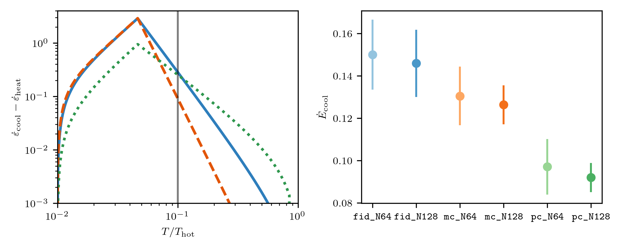
In order to test whether or not cooling at is truly indicative of cooling in the layer in the fully non-linear setting, we run a series of additional simulations with and but with modified cooling functions. These cooling functions are shown in the left panel of Figure 7. In particular, we compare the simulations with the fiducial cooling function (blue) with simulations which are identical except for (orange dashed), and and (green dotted). We refer to the first modification as mc as it modifies the mixed temperature () cooling time by a factor of 3, and the second modification as pc as it changes the peak temperature () cooling time by a factor of 3 but keeps the cooling time at unchanged.
The total cooling rates for simulations at resolution of are shown in the right panel of Figure 7. As we can see, large changes in the cooling at result in relatively small changes in the total cooling rate (comparing orange to blue points, they are consistent within errors) whereas a change to the peak cooling temperature that keeps the cooling at unchanged results in significant differences (comparing blue to green points). We conclude that is a more meaningful time-scale on which to measure the rate of cooling in the layer than .
References
- The theory of radiatively driven stellar winds. II. The line acceleration.. ApJ 259, pp. 282–301. External Links: Document Cited by: §I.
- Turbulent mixing layers in the interstellar and intracluster medium.. MNRAS 244, pp. 26P–29. Cited by: Appendix B, §I.
- Hydrodynamic and hydromagnetic stability. Cited by: Appendix B.
- The Anatomy of a Turbulent Radiative Mixing Layer: Insights from an Analytic Model with Turbulent Conduction and Viscosity. ApJ 950 (2), pp. 91. External Links: Document, 2211.01395 Cited by: §II.
- Marching Cubes 33: Construction of topologically correct isosurfaces. GRAPHICON’95. Cited by: §II.
- Fractal geometry of isoscalar surfaces in turbulence: Theory and experiments. Phys. Rev. Lett. 67 (13), pp. 1739–1742. External Links: Document Cited by: §I.
- The evaporation of spherical clouds in a hot gas. I. Classical and saturated mass loss rates.. ApJ 211, pp. 135–146. External Links: Document Cited by: §I.
- Der einfluss der turbulenz auf die flammengeschwindigkeit in gasgemischen. Zeitschrift für Elektrochemie und angewandte physikalische Chemie 46 (11), pp. 601–626. Cited by: §I.
- Magnetic fields in multiphase turbulence: impact on dynamics and structure. MNRAS 527 (1), pp. 991–1013. External Links: Document, 2307.06411 Cited by: Appendix A, §I.
- The regularity theory for the Mumford-Shah functional on the plane. arXiv e-prints, pp. arXiv:2308.14660. External Links: Document, 2308.14660 Cited by: footnote 10.
- Key Physical Processes in the Circumgalactic Medium. ARA&A 61, pp. 131–195. External Links: Document, 2301.10253 Cited by: §I.
- Geometric measure theory. Classics in Mathematics, Springer-Verlag. External Links: ISBN 9783540606567, Link Cited by: footnote 10.
- Thermal Instability.. ApJ 142, pp. 531. External Links: Document Cited by: §I, §IV.2.
- The Structure of Multiphase Galactic Winds. ApJ 924 (2), pp. 82. External Links: Document, 2108.05355 Cited by: §I.
- Multiphase Gas and the Fractal Nature of Radiative Turbulent Mixing Layers. ApJ 894 (2), pp. L24. External Links: Document, 2003.08390 Cited by: Appendix A, §I, §I, §I, §II, §IV.1, §IV.2, §IV.2.
- Turbulence: the legacy of a. n. kolmogorov. Cambridge University Press. Cited by: §III.2.
- The growth and entrainment of cold gas in a hot wind. MNRAS 480 (1), pp. L111–L115. External Links: Document, 1806.02728 Cited by: §I.
- Turbulent premixed flame propagation models for different combustion regimes. Symposium (International) on Combustion 23 (1), pp. 743–750. Note: Twenty-Third Symposium (International) on Combustion External Links: ISSN 0082-0784, Document, Link Cited by: §I, §I, §I, footnote 3.
- Array Programming with NumPy. arXiv e-prints, pp. arXiv:2006.10256. External Links: 2006.10256 Cited by: The Origin of Da Scaling: Suppressed Cooling in Fast-Cooling Mixing Layers.
- Matplotlib: A 2D Graphics Environment. Computing in Science and Engineering 9 (3), pp. 90–95. External Links: Document Cited by: The Origin of Da Scaling: Suppressed Cooling in Fast-Cooling Mixing Layers.
- Thermal instability and multiphase gas in the simulated interstellar medium with conduction, viscosity, and magnetic fields. MNRAS 505 (4), pp. 5238–5252. External Links: Document, 2012.05252 Cited by: §I.
- Superbubbles in the Multiphase ISM and the Loading of Galactic Winds. ApJ 834 (1), pp. 25. External Links: Document, 1610.03092 Cited by: §I.
- Instability of Evaporation Fronts in the Interstellar Medium. ApJ 779 (1), pp. 48. External Links: Document, 1310.2940 Cited by: Appendix B, §I.
- The Statistics of Supersonic Isothermal Turbulence. ApJ 665 (1), pp. 416–431. External Links: Document, 0704.3851 Cited by: footnote 7.
- Fundamentals of turbulent and multiphase combustion. John Wiley & Sons. Cited by: §I, §I.
- Geometry, Dissipation, Cooling, and the Dynamical Evolution of Wind-blown Bubbles. ApJ 970 (1), pp. 18. External Links: Document, 2405.02396 Cited by: §I.
- Efficiently Cooled Stellar Wind Bubbles in Turbulent Clouds. I. Fractal Theory and Application to Star-forming Clouds. ApJ 914 (2), pp. 89. External Links: Document, 2104.07691 Cited by: §IV.2.
- Efficiently Cooled Stellar Wind Bubbles in Turbulent Clouds. II. Validation of Theory with Hydrodynamic Simulations. ApJ 914 (2), pp. 90. External Links: Document, 2104.07722 Cited by: §I.
- Efficient implementation of marching cubes’ cases with topological guarantees. Journal of Graphics Tools 8 (2), pp. 1–15. External Links: Document, Link, https://doi.org/10.1080/10867651.2003.10487582 Cited by: §II.
- Marching cubes: a high resolution 3d surface construction algorithm. In Proceedings of the 14th Annual Conference on Computer Graphics and Interactive Techniques, SIGGRAPH ’87, New York, NY, USA, pp. 163–169. External Links: ISBN 0897912276, Link, Document Cited by: §II.
- Instability of supersonic cold streams feeding galaxies - IV. Survival of radiatively cooling streams. MNRAS 494 (2), pp. 2641–2663. External Links: Document, 1910.05344 Cited by: §I.
- The (Limited) Effect of Viscosity in Multiphase Turbulent Mixing. arXiv e-prints, pp. arXiv:2504.15345. External Links: Document, 2504.15345 Cited by: Appendix A, §I.
- Suppression of Shock X-Ray Emission in Novae from Turbulent Mixing with Cool Gas. ApJ 988 (2), pp. 211. External Links: Document, 2505.08907 Cited by: §IV.2.
- Tracing Multiphase Structure in the Circumgalactic Medium: Insights from Magnetohydrodynamic Turbulence Simulations. arXiv e-prints, pp. arXiv:2511.00229. External Links: Document, 2511.00229 Cited by: §I.
- Statistical fluid mechanics, volume ii: mechanics of turbulence. Dover Books on Physics, Dover Publications. External Links: ISBN 9780486318141, Link Cited by: §IV.2.
- Theoretical and numerical combustion. R.T. Edwards Inc.. External Links: ISBN 9781930217102, Link Cited by: §I.
- A Three-Dimensional Deflagration Model for Type Ia Supernovae Compared with Observations. ApJ 668 (2), pp. 1132–1139. External Links: Document, 0707.1024 Cited by: §I.
- Universal Structure of Turbulent Radiative Mixing Layers. arXiv e-prints, pp. arXiv:2509.03802. External Links: Document, 2509.03802 Cited by: §IV.1.
- AthenaK: A Performance-Portable Version of the Athena++ AMR Framework. arXiv e-prints, pp. arXiv:2409.16053. External Links: Document, 2409.16053 Cited by: §II.
- Radiative mixing layers: insights from turbulent combustion. MNRAS 502 (3), pp. 3179–3199. External Links: Document, 2008.12302 Cited by: Figure 6, Appendix A, Appendix A, Appendix A, Appendix A, §I, §I, §I, §I, §IV.1, §IV.1, §IV.2, footnote 6, footnote 8.
- A model for line absorption and emission from turbulent mixing layers. MNRAS 508 (1), pp. L37–L42. External Links: Document, 2105.11496 Cited by: §I.
- It’s Cloud’s Illusions I Recall: Mixing Drives the Acceleration of Clouds from Ram Pressure Stripped Galaxies. ApJ 911 (1), pp. 68. External Links: Document, 2102.05061 Cited by: §I.
- Scikit-image: image processing in python. PeerJ 2:e453, pp. 1–15. External Links: Document Cited by: §II.
- SciPy 1.0: fundamental algorithms for scientific computing in Python. Nature Methods 17, pp. 261–272. External Links: Document, 1907.10121 Cited by: The Origin of Da Scaling: Suppressed Cooling in Fast-Cooling Mixing Layers.
- The dynamic and gravitational instabilities of spherical shocks. ApJ 274, pp. 152–167. External Links: Document Cited by: Appendix B.
- Passive Scalars in Turbulent Flows. Annual Review of Fluid Mechanics 32, pp. 203–240. External Links: Document Cited by: §IV.2.
- On the local structure of a temperature field in a turbulent flow. Dokl. Akad. Nauk. SSSR 69, pp. 743–46. Cited by: §IV.2.
- Radiative turbulent mixing layers at high Mach numbers. MNRAS 520 (2), pp. 2148–2162. External Links: Document, 2205.15336 Cited by: footnote 2.
- The Phase Equilibrium and Dynamics of a Gas Volume That is Heated and Cooled. Soviet Journal of Experimental and Theoretical Physics 29, pp. 170. Cited by: §I, §I.
- A numerical model of premixed turbulent combustion of gases. Chem. Phys. Reports 14 (7), pp. 993–1025. Cited by: §I.