Convergence of an algorithm for constructing Lyapunov functions for switched systems using meshfree collocation
Abstract.
Switched systems are a class of dynamical systems where trajectories switch between different systems based on a switching rule. This rule can depend on time and/or the position of the trajectory in the state space. The existence of a Lyapunov function implies the existence of a uniformly asymptotically stable equilibrium point at the origin, which we prove in this paper. A method to construct Lyapunov functions for switched systems using meshfree collocation and quadratic programming was described in a related article. We prove that, under suitable assumptions, the algorithm described in this previous work converges as the fill distance between the collocation points tends to zero.
Key words and phrases:
Dynamical system, switched system, Lyapunov function, meshfree collocation, quadratic programming, convergence.2020 Mathematics Subject Classification:
Primary: 93D30, 93-08; Secondary: 34D20, 65L07, 90C20.1. Introduction
Lyapunov functions are a useful tool to show stability properties of a dynamical system and to determine the basin of attraction of equilibria. When a dynamical system is expressed as a system of differential equations, a (strict) Lyapunov function is a positive function that decreases along solutions of the system. For a smooth function this is equivalent to having a negative orbital derivative. The existence of a Lyapunov function implies that the system has an equilibrium point that is stable and attractive. The basin of attraction of the equilibrium point can be determined through sublevel sets of the Lyapunov function. For background, see [26], [17] and [19].
A construction method for Lyapunov functions for autonomous ODEs is developed in [13]. Meshfree collocation is used to find an approximation to the PDE , where represents the orbital derivative. To do this, finitely many collocation points are selected and the norm-minimal function such that the PDE is satisfied at these points is found. This method is extended in [9] where an approximate solution to a system of partial differential inequalities is found using quadratic programming. The approximate solution has been shown to converge to the solution of the system of partial differential inequalities as the fill distance decreases [10].
It is useful to construct Lyapunov functions for a variety of dynamical systems, including switched systems. Switched systems are a family of dynamical systems where a switching rule determines which system is “switched on”. This switching rule can depend on time and/or position in the state space. Switched systems where time-dependent switching takes place are called arbitrary switched systems, and systems where state-dependent switching occurs are called variable structure systems. These systems have widespread applications in science, engineering and economics, e.g. water quality control, manufacturing systems, or aircraft control. An overview of switched systems can be found in [20] and a review of results related to the stability of such systems can be found in [7].
Many methods have been developed to construct Lyapunov functions for switched systems. One such method is the algorithm developed in [14] to construct Continuous and Piecewise Affine (CPA) Lyapunov functions for arbitrary switched systems. This was then developed further to construct CPA Lyapunov functions for strongly asymptotically stable differential inclusions in [2] and [3], and control CPA Lyapunov functions for weakly asymptotically stable differential inclusions in [4]. The algorithm was advanced in [15] and [16] and applied to variable structure examples. A different algorithm has been developed to construct Lyapunov functions for switched systems in [21] using meshfree collocation and quadratic programming. A usual assumption in the literature is that the switched system follows one switching rule; however, the switched system defined in [21] allows switching based on time and/or position in the state space. To construct a Lyapunov function for this system, an approximate solution to a system of partial differential inequalities is found, where indicates the system that is “switched on”, is the orbital derivative with respect to and is a non-positive function which is zero at the equilibrium. In this paper, we show that under suitable assumptions the approximate solution converges to a solution of the system of partial differential inequalities.
Overview of the paper:
This paper provides the theoretical backbone of the algorithm to construct a Lyapunov function for a switched system that appears in [21]. We show that this algorithm converges as the fill distance decreases if there exists a Lyapunov function for the system. Section 2 defines this switched system which allows for time- and state-dependent switching and a corresponding Lyapunov function, and introduces sufficient conditions for the equilibrium point of the system to be uniformly asymptotically stable. In Section 3 we examine a system of partial differential inequalities, the solution of which is a Lyapunov function for the switched system, and discretise it to find a minimisation problem (3.10). The solution to this minimisation problem is shown to converge under certain assumptions when the fill distance (3.13) decreases (i.e. the discretisation gets finer) in Section 3.3. In Section 4, we show equivalence of (3.10) to the minimisation problem from [21] which means the convergence theorem from Section 3.3 applies to the algorithm in [21]. This section also contains details of the method described in [21] to construct a Lyapunov function for a switched system; this is summarised in Algorithm 1. Finally, Section 5 gives examples where Algorithm 1 is applied to two systems. In the following table we give our main results with brief descriptions and where they can be located.
| Section 2.2, Theorem 2.7: |
| Existence of a Lyapunov function for the switched system implies uniform asymptotic stability of its equilibrium point. |
| Section 3.3, Theorem 3.5: |
| The solution to the minimisation problem (3.10) converges to a Lyapunov function for the switched system as the fill distance decreases if a Lyapunov function for the system exists. |
| Section 3.4, Corollary 3.10: |
| A way to choose the collocation points is given that is a sufficient condition for the fill distance assumption from Theorem 3.5 to be satisfied. |
| Section 4.2, Lemma 4.2: |
| The minimisation problem (3.10) is equivalent to the minimisation problem (8) from [21] and thus the algorithm from [21] converges. |
Acknowledgements
Jay Ward acknowledges support by the EPSRC, via a PhD studentship funding 2889464. Nicos Georgiou and Peter Giesl gratefully acknowledge partial support from the Dr Perry James (Jim) Browne Research Centre at the Department of Mathematics, University of Sussex.
2. Switched systems
In this paper, we consider switched systems that allow arbitrary switching, variable structure switching, or a combination of the two. We define a corresponding Lyapunov function and state the conditions needed for uniform asymptotic stability of the equilibrium point. The switched system we are considering is defined in (2.1) in the same way as in [21]. Systems are defined on subsets of the state space, with the union of these subsets making up the whole state space. The subsets may overlap; wherever this occurs, the system may switch arbitrarily to a different trajectory. This set-up was discussed in [20], and it was stated that this switched system will have an asymptotically stable equilibrium point if there exists a Lyapunov function for each system in the region where it is defined. This allows multiple Lyapunov functions to be considered, as done in [5] and [18]. On the other hand, [21] states a theorem that the existence of a single Lyapunov function for a switched system implies that it has an asymptotically stable equilibrium point. We prove a stronger statement within this section: the existence of a Lyapunov function implies uniform asymptotic stability of the equilibrium point.
In Section 2.1 we define a switched system and a Lyapunov function for the system. We also list the assumptions we have on this system in Assumptions 2.2. In the following Section 2.2, we define what is means for this switched system to have a uniformly asymptotically stable equilibrium point, and show that a sufficient condition for uniform asymptotic stability is the existence of a Lyapunov function. This result is given in Theorem 2.7.
2.1. Problem formulation
Let be a bounded domain with Lipschitz boundary and define a switched system by autonomous systems of differential equations
| (2.1) |
where for in the maximal interval of existence. For each we assume that is the restriction to of a vector field defined on an open neighbourhood of where , and is finite. Assume that , and that the sets are closed for all . We also assume that for the values where the functions have an equilibrium point at the origin, i.e. . The sets are also a covering of , i.e.
| (2.2) |
Remark 2.1.
We assume that for in the maximal interval of existence since we are mainly interested in the basin of attraction (see Definition 2.5) of the equilibrium point at the origin. Solutions starting in the basin of attraction will be defined for all positive times.
The index in (2.1) can change depending on time and/or position in the state space. The sets enable us to examine systems where time- and state-dependent switching can occur. Within the intersections of these sets the system switches arbitrarily between the functions that are defined. If the boundary of one of these intersections is reached, a state-dependent switch must take place if the function that is currently “switched on” is undefined in the new subset.
To illustrate this, consider the switched system
| (2.3) |
and a potential partition of the domain as given in Figure 1. In the set both functions and are defined and the system may switch arbitrarily between them. Suppose the trajectory reaches the left boundary and moves into the subset . If the index is it will change to ; if the index is already it will stay the same.
We indicate how changes in the system (2.1) using the following (anchored) switching sequence indexed by an initial state
| (2.4) |
This switching sequence completely describes a trajectory of the system (2.1) according to the following rule: means that the system evolves according to for . This can be used to describe a switched system that allows for both time- and state-dependent switching, as some of these times can correspond to the time at which a state change that causes the system to switch takes place. For we define
| (2.5) |
to be a shift operator, where is the switching sequence after time has passed. Set to be the set of all switching sequences that can occur when starting from the initial state . A possible system trajectory is denoted by for . We can define for to be the interval upon which only one system is “switched on”. We assume that in any finite interval with that is finite, i.e. there is a finite selection of indices that are “switched on” in the interval , see (7) from Assumptions 2.2.
We now list the assumptions that we have made in the set-up of our switched system.
Assumptions 2.2.
-
(1)
For each we assume that is the restriction to of a vector field defined on an open neighbourhood of where .
-
(2)
and the sets are closed for all .
-
(3)
The sets for all are a covering of .
-
(4)
If then .
-
(5)
is a bounded domain with Lipschitz boundary with .
-
(6)
is finite.
-
(7)
Switching sequences are chosen so that only finitely many switches occur in finite time.
A Lyapunov function of the switched system (2.1) is a function that is non-increasing along the solutions of each differential equation in the system. For our purposes we say that , is a Lyapunov function for the system (2.1) if and only if
| (2.6) |
holds for all and all such that , where for all . The function decreases along solutions of each differential equation in the system and is zero at zero, meaning that this is actually a strict Lyapunov function for the system (2.1).
The function from (2.6) will not just be decreasing along the solutions of each differential equation in the system (2.1), it will also be decreasing along solution trajectories of the system as a whole. To show this, we use the switching sequence defined in (2.4) to describe the solution trajectories of the system (2.1).
Lemma 2.3.
Proof.
Choose , and assume that . Recall that for are intervals upon which only one system from (2.1) is “switched on”, where and are switching times (see (2.4)). We wish to show that in both cases where and , we have .
First, we show this for . If we integrate (2.6) on the interval we have
| (2.7) |
where the first equality uses that . The integral of the right-hand-side of (2.6) is always negative (except at ) due to being positive. Consequently, the difference found in (2.7) is negative and .
Now we use this to show that if , then the inequality still holds. Integrating (2.6) on the interval is done in the same way as (2.7), and we find that . As we have that is not in the interval we can assume that it is a member of a different interval where , . This means that
| (2.8) |
where we have using (2.7) and that . This gives us that . Therefore, due to the properties of as described in (2.6), it strictly decreases along solution trajectories of the system (2.1). ∎
In the following section we find the sufficient conditions for the uniform asymptotic stability of the equilibrium point of the system (2.1).
2.2. Asymptotic stability
In this section, we prove that the existence of a Lyapunov function of the form (2.6) for all ensures that the equilibrium point at the origin of system (2.1) is uniformly asymptotically stable. This is a new variation on previous results for switched systems as two switching rules can be incorporated and the asymptotic stability is uniform. We prove this by adapting classical Lyapunov methods in Theorem 2.7; however, before this we introduce Lemma 2.6 which is necessary to complete this proof.
The -flow is a continuous mapping with , and which maps the state of the system (2.1) at time to the state at time dependent on the switching sequence , i.e. . The flow for sets is the set of all points which are reached after a time from any starting point under the -flow for all . This can be written as
| (2.9) |
The -flow has the properties that and , where is the shift operator defined in (2.5). Using this property we can also show that . Now, using this notation, we introduce the definition of a positively invariant set.
Definition 2.4.
(Positively invariant set) Let . We say is positively invariant if for all .
We can now define the uniform asymptotic stability of the equilibrium point for the system (2.1).
Definition 2.5.
(Uniform asymptotic stability and basin of attraction) The equilibrium point of system (2.1) is stable if for all there exists a such that for all the solution exists and
| (2.10) |
The equilibrium point of system (2.1) is uniformly asymptotically stable if it is stable and there exists a such that for all there exists a such that for all times , we have that
| (2.11) |
The set
| (2.12) |
is called the basin of attraction of , where is a uniformly asymptotically stable equilibrium point.
Lemma 2.6.
Let be the equilibrium point of the system (2.1). The following two statements are equivalent:
-
(i)
is stable.
-
(ii)
For all neighbourhoods of there is a neighbourhood of which is positively invariant.
Proof.
We can write the stability property (2.10) in a way that is more relevant for this proof. Define
| (2.13) |
to be an -neighbourhood of the origin. Then is stable if and only if for every neighbourhood there exists a neighbourhood with such that for all .
(i)(ii): As we are assuming that is stable, the property described below (2.13) holds true. Let be a neighbourhood of and be small enough such that . Define . The set is a neighbourhood of as . Then, using that , we have
So there is a neighbourhood of that is positively invariant.
(ii)(i): We now assume that property (ii) holds and wish to show that is stable. As for all neighbourhoods we can find a that is positively invariant, for any there must exist a positively invariant subset that is also a neighbourhood of . Since is a neighbourhood of , there exists such that . Since is positively invariant,
Therefore, we have shown that for every neighbourhood of there exists a neighbourhood of such that for all . This tells us that the equilibrium point is stable. ∎
We can now prove the following main result which shows that the existence of a Lyapunov function implies that the equilibrium point of the system (2.1) is uniformly asymptotically stable.
Theorem 2.7.
Proof.
This proof is separated into two parts: first stability, and then uniform asymptotic stability. In the process of doing this we show that if satisfies (2.14) and is compact then it is a subset of the basin of attraction of , we briefly describe how this has been done at the end of the proof.
We can find an such that (defined in (2.13)) satisfies . Fix and let
| (2.15) |
Since is a continuous function with if and only if , there is a (with ) such that for all .
Now for to be stable we want to show that implies for all and all . Assume that this is false. Then there is an , a time and a such that is in up to the time , when it lies on the boundary, i.e. for all , . Since (2.6) implies that is decreasing along solution trajectories as was shown in Lemma 2.3, implies that . This contradicts (2.15) since .
Now that we have shown stability of the equilibrium point , we wish to show that it is also uniformly asymptotically stable. We do this by way of contradiction. We assume the opposite of (2.11) which means that
-
(1)
for all neighbourhoods of there exists a neighbourhood of where for all there exists a time , and a with .
Here we have assumed that as the proof of the alternative is trivial due to the stability of . As we know that there exists a Lyapunov function that satisfies properties (2.6), we know that this is positive except at the origin (and decreases along solution trajectories). Therefore, we can find a level set (2.14) that is a compact subset of . Now we choose such that . By assumption (1) there exists an with . Using Lemma 2.6 we find a positively invariant neighbourhood of which we label , where . Now by the properties of we know there exists a level set with such that . Finally, define the set . The set-up of these sets is illustrated in Figure 2.
Since is compact and is a neighbourhood of the origin, the set is compact and does not contain the origin. For each such that , the function is continuous and strictly positive on the compact set . Hence
Since is finite, we may define
Then, for all and ,
| (2.16) |
This means that for all we have that . Choose the time . Now we have fixed our , and that we use in (1) and it now becomes
-
()
there exists a , and a such that .
To obtain a contradiction we consider two separate cases which cover all of the elements of . The first case we look at is , and the second case is .
Case 1: . As is a positively invariant set we have that for all and . This gives us a contradiction to () for any .
Case 2: . To find a contradiction to () we prove the following lemma and use the arguments made in Case 1.
Lemma 2.8.
Proof.
We prove this by way of contradiction. Assume that there exists an and a switching sequence such that for all . Then . As then , which means that for all and , as is decreasing. Then, using our assumption we have for all . Using the definition of ,
| (2.17) |
Integrating (2.6) with techniques similar to (2.7) between and and using (2.16) we find that for all , and for
This gives us a contradiction to (2.17). Therefore, we have shown this lemma to be true. ∎
As the combination of Case 1 and 2 contradicts assumption (). This means we have a contradiction to assumption (1) and is uniformly asymptotically stable.
In the process of showing is uniformly asymptotically stable, we have shown for all there exists a such that for all , and we have . This is a stronger statement than is needed and therefore is enough to prove that the compact level set (2.14) is a subset of the basin of attraction of , defined in (2.12). ∎
3. Minimisation problem
We wish to find a minimisation problem where the solution is an approximation of a function that satisfies the conditions in (2.6). This allows us to construct a Lyapunov function for the switched system (2.1). A similar method is used in [9] for autonomous ODEs. There, the authors construct a Lyapunov function for a single system by finding a solution to the system of partial differential inequalities where denotes the orbital derivative, and is negative. To generalise this method, we define for all the linear differential operator
| (3.1) |
where for each we assume that is the restriction to of a vector field defined on an open neighbourhood of where . We wish to solve
| (3.2) |
where are continuous functions on that are negative for all , . Finding a solution to this system of partial differential inequalities is equivalent to finding a Lyapunov function as in (2.6).
In Section 3.1 we define a reproducing kernel Hilbert space . We choose an approximating function of the function (3.2) to belong to such a space. We also introduce some properties of that are used later in Section 3.3 and in Algorithm 1. In Section 3.2 we discretise problem (3.2) by selecting collocation points. This gives us a minimisation problem which we solve to find an approximating function . In Section 3.3 we show that as the fill distance (3.13) decreases the approximating function converges strongly to . This result is contained in Theorem 3.5. An assumption on the fill distance in this theorem is addressed in Section 3.4, where we present a way of choosing the collocation points under which the assumption holds.
3.1. Reproducing kernel Hilbert spaces
The solution to the minimisation problem (3.10), see Section 3.2, belongs to a reproducing kernel Hilbert space . We recall various properties of these spaces within this section, as well as specifying the reproducing kernel we will be using in the construction of the function in Section 4.4. For more information on reproducing kernel Hilbert spaces, see [24].
Definition 3.1.
(Reproducing Kernel Hilbert Space (RKHS)) Let . A Hilbert space of continuous functions with inner product is called a reproducing kernel Hilbert space, abbreviated RKHS, if there is a function with
-
(1)
for all
-
(2)
for all and all .
The function is called the reproducing kernel of . The reproducing kernel is called positive definite if for any pair of pairwise distinct points the matrix is positive definite.
As in [10], the reproducing kernel Hilbert spaces that we consider are Sobolev spaces . We use the definition of the Sobolev space found in [25] and set so that for
| (3.3) |
with scalar product . If is not an integer, then we use operator interpolation theory to define the space and norm, for more details see [1] and [6].
The following two lemmas will be used multiple times in Section 3.3, in the proof of both Theorem 3.5 and Lemma 3.6.
Lemma 3.2.
If is a bounded domain with Lipschitz boundary, then the space for is a RKHS.
Proof.
If is a bounded domain with Lipschitz boundary, then there exists a continuous linear extension operator [24] . This has the properties and for all with a fixed constant . As stated in [10], a consequence of the existence of the extension operator is the Sobolev embedding theorem for , which tells us that if . As this is a continuous embedding, we have that for some . The first norm can be rewritten as follows , which tells us that
This shows continuity of the point evaluations , so our space is a RKHS [24]. ∎
The explicit form of the reproducing kernel of is usually unknown. To find a suitable substitute we use the following Lemma 3.3 which can be found in [10] and was developed with results from [24]. The method of finding a suitable reproducing kernel for can be summarised as follows: choose a reproducing kernel that delivers an equivalent norm to the standard norm on , and restrict it to find a reproducing kernel for . A reproducing kernel that delivers this equivalent norm can be chosen to be a translation-invariant function with certain properties on its Fourier transform. can be chosen to be radial and, in particular, a Wendland function (see [10]), which we discuss further in (3.4).
Lemma 3.3.
Assume has a Fourier transform satisfying
where are constants, and . Let be a bounded domain with a Lipschitz boundary. Let be defined by , . Then there exists an inner product on such that is the reproducing kernel of with respect to this inner product. The norm induced by this inner product is equivalent to the standard norm on , i.e. there are constants such that
Proof.
In the construction of the function we are using meshfree collocation. This method has been applied to the construction of Lyapunov functions for autonomous ODEs in [13] and [9]. Following the methods explained here we assume that the reproducing kernel of the Hilbert space is given by a radial basis function through .
For this radial basis function we use Wendland functions, which are a family of functions introduced in [22] and [23]. Wendland functions are positive definite with compact support, and are polynomials on their support. We define , where is a Wendland function with , a smoothness parameter and . The reproducing kernel Hilbert space that corresponds to this Wendland function is norm-equivalent to the Sobolev space . Wendland functions are defined by recursion: for ,
| (3.4) |
for , where if and otherwise.
Using recursion, define for and . Note that exists if the smoothness parameter of the Wendland functions is sufficiently large.
3.2. Discretised problem
We now discretise our problem. Fix collocation points
| (3.5) |
where is the total number of collocation points, and take subsets of these points
| (3.6) |
for , where is the number of collocation points in the subset . We have that for all , and
The sets are not necessarily distinct as the sets can overlap.
We can now define
| (3.7) |
and seek to find a function that satisfies
| (3.8) |
for .
Another way to express (3.8) would be to find a function using the information generated by the functionals , i.e. for all and . We define these functionals as the orbital derivative with respect to (3.1) applied at a particular collocation point , i.e.
| (3.9) |
for all and , with being Dirac’s delta distribution.
The optimal reconstruction of is then given by the solution of the problem
| (3.10) |
We now state the following lemma which is similar to one in [9], which shows that this minimisation problem has at most one solution.
Lemma 3.4.
The problem (3.10) has at most one solution.
Proof.
Assume is a minimiser and is a solution of
| (3.11) |
Then . We assume in contradiction to this that . For , satisfies (3.11) and
for a suitable choice of . This is a contradiction to being a minimiser.
Now let be minimisers. This implies that both and are greater than or equal to zero, giving
which shows ∎
3.3. Convergence
In this section we show that as the fill distance (3.13) decreases, the solution converges strongly to the solution of the original system of partial differential inequalities (3.2). We do this by adapting a theorem from [10] for autonomous ODEs.
Theorem 3.5.
Let be a bounded domain with Lipschitz boundary. Let for be such that (2.1) is the restriction to of a vector field defined on an open neighbourhood of where . Let be linear differential operators as defined in (3.1). Let be continuous functions and let (3.3) with norm given by an appropriate reproducing kernel. Consider the optimisation problem for
| (3.12) |
and the sequence of optimisation problems:
For we choose points . For the sets are defined as , i.e. are elements of for . We also assume that for fixed the fill distance
| (3.13) |
Furthermore, assume that there exists a that satisfies the constraints of (3.12). For each fixed let satisfy the constraints of the minimisation problem for
| (3.14) |
with for some where
| (3.15) |
Then the optimisation problem (3.12) has a unique solution and the functions converge strongly in to as .
Before we prove this theorem we prove a lemma that shows how the minimisation problem (3.14) is related to our original problem (3.10).
Proof.
We first start by seeing that as and because of having a Lipschitz boundary, is indeed a RKHS, as we have seen in Lemma 3.2. Now we can use Lemma 3.3 and choose an inner product on and a reproducing kernel given by a positive definite function as , . The norm induced by this inner product is equivalent to the standard norm on , and we use this inner product and induced norm as the inner product and norm on , denoting . As maps continuously to and as implies by the Sobolev embedding theorem [1], the functionals belong to as they are bounded linear operators. Hence, for a fixed , problem (3.14) is indeed (3.10) with these , , and where . ∎
Now we provide the proof of the convergence theorem.
Proof of Theorem 3.5.
Fix . We show in the following steps that the sequence of solutions of (3.14) converges strongly to an element which is the unique solution of (3.12). Due to the result of Lemma 3.6, this implies that if the fill distance (3.13) decreases, the solution of the minimisation problem (3.10) converges strongly to a solution of the system of partial differential inequalities (3.2).
The proof is structured as follows: in Step 1 we show that a subsequence of weakly converges to a function , in Step 2 we show that satisfies the constraints of (3.12), in Step 3 using both previous steps we can now show that the subsequence strongly converges to , and finally in Step 4 we show that is a unique minimiser. We then finish the proof by showing that our original sequence must converge strongly to . We use the notation and .
Step 1: We have a that satisfies the constraints of (3.12), which means that
This means that
Thus satisfies the constraints of (3.14), which means by assuming that there is a feasible solution to (3.12) we also have the assumption that there is a feasible solution to (3.14) for each . Therefore, using the definition of in (3.15), there exists that satisfies the constraints of (3.14) with .
Hence we have
| (3.16) |
In particular,
| (3.17) |
thus is bounded for all . As bounded sets in Hilbert spaces are relatively compact in the weak topology, there is a subsequence of which we also denote by , that weakly converges to a function . From
it follows using (3.16) that
| (3.18) |
Step 2: Now we use the kernel representation to show that for all and , where is the weak limit of the subsequence , i.e. that satisfies the constraints of (3.12).
We can define where is the Riesz representative of . This gives that
| (3.19) |
as converges weakly to .
Next we can see from Lemma 3.2 that as and has Lipschitz boundary, is also a RKHS. We can again use Lemma 3.3 to give us a reproducing kernel where . Since we can also use the Sobolev embedding theorem [1] to give which implies there exists an such that
| (3.20) |
for all . Indeed, using that , the Sobolev embedding theorem gives us the inequality . We then find that
which gives us the original inequality for all .
Now we can take and a on the line between and such that, using that is a bounded operator with constant ,
| (3.21) | |||||
for all where . The second equality is deduced using , the properties of inner products and the properties of as a reproducing kernel as described in Definition 3.1.
We have set out to show that for all and , which is the same as showing that for all we have .
We fix . By (3.19) we know that there exists such that for all
| (3.22) |
Since is continuous at there exists a such that for all with
| (3.23) |
We also know by (3.13) that there exists such that for all there exists a with
| (3.24) |
Therefore, for and using the statements (3.22), (3.21), (3.24) and (3.23) as well as we have that
Step 3: Due to our findings in Step 2 that satisfies the constraints of the continuous problem (3.12), it satisfies them in particular at every collocation point . Thus is feasible for the discretised problem (3.14), for every . Therefore, we have and thus
| (3.25) |
for all . This implies that holds. Now using (3.18) it follows that
and as
it follows that converges strongly to .
Step 4: It remains to show that is a unique minimiser. Firstly we show that is a minimiser. To do this we take a that satisfies the constraints of (3.12), which implies that for every , also satisfies the constraints of (3.14). Therefore we have that and, if we take , we have that due to the strong convergence, so . This shows is a minimiser.
To show it is a unique minimiser we assume is a minimiser and satisfies the constraints of (3.12) and show that
| (3.26) |
Indeed we assume . If we let we can see for (which satisfies the constraints) we have
for a suitable choice of . This contradicts being a minimiser.
Two assumptions are made for this convergence result to hold. One assumption is on the fill distance of the collocation points converging to zero, and sufficient conditions for this to hold are given in the following section. The other assumption is that there exists a function that satisfies the constraints of the minimisation problem (3.12). A sufficient condition for this is the existence of a Lyapunov function for the switched system (2.1). We will explore sufficient conditions for the existence of a Lyapunov function for this system in future work.
3.4. Fill distance assumption
In this section, we consider the assumption made in (3.13) that states that the fill distance tends to zero as the number of collocation points tends to infinity. One way of choosing the collocation points is setting with . Then for all we have a subset of the collocation points . If we know that the sets have Lipschitz boundary and we choose the collocation points in this way, the fill distance converges as we want for Theorem 3.5.
Any set that is bounded with Lipschitz boundary satisfies an interior cone condition, see Section 4.7 on page 67 of [1]. For every point of a set satisfying an interior cone condition there is a direction (given by unit vector ) such that a cone with angle and radius is contained within . This has been illustrated in Figure 3, and a formal definition is given below, see [24].
Definition 3.7.
(Interior Cone Condition) A set is said to satisfy an interior cone condition if there exists an angle and a radius such that for every a unit vector exists such that the cone
| (3.27) |
is contained in .
See the following lemma, also from [24], showing that there is a ball contained within this cone.
Lemma 3.8.
Suppose that is a cone defined as in (3.27). Then for every the closed ball with centre and radius is contained in . In particular, if is a point in this ball, then the whole line segment , , is contained in the cone.
We now prove the following lemma that we go on to use in the proof of Corollary 3.10. There we detail sufficient conditions for the assumption (3.13) to hold.
Lemma 3.9.
Set the collocation points to be and take subsets . Fix and assume satisfies an interior cone condition. Then for all there exists such that for all and there exists a collocation point such that .
Proof.
Fix . The set satisfies an interior cone condition, as described in Definition 3.7. For a point its respective cone is denoted . Applying Lemma 3.8 we see that for every the closed ball with centre and radius is contained within the cone . An example of a cone and a ball for a point is shown in Figure 4.
Throughout this proof we use the following two choices of variables. Choose to be such that
| (3.28) |
and choose to be
| (3.29) |
We prove this lemma in two steps. Firstly we show that for there exists a collocation point within the ball . Then, using the restriction placed on in (3.28), we show that the distance between this collocation point and an arbitrary point is bounded by .
Step 1: For and all there will exist a collocation point within the ball if
| (3.30) |
This is because the distance collocation points are from each other is , and the smallest distance between the collocation points such that there could be no points within a ball is . We show this to be the case in the following way: for this is clear as the distance between the collocation points is the same as the diameter of the ball. For we can show this using contradiction. Assume that the distance between the collocation points is with and there are no collocation points within the ball. Let be a collocation point that is closest to the point . The distance between and must be less than or equal to half of the distance between the collocation points multiplied by , as a unit hypercube’s longest diagonal in dimensions is equal to . This implies that
which is a contradiction. In Figure 5 we show the point with a ball of radius around it. It can be seen here that the smallest distance that is between the collocation points such that there are no points within the ball is .
In the choice of as given in (3.29) there are two cases, one is when the distance is greater than one, and the other is when it is between zero and one. We consider both cases and in both show that when the inequality (3.30) holds.
Case 1: is greater than one. The collocation points are chosen to be with . The distance collocation points are from each other is . Therefore, when is greater than one (3.30) holds.
Therefore, when where is defined in (3.29), there exists a collocation point in the ball .
Now we can use this lemma to see that choosing the collocation points as in Theorem 3.5 is a sufficient condition to satisfy the assumption on the fill distance.
Corollary 3.10.
Choose with , where are elements of for . Assume the sets satisfy an interior cone condition. Then the fill distance defined in (3.13) satisfies
Proof.
The result of Lemma 3.9 implies that for any there exists an such that for all and there exists a collocation point such that
∎
4. Construction using quadratic programming
In this section we show that the minimisation problem (3.10) defined in Section 3.2 is equivalent to the minimisation problem (4.12), which appears as equation (8) in [21]. Hence, we can apply Theorem 3.5 and see that the minimisation problem (4.12) converges as the fill distance decreases. We state techniques employed previously in [21] to find a solution to (4.12). This solution is a Lyapunov function for the system (2.1).
The techniques to find a solution to (3.10) are summarised in the following algorithm that can also be found in [21]; this algorithm is implemented using MATLAB code for the examples in Section 5.
Section 4.2 provides details on the collocation points and how these relate to the collocation points given in Section 3.2. This section also contains Lemma 4.2, where we show that the minimisation problems (3.10) and (4.12) are equivalent. The methods contained within [21] to find a solution to the minimisation problem (4.12) are explained briefly in Sections 4.3 and 4.4. With regard to Algorithm 1, details on steps and can be found in Section 4.3, and on steps , and in Section 4.4.
4.1. Partitioning the state space
We define the following sets from [21] for ,
| (4.1) |
Figure 6 illustrates a partition for the switched system (2.3), visualised previously in Figure 1. Here and the sets corresponding to , and are nonempty and partition the state space. These are defined as , and .
Lemma 4.1.
Proof.
First we show (4.2), which we do by showing that
| (4.3) |
The first statement is immediate due to the definition of in (4.1). To show the second statement we take . Due to (2.2), we know that must be contained in at least one of the sets for , and we denote as the nonempty subset of that contains exactly all of the ’s such that is in . This means that for , . Therefore, by the definition in (4.1), so we have that
| (4.4) |
showing the second statement from (4.3). This tells us that (4.2) holds.
To prove the second part of the lemma we assume without loss of generality that there exists a that is in both and for . As and are distinct, there must be an element that is in exactly one of or . Consequently, and ; however, this is not possible, so there is no that is in both and which implies . ∎
For our algorithm we refer to the total number of subsets that induce a nonempty as , i.e. in the case of Figure 6 we would have . This number is bounded above by as there are elements in the set and we cannot have . This enables us to label these subsets as where and we can write the elements of each of these sets as , with where . In Figure 6 we have labelled with , with and and with .
4.2. Equivalent minimisation problem
Using this set-up we now show that the minimisation problem (3.10) is equivalent to the minimisation problem (8) from [21]. The minimisation problem (3.10) has constraints that need to be satisfied for each collocation point for all and . On the other hand, in the minimisation problem from [21] the constraints are imposed at each collocation point in each set for . Therefore, we need to fix collocation points in the sets and show how these are related to the collocation points in the sets . We define the collocation points in the set to be
| (4.5) |
where is the set of collocation points in (3.5). Here is the number of collocation points in .
In Figure 7 we show how the collocation points (3.5), (3.6) for and for are related using the example discussed before in Figures 1 and 6.
We can now express some properties of the collocation points , and . In the same way as the sets , the union of the sets for is the whole set of collocation points . This is written as
We can also state that if is an element of the sets for , and no other sets for , i.e.
we have that
| (4.6) |
We can see this in the example shown in Figure 7. The set is the union of the sets and , and here the set of collocation points for the set is the union of the collocation points and , which are the collocation points for the sets and , respectively. Also, the number of collocation points for the set is equal to the sum of the number of collocation points for the sets and , i.e. . Finally, the sets of collocation points are distinct as the sets are distinct, which means
where is the total number of collocation points (3.5).
These collocation points have been taken in the same way as in [21], which means we can use the techniques from this article to find a minimisation problem. This is the same method as used in Section 3.2. Define for all and the linear differential operator
| (4.7) |
where for each we assume that is the restriction to of a vector field defined on an open neighbourhood of for and . The system of partial differential inequalities we wish to solve is
| (4.8) |
where are continuous functions that are negative for all , .
Discretising using the collocation points (4.5) and the values
| (4.9) |
gives us
| (4.10) |
for , where is the approximating function we wish to find.
As shown in [21], (4.10) can also be expressed using functionals. We look to find a function using the information generated by the functionals , i.e. for all , and . We define these functionals as the orbital derivative (4.7) applied at a particular collocation point , i.e.
| (4.11) |
for all , and . We have introduced this definition of the functionals here so it is more easily comparable with that in Section 3.2, however the elements of the set are reordered for each collocation point in the following section when we select a basis of the functions at this point, see (4.16).
As in [21], the optimal reconstruction of is given by the solution of the problem
| (4.12) |
We show that this problem is equivalent to the previous one found in Section 3.2 in the following lemma.
Proof.
Another way of writing the constraints of (3.10) using the definition of the functionals (3.9) is
| (4.13) |
for all and . Similarly, another way of writing the constraints of (4.12) using the definition (4.11) is
| (4.14) |
for all , and .
In the first part of this proof we show that satisfying the constraints (4.14) means that the constraints of (4.13) are satisfied, and in the second part we show the reverse.
(4.14) (4.13): Fix and . This gives us a specific collocation point . Let be the sets such that is an element for , and no other set for . This means that (4.6) holds and we have that
Therefore, there exists a for some and a such that . As we have that , there exists a such that . Now using this and in (4.14) we have proven this implication.
4.3. Selection of basis
If the functionals are linearly independent, we can use techniques from [24] to find a solution to the minimisation problem (4.12). However, this is not necessarily the case and we must use techniques previously described in [21] to deal with this. We fix a point , consider whether for are linearly independent, and if not, select a basis of the space spanned by these vectors.
To this end, fix and define the set
| (4.15) |
to be a set of indices such that the vectors with are a basis of
with being its rank. The elements of are labelled where . We allow the case where the vectors are all linearly independent, this would mean .
Therefore, we consider the vector
| (4.16) |
and write its components as for . This means we fix an ordering of the set for the collocation point where the indices that represent the basis are at the beginning of the vector. We find the vector (4.16) for each point for and .
From this point onward when we refer to the functionals we mean the definition (4.11) but replacing with the components from the vector (4.16).
For notational convenience we now define
| (4.17) |
From (4.16) we have that the functionals for are a basis for the whole set of functionals with . Therefore, the functionals at the point are expressed as a linear combination of this basis and we write this as
| (4.18) |
for all , for some appropriate . We assemble the coefficients for all of the collocation points as elements of a matrix such that
| (4.19) |
where is the identity matrix accounting for the coefficients for , , and is a block diagonal matrix that contains the remaining coefficients. The structure of this matrix is described in [21].
4.4. Quadratic programming problem
We now wish to show that the solution of (4.12) with the functionals defined above is of the form
| (4.20) |
where the coefficients are elements of the vector which satisfies
| (4.21) |
To find the matrices and we applied our functionals to our proposed solution (4.20) and used the inequalities in (4.12).
The elements of are
| (4.22) |
for , , , and . This matrix is symmetric and accounts for the linearly independent functionals. Applying the matrix (4.19) accounts for the linearly dependent functionals as a linear combination of the independent ones (4.18). The values of the vector are the elements from the minimisation problem (4.12) for all , and .
We can also see that minimising as in (4.21) is the same as minimising in the following way
Now we are able to show that if there is a feasible solution to (4.21), the solution of (4.12) is of the form (4.20). We do this with the following lemma and theorem, the proofs of which are found in [21].
Lemma 4.3.
Theorem 4.4.
Remark 4.5.
We can check if there is a feasible solution to (4.21) computationally; then there exists a unique minimiser to each discretised problem (3.14). This is due to Theorem 4.4 as we know that there will exist a Lyapunov function for the system of the form (4.20). We choose these functions as our sequence in Theorem 3.5 with .
5. Examples
In this section we give two examples where we construct Lyapunov functions for switched systems using Algorithm 1. Example 5.1 is a non-linear arbitrary switched system and Example 5.2 uses a combination of arbitrary and variable structure switching in . In both of these examples we have taken the Lyapunov function that is constructed by our algorithm, and computed a new Lyapunov function . This function has its minimum value at zero ensuring we meet the assumption outlined in (2.6). We are able to do this as the orbital derivatives of and are the same.
The Wendland function that we use in the implementation of Algorithm 1 is from [8] which means that we have
| (5.1) |
where .
Example 5.1.
(Non-linear arbitrary switched system) and the values of the vector are found using that for all and . Consider the following autonomous systems with asymptotically stable equilibrium points at the origin
| (5.2) |
and
| (5.3) |
The system (5.2) is from Exercise 2.4 in [19], and (5.3) is from Example 1 in [11]. In this example we switch arbitrarily between these two systems over the whole space . This is written as
| (5.4) |
where . We apply our algorithm using and , where . The collocation points are selected to be , this gives us 48 collocation points in total. The Lyapunov function produced for this system can be seen in Figure 8, and its orbital derivatives in Figure 9 which are negative except at the origin.


Example 5.2.
(Non-linear arbitrary and variable structure system in ) and the values of the vector are found using that for all and . Take the following two systems with asymptotically stable equilibrium points at the origin
| (5.5) |
and
| (5.6) |
The system (5.5) is from Example 2 of [11], and (5.6) is from Exercise 4.32 of [19]. We define on the whole space , and on a subset of defined as
| (5.7) |
The set is shown on the left of Figure 10 to show how the space is partitioned.
This means we can define a switched system with both time- and state-dependent switching as follows
| (5.8) |
where when , and switches arbitrarily between 1 and 2 when . We can now apply Algorithm 1 by taking ; and ; and and . The collocation points are selected to be , this gives us 324 collocation points in total. Figure 10 shows the partition of on the left, with in red and making up the remaining space. On the right, the level set of the Lyapunov function has been plotted. The orbital derivatives of the Lyapunov function were also found and are negative in except for at the origin.
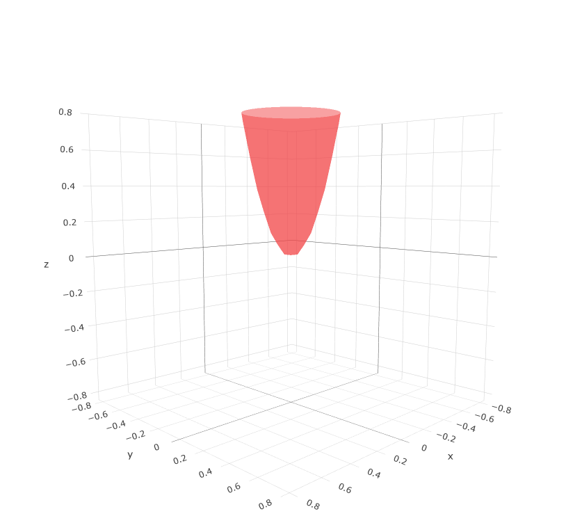

Right: The level set (see (2.14)) of the Lyapunov function constructed for the switched system (5.8) from Example 5.2. The orbital derivatives of the Lyapunov function were found and are negative in except for at the origin.
Remark 5.3.
Checking that the orbital derivative is negative was done by computing the values at the evaluation points. To obtain rigorous guarantees for the negativity you can either: use the form of obtained by meshfree collocation and Taylor-type estimates, similar to [11], or interpolate the function by a continuous piecewise affine (CPA) function, for which estimates can easily be checked, similar to [12].
6. Conclusion
In this paper, we have shown in Theorem 3.5 that the algorithm to construct a Lyapunov function for the switched system (2.1) originally presented in [21] converges under some specific assumptions. One such assumption is that the fill distance (3.13) decreases as the number of collocation points increases. In Section 3.4 we gave a way to choose collocation points so that the assumption on the fill distance is met. The construction method from [21] applies to both arbitrary switched and variable structure systems, as well as systems that have a combination of time- and state-dependent switching. We have provided further details on this method and given two new examples. Another main result is that the existence of a Lyapunov function for a switched system implies that the origin is a uniformly asymptotically stable equilibrium point of the system.
In Theorem 3.5 we also assumed the existence of a function . In future work, we will provide sufficient conditions for the existence of such a function.
References
- [1] R. A. Adams and J. J. Fournier, Sobolev Spaces, Elsevier, 2003.
- [2] R. Baier, L. Grüne and S. F. Hafstein, Computing Lyapunov functions for strongly asymptotically stable differential inclusions, IFAC Proceedings Volumes: Proceedings of the 8th IFAC Symposium on Nonlinear Control Systems (NOLCOS), Bologna, Italy, 2010, 1098-1103.
- [3] R. Baier, L. Grüne and S. F. Hafstein, Linear programming based Lyapunov function computation for differential inclusions, Discrete Contin. Dyn. Syst. Ser. B, 17 (2012), 33-56.
- [4] R. Baier and S. F. Hafstein, Numerical computation of control Lyapunov functions in the sense of generalized gradients, Proceedings of the 21st International Symposium on Mathematical Theory of Networks and Systems (MTNS), Groningen, Netherlands, 2014, 1173-1180.
- [5] M. S. Branicky, Multiple Lyapunov functions and other analysis tools for switched and hybrid systems, IEEE Trans. Automat. Control, 43 (2002), 475-482.
- [6] S. C. Brenner and L. R. Scott, The Mathematical Theory of Finite Element Methods, Springer, New York, 2008.
- [7] G. Davrazos and N. Koussoulas, A review of stability results for switched and hybrid systems, Proceedings of the 9th Mediterranean Conference on Control and Automation, Dubrovnik, Croatia, 2001.
- [8] P. Giesl, Construction of Global Lyapunov Functions using Radial Basis Functions, Springer, Berlin, Heidelberg, 2007.
- [9] P. Giesl, C. Argáez, S. Hafstein and H. Wendland, Construction of a complete Lyapunov function using quadratic programming, Proceedings of the 15th International Conference on Informatics in Control, Automation and Robotics (ICINCO), Porto, Portugal, 2018, 570-578.
- [10] P. Giesl, C. Argáez, S. Hafstein and H. Wendland, Minimization with differential inequality constraints applied to complete Lyapunov functions, Math. Comp., 90 (2021), 2137-2160.
- [11] P. Giesl and S. Hafstein, Computation and verification of Lyapunov functions, SIAM J. Appl. Dyn. Syst., 14 (2015), 1663-1698.
- [12] P. Giesl and N. Mohammed, Verification estimates for the construction of Lyapunov functions using meshfree collocation, Discrete Contin. Dyn. Syst. Ser. B, 24 (2019), 4955-4981.
- [13] P. Giesl and H. Wendland, Meshless collocation: Error estimates with application to dynamical systems, SIAM J. Numer. Anal., 45 (2007), 1723-1741.
- [14] S. F. Hafstein, An algorithm for constructing Lyapunov functions, Electron. J. Differ. Equ. Monogr., 8 (2007).
- [15] S. Hafstein, CPA Lyapunov functions: Switched systems vs. differential inclusions, Proceedings of the 17th International Conference on Informatics in Control, Automation and Robotics (ICINCO), Lieusaint-Paris, France, 2020, 745-753.
- [16] S. Hafstein, Sliding modes and Lyapunov functions for differential inclusions by linear programming, Proceedings of the 17th International Conference on Informatics in Control, Automation and Robotics (ICINCO), Lieusaint-Paris, France, 2020, 584-606.
- [17] W. Hahn, Stability of Motion, Springer, Berlin, Heidelberg, 1967.
- [18] L. Hou, A. N. Michel and H. Ye, Stability analysis of switched systems, Proceedings of the 35th IEEE Conference on Decision and Control, Kobe, Japan, 1996, 1208-1212.
- [19] H. K. Khalil, Nonlinear Systems, Prentice Hall, Upper Saddle River, New Jersey, 2002.
- [20] D. Liberzon, Switching in Systems and Control, Birkhäuser, Boston, Massachusetts, 2003.
- [21] J. Ward, N. Georgiou and P. Giesl, Construction of Lyapunov functions for switched systems using meshfree collocation, Proceedings of the 13th IFAC Symposium on Nonlinear Control Systems (NOLCOS), Reykjavík, Iceland, 2025, 49-54.
- [22] H. Wendland, Piecewise polynomial, positive definite and compactly supported radial functions of minimal degree, Adv. Comput. Math., 4 (1995), 389-396.
- [23] H. Wendland, Error estimates for interpolation by compactly supported radial basis functions of minimal degree, J. Approx. Theory, 93 (1998), 258-272.
- [24] H. Wendland, Scattered Data Approximation, Cambridge University Press, Cambridge, 2005.
- [25] K. Yosida, Functional Analysis, Springer, Berlin, Heidelberg, 2012.
- [26] V. I. Zubov, Methods of A. M. Lyapunov and their Application, US Atomic Energy Commission, 1961.