Optimal sequential two-stage Bayes Factor Design for two-arm clinical Phase II Trials with binary Endpoints
Abstract
Two-arm phase II clinical trials often benefit from an interim analysis that allows early stopping for futility, but Bayesian calibration of such designs is usually based on computationally intensive Monte Carlo simulation. In this work, a simulation-free methodology is developed to obtain Bayesian optimal two-stage designs in two-arm phase II trials with binary endpoints using Bayes factors as the primary measure of evidence. Building on recent matrix-search methods for fixed-sample two-arm Bayes factor designs and earlier correction formulas for one-arm two-stage designs, the proposed approach derives exact expressions for the operating characteristics of a two-stage two-arm design with a single futility interim. Bayesian power and type-I error are obtained by correcting the corresponding fixed-sample quantities for trajectories that would have been removed by early stopping, yielding a fully numerical calibration procedure that avoids Monte Carlo error entirely. The resulting method searches over admissible interim and final sample sizes to identify the optimal design that satisfies target constraints on Bayesian power, type-I error, and the probability of compelling evidence in favour of the null hypothesis, while minimizing the expected sample size under the null hypothesis. The methodology is illustrated in realistic phase II settings, including a detailed re-analysis of the riociguat trial in systemic sclerosis. Overall, the approach extends simulation-free Bayes factor design methodology to the practically important setting of two-arm two-stage phase II trials and provides a transparent basis for Bayesian design calibration and sensitivity analysis.
Keywords: phase II trial, sequential design, two-stage design, optimal trial design, Bayesian statistics, Bayes factors, two-arm clinical trial, binary endpoint
1 Introduction
Two-arm phase II clinical trials with binary endpoints are a central tool for assessing the preliminary efficacy of novel treatments before moving to larger, confirmatory phase III studies (6; 52; 16). Classical designs, such as Simon’s two-stage procedure, provide explicit frequentist control of type-I and type-II error rates and offer the option of early stopping for futility, thereby improving both ethical and efficiency properties compared to fixed-sample designs (51; 60). However, these methods typically do not incorporate prior information in a principled way and are not framed in terms of coherent Bayesian measures of evidence.
Bayesian designs address these shortcomings by allowing the formal inclusion of historical data, expert opinion, or mechanistic knowledge via prior distributions, and by updating beliefs as data accrue (2; 52; 56; 42). Decision rules are often based on posterior probabilities or Bayes factors, with the latter quantifying the relative support of the data for competing hypotheses in a way that is invariant to the prior odds on the hypotheses themselves (23; 25; 46; 59). As regulatory agencies increasingly encourage Bayesian analyses that demonstrate acceptable frequentist operating characteristics, so-called calibrated Bayes or Bayes–frequentist compromise approaches have gained prominence (7; 38; 15; 57; 21). For a recent guidance for industry issued by the Food and Drug Administration (FDA) on the use of Bayesian methodology in clinical trials, see 58.
In practice, however, Bayesian sample size planning and design calibration often rely on intensive Monte Carlo simulation studies. For a given Bayesian test statistic—such as a Bayes factor or a posterior probability—and a chosen decision threshold, power and type-I-error rates are typically evaluated by simulating many trial replicates under and (3; 47; 55; 16). This simulation-based paradigm raises several challenges:
- (i)
calibration becomes computationally expensive
- (ii)
reproducibility depends on reporting Monte Carlo standard errors and implementation details
- (iii)
every change in priors, thresholds, or design parameters may require re-running large simulations
There are several approaches available in the literature which either aim at reducing the computational burden associated with calibrating a Bayesian design or at least providing a calibrated Bayesian design, even if the computational effort often is substantial. A comprehensive review of Bayesian sequential clinical trial designs based on posterior and predictive probabilities, as well as decision‑theoretic criteria, is given by 61, who also discuss frequentist, calibrated Bayesian, and subjective Bayesian perspectives on interim monitoring and the likelihood principle.
In a related attempt to reduce the computational burden of calibrating Bayesian designs, 18 propose an efficient methodology for Bayesian clinical trials with clustered data that models posterior probabilities as functions of the number of clusters to assess operating characteristics across sample sizes from only a few simulation points.
Similarly, 62 propose a Bayesian sequential design for time‑to‑event outcomes that uses alpha‑spending functions to control the overall type‑I error rate and employs Bayes factors for interim decision‑making, illustrating that Bayes factor–based sequential monitoring can match or improve the efficiency of classical group sequential designs.
Another example is 13, who develop a Bayesian sequential decision‑making framework for rare disease trials with binary endpoints, combining sequential Bayes factor updates with adaptive stopping rules for superiority and futility to reduce expected sample size while maintaining interpretable evidence thresholds.
49 consider Bayesian group sequential designs for cluster‑randomized trials, proposing flexible schemes that allow early stopping for efficacy at pre‑planned interim analyses and exploring their operating characteristics via simulation for different recruitment patterns and outcome types.
However, all of these approaches rely on simulating the trial operating characteristics in one form or another, leading to the problems (i) to (iii) described above.
Recent work has shown that these obstacles can be overcome in important special cases. In the one-arm binomial setting, numerical root-finding and prior-predictive calculations allow for essentially instantaneous Bayesian power and sample size computations for Bayes factors, entirely avoiding Monte Carlo simulation (27). This approach has been extended to a Bayesian optimal two-stage design for single-arm phase II trials with binary endpoints, where a single interim analysis is accommodated via a trinomial-tree representation of the Bayes factor trajectories, and the resulting power and type-I error rates are analytically corrected for the possibility of early stopping (28). More recently, analogous matrix-search methods have been developed for two-arm binomial phase II designs, yielding simulation-free Bayesian power and sample size calculations for a broad class of Bayes factors in the two-arm setting (35). We provide details and summarize these approaches in Section 3.
Despite these advances, there is currently no simulation-free methodology for Bayesian two-arm phase II designs with both (i) Bayes factor-based decision rules and (ii) a formal two-stage structure allowing for a single interim analysis.11 1 A notable exception is the recent work of 44, who extend classical group sequential theory to Bayes factor designs by mapping Bayes factor stopping regions to z‑statistic boundaries, allowing fast, simulation‑free computation of stopping probabilities via multivariate normal integration. The approach proposed in this paper shares the same goal, in the sense that it is simulation-free but focusses on binomial endpoints. In contrast to the approach of 44, we do not map Bayes factor stopping regions to z-statistic boundaries. Also, no use of classical group sequential theory and its asymptotic arguments is made in this paper, which might in some cases become problematic in the context of a clinical phase II trial due to its limited sample size. The aim of this work is to fill this gap by combining the trinomial-tree correction ideas from the one-arm two-stage design with the matrix-search framework for two-arm Bayes factor calibration, thereby providing a fully numerical, simulation-free approach to Bayesian two-stage two-arm phase II trial design with binary endpoints.
2 Outline
The remainder of this manuscript is organized as follows. Section 3 reviews Bayesian power and sample size calculations for Bayes factors in binomial models, summarizing existing simulation-free results for one-arm fixed-sample designs, one-arm two-stage designs, and two-arm fixed-sample designs. Section 4 introduces the proposed two-stage two-arm Bayes factor design, detailing the construction of interim and final decision regions, the corresponding prior-predictive probabilities, and the correction of power and type-I-error for early stopping. We derive several main results, based on which Section 5 then presents the calibration algorithm for choosing interim and final sample sizes for an optimal Bayesian design under prespecified operating characteristics. Section 5 also discusses optimization criteria such as minimizing the expected sample size under the null hypothesis to classify a design as optimal from a Bayesian point of view. Section 6 illustrates the method in realistic phase II scenarios, and Section 7 concludes with a discussion of practical implications, limitations, and directions for future research.
3 Background
3.1 Bayes factors and calibrated Bayesian design
Bayes factors quantify the relative evidence provided by the data for two competing hypotheses and via the ratio of their marginal likelihoods (23; 25):
Interpreted as a predictive updating factor from prior to posterior odds,
| (1) |
Bayes factors separate the influence of the prior odds on the hypotheses from the influence of the parameter priors within each hypothesis. In particular, for a fixed pair of design and analysis priors on the model parameters, the Bayes factor reflects only how the data update relative support for vs. (59; 1; 30; 14; 26). This separation has been argued to make Bayes factors a more transparent index of evidence than posterior probabilities, especially when the prior odds on the hypotheses are themselves controversial or informed by historical information (16; 31; 37; 39; 32).
From a design perspective, Bayes factors can be used as test statistics for which frequentist-style operating characteristics such as power and type-I-error are defined in terms of exceedance probabilities of Bayes factor thresholds.22 2 This approach was championed by 14, who proposed it as a Bayes-frequentist compromise. Harold Jeffreys already suggested using what we now call Bayes factors as test statistics and studying their long‑run behavior in his 1939 monograph and subsequent editions of Theory of Probability (23). His methodology explicitly ties Bayes factors to error‑rate style criteria and proposes fixed thresholds (Jeffreys’ scale) in analogy to significance testing. Jack Good then developed this line further in the 1960s–1980s, discussing “weight of evidence” (essentially the logarithm of the Bayes factor) and emphasizing that Bayes factor–based tests can be judged by their long‑run frequencies of misleading evidence and related error probabilities. He is widely cited as an early advocate of calibrating Bayesian procedures (including Bayes factors) via long‑run error concepts. For an overview see 48. For example, using the orientation and an evidence threshold , one may define
| (2) | ||||
| (3) |
and require that these quantities satisfy inequalities analogous to classical design constraints for prespecified , such as
| (4) |
and
| (5) |
(27; 15; 16; 45). This Bayes–frequentist compromise is attractive for trial planners and regulators: it preserves a coherent Bayesian evidence measure while guaranteeing interpretable long-run error control (7; 38; 16; 21). This goes beyond the current recommendations and advice of regulatory agencies like the FDA or European Medicine’s Agency (EMA), compare 57; 58; 9.
3.2 Simulation-free Bayes factor calibration in the binomial setting
In most realistic models, the distributions of Bayes factors under and do not admit closed-form expressions, and power and type-I-error must be evaluated via Monte Carlo simulation (3; 47; 55). This is particularly true for adaptive or sequential designs, where the stopping rule and updating scheme introduce complex dependencies across interim looks (5; 61; 29). Simulation-based calibration, however, suffers from several drawbacks: it is computationally expensive, sensitive to the choice of simulation size and random seeds, and requires careful reporting of Monte Carlo standard errors and convergence diagnostics to ensure reproducibility (40; 4; 33).
In the one-arm binomial setting, 27 showed that these limitations can be circumvented. Focusing on tests of versus or directional alternatives, they derive Bayes factors under conjugate beta priors and obtain simple expressions for the prior-predictive distribution of the binomial count. Power and type-I-error are then written as sums of prior-predictive probabilities over sets of critical values determined by numerical root-finding on the Bayes factor. In other words, the Monte Carlo step is replaced by a direct evaluation of
where is the set of counts at which the Bayes factor crosses the evidence threshold . This approach leads to essentially instantaneous computation of Bayesian power and sample size in the binomial setting, without any simulation and without relying on asymptotic approximation. It is implemented in the R package bfbin2arm as well as in the R package bfpwr (43).

3.3 One-arm two-stage Bayes factor designs via trinomial-tree branching
Building on this root-finding framework, 28 proposed a Bayesian optimal two-stage design for single-arm phase II trials with binary endpoints based on Bayes factors. The design introduces a single interim analysis after patients, with the option to stop early for futility if the Bayes factor indicates strong evidence in favour of . The novelty lies in showing how to correct the Bayesian power and type-I-error rate for the presence of this interim look, again without resorting to Monte Carlo simulation.

The key device is a trinomial-tree representation of the Bayes factor trajectories: at each analysis (interim and final), the Bayes factor can indicate efficacy (evidence for ), futility (evidence for ), or be inconclusive, compare Figure 2. In Figure 2, denotes the data available in the treatment and control group at interim analysis and the Bayes factor based on the available interim data. The tupel denotes the full trial data available at the end of the trial and the Bayes factor based on this full trial data. We introduce the setup and notation in detail in Section 4.1.33 3 In 28, the one-arm setting with only a treatment group is considered, so there the Bayes factors are based on treatment group data only. Here, we consider the two-arm phase II setting with a treatment and control group, and modified notation and Figure 2 accordingly.
When the design is naively calibrated using the fixed-sample expressions at alone, trajectories that would have stopped for futility at the interim but later “swing back” to evidence for at the final analysis are incorrectly counted as contributing to power (and analogously for type-I-error under ). The authors identify these trajectories as a “futility-erased partial power” (and “futility-erased partial type-I-error”) and provide closed-form summation formulas, using prior-predictive distributions, to subtract these contributions from the fixed-sample power and type-I-error (28). This yields corrected operating characteristics for the two-stage design that account exactly for the possibility of early stopping, while preserving the simulation-free nature of the calibration.
In terms of Figure 2, this corresponds to the lowest blue trajectory: Without an interim analysis, the Bayes factor could indicate futility when calculated based on the interim sample size , and then swing back to reach efficacy in the final analysis. These trajectories contribute to Bayesian power when no interim analysis is carried out. Once an interim analysis is introduced, however, the trial can be stopped when the futility threshold is reached at the interim sample size, reducing the power by “cutting off” the possibility that the Bayes factor swings around and reaches efficacy for the final sample size at the end of the trial in these trajectories.
In addition to the correction the authors propose to solve this problem, 28 develop a calibration algorithm that searches to find Bayesian optimal two-stage designs that
- (i)
satisfy prespecified constraints on Bayesian power and type-I-error, compare Equation 5 and Equation 4, and
- (ii)
minimize the expected sample size under . The resulting design thus is computed as the result of the following optimization problem:
(6)
where is the Bayes factor based on the final sample size at the end of the trial. The resulting designs recover Simon-type optimal designs as special cases, improve non-sequential Bayes factor designs, and can be calibrated rapidly using only standard numerical methods.44 4 The calibration algorithm for the two-stage single-arm design is currently implemented in the bfbin2arm R package (35), available on CRAN under https://cran.r-project.org/web/packages/bfbin2arm/index.html. 27 call such a design optimal in the Bayesian sense.
3.4 Two-arm fixed-sample designs via matrix search
35 extended the root-finding approach to the two-arm binomial setting, accommodating a variety of hypotheses relevant for two-arm phase II trials, including equality of response probabilities vs. ), superiority ( vs. – where ) denotes the difference in success probabilities between the treatment and control arm – and ordered alternatives. The corresponding Bayes factors is derived there under flexible beta design and analysis priors as well as the joint prior-predictive distribution of the binomial counts in the two arms, , in closed form.
The key insight is that the discrete nature of the binomial counts reduces the problem to a finite matrix search over all integer pairs . For fixed sample sizes in the control and treatment arms and a chosen evidence threshold , one first computes the Bayes factor at every lattice point. The efficacy region—the set of count pairs that provide evidence against —is then
Figure 3 illustrates this procedure for and flat analysis priors (). The left panel shows the matrix of Bayes factors , where rows index the number of control arm successes and columns index treatment arm successes . As expected under the two-sided test vs. , the matrix is symmetric around the main diagonal (), with largest values (strongest evidence for ) along this diagonal and progressively smaller values toward the top-right and bottom-left margins (evidence against ).
 (a) Bayes factors
|
(b) Critical region: |
 (c) Prior-predictive under
|
The middle panel (b) identifies the critical efficacy region by setting all entries where to zero, leaving only those lattice points that would lead to rejection of . In this example,
Finally, the right panel (c) shows the prior-predictive probabilities under a chosen design prior, restricted to . The Bayesian power is simply the sum of these probabilities:
The type-I-error rate under is computed analogously by summing over the same region .
This matrix-search approach completely replaces both numerical root-finding (one-arm case) and Monte Carlo simulation with direct enumeration of the finite sample space. Sample size determination proceeds by repeating the procedure for increasing until the desired power and type-I-error bounds are achieved. The methodology is implemented in the bfbin2arm R package, enabling rapid exploration of two-arm Bayes factor designs with a treatment and control group across a wide range of hypotheses, priors, and thresholds (35).
3.5 Motivation for a two-arm two-stage Bayes factor design
The three strands of work described above establish a coherent simulation-free framework for Bayes factor-based designs in (i) one-arm fixed-sample binomial trials (27), (ii) one-arm two-stage trials via trinomial-tree branching and futility-erased corrections (28), and (iii) two-arm fixed-sample binomial trials via matrix search (35). Together, they demonstrate that Bayesian designs with Bayes factor decision rules can be calibrated numerically, without Monte Carlo simulation, while maintaining interpretable Bayesian and frequentist properties.
In many phase II settings, however, the combination of a control and treatment arm and interim monitoring is highly desirable. Two-arm designs offer a more realistic assessment of treatment effect by directly comparing a novel treatment to standard of care or placebo, while two-stage designs with an interim futility analysis reduce expected sample size under and limit exposure to ineffective therapies (51; 60; 3). Existing Bayesian two-arm designs with interim analyses usually rely on simulation-based calibration and often do not use Bayes factors as the primary decision criterion (10; 11; 54; 12).55 5 Nothing is requiring to use Bayes factor as the test statistic for assessing the hypotheses under consideration in the previous work outlined in Section 3. Here, we focus on using Bayes factors due to their advantages as a measure of statistical evidence. For a detailed treatment of the advantages and limitations of various measures of statistical evidence see 53. The important implication for the methodology developed in the current manuscript is that one could use all of the power and sample size calculation methodology developed so far and adjust the measure of statistical evidence to e.g. posterior probabilities or posterior odds. This would allow to apply the current methodology developed in this paper also to these measures of statistical evidence, yielding optimal designs which are based on e.g. posterior probabilities or posterior odds of the competing hypotheses.
The natural next step, therefore, is to combine the trinomial-tree correction ideas of the one-arm two-stage Bayes factor design with the matrix-search framework of the two-arm fixed-sample design. Conceptually, this entails moving from (i) a one-dimensional count of successes in a single arm to (ii) a two-dimensional grid of successes in two arms, and from (iii) a two-dimensional sum over interim and final counts in the one-arm case to (iv) a four-dimensional sum over interim and incremental counts in the two-arm case. The same logic applies: identify the set of trajectories that would be cut off by an interim futility stopping rule but that would otherwise contribute to fixed-sample power or type-I-error, and subtract their prior-predictive probabilities from the naive fixed-sample operating characteristics.
By doing so, one can derive a simulation-free, Bayes factor-based two-stage design for two-arm phase II trials with binary endpoints that:
- •
Controls Bayesian analogues of type-I-error and power at prespecified levels, in a way that is interpretable from both Bayesian and frequentist perspectives, compare Equation 4 and Equation 5.
- •
Admits explicit numerical corrections for the interim futility analysis via sums of prior-predictive probabilities, avoiding Monte Carlo simulations.
- •
Allows optimization criteria such as minimal expected sample size under , generalizing the notion of Bayesian optimal two-stage designs to the two-arm setting, compare Equation 6.
The remainder of this work develops exactly this extension, showing how the trinomial-tree branching concept and futility-erased partial contributions can be generalized to the two-arm matrix-search setting in order to obtain an optimal two-stage two-arm Bayes factor design. The most relevant application of such an extension is a phase II clinical trial with a treatment and control arm and a primary binary endpoint.
4 Extending the Two-Arm Bayes Factor Design to a Two-Stage Setting
In this section, we outline how to extend the fixed-sample two-arm Bayes factor design for phase II trials with binary endpoints detailed in 35 to a two-stage design with a single interim analysis. The goal is to retain the simulation-free calibration philosophy: power and type-I-error are obtained by summing prior-predictive probabilities over suitable regions in the sample space, now taking into account the option to stop early for futility.
4.1 Setup and notation
We consider a two-arm trial with a control group () and a treatment group (). Let denote the planned total sample size in arm at the final analysis, and let denote the sample size in arm at the interim analysis. For simplicity, we assume that the allocation ratio is fixed and that the interim occurs after and patients have been observed in the control and treatment arm, respectively. We denote by
the numbers of successes in arm in the first and second stage, respectively. The final totals are
Thus describes the interim data and the final data, if the trial is continued to the second stage.
As in the two-arm fixed-sample setting, we write and for the null and alternative hypotheses of interest. In a phase II trial, two hypotheses are typically of interest. One tests equality of response probabilities in treatment and control, , where the former receives the novel drug and the latter standard of care or placebo:
| (7) |
A convenient reparameterization introduces the difference and the grand mean , so that
and the hypotheses become
| (8) |
This parameterization originates from 17 and has been used in subsequent work, see also 8, 22 and 34. In a phase IIb setting, testing is attractive because it allows explicit evidence for equal efficacy of novel treatment and control. If evidence instead supports , either (control more effective than treatment) or (treatment more effective than control) may occur, and estimating and post-hoc should supplement this hypothesis test for a more complete interpretation.
An alternative is to use directional tests:
| (9) | ||||
| (10) | ||||
| (11) |
In the first, states that placebo or standard of care is at least as effective as the novel treatment, while asserts superior efficacy of the novel treatment. The one-sided test with versus assumes (i.e., ) is a priori unrealistic, for example when the control arm receives standard of care and the treatment arm receives standard of care plus a non-interfering add-on, so the treatment success probability should be at least as large. Conversely, the one-sided test with versus is relevant when the endpoint measures failures; ruling out a priori implies , which is reasonable if the control group receives standard of care and the treatment group standard of care plus an add-on that cannot worsen outcomes.
35 uses conjugate beta design priors under each hypothesis, developed for the two-sided Bayes factor test
The beta–binomial model then yields closed-form prior-predictive probability mass functions
| (12) |
| (13) |
and
| (14) |
for . Under , the arms receive independent beta design priors,
and the prior-predictive probability mass function for interim data under the two‑sided test, with interim sample sizes and , is
for , . Under the null hypothesis , the common parameter follows a beta prior , so the corresponding joint prior-predictive probability mass function for the arm-wise interim totals is
for , . This joint probability mass function governs the distribution of the interim data under and is used in the calculation of the type-I-error probabilities. For computational purposes, the Bayesian power and type-I-error probabilities are obtained by summing the prior-predictive probability mass function over all that fall into the respective critical regions.
The probability mass function
for the final-sample arm-wise counts is precisely the two-arm prior-predictive distribution already used in the fixed-sample Bayes factor sample size calculations for the two-sided test versus , with final sample sizes and and, potentially, different design-prior parameters. The only difference compared to the interim probability mass function is that the counts now refer to the final totals and the corresponding final sample sizes, rather than the interim sizes. All these prior-predictive probability mass functions are later used to compute the Bayesian power and type-I-error probabilities under the respective design priors.
In closing this subsection, we note that we only detail the derivations for the two-sided test of versus , but the prior-predictive probability mass functions and the corresponding Bayes factors for the above directional tests have been derived by 35. The general approach outlined for the two-sided test can therefore easily be extended to the directional tests, which are often more relevant in the context of a phase II trial. For the directional tests, the beta design and analysis priors change to truncated versions on the parameter spaces associated with and , and the prior-predictive probability mass functions do likewise. For details, also on the resulting Bayes factors for these directional tests, we refer to the Appendix of 35.
4.2 Bayes factors at interim and final analysis
Let denote the Bayes factor in favour of based on the interim counts , and the Bayes factor based on the final totals . These are exactly the two-arm Bayes factors derived in the fixed- two-arm setting, now evaluated at the interim and final sample sizes. We choose two thresholds:
- •
for evidence against (efficacy boundary).
- •
for evidence in favour of (futility boundary).
Using the orientation, a small Bayes factor ( for e.g. or ) indicates evidence against in favour of , while a large Bayes factor () indicates evidence for .66 6 This is in line with the interpretation of p-values, simplifying the use and interpretation for frequentists. At the interim analysis, we define:
The interim efficacy region is optional, as it only becomes relevant when stopping for efficacy after the interim analysis is allowed for. In our current design, this is not the case but we briefly explain how a possible extension could look like in Section 4.6 below. At the final analysis, we define the final efficacy region
We focus on the case where early stopping is allowed only for futility.
4.3 Unadjusted (fixed-sample) operating characteristics
Ignoring the interim look and treating the design as fixed-sample with total sample sizes and , the Bayesian analogues of type-I-error rate and power are given by
The quantity is the naive Bayesian type-I-error rate, whereas is the naive Bayesian power. These are the quantities used in the fixed-sample two-arm Bayes factor sample size calculations, compare 43, 27; 28 and 35.
However, once we introduce the option to stop early for futility at the interim analysis (i.e. whenever ), these unadjusted probabilities overestimate the true power and type-I-error rate of the resulting two-stage design, for the same reason as in the single-arm two-stage setting: some data trajectories that would have contributed to are no longer possible because the trial would have been stopped early.
4.4 Futility-erased partial power and type-I-error
The key idea is to identify those trajectories that (i) would have stopped for futility at the interim analysis, but (ii) would have produced a final Bayes factor indicating efficacy if the trial had continued to the second stage. In the single-arm two-stage setting, these trajectories gave rise to the so-called “futility-erased partial power” and “futility-erased partial type-I-error”, which must be subtracted from and , respectively. We now derive the two-arm analogue.
Lemma 1.
For a given hypothesis (), the joint prior-predictive distribution of factorizes as
where and are the stage-wise prior-predictive probability mass functions in Equation 12 and Equation 13.
Proof.
See the Appendix. ∎
Based on Lemma 1, one can derive the following two-arm analogue of the futility-erased partial contribution to Bayesian power or type-I-error rate for a two-arm sequential two-stage design with binary endpoints in both groups:
Theorem 1.
The two-arm futility-erased partial contribution for hypothesis , to Bayesian power or type-I-error rate is given as follows:
Proof.
See the Appendix. ∎
In Theorem 1, the inner sum runs over all second-stage increments that, together with a futility-interim pair , would have led to a final total in the final efficacy region . In the context of Figure 2, corresponds to the probability of the lowest of the three blue trajectories. If , it is the futility-erased partial contribution to the Bayesian type-I-error rate of the resulting two-stage design. If , it is the futility-erased partial contribution to the Bayesian power of the resulting two-stage design.
Intuitively, is a two-arm, four-dimensional version of the “futility-erased partial power” described in the trinomial-tree framework of 28 for the single-arm two-stage design. It collects exactly those trajectories that are counted in the fixed-sample power or type-I-error, but are no longer reachable when the trial is stopped for futility after the interim analysis.
In the Appendix, we provide another version of Lemma 1 and Theorem 1 which prove the factorization and double-sum expression also for the directional tests given in Equation 17 to Equation 19.
4.5 Corrected operating characteristics for the two-stage two-arm design
The corrected Bayesian type-I-error rate and power of the two-stage design with a single futility interim are obtained by subtracting the futility-erased partial contributions from the naive fixed-sample probabilities:
Here, is the corrected Bayesian type-I-error rate, whereas is the corrected Bayesian power. In the simplest case with early stopping only for futility (no early efficacy stopping), the second equation reduces to
because all trajectories contributing to efficacy must go through the final analysis and those that would have stopped for futility but later yielded efficacy are precisely the ones counted in .
If early stopping for efficacy at the interim analysis is allowed (see Section 4.6 below), the expression for includes an additional term for interim efficacy.
4.6 Extension to early stopping for efficacy
If early stopping for efficacy at the interim analysis is allowed,
and the decision rule gains a second type of early stop: in addition to futility, the trial may stop when with . In this case, the overall Bayesian power under decomposes into
where is the Bayesian power in the fixed-sample design, is the futility-erased partial power (paths in the futility region that would have fallen into the final efficacy region had the trial continued, corresponding to the lowest blue trajectory in Figure 2), and is the analogous efficacy-erased partial power (paths in the efficacy region that would have also satisfied the final efficacy rule but are now counted only once, in the first summand. As they are included both in the first summand and , they must be subtracted once. The corresponding path is the upper blue trajectory in Figure 2.). The first term accounts for trajectories stopped for efficacy at the interim, while the bracketed term corresponds to the probability of declaring efficacy at the final analysis, after correcting for both erased trajectories which are “cut off” because one stops for futility or efficacy. Under , analogous decompositions can be derived for the type-I-error rate, and the calibration algorithm outlined in the following subsection could proceed along the same lines, with the additional constraint that early efficacy contributions must be included in the power and type-I-error targets. In this paper, we solely consider stopping early for futility, but future research could deal with extensions involving designs which allow early stopping for efficacy.
4.7 Corrections for the probability of compelling evidence for the two-stage two-arm design
Next to the power and type-I-error, another operating characteristic of the trial design which changes when introducing an interim analysis is the probability of compelling evidence
where the calibration requires the latter to achieve at least a minimum probability :
In principle, for a given final sample size the corrected two-stage probability of obtaining compelling evidence for , denoted , may exceed its fixed-sample counterpart associated with the same totals. The reason is that, in the two-stage design, interim outcomes that fall into the futility region are counted immediately as compelling evidence for , whereas in the corresponding fixed-sample design the trial would necessarily continue to the final analysis before is assessed. As shown in the appendix, therefore decomposes into the sum of the probability of early futility stopping and the probability of reaching compelling evidence for at the final analysis after continuation, which implies that , with strict inequality whenever some interim futility outcomes would not lead to compelling evidence for in the fixed-sample design.
In the calibration algorithm described in the following section, the constraint on is nevertheless enforced already at the fixed-sample level in Step 1. This should be viewed as a conservative feasibility screen: by requiring the fixed-sample design to attain the desired probability of compelling evidence for , Step 1 tends to exclude unrealistically small final sample sizes for which even the non-sequential fixed-sample procedure cannot meet the evidence requirement. In Step 2 of the calibration algorithm detailed in the following section, the constraint is then checked again using the corrected two-stage quantity for each candidate interim design. Thus, Step 1 of the calibration algorithm detailed next provides a conservative screening device, while the final calibration of the sequential design is based on the corrected two-stage operating characteristics derived in Appendix B.
5 Calibration algorithm in the two-arm two-stage setting
The calibration problem now is to choose interim and final sample sizes such that the corrected operating characteristics satisfy prespecified bounds, e.g.
| (15) |
and optionally a constraint on the probability to stop for futility under ,
| (16) |
The probability to stop for futility under above quantifies the chance that the interim data provide compelling evidence for and the trial is stopped early. A closely related idea appears in the Bayesian reanalysis of null results by 20, who refer to “compelling evidence for the null hypothesis” when Bayes factors exceed a fixed threshold. In the context of Bayesian group‑sequential and phase II designs, early stopping rules for futility are studied using Bayesian posterior or predictive probabilities; examples and discussions of such rules and their operating characteristics can be found in 19 and in the tutorial on modern Bayesian methods in clinical trials by 41, as well as 24. In what follows, we use the term compelling evidence for , in line with 27, 28 and 35.
A natural calibration algorithm based on Lemma 1 and Theorem 1, which mirrors the single‑arm two‑stage design, is now given as follows.
- 1.
Step 1 (fixed-sample calibration): For a fixed allocation ratio, search over a grid of total sample sizes with , for a realistic range of minimum and maximum sample sizes and , until the naive fixed-sample Bayesian power exceeds a prespecified target (e.g. 80%), possibly with a small cushion (e.g., for a small ). This yields a “sufficient” full-trial size.
- 2.
Step 2 (two-stage calibration): For the chosen full-trial size, search over interim sample sizes and identify those designs that satisfy the constraints on the corrected operating characteristics and in Equation 15, as well as any optional constraint on the probability of early stopping for futility under in Equation 16. Among these, select the design that optimizes the desired criterion, e.g., minimizes the expected total sample size under .
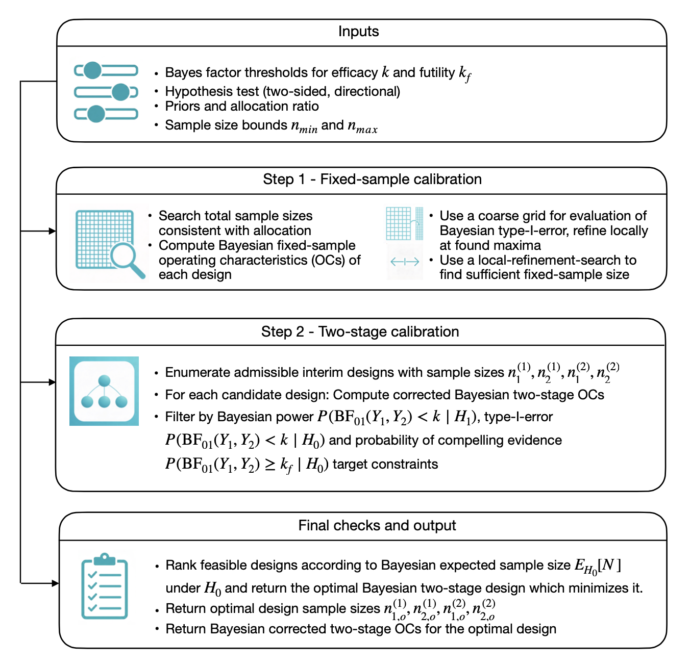
Figure 4 visualizes the calibration algorithm for finding an optimal Bayesian two-arm two-stage design. Note, that nothing requires to use Bayes factors after all. One could also use posterior probabilities or any other test statistic and proceed likewise, replacing the computation of Bayes factors with the other test statistic of choice.
Now, if no such design is found, the full-trial size can be increased and the process repeated. The resulting algorithm in detail then looks as follows.
- 1.
Input: Design and analysis priors under and , Bayes‑factor thresholds and , target error bounds , allocation ratio, hypotheses to test and (optionally) a target probability of early stopping for futility under .
- 2.
Find a sufficiently large fixed‑sample size: For an increasing grid of total sample sizes with for (e.g. constrained by a fixed allocation ratio), compute the naive fixed‑sample Bayesian power
until it exceeds the target , possibly with a small cushion (e.g., up to for a small ).77 7 This step ensures that the resulting Bayesian power target can be reached in principle. Based on Theorem 1, the power in the two‑stage design can only decrease when an interim analysis that allows stopping for futility is introduced. As a consequence, if the fixed‑sample design cannot reach the target power, no two‑stage design with that or smaller total sample size can. This computation is performed by means of the matrix‑search algorithm outlined in Section 3.4. Optionally, compute the naive fixed-sample probability of compelling evidence and calibrate it according to Equation 16.88 8 Note that for screening for a sufficient fixed-sample size, we do not use as defined in Equation 20, which is the corrected two-stage probability of compelling evidence. We solely use the fixed-sample probability of compelling evidence, as the corrected two-stage probability of compelling evidence must increase when introducing an interim analysis which allows stopping for futility. See Appendix Section B.1. Let denote a candidate full‑trial size that achieves this (or lies in a small surrounding region).
- 3.
Compute fixed‑sample type‑I‑error at that size: For the chosen total sample size , compute the corresponding naive fixed‑sample type‑I‑error
where .99 9 Note that the type-I-error rate also can only decrease when introducing an interim analysis which allows to stop for futility only. As a consequence, even if the resulting type-I-error rate for that sample size does not meet the desired requirements, the resulting two-stage design can still meet those.
- 4.
Iterate over interim sample sizes: For the fixed final sample size pair , consider candidate interim sample size pairs 1010 10 For example, as fractions of , or starting from a small value such as , iterating up to for balanced randomization, and analogously for non‑balanced randomization.:
- (a)
Compute the stage‑wise prior‑predictive probability mass functions and for .1111 11 The prior‑predictive probability mass functions for the two‑sided and directional tests are available in the Appendix of 35. For the two-sided test, see also Equation 12 and Equation 13.
- (b)
Identify the interim futility region and the final efficacy region by evaluating the Bayes factor at all possible combinations of and .1212 12 All Bayes factors for the two‑sided and directional tests are available in the Appendix of 35 and can be computed via standard numerical integration.
- (c)
- (d)
Obtain the corrected operating characteristics
- (e)
Compute the probability of early stopping for futility under :
and the expected total sample size under :
where and .
- (a)
- 5.
Design selection: Among all interim‑size pairs for the fixed total size that satisfy the constraints
and (optionally) with as defined in Equation 20, choose the one that minimizes (or some other desired criterion) and call it the Bayesian optimal two‑stage design, in line with the notation in 28.
- 6.
If no such design exists: Increase the final sample size and repeat steps 2–5 until a design is found that satisfies all constraints.
In line with the fifth step of selecting an optimal design among all trial designs which fulfill the required conditions on Bayesian type-I-error rate and power, we formally define the optimal two-arm two-stage Bayes factor design (for binary endpoints) as follows:
Definition 1 (Optimal two-arm two-stage Bayes factor design for binary endpoints).
Let and be given, and let denote the minimum interim sample sizes at which the trial may stop for futility, and let denote the maximum final sample sizes. For a given Bayes-factor threshold , the optimal two-arm two-stage Bayes factor design for binary endpoints is any admissible design that solves
subject to
where is defined in Equation 20, and
Here, and denote the corrected Bayesian type-I error and power of the two-stage design, and the corrected probability of compelling evidence of the two-stage design.
The algorithm is implemented in the R package bfbin2arm, which is available on CRAN.1313 13 The package and various vignettes illustrating the use are available under https://cran.r-project.org/web/packages/bfbin2arm/index.html.
6 Examples
6.1 Re-analysis of the Riociguat phase II trial in systemic sclerosis
To illustrate the proposed methodology, we reconsider the riociguat phase II trial in systemic sclerosis discussed in the fixed-sample two-arm Bayes factor design setting by 35, compare also 36.1414 14 A detailed software vignette including all relevant R code to recreate this example which also includes further explanations is available on CRAN. The example is attractive because it represents a realistic two-arm phase II setting with a binary endpoint, while also showing that the practical behaviour of the proposed two-stage calibration algorithm depends strongly on the prior-predictive separation of the competing hypotheses.
Let denote the response probability in the control arm and the response probability in the treatment arm. In the riociguat example, the observed response rates are
Since the observed response rate is higher in the treatment arm, we consider the one-sided superiority setting
implemented through the Bayes factor , that is, evidence against corresponds to small values of the Bayes factor in favour of the null.
Throughout this example, the efficacy and futility thresholds are chosen as
Thus, efficacy is declared when the Bayes factor falls below , whereas compelling evidence in favour of the null hypothesis is declared when the Bayes factor is at least . We calibrate the design to satisfy a Bayesian type-I-error bound of , Bayesian power , and a lower bound of on the probability of compelling evidence for .
Priors.
We distinguish between design priors, which determine the prior-predictive operating characteristics used during calibration, and analysis priors, which enter the Bayes factor itself. For the riociguat example, we use a flat design prior under ,
and slightly informative design priors under ,
The corresponding analysis priors are chosen to be flat,
This choice reflects the intended separation between planning and analysis: prior information is allowed to influence the calibration of the design, but the eventual evidential assessment through the Bayes factor is based on neutral analysis priors.

One-stage reference design.
Before constructing the two-stage design, it is helpful to inspect the corresponding fixed-sample reference design obtained under the same calibration targets. Figure 5 shows the one-stage design calibrated to 80% Bayesian power, 2.5% Bayesian type-I error, and 60% probability of compelling evidence, and requires patients in total, corresponding to approximately to 27 patients per arm. At this sample size, the Bayesian power is about , the Bayesian type-I error is about , and the probability of compelling evidence in favour of is about .
The corresponding one-stage design is useful as a benchmark, but it does not permit early stopping for futility. The practical question is therefore whether an interim analysis can be introduced without materially damaging the operating characteristics.
Two-stage design with mildly informative design priors.
We now apply the proposed optimal two-stage calibration algorithm. The search is carried out under balanced randomization, with minimum interim sample sizes of 10 patients per arm and maximum final sample sizes of 80 patients per arm. Under the prior specification given above, the fixed-sample calibration step identifies a sufficient one-stage anchor with
Conditional on this anchor, the second step of the algorithm searches over admissible interim sample sizes and selects the design minimizing the expected total sample size under .

Figure 6 shows the results of the calibration algorithm.1515 15 See also the software vignette available at https://cran.r-project.org/web/packages/bfbin2arm/vignettes/bfbin2arm-twostage.html for details on how to recreate the results and plots with the bfbin2arm R package. For the riociguat example, the resulting optimal two-stage design is
Hence, the interim analysis is conducted after patients in total, and the maximal sample size is . The corrected operating characteristics of this design are
with early stopping for futility under occurring with probability about . The corresponding expected sample size under is
Several aspects are noteworthy. First, the corrected Bayesian power and type-I error remain comfortably within the desired design targets. Second, the price of allowing early futility stopping is small in terms of maximal sample size: the two-stage design increases the maximal sample size from in the one-stage reference design to , but preserves the intended operating characteristics. Third, the actual gain in expected sample size under is modest, because the futility stopping probability is only around . Thus, in this specific example, the interim analysis is feasible and principled, but it does not lead to a dramatic efficiency gain by itself.
Interpretation.
The modest reduction in is not a deficiency of the algorithm. Rather, it is a consequence of the joint calibration constraints. The efficacy threshold is fairly stringent, the futility threshold requires non-trivial evidence in favour of , and the additional requirement limits how aggressively null trajectories can be truncated at the interim analysis. Under such constraints, only a relatively small subset of null trajectories can be stopped early without compromising power or the evidence requirement for the null.
This example therefore illustrates an important practical point. A two-stage design does not automatically imply a substantially smaller expected sample size under . If the design priors under and are only moderately separated and the evidential thresholds are strict, then the calibrated futility rule may have only a limited opportunity to remove null trajectories early.
Two-stage design with more informative design priors.
To investigate the effect of stronger prior-predictive separation, we keep the analysis priors and Bayes factor thresholds unchanged, but replace the design priors under by the more informative specification
This modification leaves the eventual Bayes factor analysis unchanged; it only affects the calibration stage by expressing a more concentrated prior expectation that the control arm has relatively low response probability and the treatment arm relatively high response probability.

Figure 7 shows the results. Under this more informative design prior, the fixed-sample calibration step now identifies a sufficient one-stage anchor with
so that the corresponding maximal total sample size is . The optimal two-stage design becomes
Its corrected operating characteristics are approximately
with futility stopping probability under again close to , and expected sample size
The striking feature is that the futility stopping probability changes very little, whereas the expected sample size under decreases substantially, from about to . The reason is that the more informative design priors separate the predictive distributions under and much more clearly. As a result, the fixed-sample anchor from Step 1 becomes much smaller, and the resulting two-stage design inherits this smaller overall scale. In other words, in this class of examples, the main efficiency gain is not driven by making the interim rule dramatically more aggressive, but by reducing the total sample size needed for the competing hypotheses to become distinguishable under the design priors.
Comparison of the three designs.
Table 1 summarizes the key operating characteristics of the one-stage reference design and the two calibrated two-stage designs. The comparison highlights two complementary messages. First, the proposed two-stage procedure can reproduce the desired Bayesian operating characteristics while incorporating an interim futility analysis. Second, the practical efficiency of the resulting design depends strongly on the design-prior specification used for calibration.
| Design | Power | Type-I error | ||||||
|---|---|---|---|---|---|---|---|---|
| One-stage design | – | – | 27 | 26 | 53 | 0.80 | 0.0070 | 53.0 |
| Two-stage, mildly informative priors | 10 | 10 | 34 | 34 | 68 | 0.833 | 0.0058 | 66.04 |
| Two-stage, more informative priors | 10 | 10 | 13 | 13 | 26 | 0.853 | 0.0079 | 25.76 |
Overall, the riociguat example illustrates the central practical features of the proposed method. The algorithm provides a fully numerical, simulation-free calibration of Bayesian two-stage two-arm designs; it yields interpretable operating characteristics in terms of Bayes factor evidence thresholds; and it makes transparent how prior assumptions at the design stage influence both feasibility and efficiency. At the same time, the example also shows that early stopping for futility is not automatically associated with large savings in expected sample size. Whether such savings materialize depends crucially on how well the design priors separate the hypotheses under consideration.
In the riociguat example, the optimal two-stage design only stops early for futility under with probability about , so the reduction in the expected sample size under is very modest. This behaviour is not a bug of the algorithm, but a consequence of the modelling choices and calibration constraints.
First, the design is calibrated to fairly strict evidence requirements: the success threshold , the null-evidence threshold , the Bayesian type-I error bound , and the requirement together imply that only a small fraction of outcomes can be eliminated safely at the interim look without compromising either power or the probability of compelling evidence in favour of . Under such constraints, the interim boundary cannot be very aggressive, so the early stopping probability under remains low and stays close to the maximum sample size.
Second, even when the interim fraction is moved and the target is varied, the futility probability in this example is relatively insensitive as long as the thresholds and and the overall calibration targets remain fixed. Moving the interim later increases the information available at the interim, but the futility rule still has to preserve about 80% Bayesian power and the constraint, which limits how many null paths can be stopped early. In particular, with already fairly liberal for declaring evidence in favour of , further gains in early stopping would require relaxing this threshold in a way that is not clinically desirable here.
Third, the design priors have a pronounced effect on the expected sample size under . When the design priors under are made more informative and more clearly separated from , the predictive distributions under and diverge more quickly as the sample size grows. This leads to a smaller sufficient fixed-sample size and, consequently, to a smaller expected sample size under in the corresponding two-stage design, even if the interim futility probability itself changes only marginally. In the riociguat example, this can be achieved by concentrating the design priors slightly more around the clinically relevant success rates, while keeping the analysis priors and Bayes factor thresholds unchanged.
6.2 Riociguat trial re-analysis with slightly informative design priors
We revisit the riociguat phase II trial, this time using less optimistic but still slightly informative design priors. This second example illustrates how the necessary sample sizes are influenced by the design prior choice and how the sample size reduction of the optimal two-stage design compared to the calibrated one-stage design varies with different design prior choices. In contrast to the first example, we not require 90% Bayesian power instead of only 80%. The type-I-error (Bayesian) is again calibrated to 2.5%, and no minimum probability on compelling evidence in favour of is required.
Priors.
We now use a slightly informative design prior under ,
and slightly informative design priors under ,
encoding the expectation that the control arm has a lower response probability than the treatment arm. The corresponding analysis priors are chosen to be flat,
This choice reflects the intended separation between planning and analysis: prior information is allowed to influence the calibration of the design, but the eventual evidential assessment through the Bayes factor is based on neutral analysis priors.
One-stage reference design.
As a benchmark, we first consider the fixed-sample one-stage design obtained under the same thresholds and Bayesian calibration targets. Under the priors specified above and balanced allocation between arms, the one-stage calibration identifies a design with a total sample size of
patients, corresponding to 77 patients in each arm. At this sample size the Bayesian power is approximately , the Bayesian type-I error under is about , and the probability of compelling evidence for is about . This directly calibrated one-stage design serves as a reference for evaluating the corresponding two-stage design. The results are shown in Figure 8.

Two-stage design without power cushion.
We now apply the proposed two-stage calibration algorithm. The design includes a single interim analysis that allows early stopping for futility and is calibrated to the same Bayesian power and type-I-error targets as the one-stage design. Also, no calibration of the compelling evidence in favour of is carried out. The efficacy and futility thresholds and and the priors are kept unchanged.
Under these settings, the fixed-sample calibration step identifies a sufficient one-stage anchor with
corresponding to a total sample size of . At this anchor the Bayesian power under the design priors is approximately , the Bayesian type-I error is about , and the Bayesian probability of compelling evidence for is about . Conditional on this anchor, the second step of the algorithm searches over admissible interim sample sizes and selects the design that minimizes the expected total sample size under . The results are shown in Figure 9.

For the riociguat example, the resulting optimal two-stage design is
Hence, the interim analysis is conducted after patients in total, and the maximal sample size is . The corrected Bayesian operating characteristics of this design, accounting for early stopping for futility, are
The corresponding Bayesian expected sample size under is
Comparison and interpretation.
Compared to the one-stage reference design with and no interim analysis, the two-stage design slightly reduces the maximal sample size to and, more importantly, reduces the expected sample size under from to about , while maintaining essentially the same Bayesian power and type-I-error rate. The probability of compelling evidence for is actually increased from approximately to , reflecting the fact that interim futility stopping is counted as compelling evidence in favour of the null.
A subtle point in this example is that the fixed-sample anchor identified in step 1 of the two-stage calibration (76 patients per arm) does not exactly coincide with the smallest feasible one-stage design (77 patients per arm). This discrepancy is not driven by the constraint, which is inactive here, but rather by two technical aspects of the calibration: the Bayesian power and type-I-error functions under the beta–binomial design priors are not strictly monotone in the total sample size on the integer grid, and the one-stage calibration algorithm enforces sustained feasibility over a grid of parameter values, whereas the two-stage engine only requires a single fixed-sample size to meet the marginal Bayesian targets in step 1. This implies that the one-stage calibration assures that e.g. the Bayesian power does not drop below the specified target constraint for at least the next 10 observations (analogue for type-I-error rate and probability of compelling evidence for ).1616 16 Note that such a sustained calibration logic makes no sense in the two-stage design, as interplay between the position of the interim analysis and the oscillations in the beta-binomial model lead to a situation where there is no monotone relationship for the relevant operating characteristics anymore. For example, power is not necessarily a (strictly) increasing function of the interim position for a fixed final sample size. Together with small oscillations in the grid-based beta–binomial calculations, this leads to a situation where the two-stage algorithm accepts as a sufficient anchor, while the one-stage search reports as the smallest sustained-feasible design. Conditional on this anchor, the two-stage design then preserves the desired Bayesian power and type-I error and achieves a smaller expected sample size under .
Overall, the riociguat example shows that, with realistic directional Bayes factors and slightly informative design priors, the proposed two-stage calibration algorithm can introduce an interim futility analysis and achieve a genuine reduction in the expected sample size under the null hypothesis, without compromising the Bayesian power and type-I-error targets.
7 Discussion
This paper developed a simulation-free methodology for Bayesian optimal two-stage designs in two-arm phase II clinical trials with binary endpoints using Bayes factors. The proposed approach combines the matrix-search framework available for fixed-sample two-arm Bayes factor designs with an exact correction for interim futility stopping, thereby extending simulation-free Bayesian calibration from one-arm and fixed-sample settings to the practically important case of two-arm two-stage designs.
7.1 Benefits
A central strength of the method is that all relevant operating characteristics can be computed by finite summation over prior-predictive probabilities rather than by Monte Carlo simulation. This has several advantages.
-
First, calibration is reproducible and deterministic, because the operating characteristics do not depend on simulation size, random seeds, or Monte Carlo error. The calibration algorithm takes only seconds to find an optimal design on a regular personal computer.
-
Second, the resulting design is transparent: for a given prior specification, Bayes factor threshold, and admissible sample size region, the final design can be traced back directly to the corresponding efficacy and futility regions in the discrete sample space.
-
Third, the methodology is practically useful because the same framework supports design selection, sensitivity analyses, and interpretation of how individual modelling choices influence the resulting operating characteristics.
-
Fourth, the methodology is simple to apply. Due to the nearly instantaneous computing time, visualizing the results and the prior assumptions with the bfbin2arm package as shown in the plots in Section 6 provides a convenient way to design a phase II trial in practice.
-
Fifth, the methodology allows to calibrate the probability of compelling evidence for . Thus, when holds true, a design can be planned and calibrated so that there is at least probability to find compelling evidence for and not end up with an indecisive result.
-
Sixth, the methodology is like a modular system. Target constraints on the Bayesian power, type-I-error rate and probability of compelling evidence work independently of each other and can be added or removed from a design in the planning stage when running the calibration. This allows for flexible design planning and comparisons of different (increasingly restricting) requirements on the relevant operating characteristics.
At the same time, the proposed design is not purely “objective” in the planning stage, because the operating characteristics depend on the design priors. This is not a weakness of the Bayesian framework but an inherent feature of prior-predictive calibration. The design priors determine how plausibly separated the hypotheses are before data are observed, and therefore how quickly the Bayes factor is expected to accumulate evidence as the sample size increases. In contrast, the analysis priors enter the Bayes factor used at interim and final analysis. Separating design and analysis priors is therefore conceptually important. It allows substantive prior knowledge or planning assumptions to influence the design, while the eventual analysis can still be based on comparatively neutral priors. The riociguat example shows that this distinction is not merely philosophical: stronger prior-predictive separation at the design stage can markedly reduce the sample size required for calibration, even when the analysis priors and Bayes factor thresholds are kept fixed. A word of caution should be added for users who think flat design priors are desirable: First, in most cases flat design priors are unrealistic from a scientific perspective, because extremely large and extremely small success probabilities are equally likely a priori as moderately sizes success probabilities. Second, flat design priors lead to a larger sufficient sample size found in the first step of the calibration algorithm. This in turn increases the number of two-stage designs which need to be analyzed in step two of the calibration algorithm, substantially increasing runtime. Thus, both from a scientific and computational perspective, flat design priors are undesirable. We strongly recommend using slightly informative design priors which accurately reflect the expectation about the treatment effect and are neither too optimistic nor too pessimistic in that sense.
7.2 Efficiency gains and runtime
The examples also show that introducing an interim analysis does not automatically imply a large reduction in expected sample size under . In the original riociguat calibration, the probability of early stopping for futility under is only about , and the expected sample size remains close to the maximal sample size. This behaviour is a direct consequence of the evidential constraints imposed on the design. If efficacy requires strong evidence against , futility requires non-trivial evidence in favour of , and the probability of compelling evidence for must also exceed a prespecified lower bound, then only a restricted subset of null trajectories can be truncated early without violating the design targets. In that sense, the method makes an important trade-off explicit: tighter evidence requirements can improve interpretability, but they generally reduce the room for aggressive early stopping.
A related practical lesson concerns the effect of the Bayes factor thresholds and the calibration targets on feasibility and runtime. Stringent efficacy thresholds such as typically require larger fixed-sample anchor designs in Step 1 of the algorithm, because stronger evidence is needed before the trial can declare success. Likewise, demanding large values of can force the calibration procedure to continue to larger sample sizes, since small designs may simply not contain enough information for the Bayes factor to provide compelling support for the null hypothesis. These larger fixed-sample anchors then expand the set of admissible interim designs that must be evaluated in Step 2, thereby increasing runtime. Thus, the statistical and computational aspects of calibration are closely linked: stricter evidence demands may be scientifically desirable, but they also enlarge the search problem.
The choice of design priors has a similarly important computational consequence. Diffuse priors under and tend to make the prior-predictive distributions overlap more strongly, so that larger sample sizes are needed for the Bayes factor to distinguish the competing hypotheses reliably. In the current algorithm, this means that very flat design priors can substantially enlarge the fixed-sample anchor found in Step 1 and, through this, enlarge the interim design grid explored in Step 2. By contrast, moderately informative design priors that reflect clinically plausible response rates can both improve interpretability and reduce runtime. For practical applications, this suggests that sensitivity analyses over a range of scientifically credible design priors should be treated as part of routine design work rather than as an optional afterthought.
Another important contribution of the present work is interpretability. The corrected operating characteristics have a direct trial-level meaning. The corrected Bayesian power quantifies the probability, under the design prior for , that the two-stage procedure ultimately concludes in favour of treatment efficacy. The corrected Bayesian type-I error quantifies the corresponding probability under . The probability of compelling evidence for and the expected sample size under complement these quantities by describing how the design behaves when the treatment is ineffective. In a phase II setting, where the main goals are screening, learning, and avoiding unnecessary continuation of ineffective treatments, these quantities are often more informative than a single classical error-rate statement.
7.3 Limitations
The paper also has limitations. First, the methodology currently focuses on a single interim analysis with early stopping for futility only. This is already a useful and clinically relevant class of designs, but it does not cover multiple interim looks or early stopping for efficacy. Second, the current framework is developed for binary endpoints under beta–binomial modelling. Many phase II trials involve time-to-event, continuous, ordinal, or composite outcomes, and extending simulation-free Bayes factor calibration to such settings will require additional methodological work. Third, although the procedure is simulation-free, the computational burden can still become substantial when the admissible sample size region is large or when thresholds and priors lead to large fixed-sample anchors. The method therefore replaces Monte Carlo uncertainty by deterministic but potentially non-trivial numerical search.
7.4 Future research
Several directions for future research follow naturally from these limitations. One important extension would be to allow early stopping for efficacy in addition to futility, which would require corresponding corrections for efficacy-erased trajectories and a revised calibration criterion. A second extension would be to consider designs with more than one interim analysis, where the path structure becomes richer and the correction terms correspondingly more complex. A third direction would be to investigate additional optimization criteria beyond minimizing , for example weighted average sample size criteria, minimax-type criteria, or utility-based criteria that reflect different clinical priorities. Finally, extensions to other endpoint types and more complex randomization schemes would broaden the applicability of the approach in real trial settings.
The most important relevant extension of the current work possibly is to introduce different calibration modes into the optimal design routine. This paper focussed on Bayesian operating characteristics, but regulatory agencies often require strict frequentist type-I-error control under . Thus, a frequentist two-stage optimal design based on Bayes factors would be a possible extension. Here, the Bayes factor is used primarily as a test statistic whose frequentist – not Bayesian – operating characteristics such as frequentist type-I-error rate and power are relevant for the calibration. Likewise, hybrid or even full calibration modes where both frequentist and Bayesian operating characteristics must simultaneously be calibrated could extend the current work.
7.5 Summary
In summary, the proposed methodology provides a principled and computationally reproducible framework for designing Bayesian two-arm two-stage phase II trials with binary endpoints using Bayes factors. Its main practical message is twofold. On the one hand, simulation-free calibration is feasible even in this more complex two-stage two-arm setting. On the other hand, the efficiency of the resulting design depends crucially on scientifically meaningful prior specification and on the interplay between evidence thresholds, calibration targets, and admissible sample size regions. For phase II applications in which Bayes factors are viewed as the primary evidential measure, this framework offers a transparent basis for design calibration and sensitivity analysis.
Acknowledgements
The author is grateful to Silke Jörgens, Kathrin Möllenhoff and Samuel Pawel for helpful comments, discussions and suggestions on the methodology developed in this manuscript.
Appendix A The Appendix
A.1 Proofs
Proof of Lemma 1 (Conditional Independence).
Under the design prior , the counts are conditionally independent given , with
Therefore, the conditional probability mass function factorizes as
The joint prior-predictive probability mass function is obtained by marginalizing over the design prior:
Because the integrand is a product of a function of and a function of , and the prior is shared, the integral factorizes as
This proves the factorization
∎
Proof of Theorem 1 (Double-sum expression of the futility-erased partial contribution).
We now show the double‑sum expression for the futility‑erased partial contribution. Let
where is the interim futility region and is the final‑stage efficacy region. Using the above factorization of Lemma 1,
so
Since does not depend on , it can be factored outside the inner sum:
which is the double‑sum expression for the futility‑erased partial contribution to the Bayesian power (or type‑I‑error rate) given in Theorem 1. The inner sum corresponds to the conditional probability that, if the trial were continued from interim counts , the final data would fall into the efficacy region , under the design prior and given the interim information. ∎
A.2 Lemma 1 and Theorem 1 for directional hypothesis tests
Lemma 2 (Factorization and futility-erased contribution under directional tests).
Under the directional tests
| (17) | ||||
| (18) | ||||
| (19) |
with truncated beta design priors under such that is constrained as above, the conditional independence of the first- and second-stage counts given remains unchanged. As a consequence, the joint prior-predictive pmf factorizes as
for , where and are the prior-predictive probability mass functions computed under the truncated directional design priors, compare 35.
Proof.
Under the sampling model and , , the counts are conditionally independent given , and their joint conditional probability mass function factors as
Marginalizing over the truncated directional design prior yields the joint prior-predictive probability mass function
Because the integrand is a product of a function of and a function of , and both share the same truncated prior over , the integral factorizes as
which proves the factorization claimed in Lemma 2. ∎
Theorem 2.
Under the conditions of Lemma 2, the futility-erased partial contribution to the Bayesian power (or type-I-error rate) then admits the double-sum representation
where is the interim futility region and is the final-stage efficacy region defined in terms of the corresponding directional Bayes factors.
Proof.
By definition, the futility-erased partial contribution is the total probability that
- •
the interim data fall into the futility region , and
- •
had the trial continued, the final data would have fallen into the final-stage efficacy region .
Formally, this is
Using the factorization from Lemma 2,
so
which is the double-sum representation claimed in Theorem 2. ∎
Appendix B Correction of the probability of compelling evidence under futility-only interim monitoring in two-stage designs
Consider a two-arm trial with binary endpoints. Let and denote the interim sample sizes in the control and treatment arms, respectively, and let and denote the corresponding final sample sizes, with for . Let and denote the interim numbers of responses in the two arms, and let and denote the additional responses accrued between interim and final analysis. Hence the final response counts are
Assume that a futility-only interim analysis is performed. If the interim Bayes factor provides compelling evidence for , recruitment is stopped early; otherwise the trial continues to the planned final sample size. This stopping rule changes the operating characteristics of the design relative to the corresponding fixed-sample design.
In particular, the fixed-sample power and type-I error are no longer valid for the two-stage design, because some trajectories that would have yielded final efficacy under the fixed-sample design are removed by early stopping for futility. Therefore, the fixed-sample power and type-I error must be corrected by subtracting the probability mass of those erased trajectories.
By contrast, the probability of compelling evidence for increases under futility-only interim monitoring. The reason is that, under the two-stage design, any interim outcome that already yields compelling evidence for is counted immediately as success for . Under the corresponding fixed-sample design, those same interim outcomes would not stop the trial, and some of them would fail to yield compelling evidence for at the final analysis. Consequently, the two-stage probability of compelling evidence for equals the fixed-sample probability plus the probability mass of interim-futility trajectories that would not have ended in compelling evidence for at the final analysis.
B.1 Explicit two-arm correction formula for
Let denote the interim futility region, i.e.
where is the futility threshold and denotes the Bayes factor evaluated at the interim sample size. Let denote the final compelling-evidence region for , i.e.
where denotes the Bayes factor evaluated at the final sample size. Let
be the joint prior-predictive probability mass function of the interim responses under , and let
be the joint prior-predictive probability mass function of the stage-2 increments under . Under conditional independence of stage-1 and stage-2 increments given the design prior under , the fixed-sample probability of compelling evidence for is
where is the joint prior-predictive distribution at the final sample size. For the corresponding two-stage design with futility-only stopping, the corrected probability of compelling evidence for is
| (20) |
where
This term collects exactly those interim-futility trajectories that are counted as compelling evidence for in the two-stage design, but that would not have yielded compelling evidence for at the final analysis under the corresponding fixed-sample design.
Equivalently, one may write
The first term is the probability of stopping early for futility, while the second term is the probability of reaching compelling evidence for at the final analysis after continuation.
Hence,
with strict inequality whenever there exists positive prior-predictive probability for an interim outcome in that would not end in under continuation to the final sample size.
B.2 Implication for the optimal design calibration algorithm
Therefore, in a two-stage futility-only Bayes-factor design, the probability of compelling evidence for must be calibrated using the corrected two-stage quantity , rather than the fixed-sample quantity . In particular, if a design constraint
is imposed, then this constraint must be checked during the second-stage calibration over admissible interim designs, together with the corrected power and corrected type-I error constraints.
References
- [1] (2022) Informed Bayesian Survival Analysis. BMC Medical Research Methodology 2022 22:1 22 (1), pp. 1–22. External Links: 1471-2288, 10.1186/S12874-022-01676-9 Cited by: §3.1.
- [2] (2006) Bayesian Clinical Trials. Nature Reviews Drug Discovery 2006 5:1 5 (1), pp. 27–36. External Links: 1474-1784, 10.1038/nrd1927 Cited by: §1.
- [3] (2011) Bayesian Adaptive Methods for Clinical Trials. CRC Press. External Links: 978-0-429-15242-9 Cited by: §1, §3.2, §3.5.
- [4] (2020) Introduction to Statistical Simulations in Health Research. BMJ Open 10 (12), pp. e039921. External Links: 2044-6055, 10.1136/BMJOPEN-2020-039921 Cited by: §1, §3.2.
- [5] (2012) Bayesian Adaptive Clinical Trials: A Dream for Statisticians Only?. Statistics in Medicine 31 (11-12), pp. 1002–1013. External Links: 02776715, 10.1002/sim.4363, 3110021013 Cited by: §3.2.
- [6] (2008) Design and Analysis of Bioavailability and Bioequivalence Studies. Chapman & Hall/CRC Press. Cited by: §1.
- [7] (1982) The Well-Calibrated Bayesian. Journal of the American Statistical Association 77 (379), pp. 605–610. External Links: 1537274X, 10.1080/01621459.1982.10477856 Cited by: §1, §3.1.
- [8] (1970) The Weighted Likelihood Ratio, Sharp Hypotheses about Chances, the Order of a Markov Chain. Annals of Mathematical Statistics 41 (1), pp. 214–226. External Links: 0003-4851, 10.1214/AOMS/1177697203 Cited by: §4.1.
- [9] (2025) ICH E20 Adaptive Designs for Clinical Trials - Scientific Guideline | European Medicines Agency (EMA). European Medicines Agency. Cited by: §3.1.
- [10] (2005) Monitoring: Bayesian Data Monitoring in Clinical Trials. Tutorials in Biostatistics, Statistical Methods in Clinical Studies 1, pp. 335–352. External Links: 10.1002/0470023678.CH3B, 9780470023679 Cited by: §3.5.
- [11] (2021) Bayesian Interpretation of p Values in Clinical Trials. BMJ Evidence-Based Medicine 0, pp. bmjebm-2020-111603. External Links: 2515-446X, 10.1136/BMJEBM-2020-111603 Cited by: §3.5.
- [12] (2021) Bayesian Predictive Probabilities: A Good Way to Monitor Clinical Trials. British Journal of Anaesthesia 126 (2), pp. 550–555. External Links: 0007-0912, 10.1016/J.BJA.2020.08.062 Cited by: §3.5.
- [13] (2025) Bayesian Sequential Decision-Making for Rare Disease Clinical Trials. Technology and Health Care 33 (5), pp. 2350–2370. External Links: 0928-7329, 10.1177/09287329251344056 Cited by: §1.
- [14] (1983) Good Thinking: The Foundations of Probability and Its Applications. Minneapolis University Press. Cited by: §3.1, footnote 2.
- [15] (2016) Idle Thoughts of a 'well-Calibrated' Bayesian in Clinical Drug Development. Pharmaceutical statistics 15 (2), pp. 96–108. External Links: 1539-1612, 10.1002/PST.1736 Cited by: §1, §3.1.
- [16] (2022) Hybrid Frequentist/Bayesian Power and Bayesian Power in Planning and Clinical Trials. Chapman & Hall, CRC Press. External Links: 978-1-032-11129-2 Cited by: §1, §1, §3.1, §3.1.
- [17] (1974) Bayes Factors for Independence in Contingency Tables. Biometrika 61 (3), pp. 545–557. External Links: 00063444, 10.2307/2334738 Cited by: §4.1.
- [18] (2026) Design of Bayesian Clinical Trials With Clustered Data. Stat Med 45 (6-7), pp. e70488. External Links: 0277-6715, 10.1002/sim.70488 Cited by: §1.
- [19] (2020) Determining a Bayesian Predictive Power Stopping Rule for Futility in a Non-Inferiority Trial with Binary Outcomes. Contemp Clin Trials Commun 18, pp. 100561. External Links: 2451-8654, 10.1016/j.conctc.2020.100561 Cited by: §5.
- [20] (2018) Bayesian Reanalysis of Null Results Reported in Medicine: Strong yet Variable Evidence for the Absence of Treatment Effects. PLoS One 13 (4), pp. e0195474. External Links: 1932-6203, 10.1371/journal.pone.0195474 Cited by: §5.
- [21] (2023) Bayesian Methods in Human Drug and Biological Products Development in CDER and CBER. Ther Innov Regul Sci 57 (3), pp. 436–444. External Links: 2168-4790, 10.1007/s43441-022-00483-0 Cited by: §1, §3.1.
- [22] (2017) Default ``Gunel and Dickey'' Bayes Factors for Contingency Tables. Behavior Research Methods 49 (2), pp. 638–652. External Links: 15543528, 10.3758/S13428-016-0739-8/FIGURES/5 Cited by: §4.1.
- [23] (1939) Theory of Probability. The Clarendon Press. Cited by: §1, §3.1, footnote 2.
- [24] (2020) Comparing Bayesian Early Stopping Boundaries for Phase II Clinical Trials. Pharm Stat 19 (6), pp. 928–939. External Links: 1539-1604, 10.1002/pst.2046 Cited by: §5.
- [25] (1995) Bayes Factors. Journal of the American Statistical Association 90 (430), pp. 773–795. Cited by: §1, §3.1.
- [26] (2022) The Evidence Interval and the Bayesian Evidence Value - On a Unified Theory for Bayesian Hypothesis Testing and Interval Estimation. British Journal of Mathematical and Statistical Psychology 75 (3), pp. 550–592. External Links: 10.1111/bmsp.12267 Cited by: §3.1.
- [27] (2025) Bayesian Power and Sample Size Calculations for Bayes Factors in the Binomial Setting. arXiv preprint. Cited by: §1, Figure 1, Figure 1, §3.1, §3.2, §3.2, §3.3, §3.5, §4.3, §5.
- [28] (2025) The Bayesian Optimal Two-Stage Design for Clinical Phase II Trials Based on Bayes Factors. arXiv. External Links: 10.48550/arXiv.2511.23144 Cited by: §1, §3.3, §3.3, §3.3, §3.5, §4.3, §4.4, item 5, §5, footnote 3.
- [29] (2024) The Bayesian Group-Sequential Predictive Evidence Value Design for Phase II Clinical Trials with Binary Endpoints. Statistics in Biosciences ((online first)), pp. 1–37. External Links: 18671772, 10.1007/s12561-024-09430-z Cited by: §3.2.
- [30] (2020) Analysis of Bayesian Posterior Significance and Effect Size Indices for the Two-Sample t-Test to Support Reproducible Medical Research. BMC Medical Research Methodology 20 (88). External Links: 10.1186/s12874-020-00968-2 Cited by: §3.1.
- [31] (2020) Bayesian Survival Analysis in STAN for Improved Measuring of Uncertainty in Parameter Estimates. Measurement: Interdisciplinary Research and Perspectives 18 (2), pp. 101–119. External Links: 10.1080/15366367.2019.1689761 Cited by: §3.1.
- [32] (2021) Bayesian Hodges-Lehmann Tests for Statistical Equivalence in the Two-Sample Setting: Power Analysis, Type I Error Rates and Equivalence Boundary Selection in Biomedical Research. BMC Medical Research Methodology 21 (171). External Links: 1471-2288, 10.1186/s12874-021-01341-7 Cited by: §3.1.
- [33] (2023) The Bayesian Simulation Study (BASIS) Framework for Simulation Studies in Statistical and Methodological Research. Biometrical Journal, pp. 2200095. External Links: 1521-4036, 10.1002/BIMJ.202200095 Cited by: §1, §3.2.
- [34] (2025) The Calibrated Bayesian Hypothesis Test for Directional Hypotheses of the Odds Ratio in 2x2 Contingency Tables. Stat Biosci 17 (2), pp. 410–441. External Links: 1867-1772, 10.1007/s12561-024-09425-w Cited by: §4.1.
- [35] (2026) Power and Sample Size Calculations for Bayes Factors in Two-Arm Clinical Phase II Trials with Binary Endpoints. arXiv. External Links: 10.48550/arXiv.2603.01715 Cited by: §1, §3.4, §3.4, §3.5, §4.1, §4.1, §4.3, §4, §5, §6.1, Lemma 2, footnote 11, footnote 12, footnote 4.
- [36] (2020) Riociguat in Patients with Early Diffuse Cutaneous Systemic Sclerosis (RISE-SSc): Randomised, Double-Blind, Placebo-Controlled Multicentre Trial. Annals of the Rheumatic Diseases 79 (5), pp. 618–625. External Links: 0003-4967, 1468-2060, 10.1136/annrheumdis-2019-216823 Cited by: §6.1.
- [37] (2020) Baymedr: An R Package for the Calculation of Bayes Factors for Equivalence, Non-Inferiority, and Superiority Designs. arXiv preprint: arXiv:1910.11616v1. Cited by: §3.1.
- [38] (2006) Calibrated Bayes. The American Statistician 60 (3), pp. 213–223. External Links: 00031305, 10.1198/000313006X117837 Cited by: §1, §3.1.
- [39] (2019) Indices of Effect Existence and Significance in the Bayesian Framework. Frontiers in Psychology 10, pp. 2767. External Links: 1664-1078, 10.3389/fpsyg.2019.02767 Cited by: §3.1.
- [40] (2019) Using Simulation Studies to Evaluate Statistical Methods. Statistics in Medicine 38 (11), pp. 2074–2102. External Links: 1097-0258, 10.1002/SIM.8086 Cited by: §1, §3.2.
- [41] (2023) A Tutorial on Modern Bayesian Methods in Clinical Trials. Ther Innov Regul Sci 57 (3), pp. 402–416. External Links: 2168-4790, 10.1007/s43441-023-00515-3 Cited by: §5.
- [42] (2009) A Note on the Power Prior. Statistics in medicine 28 (28), pp. 3562–3566. External Links: 1097-0258, 10.1002/SIM.3722 Cited by: §1.
- [43] (2025) Closed-Form Power and Sample Size Calculations for Bayes Factors. The American Statistician, pp. 1–15. External Links: 0003-1305, 10.1080/00031305.2025.2467919 Cited by: §3.2, §4.3.
- [44] (2026) Bayes Factor Group Sequential Designs. Zenodo. External Links: 10.5281/ZENODO.18160652 Cited by: footnote 1.
- [45] (2023) Sequential Bayes Factors for Sample Size Reduction in Preclinical Experiments with Binary Outcomes. Statistics in Biopharmaceutical Research 15 (4), pp. 706–715. External Links: 19466315, 10.1080/19466315.2022.2123386 Cited by: §3.1.
- [46] (2009) Bayesian t Tests for Accepting and Rejecting the Null Hypothesis. Psychonomic Bulletin and Review 16 (2), pp. 225–237. External Links: 10699384, 10.3758/PBR.16.2.225, 1069-9384(Print) Cited by: §1.
- [47] (2017) Sequential Hypothesis Testing with Bayes Factors: Efficiently Testing Mean Differences. Psychological methods 22 (2), pp. 322–339. External Links: 1939-1463, 10.1037/MET0000061 Cited by: §1, §3.2.
- [48] (2024) A Good Check on the Bayes Factor. Behav Res Methods 56 (8), pp. 8552–8566. External Links: 1554-351X, 10.3758/s13428-024-02491-4 Cited by: footnote 2.
- [49] (2022) Bayesian Group Sequential Designs for Cluster-Randomized Trials. Stat 11 (1), pp. e487. External Links: 2049-1573, 10.1002/sta4.487 Cited by: §1.
- [50] (2024) Simulation Studies for Methodological Research in Psychology: A Standardized Template for Planning, Preregistration, and Reporting.. Psychological Methods. External Links: 1939-1463, 10.1037/MET0000695 Cited by: §1.
- [51] (1989) Optimal Two-Stage Designs for Phase II Clinical Trials. Controlled clinical trials 10 (1), pp. 1–10. External Links: 0197-2456, 10.1016/0197-2456(89)90015-9 Cited by: §1, §3.5.
- [52] (2004) Bayesian Approaches to Clinical Trials and Health-Care Evaluation. Wiley. External Links: 978-0-470-09260-6 Cited by: §1, §1.
- [53] (2019) Bayesian Philosophy of Science. Oxford University Press. External Links: 10.1093/oso/9780199672110.001.0001 Cited by: footnote 5.
- [54] (2020) Comparison of Bayesian and Frequentist Group-Sequential Clinical Trial Designs. BMC Medical Research Methodology 20 (1), pp. 1–14. External Links: 14712288, 10.1186/S12874-019-0892-8/FIGURES/4 Cited by: §3.5.
- [55] (2022) A Two-Stage Bayesian Sequential Assessment of Exploratory Hypotheses. Collabra: Psychology 8 (1). External Links: 2474-7394, 10.1525/COLLABRA.40350 Cited by: §1, §3.2.
- [56] (1994) Practical Bayesian Guidelines for Phase IIB Clinical Trials. Biometrics 50 (2), pp. 337. External Links: 0006341X, 10.2307/2533377 Cited by: §1.
- [57] (2020) Interacting with the FDA on Complex Innovative Trial Designs for Drugs and Biological Products - Guidance for Industry. Cited by: §1, §3.1.
- [58] (2026) Use of Bayesian Methodology in Clinical Trials of Drug and Biological Products - Guidance for Industry. Cited by: §1, §3.1.
- [59] (2021) Bayesian Statistics and Modelling. Nature Reviews Methods Primers 2021 1:1 1 (1), pp. 1–26. External Links: 2662-8449, 10.1038/s43586-020-00001-2, 0123456789 Cited by: §1, §3.1.
- [60] (2016) Group Sequential and Confirmatory Adaptive Designs in Clinical Trials. Springer International Publishing Switzerland. External Links: 10.1007/978-3-319-32562-0, 978-3-319-32560-6 Cited by: §1, §3.5.
- [61] (2023) On Bayesian Sequential Clinical Trial Designs. The New England Journal of Statistics in Data Science 0, pp. 1–16. External Links: 2693-7166, 10.51387/23-NEJSDS24 Cited by: §1, §3.2.
- [62] (2019) A Bayesian Sequential Design for Clinical Trials with Time-to-Event Outcomes. Stat Biopharm Res 11 (4), pp. 387–397. External Links: 1946-6315, 10.1080/19466315.2019.1629996 Cited by: §1.
