Resonant Coupling and the Non-Phononic Flat Band in Amorphous Solids

The dispersion relations of the excitations within the hybrid phonon–QLV model follow from the poles of the Green’s function in Eq. (1), i.e., from the solutions of

$$\left(\omega^{2}-\Omega(q)^{2}+i\,\omega\,\Gamma(q)\right)\left(\omega^{2}-\omega_{\mathrm{QLV}}^{2}+i\,\omega\,\gamma\right)=g(q).$$

(4)

In the absence of coupling, $g_{\alpha}(q)=0$, acoustic phonons decouple from the QLVs. Their properties follow from the dispersion relation

$$\omega=\frac{1}{2}\left(-i\Gamma(q)+\sqrt{4\Omega^{2}(q)-\Gamma^{2}(q)}\right).$$

(5)

Here $\Omega(q)$ denotes the bare phonon dispersion, while $\Gamma(q)$ is the corresponding linewidth. By symmetry, both quantities vanish in the limit $q\to 0$. In the long-wavelength regime, one recovers the linear dispersion $\Omega(q)=vq+\dots$, as expected from viscoelasticity theory Chaikin and Lubensky (1995). At finite temperature, where phonon–phonon scattering is active, one typically finds $\Gamma(q)\sim q^{2}$ in the hydrodynamic regime Chaikin and Lubensky (1995), consistent with Akhiezer damping Akhiezer (1939). In contrast, at zero temperature the attenuation is dominated by elastic disorder, leading to a Rayleigh regime $\Gamma(q)\sim q^{4}$ at low $q$. This scaling can be understood microscopically in terms of scattering from static inhomogeneities, as described by Klemens Klemens (1955). At finite temperature, the Rayleigh regime may still persist over an intermediate range of wave vectors before crossing over to the $q^{2}$ behavior at larger $q$ (see, e.g., Wang et al. (2020)).

Assuming that the damping coefficients $\Gamma(q)$ and $\gamma$ are negligible compared to $\Omega(q)$ and $\omega_{\mathrm{QLV}}$, the equation for the dispersion relation of the modes, Eq. (4), reduces to

$$(\omega^{2}-\Omega^{2}(q))(\omega^{2}-\omega_{\mathrm{QLV}}^{2})=g(q).$$

(6)

In the absence of coupling, $g(q)=0$, the two modes (acoustic phonons and QLVs) are independent and given by $\omega=\Omega(q)$ and $\omega=\omega_{\mathrm{QLV}}$. For weak coupling, hybridization occurs in the vicinity of the crossing point of the uncoupled modes. This defines the resonance condition

$$\Omega(q^{\mathrm{res}})=\omega_{\mathrm{QLV}}.$$

(7)

For a linear phonon dispersion at low $q$, $\Omega(q)=vq$, this reduces to

$$q^{\mathrm{res}}=\frac{\omega_{\mathrm{QLV}}}{v}.$$

(8)

In general, in the limit of weak damping and coupling, the two modes hybridize near resonance, leading to a shift of the frequencies:

$$\omega_{\pm}=\pm\left(\omega_{\mathrm{QLV}}+\frac{\sqrt{g(q^{\mathrm{res}})}}{2\,\omega_{\mathrm{QLV}}}\right).$$

(9)

An explicit example of the excitation spectrum is shown in Fig. 2, where a power-law coupling $g(q)\propto q^{2}$ is assumed and the phonon dispersion is taken to be linear for simplicity. The avoided crossing and the associated frequency splitting around the resonant wave vector $q^{\mathrm{res}}$ are clearly visible in the top panel. In the bottom panel of Fig. 2, we present a cut at fixed $q$ (dashed red vertical line in the top panel). This reveals the characteristic two-peak structure in the dynamic structure factor, which disappears in the limit of vanishing coupling to the QLVs (black dashed curve in the bottom panel of Fig. 2). Note that Fig. 2 illustrates the generic hybridization expected when the coupling remains finite at the resonance wave vector. The experimentally relevant regime discussed below instead corresponds to a coupling that is suppressed near $q^{\mathrm{res}}$.

So far, we have not imposed any specific constraints on the model, aside from assuming that the damping terms are negligible. However, simulations and experimental observations can be used to further constrain the theoretical framework introduced above, in particular the form of the resonant coupling $g(q)$.

From the existing experimental and simulation results (see Mahajan et al. (2026) for a review), several robust features have now emerged:

1. (i)

   The intensity of the flat-band signal in $S(q,\omega)$ vanishes below a critical wavevector $q^{*}$, which appears to lie close to the first diffraction peak of the static structure factor $S(q)$ Li et al. (2025);

2. (ii)

   In contrast to the simple scenario illustrated in Fig. 2, no clear avoided-crossing behavior is observed in the dynamic structure factor;

3. (iii)

   The $q$-dependent intensity of the flat band is strongly correlated with the shape of the static structure factor $S(q)$.

Within the resonant-coupling model, conditions (i) and (ii) imply that

$\displaystyle g(q)\approx 0\qquad\text{for }q<q^{*},\qquad\text{with }q^{*}>q^{\mathrm{res}}.$

(10)

In other words, the resonant coupling between acoustic phonons and QLVs must be strongly suppressed at long wavelengths and become effective only at shorter length scales, set approximately by $1/q^{*}$. Under these assumptions, the flat band remains close to $\omega_{\mathrm{QLV}}$, while acquiring a small shift and broadening due to its hybridization with the phonon. Moreover, no avoided crossing is induced.

An illustrative example that takes into account these two constraints (i)-(ii) is shown in Fig. 3, where we consider a simple form of the coupling $g(q)$ that vanishes below $q^{*}\approx 2.5$ (in the chosen units). As evident from the heat map of $S(q,\omega)$, the features described in (i)-(ii) are reproduced. In particular, the flat-band energy remains very close to the resonant frequency $\omega_{\mathrm{QLV}}$ (horizontal black dashed line), as anticipated, and its intensity vanishes for $q<q^{*}$. Moreover, no avoided crossing is observed, since by construction the coupling between the two modes vanishes at the resonant wave vector.

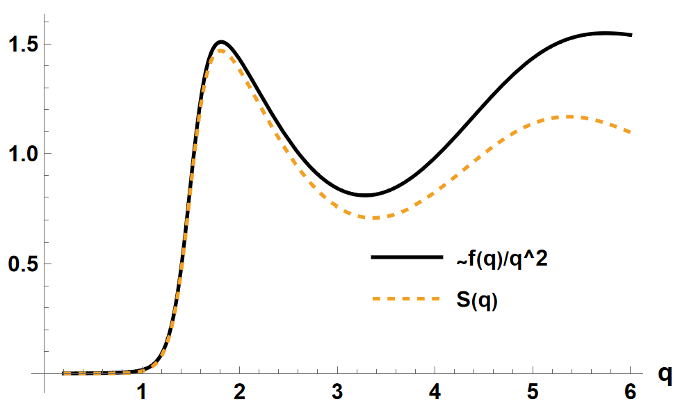
What remains to be understood is how to incorporate, within this theoretical framework, the empirical observation that the flat-band intensity closely follows the static structure factor $S(q)$, namely the condition labelled as (iii) in the above list. In this respect, it is important to note that the flat-band intensity is directly proportional to the resonant coupling $g(q)$. Therefore, if this correlation is robust and universal, it suggests that the coupling $g(q)$ itself must scale proportionally with $S(q)$.

In general, the intensity of the flat band defined as $S(q,\omega_{\mathrm{QLV}})\equiv f(q)$ is given by:

$$f(q)=\frac{\xi\,q^{2}\left[g(q)+\gamma\omega_{\mathrm{QLV}}^{2}\Gamma(q)\right]}{\left[\left(g(q)+\gamma\omega_{\mathrm{QLV}}^{2}\Gamma(q)\right)^{2}+\gamma^{2}\omega_{\mathrm{QLV}}^{2}\left(\omega_{\mathrm{QLV}}^{2}-\Omega(q)^{2}\right)^{2}\right]}.$$

(11)

with

$$\xi=\frac{2k_{B}T\gamma}{M\pi}.$$

(12)

We now discuss the general conditions under which the full expression $f(q)$ is proportional to $g(q)$ up to a power of $q$, without specifying the functional form of $\Omega(q)$ and $\Gamma(q)$. A scaling of the form $f(q)\propto q^{m}g(q)$ (with $m=2$ in the present case due to the explicit prefactor) is obtained provided two main conditions are satisfied. First, the numerator must be dominated by $g(q)$, which requires

$$g(q)\gg\gamma\omega_{\mathrm{QLV}}^{2}\Gamma(q).$$

(13)

Second, the denominator must be effectively independent of the detailed $q$-dependence of $g(q)$, which is achieved when the term proportional to $(\omega_{QLV}^{2}-\Omega(q)^{2})^{2}$ dominates. This requires

$$\left(g(q)+\gamma\omega_{\mathrm{QLV}}^{2}\Gamma(q)\right)^{2}\ll\gamma^{2}\omega_{\mathrm{QLV}}^{2}\left(\omega_{\mathrm{QLV}}^{2}-\Omega(q)^{2}\right)^{2}.$$

(14)

In addition, one must remain away from the resonance condition $\Omega(q)\approx\omega_{\mathrm{QLV}}$, where the denominator develops strong $q$-dependence and the scaling breaks down. Under these conditions, the denominator is controlled by the detuning term. If this detuning varies slowly over the $q$-range of interest compared with the oscillatory structure of $g(q)$, then the dominant modulation of $f(q)/q^{2}$ follows $g(q)$, namely

$$f(q)\propto q^{2}g(q).$$

(15)

Deviations from this behavior arise when the dissipative contribution $\Gamma(q)$ dominates the numerator, when the $(g(q)+\cdots)^{2}$ term controls the denominator, or in the vicinity of the resonance, where the response is no longer governed by a simple scaling form.

In the regime where Eq. (15) applies, assuming $g(q)\propto S(q)$ directly implies that the flat-band intensity $f(q)$ strongly correlates with the static structure factor, consistent with simulation and experimental results Li et al. (2025); Mahajan et al. (2026). We note that, since $S(0)\neq 0$, the proportionality discussed above must include an overall factor that vanishes in the $q\to 0$ limit in order to ensure that $g(0)\to 0$. A natural candidate is a power-law prefactor of the form $\sim q^{n}$.

In Fig. 4, we present an example in which these constraints are satisfied, demonstrating that the intensity of the flat band closely follows the trend of the static structure factor, as encoded in the coupling $g(q)\propto S(q)$. This analysis shows that the model naturally captures the observed strong correlation between the flat-band intensity and the static structure factor $S(q)$ Li et al. (2025); Mahajan et al. (2026), provided that the coupling $g(q)$ is taken to be proportional to $S(q)$. The physical interpretation of this choice warrants further investigation and will be briefly discussed in the following sections.

It is worth noting that, within this model, the correlation with the static structure factor is not limited to the intensity of the flat band, but also extends to its frequency. In particular, the position of the flat band—identified as the non-phononic peak in the dynamic structure factor—is not strictly $q$-independent and equal to $\omega_{\mathrm{QLV}}$. Instead, it exhibits a clear $q$-modulation, primarily governed by the form of the resonant coupling $g(q)$, which, as discussed above, is proportional to $S(q)$.

In the top panel of Fig. 5, we present an illustrative example in which this feature is intentionally enhanced by isolating the flat-band signal and shifting the phonon dispersion to higher frequencies. There, we can observe a pronounced anti-correlation between $g(q)\propto S(q)$ (black dashed line) and the flat-band frequency (white signal or blue filled line). When the resonant coupling is large, the flat-band frequency is reduced, following the oscillatory behavior of $S(q)$. In contrast, at large wave vectors—where $S(q)$, and thus $g(q)$, lose their oscillatory character—the flat-band frequency becomes nearly $q$-independent and approaches $\omega_{QLV}$. This is consistent with the fact that, in the large-$q$ limit, the static structure factor approaches unity while its oscillations become progressively damped. As a result, the oscillatory features observed in both the intensity and the frequency of the flat band gradually average out at large $q$.

Interestingly, the trend of the flat-band frequency derived from the resonant-coupling model is consistent with simulation results (see bottom panel of Fig. 5) and provides a potential direct test of the theoretical scenario proposed here.

After discussing in detail several key features of the model, and showing its ability to reproduce the main features observed in experiments and simulations, we now turn to a concrete example illustrating the evolution of the two-peak structure as the wavevector $q$ increases. While this behavior can be tracked analytically due to the simplicity of the model, for clarity of presentation we instead focus on an explicit example in which the trend closely resembles the simulation results shown in Fig. 1.

The results are presented in Fig. 6. At low $q$, the response is dominated by the acoustic phonon peak, while the non-phononic contribution is suppressed, as the coupling $g(q)$ is approximately vanishing for $q\lesssim 2$ in this example (see inset in top-left panel). As the wavevector $q$ increases, the intensity of the non-phononic flat-band signal grows, while that of the acoustic phonon decreases. At the same time, the acoustic phonon peak broadens, since its damping increases with $q$. For sufficiently large $q$, the non-phononic contribution becomes dominant, and its position remains approximately independent of $q$, i.e., it is flat. Upon further increasing the wavevector (not shown in Fig. 6), the phononic contribution becomes essentially negligible, leaving a pronounced flat-band signal at approximately $\omega\approx\omega_{\mathrm{QLV}}$ whose intensity is mainly governed by the behavior of the resonant coupling $g(q)$. Overall, these features are in good qualitative agreement with the simulation results shown in Fig. 1, as well as with other observations reported in the literature discussed above.

After analyzing the main features of the dynamical structure factor $S(q,\omega)$ and the emergence of the non-phononic flat-band signal, we now turn to the discussion of the corresponding vibrational density of states (VDOS).

The VDOS $D(\omega)$ can be directly derived from the Green’s function in Eq. (1),

$$D(\omega)=-\frac{2\omega}{\pi}\sum_{\alpha}\int\frac{d^{d}q}{(2\pi)^{d}}\,\imaginary G_{\alpha}(q,\omega).$$

(16)

where $d$ is the spatial dimension of the system.

For simplicity, in the rest of this discussion we will drop the polarization label $\alpha$ and consider a single branch.

In Fig. 7, we present a benchmark example illustrating the emergence of a boson-peak (BP) anomaly in the three-dimensional Debye-reduced density of states, $D(\omega)/\omega^{2}$. The BP position matches closely the bare frequency of the flat band in the model, $\omega_{\mathrm{QLV}}$, with a slight downward shift due to damping-induced softening and hybridization effects. This observation imposes a further constraint on the RCM, that is that the QLV frequency $\omega_{\mathrm{QLV}}$ entering in Eq. (1) has to match the BP frequency observed in the reduced VDOS.

We notice that, within the approximation used to define the resonant wave vector in Eq. (8), the identification $\omega_{\mathrm{QLV}}=\omega_{\mathrm{BP}}$ implies $q^{\mathrm{res}}=\omega_{\mathrm{BP}}/v$. Using simulation data for several amorphous systems reported in Ref. Mahajan et al. (2026) (see bottom panel in Fig. 5 for the case of the 3D CuZr metallic glass), we verified that $\omega_{\mathrm{BP}}/v$ is systematically smaller than the position of the first diffraction peak, $q^{*}$, in the static structure factor $S(q)$. Within the theoretical framework developed here, this observation is consistent with the absence of an avoided crossing in the spectrum and therefore provides additional support for the validity of our interpretation.

At the same time, this minimal model makes it clear that the boson peak is not simply the result of a broadened Van Hove singularity, as sometimes suggested (see, e.g., Chumakov et al. (2011)). This is consistent with simulations and experimental results proving the independence of these two features, e.g., Wang et al. (2018). Whether a well-defined Van Hove feature coexists with a genuine boson peak depends primarily on the strength of phonon damping and on the separation of scales between $\omega_{\mathrm{QLV}}$ and $\omega_{\mathrm{VH}}$. In particular, sufficiently strong damping $\Gamma(q)$ broadens the Van Hove singularity to the point that it is no longer distinguishable. For example, in the case considered in Fig. 7, the phonon damping is chosen to be very small, such that the phonon dispersion retains a large intensity up to very large values of $q$, thereby producing a strong and well-defined Van Hove peak in the corresponding VDOS.

Within this resonant-coupling framework the boson-peak frequency is then primarily set by the flat-band frequency in the dynamical structure factor. This behavior is consistent with observations from both simulations and experiments Hu and Tanaka (2022); Mizuno and Minamitani (2026); Mizuno et al. (2025); Mahajan et al. (2026), and indicates that the flat band plays a central role in the origin of the boson peak in amorphous solids. More broadly, these results support the view that the boson peak is largely of non-phononic origin, emerging from the resonant coupling between non-phononic modes—modeled here as quasi-localized vibrations (QLVs)—and acoustic phonons.

In general, we expect the boson peak to also receive contributions from the phononic sector. Whether these contributions are always subleading compared to those arising from the flat band remains an open question. Within our model, the answer depends sensitively on several factors, including the $q$-range over which the flat band exists and its damping. A more direct comparison with numerical simulation models is therefore needed to clarify this issue. Nevertheless, we mention that recent simulation results Mizuno and Minamitani (2026) support the idea that the boson-peak signal is dominated by the flat-band contribution.

References

- Chaikin and Lubensky (1995) P. M. Chaikin and T. C. Lubensky, Principles of condensed matter physics, Vol. 10 (Cambridge university press Cambridge, 1995).
- Ramos (2022) M. Ramos, Low-temperature Thermal And Vibrational Properties Of Disordered Solids: A Half-century Of Universal ”Anomalies” Of Glasses (World Scientific Publishing Company, 2022).
- Phillips (1981) W. Phillips, Amorphous Solids: Low-temperature Properties, Topics in current physics (Springer-Verlag, 1981).
- Pohl et al. (2002) R. O. Pohl, X. Liu, and E. Thompson, Rev. Mod. Phys. 74, 991 (2002).
- Esquinazi (1998) P. Esquinazi, ed., Tunneling Systems in Amorphous and Crystalline Solids (Springer-Verlag, Berlin, Heidelberg, 1998).
- Flubacher et al. (1959) P. Flubacher, A. Leadbetter, J. Morrison, and B. Stoicheff, Journal of Physics and Chemistry of Solids 12, 53 (1959).
- Nakayama (2002) T. Nakayama, Reports on Progress in Physics 65, 1195 (2002).
- Hu and Tanaka (2022) Y.-C. Hu and H. Tanaka, Nature Physics 18, 669 (2022).
- Hu and Tanaka (2023) Y.-C. Hu and H. Tanaka, Physical Review Research 5, 023055 (2023).
- Mahajan et al. (2026) S. Mahajan, L.-Z. Huang, C. Jiang, Y.-J. Wang, M. P. Ciamarra, J. Zhang, and M. Baggioli, “A flat-band perspective on the boson peak in amorphous solids,” (2026), arXiv:2509.06340 [cond-mat.soft] .
- Li et al. (2025) X. Y. Li, H. P. Zhang, S. Lan, D. L. Abernathy, C. H. Hu, L. R. Fan, M. Z. Li, and X.-L. Wang, Nature Communications 17, 860 (2025).
- Mizuno et al. (2025) H. Mizuno, T. Mori, G. Baldi, and E. Minamitani, “Boson peak in covalent network glasses: Isostaticity and marginal stability,” (2025), arXiv:2508.20481 [cond-mat.dis-nn] .
- Mizuno and Minamitani (2026) H. Mizuno and E. Minamitani, “Boson peak in the dynamical structure factor of network- and packing-type glasses,” (2026), arXiv:2601.19118 [cond-mat.soft] .
- Jiang et al. (2024a) C. Jiang, Z. Zheng, Y. Chen, M. Baggioli, and J. Zhang, Phys. Rev. Lett. 133, 188302 (2024a).
- Baldi et al. (2008) G. Baldi, V. M. Giordano, G. Monaco, F. Sette, E. Fabiani, A. Fontana, and G. Ruocco, Phys. Rev. B 77, 214309 (2008).
- Ruzicka et al. (2004) B. Ruzicka, T. Scopigno, S. Caponi, A. Fontana, O. Pilla, P. Giura, G. Monaco, E. Pontecorvo, G. Ruocco, and F. Sette, Phys. Rev. B 69, 100201 (2004).
- Baldi et al. (2022) G. Baldi, A. Fontana, and G. Monaco, in Low-Temperature Thermal and Vibrational Properties of Disordered Solids: A Half-Century of Universal “Anomalies” of Glasses, edited by M. A. Ramos (World Scientific, 2022) pp. 177–226.
- Tømterud et al. (2023) M. Tømterud, S. D. Eder, C. Büchner, L. Wondraczek, I. Simonsen, W. Schirmacher, J. R. Manson, and B. Holst, Nature Physics 19, 1910 (2023).
- Steurer et al. (2007) W. Steurer, A. Apfolter, M. Koch, W. E. Ernst, B. Holst, E. Søndergård, and J. R. Manson, Phys. Rev. Lett. 99, 035503 (2007).
- Tømterud et al. (2025) M. Tømterud, S. D. Eder, S. K. Hellner, C. Büchner, M. Heyde, H.-J. Freund, S. Forti, D. Convertino, C. Coletti, J. R. Manson, and B. Holst, Phys. Rev. B 111, 205423 (2025).
- Meyer et al. (1996) A. Meyer, J. Wuttke, W. Petry, A. Peker, R. Bormann, G. Coddens, L. Kranich, O. G. Randl, and H. Schober, Phys. Rev. B 53, 12107 (1996).
- Inoue et al. (1991) K. Inoue, T. Kanaya, S. Ikeda, K. Kaji, K. Shibata, M. Misawa, and Y. Kiyanagi, The Journal of chemical physics 95, 5332 (1991).
- Rufflé et al. (2006) B. Rufflé, G. Guimbretière, E. Courtens, R. Vacher, and G. Monaco, Phys. Rev. Lett. 96, 045502 (2006).
- (24) H. Mizuno and A. Ikeda, “Computational simulations of the vibrational properties of glasses,” in Low-Temperature Thermal and Vibrational Properties of Disordered Solids, Chap. Chapter 10, pp. 375–433.
- Buchenau (1992) U. Buchenau, Philosophical Magazine B 65, 303 (1992).
- Laird and Schober (1991) B. B. Laird and H. R. Schober, Phys. Rev. Lett. 66, 636 (1991).
- Schober and Laird (1991) H. R. Schober and B. B. Laird, Phys. Rev. B 44, 6746 (1991).
- Buchenau et al. (1996) U. Buchenau, A. Wischnewski, D. Richter, and B. Frick, Phys. Rev. Lett. 77, 4035 (1996).
- Buchenau et al. (1988) U. Buchenau, H. M. Zhou, N. Nucker, K. S. Gilroy, and W. A. Phillips, Phys. Rev. Lett. 60, 1318 (1988).
- Karpov et al. (1983) V. G. Karpov, M. I. Klinger, and F. N. Ignat’ev, Soviet Physics JETP 57, 439 (1983), russian original: Zh. Eksp. Teor. Fiz. 84, 760–775 (1983).
- Karpov and Parshin (1985) V. G. Karpov and D. A. Parshin, Soviet Physics JETP 61, 1308 (1985), russian original: Zh. Eksp. Teor. Fiz. 88, 2212–2227 (1985).
- Buchenau et al. (1991) U. Buchenau, Y. M. Galperin, V. L. Gurevich, and H. R. Schober, Phys. Rev. B 43, 5039 (1991).
- Gurevich et al. (2003a) V. L. Gurevich, D. A. Parshin, and H. R. Schober, Phys. Rev. B 67, 094203 (2003a).
- Parshin et al. (2007) D. A. Parshin, H. R. Schober, and V. L. Gurevich, Phys. Rev. B 76, 064206 (2007).
- Buchenau et al. (1992) U. Buchenau, Y. M. Galperin, V. L. Gurevich, D. A. Parshin, M. A. Ramos, and H. R. Schober, Phys. Rev. B 46, 2798 (1992).
- Schober and Oligschleger (1996) H. R. Schober and C. Oligschleger, Phys. Rev. B 53, 11469 (1996).
- Schober et al. (1993) H. Schober, C. Oligschleger, and B. Laird, Journal of Non-Crystalline Solids 156-158, 965 (1993).
- Luchnikov et al. (2000) V. A. Luchnikov, N. N. Medvedev, Y. I. Naberukhin, and H. R. Schober, Phys. Rev. B 62, 3181 (2000).
- Schober (2004) H. R. Schober, Journal of Physics: Condensed Matter 16, S2659 (2004).
- Schober (2011) H. Schober, Journal of Non-Crystalline Solids 357, 501–505 (2011).
- Lerner and Bouchbinder (2021) E. Lerner and E. Bouchbinder, The Journal of Chemical Physics 155, 200901 (2021).
- Lerner and Bouchbinder (2023) E. Lerner and E. Bouchbinder, The Journal of Chemical Physics 158, 194503 (2023).
- Moriel et al. (2024a) A. Moriel, E. Lerner, and E. Bouchbinder, Phys. Rev. Res. 6, 023053 (2024a).
- Moriel et al. (2024b) A. Moriel, E. Lerner, and E. Bouchbinder, Journal of Applied Physics 136, 225105 (2024b).
- Mahajan and Ciamarra (2021) S. Mahajan and M. P. Ciamarra, Phys. Rev. Lett. 127, 215504 (2021).
- Mahajan et al. (2025) S. Mahajan, D. Seow Yang Han, C. Jiang, M. Baggioli, and M. P. Ciamarra, Phys. Rev. E 112, 035413 (2025).
- Mahajan and Ciamarra (2023) S. Mahajan and M. P. Ciamarra, SciPost Phys. 15, 069 (2023).
- Flenner and Szamel (2025a) E. Flenner and G. Szamel, Science Advances 11, eadu6097 (2025a).
- Flenner and Szamel (2025b) E. Flenner and G. Szamel, The Journal of Physical Chemistry B 129, 1855 (2025b).
- Zhang et al. (2021) H. Zhang, X. Wang, H.-B. Yu, and J. F. Douglas, The Journal of Chemical Physics 154, 084505 (2021).
- Jiang et al. (2024b) C. Jiang, M. Baggioli, and J. F. Douglas, The Journal of Chemical Physics 160, 214505 (2024b).
- Jiang and Baggioli (2024) C. Jiang and M. Baggioli, Journal of Physics: Condensed Matter 36, 505101 (2024).
- Bianchi et al. (2020) E. Bianchi, V. M. Giordano, and F. Lund, Phys. Rev. B 101, 174311 (2020).
- Lund and Scheihing-Hitschfeld (2026) F. Lund and B. Scheihing-Hitschfeld, “Quantum theory of elastic strings and the thermal conductivity of glasses,” (2026), arXiv:2601.12721 [cond-mat.mtrl-sci] .
- Pang (1992) T. Pang, Phys. Rev. B 45, 2490 (1992).
- Malinovsky et al. (1991) V. Malinovsky, V. Novikov, and A. Sokolov, Physics Letters A 153, 63 (1991).
- Maurer and Schirmacher (2004) E. Maurer and W. Schirmacher, Journal of Low Temperature Physics 137, 453 (2004).
- Maradudin et al. (1971) A. A. Maradudin, E. W. Montroll, G. H. Weiss, and I. P. Ipatova, Theory of Lattice Dynamics in the Harmonic Approximation, 2nd ed., Solid State Physics Supplement, Vol. 3 (Academic Press, New York, 1971).
- Gurevich et al. (2003b) V. L. Gurevich, D. A. Parshin, and H. R. Schober, Phys. Rev. B 67, 094203 (2003b).
- Fetter and Walecka (1971) A. L. Fetter and J. D. Walecka, Quantum Theory of Many-Particle Systems (McGraw-Hill, New York, 1971).
- Akhiezer (1939) A. I. Akhiezer, Journal of Physics (USSR) 1, 277 (1939).
- Klemens (1955) P. G. Klemens, Proceedings of the Physical Society. Section A 68, 1113 (1955).
- Wang et al. (2020) L. Wang, G. Szamel, and E. Flenner, Soft Matter 16, 7165 (2020).
- Chumakov et al. (2011) A. I. Chumakov, G. Monaco, A. Monaco, W. A. Crichton, A. Bosak, R. Rüffer, A. Meyer, F. Kargl, L. Comez, D. Fioretto, H. Giefers, S. Roitsch, G. Wortmann, M. H. Manghnani, A. Hushur, Q. Williams, J. Balogh, K. Parliński, P. Jochym, and P. Piekarz, Phys. Rev. Lett. 106, 225501 (2011).
- Wang et al. (2018) Y. Wang, L. Hong, Y. Wang, W. Schirmacher, and J. Zhang, Phys. Rev. B 98, 174207 (2018).
- Tian et al. (2021) Y. Tian, X. Shen, Q. Gao, Z. Lu, J. Yang, Q. Zheng, C. F. Aleman, D. Luo, A. H. Reid, B. Xu, et al., arXiv preprint arXiv:2111.10171 (2021).
- Qi et al. (2026) Y. Qi, N. Chen, Z. Zhou, Q. Xu, Y. Lv, X. Zou, T. Jiang, P. Zhu, M. Zhu, D. Chen, Z. Sun, X. Li, and D. Xiang, “Direct observation of ultrafast amorphous-amorphous transitions indicated by bond stretching and angle bending in phase-change material gete,” (2026), arXiv:2603.17400 [cond-mat.mtrl-sci] .
- Schirmacher and Ruocco (2022) W. Schirmacher and G. Ruocco, “Heterogeneous elasticity: The tale of the boson peak,” in Low-Temperature Thermal and Vibrational Properties of Disordered Solids (World Scientific, 2022) Chap. 9, pp. 331–373.
- Ding et al. (2025) G. Ding, E. Ma, F. Jiang, J. Duan, S. Cai, N. Xu, B. Cui, L. Dai, and M. Jiang, Nature Physics 21, 1911 (2025).