Recently, quantum corrections of black hole radiation for various situations, solution and quantities have been calculated, see [Iliesiu:2020qvm, Heydeman:2020hhw, Iliesiu:2022onk, Kapec:2023ruw, Maulik:2024dwq, Nian:2025oei, PandoZayas:2025snm, Maulik:2025hax], among other works. These quantum corrections become important specially at low-temperature and dominate the dynamics of the black hole.

In [Brown:2024ajk], it has been demonstrated that these quantum effects at low-temperature and in microcanonical ensemble would actually slow down the emission of quantum radiation near the horizon of the black hole, by a factor of $10^{700}$. There, it has been shown that the black hole alternates between exponentially long epochs of integer and half-integer spin which have very different cooling rates. Here, in our first section, we argue that if we actually consider near the black hole region as an open quantum system, passing through the exceptional points (EPs) would actually cause the same effect, similar to the roles of EPs in the dynamics of SYK model as discussed in [Zheng:2025apa].

In the canonical ensemble, [Brown:2024ajk] shows that the energy flux in the exact quantum-corrected solution would be larger than the semiclassical flux at fixed temperature $T$. This is in contradiction with the microcanonical result, where it would be a reduced flux relative to the semiclassical case at very low energies. So, in the canonical ensemble, the increase in typical energy leads to an increase in the expected flux relative to the semiclassical prediction. The resolution is that the relation $M-Q=\frac{2\pi^{2}}{E_{\text{brk}}}T^{2}$ would break at low temperatures. This also can be explained by considering the presence of EPs near the black hole horizon, as we show in our first section here.

Previously, in the semiclassical regime, the greybody factor and Hawking radiation have been calculated in [Cvetic:1997uw, Lee:1998pd, Setare:2006hq, Jiang:2007pn, Cvetic:2009jn]. Recently, quantum corrections to these quantities, and many other thermodynamical quantities have also been calculated, mainly based on the new methods of [Brown:2024ajk].

In addition, in various recent works, the effects of quantum fluctuations at low temperature near extremal and near horizon geometries have been examined using the one dimensional Shwarzian effective action. Note that the Schwarzian modes are the zero modes in JT. One could then consider these fluctuations more precisely and go to one dimension higher and instead of near $\text{AdS}_{2}$ geometry, consider the full $\text{AdS}_{3}$ case or its reparameterized version [Cotler:2018zff], which is the main goal of this work.

In [Cotler:2018zff], the $\text{PSL}(2;\mathbb{R})$-invariant bilocal operators have been studied extensively, and the authors showed that the connected two-point function of bilocals is the Virasoro identity block. Then, they argued for the gravity dual of a bilocal probe. They noted that, as bilocal operators in the Schwarzian theory and in nearly-$\text{AdS}_{2}$ gravity correspond to boundary insertions of sources for operators dual to bulk matter field, the extended picture in $3d$ could be envisioned for the reparametrized $\text{AdS}_{3}$ case of [Cotler:2018zff] as well. The probe in this case would be dual to a bulk Wilson like which ends on the AdS boundary at the two points of the bilocal. This picture could help us to understand Schwarzian quantum corrections to various parameters of the black hole from one dimension higher point of view of the nearly $\text{AdS}_{2}$ case. We also use, the results of [Fitzpatrick:2016mtp, Blommaert:2018oro], along the way.

So the plan of this work is as follows. First, in section 2, we study black holes in the Lindblad formalism and as an open quantum system. We compare each quantity, such as Green’s function, action, transition amplitude, bilocal operators and couplings, for the open quantum system and the theory of AdS₃ with reparametrization modes, as discussed in Cotler and Jensen work [Cotler:2018zff]. Then, in section 3, we study the theory of reparamtrized AdS₃ further. We compare the structure of this theory with JT, and find the quantum corrected free propagator and actions. Then, we find the one-loop corrected greybody factor for this theory, along with other black hole solution in section 4. We also find the quantum corrected Lyapunov exponent in section 5. Next, we discuss quantum corrections to some other black hole quantities such as potential, and information structures such as information inequalities in section 6. We conclude with a brief discussion in section 7.

In [PandoZayas:2025snm], the authors studied the effects of quantum fluctuations for near-extremal asymptotically $\text{AdS}_{4}$ black branes, where they found that at one-loop level, there is a coupling between the shear gravitational fluctuations to “one of the would-be zero modes”, and this coupling would affect the retarded Green’s function which leads to low temperature violation of the shear viscosity to entropy density bound. On the other hand, in [Zheng:2025apa], the dynamics of Lindblad SYK model coupled to a bath has also been studied, where the authors found a nontrivial, non-monotonic feature, which is due to the presence of exceptional points and its proliferation. This non-monotonic behavior is actually in the behavior of dissipative gap versus the bath coupling $\mu$ of the system. Here, we aim to connect these two works and these two effects, and therefore explain the observed zig-zag behavior in the Page-cure of radiation with quantum corrections.

Note that in the extremal limit of black holes, and in its throat region, one has an effective theory which contains the Schwarzian geometry. One could imagine the quantum correction of this geometry as an open quantum system which contains a system coupled to a bath, and then apply the results and methods of [Zheng:2025apa], such as the vectorization of density matrix, and also apply the Lindblad formalism.

The gravitational path integral over the zero modes in this system, would affect the Green’s function which were studied in [PandoZayas:2025snm]. On the other hand, the connections between Green’s function, partition function and dissipative gap were studied in [Zheng:2025apa].

For the SYK model, which has strong connection to Schwarzian model, the on-shell Green’s function $G_{ab}$ in the large-N limit would be

where $a,b\in\{+,-\}$.

In the action, in addition to Green’s function, one should consider another bilocal field $\sigma_{ab}$ as well, which for the case of Lindblad SYK leads to [Zheng:2025apa]

For the case of black hole, the Green’s function has the form of [PandoZayas:2025snm]

Then, the tree-level Green’s function would be

The one-loop Green’s function here is

One should then be able to define a coupling between these two sectors and show its non-monotonic behavior as in [Zheng:2025apa].

Now, one could imagine similar effects due to the presence of exceptional points in the Schwarzian modes of quantum fluctuations around the horizon of black holes. In addition, the behavior of such exceptional points from one dimension higher point of view could also be studied later.

The one-loop corrections can be considered by taking into account the gravitational fluctuations to quadratic order, as [PandoZayas:2025snm]

So, as discussed in [PandoZayas:2025snm], the bulk field $\phi$ couples to $h_{\text{zero}}$ via its action $h_{\text{zero}}\Delta_{L}h_{\text{zero}}$. The bulk field $\phi$ then could be considered as bath, and $h_{\text{zero}}$ with the action $h_{\text{zero}}\Delta_{L}h_{\text{zero}}$ as the system. If one takes $\mu$ as the coupling between them, one could see a non-monotonic behavior similar to the case of [Zheng:2025apa].

The Lichnerowicz operator here is

where $\Delta_{EH}^{\alpha\beta,\mu\nu}$, $\Delta_{1}^{\alpha,\beta,\mu\nu}$, $\Delta_{F}^{\alpha\beta,\mu\nu}$ are the contribution from the Einstein-Hilbert, cosmological constant and the Maxwell action respectively. The change of saddle and the non-monotonic behavior of quantities such as dissipative gap $\Gamma_{0}$ versus bath coupling $\mu$ can be explained by the change in the contribution from each term. So, considering the sum of these operators as a matrix, the exponential points here could be detected by finding where the eigenvalue and eigenstates coalesces. Note that, the theory of low energy Schwarzian modes [Daguerre:2023cyx, Liu:2024gxr, Jensen:2016pah] is similar to SKY and Lindblad SYK model of [Zheng:2025apa].

In [PandoZayas:2025snm], the one-loop correction for the case of $n\geq 2$ has been calculated as

where $\alpha=\frac{2\pi l^{2}}{r_{0}}$.

The field $\delta g$ couples with the zero modes through the “lifted eigenvalue” $\delta\Lambda_{n}[\delta g]$ in the near-horizon “throat”.

Also, one would expect that the dissipative gap $\Gamma_{0}$ versus the coupling between the shear gravitational fluctuations to the zero mode would be non-monotonic, similar to the case of [Zheng:2025apa]. As times progress, this coupling changes and as the result, the dissipative gap changes, which affects all the thermodynamical quantities of the black holes and the quantum corrections effects, such as the ratio of shear viscosity to entropy density.

At zero temperature, where $g=g^{(0)}$ and $A=A^{(0)}$, the form of zero modes would be

Note that the zero modes and Schwarzian modes are related with each other as discussed in [Iliesiu:2022onk].

One would then expect in the black hole systems, the decay rate toward steady states would be a non-monotonic function of the bath coupling $\mu$ similar to the case of [Zheng:2025apa, Jensen:2016pah].

The quantum corrected “cloud” around the naked quantity could be considered as the bath. If one turns on a small temperature, the lifted eigenvalues would be

One then could consider the term $h_{\alpha\beta}^{(n)*}\delta\Delta_{L}^{\alpha\beta,\mu\nu}h_{\mu\nu}^{(n)}$.

So, if we consider SYK or Schwarzian and double the Hilbert state, we could get the following relationship

In the setup with quantum corrections, for a bosonic system, the transition amplitude would have the following path integral representation

So the coupling between the system and the bath, (or the correlations between the bare system and the quantum corrected one) can move the system forward, leading to the following relation

Then, one could propose the following relation between Lindblad SYK and Swarzian mode of quantum corrections

where $t_{++}=t_{--}=1$, $t_{+-}=t_{-+}=-(-1)^{q/2}$, $a,b\in\{+,-\}$, and in the large $N$, one has

Here $G_{ab}$ and $\sigma_{ab}$ are the Green’s function and self-energy respectively, which by the above relation could be connected to the conjugate momentum $\pi(\mathbf{x})$.

Note that by a vectorization procedure, the Hilbert space would be doubled, where the Lagrangian becomes [Kulkarni_2022]

Therefore, one could imagine the quantum correction around the JT in the near horizon of black hole as a Markovian reservoir coupled to an SYK model, and the jump operator which are related to Hawking radiation, would be either linear or quadratic in the Majorana fermion operators. The distribution of linear jump operator or quadratic jump operators could be Gaussian, linear, or other statistical functions which needs to be specified for each case.

The Hawking particle creation could then be modeled by a linear jump operator $L^{i}=\sqrt{\mu}\psi^{i},i=1,...,N$, or by quadratic jump operators $L^{a}=\sum_{1\leq i<j\leq N}K_{ij}^{a}\psi_{i}\psi_{j}$, which would be related to one-loop or two loops quantum corrections.

Here, we could also write the fields as

In the large-q limit, the expansion of the Green’s function would be

where $q$ is the q-body interaction in SYK model, which is related to Newton constant $g$, as

The bilocal operator here is

The coupling of the above operator to the reparametrization field $\phi=\alpha_{0}\theta+\frac{\epsilon}{\sqrt{C}}$ can be found as [Cotler:2018zff, Fitzpatrick:2015foa, Chen:2017dnl]

So, we expect that $q$ is related to $\frac{\sqrt{C}}{h}$ or to $g^{2}$. In fact, this picture that we construct here, is also related to the explicit exchange of Virasoro gravitons between heavy and light $\text{CFT}_{2}$ operators at large central charge, as explained in [Fitzpatrick:2015foa, Fitzpatrick:2016mjq].

The heavy-light OPE Virasoro blocks, and their connections to thermodynamics of black holes have also been studied in [Fitzpatrick:2014vua, Fitzpatrick:2015zha]. Note that unlike the study of [Qi:2019gny] which used the Feynman diagrams, in these works, the authors used the on-shell method which is simpler for various examples.

The Catalan number $C_{k}$, then, is related to the number of distinct three diagrams with $k$ vertices which is related to the size of the bare system. Note that the bare system here is the BTZ black hole with Hawking temperature $T_{H}$ and with no quantum corrections.

The mode expansion of holomorphic stress tensor can then be written as

where these $L$-generators act on the vacuum and create non-trivial states, and they are related to the linear jump operators in the Lindblad formalism.

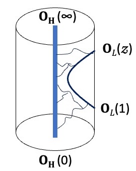
The exchange of graviton states between a heavy object (which is considered as the system here) and the light probe (which is considered as the bath in initial stages), could be written as

So the coupling between the two would be

The matrix $\mathcal{N}_{\{b_{l}\},\{a_{k}\}}$ would vanish here unless $a_{i}=b_{j}$, and so we have

The behavior of $\mathcal{V}(z)$ versus $h_{H}$ is shown in Figure 1, and the schematic behavior of this exchange of gravitons and the double-trace operators between heavy and light operators near the horizon of black holes is shown in Figure 2.

The dissipative gap versus this coupling would have a non-monotonic behavior as in [Zheng:2025apa], which is related to the non-monotonicity of $\mathcal{V}(z)$.

So, one would also expect that the generating function of the Catalan number at $\frac{6h_{H}}{c}$ which builds the temperature of a BTZ black hole, is related to the size of SKY model $N$ as in

where for the case of thermofield double state (TFD), one can write

With the Hamiltonian $H_{\text{tot}}=H_{L}+H_{R}$, the time evolution would be $U(t)=e^{-iH_{\text{tot}}t}$, and the fermionic bilinear coupling would be

Note that an operator like $\langle\mathcal{O}_{H}(\infty)\mathcal{O}_{H}(1)\left(\sum_{\psi}\ket{\psi}\bra{\psi}\right)\mathcal{O}_{L}(z)\mathcal{O}_{L}(0)\rangle$ could also be written as partial wave decomposition which has all the dynamical data that we need to track the black hole and its quantum corrections. The interesting point is that, in the case of AdS, the vacuum would dynamically break the Virasoro symmetry, the stress energy tensor $T(z)$, and its derivatives, similar to the jump operators in Lindblad formalism.

In [Fitzpatrick:2015foa], it has been shown that the operators of the order $\frac{1}{\sqrt{c}^{|k-l|}}$ contribute in the heavy-light limit, and as this factor $|k-l|$ changes over the evolution of black hole radiation, the non-monotonic behaviors could be expected.

Also, in [Fitzpatrick:2015zha], using other methods, the heavy-light limit of vacuum Virasoro conformal block is found as

Here $f$ is a function that will be shown only in the terms that are in single power of $h_{L}$, which would be also the case for the functionality of coupling $\mu$ between a SYK system coupled to a bath.

Note that these $a_{i}$s which are depicted in Figure 3 can be considered as momenta flow between propagators. After taking the product of the propagators, based on [Fitzpatrick:2015foa], one should multiply the result by a factor of $2.\frac{6^{k}z^{s}}{s(s-1)}$, where $s\equiv\sum_{i}a_{i}$, and as one could see from Figure 4, this factor produce non-monotonicity in the correlation.

One then can consider the action in [Fitzpatrick:2015foa] as

with the coupling $g\propto\frac{1}{\sqrt{c}}$, and note that the field $\phi(t,\theta)$ has a mode expansion in the form of

and with the propagator in the form of $\frac{i}{\omega-(m+1)}$.

Then, we could compare this mode expansion with the Loschmidt echo for dissipative quantum systems describing the overlap between initial and time evolved states of the vectorized density matrix as

So, this Loschmidt echo, can be considered as the relationship between two mode expansions, and as mode overlap.

Here, we would like to consider the effects of quantum corrections, in $3d$ and mainly in Cotler-Jensen theory of [Cotler:2018zff], which is a theory of reparameterizations for AdS₃ gravity. First, we review some aspect of this theory and explain which parts of their methods and considerations are related to our studies of quantum corrections.

As mentioned in [Cotler:2018zff], sometimes the dual of $\text{AdS}_{3}$ would be a boundary Liouville theory [Coussaert:1995zp]. We would like to know, how this boundary Liouville theory could have an effect on the greybody factor and on Hawking radiation. The pure gravity in this case is on a Lorentzian cylinder. However, one should note that in the Liouville case, the spectrum is continuous and with no normalizable vacuum, while $\text{AdS}_{3}$ has discrete spectrum and normalizable vacuum. Finding how these features will play a role in our problem with quantum corrections, would be interesting.

When one writes the pure $\text{AdS}_{3}$, on a cylinder, the boundary conditions which make the bulk asymptotically $\text{AdS}_{3}$ can constraint the gauge fields, and then the chiral Wess-Zumino-Witten (WZW) model would become a constrained $SO(2,1)\times SO(2,1)$ chiral WZW on the boundary. Then, by redefinition, it can become constrained $SO(2,1)$ WZW and then can be rewritten as a Liouville theory. So when considering the quantum fluctuation effects on the Hawking radiation and greybody factor, one should consider such constraints as well.

The field theory in this case, due to the boundary condition of $\text{AdS}_{3}$, keeps the $A_{0}$ part of $A=A_{0}dt+\tilde{A_{i}}dx^{i}$ non-zero, which then makes the boundary model to get quasi-local $SO(2,1)\times SO(2,1)$ quotient.

The main boundary theory that we consider is

which is the quantum field theory of the (left-moving) boundary gravitons of pure $\text{AdS}_{3}$ gravity.

For the case of BTZ, the boundary action is

Similar to JT, the boundary description of the two-sided BTZ black hole has non-local constrains between the degrees of freedom and between the two asymptotic boundaries, and therefore has also a non-factorization property which would affect the greybody factor and Hawking radiation.

An interesting feature of this theory is that at any fixed time, $\phi$ would be an element of $\text{Diff}(\mathbb{S}^{1})/PSL(2;\mathbb{R})$. It would be interesting to check whether adding quantum corrections, which evolve during the Hawking radiation, this fact would remain true, and also to consider their effects on the fields in the bath and islands.

Another important point in the theory we consider here [Cotler:2018zff], is that the higher-order terms are expected to be computed from the higher loops in the $1/c$ expansion, and by comparing with [Chen:2016cms], the authors found that there would be non-perturbative contributions to the Virasoro blocks at large central charge, which would be suppressed as $\text{exp}(-c)$. This in fact, might be due to instanton configurations in the theory. The effects of these terms on greybody factor or Lyapanov exponent will be studied in or work here. One might think that these reparametrization fields and modes for the case of $\text{AdS}_{3}$, unlike the JT case and nearly-$\text{AdS}_{2}$ scenario, would “not” correspond to matter fields in the gravity dual, and they just act as instantons, which only shift the central charge and move along the discrete spectrum. Also, note that this theory which we considered here, similar to JT, can support wormholes and has non-factorization behavior.

Now we can study the calculations of one-loop quantum corrections and their effects on various thermodynamical properties of black hole.