Electromagnetic Digital Twin-Enabled Closed-Loop Beam Management in ISAC Systems
Abstract
Digital twin (DT) is envisioned as a key enabler of sixth-generation (6G) communication systems, evolving from offline descriptive replicas for monitoring and analysis to in-the-loop agents within digital twin networks (DTNs) that couple physical and digital worlds. Recent advances in integrated sensing and communication (ISAC)-driven electromagnetic (EM) scattering methods enable environment twinning by linking channel behaviors to EM properties of the scatterers, supporting interpretable DT states and EM-grounded optimization. However, existing studies primarily focus on DT construction and lack mechanisms for closed-loop control in wireless systems. Moreover, array-geometry mismatch can bias DT reconstruction and degrade control performance, while prior works assume known arrays. To address these gaps, we propose an EM-ISAC-based closed-loop DTN framework with a hierarchical design integrating environment twinning, prior injection, and control decision into an end-to-end loop. Leveraging ISAC measurements, the proposed framework jointly reconstructs scatterer information and array-dependent forward operator and employs a low-complexity Bayesian message-passing algorithm to perform contrast inference and array calibration. The reconstructed DT guides codebook preselection to reduce training overhead and narrow candidate beams. Subsequently, downlink beam-forming (BF) is performed based on DT-predicted channels, enabling latency-bounded closed-loop control. Simulation results demonstrate improved robustness and control performance under array mismatch.
Index Terms:
Digital twin network, integrated sensing and communication, belief propagation, beam management.I Introduction
Digital twin (DT), as a key vision for future sixth-generation (6G) communication systems, is driving the evolution toward intelligent design and optimization in wireless networks [1, 13]. Traditionally, DT provides a digital replica of the wireless environment and network dynamics, enabling interpretable channel-aware representations and informative priors for system optimization [29]. More recently, as wireless networks become reconfigurable and adaptive, DT evolves from an offline, monitoring tool into an in-the-loop entity that bridges the physical and digital worlds, enabling closed-loop decision-making. This transition leads to the concept of digital twin networks (DTNs), which aims to achieve physically–digitally consistent and scalable system optimization [2, 12].
Against this backdrop, existing DT-enabled wireless solutions can be broadly categorized as strategies that couple DT construction with closed-loop control, depending on what is twinned and how the twin is updated and exploited. Specifically, [3] constructs a network DT for reliable edge caching, where the physical network is mirrored in the digital domain via vertical and horizontal twinning to support reliability-aware decision-making. In [4], a machine-learning-based DT is developed for predictive modeling in wind turbines and integrated with a next-generation radio access network (NG-RAN)-assisted cloud platform, enabling virtual monitoring and closed-loop feedback. In [5], a large-model-based channel DT is proposed for real-world environment intelligence, where multimodal data and learned representations are used to predict channel behaviors and facilitate downstream wireless optimization. In [6], DTs of electromagnetic (EM) propagation environments are constructed for live fifth generation (5G) networks by passively acquiring multipath parameters from in-network signals and combining EM simulation to reproduce site-specific propagation effects in the electrical domain. Furthermore, in [7], an EM-scattering-based material reconstruction approach is proposed to reconstruct environmental scatterers using endogenous data from an integrated sensing and communication (ISAC) system.
Among these paradigms, the ISAC-driven EM-scattering perspective has recently attracted increasing attention for DT construction, as it provides a physics-consistent view of wireless propagation rooted in EM field interactions [11, 12, 30]. This paradigm is particularly appealing because it enables the construction of a physical DT directly from endogenous data available in communication systems, without requiring additional sensing infrastructures. In contrast, conventional approaches to physical-world twinning often rely on extra on-site sensors, such as light detection and ranging (LiDAR) and cameras, increasing deployment costs and system complexity. By linking channel behaviors to the geometry and material properties of environmental scatterers, this approach enables reconstruction of a physically interpretable environment DT state and supports EM-grounded optimization. For wireless systems, such a physics-consistent paradigm turns environment awareness into actionable priors for beam management and resource adaptation, bridging propagation modeling with communication and sensing design [21, 29]. However, most existing studies focus primarily on DT construction, including pilot design [8], channel reconstruction [9], and analysis of reconstruction ill-conditioning [10].
A key challenge in closing the loop in practice is how to translate a reconstructed, potentially imperfect DT state into reliable and latency-constrained wireless control actions. Achieving this goal requires trustworthy sensing and beam-forming (BF) models that remain robust under model mismatch and hardware imperfections [14, 15, 16]. Furthermore, most existing DT-enabled propagation studies assume perfectly known array geometry, under which the propagation channel and array geometry are fully determined once the environment DT is obtained. In realistic settings, however, the array geometry is often unknown or mismatched, which can distort both the scattering operator and the array manifold, thereby biasing the reconstructed DT and degrading the reliability of the resulting closed-loop control actions. Consequently, array calibration becomes a critical component of the overall pipeline.

Motivated by the above gaps, we develop an electromagnetic digital-twin-based closed-loop DTN framework realized through ISAC systems. Specifically, we move beyond environment twinning and focus on making the reconstructed DT actionable for latency-bounded wireless control under non-ideal hardware conditions. To this end, we explicitly account for array calibration by jointly inferring the environment state and the array-dependent forward operator, enabling reliable downstream beam management and BF decisions.
To operationalize this vision, we develop a unified inference-and-control framework that closes the loop from environment twinning to executable beam management. The proposed framework consists of two tightly coupled stages: DT reconstruction and closed-loop control. In the first stage, DT reconstruction aims to recover the physical information of the environment, such as the material properties of the scatterers and the geometry of the antenna array. To address the large problem size, we adopt Gaussian belief propagation (GaBP) [17, 18, 19] as a low-complexity Bayesian message-passing engine, with an alternating procedure that performs contrast inference and array calibration within a unified computational backbone, yielding an uncertainty-aware environment DT. In the second stage, closed-loop beam management is built upon the reconstructed DT: DT-guided codebook preselection reduces training overhead, while uncertainty-aware downlink BF based on the DT-predicted channel enables latency-bounded control with feedback. From a system-level perspective, the proposed closed-loop DTN framework trades offline DT construction and digital-domain inference for reduced over-the-air training and beam-search overhead.
The main contributions of this work are summarized as follows:
-
•
We propose a unified inference framework that jointly performs environment reconstruction and array calibration via a GaBP-driven pipeline, improving reliability for physical DT reconstruction under model mismatch.
-
•
We develop a DT-based closed-loop beam management scheme that integrates DT-guided codebook preselection with uncertainty-aware BF.
-
•
Through numerical simulations, we demonstrate that the proposed closed-loop DTN architecture can be realized entirely from endogenous communication-system data, enabling physical DT reconstruction, array calibration, and downstream beam optimization within a unified in-the-loop framework.
The remainder of this paper is organized as follows. Section II introduces the EM-ISAC system model. Section III presents the proposed GaBP-based DT reconstruction framework for scatter reconstruction and array calibration. Section IV describes the closed-loop beam management design, including DT-guided codebook preselection and uncertainty-aware BF optimization. Section V presents numerical results, and Section VI concludes the paper.
Notation: Boldface letters denote vectors and matrices. is the imaginary unit. , , and denote transpose, Hermitian transpose, and complex conjugate, respectively. , , , , and denote the real part, imaginary part, modulus, Euclidean norm, and inner product, respectively. forms a diagonal matrix from ; is the identity matrix; denotes the Khatri–Rao product; and and denote the -th row and -th column of . and denote complex Gaussian random vectors and variables, respectively, while denotes the real Gaussian distribution. , , and denote expectation, variance, and probability. denotes the generalized eigenvector associated with the largest generalized eigenvalue of . denotes the dimension of , and denotes is positive semidefinite.
II System Model
We consider a two-dimensional (2D) transverse magnetic () EM sensing scenario with an uplink multiple-input multiple-output (MIMO)-orthogonal frequency-division multiplexing (OFDM) probing protocol. The assumption is adopted for tractability, under which the EM fields are invariant along the -axis. Let denote the sensing region, which is discretized into grid points, and let denote a closed observation curve in the far field of . A co-located aperture with elements is deployed on and operates in time division duplex (TDD) mode, thus the same aperture alternates between transmission and reception. In each TDD sensing snapshot, all elements are simultaneously excited using a fully digital pilot vector, and an -dimensional baseband observation is collected during the receive phase. We assume a fully digital baseband architecture throughout.
We consider equally spaced subcarriers centered at with spacing , i.e.,
| (1) |
At subcarrier , the received baseband signal is expressed as
| (2) |
where denotes the received signal, is pilot vector, represents the end-to-end scattering channel, denotes the additive noise, is the all-zero vector, and denotes the noise variance. By reciprocity under TDD operation, the same array is used for both transmission and reception in DT construction stage.
II-A EM-Consistent Scattering Channel and Forward Operator
We adopt an EM-consistent scattering model based on the Lippmann–Schwinger equation to characterize the propagation channel, which relates the total field to the incident field and the material contrast within the sensing region. Let . Denote by and the incident and total fields at pixel , respectively. The Lippmann–Schwinger equation is given by [27]:
| (3) |
Here, is an arbitrary pixel in and denotes the complex material contrast, capturing both permittivity and conductivity variations:
| (4) |
where denotes the relative permittivity, denotes the electrical conductivity, and is the vacuum permittivity. We assume with over the probing band.
Define Green’s function as
| (5) |
where is the zeroth-order Hankel function of the second kind, , and is the speed of light.
Discretizing into yields the contrast vector and the in-domain Green’s matrix . Let denote the free-space propagation operator between the aperture points on and the grid points in . Under the co-located assumption, the transmit-to-domain and domain-to-receive operators satisfy
| (6) |
Let denote the discretized total and incident fields in , respectively. Then, the discretized Lippmann–Schwinger equation is given by
| (7) |
Rearranging yields
| (8) |
Define the induced (equivalent) scattering source in as
| (9) |
Substituting the above expression yields
| (10) |
For a given pilot , the incident field is given by
| (11) |
The scattered field observed at the aperture is expressed as
| (12) |
which shows the received signal depends nonlinearly on the contrast due to multiple scattering effects. To enable tractable inference, we reformulate the model into a linear form with respect to by introducing an equivalent forward operator. Accordingly, it can be expressed as:
| (13) |
Let and use the identity . Then the forward operator is given by
| (14) |
where implicitly depends on through the multiple-scattering interaction.
II-B Outer Linearization via Born Iterations
The observation model in (13) is nonlinear with respect to the contrast vector due to multiple scattering. To obtain a tractable inference problem, we adopt an outer Born-iteration scheme [28, 31], which linearizes the forward model around the current estimate. At the -th outer iteration, the linearized operator is constructed by evaluating the forward operator at the previous estimate :
| (15) |
This yields the uncertainty-aware linearized observation model
| (16) |
where is an effective noise term accounting for both measurement noise and the mismatch caused by the uncertainty in . When posterior uncertainty of is available, the induced uncertainty of can be further propagated into an equation-dependent effective noise covariance.
After collecting multi-frequency observations, the joint inverse problem is formed by stacking and across frequencies. The resulting linear subproblem in (16) is solved by the proposed GaBP inference engine [17, 18, 19], which is scalable to large-scale linear systems. The outer iterations are repeated until the prescribed convergence criterion is met.
III Unified GaBP-Based DT Reconstruction
III-A Linear-Gaussian Model for Joint DT Reconstruction
In conventional EM inverse scattering, the antenna geometry is assumed to be known, and the inverse problem reduces to estimating the material contrast under a fixed forward model. In practical ISAC transceivers, however, the array geometry may be mismatched or unknown. To explicitly capture the dependency, we introduce the array-geometry state , which parameterizes the propagation operator at subcarrier . Specifically, collects the radial and angular coordinates of all array elements. Accordingly, the propagation operator is expressed as .
The forward operator is then written as
| (17) |
which depends on through and on through the multiple-scattering interaction. Thus, the model follows the dependency chain
| (18) |
For notational simplicity, we focus on a single subcarrier and omit the subcarrier index in the following.
The inverse problem therefore shifts from estimating alone to jointly recovering and . This results in a bilinear inverse problem that couples scene and system uncertainties [23, 24, 25].
A key consequence of this bilinear coupling is the presence of scaling ambiguity. For the purpose of ambiguity analysis, let denote the linearized forward operator induced by . Then, in the noiseless case, there exists a scalar such that
| (19) |
indicating that different parameter pairs related by yield identical measurements. This ambiguity renders non-identifiable along the scaling direction and leads to ill-conditioning if not properly regularized.
After outer linearization, we consider the regularized objective
| (20) |
where denotes the geometry state at the -th outer iteration, and and are the corresponding regularization parameters.
We reinterpret these quadratic penalties in a Gaussian framework and solve the resulting large-scale linear-Gaussian subproblems using the proposed GaBP engine [17, 18]. Although the joint problem in is nonconvex, it becomes conditionally Gaussian when either variable block is fixed. We therefore adopt an alternating scheme consisting of a -step with fixed , and a -step with fixed .
The prior for the contrast within the region of interest (ROI) is specified as
| (21) |
where collects the prior means, denotes the prior precision for pixel , and .
The nominal array is initialized as a uniform circular array (UCA) of radius , with
| (22) |
and nominal element radius , where .
At the -th outer iteration, the geometry increment is modeled as
| (23) |
where are corresponding variances.
III-B -step: Complex GaBP Inference
At the -th outer iteration, the geometry state is treated as fixed. Accordingly, we define the linearized scattering operator and treat it as a known within the current -step. The -th element of the measurement vector is given by
| (24) |
for , where indexes the aperture elements and indexes the pixels. Here, denotes the set of variables connected to factor node , and denotes the set of factors connected to variable node .
Each contrast variable is assigned an independent proper complex Gaussian prior. At the -th outer iteration, the prior is given by
| (25) |
where and denote the prior mean and variance, respectively.
Expressed in natural-parameter form, the prior becomes
| (26) |
where
| (27) |
The resulting factor graph consists of variable nodes and factor nodes, each factor corresponds to a linear mixing constraint.
III-B1 Factor-to-Variable (F2V) Update
For a factor node , assume that incoming variable-to-factor (V2F) messages are Gaussian:
| (28) |
where denote the mean and variance of the incoming messages, whose Gaussian form will be established in the subsequent V2F update.
The factor-to-variable (F2V) message is obtained by marginalizing over all variables except . Although the exact marginal is not strictly Gaussian, it can be accurately approximated as Gaussian due to the aggregation of many independent contributions in the linear mixture, which can be justified via a central limit theorem argument in the large-system regime [26].
Define the row-wise prediction
| (29) |
Excluding variable , we have
| (30) |
Define the effective residual and variance:
| (31) |
The resulting F2V message is approximated as
| (32) |
with natural parameters
| (33) |
III-B2 Variable-to-Factor (V2F) Update
Given Gaussian F2V messages and a Gaussian prior, the V2F update is obtained by combining them:
| (34) |
Since all terms are Gaussian in natural form, the resulting message remains Gaussian, with additive parameters:
| (35) | ||||
Equivalently, we may express
| (36) | ||||
III-B3 Final Posterior Estimate
After a prescribed number of F2V and V2F message-passing iterations (or upon convergence), the posterior message at is given by
| (37) |
which remains Gaussian in natural form:
| (38) | ||||
Hence the posterior mean and variance are
| (39) |
and we take as the GaBP estimate at the -th outer iteration.
The overall procedure is summarized in Algorithm 1. Under the current parameter setting, the computational complexity of the -step is , and denotes the number of inner GaBP iterations.
III-C -step: Uncertainty-Aware Array Geometry Update
In the following, we use the subscript to index the observation equations, while indexes the antenna elements. Although these indices coincide numerically in the single-subcarrier case, we distinguish them to emphasize that each antenna parameter influences all observations . This distinction becomes essential in the Jacobian representation introduced below.
Using the posterior variances obtained from the -step, we first propagate the uncertainty of into the observation domain. For each observation index , let denote the corresponding row of the linearized scattering operator. The resulting variance contribution induced by is defined as
| (40) |
We now describe the -step under the same Gaussian modeling framework. The geometry state is parameterized as
| (41) |
At the -th outer iteration (totally iterations), fixing , we define the residual under the current reference geometry state as
| (42) |
where .
Let denote the stacked geometry increment, with per-antenna block
| (43) |
Linearizing the forward model with respect to around yields
| (44) |
where is the stacked Jacobian matrix and represents the effective model error.
For each observation , the effective noise is modeled as
| (45) |
Here, denotes the -th entry of the vector , accounts for propagated contrast uncertainty, and accounts for geometry-induced uncertainty carried over from the previous iteration. These contributions are treated as independent and combined additively to form the effective noise model.
Define the precision weights as
| (46) |
The model can then be written in whitened form as
| (47) |
which defines a global linear-Gaussian calibration problem, with denote the whitened effective noise.
Assuming independent Gaussian priors across antenna blocks, we model the geometry increments as
| (48) |
where denotes the covariance matrix associated with antenna .
Combining the linearized observation model with the Gaussian prior yields a global linear-Gaussian estimation problem. The corresponding maximum a posteriori (MAP) estimator is given by
| (49) |
This corresponds to Gaussian inference on a global factor graph induced by the linearized model.
However, exact inference is computationally prohibitive due to dense cross-block couplings in the Jacobian, which induce strong dependencies across antenna parameters.
To obtain a tractable solution, we adopt a block-diagonal approximation of the global information, thereby decoupling the geometry increments across antennas and leading to a set of per-antenna subproblems.
For each antenna , let denote the Jacobian block associated with the two geometric parameters of antenna . Thus,
| (50) |
The -th row of is denoted by
| (51) |
which characterizes the sensitivity of the -th observation equation to the two geometric parameters of antenna .
Under this approximation, the global model decomposes into per-antenna local models. In particular, the contribution of antenna to the -th observation is expressed as
| (52) |
with equation-dependent precision inherited from the global model.
Accordingly, each scalar residual equation induces a unary Gaussian factor
| (53) |
Expanding the quadratic form yields
| (54) |
where
| (55) |
Combining the Gaussian prior in (48) with all local factors associated with antenna yields the approximate posterior
| (56) |
where
| (57) |
Thus, the posterior covariance and mean are given by
| (58) |
The geometry state is then updated blockwise as
| (59) |
where is a damping factor.
Finally, the posterior covariance is propagated back to the observation domain to quantify the residual uncertainty due to geometry estimation:
| (60) |
The overall procedure is summarized in Algorithm 2. Under the current parameter setting, the computational complexity of the -step is , which can be approximated as since the is typically much larger than
IV DT-Based Closed-Loop Beam Management
IV-A DT-Guided Codebook Preselection
Based on the proposed GaBP framework, we jointly reconstruct the EM properties of environmental scatterers and the antenna-array geometry, enabling simultaneous scatter reconstruction and array calibration. The resulting physical DT is incorporated into the system design and control loop as a scene-specific prior for the propagation model.
Leveraging this prior, the system supports scenario-adaptive parameter tuning and resource reconfiguration within a closed-loop sensing–modeling–control–feedback framework. Here, we first consider codebook preselection to narrow the candidate beam set before beam optimization.
In conventional decoupled systems, identifying the optimal transmit beam requires exhaustive beam training [32], in which all codebook beams are sequentially probed. In large-scale MIMO systems, this incurs substantial overhead in training time, signaling cost, and computational complexity. By contrast, with DT-derived propagation priors, dominant departure directions can be inferred directly from the reconstructed scattering geometry, enabling targeted beam transmission without exhaustive codebook sweeping. This significantly reduces training overhead and search complexity.
Consider a co-located sensing setup in which a UCA performs both transmission and reception of multi-frequency probing signals. Based on the resulting observations, the array geometry is calibrated via the proposed GaBP-based -step. After calibration, the UCA is used as the receive array. For the subsequent beam-control design, we introduce a separate transmit uniform linear array (ULA) with antenna elements and half-wavelength inter-element spacing.
The -step of GaBP yields a discretized contrast distribution over the sensing region . Suppose that the reconstruction in results in scatterer clusters , within each of which the contrast is approximately uniform. We use only the real part of to compute the contrast energy, since captures the permittivity contribution that dominates the stored electric energy and directly characterizes dielectric contrast, whereas is primarily associated with conductive loss and is more sensitive to modeling mismatch and measurement noise.
According to (4), the relative permittivity is given by We then define the contrast energy density of the -th scatterer cluster as
| (61) |
To handle multiple reconstructed scatterer clusters, we compute an energy-weighted centroid for each cluster and the corresponding geometric departure angle. Specifically, the scattering center of the -th cluster is defined as
| (62) |
and the associated cluster energy weight is defined as
| (63) |
where , and is a pixel in cluster .
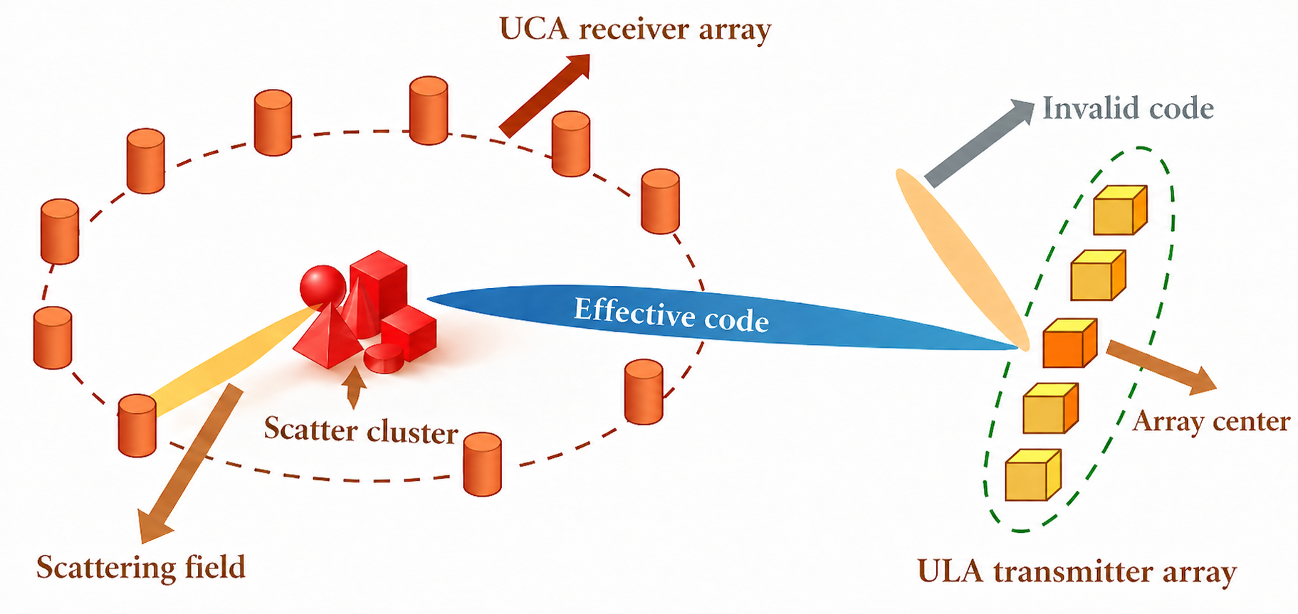
Let denote the geometric center of the transmit (TX) array, and let . The geometric departure angle associated with the -th cluster is then given by
| (64) |
where yields an angle of the complex number in .
Accordingly, the first step of the closed-loop beam-control pipeline returns a set of DT-inferred departure angles by selecting the most energetic clusters:
| (65) |
where returns the indices of the largest weights.
The DT-inferred departure-angle set provides a compact abstraction of the reconstructed propagation environment and serves as a natural interface between sensing and control, as shown in Fig. 2. Based on this propagation-aware representation, the closed-loop controller first performs a preprocessing step that uses to guide codebook-based beam preselection.
Consider a TX ULA with elements and half-wavelength spacing. The corresponding steering vector is defined as [34]
| (66) |
where is central wavelength, is the inter-element spacing, and denotes the centered element index given by
| (67) |
We define a predefined angular codebook consisting of uniformly spaced azimuth directions over as
| (68) |
where these angles represent geometric directions of departure, rather than the intrinsic steering angle domain of the array.
The TX BF codebook is then constructed as
| (69) |
For each codebook beam, we evaluate its matching score with the DT-inferred departure-angle set as
| (70) |
where denotes the -th codebook direction.
We then select beams with the largest scores, i.e.,
| (71) |
where denotes the index set of the selected beams.
This completes the first technical step of the proposed closed-loop beam-control framework, namely the identification of candidate beam directions for subsequent robust beam design.
IV-B Closed-Loop BF
The second technical step of the proposed closed-loop beam-control framework is to perform robust downlink BF based on the candidate beams identified in the preceding codebook-preselection step. The purpose of this step is not to introduce a new BF algorithm, but rather to provide a principled way of exploiting the DT-inferred cluster parameters to compute a TX beam under a limited on-air training budget.
With the dominant transmission directions explicitly characterized by the preceding codebook-preselection step, the BF design can be restricted to a low-dimensional subspace spanned by a subset of candidate beams. Specifically, let denote the index set of the shortlisted codewords, and collect the corresponding codewords into the matrix
| (72) |
The TX beamformer is then parameterized as a linear combination within this DT-informed subspace:
| (73) |
where is a low-dimensional coefficient vector.
Based on the reconstructed scattering clusters, we construct a frequency-dependent predicted MIMO channel as
| (74) |
where and denote the azimuth angle of arrival (AoA) and angle of departure (AoD) extracted from the reconstructed propagation geometry. Moreover, denotes the geometric delay of the -th cluster, where is the corresponding path length to the scattering center. The cluster-wise gain proxy is given by
| (75) |
where denotes the final contrast estimate.
For notational simplicity, the frequency argument is omitted below when no confusion arises.
The receive (RX) steering vector is computed in a coordinate-based manner from the calibrated RX array geometry returned by the -step.
Let denote the RX array center and be the calibrated coordinate of the -th element. Then,
| (76) | ||||
Assuming maximum-ratio combining (MRC) at the receiver, the predicted received signal-to-noise ratio (SNR) at frequency is
| (77) |
and the corresponding wideband SNR surrogate is
| (78) |
where denotes the set of considered frequency tones, and denotes the communication-noise power at the receiver.
Since is constructed from DT-estimated cluster parameters and calibrated geometry, inherits DT mismatch. We therefore adopt an outage-aware design [35]:
| (79) |
where denotes the target SNR threshold and is the allowable outage probability. Using a standard conservative sufficient condition based on one-sided concentration bounds, we obtain
| (80) |
where and are taken with respect to the DT-induced uncertainty. Equivalently, we maximize the risk-sensitive utility
| (81) |
Substituting yields a low-dimensional problem over the DT-informed subspace. Since is not necessarily column-orthonormal, we approximate the mean and variance terms by quadratic forms of while retaining a closed-form generalized eigen-solution. Define
| (82) | ||||
where captures the DT-induced uncertainty in the Gram domain. Importantly, the proposed GaBP-based DT construction primarily provides posterior mean estimates of the cluster parameters appearing in (74). Let collect the DT-estimated parameters of the dominant clusters, including the complex gain, delay, AoA, and AoD of each cluster. The covariance matrix quantifies the corresponding estimation uncertainty. We then obtain via first-order uncertainty propagation from . Specifically, define
| (83) |
Since , we partition row-wise according to the receive-antenna index as
| (84) |
where denotes the Jacobian block associated with the -th receive row of , and . Then, is approximated as
| (85) |
where and .
Under the subspace parameterization , both and admit quadratic approximations with respect to . Accordingly, the objective can be approximated as
| (86) |
with , where and denote the effective subspace matrices induced by and , respectively.
Consequently, the second step of the closed-loop beam-control design reduces to the following robust BF problem:
| (87) |
where
| (88) |
This yields the generalized eigenvalue problem whose solution is given by the dominant generalized eigenvector. Specifically,
| (89) |
From a control standpoint, the second step performs continuous beam refinement within the DT-informed subspace spanned by the shortlisted codewords obtained in the preceding preselection step. More broadly, the proposed closed-loop beam-control framework can be interpreted as a resource-reallocation mechanism: by leveraging DT priors to restrict the effective beam search space, the required pilot-signaling overhead is significantly reduced, while the complexity of DT reconstruction can be handled offline. In this sense, the framework trades offline computational resources for over-the-air training efficiency.
V Numerical Simulation Results
V-A Basic System Settings
This section evaluates DT construction under the GaBP framework, including scatterer reconstruction, array calibration, and DT-enabled closed-loop communication optimization.
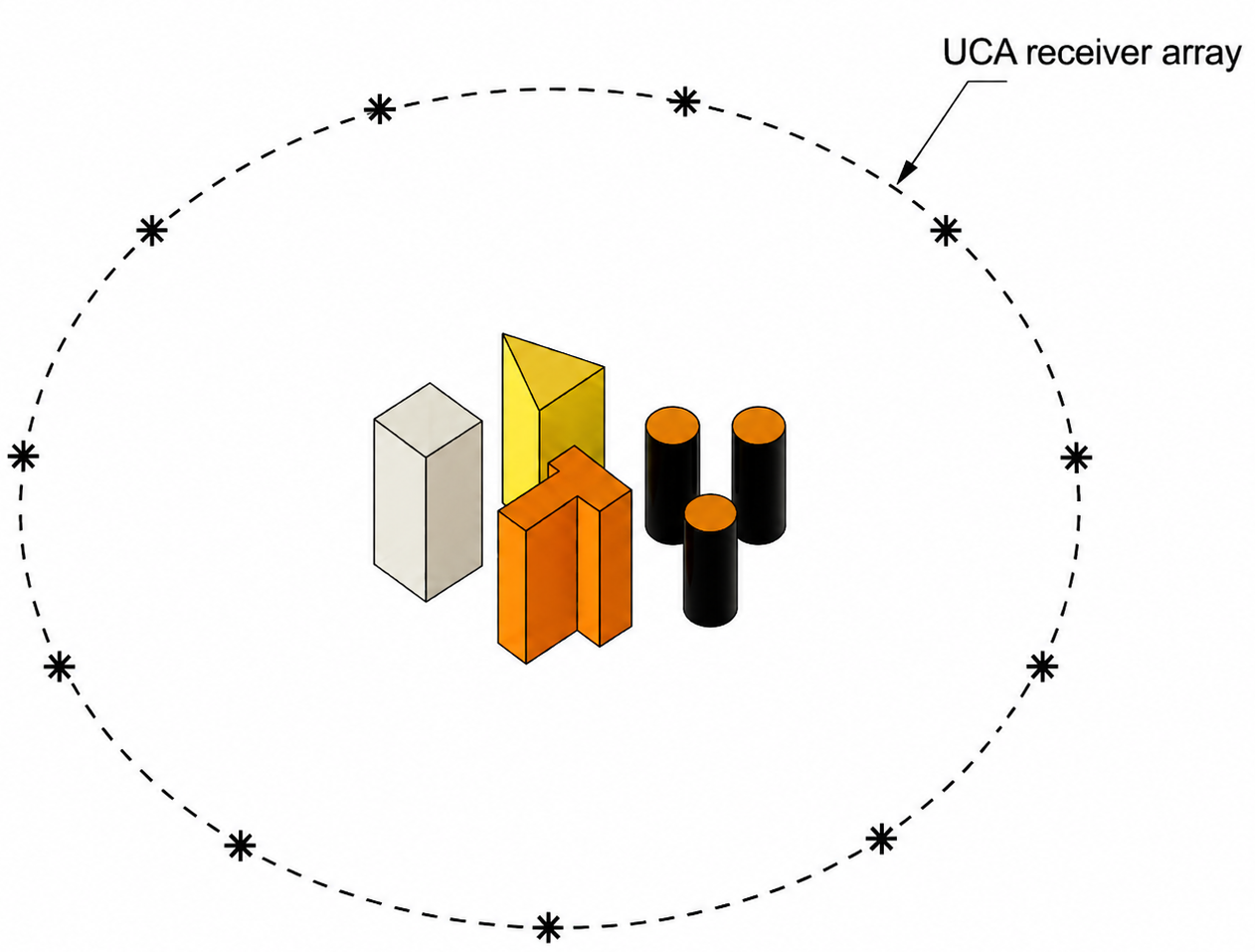
As shown in Fig. 2, the sensing region is and contains an equilateral triangle, a square, a T-shaped object, and a cluster of three small circular scatterers. Their characteristic dimensions are , , , and , respectively.
To evaluate the ability of GaBP to handle heterogeneous materials, three distinct material-parameter values are assigned to these scatterers. Each scatterer is assumed spatially homogeneous. Under the simplified TMz setting, all objects are uniform along the -direction with height .
The true antenna positions are generated by perturbing a nominal array geometry. The nominal RX array, also used as the inversion prior, is a UCA with elements on a circle of radius . The TX array is a ULA with elements and half-wavelength spacing at , located on the line and centered at .
To emulate array-position errors, independent truncated Gaussian perturbations in polar coordinates are applied to each element in both radius and angle, with standard deviations set to of the nominal radius and , respectively.
All electromagnetic field computations in the simulations are performed using the finite-difference time-domain (FDTD) method. Specifically, the sensing region is discretized into a grid. The OFDM carrier center frequency is set to , with subcarriers and subcarrier spacing .
V-B Scatterer Material Reconstruction


We evaluate material reconstruction under two sensing noise levels, and , which characterize the noise intensity in the electromagnetic sensing process and are distinct from the communication-link SNR defined later.
Fig. 4(a) shows the ground-truth 2-D material map: the triangle and square have , while the T-shape and the three-disk cluster have real-valued contrasts of and , respectively. Figs. 4(b) and (c) show the reconstructed maps obtained by the proposed GaBP with array calibration at sensing noise levels of and , respectively.
Under both weak-noise () and strong-noise () conditions, the proposed method accurately recovers the scatterer geometries while maintaining relatively small errors in the reconstructed material parameters. Note that antenna array calibration and material reconstruction are performed jointly in an alternating manner within the proposed GaBP framework, and the results shown here correspond to the converged material estimates after the joint calibration–reconstruction process.
In contrast, as shown in Fig. 4(d) and (e), an unresolved antenna array mismatch causes the -step in the GaBP algorithm to fail completely. In this case, the algorithm cannot recover the geometry or contrast distribution of any individual scatterer or scatterer cluster, and only spurious artifacts appear near the approximate scatterer locations. This behavior is caused by the use of an erroneous Green’s function, which significantly worsens the ill-conditioning of the overall forward operator and makes the solution of the associated linear system highly unstable. As a result, material reconstruction becomes infeasible under both weak- and strong-noise conditions.
Finally, Fig. 4(f) shows the NMSE performance of the -step in the GaBP algorithm as a function of the sensing noise level for cases with and without antenna array calibration. The NMSE of the reconstructed is defined as
| (90) |
When antenna array calibration is incorporated, the -step of the GaBP algorithm consistently achieves a low reconstruction error across different sensing noise levels, with the NMSE remaining around . As the sensing noise increases, the NMSE degrades by less than , indicating strong noise robustness of the calibrated -step.
In contrast, in the presence of an unresolved antenna array mismatch, material reconstruction becomes ineffective because of the severe mismatch in the forward operator. Consequently, the NMSE remains nearly constant across different noise levels, further highlighting the necessity of antenna array calibration in the proposed GaBP framework.

V-C Array Calibration
Following the material reconstruction results obtained in the -step, we next examine the performance of the proposed -step, which focuses on array calibration. In this and the subsequent subsection, all channel parameters are generated using the commercial ray-tracing simulator Wireless InSite, ensuring physically consistent propagation characteristics.
Fig. 5 shows the antenna array calibration results obtained in the -step under a sensing noise level of . The true antenna element positions are marked by blue crosses, the calibrated positions by red circles, and the prior (nominal) positions by orange circles. The estimated element locations closely match the true array geometry. After calibration, the NMSE of the antenna element positions relative to the true array geometry is reduced by in the radial domain and by in the angular domain, compared with the initial configuration.
The NMSE of the antenna array geometry is computed from the element-wise geometric deviations from the true array. Specifically, the NMSE in the radial and angular domains is defined as and , where and denote the true radial distance and angular position of the -th antenna element, respectively, while and are the corresponding calibrated estimates.
To further assess the accuracy of the calibrated antenna array at the channel level, the AoA and the power delay profile (PDP) are adopted as performance metrics.
As shown in Fig. 6(a), the AoA spectrum after calibration agrees much better with the reference distribution. Near the dominant component around , the calibrated spectrum matches both the reference peak location and its local shape, indicating accurate recovery of the main arriving direction. By contrast, the uncalibrated result in Fig. 6(b) is clearly distorted, with inconsistent peak prominence and spurious nearby components caused by array mismatch. In the – sector, where several strong components cluster and the spectrum becomes more structured, the calibrated curve preserves the reference envelope and peak concentration pattern, whereas the uncalibrated spectrum exhibits a clear shape mismatch, including exaggerated peaks and peak spreading. Overall, calibration substantially improves channel-level AoA fidelity, especially near and over –.
These gains are further supported by the AoA error cumulative distribution functions (CDFs) in Fig. 6(c) and Fig. 6(d). With calibration, the CDF nearly overlaps with the reference over the full range, particularly in the low-to-mid error region (roughly below ), indicating that most estimates have small angular deviations. Without calibration, the CDF shifts toward larger errors, with a clear gap in the mid-quantiles (about –) and a heavier tail, indicating more frequent large-angle outliers. Overall, array calibration suppresses large-error events and significantly improves AoA reliability.


As shown in Fig. 7(a), the calibrated PDP closely matches the ground-truth curve over most delay intervals. In the main multipath region (–), the two trajectories largely overlap, with typical deviations of about – across most delay bins. At larger delays (around –), discrepancies remain but are generally limited to about , with the largest local deviations reaching roughly –.
Without array calibration, as shown in Fig. 7(b), the PDP becomes strongly distorted in the delay tail. Around –, the uncalibrated PDP exhibits an artificial deep fade, dropping to about while the ground truth stays near to , i.e., a local error of roughly –. This suggests that array mismatch can severely corrupt multipath-energy estimation, especially at large delays.
The error CDFs in Fig. 7(c) and Fig. 7(d) further corroborate this trend. With calibration, the CDFs nearly coincide, and the horizontal gaps at the and quantiles are typically within –. Without calibration, the CDF shifts toward larger errors; for instance, near the quantile the gap increases to about –, indicating a heavier error tail in the uncalibrated case.
V-D DT-Guided Codebook Preselection

After the joint iterations of the -step and the -step have converged and reliable environment and array estimates are obtained, the system proceeds to the DT-guided codebook preselection stage. This subsection evaluates the effectiveness of the proposed DT-assisted codebook preselection strategy and compares it with the conventional exhaustive-search approach.
In the simulations, a uniform angular-domain codebook is adopted, where the beam directions are uniformly sampled from with a step size of , resulting in a total of codewords. For the exhaustive-search method, pilot signals are sequentially transmitted along all codeword directions in the codebook, and the codeword corresponding to the maximum received power is selected. In contrast, the DT-based method avoids full angular scanning by exploiting the prior geometric and environmental information provided by the constructed DT. Specifically, according to (71), a subset of the most relevant codewords is directly selected from the codebook. In the following experiments, the number of selected candidate codewords is set to .
Fig. 8 compares the codeword selection outcomes of the DT-assisted strategy and the conventional exhaustive-search benchmark. For the DT-based method, (71) yields a candidate set with codewords that captures the angular support inferred from the constructed DT. In the considered scenario, where the scattering energy is highly concentrated in angle, only the codeword pointing at within the candidate set corresponds to the dominant propagation direction, while the remaining candidates mainly serve to provide robustness against angular quantization and modeling uncertainties. By contrast, under the same air-interface budget, a No-DT baseline follows a fixed probing rule (three uniformly spaced beams and two midpoint refinements based on the summed feedback energy), which relies on coarse statistical priors and thus may miss the dominant direction. The exhaustive-search benchmark selects a codeword pointing at . Notably, the two selected directions differ by only one codeword step under the adopted angular resolution and therefore correspond to very similar beam directions with comparable link-level performance. Moreover, the geometric angle of the scatterer-region centroid relative to the TX array center is approximately , indicating that the codeword selected by the DT-based method is more consistent with the underlying scattering geometry. Overall, this result demonstrates that reliable codebook preselection can be achieved by exploiting DT-derived priors while operating on a significantly reduced candidate set.
V-E Closed-Loop Beam Management


After obtaining the DT-guided shortlisted codewords in the preceding subsection, we perform transmit beam optimization within this reduced candidate set, thereby completing the subsequent closed-loop beam-control procedure.
The gain of the proposed DT-guided strategy lies in an explicit resource tradeoff: offline computation for DT construction is used to reduce the over-the-air beam-sweeping burden. Under our experimental setting, DT construction takes approximately min, and the corresponding air-interface overhead reduction is depicted in Fig. 9.
We quantify the beam-training cost by the number of swept beams per beam-management cycle, i.e., the number of codewords that must be probed on the air interface to identify a suitable transmit beam. As shown in Fig. 9, decreasing the shortlist size leads to larger savings: the sweeping overhead scales with , whereas the reduction factor follows , where is the codebook size. In our implementation, the baseline probes all codewords, while the DT-guided scheme probes only shortlisted codewords for on-air confirmation, yielding a times reduction factor and an overhead saving. These results indicate that DT-guided inference can markedly reduce over-the-air sweeping while maintaining near-oracle BF performance.
Furthermore, to demonstrate the gain of DT-guided BF, we evaluate the received SNR and outage probability. Fig. 10 shows the per-antenna received SNR at the RX array for the calibrated and true arrays, with and without BF. Except for RX antenna index , BF improves the SNR by about – across most antennas. The SNR curves of the calibrated array closely match those of the true array, consistent with the high calibration accuracy reported earlier. For comparison, the green curve represents BF based on the original uncalibrated array geometry. Although it improves the SNR at some antennas, it also causes clear degradation at others. For example, at RX antenna index , the SNR decreases by compared with the no-BF case. This confirms the importance of accurate array geometry for spatially consistent BF performance.
Fig. 11 reports the outage probability as a function of the SNR threshold , where the dashed line highlights . It can be observed that the outage probability at is essentially zero for all configurations, indicating that the link reliably exceeds this threshold in the considered setup. As increases into the transition region (roughly –), applying BF consistently shifts the outage curves to the right, i.e., a lower outage is achieved at the same threshold. For example, around , BF reduces the outage probability by roughly – compared with the corresponding no-BF cases for both the calibrated-array and true-array settings. Moreover, the outage curves of the calibrated-array cases closely track those of the true-array cases, again confirming that the calibrated array yields channel-level performance that is highly consistent with the true array geometry. By contrast, BF based on the uncalibrated array geometry exhibits less consistent outage behavior because the reduced SNR at certain antennas increases the probability of falling below higher SNR thresholds.
VI Conclusion
This paper proposed an electromagnetic ISAC-assisted digital twin framework for antenna array calibration and DT-guided BF. By reconstructing a physically consistent digital twin that captures both the propagation environment and array geometry, the proposed approach mitigates array-manifold mismatch and supports more reliable model-based BF. More importantly, the proposed closed-loop architecture provides a resource-reallocation mechanism: rather than relying mainly on exhaustive over-the-air training, it leverages offline electromagnetic reconstruction and digital-twin inference to narrow the beam-management space and support downstream communication optimization. In this sense, the method effectively trades offline computational resources for air-interface resources, reducing online training overhead while maintaining robust BF performance. Overall, the results highlight the value of accurate DT reconstruction as a bridge from electromagnetic sensing to actionable communication control, thereby establishing a closed-loop link among environment perception, digital twin construction, and wireless system optimization.
References
- [1] X. Lin et al., “6G digital twin networks: From theory to practice,” IEEE Commun. Mag., vol. 61, no. 11, pp. 72–78, 2023.
- [2] M. Polese et al., “Colosseum: The Open RAN digital twin,” IEEE Open J. Commun. Soc., vol. 5, pp. 5452–5466, 2024.
- [3] Z. Zhang et al., “Digital twin-assisted data-driven optimization for reliable edge caching in wireless networks,” IEEE J. Sel. Areas Commun., vol. 42, no. 11, pp. 3306–3320, 2024.
- [4] M. Fahim et al., “Machine learning-based digital twin for predictive modeling in wind turbines,” IEEE Access, vol. 10, pp. 14184–14194, 2022.
- [5] L. Yu et al., “ChannelGPT: A large model toward real-world channel foundation model for 6G environment intelligence communication,” IEEE Commun. Mag., vol. 63, no. 10, pp. 68–74, 2025.
- [6] L. Li et al., “Digital twins of electromagnetic propagation environments for live 5G networks—Part I: Channel acquisition, EM simulation, and verification,” IEEE Trans. Antennas Propag., vol. 73, no. 4, pp. 2053–2064, 2025.
- [7] Y. Jiang et al., “Electromagnetic property sensing: A new paradigm of integrated sensing and communication,” IEEE Trans. Wireless Commun., vol. 23, no. 10, pp. 13471–13483, Oct. 2024.
- [8] Y. Jiang et al., “Electromagnetic property sensing in ISAC with multiple base stations: Algorithm, pilot design, and performance analysis,” IEEE Trans. Wireless Commun., 2025.
- [9] Y. Jiang et al., “Electromagnetic property sensing and channel reconstruction based on diffusion Schrödinger bridge in ISAC,” IEEE Trans. Wireless Commun., vol. 24, no. 8, pp. 6737–6752, 2025.
- [10] Y. Luo et al., “Ill-posedness analysis of CSI-based electromagnetic inverse scattering for material reconstruction in ISAC systems,” arXiv preprint arXiv:2603.05918, 2026.
- [11] L. Wen et al., “Inverse scattering approach to integration of communication and sensing,” IEEE J. Sel. Top. Electromagn., Antennas Propag., vol. 1, no. 1, pp. 20–36, 2025.
- [12] W. Cai et al., “Beam prediction based on multi-modal joint environment sensing,” IEEE Wireless Commun. Lett., vol. 15, pp. 1722–1726, 2026.
- [13] H. Wang et al., “Digital twin channel for 6G: Concepts, architectures and potential applications,” IEEE Commun. Mag., vol. 63, no. 3, pp. 24–30, 2025.
- [14] J. Geiss et al., “The impact of antenna array calibration errors on MIMO and multi-channel synthetic aperture radar imaging,” IEEE J. Microw., vol. 3, no. 2, pp. 635–654, Apr. 2023.
- [15] H. Hoang et al., “Calibration to mitigate near-field antennas effects for a MIMO radar imaging system,” Sensors, vol. 21, no. 2, Art. no. 514, Jan. 2021.
- [16] Z. Zhu et al., “Coupled phase-shift STAR-RIS for secure MIMO communication: A DRL-based BF design,” IEEE Commun. Lett., vol. 28, no. 11, pp. 2488–2492, Nov. 2024.
- [17] Y. Kabashima, “A CDMA multiuser detection algorithm on the basis of belief propagation,” J. Phy. A: Math. and Gen., vol. 36, no. 43, pp. 11111–11121, Oct. 2003.
- [18] T. Takahashi et al., “Design of adaptively scaled belief in multi-dimensional signal detection for higher-order modulation,” IEEE Trans. Wireless Commun., vol. 67, no. 3, pp. 1986–2001, Mar. 2019.
- [19] D. Bickson et al., “Gaussian belief propagation: Theory and application,” IEEE Trans. Signal Process., vol. 59, no. 5, pp. 2163–2178, May 2011.
- [20] D. Ma et al., “Inverse scattering-enabled integration of sensing, identification, and backscatter communication for near-field driven 6G networks,” IEEE Netw., vol. 39, no. 6, pp. 21–29, Nov. 2025.
- [21] J. Zhu et al., “Electromagnetic information theory-based statistical channel model for improved channel estimation,” IEEE Trans. Inf. Theory, vol. 71, no. 3, pp. 1777–1793, 2025.
- [22] Y. Luo et al., “A robust CSI-based scatterer geometric reconstruction method for 6G ISAC system,” IEEE Wireless Commun. Lett., vol. 15, pp. 2129–2133, 2026.
- [23] K. Ito et al., “Bilinear Gaussian Belief Propagation for Massive MIMO Detection With Non-Orthogonal Pilots,” IEEE Trans. Commun., vol. 72, no. 2, pp. 1045–1061, Feb. 2024.
- [24] T. Takahashi et al., “Bayesian receiver design via bilinear inference for cell-free massive MIMO with low-resolution ADCs,” IEEE Trans. Wireless Commun., vol. 22, no. 7, pp. 4756–4772, Jul. 2023.
- [25] H. Iimori et al., “Grant-free access via bilinear inference for cell-free MIMO with low-coherence pilots,” IEEE Trans. Wireless Commun., vol. 20, no. 11, pp. 7694–7710, Nov. 2021.
- [26] T. Furudoi et al., “Discrete-valued signal estimation via low-complexity message passing algorithm for highly correlated measurements,” arXiv preprint arXiv:2411.07558, 2024.
- [27] D. Liu et al., “Multi-frequency neural Born iterative method for solving 2-D inverse scattering problems,” IEEE Trans. Comput. Imag., vol. 11, pp. 1243–1257, 2025.
- [28] A. Costa Batista et al., “A quadratic programming approach for microwave imaging,” IEEE Trans. Antennas Propag., vol. 69, no. 8, pp. 4923–4934, Aug. 2021.
- [29] D. Colton et al., Inverse Acoustic and Electromagnetic Scattering Theory, 3rd ed. New York, NY, USA: Springer, 1998.
- [30] X. Wang et al., “Beam management for millimeter-wave communications with integrated sensing and communication,” IEEE Trans. Wireless Commun., vol. 22, no. 2, pp. 1315–1329, Feb. 2023.
- [31] P. M. Meaney et al., “Microwave imaging for breast cancer detection,” IEEE Trans. Microw. Theory Techn., vol. 48, no. 11, pp. 1841–1853, Nov. 2000.
- [32] A. Alkhateeb et al., “Channel estimation and hybrid precoding for millimeter wave cellular systems,” IEEE J. Sel. Topics Signal Process., vol. 8, no. 5, pp. 831–846, Oct. 2014.
- [33] A. Weiss et al., “Array shape calibration using sources in unknown locations,” IEEE Trans. Signal Process., vol. 47, no. 5, pp. 1399–1412, May 1999.
- [34] T. S. Rappaport et al., “Millimeter wave wireless communications,” IEEE Commun. Mag., vol. 52, no. 9, pp. 40–48, Sep. 2014.
- [35] A. Gershman et al., “Convex optimization-based BF,” IEEE Signal Process. Mag., vol. 27, no. 3, pp. 62–75, May 2010.