Structure-Informed Bounds on the Kronecker Rank of Block-Structured Matrices

The Kronecker product of $\mathbf{C}\in\mathbb{R}^{\ell\times q}$ and $\mathbf{D}\in\mathbb{R}^{m\times n}$ is the $(\ell m)\times(qn)$ matrix

$$\mathbf{C}\otimes\mathbf{D}=\begin{bmatrix}c_{11}\mathbf{D}&\cdots&c_{1q}\mathbf{D}\\ \vdots&\ddots&\vdots\\ c_{\ell 1}\mathbf{D}&\cdots&c_{\ell q}\mathbf{D}\end{bmatrix}.$$

The following properties will be used throughout [Ballard_Kolda_2025, graham2018kronecker, vanloan2000ubiquitous, magnus1979commutation]:

1. 1.

   $(\mathbf{C}\otimes\mathbf{D})^{\top}=\mathbf{C}^{\top}\otimes\mathbf{D}^{\top}$.

2. 2.

   $\mathbf{C}\otimes(\mathbf{D}+\mathbf{E})=(\mathbf{C}\otimes\mathbf{D})+(\mathbf{C}\otimes\mathbf{E})$.

3. 3.

   $(\mathbf{C}\otimes\mathbf{D})\mathbf{x}=\mathrm{vec}(\mathbf{D}\mathbf{X}\mathbf{C}^{\top})$, where $\mathbf{x}=\mathrm{vec}(\mathbf{X})$ and $\mathrm{vec}(\cdot)$ stacks columns.

4. 4.

   There exist permutation matrices $\mathbf{P}$ and $\mathbf{Q}$ such that

   $$\mathbf{P}(\mathbf{C}\otimes\mathbf{D})\mathbf{Q}^{\top}=\mathbf{D}\otimes\mathbf{C},$$

   where $\mathbf{P}=\mathbf{S}_{\ell,m}$, $\mathbf{Q}=\mathbf{S}_{q,n}$, and

   (1)

   $$\mathbf{S}_{a,b}=\begin{bmatrix}[\mathbf{I}_{s}]_{1:b:s,:}\\ [\mathbf{I}_{s}]_{2:b:s,:}\\ \vdots\\ [\mathbf{I}_{s}]_{b:b:s,:}\end{bmatrix},\quad s=ab.$$

We use tensor to denote a multiway array; unless otherwise stated, all tensors are third-order. By fixing all but one index of $\mathbf{\mathcal{A}}$, we obtain fibers; by fixing all but two indices, we obtain two-dimensional slices [kolda2009tensor] (see Figure 1). We write $\mathbf{A}^{[k]}=\mathbf{\mathcal{A}}_{:,:,k}$ for the $k$th frontal slice and $\overrightarrow{\mathbf{\mathcal{A}}}_{j}=\mathbf{\mathcal{A}}_{:,j,:}$ for the $j$th lateral slice. The operators $\mathtt{twist}(\cdot)\colon\mathbb{R}^{m\times p\times 1}\to\mathbb{R}^{m\times 1\times p}$ and $\mathtt{squeeze}(\cdot)\colon\mathbb{R}^{m\times 1\times p}\to\mathbb{R}^{m\times p\times 1}$ reorient frontal slices as lateral slices and vice versa [kilmer2013TensorOperator]. See Figure 2 for a visualization of these operators.

The mode-$i$ unfolding $\mathbf{A}_{(i)}$ is formed by arranging mode-$i$ fibers as columns. For $\mathbf{\mathcal{A}}\in\mathbb{R}^{m\times p\times n}$:

	$\displaystyle\mathbf{A}_{(1)}$	$\displaystyle=\bigl[\mathbf{A}^{[1]},\,\mathbf{A}^{[2]},\,\dots,\,\mathbf{A}^{[n]}\bigr]\in\mathbb{R}^{m\times pn},$
	$\displaystyle\mathbf{A}_{(2)}$	$\displaystyle=\bigl[(\mathbf{A}^{[1]})^{\top},\,(\mathbf{A}^{[2]})^{\top},\,\dots,\,(\mathbf{A}^{[n]})^{\top}\bigr]\in\mathbb{R}^{p\times mn},$
	$\displaystyle\mathbf{A}_{(3)}$	$\displaystyle=\bigl[\mathtt{squeeze}(\overrightarrow{\mathbf{\mathcal{A}}}_{1}^{\top}),\,\dots,\,\mathtt{squeeze}(\overrightarrow{\mathbf{\mathcal{A}}}_{p}^{\top})\bigr]\in\mathbb{R}^{n\times mp}.$

The multirank of $\mathbf{\mathcal{A}}$ is $(r_{1},r_{2},r_{3})$ with $r_{i}=\mathrm{rank}(\mathbf{A}_{(i)})$. Mode-$i$ multiplication is defined by $\mathbf{\mathcal{C}}=\mathbf{\mathcal{A}}\times_{i}\mathbf{B}\Leftrightarrow\mathbf{C}_{(i)}=\mathbf{B}\mathbf{A}_{(i)}$.

The Tucker decomposition of $\mathbf{\mathcal{A}}\in\mathbb{R}^{m\times p\times n}$ is defined by

$$\mathbf{\mathcal{A}}=\mathbf{\mathcal{G}}\times_{1}\mathbf{U}\times_{2}\mathbf{V}\times_{3}\mathbf{W},$$

where $\mathbf{U}\in\mathbb{R}^{m\times r_{1}}$, $\mathbf{V}\in\mathbb{R}^{p\times r_{2}}$, $\mathbf{W}\in\mathbb{R}^{n\times r_{3}}$, and the core tensor $\mathbf{\mathcal{G}}\in\mathbb{R}^{r_{1}\times r_{2}\times r_{3}}$ [kolda2009tensor]. One method for computing this decomposition is the higher-order SVD (HOSVD) [delathauwer2000hosvd], outlined in Algorithm 1.

When the multirank is much smaller than the tensor dimensions, the HOSVD provides an implicitly compressed representation. In this work, we focus on the exact HOSVD and, in particular, on bounds for $r_{2}$, which will be shown to equal the Kronecker rank.

We now review the construction of Kilmer and Saibaba [kilmer2022matrixtensordecomp]. Let $\mathbf{A}\in\mathbb{R}^{(\ell m)\times(qn)}$ be a block-structured matrix with $p$ distinct blocks $\mathbf{A}_{k}\in\mathbb{R}^{m\times n}$, $k=1,\dots,p$. Define the location-tally matrices $\mathbf{E}_{k}\in\mathbb{R}^{\ell\times q}$ by

(2)

$$[\mathbf{E}_{k}]_{ij}=\begin{cases}1/\sqrt{\eta_{k}}&\text{if block }\mathbf{A}_{k}\text{ occurs at block position }(i,j),\\ 0&\text{otherwise,}\end{cases}$$

where $\eta_{k}$ is the number of occurrences of $\mathbf{A}_{k}$. Then,

(3)

$$\mathbf{A}=\sum_{k=1}^{p}\mathbf{E}_{k}\otimes\sqrt{\eta_{k}}\mathbf{A}_{k}.$$

A visual representation of Equation (3) is given in Figure 3 for a block-symmetric block-Toeplitz matrix $\mathbf{A}$ with three distinct blocks.

The matrix-to-tensor map $\mathcal{T}\colon\mathbb{R}^{(\ell m)\times(qn)}\to\mathbb{R}^{m\times p\times n}$ is defined by setting the $k$th lateral slice of $\mathbf{\mathcal{A}}:=\mathcal{T}[\mathbf{A}]$ to

(4)

$$\overrightarrow{\mathbf{\mathcal{A}}}_{k}=\mathtt{twist}(\sqrt{\eta_{k}}\mathbf{A}_{k}),\quad k=1,\dots,p.$$

The inverse tensor-to-matrix map $\mathcal{M}\colon\mathbb{R}^{m\times p\times n}\to\mathbb{R}^{(\ell m)\times(qn)}$ is

$$\mathcal{M}[\mathbf{\mathcal{A}}]=\sum_{k=1}^{p}\mathbf{E}_{k}\otimes\mathtt{squeeze}(\overrightarrow{\mathbf{\mathcal{A}}}_{k}).$$

If $\mathbf{\mathcal{A}}$ admits the Tucker decomposition $\mathbf{\mathcal{A}}=\mathbf{\mathcal{G}}\times_{1}\mathbf{U}\times_{2}\mathbf{V}\times_{3}\mathbf{W}$ with $\mathbf{\mathcal{G}}\in\mathbb{R}^{r_{1}\times r_{2}\times r_{3}}$, then

(5)

$$\mathbf{A}=\mathcal{M}[\mathbf{\mathcal{A}}]=\sum_{j=1}^{r_{2}}\mathbf{C}_{j}\otimes\mathbf{D}_{j},$$

where $\mathbf{C}_{j}=\sum_{k=1}^{p}v_{kj}\mathbf{E}_{k}$, $\mathbf{D}_{j}=\mathbf{U}\mathbf{G}_{j}\mathbf{W}^{\top}$, $v_{kj}=[\mathbf{V}]_{kj}$, and $\mathbf{G}_{j}=\mathtt{squeeze}(\overrightarrow{\mathbf{\mathcal{G}}}_{j})$. The integer $r_{2}$ is thus the number of terms in the Kronecker sum produced by this framework. Figure 4 illustrates the full pipeline.

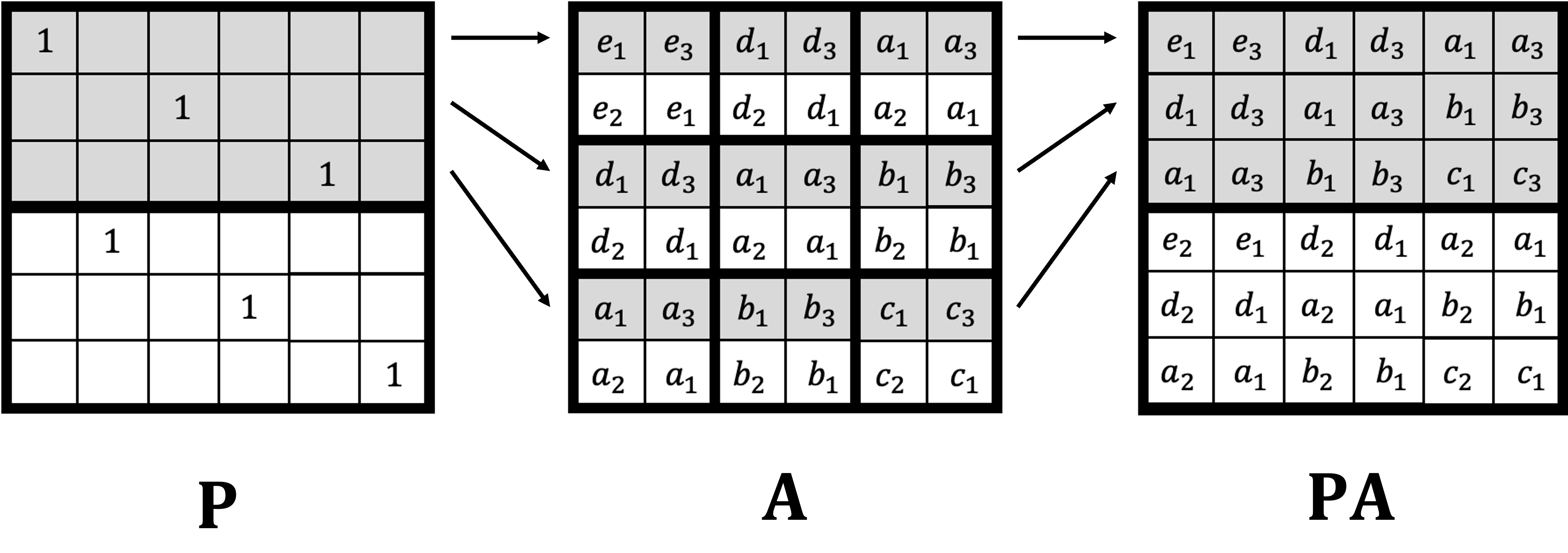
By property 4 of the Kronecker product, there exist permutation matrices $\mathbf{P}\in\mathbb{R}^{(\ell m)\times(\ell m)}$ and $\mathbf{Q}\in\mathbb{R}^{(qn)\times(qn)}$ with $\mathbf{P}=\mathbf{S}_{\ell,m}$ and $\mathbf{Q}=\mathbf{S}_{q,n}$ such that

$$\mathbf{P}(\mathbf{E}_{k}\otimes\sqrt{\eta_{k}}\mathbf{A}_{k})\mathbf{Q}^{\top}=\sqrt{\eta_{k}}\mathbf{A}_{k}\otimes\mathbf{E}_{k}.$$

Define $\mathbf{B}=\mathbf{P}\mathbf{A}\mathbf{Q}^{\top}\in\mathbb{R}^{(m\ell)\times(nq)}$. This matrix is block-structured with an $m\times n$ grid of blocks each of size $\ell\times q$, and satisfies

(6)

$$\mathbf{A}=\mathbf{P}^{\top}\mathbf{B}\mathbf{Q}=\sum_{\kappa=1}^{\rho}\sqrt{\xi_{\kappa}}\mathbf{B}_{\kappa}\otimes\mathbf{F}_{\kappa},$$

where $\mathbf{B}_{\kappa}\in\mathbb{R}^{\ell\times q}$ are the $\rho$ distinct blocks of $\mathbf{B}$, $\xi_{\kappa}$ is the multiplicity of $\mathbf{B}_{\kappa}$, and $\mathbf{F}_{\kappa}\in\mathbb{R}^{m\times n}$ is the corresponding location-tally matrix. We use $k,p$ for counts associated with $\mathbf{A}$ and $\kappa,\rho$ for those associated with $\mathbf{B}$.

Let $(\alpha,\beta)\in[m]\times[n]$ and $(\gamma,\delta)\in[\ell]\times[q]$. Let $\mathbf{A}^{(\gamma,\delta)}$ denote the block of $\mathbf{A}$ in block-location $(\gamma,\delta)$, and $\mathbf{B}^{(\alpha,\beta)}$ the block of $\mathbf{B}$ in block-location $(\alpha,\beta)$. The following lemma makes the element-wise relationship between $\mathbf{A}$ and $\mathbf{B}$ precise.

In the example of Figure 5, one may verify directly that $\mathbf{A}^{(2,1)}_{2,2}=\mathbf{B}^{(2,2)}_{2,1}=d_{1}$, consistent with (7).

Let $A=\{\mathbf{A}_{k}\}_{k=1}^{p}$ be the set of distinct blocks of $\mathbf{A}$, let $E=\{\mathbf{E}_{k}\}_{k=1}^{p}$ be the associated location-tally matrices, let $B=\{\mathbf{B}_{\kappa}\}_{\kappa=1}^{\rho}$ be the distinct blocks of $\mathbf{B}$, and let $F=\{\mathbf{F}_{\kappa}\}_{\kappa=1}^{\rho}$ be the corresponding tally matrices.

Because $\mathbf{A}=\mathbf{P}^{\top}\mathbf{B}\mathbf{Q}$, we can write $\mathbf{A}$ as a sum of $r_{2}$ or $\bar{r}_{2}:=\dim(\mathscr{B})$ Kronecker products. The following theorem shows that these two quantities coincide.

The first proof establishes the equality by a dimension argument. Here we give a second proof by showing that the outer blockspan $\mathscr{B}$ is isomorphic to the column space of $\mathbf{A}_{(2)}$, whose dimension is $r_{2}=\dim(\mathscr{A})$ by Theorem 4.1.

Recall from the proof of Proposition 3.5 that each $\mathbf{B}_{\kappa}\in B$ satisfies $\mathbf{B}_{\kappa}=\sum_{k=1}^{p}b_{\kappa}^{k}(\sqrt{\eta_{k}}\mathbf{E}_{k})$. Define two linear maps:

(13)

$$\mathtt{vec}_{\mathscr{E}}(\mathbf{B}_{\kappa})=\begin{bmatrix}\sqrt{\eta_{1}}b_{\kappa}^{1}\\ \vdots\\ \sqrt{\eta_{p}}b_{\kappa}^{p}\end{bmatrix}\in\mathbb{R}^{p}\quad\mbox{ and }\quad\mathtt{mat}_{\mathscr{E}}(\mathbf{v})=\sum_{k=1}^{p}v_{k}\mathbf{E}_{k},\quad\mathbf{v}\in\mathbb{R}^{p}.$$

Both maps extend linearly to their respective domains.

Theorem 4.4 follows immediately: $\dim(\mathscr{B})=\dim(\mathrm{colspace}(\mathbf{A}_{(2)}))=r_{2}=\dim(\mathscr{A})$.

From Theorem 4.1, the Kronecker rank $r_{2}=\dim(\mathscr{A})$. When the blocks of $\mathbf{A}$ are not known explicitly, one can bound $\dim(\mathscr{A})$ by working with larger spaces defined by the structural type of the blocks.

Let $\mathscr{S}$ denote the subspace of matrices whose form is determined by the structural type of the blocks of $\mathbf{A}$ (e.g., the space of $m\times n$ Toeplitz matrices if each block is Toeplitz), and let $\mathscr{T}$ denote the analogous space for the outer block structure (i.e., the structural type of the blocks of $\mathbf{B}$). By construction, $\mathscr{A}\subseteq\mathscr{S}\subseteq\mathscr{F}$ and $\mathscr{B}\subseteq\mathscr{T}\subseteq\mathscr{E}$.

Figure 8 illustrates these containments.

When the blocks of $\mathbf{A}$ are sparse, the rank of $\mathbf{A}_{(2)}$ is bounded by the number of positions that are nonzero in at least one block. This is formalized in the following theorem.

When all blocks share the same sparsity pattern, $\bigcup_{k}C_{k}=C_{k}$ for any $k$, so $r_{2}\leq\mathtt{nnz}(\mathbf{A}_{k})$. For banded blocks, the following corollary applies immediately.

We can also establish a relationship between the sparsity within the blocks of $\mathbf{A}$ and the block-sparsity of the permuted matrix $\mathbf{B}$. Here, block-sparsity refers to the ratio of nonzero blocks to the total number of blocks. To do so, we present the following theorem.

Matrices with Block-Toeplitz-plus-Hankel structure with Toeplitz-plus-Hankel blocks (BTHTHB) arise in image deblurring [hansen2006deblur, kilmer2007tplush, nagy2004reflexivekron]. We verify Corollary 5.1 by comparing the theoretical bound $r_{th}$ (derived from structure) with the numerically computed rank $r_{calc}=\mathrm{rank}(\mathbf{A}_{(2)})$ for four BTHTHB structures.

Let $\mathbf{A}\in\mathbb{R}^{n^{2}\times n^{2}}$ be BTHTHB with $n\times n$ blocks and random entries, so that any dependence among the blocks of $\mathbf{A}$ is attributable to structure alone. Write $\mathbf{A}=\mathbf{A}_{T}+\mathbf{A}_{H}$ where $\mathbf{A}_{T}$ is block-Toeplitz and $\mathbf{A}_{H}$ is block-Hankel. Letting $\nu\sim\mathcal{N}(0,1)$ independently, we construct

$$\mathbf{A}=\Bigl(\sum_{i}\tilde{\mathbf{E}}_{T_{i}}\otimes\sum_{j}\nu_{j}\tilde{\mathbf{E}}_{T_{j}}\Bigr)+\Bigl(\sum_{k}\tilde{\mathbf{E}}_{H_{k}}\otimes\sum_{\ell}\nu_{\ell}\tilde{\mathbf{E}}_{H_{\ell}}\Bigr),$$

where $\tilde{\mathbf{E}}_{(\cdot)}$ are the unscaled location-tally matrices. The four structures tested (illustrated in Figure 9) are:

• •

  Symmetric Full: $\mathbf{A}_{T}$ full and block-symmetric and $\mathbf{A}_{H}$ full and block-persymmetric.

• •

  Nonsymmetric Full: same, without symmetry or persymmetry.

• •

  Symmetric Banded: $\mathbf{A}_{T}$ block-banded with upper bandwidth $n/2-1$, lower bandwidth $n/2$ (nearly symmetric); $\mathbf{A}_{H}$ analogously banded (nearly persymmetric).

• •

  Nonsymmetric Banded: as above, without the symmetry conditions.

The results are shown in Table 2. In the center columns, we compare $r_{th}$ to $p$ and $r_{calc}$, the rank of $\mathbf{A}_{(2)}$ as calculated by the MATLAB $\mathtt{rank}$ command. Agreement $r_{th}=r_{calc}$ holds in all cases, confirming that our structural bounds are exact. The relative error between $\mathbf{A}$ and the reconstruction $\tilde{\mathbf{A}}$ using only $r_{th}$ Kronecker terms was on the order of $10^{-15}$ in all cases.