跳到论文正文
W Papers独立论文阅读器 arXiv:2605.29669 论文正文 计算阅读时间 · 0%
引用这篇论文根据当前论文元数据生成,正式投稿前建议核对。


License: CC BY 4.0
arXiv:2605.29669v2 [stat.ML] 16 Jun 2026

Eigen-Spike Emergence and Quadratic Equivalents for Conjugate Kernels on Nonlinearly Separable Data

Collin Cranston∗ Department of Mathematics University of California San Diego USA
ccransto@ucsd.edu Zhichao Wang∗ ICSI and Department of Statistics University of California
Berkeley USA
zhichao.wang@berkeley.edu Todd Kemp Department of Mathematics University of California
San Diego USA
tkemp@ucsd.edu Michael W. Mahoney ICSI
LBNL and Department of Statistics
University of California
Berkeley USA
mmahoney@stat.berkeley.edu
Abstract

Recent work in random matrix theory (RMT) has developed the notion of deterministic equivalents: typically linear surrogate models that approximate the spectral behavior of large nonlinear random matrices, such as nonlinear feature maps in neural networks (NNs). Such equivalents make theoretical predictions tractable by reducing a complex model to a simpler one with properties that fall under the umbrella of classical RMT tools. However, this leaves open the question of whether this idealized linear equivalence remains meaningful for classification of high-dimensional nonlinearly separable data. Motivated by this, we consider the conjugate kernel (CK), which is the nonlinear feature map of a one-layer feedforward NN, under a canonical nonlinearly separable dataset for the XOR problem; and we use the study of informative outlier eigenvalues in the CK and whether their corresponding eigenvectors asymptotically align with XOR labels as a proxy for nonlinear learnability. We develop a robust quadratic equivalent of the CK matrix that enables a precise analysis of emergent informative spikes, as one modifies various knobs common in ML practice: sample complexity, signal-to-noise ratio (SNR), nonlinear activation choice, and pretrained features. We identify regimes in which these knobs move the CK beyond the linear equivalent and produce BBP-type transitions to label-aligned outlier eigenspaces. Our analysis helps bring deterministic-equivalence tools from RMT to bear on problems of practical relevance in ML.

††footnotetext: ∗Equal contribution.

1 Introduction

Spectral information from weight matrices, kernel matrices, and Hessians provides a quantitative window into representation learning and efficient optimization in neural networks (NNs) [MM21, MM19, MM20, MPM21, YTH+22, WES+23, JGH18, PW17, AP20, LM21, SBL16, GKX19a]. For example, eigenvalues of NN weight matrices can capture the strength of learned directions, while the corresponding eigenvectors indicate which data features are amplified or extracted during training [BES+22, DLS22, MLH+23, DPC+24]. A major direction in deep learning theory is to use spectral tools to understand when NNs can propagate, preserve, transform, or amplify task-relevant structure that may be hidden in high-dimensional datasets.

A concrete and widely used spectral mechanism is the emergence of spikes (outlier eigen/singular values) and the alignment of their eigen/singular vectors with signals in the dataset. Random matrix theory (RMT) provides a powerful tool to analyze such eigen-spike emergence. In high-dimensional spiked models where a low-rank signal is embedded in Gaussian noise, BBP (Baik–Ben Arous–Péché) phase transitions characterize when an informative outlier separates from the bulk spectrum and when its associated eigenvector becomes correlated with the underlying signal [BAP05, NAD08]. Recent work has developed nonlinear counterparts for random-feature and kernel-type matrices, providing sharp predictions for outlier locations and eigenvector alignment [FEL23, BES+22, BES+23, WWF24]. Such nonlinear RMT can be applied to study deep learning theory, e.g., the infinite-width Neural Tangent Kernel (NTK) and the Conjugate Kernel (CK) [JGH18, PW17, AP20] for multi-layer NNs. Their high-dimensional spectra have been studied extensively [LM25, WZ24, LCM20]. In this work, we focus on the CK, and we study emergent spikes induced by nonlinear structure in the data. Concretely, we consider the following spectral question for CK:

When can NNs transfer a nonlinear pattern in the data into a linearly accessible direction (an aligned eigen-spike) that enables linear classification?

In this paper, the CK is defined by a one-hidden-layer random NN: 𝒀=1N​σ​(𝑾​𝑿)∈ℝN×n,\bm{Y}=\frac{1}{\sqrt{N}}\,\sigma(\bm{W}\bm{X})\in\mathbb{R}^{N\times n}, with nonlinear activation σ\sigma, random weights 𝑾∈ℝN×d\bm{W}\in\mathbb{R}^{N\times d}, and data 𝑿∈ℝd×n\bm{X}\in\mathbb{R}^{d\times n}. The CK matrix is the Gram matrix of hidden activations, 𝑲=𝒀⊤​𝒀∈ℝn×n\bm{K}=\bm{Y}^{\top}\bm{Y}\in\mathbb{R}^{n\times n} for nn data points. The spectral distribution of 𝑲\bm{K} is particularly useful for generalization error of random feature regression, as demonstrated in [MM22, HL22] for isotropic Gaussian data 𝑿\bm{X}. However, real datasets often contain low-rank or nonlinear structure that may be hard to analyze using PCA [JOL02, SSM98, TdL00, RS00, BN03, CL06, JL09]. To highlight genuinely nonlinear structure, we instead take 𝑿\bm{X} to be the high-dimensional XOR Gaussian mixture dataset (Section 3). This dataset is a balanced four-component Gaussian mixture whose two classes are unions of opposite components [RGK+21]. The key property is that XOR is not linearly separable in first-order statistics: the class means vanish, and any method that only “sees” linear correlations cannot recover labels. However, XOR is quadratically separable, so a second-order feature can potentially make the task linearly solvable. Heuristically, the eigenvalues of 𝑲\bm{K} describe the spectrum of learned similarities, while the alignment of leading eigenvectors with task structure (e.g., labels or cluster indicators) may lead to spectral methods solving the task. Therefore, this paper aims to answer the following spectral question for 𝑲\bm{K}:

When do outlier eigenvalues emerge in the CK spectrum, and when do their spiked eigenvectors align with the XOR labels and enable linear classification?

In practice, NN performance is affected by hyperparameters, dataset structure, and architecture; and, as a practical matter, machine learning (ML) practitioners typically fiddle (quite aggressively) with various “knobs” of the ML training process in order to improve model performance. Motivated by this, we consider properties of the CK matrix for the XOR problem, as various “knobs” for 𝑲\bm{K} are varied; and, depending on their values, we observe very different spectral behavior. Concretely, we vary the following knobs (which are among the standard parameters that are tuned in ML practice): sampling size scaling nn with input features dd and NN width NN; signal-to-noise ratio (SNR) in the data 𝑿\bm{X}; the pretrained weight matrix 𝑾\bm{W}; and the choice of nonlinear activation σ\sigma. We show that, depending on the values of these “knobs,” one can obtain qualitatively different spectral properties, various phase transitions, and the emergence of quadratic informative spikes in the CK matrix. Importantly, the emergence of these quadratically informative spikes makes the nonlinear XOR linearly classifiable.

Refer to caption
Refer to caption
Figure 1: Finite-SNR proportional regime: linear classification of XOR fails. Spectrum of the random CK matrix 𝑲\bm{K} built from XOR data with n=5000n=5000, N=d=15000N=d=15000, SNR r2=36r^{2}=36, and σ∝ReLU\sigma\propto\mathrm{ReLU}. Left: empirical eigenvalue histogram of 𝑲\bm{K} (blue) against the deformed MP law predicted by Theorem 3 (red curve); the red ×\color[rgb]{1,0,0}{\times} marks the predicted location of the two (coincident) outlier eigenvalues and the dashed lines mark the empirical values. The subfigure plots the two outlier eigenvectors against sample index, showing four-block pattern of the Gaussian-mixture components but not the binary labels. Right: kernel-PCA embedding using the top two principal components (PCs) of 𝑲\bm{K} (one point per sample, colored by its true label); the four clouds form the canonical XOR geometry and are not linearly separable. The outlier eigenspace is asymptotically orthogonal to XOR label vector 𝒚{\bm{y}} in this baseline case.

1.1 Our Approach

Much of the existing RMT literature on the CK matrix analysis lies in a proportional regime (n≍d≍Nn\asymp d\asymp N), and it often involves the assumption of isotropic Gaussian data 𝒁∈ℝd×n\bm{Z}\in\mathbb{R}^{d\times n}. In this setting, a standard tool is a linear equivalent (LE) for the nonlinear feature matrix σ​(𝑾​𝒁)\sigma(\bm{W}\bm{Z}). This approach replaces the nonlinear features with an affine Gaussian surrogate and an independent Gaussian noise term 𝑵\bm{N}:

σ​(𝑾​𝒁)≈bσ​𝑾​𝒁+aσ​𝑵,𝑵i​j∼i.i.d.𝒩​(0,1),\sigma(\bm{W}\bm{Z})\;\approx\;b_{\sigma}\,\bm{W}\bm{Z}\;+\;a_{\sigma}\,\bm{N},\qquad\bm{N}_{ij}\stackrel{{\scriptstyle\mathrm{i.i.d.}}}{{\sim}}\mathcal{N}(0,1), (1.1)

for constants aσ,bσa_{\sigma},b_{\sigma} determined by σ\sigma. This approximation is also called Gaussian equivalence in prior work [MM22, HL22, GLR+21, BPH23]. When applying the LE, one can show that the spectra of nonlinear CK matrices are asymptotically equivalent to a linear model, thus making classical RMT directly applicable. However, the LE also suggests that the induced kernel behaves essentially like a linear kernel plus isotropic noise; this can hide important nonlinear task structure. Figure 1 shows that CK matrix with LE resembles a linear transform and its top PCs are orthogonal to the XOR labels. See Section 6 for more details of the simulation.

For the XOR problem, the nonlinearity σ\sigma is essential: it can transform a nonlinear classification task into one that is linearly accessible. To understand this, we vary the ML “knobs” listed above to identify regimes in which the LE approximation works, versus when it breaks down. To go beyond the classical LE in (1.1), we develop a refined (quadratic) equivalent model that captures emergent spiked eigenvalues and eigenvectors carrying nonlinear information about CK and the dataset, thereby enabling linear classification on the nonlinear XOR problem. We refer to such spikes as quadratic informative spikes. Addressing these questions will clarify the regimes in which NNs, and in particular various choices for training knobs of the ML training process, can recover and even amplify beneficial nonlinear features concealed in the dataset.

Quadratic equivalents (QE).

We model the XOR data as a low-rank perturbation 𝑿=𝒁+𝑴\bm{X}=\bm{Z}+\bm{M}, where 𝒁\bm{Z} is Gaussian noise and 𝑴\bm{M} is a rank-two signal that encodes the XOR structure. Our goal is to understand how this signal shows up in the CK spectrum. We go beyond the LE in (1.1), which captures only the bulk spectrum, and derive a QE that precisely tracks all spikes via a second-order Taylor approximation of σ\sigma. At a high level, this yields the decomposition

σ​(𝑾​𝑿)\displaystyle\sigma(\bm{W}\bm{X}) ≈σ​(𝑾​𝒁)⏟bulk+uninformative spikes+𝑻1⏟linear spikes+𝑻2⏟quadratic spikes\displaystyle\;\approx\;\underbrace{\sigma(\bm{W}\bm{Z})}_{\text{bulk+uninformative spikes}}\;+\;\underbrace{\bm{T}_{1}}_{\text{linear spikes}}\;+\;\underbrace{\bm{T}_{2}}_{\text{quadratic spikes}} (1.2)

where 𝑻1\bm{T}_{1} and 𝑻2\bm{T}_{2} are finite-rank contributions induced by the signal 𝑴\bm{M} and σ\sigma (see (5.1) and Proposition 8). In this QE, there are three terms. The first term, σ​(𝑾​𝒁)\sigma(\bm{W}\bm{Z}), determines the bulk spectrum; and it may also possibly induce uninformative outliers, solely due to the architecture [BP22]. The second term, 𝑻1\bm{T}_{1}, corresponds to a linear transformation of the signal 𝑴\bm{M}; while it can induce outliers, their eigenvectors turn out not to be aligned with the XOR labels, meaning that they are not useful for nonlinear XOR classification. The third term, 𝑻2\bm{T}_{2}, captures quadratic properties: depending on the correct tuning of the ML training “knobs,” this quadratic term 𝑻2\bm{T}_{2} can dominate and create quadratic informative spikes (see (5.1)). This effectively provides a “quadratic feature channel” that makes the nonlinear XOR problem analyzable with RMT and linearly separable. In Section 5, we present the formal statement of this QE and the proof strategy of our main results.

1.2 Our Contributions

We develop a RMT framework for the CK that is based on a QE and that captures when nonlinear learnability emerges for XOR, in regimes where the LE behavior is insufficient. We are particularly interested in this emergence as a function of the following four “knobs” that are widely-used by ML practitioners (see Table 1).

  1. 1.

    Finite-SNR proportional limit (n≍dn\asymp d): negative results. In the proportional regime with SNR=Θ​(1)\mathrm{SNR}=\Theta(1), CK can exhibit outlier eigenvalues, but their eigenvectors do not align with XOR labels; hence spectral methods with linear readouts on CK features fail to classify XOR (Theorem 3; Figure 1). We also prove failure for spectral clustering of Euclidean distance kernel.

  2. 2.

    Large-SNR proportional limit: emergence of quadratic informative spike. We prove that with increasing SNR scaling and with proper activation choice, a quadratic informative outlier separates and aligns with the XOR labels, enabling linear spectral clustering/classification (Theorem 5).

  3. 3.

    Pretrained/spiked features: test-time BBP transition. A low-rank perturbation of a random 𝑾\bm{W} can yield the emergence of an outlier whose eigenvector aligns with the induced task direction (Theorem 6) even for finite-SNR. Then, empirically, we show that linear spectral clustering occurs for CK matrix with weights from a pretrained NN on CIFAR-2 in Section 6.

  4. 4.

    Quadratic sample-size regime (n≍d2n\asymp d^{2}): a quadratic kernel. We prove that in this case the linear-width projected CK model (n≍Nn\asymp N) is determined by a quadratic polynomial kernel and has an informative spike aligned with XOR labels (Theorem 7).

Regime SNR r2r^{2} Sample Weights Linear Label Align?
\rowcolormLightRed Case 1 in Section 4.1 (Baseline) Θ​(1)\Theta(1) n≍dn\asymp d Random No
\rowcolormLightYellow Case 2 in Section 4.2 (Large SNR) Θ​(n1/2)\Theta(n^{1/2}) n≍dn\asymp d Random Yes
\rowcolormLightYellow Case 3 in Section 4.3 (Pretrained weight) Θ​(1)\Theta(1) n≍dn\asymp d Spiked Yes
\rowcolormLightYellow Case 4 in Section 4.4 (Quad. sample size) Θ​(1)\Theta(1) n≍d2n\asymp d^{2} Random Yes
Table 1: Summary of different knobs. From Cases 2–4, cσ≠0c_{\sigma}\neq 0 is necessary in all these cases. If cσ=0c_{\sigma}=0 (e.g., tanh after centering/normalization), linear classification via CK is impossible in all cases. Here ‘Yes’ represents non-trivial label alignment of CK spikes above BBP phase transition.

2 Additional Literature Review

Simplicity bias and low-rank structure.

Recent work suggests that deep networks and transformers exhibit an implicit distributional simplicity bias, learning simpler (lower-order) statistical structure of the data earlier in training [BPQ+24, RGL+24]. Complementarily, [HMZ+23] report a low-rank simplicity bias in deep networks, arguing that depth/over-parameterization can implicitly favor low effective-rank feature representations. From a broader perspective, [WIL25] argues that many generalization phenomena often viewed as “mysterious” in deep learning can be reconciled with classical theory via soft inductive biases.

Spectrum of kernel random matrices.

The study of kernel random matrices and their spectral distributions has become a major topic in RMT. Global convergence of the empirical spectral distribution (ESD) is known for broad classes of nonlinear kernels [EL 10, CS13, DV13]. In the proportional regime, [CS13] and [DV13] characterize limiting spectra of inner-product kernels. The CK and NTK can be viewed as random kernels, whose spectra were further studied [FW20, AP20, PÉC19, PW17, DM24, GP26] and connected to generalization in random feature regression [MM22, AP20] and memorization of spurious feature [BM24] .

Nonlinear spiked covariance matrices.

Spiked models exhibit phase transitions where informative eigenvalues separate from the bulk [BAP05, PÉC06]. Recent work extends this to nonlinear random matrices, i.e., matrices whose entries are nonlinear functions of high-dimensional random projections (such as σ​(𝑾​𝑿)\sigma(\bm{W}\bm{X})), leading to nonlinear analogues of BBP transitions and alignment formulas [WZ24, FEL23, BES+23, WWF24, GKK+23, BP22]. Outlier eigenstructure of CK and NTK has been studied [LHY25], using the deterministic equivalence from [GDZ+22]. Although they can deal with random deep networks and general Gaussian mixture datasets, their CKs and NTKs are expected kernels (namely first take width N→∞N\to\infty) and only equivalent to linear kernels.

Polynomial sample-size regimes.

In the proportional regime (n≍dn\asymp d), LE/Gaussian-equivalence phenomena often imply linear-kernel behavior for broad families of kernels. Moving to polynomial regimes (n≍dkn\asymp d^{k}), several works show that many kernel matrices behave like polynomial kernels of degree kk (with rigorous deterministic equivalents and sharp asymptotics) [XHM+22, LY25, CM24, MS24]. In the quadratic regime (k=2k=2), nonlinear kernels can reduce in operator norm to quadratic polynomial kernels [GMM+19b, PWZ24], enabling classification of quadratically separable data such as XOR [RGK+21]. [WHL+25] recently proved a conditional Gaussian equivalence for random feature model at quadratic regime to show the asymptotic generalization error in this case.

Gaussian mixtures and XOR problem.

Gaussian mixture classification, specifically the XOR mixture has become an important testbed for statistics and ML to evaluate various algorithms. [RGK+21] documented a sharp contrast between trained two-layer networks and kernel methods on such mixtures, motivating a spectral analysis of when (and why) kernels can succeed. Related RMT analyses for mixture classification with kernels appear in [LC19, COU19]. [GLA23] showed how training two layer NNs with SGD can learn this XOR problem even with a sample complexity O~​(d)\tilde{O}(d). Recently, [TGM25] analyzed continual learning by studying one-hidden-layer quadratic NNs trained with gradient descent on an XOR dataset. [DD25] analyzed two-layer networks after one gradient step on 𝑾\bm{W} with Gaussian-mixture data using higher-order polynomial equivalence. This motivates our spiked feature case in Section 4.3, while our result focuses on label-aligned outliers for linear classification on XOR, unlike trained feature regression tasks in [DD25].

3 Notations and Preliminaries

Settings of one-layer NN models.

We study the outputs of one-layer NNs when fed a dataset 𝑿∈ℝd×n\bm{X}\in\mathbb{R}^{d\times n}. Here, dd is the input dimension and nn is the sample size. We consider different scalings between nn and dd to determine the sample complexity of the model. Let the weight matrix at random initialization be 𝑾∈ℝN×d\bm{W}\in\mathbb{R}^{N\times d} with [𝑾]i​j∼i.i.d.𝒩​(0,1)[\bm{W}]_{ij}\stackrel{{\scriptstyle\mathrm{i.i.d.}}}{{\sim}}\mathcal{N}(0,1) for i∈[N],j∈[d]i\in[N],j\in[d], where NN is the width of NN. Denote the output of our one-layer NN and the CK matrix as

𝒀:=1N​σ​(𝑾​𝑿),𝑲:=𝒀⊤​𝒀,\bm{Y}:=\frac{1}{\sqrt{N}}\sigma(\bm{W}{\bm{X}}),\qquad\bm{K}:=\bm{Y}^{\top}\bm{Y}, (3.1)

where σ:ℝ→ℝ\sigma:\mathbb{R}\to\mathbb{R} is a nonlinear activation. Our target is the eigenstructure of this CK matrix 𝑲\bm{K} when 𝑿\bm{X} has a nonlinear separable pattern. We now introduce the assumptions of the activation function σ\sigma.

Assumption 1.

Assume σ\sigma is three-times differentiable with supx∈ℝ|σ′​(x)|,|σ′′​(x)|,|σ′′′​(x)|≤λσ\sup_{x\in\mathbb{R}}|\sigma^{\prime}(x)|,|\sigma^{\prime\prime}(x)|,|\sigma^{\prime\prime\prime}(x)|\leq\lambda_{\sigma}, for some λσ∈(0,∞)\lambda_{\sigma}\in(0,\infty), and is centered and normalized with respect to ξ∼𝒩​(0,1)\xi\sim\mathcal{N}(0,1): 𝔼​[σ​(ξ)]=0\mathbb{E}[\sigma(\xi)]=0 and 𝔼​[σ​(ξ)2]=1.\mathbb{E}[\sigma(\xi)^{2}]=1. Define the first and second order Hermite coefficients of σ\sigma as

bσ\displaystyle b_{\sigma} :=𝔼​[σ′​(ξ)]=𝔼​[ξ​σ​(ξ)]∈ℝ,\displaystyle:=\mathbb{E}[\sigma^{\prime}(\xi)]=\mathbb{E}[\xi\,\sigma(\xi)]\in\mathbb{R}, (3.2)
cσ\displaystyle c_{\sigma} :=𝔼​[σ′′​(ξ)]=𝔼​[(ξ2−1)​σ​(ξ)]∈ℝ.\displaystyle:=\mathbb{E}[\sigma^{\prime\prime}(\xi)]=\mathbb{E}[(\xi^{2}-1)\sigma(\xi)]\in\mathbb{R}. (3.3)

Many smooth activations satisfy Assumption 1 after centering and normalization (e.g., tanh\tanh, erf\mathrm{erf}, sigmoid, Softplus, GELU). While ReLU is not C3C^{3}, it can be approximated by smooth functions; we keep Assumption 1 to avoid technical distractions.

XOR dataset.

Our dataset 𝑿\bm{X} is a binary class Gaussian Mixture dataset with four balanced clusters. We denote the collection of nn data points by 𝑿=[𝒙1,…,𝒙n]∈ℝd×n\bm{X}=[{\bm{x}}_{1},\ldots,{\bm{x}}_{n}]\in\mathbb{R}^{d\times n}, where 𝒙i∼i.i.d.𝒩​(1d​𝝁ai,1d​𝐈d){\bm{x}}_{i}\stackrel{{\scriptstyle\mathrm{i.i.d.}}}{{\sim}}\mathcal{N}(\frac{1}{\sqrt{d}}{\bm{\mu}}_{a_{i}},\frac{1}{d}\mathbf{I}_{d}) for i∈[n]i\in[n], where 𝝁ai∈ℝd{\bm{\mu}}_{a_{i}}\in\mathbb{R}^{d} is the mean of one of the cluster defined in (3.7) for ai∈[4]a_{i}\in[4]. Without loss of generality, we reorder the data points so that we can write 𝑿\bm{X} as

𝑿=𝑴+𝒁,\bm{X}=\bm{M}+\bm{Z}, (3.4)

where 𝒁∈ℝd×n\bm{Z}\in\mathbb{R}^{d\times n} has i.i.d. entries with distribution 𝒩​(0,1d)\mathcal{N}(0,\frac{1}{d}) and

𝑴=r​n2​d​(𝒖1⋅𝒗1⊤+𝒖2⋅𝒗2⊤),\bm{M}=r\sqrt{\frac{n}{2d}}\big({\bm{u}}_{1}\cdot\bm{v}_{1}^{\top}+{\bm{u}}_{2}\cdot\bm{v}_{2}^{\top}\big), (3.5)

for some r≥0r\geq 0, with unit-norm vectors

𝒖1:=1d​[𝟏d/2−𝟏d/2],𝒖2:=1d​[𝟏d/2𝟏d/2],𝒗1=2n​[𝟏n/4−𝟏n/4𝟎n/2],𝒗2=2n​[𝟎n/2𝟏n/4−𝟏n/4].{\bm{u}}_{1}:=\frac{1}{\sqrt{d}}\begin{bmatrix}\mathbf{1}_{d/2}\\ -\mathbf{1}_{d/2}\end{bmatrix},\quad{\bm{u}}_{2}:=\frac{1}{\sqrt{d}}\begin{bmatrix}\mathbf{1}_{d/2}\\ \mathbf{1}_{d/2}\end{bmatrix},\quad{\bm{v}}_{1}=\sqrt{\frac{2}{n}}\begin{bmatrix}\mathbf{1}_{n/4}\\ -\mathbf{1}_{n/4}\\ \mathbf{0}_{n/2}\end{bmatrix},\quad{\bm{v}}_{2}=\sqrt{\frac{2}{n}}\begin{bmatrix}\mathbf{0}_{n/2}\\ \mathbf{1}_{n/4}\\ -\mathbf{1}_{n/4}\end{bmatrix}. (3.6)

Here, the signal-to-noise ratio (SNR)(\mathrm{SNR}) is defined as SNR:=r2\mathrm{SNR}:=r^{2}. In this case, the mean of each cluster is

𝝁1=r⋅𝒖1,𝝁2=r⋅𝒖2,𝝁3=−𝝁1,𝝁4=−𝝁2.{\bm{\mu}}_{1}=r\cdot{\bm{u}}_{1},\quad{\bm{\mu}}_{2}=r\cdot{\bm{u}}_{2},\quad{\bm{\mu}}_{3}=-{\bm{\mu}}_{1},\quad{\bm{\mu}}_{4}=-{\bm{\mu}}_{2}. (3.7)

Following the above definition of 𝑿\bm{X}, we consider a binary classification dataset {(𝒙i,yi)}i=1n\{({\bm{x}}_{i},y_{i})\}_{i=1}^{n} with yi∈{±1}y_{i}\in\{\pm 1\}. We assume the dataset is not linearly separable in the input space, i.e., there do not exist 𝒘∈ℝd{\bm{w}}\in\mathbb{R}^{d} and b∈ℝb\in\mathbb{R} such that yi​(𝒘⊤​𝒙i+b)>0,y_{i}({\bm{w}}^{\top}{\bm{x}}_{i}+b)>0, for all i∈[n].i\in[n]. For simplicity, in this case, the labels of data 𝑿\bm{X} are defined by

𝒚⊤={yi}i=1n=[𝟏n/2⊤,−𝟏n/2⊤].\bm{y}^{\top}=\{y_{i}\}_{i=1}^{n}=[\mathbf{1}_{n/2}^{\top},-\mathbf{1}_{n/2}^{\top}]. (3.8)

Our goal is to study the emergence of outlier eigenvalues in the spectrum of 𝑲=𝒀⊤​𝒀\bm{K}=\bm{Y}^{\top}\bm{Y} defined by (3.1), and verify whether the corresponding eigenvectors (spikes) are aligned to this label vector 𝒚{\bm{y}}, in order to (partially) recover the classes of 𝑿\bm{X} defined by (3.4).

Marchenko–Pastur law.

Given a noise sample covariance 𝑺=𝒁⊤​𝒁∈ℝn×n\bm{S}=\bm{Z}^{\top}\bm{Z}\in\mathbb{R}^{n\times n} from (3.4), assume d,n→∞d,n\to\infty with nd→ψ∈(0,∞)\frac{n}{d}\to\psi\in(0,\infty). Then the ESD of 𝑺\bm{S} converges weakly almost surely to the Marchenko–Pastur (MP) law [MP67], denoted by ρψMP\rho^{\mathrm{MP}}_{\psi}. Let a=(1−ψ)2,a\;=\;(1-\sqrt{\psi})^{2}, and b=(1+ψ)2.b\;=\;(1+\sqrt{\psi})^{2}. When ψ≤1\psi\leq 1, the MP law has an absolutely continuous part on [a,b][a,b] with density

ρψMP​(x):=12​π​ψ​x​(b−x)​(x−a)​ 1[a,b]​(x),\rho^{\mathrm{MP}}_{\psi}(x)\;:=\;\frac{1}{2\pi\psi x}\sqrt{(b-x)(x-a)}\;\mathbf{1}_{[a,b]}(x),

and, when ψ>1\psi>1, the density function is ρψMP=(1−1ψ)δ0+ρMPψ(x)dx.\rho^{\mathrm{MP}}_{\psi}=\mathopen{}\mathclose{{\left(1-\frac{1}{\psi}}}\right)\delta_{0}+\rho^{\mathrm{MP}}_{\psi}(x)\,dx.

Stieltjes transform.

The Stieltjes transform provides an analytical tool for studying the limiting ESD in RMT. For z∈ℂ∖[0,∞)z\in\mathbb{C}\setminus[0,\infty), define the Stieltjes transform of ρψMP\rho^{\mathrm{MP}}_{\psi} by mψ​(z):=∫ℝ1x−z​ρψMP​(d​x).m_{\psi}(z)\;:=\;\int_{\mathbb{R}}\frac{1}{x-z}\,\rho^{\mathrm{MP}}_{\psi}(dx). This Stieltjes transform fully captures the spectral distribution ρψMP\rho^{\mathrm{MP}}_{\psi}, as we can recover the density from an inversion formula [BS10]: for x>0x>0

ρϕMP​(x)=1π​limη↓0Im⁡mϕ​(x+i​η).\rho^{\mathrm{MP}}_{\phi}(x)\;=\;\frac{1}{\pi}\lim_{\eta\downarrow 0}\operatorname{Im}m_{\phi}(x+i\eta).
Limiting spectral distribution of CK.

From [PW17, LLC18, BP21, FW20], we know the limiting ESD of 𝑲\bm{K} is a deformed MP law, under certain conditions of 𝑿\bm{X} and the proportional regime, denoted by

μ:=ρϕMP⊠ν,ν:=(1−bσ2)+bσ2​ρψMP,\mu:=\rho^{\textnormal{MP}}_{\phi}\boxtimes\nu,\quad\nu:=(1-b_{\sigma}^{2})+b_{\sigma}^{2}\rho^{\textnormal{MP}}_{\psi}, (3.9)

where ρϕMP\rho^{\textnormal{MP}}_{\phi} is a standard MP law with aspect ratio ϕ∈(0,∞)\phi\in(0,\infty) and ν\nu is a shift of MP law ρψMP\rho^{\textnormal{MP}}_{\psi} with aspect ratio ψ∈(0,∞)\psi\in(0,\infty) which is compactly supported in [0,∞)[0,\infty). Here ⊠\boxtimes denotes free multiplicative convolution. We can fully characterize this deformed MP law μ\mu by its Stieltjes transform

mμ​(z)=∫1x−z​𝑑μ​(x).m_{\mu}(z)=\int\frac{1}{x-z}d\mu(x). (3.10)

We refer to [BS10, FW20, WWF24] for more details of free multiplicative convolution and these Stieltjes transforms. We denote the following transforms:

z​(s)=\displaystyle z(s)= −1s+ϕ​∫x1+x​s​ν​(d​x),\displaystyle-\frac{1}{s}+\phi\int\frac{x}{1+xs}\nu(dx),\qquad φ​(s)=\displaystyle\varphi(s)= −s​z′​(s)z​(s),\displaystyle-\frac{sz^{\prime}(s)}{z(s)}, (3.11)
T​(s)=\displaystyle T(s)= z​(s)​s2−(ϕ−1)​sϕ,\displaystyle\frac{z(s)s^{2}-(\phi-1)s}{\phi},\qquad T−1​(t)=\displaystyle T^{-1}(t)= −t​(1−ψ​bσ2​t)1+(1−ψ​bσ2)​t−ψ​bσ2​(1−bσ2)​t2,\displaystyle-\frac{t\bigl(1-\psi b_{\sigma}^{2}\,t\bigr)}{1+\bigl(1-\psi b_{\sigma}^{2}\bigr)t-\psi b_{\sigma}^{2}(1-b_{\sigma}^{2})t^{2}}, (3.12)

which is used to characterize outliers of 𝑲\bm{K}. More properties of these transforms are given by Appendix A.3.

4 Main Results

We now present our main results on the outlier eigenvalues and eigenvectors of 𝐊\mathbf{K} across the regimes summarized in Table 1. In the first three regimes, we consider proportional limit, where d,n,N→∞d,n,N\to\infty proportionally: Section 4.1 studies finite SNR=Θ​(1)\mathrm{SNR}=\Theta(1) regime; Section 4.2 analyzes large SNR=Θ​(n1/4)\mathrm{SNR}=\Theta(n^{1/4}) case; and Section 4.3 replaces the random weight 𝐖\mathbf{W} with a pretrained weight. Then, Section 4.4 considers the quadratic sample-size regime n≍d2n\asymp d^{2}, with finite SNR and random weights. In each case, we predict the emergence of spikes of 𝑲\bm{K} and whether their eigenvectors enable linear classification of 𝑿\bm{X}.

4.1 Proportional Limit with Finite SNR Case

We first consider a baseline regime in which all dimensions grow proportionally and the SNR\mathrm{SNR} of 𝑿\bm{X} is finite. We show that the outlier eigenvectors cannot be used to linearly classify the dataset, even partially.

Assumption 2 (Proportional limit).

Let n,d,N→∞n,d,N\to\infty such that n/N→ϕ∈(0,+∞)n/N\to\phi\in(0,+\infty) and n/d→ψ∈(0,+∞)n/d\to\psi\in(0,+\infty) for some fixed constants ϕ\phi and ψ\psi.

We denote some constants used to define the BBP thresholds in the following theorem by

τ:=cσ22​ψ,βlin:=r2​ψ2​bσ2,τcrit:=bσ2​ψ​(1+ψ).\displaystyle\tau=\frac{c_{\sigma}^{2}}{2}\psi,\qquad\beta_{\rm lin}=\frac{r^{2}\psi}{2}b_{\sigma}^{2},\qquad\tau_{\rm crit}=b_{\sigma}^{2}\sqrt{\psi}(1+\sqrt{\psi}). (4.1)

Recall the definition of T​(⋅)T(\cdot) and T−1​(⋅)T^{-1}(\cdot) in (3.12). When τ>0\tau>0 and βlin>0\beta_{\rm lin}>0, respectively, we define

sun:=T−1​(1/τ),slin:=T−1​(1/βlin).s_{\rm un}:=T^{-1}(1/\tau),\quad s_{\rm lin}:=T^{-1}(1/\beta_{\rm lin}).
Theorem 3.

Under Assumptions 1 and 2, we further assume that r≥0r\geq 0 is a constant. Consider 𝐊\bm{K} with XOR data 𝐗\bm{X} defined in Section 3. Recall the transforms z​(⋅),φ​(⋅)z(\cdot),\varphi(\cdot) and T​(⋅)T(\cdot) defined by (3.11) and (3.12). Denote 𝐮:=1n​𝟏n,{\bm{u}}:=\frac{1}{\sqrt{n}}\mathbf{1}_{n}, and 𝐦:=𝔼​[σ​(𝐰⊤​𝐙)∣𝐙]∈ℝn{\bm{m}}:=\mathbb{E}[\sigma({\bm{w}}^{\top}\bm{Z})\mid\bm{Z}]\in\mathbb{R}^{n} conditioned on 𝐙\bm{Z}, where 𝐰∼𝒩​(0,𝐈d){\bm{w}}\sim\mathcal{N}(0,\bm{I}_{d}). Assume in addition that sun≠slins_{\rm un}\neq s_{\rm lin} if both are nonzero. Then the CK matrix 𝐊\bm{K} satisfies the following.

  1. (i)

    (Bulk.) The ESD of 𝑲\bm{K} converges weakly in probability to μ\mu defined in (3.9).

  2. (ii)

    (Uninformative outliers.) If cσ≠0c_{\sigma}\neq 0 and z′​(sun)>0z^{\prime}(s_{\rm un})>0, then 𝑲\bm{K} has two eigenvalues outside the support of μ\mu satisfying λ^un,1,λ^un,2=z​(sun)+oℙ​(1).\widehat{\lambda}_{{\rm un},1},\ \widehat{\lambda}_{{\rm un},2}=z(s_{\rm un})+o_{\mathbb{P}}(1). Let ^​𝑷un\widehat{}\bm{P}_{\rm un} be the spectral projector onto this two-dimensional outlier eigenvalues. Then

    ‖^​𝑷un​𝒖‖2\displaystyle\|\widehat{}\bm{P}_{\rm un}{\bm{u}}\|^{2} =φ​(sun)+oℙ​(1),\displaystyle=\varphi(s_{\rm un})+o_{\mathbb{P}}(1), (4.2)
    ∥^𝑷un𝒎‖𝒎‖∥2\displaystyle\mathopen{}\mathclose{{\left\|\widehat{}\bm{P}_{\rm un}\frac{{\bm{m}}}{\|{\bm{m}}\|}}}\right\|^{2} =−φ​(sun)τ2​sun2​T′​(sun)+oℙ​(1),\displaystyle=-\frac{\varphi(s_{\rm un})}{\tau^{2}s_{\rm un}^{2}T^{\prime}(s_{\rm un})}+o_{\mathbb{P}}(1), (4.3)
    𝒖⊤​^​𝑷un​𝒎‖𝒎‖\displaystyle{\bm{u}}^{\top}\widehat{}\bm{P}_{\rm un}\frac{{\bm{m}}}{\|{\bm{m}}\|} =oℙ​(1).\displaystyle=o_{\mathbb{P}}(1). (4.4)

    Besides, when bσ=0b_{\sigma}=0, (4.2) and (4.3) are asymptotically the same. If cσ=0c_{\sigma}=0 or z′​(sun)≤0z^{\prime}(s_{\rm un})\leq 0, then 𝑲\bm{K} has no such uninformative outliers.

  3. (iii)

    (Linear spikes from XOR.) If z′​(slin)>0z^{\prime}(s_{\rm lin})>0 and βlin>0\beta_{\rm lin}>0, then 𝑲\bm{K} has additional two outlier eigenvalues outside the support of μ\mu satisfying λ^lin,1,λ^lin,2=z​(slin)+oℙ​(1),\widehat{\lambda}_{{\rm lin},1},\ \widehat{\lambda}_{{\rm lin},2}=z(s_{\rm lin})+o_{\mathbb{P}}(1), and the spectral projector ^​𝑽lin\widehat{}\bm{V}_{\rm lin} of the corresponding two-dimensional eigenspace satisfies

    ∥(𝒗1𝒗1⊤+𝒗2𝒗2⊤)^𝑽lin∥F2=2⋅(−φ​(slin)βlin 2​slin2​T′​(slin))+oℙ(1).\big\|({\bm{v}}_{1}{\bm{v}}_{1}^{\top}+{\bm{v}}_{2}{\bm{v}}_{2}^{\top})\widehat{}\bm{V}_{\rm lin}\big\|_{F}^{2}=2\cdot\mathopen{}\mathclose{{\left(-\frac{\varphi(s_{\rm lin})}{\beta_{\rm lin}^{\,2}s_{\rm lin}^{2}T^{\prime}(s_{\rm lin})}}}\right)+o_{\mathbb{P}}(1). (4.5)

    If βlin=0\beta_{\rm lin}=0 or z′​(slin)≤0z^{\prime}(s_{\rm lin})\leq 0, then 𝑲\bm{K} has no such linear outliers.

  4. (iv)

    (No label alignment.) Let ^​𝑽out\widehat{}\bm{V}_{\rm out} denote the orthogonal projector onto the direct sum of all separated outlier clusters described in (ii)–(iii) if they exist. Then, for the XOR labels 𝒚{\bm{y}},

    1n​‖^​𝑽out​𝒚‖2=oℙ​(1).\frac{1}{n}\|\widehat{}\bm{V}_{\rm out}{\bm{y}}\|^{2}=o_{\mathbb{P}}(1). (4.6)

Theorem 3 exhibits a BBP-type phase transition for the CK matrix with XOR data: e.g., z′​(slin)>0z^{\prime}(s_{\rm lin})>0 is the threshold showing when spikes separate from the deformed MP bulk μ\mu; in the separated case, the associated eigenvectors have nontrivial asymptotic overlap with certain directions. There are up to four candidate spikes outside supp​(μ)\mathrm{supp}({\mu}): two outliers (Theorem 3(iii)) induced by the linear Hermite component of σ\sigma and spike strength slins_{\rm lin} depending on rr, and two potential “architectural” outliers (Theorem 3(ii)) corresponding to cσ≠0c_{\sigma}\neq 0 [BP22] . The latter is “uninformative” in the sense that it may persist even in the null model r=0r=0 (pure noise data). See Section 6 for further discussion. To focus on informative spikes, previous works always impose cσ=0c_{\sigma}=0 [WWF24]. The proof of Theorem 3 is given in Appendix C.

Remark.

In Theorem 3(ii), there is a necessary condition of the BBP threshold z′​(sun)>0z^{\prime}(s_{\rm un})>0 for the emergence of uninformative spikes: z′​(sun)>0⟹τ>τcrit.z^{\prime}(s_{\rm un})>0\implies\tau>\tau_{\rm crit}. Hence, from (4.1), uninformative spikes can be removed if τ≤τcrit\tau\leq\tau_{\rm crit} holds, namely ψ​(cσ22−bσ2)≤bσ2.\sqrt{\psi}\bigl(\frac{c_{\sigma}^{2}}{2}-b_{\sigma}^{2}\bigr)\leq b_{\sigma}^{2}. When the second Hermite coefficient cσ/2c_{\sigma}/\sqrt{2} is smaller than the first bσb_{\sigma} in absolute value (for instance, a centered and normalized GELU function in Appendix A.4), this condition is satisfied for all ψ>0\psi>0, and thus no uninformative spike emerges.

Remark.

From (4.6) in Theorem 3(iv), all separated outlier eigenvectors are asymptotically orthogonal to the label vector 𝐲{\bm{y}}. Thus, these outliers cannot be used for linear classification. Although the spikes in Theorem 3(iii) carry information about the within-class structure (alignment with 𝐯1,𝐯2{\bm{v}}_{1},{\bm{v}}_{2} in (4.5)), they cannot recover the XOR labels 𝐲{\bm{y}} without an additional nonlinear transform on spikes.

Kernel spectral clustering also fails.

Previously [CB16] studied this Euclidean distance kernel clustering for general Gaussian mixture data. We can apply this result to the kernel spectral clustering algorithm [NJW01] and get similar negative results as Theorem 3. Full details are provided in Appendix D.

Theorem 4 (Kernel spectral clustering for XOR).

Let Assumption 2 hold, and let r=Θ​(1)r=\Theta(1). Consider the kernel matrix (𝐊(f))i​j=f​(‖𝐱i−𝐱j‖2),\big(\bm{K}^{(f)}\big)_{ij}=f(\|{\bm{x}}_{i}-{\bm{x}}_{j}\|^{2}), for i,j∈[n],i,j\in[n], and some f​(x)∈C3f(x)\in C^{3} near x=2x=2, with f​(2)>0f(2)>0 and f′​(2)≠0f^{\prime}(2)\neq 0, and the normalized Laplacian 𝐋=n​𝐃−1/2​𝐊(f)​𝐃−1/2\bm{L}=n\,\bm{D}^{-1/2}\bm{K}^{(f)}\bm{D}^{-1/2} where 𝐃=diag(𝐊(f)​𝟏n).\bm{D}=\mathop{\mathrm{diag}}(\bm{K}^{(f)}\mathbf{1}_{n}). Then,

  • •

    (Isolated eigenvalues.) If r2>2​ψ−1r^{2}>2\sqrt{\psi^{-1}}, then 𝑳\bm{L} has two nontrivial isolated eigenvalues whose limits are given by Theorem 48 in Appendix D. If r2≤2​ψ−1r^{2}\leq 2\sqrt{\psi^{-1}}, then 𝑳\bm{L} has no such outliers.

  • •

    (No label alignment.) Let 𝚷\bm{\Pi} be the orthogonal projector onto the span of the eigenspace associated with the above outliers. Then, 1n​𝒚⊤​𝚷​𝒚→ 0\frac{1}{n}\,{\bm{y}}^{\top}\bm{\Pi}{\bm{y}}\;\to\;0 in probability.

4.2 Large-SNR Proportional Limit Case

Theorem 3 shows that spectral methods based on outlier eigenvectors fail to linearly classify XOR in the finite-SNR proportional regime. Linear informative spikes may still emerge, but a purely linear approximation of σ\sigma cannot capture the quadratic feature needed for XOR. To make XOR linearly learnable, we now increase the SNR so that the quadratic Hermite component of σ\sigma becomes non-vanishing. Then two outliers created by the quadratic component become label-informative, enabling linear classification. Numerical simulations of all these cases are in Section 6.

In this section, we consider large SNR regime by letting rr in (3.5) grow with nn as follows:

r0:=limn→∞rn1/4∈(0,∞),κ0:=r04​ψ24,βquad:=cσ2​κ0.r_{0}:=\lim_{n\to\infty}\frac{r}{n^{1/4}}\in(0,\infty),\qquad\kappa_{0}:=\frac{r_{0}^{4}\psi^{2}}{4},\qquad\beta_{\rm quad}:=c_{\sigma}^{2}\kappa_{0}. (4.7)

For βquad>0\beta_{\rm quad}>0, define the label-informative factor

sy:=T−1​(1/βquad).\qquad s_{y}:=T^{-1}(1/\beta_{\rm quad}). (4.8)

Recall τ\tau from (4.1). When cσ≠0c_{\sigma}\neq 0, equivalently τ>0\tau>0 and βquad>0\beta_{\rm quad}>0, we define non-label factors

t±:=1±βquad/(τ+βquad)τ,s±:=T−1​(t±).t_{\pm}:=\frac{1\pm\sqrt{\beta_{\rm quad}/(\tau+\beta_{\rm quad})}}{\tau},\qquad s_{\pm}:=T^{-1}(t_{\pm}). (4.9)
Theorem 5.

Under Assumptions 1 and 2, let 𝐏lin=𝐯1​𝐯1⊤+𝐯2​𝐯2⊤\bm{P}_{\rm lin}={\bm{v}}_{1}{\bm{v}}_{1}^{\top}+{\bm{v}}_{2}{\bm{v}}_{2}^{\top}, 𝐏⟂=𝐈−𝐏lin\bm{P}_{\perp}=\bm{I}-\bm{P}_{\rm lin}, and 𝐊⟂:=𝐏⟂​𝐊​𝐏⟂\bm{K}_{\perp}:=\bm{P}_{\perp}\bm{K}\bm{P}_{\perp}. Then, under the scaling in (4.7), the following statements hold.

  1. (i)

    (Bulk.) The ESD of 𝑲\bm{K} converges weakly in probability to μ\mu defined in (3.9).

  2. (ii)

    (Diverging linear outliers.) If bσ≠0b_{\sigma}\neq 0, then the top two eigenvalues of 𝑲\bm{K} satisfy

    λ^1​(𝑲),λ^2​(𝑲)=bσ2​r02​ψ2​n1/2​(1+oℙ​(1)),\widehat{\lambda}_{1}(\bm{K}),\widehat{\lambda}_{2}(\bm{K})=\frac{b_{\sigma}^{2}r_{0}^{2}\psi}{2}\,n^{1/2}(1+o_{\mathbb{P}}(1)), (4.10)

    and the associated eigenspace projector ^​𝑷lin\widehat{}\bm{P}_{\rm lin} satisfies ‖^​𝑷lin−𝑷lin‖F→ℙ0,\|\widehat{}\bm{P}_{\rm lin}-\bm{P}_{\rm lin}\|_{\rm F}\xrightarrow{\mathbb{P}}0, and 1n​𝒚⊤​^​𝑷lin​𝒚→ℙ0.\frac{1}{n}{\bm{y}}^{\top}\widehat{}\bm{P}_{\rm lin}{\bm{y}}\xrightarrow{\mathbb{P}}0.

  3. (iii)

    (Order-one outliers of 𝑲⟂\bm{K}_{\perp}.) Assume cσ≠0c_{\sigma}\neq 0, so τ,βquad>0\tau,\beta_{\rm quad}>0. Let 𝒮cand:={s+,s−,sy}\mathcal{S}_{\rm cand}:=\{s_{+},s_{-},s_{y}\} with s±,sys_{\pm},s_{y} defined by (4.8) and (4.9). An element s∈𝒮cands\in\mathcal{S}_{\rm cand} produces a separated order-one outlier of 𝑲⟂\bm{K}_{\perp} precisely when

    z′​(s)>0,z​(s)∈ℝ∖(supp​(μ)∪{0}).z^{\prime}(s)>0,\qquad z(s)\in\mathbb{R}\setminus(\mathrm{supp}({\mu})\cup\{0\}). (4.11)

    More precisely, fix a limiting location λ⋆∈ℝ∖(supp​(μ)∪{0})\lambda_{\star}\in\mathbb{R}\setminus(\mathrm{supp}({\mu})\cup\{0\}), and define the algebraic multiplicity

    m⋆:=#​{s∈𝒮cand:z​(s)=λ⋆,z′​(s)>0}.m_{\star}:=\#\{s\in\mathcal{S}_{\rm cand}:z(s)=\lambda_{\star},\ z^{\prime}(s)>0\}. (4.12)

    For any sufficiently small δ>0\delta>0 and interval I⋆=(λ⋆−δ,λ⋆+δ)I_{\star}=(\lambda_{\star}-\delta,\lambda_{\star}+\delta) containing no other candidate location and disjoint from supp​(μ)∪{0}\mathrm{supp}({\mu})\cup\{0\}, 𝑲⟂\bm{K}_{\perp} has exactly m⋆m_{\star} eigenvalues in I⋆I_{\star}, and all of them converge to λ⋆\lambda_{\star} in probability. 𝑲⟂\bm{K}_{\perp} has at most three separated order-one outliers, counting multiplicity.

  4. (iv)

    (Label alignment.) Suppose that sys_{y} is admissible in the sense of (4.11). Let λy:=z​(sy)\lambda_{y}:=z(s_{y}), and let ^​𝑷y⟂\widehat{}\bm{P}_{y}^{\perp} be the spectral projector of 𝑲⟂\bm{K}_{\perp} onto a small interval around λy\lambda_{y}. Then

    1n​𝒚⊤​^​𝑷y⟂​𝒚→ℙγy​(sy):=−φ​(sy)βquad2​sy2​T′​(sy)>0.\frac{1}{n}{\bm{y}}^{\top}\widehat{}\bm{P}_{y}^{\perp}{\bm{y}}\xrightarrow{\mathbb{P}}\gamma_{y}(s_{y}):=-\frac{\varphi(s_{y})}{\beta_{\rm quad}^{2}s_{y}^{2}T^{\prime}(s_{y})}>0. (4.13)

    If λ⋆=z​(s±)\lambda_{\star}=z(s_{\pm}) is admissible from (4.11) and distinct from the label candidate λy\lambda_{y}, then the corresponding spectral projector ^​𝑷nl,⋆⟂\widehat{}\bm{P}_{\rm nl,\star}^{\perp} satisfies 1n​𝒚⊤​^​𝑷nl,⋆⟂​𝒚→ℙ0.\frac{1}{n}{\bm{y}}^{\top}\widehat{}\bm{P}_{\rm nl,\star}^{\perp}{\bm{y}}\xrightarrow{\mathbb{P}}0.

In contrast to Theorem 3, when r=Θ​(n1/4)r=\Theta(n^{1/4}) the linear outliers characterized by Theorem 3(iii) become diverging and their eigenvectors remain asymptotically orthogonal to the label vector 𝒚{\bm{y}}. Meanwhile, the quadratic component of σ\sigma may produce three O​(1)O(1) outliers (Theorem 5(iii)). Here, (4.13) gains a positive alignment with labels 𝒚{\bm{y}} because the quadratic features 𝒗1⊙2{\bm{v}}_{1}^{\odot 2} and 𝒗2⊙2{\bm{v}}_{2}^{\odot 2} are preserved. Hence, a linear readout on the λy\lambda_{y}-spike eigenspace in (4.13) can classify XOR. The proof of Theorem 5 is in Appendix E.

When bσ=0b_{\sigma}=0, the diverging outliers in (4.10) vanish. If cσ=0c_{\sigma}=0, then τ=βquad=0\tau=\beta_{\rm quad}=0, only the bulk and the possible two diverging linear outliers in (4.10) remain. The absent quadratic component leads linear classification via these spikes impossible, thus highlighting the role of the activation knob in preserving nonlinear structure. For further discussion about the role of non-linearity choice, see numerical simulations Section 6.

4.3 Pretrained Weight Matrix Case

Empirically, weight matrices in well-trained NNs often exhibit spectral spikes (even heavy tails) [MM21, MM19, MM20, MPM21, YTH+22]. Such spectral behavior suggests that training induces nontrivial feature structure in the weights from dataset [BES+22, BES+23, DD25]. However, the above theorems consider only random features, and therefore they do not capture task-dependent structure learned in the pretrained 𝑾\bm{W}. As a toy model for feature learning, we consider a simple but nontrivial pretrained model in which the weight is a rank-one perturbation of the random initialization:

𝑾1=𝑾+θ​𝒂​𝒃⊤,\bm{W}_{1}=\bm{W}+\theta\,{\bm{a}}{\bm{b}}^{\top}, (4.14)

where 𝒂{\bm{a}} and 𝒃{\bm{b}} are independent of the test dataset 𝑿\bm{X}. A related rank-one structure arises, for example, after one-step gradient descent in certain student–teacher settings [BES+22, DD25], and it is also connected to LoRA [HSW+21]. Below, we analyze a test-time BBP transition, i.e., we evaluate the CK built from 𝑾1\bm{W}_{1} on independent XOR test data 𝑿\bm{X}, and we characterize the emergence and alignment of the induced spike.

Let μ,z,T,mμ\mu,z,T,m_{\mu} be the limiting law and transforms defined in Section 3. For any constants r≥0r\geq 0 and θ0>0\theta_{0}>0, define the following constants:

βq:=3​cσ24θ04ϕ(3+3r2+r42).ωq:=8+8​r2+r412+12​r2+2​r4,χy:=r412+12​r2+2​r4.\beta_{q}:=\frac{3c_{\sigma}^{2}}{4}\theta_{0}^{4}\phi(3+3r^{2}+\frac{r^{4}}{2}).\qquad\omega_{q}:=\frac{8+8r^{2}+r^{4}}{12+12r^{2}+2r^{4}},\qquad\chi_{y}:=\frac{r^{4}}{12+12r^{2}+2r^{4}}. (4.15)

Recall τ\tau defined in (4.1). We define, for t∈ℂt\in\mathbb{C},

Fq​(t):=(1−τ​t)2−βq​t​(1−τ​ωq​t)​(1−23​τ​t).F_{q}(t):=(1-\tau t)^{2}-\beta_{q}t\,(1-\tau\omega_{q}t)(1-\frac{2}{3}\tau t). (4.16)
Theorem 6.

Suppose r≥0r\geq 0 is a constant and let κ:=1+r22\kappa:=1+\frac{r^{2}}{2}. Let pretrained 𝐖1\bm{W}_{1} be defined in (4.14) with 𝐛=𝟏d,{\bm{b}}=\mathbf{1}_{d}, 𝐚∼𝒩​(𝟎,𝐈N/N),{\bm{a}}\sim\mathcal{N}(\mathbf{0},\bm{I}_{N}/N), and θ=θ0​N1/4,\theta=\theta_{0}N^{1/4}, where 𝐚{\bm{a}} is independent of (𝐖,𝐗)(\bm{W},\bm{X}), and θ0>0\theta_{0}>0 is a fixed constant. Under Assumptions 1 and 2, consider 𝐘:=1N​σ​(𝐖1​𝐗)\bm{Y}:=\frac{1}{\sqrt{N}}\sigma(\bm{W}_{1}\bm{X}), pretrained CK 𝐊:=𝐘⊤​𝐘,\bm{K}:=\bm{Y}^{\top}\bm{Y}, and projected CK 𝐊s:=𝚷s​𝐊​𝚷s\bm{K}_{s}:=\bm{\Pi}_{s}\bm{K}\bm{\Pi}_{s} where 𝚷s:=𝐈n−𝐬^​𝐬^⊤,\bm{\Pi}_{s}:=\bm{I}_{n}-\widehat{\bm{s}}\widehat{\bm{s}}^{\top}, 𝐬^:=𝐬‖𝐬‖,\widehat{\bm{s}}:=\frac{{\bm{s}}}{\|{\bm{s}}\|}, 𝐪:=𝐬⊙2,{\bm{q}}:={\bm{s}}^{\odot 2}, and 𝐬:=𝐗⊤​𝐛{\bm{s}}:=\bm{X}^{\top}\mathbf{{\bm{b}}}. Then,

  1. (i)

    (Bulk.) The ESD of 𝑲\bm{K} converges weakly in probability to μ\mu defined in (3.9).

  2. (ii)

    (Diverging spike.) If bσ≠0b_{\sigma}\neq 0, then the largest eigenvalue of 𝑲\bm{K} satisfies λ^1​(𝑲)=bσ2​θ02​ϕ​κ​N​(1+oℙ​(1)).\widehat{\lambda}_{1}(\bm{K})=b_{\sigma}^{2}\theta_{0}^{2}\phi\kappa\sqrt{N}\,(1+o_{\mathbb{P}}(1)). If 𝒗^1\widehat{\bm{v}}_{1} is the associated unit eigenvector, then

    |⟨𝒗^1,𝒔^⟩|2→ℙ1,1n|𝒗^1⊤𝒚|2→ℙ0.\mathopen{}\mathclose{{\left|\mathopen{}\mathclose{{\left\langle\widehat{\bm{v}}_{1},\widehat{\bm{s}}}}\right\rangle}}\right|^{2}\xrightarrow{\mathbb{P}}1,\qquad\frac{1}{n}\mathopen{}\mathclose{{\left|\widehat{\bm{v}}_{1}^{\top}{\bm{y}}}}\right|^{2}\xrightarrow{\mathbb{P}}0. (4.17)

    If bσ=0b_{\sigma}=0, this diverging spike is absent.

  3. (iii)

    (Order-one outliers of 𝑲s\bm{K}_{s}.) All asymptotically separated order-one outliers of 𝑲s\bm{K}_{s} are determined by the roots ss of the three equations:

    1−βlin​T​(s)=0,1−βlinκ​T​(s)=0,Fq​(T​(s))=0,1-\beta_{\rm lin}T(s)=0,\qquad 1-\frac{\beta_{\rm lin}}{\kappa}T(s)=0,\qquad F_{q}(T(s))=0, (4.18)

    where βlin\beta_{\rm lin} is defined in (4.1). Fix λ⋆∈ℝ∖(supp​(μ)∪{0})\lambda_{\star}\in\mathbb{R}\setminus(\mathrm{supp}({\mu})\cup\{0\}), and let m⋆m_{\star} be the total algebraic multiplicity of all real solutions ss to (4.18) such that z​(s)=λ⋆z(s)=\lambda_{\star} and z′​(s)>0.z^{\prime}(s)>0. For any sufficiently small δ>0\delta>0 and interval I⋆=(λ⋆−δ,λ⋆+δ)I_{\star}=(\lambda_{\star}-\delta,\lambda_{\star}+\delta), disjoint from supp​(μ)∪{0}\mathrm{supp}({\mu})\cup\{0\} and containing no other candidate location, 𝑲s\bm{K}_{s} has exactly m⋆m_{\star} eigenvalues in I⋆I_{\star}, and all of them converge to λ⋆\lambda_{\star} in probability. If a real root ss satisfies z′​(s)≤0z^{\prime}(s)\leq 0, it does not produce an outlier.

  4. (iv)

    (Label alignment.) Outliers coming only from the first two equations in (4.18) have zero normalized label overlap. Suppose that ^​𝑷⋆(s)\widehat{}\bm{P}_{\star}^{(s)} is the spectral projector of 𝑲s\bm{K}_{s} onto I⋆I_{\star} where the roots of Fq​(T​(s))=0F_{q}(T(s))=0 inside I⋆I_{\star} are simple. Recall mμm_{\mu} defined in (3.10). Then

    1n​𝒚⊤​^​𝑷⋆(s)​𝒚→ℙ∑s∈ℛq​(λ⋆)−mμ​(z​(s))​z′​(s)T′​(s)​βqχyT(s)(1−τT(s))(1−23τT(s))Fq′​(T​(s))≥0\frac{1}{n}{\bm{y}}^{\top}\widehat{}\bm{P}_{\star}^{(s)}{\bm{y}}\xrightarrow{\mathbb{P}}\sum_{s\in\mathcal{R}_{q}(\lambda_{\star})}-\frac{m_{\mu}(z(s))z^{\prime}(s)}{T^{\prime}(s)}\frac{\beta_{q}\chi_{y}\,T(s)\,(1-\tau T(s))\mathopen{}\mathclose{{\left(1-\frac{2}{3}\tau T(s)}}\right)}{F_{q}^{\prime}(T(s))}\geq 0 (4.19)

    where ℛq​(λ⋆)\mathcal{R}_{q}(\lambda_{\star}) is the set of admissible roots of Fq​(T​(s))=0F_{q}(T(s))=0 with z​(s)=λ⋆,z′​(s)>0z(s)=\lambda_{\star},z^{\prime}(s)>0.

Here 𝑲s\bm{K}_{s} has at most five separated order-one outliers from (4.18), counting multiplicity: two linear informative spikes related to βlin\beta_{\rm lin} when bσ≠0b_{\sigma}\neq 0 and at most three roots from Fq​(T​(s))=0F_{q}(T(s))=0 related to both uninformative and label-aligned spikes when cσ≠0c_{\sigma}\neq 0. This result shows that the large data-dependent spike in the pretrained weight 𝑾1\bm{W}_{1} amplifies the signals in XOR and alters the approximation: the usual LE is replaced by QE to capture the induced quadratic feature. Theorem 6(iv) shows this quadratic informative eigenvector aligns with labels. If cσ=0c_{\sigma}=0, so βq=0\beta_{q}=0, then we cannot obtain label alignment. Empirical simulations of test-time BBP are presented in Section 6. The proof of Theorem 6 is in Appendix F.

4.4 Quadratic Sample-size Case

Sample complexity can determine whether nonlinear structure is visible in high dimensions. In the proportional regime n=Θ​(d)n=\Theta(d), the LE suppresses higher-order structure, making the CK behave like a “linear” model. We now turn to the quadratic sample-size regime n=Θ​(d2)n=\Theta(d^{2}), where the CK behaves like a quadratic polynomial kernel [XHM+22, WHL+25] and becomes label-informative for XOR even at finite SNR.

Theorem 7.

Under Assumption 1 with cσ≠0c_{\sigma}\neq 0, consider the XOR model (3.4)–(3.8) with finite r∈(0,∞)r\in(0,\infty). Assume that np→γ∈(0,∞)\frac{n}{p}\to\gamma\in(0,\infty) and nN→ϕ∈(0,∞),\frac{n}{N}\to\phi\in(0,\infty), where p:=d​(d+1)2p:=\frac{d(d+1)}{2}. Denote ℓ:=r44\ell:=\frac{r^{4}}{4} and λout​(γ,ℓ):=1+γ+γ​ℓ+1ℓ\lambda_{\mathrm{out}}(\gamma,\ell):=1+\gamma+\gamma\ell+\frac{1}{\ell}. Then there exists a projection 𝐏σ\bm{P}_{\sigma} defined in (G.11) such that the following hold for 𝐊σ:=𝐏σ​𝐊​𝐏σ\bm{K}_{\sigma}:=\bm{P}_{\sigma}\bm{K}\bm{P}_{\sigma}.

  1. (i)

    (Bulk.) The ESD of 𝑲σ\bm{K}_{\sigma} converges weakly to μq:=ρϕMP⊠νq\mu_{\rm q}:=\rho_{\phi}^{\mathrm{MP}}\boxtimes\nu_{\rm q} where νq:=(1−bσ2−cσ22)+cσ22​ργMP\nu_{\rm q}:=(1-b_{\sigma}^{2}-\frac{c_{\sigma}^{2}}{2})+\frac{c_{\sigma}^{2}}{2}\rho_{\gamma}^{\mathrm{MP}}.

  2. (ii)

    (Spike of the population CK.) If ℓ>γ−1/2\ell>\gamma^{-1/2}, then the population CK matrix 𝔼​[𝑲σ|𝑿]\mathbb{E}[\bm{K}_{\sigma}|\bm{X}] has a label-aligned outlier Λy^=Λy+oℙ​(1)\widehat{\Lambda_{y}}=\Lambda_{y}+o_{\mathbb{P}}(1) where Λy:=(1−bσ2−cσ22)+cσ22​λout​(γ,ℓ)∉supp​(νq)\Lambda_{y}:=(1-b_{\sigma}^{2}-\frac{c_{\sigma}^{2}}{2})+\frac{c_{\sigma}^{2}}{2}\lambda_{\mathrm{out}}(\gamma,\ell)\not\in\mathrm{supp}({\nu_{\rm q}}). In this case, its associated eigenvector is aligned with label 𝒚{\bm{y}}. Otherwise, no such outlier exists.

  3. (iii)

    (Spike of the linear-width CK.) If ℓ>γ−1/2\ell>\gamma^{-1/2} and z′​(−1/Λy)>0z^{\prime}(-1/\Lambda_{y})>0, then for every sufficiently small deterministic interval IyI_{y} around

    λy=z(−1Λy):=Λy(1+ϕ∫tΛy−tνq(dt)),\lambda_{y}=z\!\mathopen{}\mathclose{{\left(-\frac{1}{\Lambda_{y}}}}\right):=\Lambda_{y}\mathopen{}\mathclose{{\left(1+\phi\int\frac{t}{\Lambda_{y}-t}\,\nu_{\rm q}(dt)}}\right), (4.20)

    which is disjoint from supp​(μq)\mathrm{supp}({\mu_{\rm q}}), 𝑲σ\bm{K}_{\sigma} has exactly one eigenvalue in IyI_{y} which converges in probability to λy\lambda_{y}. If 𝒗^y\widehat{\bm{v}}_{y} is the associated unit-norm eigenvector, then

    |⟨𝒗^y,𝒚n⟩|2→ℙφ(−1Λy)γ​ℓ2−1γ​ℓ​(ℓ+1),φ(−1Λy):=1−ϕ​∫t2(Λy−t)2​νq​(d​t)1+ϕ​∫tΛy−t​νq​(d​t).\mathopen{}\mathclose{{\left|\mathopen{}\mathclose{{\left\langle\widehat{\bm{v}}_{y},\frac{\bm{y}}{\sqrt{n}}}}\right\rangle}}\right|^{2}\xrightarrow{\mathbb{P}}\varphi\!\mathopen{}\mathclose{{\left(-\frac{1}{\Lambda_{y}}}}\right)\frac{\gamma\ell^{2}-1}{\gamma\ell(\ell+1)},\qquad\varphi\!\mathopen{}\mathclose{{\left(-\frac{1}{\Lambda_{y}}}}\right):=\frac{1-\phi\int\frac{t^{2}}{(\Lambda_{y}-t)^{2}}\,\nu_{\rm q}(dt)}{1+\phi\int\frac{t}{\Lambda_{y}-t}\,\nu_{\rm q}(dt)}. (4.21)

    If either ℓ≤γ−1/2\ell\leq\gamma^{-1/2} or z′​(−1/Λy)≤0z^{\prime}(-1/\Lambda_{y})\leq 0, then no separated label-aligned eigenvalue of 𝑲σ\bm{K}_{\sigma} is produced.

Theorem 7 only characterizes the label-aligned outlier generated by the XOR. The full CK may contain additional outliers which are removed by the projection 𝑷σ\bm{P}_{\sigma}: a mean outlier, dd linear-term outliers when bσ≠0b_{\sigma}\neq 0, and possibly o​(n)o(n) quadratic nuisance outliers caused by the rank-O​(d)O(d) non-isotropic covariance component in 𝔼​[𝑲|𝑿]\mathbb{E}[\bm{K}|\bm{X}]. These outliers do not affect the limiting ESD and have asymptotically zero overlap with XOR label. The 𝑷σ\bm{P}_{\sigma} defined in (G.11) only depends on σ\sigma and 𝑿\bm{X}. The proof of Theorem 7 is in Appendix G.

5 Proof Strategy for Main Results

Dataset 𝑿\bm{X} in (3.4) is decomposed as a rank-2 XOR signal 𝑴\bm{M} and isotropic noise 𝒁\bm{Z}. In the proportional limit, for Theorems 3, 5, and 6, we expand σ​(𝑾​(𝒁+𝑴))\sigma(\bm{W}(\bm{Z}+\bm{M})) around 𝑾​𝒁\bm{W}\bm{Z} and retain Hermite components of σ\sigma up to second order. This yields a bulk term σ​(𝑾​𝒁)\sigma(\bm{W}\bm{Z}) and a low-rank spike decomposition for 𝒀\bm{Y}. Let 𝒀0:=1N​σ​(𝑾​𝒁)\bm{Y}_{0}:=\frac{1}{\sqrt{N}}\sigma(\bm{W}\bm{Z}) and θSNR:=r​n2​d\theta_{\mathrm{SNR}}:=r\sqrt{\frac{n}{2d}}. Consider Gaussian random vectors 𝒈1=𝑾​𝒖1,𝒈2=𝑾​𝒖2{\bm{g}}_{1}=\bm{W}{\bm{u}}_{1},\ {\bm{g}}_{2}=\bm{W}{\bm{u}}_{2}. Theorems 3, 5, and 6 repeatedly use the following QE formulation, a formal approximation of (1.2):

𝒀QE:=𝒀0+θSNR​bσN​(𝒈1​𝒗1⊤+𝒈2​𝒗2⊤)⏟𝑻1​(linear spikes)+θSNR2​cσ2​N​(𝒈1⊙2​𝒗1⊙2⊤+𝒈2⊙2​𝒗2⊙2⊤)⏟𝑻2​(quadratic spikes).\bm{Y}_{\mathrm{QE}}:=\bm{Y}_{0}+\underbrace{\frac{\theta_{\mathrm{SNR}}b_{\sigma}}{\sqrt{N}}\Big({\bm{g}}_{1}{\bm{v}}_{1}^{\top}+{\bm{g}}_{2}{\bm{v}}_{2}^{\top}\Big)}_{\bm{T}_{1}\ \text{(linear spikes)}}+\underbrace{\frac{\theta_{\mathrm{SNR}}^{2}c_{\sigma}}{2\sqrt{N}}\Big({\bm{g}}_{1}^{\odot 2}{\bm{v}}_{1}^{\odot 2\top}+{\bm{g}}_{2}^{\odot 2}{\bm{v}}_{2}^{\odot 2\top}\Big)}_{\bm{T}_{2}\ \text{(quadratic spikes)}}. (5.1)
Proposition 8 (QE for CK in Proportional Limit).

Assume r=O​(n1/4)r=O(n^{1/4}) and Assumptions 1 and 2 hold. Let 𝐘QE\bm{Y}_{\mathrm{QE}} be (5.1). Then, in probability, ‖𝐘−𝐘QE‖→0.\|\bm{Y}-\bm{Y}_{\mathrm{QE}}\|\to 0. Consequently, if ‖𝐘‖,‖𝐘QE‖≲1\|\bm{Y}\|,\|\bm{Y}_{\mathrm{QE}}\|\lesssim 1, then 𝐊=𝐘⊤​𝐘\bm{K}=\bm{Y}^{\top}\bm{Y} and 𝐊QE:=𝐘QE⊤​𝐘QE\bm{K}_{\mathrm{QE}}:=\bm{Y}_{\mathrm{QE}}^{\top}\bm{Y}_{\mathrm{QE}} have asymptotically the same outlier eigenvalues and eigenvector alignments.

With this proposition, we can analyze informative spikes from 𝑻1\bm{T}_{1} and 𝑻2\bm{T}_{2}, although we have to carefully consider the uninformative spikes from the null model 𝒀0\bm{Y}_{0}, which gives more technical difficulty. The magnitude of 𝑻1\bm{T}_{1} scales like θSNR​bσ\theta_{\mathrm{SNR}}b_{\sigma}, while 𝑻2\bm{T}_{2} scales like θSNR2​cσ/n\theta_{\mathrm{SNR}}^{2}c_{\sigma}/\sqrt{n}. For finite SNR (or when cσ=0c_{\sigma}=0), the quadratic spikes 𝑻2\bm{T}_{2} are negligible relative to the bulk. In this case, only the linear spikes in 𝑻1\bm{T}_{1} contribute; but these are useless for linear clustering. In the large-SNR regime (with cσ≠0c_{\sigma}\neq 0), 𝑻2\bm{T}_{2} becomes comparable to the bulk. Then since 𝒚∈span​{𝒗1⊙2,𝒗2⊙2}{\bm{y}}\in\mathrm{span}\{{\bm{v}}_{1}^{\odot 2},{\bm{v}}_{2}^{\odot 2}\}, the corresponding outlier eigenvectors become label-informative. Proposition 8 fails when we consider the quadratic sample-size regime n=Θ​(d2)n=\Theta(d^{2}) in Section 4.4. In Appendix G.2, we develop a different QE for the population level of CK matrix in this case, which captures the concentration of the random kernel around a deterministic quadratic polynomial kernel.

6 Numerical Simulations: Varying Knobs

We now present numerical simulations that validate and complement the theoretical predictions in Section 4.

Baseline case: proportional limit with finite SNR.

Figure 1 shows the random CK spectra for the XOR model in the finite-SNR regime and proportional limit (Assumption 2), together with the theoretical spike predictions from Theorem 3. For the activation function used in this simulation, uninformative spikes described in Theorem 3(ii) do not appear. Consistent with Theorem 3(iii)–(iv), the two leading eigenvalues are outliers, and their eigenvectors exhibit nontrivial alignment with 𝒗1{\bm{v}}_{1} and 𝒗2{\bm{v}}_{2}, defined in (3.6), while remaining asymptotically orthogonal to the XOR label vector 𝒚{\bm{y}}. Consequently, although one could potentially apply downstream nonlinear transformations to these leading eigenvectors to classify the data, direct linear classification of the XOR problem from the CK eigenvectors fails in this regime.

This setting serves as our baseline. The theoretical results in Section 4 identify four primary control parameters, or “knobs,” that govern the emergence of CK outliers and the alignment of their eigenvectors with the XOR labels 𝒚{\bm{y}}: (1) the SNR r2r^{2}; (2) the choice of nonlinearity σ\sigma, through the constants (bσ,cσ)(b_{\sigma},c_{\sigma}) defined in (3.2) and (3.3); (3) the weight structure, comparing random and pretrained weights; and (4) the asymptotic scaling regime relating (n,d,N)(n,d,N). Below, we vary these knobs one at a time to isolate their effects on the CK spectrum relative to this baseline.

6.1 Knob I: SNR of the XOR Dataset
Refer to caption
Refer to caption
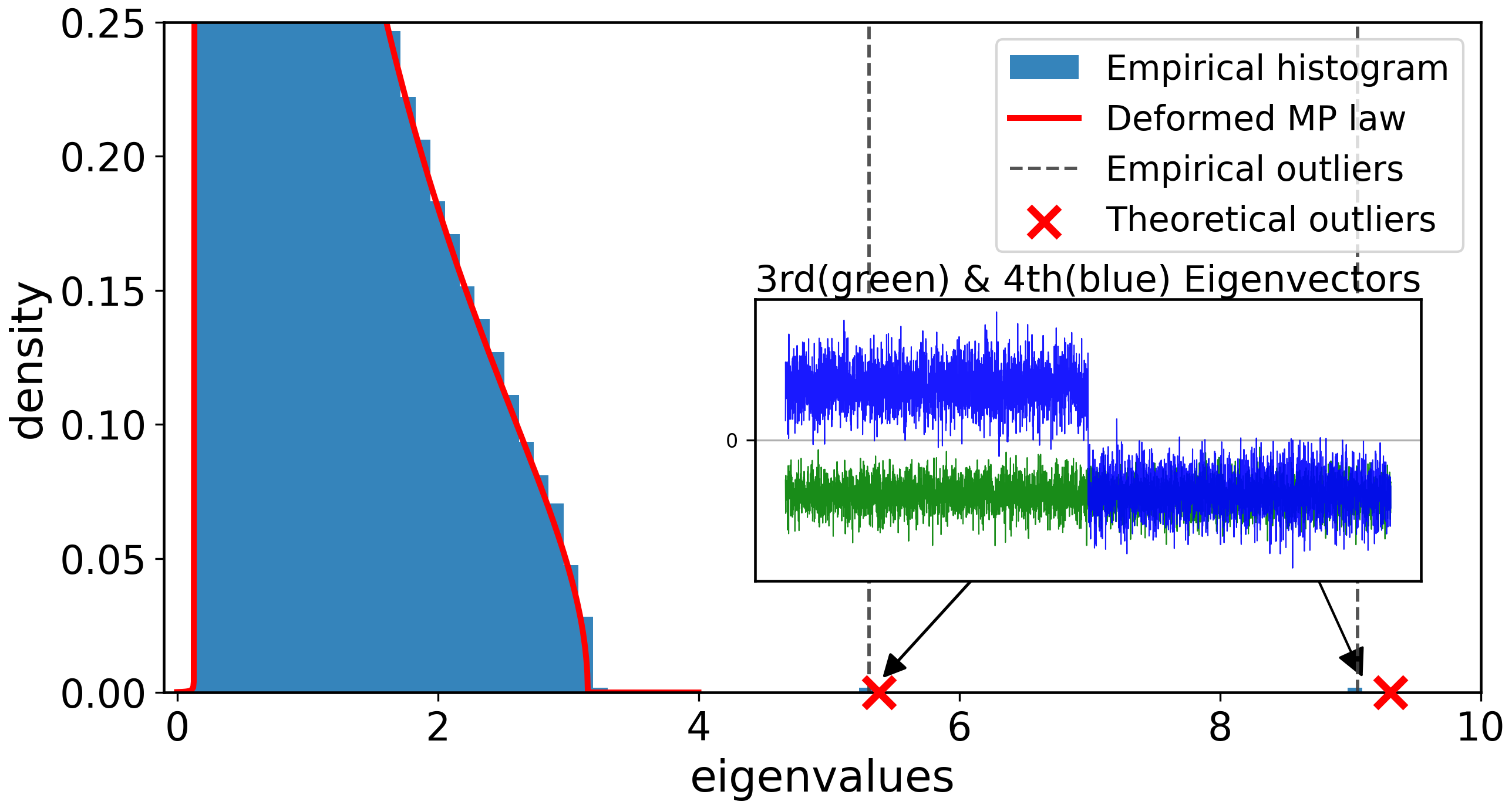
Figure 2: Large-SNR proportional regime: informative CK spikes recover the XOR labels. We consider the same setting as in Figure 1 only increasing SNR to r=352r=35^{2}. Left: spectrum of 𝑲\bm{K} (blue) together with the predicted curve from Theorem 5 (red curve). To focus on the order-one eigenvalues, we do not display the first two extremely large eigenvalues λ^1=153.9\widehat{\lambda}_{1}=153.9 and λ^2=153.1\widehat{\lambda}_{2}=153.1 predicted by (4.10). The red ×\color[rgb]{1,0,0}{\mathbf{\times}} are the theoretical locations of the order-one outliers. The subfigure presents the 3rd & 4th eigenvectors against sample index. The 4th outlier eigenvector of 𝑲\bm{K} is informative for linear classification of XOR. Right: kernel-PCA visualization using the 3rd & 4th PCs of 𝑲\bm{K}. In contrast to Figure 1, these two spectral coordinates clearly separate the positive and negative classes by a linear boundary.

Theorem 5 shows that increasing the SNR to r2=Θ​(n1/2)r^{2}=\Theta(n^{1/2}) can lead to the emergence of a label-informative order-one CK outlier. In this regime, the quadratic component of σ\sigma is no longer negligible when cσ≠0c_{\sigma}\neq 0, making linear spectral classification of XOR possible through (4.13) in Theorem 5(iv). When moving from Figure 1 to Figure 2, we only increase the SNR from 3636 to 12251225. This change produces two additional outliers, one of whose eigenvectors asymptotically aligns with the XOR labels 𝒚{\bm{y}}.

Figures 1 and 2 use the centered and normalized ReLU activation, for which both bσb_{\sigma} and cσc_{\sigma} are nonzero. In Figure 3, we show the same SNR-driven phase transition using a centered and normalized activation σ​(x)∝x2+1−1\sigma(x)\propto\sqrt{x^{2}+1}-1, for which bσ=0b_{\sigma}=0 and cσ≠0c_{\sigma}\neq 0. Since bσ=0b_{\sigma}=0, the diverging linear outliers predicted by Theorem 3(iii) and Theorem 5(ii) are absent. As the SNR increases from r2=36r^{2}=36 to 625625, the second eigenvector develops a two-class structure, and XOR becomes linearly classifiable using CK eigenvectors.

Refer to caption
Refer to caption
Refer to caption
Refer to caption
Figure 3: CK spectral phase transition driven by SNR. Top: CK spectrum in the finite-SNR regime with r=6r=6; no eigenvalue separates from the bulk. Bottom: CK spectrum in the large-SNR regime with r=25r=25. Two quadratic eigenvalues separate from the bulk, and the second leading eigenvector aligns with the XOR labels. Here the activation σ​(x)∝x2+1−1\sigma(x)\propto\sqrt{x^{2}+1}-1, n=5000n=5000, and N=d=15000N=d=15000.

6.2 Knob II: Activation Functions

Figures 1, 2, and 3 already show that changing the activation function can lead to qualitatively different CK spectral behavior. We now present two additional examples: the emergence of uninformative spikes and the absence of informative spikes.

Refer to caption
Refer to caption
Figure 4: Emergence of uninformative spikes when SNR=0\mathrm{SNR}=0. CK spectra under the activation function fαf_{\alpha} defined in (6.1), with n=6000n=6000, N=d=1000N=d=1000, and r=0r=0. Left: α=2\alpha=2. Right: α=1.5\alpha=1.5. Two uninformative spikes emerge and are close to the theoretical predictions from Theorem 3(ii), shown by red ×\color[rgb]{1,0,0}{\mathbf{\times}} markers.
Uninformative spikes can emerge even in the null model.

Theorem 3(ii) describes uninformative spikes of the CK matrix even when r=0r=0, namely for an isotropic Gaussian dataset. These uninformative spikes are caused by the nonzero quadratic coefficient cσ≠0c_{\sigma}\neq 0. Such spikes were studied by [BP22] for more general datasets, while our result gives a precise characterization of their locations for Gaussian data. To illustrate their emergence in the CK matrix, we consider the single-parameter family of activation functions from [BP22],

fα​(x)=cos⁡(α​x)−e−α2/2e−α2​(cosh⁡(α2)−1).f_{\alpha}(x)=\frac{\cos(\alpha x)-e^{-\alpha^{2}/2}}{\sqrt{e^{-\alpha^{2}}\bigl(\cosh(\alpha^{2})-1\bigr)}}. (6.1)

These functions satisfy Assumption 1. Moreover, bσ=0b_{\sigma}=0 for all choices of α\alpha, while cσc_{\sigma} varies with α\alpha. Figure 4 plots the CK spectra under fαf_{\alpha} in the null model SNR=0\mathrm{SNR}=0 for α=2\alpha=2 and α=1.5\alpha=1.5. As α\alpha decreases, two outlier spikes emerge in the CK spectrum. These two uninformative spikes arise from the population covariance of the CK and from the CK mean; Theorem 3(ii) predicts that their locations are asymptotically close.

XOR remains linearly nonseparable at large SNR when cσ=0c_{\sigma}=0.

If the activation function σ\sigma satisfies cσ=0c_{\sigma}=0, then the quadratic component in the CK is absent. As discussed in Theorem 5, this implies that the CK cannot be used to linearly classify XOR for any signal-to-noise ratio. Figure 5 follows the same setting as the bottom panel of Figure 3, changing only the activation to σ∝tanh\sigma\propto\tanh with cσ=0c_{\sigma}=0. Here SNR=625\mathrm{SNR}=625. By Theorem 5, only two diverging linear outliers separate from the bulk. Moreover, their associated spectral coordinates are not linearly separable with respect to the XOR labels.

Refer to caption
Refer to caption
Figure 5: Large-SNR regime with cσ=0c_{\sigma}=0: linear classification of XOR still fails. Here n=5000n=5000, N=d=15000N=d=15000, r=25r=25, and σ​(x)∝tanh⁡(x)\sigma(x)\propto\tanh(x), so cσ=0c_{\sigma}=0. Left: spectrum of 𝑲\bm{K} (blue), together with the theoretical locations of the two diverging outliers predicted by Theorem 5(ii), shown by red ×\color[rgb]{1,0,0}{\times} markers. The outlier eigenvectors, displayed in the inset, exhibit a four-block pattern associated with the four Gaussian-mixture components but remain asymptotically orthogonal to the XOR label vector 𝒚{\bm{y}}. Right: kernel-PCA visualization of 𝑲\bm{K}. Thus the leading nontrivial spectral coordinates are not linearly separable with respect to the XOR labels.

6.3 Knob III: Weight Structure

Following Theorem 6, we generate a rank-one perturbation of the randomly initialized weights, 𝑾1=𝑾+θ​𝒂​𝒃⊤\bm{W}_{1}=\bm{W}+\theta{\bm{a}}{\bm{b}}^{\top}, as a model of pretrained weights. In Figure 6, we plot the spectrum of the projected CK matrix 𝑲s\bm{K}_{s} and its PCs for the centered and normalized ReLU activation, an XOR dataset with SNR r2=36r^{2}=36, and spike strength θ=5\theta=5. The rank-one structure in the pretrained weights produces informative spikes. As predicted by Theorem 6, two order-one outlier eigenvalues emerge, and the second leading eigenvector exhibits a two-class structure that enables linear classification of XOR.

Refer to caption
Refer to caption
Figure 6: Spiked-weight regime: a weight-induced spike aligns with XOR labels. Here N=n=8000N=n=8000, d=4000d=4000, the SNR is r2=36r^{2}=36, σ​(x)∝ReLU​(x)\sigma(x)\propto\mathrm{ReLU}(x), and the weight spike strength in (4.14) is θ=5.0\theta=5.0. Left: spectrum of 𝑲s\bm{K}_{s} (blue), as defined in Theorem 6, together with the isolated eigenvalue locations predicted by Theorem 6, shown by red ×\color[rgb]{1,0,0}{\times} markers. The top two empirical eigenvectors are shown in the insets; the second one enables linear classification of XOR. Right: kernel-PCA visualization of the samples using the second and first PCs of 𝑲s\bm{K}_{s}.
Pretrained weights from feature learning on a real-world dataset.

The pretrained-weight model in (4.14), used in Theorem 6, is an idealized model for our analysis. We now show that real pretrained weights obtained during training can exhibit similar label-aligned CK spikes. A recent line of work [MM21, MM19, WES+23] has tracked the evolution of the empirical spectral distribution of weight matrices throughout the training process of deep NNs. We focus on an early-training phase in which the weight spectrum is well described by an “MP bulk++spikes” structure. The emergence of spikes in the weight spectrum is strongly related to feature learning in NNs [FCB22] and suggests that these spikes carry task-relevant information.

We consider the CK matrix formed using pretrained weights extracted from the first-layer weight matrix of a 20-layer fully connected NN trained on CIFAR-2. Each hidden layer has width N=512N=512, and the input dimension is d=3072d=3072. We focus on the first 50 steps of SGD training, using learning rate 0.050.05, momentum 0.50.5, and batch size 128128. At step 50, the test accuracy is 80.4%80.4\%, and the training accuracy is 91.41%91.41\%. Figure 7 shows the spectra of the first-layer trained weights at steps 11, 22, and 5050 (bottom row), together with the spectra of CK matrices evaluated on XOR data using these pretrained weights (top row). The emergence of spikes in the weight spectra during training suggests that the model is learning task-dependent features.

For the CK matrices in this experiment, n=8000n=8000, N=512N=512, d=3072d=3072, and the SNR is r2=36r^{2}=36. In contrast to the prediction of Theorem 3 for randomly initialized weights, the pretrained CK at step 50 exhibits four spikes. We omit the top outlier in Figure 7 because it is a large-order outlier. The fourth leading eigenvector aligns with the XOR labels. After sufficient training, this eigenvector transitions from pure noise to near-perfect alignment with the XOR labels, thereby enabling linear classification.

These experiments suggest that the LE approximation of the CK can break down even during the early stages of training. They also indicate that, under suitable training regimes and parameter choices, there can be a critical phase transition in which the emergence of weight spikes makes quadratic channels in the CK nonnegligible. One possible explanation is that training the NN induces spiked eigenvalues with eigenvectors that align with XOR labels, even though the model is not trained directly on the XOR task. Theorem 6 captures this mechanism through an idealized model in which a large spike is artificially introduced into the weights, producing a spiked CK eigenvalue with an XOR-label-aligned eigenvector.

Refer to caption
Refer to caption
Refer to caption
Refer to caption
Refer to caption
Refer to caption
Figure 7: Pretrained weights help linear classification of XOR. Top: CK spectra with pretrained weights at training steps 11, 22, and 5050. For these CK matrices, n=8000n=8000, N=512N=512, d=3072d=3072, the SNR is r2=36r^{2}=36, and σ​(x)∝ReLU​(x)\sigma(x)\propto\mathrm{ReLU}(x). Bottom: spectra of the first-layer weight matrix of a NN trained on CIFAR-2 at steps 11, 22, and 5050. The red curves show the MP laws.

6.4 Knob IV: Sample Size

Following Section 4.4, we study CK spectra under the quadratic sample-size scaling n=Θ​(d2)n=\Theta(d^{2}). Figure 8 shows the spectrum and PCs of the projected CK matrix for the centered and normalized ReLU activation and an XOR dataset with finite SNR r2=6.25r^{2}=6.25. Here n=15000n=15000, N=20000N=20000, and d=150d=150. In this scaling, many outliers emerge in the unprojected CK spectrum. We therefore focus on the projected CK matrix 𝑲σ\bm{K}_{\sigma} defined in Theorem 7, which isolates the label-aligned spike. We observe a single eigenvalue outside the bulk of the deformed MP law μq\mu_{\rm q}, and its eigenvector aligns with the XOR labels 𝒚{\bm{y}}, even at an SNR smaller than that used in Figure 1.

Refer to caption
Refer to caption
Figure 8: Quadratic sample-size regime: an informative CK spike aligns with XOR labels. Here n=15000n=15000, N=20000N=20000, d=150d=150, the SNR is r2=6.25r^{2}=6.25, and σ​(x)∝ReLU​(x)\sigma(x)\propto\mathrm{ReLU}(x). Left: spectrum of the projected CK matrix 𝑲σ\bm{K}_{\sigma}, defined in Theorem 7, together with the asymptotic spike prediction from Theorem 7, shown by a red ×\color[rgb]{1,0,0}{\times} marker. There is a single isolated spike, whose eigenvector is displayed in the inset. Its blockwise sign pattern aligns with the binary XOR partition, explaining the linear class separation seen on the right. Right: kernel-PCA visualization of the samples using the top two PCs of 𝑲σ\bm{K}_{\sigma}.

7 Conclusion

We introduce a quadratic equivalent framework and illustrate its use by characterizing when nonlinear structure becomes spectrally visible in the CK matrix. For the nonlinear XOR problem, we show that in the proportional limit with finite SNR, the CK can exhibit outliers, but their eigenvectors are asymptotically unaligned with labels. In contrast, increasing SNR, moving to the quadratic sample-size regime, or adding pretrained structure to the weights can make the quadratic feature non-negligible and produce informative outliers that enable linear spectral classification. Our results highlight the complex and subtle relationship between common ML training “knobs” and the emergence of spikes in the spectrum of ML models. Extending QE to more general scalings, deeper networks, and other forms of structured data is an interesting direction.

Acknowledgments

CC and TK were supported in part by NSF grant DMS-2400246. ZW and MWM would like to acknowledge the NSF and the DARPA DIAL and DARPA AIQ programs for partial support of this work.

References

  • [AS64] M. Abramowitz and I. A. Stegun (1964) Handbook of mathematical functions with formulas, graphs, and mathematical tables. Vol. 55, US Government printing office. Cited by: §A.2.
  • [AP20] B. Adlam and J. Pennington (2020) The neural tangent kernel in high dimensions: triple descent and a multi-scale theory of generalization. In International Conference on Machine Learning, pp. 74–84. Cited by: §1, §1, §2.
  • [BES+22] J. Ba, M. A. Erdogdu, T. Suzuki, Z. Wang, D. Wu, and G. Yang (2022) High-dimensional asymptotics of feature learning: how one gradient step improves the representation. arXiv preprint arXiv:2205.01445. Cited by: §1, §1, §4.3, §4.3.
  • [BES+23] J. Ba, M. A. Erdogdu, T. Suzuki, Z. Wang, and D. Wu (2023) Learning in the presence of low-dimensional structure: a spiked random matrix perspective. In Thirty-seventh Conference on Neural Information Processing Systems (NeurIPS 2023), Cited by: §1, §2, §4.3.
  • [BS98] Z. Bai and J. W. Silverstein (1998) No eigenvalues outside the support of the limiting spectral distribution of large-dimensional sample covariance matrices. The Annals of Probability 26 (1), pp. 316–345. Cited by: §C.2.
  • [BS10] Z. Bai and J. W. Silverstein (2010) Spectral analysis of large dimensional random matrices. Vol. 20, Springer. Cited by: §3, §3.
  • [BAP05] J. Baik, G. B. Arous, and S. Péché (2005) Phase transition of the largest eigenvalue for nonnull complex sample covariance matrices. The Annals of Probability 33 (5), pp. 1643–1697. Cited by: §1, §2.
  • [BN03] M. Belkin and P. Niyogi (2003) Laplacian eigenmaps for dimensionality reduction and data representation. Neural Computation 15 (6), pp. 1373–1396. External Links: Document Cited by: §1.
  • [BPQ+24] N. Belrose, Q. Pope, L. Quirke, A. Mallen, and X. Fern (2024) Neural networks learn statistics of increasing complexity. arXiv preprint arXiv:2402.04362. Cited by: §2.
  • [BN12] F. Benaych-Georges and R. R. Nadakuditi (2012) The singular values and vectors of low rank perturbations of large rectangular random matrices. Journal of Multivariate Analysis 111, pp. 120–135. Cited by: §G.3, §G.3, Remark, Remark.
  • [BP21] L. Benigni and S. Péché (2021) Eigenvalue distribution of some nonlinear models of random matrices. Electronic Journal of Probability 26, pp. 1–37. Cited by: §3.
  • [BP22] L. Benigni and S. Péché (2022) Largest eigenvalues of the conjugate kernel of single-layered neural networks. arXiv preprint arXiv:2201.04753. Cited by: Appendix C, §1.1, §2, §4.1, §6.2.
  • [BEK+14] A. Bloemendal, L. Erdős, A. Knowles, H. Yau, and J. Yin (2014) Isotropic local laws for sample covariance and generalized Wigner matrices. Electronic Journal of Probability 19 (none), pp. 1 – 53. External Links: Document Cited by: §C.2, §C.4.3.
  • [BM24] S. Bombari and M. Mondelli (2024-21–27 Jul) How spurious features are memorized: precise analysis for random and NTK features. In Proceedings of the 41st International Conference on Machine Learning, R. Salakhutdinov, Z. Kolter, K. Heller, A. Weller, N. Oliver, J. Scarlett, and F. Berkenkamp (Eds.), Proceedings of Machine Learning Research, Vol. 235, pp. 4267–4299. External Links: Link Cited by: §2.
  • [BPH23] D. Bosch, A. Panahi, and B. Hassibi (2023) Precise asymptotic analysis of deep random feature models. In The Thirty Sixth Annual Conference on Learning Theory, pp. 4132–4179. Cited by: §1.1.
  • [CM24] C. Cheng and A. Montanari (2024) Dimension free ridge regression. The Annals of Statistics 52 (6), pp. 2879–2912. Cited by: §2.
  • [CS13] X. Cheng and A. Singer (2013) The spectrum of random inner-product kernel matrices. Random Matrices: Theory and Applications 2 (04), pp. 1350010. Cited by: §G.2.2, §2.
  • [CL06] R. R. Coifman and S. Lafon (2006) Diffusion maps. Applied and Computational Harmonic Analysis 21 (1), pp. 5–30. External Links: Document Cited by: §1.
  • [CB16] R. Couillet and F. Benaych-Georges (2016) Kernel spectral clustering of large dimensional data. Electronic Journal of Statistics 10 (1), pp. 1393 – 1454. External Links: Document, Link Cited by: Appendix D, Appendix D, Appendix D, Appendix D, Appendix D, §4.1.
  • [COU19] R. Couillet (2019) High dimensional robust classification: a random matrix analysis. In 2019 IEEE 8th International Workshop on Computational Advances in Multi-Sensor Adaptive Processing (CAMSAP), pp. 420–424. Cited by: §2.
  • [DM24] I. Dabo and C. Male (2024) A traffic approach for profiled pennington-worah matrices. arXiv preprint arXiv:2409.13433. Cited by: §2.
  • [DLS22] A. Damian, J. Lee, and M. Soltanolkotabi (2022) Neural networks can learn representations with gradient descent. In Conference on Learning Theory, pp. 5413–5452. Cited by: §1.
  • [DPC+24] Y. Dandi, L. Pesce, H. Cui, F. Krzakala, Y. M. Lu, and B. Loureiro (2024) A random matrix theory perspective on the spectrum of learned features and asymptotic generalization capabilities. arXiv preprint arXiv:2410.18938. Cited by: §1.
  • [DK70] C. Davis and W. M. Kahan (1970) The rotation of eigenvectors by a perturbation. iii. SIAM Journal on Numerical Analysis 7 (1), pp. 1–46. Cited by: §C.4.
  • [DD25] S. Demir and Z. Dogan (2025) Asymptotic analysis of two-layer neural networks after one gradient step under gaussian mixtures data with structure. In International Conference on Learning Representations, External Links: Link, 2503.00856 Cited by: §2, §4.3, §4.3.
  • [26] NIST Digital Library of Mathematical Functions. Note: https://dlmf.nist.gov/, Release 1.2.4 of 2025-03-15F. W. J. Olver, A. B. Olde Daalhuis, D. W. Lozier, B. I. Schneider, R. F. Boisvert, C. W. Clark, B. R. Miller, B. V. Saunders, H. S. Cohl, and M. A. McClain, eds. External Links: Link Cited by: §A.2, §A.2, §A.2.
  • [DV13] Y. Do and V. Vu (2013) The spectrum of random kernel matrices: universality results for rough and varying kernels. Random Matrices: Theory and Applications 2 (03), pp. 1350005. Cited by: §2.
  • [EL 10] N. El Karoui (2010) The spectrum of kernel random matrices. The Annals of Statistics 38 (1), pp. 1–50. Cited by: §C.1, §2.
  • [EKY13] L. Erdős, A. Knowles, and H. Yau (2013) Averaging fluctuations in resolvents of random band matrices. In Annales Henri Poincaré, Vol. 14, pp. 1837–1926. Cited by: Appendix A.
  • [FMP+26] Z. Fan, R. Ma, E. Paquette, and Z. Wang (2026) Anisotropic local law for non-separable sample covariance matrices. arXiv preprint arXiv:2602.17960. Cited by: §C.4.3, §C.4.4, §G.3.
  • [FW20] Z. Fan and Z. Wang (2020) Spectra of the conjugate kernel and neural tangent kernel for linear-width neural networks. Advances in neural information processing systems 33, pp. 7710–7721. Cited by: §A.1, §A.1, §2, §3, §3.
  • [FEL23] M. J. Feldman (2023) Spectral properties of elementwise-transformed spiked matrices. arXiv preprint arXiv:2311.02040. Cited by: §1, §2.
  • [FCB22] S. Frei, N. S. Chatterji, and P. L. Bartlett (2022) Random feature amplification: feature learning and generalization in neural networks. arXiv preprint arXiv:2202.07626. Cited by: §6.3.
  • [GKX19a] B. Ghorbani, S. Krishnan, and Y. Xiao (2019) An investigation into neural net optimization via hessian eigenvalue density. In Proceedings of the 36th International Conference on Machine Learning, K. Chaudhuri and R. Salakhutdinov (Eds.), Proceedings of Machine Learning Research, Vol. 97, pp. 2232–2241. External Links: Link Cited by: §1.
  • [GMM+19b] B. Ghorbani, S. Mei, T. Misiakiewicz, and A. Montanari (2019) Limitations of lazy training of two-layers neural network. Advances in Neural Information Processing Systems 32. Cited by: §2.
  • [GLA23] M. Glasgow (2023) Sgd finds then tunes features in two-layer neural networks with near-optimal sample complexity: a case study in the xor problem. arXiv preprint arXiv:2309.15111. Cited by: §2.
  • [GLR+21] S. Goldt, B. Loureiro, G. Reeves, F. Krzakala, M. Mézard, and L. Zdeborová (2021) The gaussian equivalence of generative models for learning with shallow neural networks. Proceedings of Machine Learning Research vol 145, pp. 1–46. Cited by: §1.1.
  • [GSS21] F. Götze, H. Sambale, and A. Sinulis (2021) Concentration inequalities for polynomials in α\alpha-sub-exponential random variables. Electronic Journal of Probability 26 (none), pp. 1 – 22. External Links: Document, Link Cited by: §E.2.
  • [GDZ+22] L. Gu, Y. Du, Y. Zhang, D. Xie, S. Pu, R. C. Qiu, and Z. Liao (2022) ”Lossless” compression of deep neural networks: a high-dimensional neural tangent kernel approach. In Advances in Neural Information Processing Systems, A. H. Oh, A. Agarwal, D. Belgrave, and K. Cho (Eds.), External Links: Link Cited by: §2.
  • [GKK+23] A. Guionnet, J. Ko, F. Krzakala, P. Mergny, and L. Zdeborová (2023) Spectral phase transitions in non-linear wigner spiked models. arXiv preprint arXiv:2310.14055. Cited by: §2.
  • [GP26] A. Guionnet and V. Piccolo (2026) Global law of conjugate kernel random matrices with heavy-tailed weights. Electronic Journal of Probability 31, pp. 1–58. Cited by: §2.
  • [HG16] D. Hendrycks and K. Gimpel (2016) Gaussian error linear units (gelus). arXiv preprint arXiv:1606.08415. Cited by: §A.4.
  • [HSW+21] E. J. Hu, Y. Shen, P. Wallis, Z. Allen-Zhu, Y. Li, S. Wang, L. Wang, and W. Chen (2021) Lora: low-rank adaptation of large language models. arxiv 2021. arXiv preprint arXiv:2106.09685 10. Cited by: §4.3.
  • [HL22] H. Hu and Y. M. Lu (2022) Universality laws for high-dimensional learning with random features. IEEE Transactions on Information Theory 69 (3), pp. 1932–1964. Cited by: §1.1, §1.
  • [HMZ+23] M. Huh, H. Mobahi, R. Zhang, B. Cheung, P. Agrawal, and P. Isola (2023) The low-rank simplicity bias in deep networks. Transactions on Machine Learning Research. Note: External Links: ISSN 2835-8856, Link Cited by: §2.
  • [JGH18] A. Jacot, F. Gabriel, and C. Hongler (2018) Neural tangent kernel: convergence and generalization in neural networks. In Advances in neural information processing systems, pp. 8571–8580. Cited by: §1, §1.
  • [JL09] I. M. Johnstone and A. Y. Lu (2009) On consistency and sparsity for principal components analysis in high dimensions. Journal of the American Statistical Association 104 (486), pp. 682–693. External Links: Document Cited by: §1.
  • [JOL02] I. T. Jolliffe (2002) Principal component analysis. 2 edition, Springer Series in Statistics, Springer, New York. External Links: Document Cited by: §1.
  • [KY17] A. Knowles and J. Yin (2017) Anisotropic local laws for random matrices. Probability Theory and Related Fields 169, pp. 257–352. Cited by: §C.4.3, §C.4.3, §G.3.
  • [LM00] B. Laurent and P. Massart (2000) Adaptive estimation of a quadratic functional by model selection. Annals of statistics, pp. 1302–1338. Cited by: §A.1.
  • [LHY25] X. Li, X. Han, and Q. Yang (2025) Eigen analysis of conjugate kernel and neural tangent kernel. In Forty-second International Conference on Machine Learning, Cited by: §2.
  • [LCM20] Z. Liao, R. Couillet, and M. W. Mahoney (2020) A random matrix analysis of random fourier features: beyond the gaussian kernel, a precise phase transition, and the corresponding double descent. Advances in Neural Information Processing Systems 33, pp. 13939–13950. Cited by: §1.
  • [LC19] Z. Liao and R. Couillet (2019-12) On inner-product kernels of high dimensional data. 2019 IEEE 8th International Workshop on Computational Advances in Multi-Sensor Adaptive Processing (CAMSAP), pp. 579–583. External Links: Document Cited by: §2.
  • [LM21] Z. Liao and M. W. Mahoney (2021) Hessian eigenspectra of more realistic nonlinear models. Advances in Neural Information Processing Systems 34, pp. 20104–20117. Cited by: §1.
  • [LM25] Z. Liao and M. W. Mahoney (2025) Random matrix theory for deep learning: beyond eigenvalues of linear models. arXiv preprint arXiv:2506.13139. Cited by: §1.
  • [LLC18] C. Louart, Z. Liao, and R. Couillet (2018) A random matrix approach to neural networks. The Annals of Applied Probability 28 (2), pp. 1190–1248. Cited by: §3.
  • [LY25] Y. M. Lu and H. Yau (2025) An equivalence principle for the spectrum of random inner-product kernel matrices with polynomial scalings. The Annals of Applied Probability 35 (4), pp. 2411–2470. Cited by: §G.2.1, §G.2.1, §G.2.2, §G.2.2, §2, Lemma 65, Lemma 67.
  • [MP67] V. A. Marčenko and L. A. Pastur (1967) Distribution of eigenvalues for some sets of random matrices. Mathematics of the USSR-Sbornik 1 (4), pp. 457–483. Cited by: §3.
  • [MM19] C. H. Martin and M. W. Mahoney (2019) Traditional and heavy-tailed self regularization in neural network models. In Proceedings of the 36th International Conference on Machine Learning, pp. 4284–4293. Cited by: §1, §4.3, §6.3.
  • [MM20] C. H. Martin and M. W. Mahoney (2020) Heavy-tailed Universality predicts trends in test accuracies for very large pre-trained deep neural networks. In Proceedings of the 20th SIAM International Conference on Data Mining, pp. . Cited by: §1, §4.3.
  • [MM21] C. H. Martin and M. W. Mahoney (2021) Implicit self-regularization in deep neural networks: evidence from random matrix theory and implications for learning. Journal of Machine Learning Research 22 (165), pp. 1–73. Cited by: §1, §4.3, §6.3.
  • [MPM21] C. H. Martin, T. S. Peng, and M. W. Mahoney (2021) Predicting trends in the quality of state-of-the-art neural networks without access to training or testing data. Nature Communications 12 (4122), pp. 1–13. Cited by: §1, §4.3.
  • [MM22] S. Mei and A. Montanari (2022) The generalization error of random features regression: precise asymptotics and the double descent curve. Communications on Pure and Applied Mathematics 75 (4), pp. 667–766. Cited by: §1.1, §1, §2.
  • [MS24] T. Misiakiewicz and B. Saeed (2024) A non-asymptotic theory of kernel ridge regression: deterministic equivalents, test error, and gcv estimator. arXiv preprint arXiv:2403.08938. Cited by: §2.
  • [MLH+23] B. Moniri, D. Lee, H. Hassani, and E. Dobriban (2023) A theory of non-linear feature learning with one gradient step in two-layer neural networks. arXiv preprint arXiv:2310.07891. Cited by: §1.
  • [NAD08] B. Nadler (2008-12) Finite sample approximation results for principal component analysis: a matrix perturbation approach. The Annals of Statistics 36 (6), pp. 2791–2817. External Links: Document Cited by: §1.
  • [NJW01] A. Ng, M. Jordan, and Y. Weiss (2001) On spectral clustering: analysis and an algorithm. In Advances in Neural Information Processing Systems, T. Dietterich, S. Becker, and Z. Ghahramani (Eds.), Vol. 14, pp. . External Links: Link Cited by: §4.1.
  • [NPR10] I. Nourdin, G. Peccati, and G. Reinert (2010) Invariance principles for homogeneous sums: Universality of Gaussian Wiener chaos. The Annals of Probability 38 (5), pp. 1947 – 1985. External Links: Document, Link Cited by: §G.1.
  • [PWZ24] P. Pandit, Z. Wang, and Y. Zhu (2024) Universality of kernel random matrices and kernel regression in the quadratic regime. arXiv preprint arXiv:2408.01062. External Links: 2408.01062, Link Cited by: §G.2.2, §2.
  • [PÉC06] S. Péché (2006) The largest eigenvalue of small rank perturbations of hermitian random matrices. Probability Theory and Related Fields 134 (1), pp. 127–173. Cited by: §2.
  • [PÉC19] S. Péché (2019) A note on the pennington-worah distribution. Electronic Communications in Probability 24, pp. 1–7. Cited by: §2.
  • [PW17] J. Pennington and P. Worah (2017) Nonlinear random matrix theory for deep learning. In Advances in Neural Information Processing Systems, pp. 2637–2646. Cited by: §1, §1, §2, §3.
  • [RGK+21] M. Refinetti, S. Goldt, F. Krzakala, and L. Zdeborová (2021) Classifying high-dimensional gaussian mixtures: where kernel methods fail and neural networks succeed. In International Conference on Machine Learning, pp. 8936–8947. Cited by: §1, §2, §2.
  • [RGL+24] R. Rende, F. Gerace, A. Laio, and S. Goldt (2024) A distributional simplicity bias in the learning dynamics of transformers. Advances in Neural Information Processing Systems 37, pp. 96207–96228. Cited by: §2.
  • [ROS70] H. P. Rosenthal (1970) On the subspaces of l p (p¿ 2) spanned by sequences of independent random variables. Israel Journal of Mathematics 8 (3), pp. 273–303. Cited by: §A.1.
  • [RS00] S. T. Roweis and L. K. Saul (2000) Nonlinear dimensionality reduction by locally linear embedding. Science 290 (5500), pp. 2323–2326. External Links: Document Cited by: §1.
  • [SBL16] L. Sagun, L. Bottou, and Y. LeCun (2016) Singularity of the hessian in deep learning. CoRR abs/1611.07476. External Links: Link, 1611.07476 Cited by: §1.
  • [SSM98] B. Schölkopf, A. Smola, and K. Müller (1998) Nonlinear component analysis as a kernel eigenvalue problem. Neural Computation 10 (5), pp. 1299–1319. External Links: Document Cited by: §1.
  • [SC95] J. W. Silverstein and S. Choi (1995) Analysis of the limiting spectral distribution of large dimensional random matrices. Journal of Multivariate Analysis 54 (2), pp. 295–309. Cited by: §A.3.
  • [TGM25] H. Taheri, A. Ghosh, and A. Mazumdar (2025) On the theory of continual learning with gradient descent for neural networks. arXiv preprint arXiv:2510.05573. Cited by: §2.
  • [TdL00] J. B. Tenenbaum, V. de Silva, and J. C. Langford (2000) A global geometric framework for nonlinear dimensionality reduction. Science 290 (5500), pp. 2319–2323. External Links: Document Cited by: §1.
  • [TEo51] F. G. Tricomi, A. Erdélyi, et al. (1951) The asymptotic expansion of a ratio of gamma functions. Pacific J. Math 1 (1), pp. 133–142. Cited by: §A.2.
  • [VER12] R. Vershynin (2012) How close is the sample covariance matrix to the actual covariance matrix?. Journal of Theoretical Probability 25 (3), pp. 655–686. Cited by: §G.1.
  • [VER18] R. Vershynin (2018) High-dimensional probability: an introduction with applications in data science. Vol. 47, Cambridge University Press. Cited by: §A.2, §A.2, §A.2, §C.4.2.
  • [WES+23] Z. Wang, A. W. Engel, A. Sarwate, I. Dumitriu, and T. Chiang (2023) Spectral evolution and invariance in linear-width neural networks. In Thirty-seventh Conference on Neural Information Processing Systems, External Links: Link Cited by: §1, §6.3.
  • [WWF24] Z. Wang, D. Wu, and Z. Fan (2024) Nonlinear spiked covariance matrices and signal propagation in deep neural networks. In The Thirty Seventh Annual Conference on Learning Theory, pp. 4891–4957. Cited by: §C.3, §C.3, §C.4.3, §C.4.3, Appendix C, §G.4, §G.4, §1, §2, §3, §4.1.
  • [WZ24] Z. Wang and Y. Zhu (2024) Deformed semicircle law and concentration of nonlinear random matrices for ultra-wide neural networks. The Annals of Applied Probability 34 (2), pp. 1896–1947. Cited by: §C.1, §C.3, §G.2.2, §G.2, §1, §2.
  • [WED72] P. Wedin (1972) Perturbation bounds in connection with singular value decomposition. BIT Numerical Mathematics 12 (1), pp. 99–111. Cited by: §C.4.
  • [WHL+25] G. G. Wen, H. Hu, Y. M. Lu, Z. Fan, and T. Misiakiewicz (2025) When does gaussian equivalence fail and how to fix it: non-universal behavior of random features with quadratic scaling. arXiv preprint arXiv:2512.03325. Cited by: §2, §4.4.
  • [WIL25] A. G. Wilson (2025) Position: deep learning is not so mysterious or different. In Forty-second International Conference on Machine Learning Position Paper Track, External Links: Link Cited by: §2.
  • [XHM+22] L. Xiao, H. Hu, T. Misiakiewicz, Y. Lu, and J. Pennington (2022) Precise learning curves and higher-order scalings for dot-product kernel regression. Advances in Neural Information Processing Systems 35, pp. 4558–4570. Cited by: §2, §4.4.
  • [YTH+22] Y. Yang, R. Theisen, L. Hodgkinson, J. E. Gonzalez, K. Ramchandran, C. H. Martin, and M. W. Mahoney (2022) Test accuracy vs. generalization gap: model selection in nlp without accessing training or testing data (evaluating natural language processing models with generalization metrics that do not need access to any training or testing data). arXiv preprint arXiv:2202.02842. Cited by: §1, §4.3.

Contents

Appendix A Preliminaries

Throughout this paper, we utilize the stochastic domination notation introduced by [EKY13].

Definition 9 (Stochastic domination).

Consider two families of random variables

X={Xn​(u):n∈ℕ,u∈Un},Y={Yn​(u):n∈ℕ,u∈Un},X=\{X_{n}(u):n\in\mathbb{N},u\in U_{n}\},\,\,Y=\{Y_{n}(u):n\in\mathbb{N},u\in U_{n}\},

with parameter u∈Unu\in U_{n} where UnU_{n} is a possibly nn-dependent deterministic set. Let ℰ={En}n∈ℕ\mathcal{E}=\{E_{n}\}_{n\in\mathbb{N}} be a sequence of measure subsets, where each EnE_{n} is related to Xn​(u)X_{n}(u) and Yn​(u)Y_{n}(u).

  1. 1.

    We denote |X|≺Y|X|\prec Y or X=O≺(Y)X=O_{\prec}\mathopen{}\mathclose{{\left(Y}}\right) as the stochastic domination of XX by YY uniformly in u∈Unu\in U_{n}: if for all small ϵ>0\epsilon>0 and large D>0D>0, there exists some N0​(ϵ,D)N_{0}(\epsilon,D), such that for all n≥N0​(ϵ,D)n\geq N_{0}(\epsilon,D),

    supu∈Unℙ(|Xn(u)|≥nϵYn(u))≤n−D.\sup_{u\in U_{n}}\mathbb{P}\mathopen{}\mathclose{{\left(|X_{n}(u)|\geq n^{\epsilon}Y_{n}(u)}}\right)\leq n^{-D}.
  2. 2.

    For a family of random matrices 𝑨\bm{A} and a family of non-negative random variables ζ\zeta, 𝑨=O≺(ζ)\bm{A}=O_{\prec}\mathopen{}\mathclose{{\left(\zeta}}\right) represents |⟨𝒗,𝑨𝒖⟩|≺ζ∥𝒗∥∥𝒖∥|\langle{\bm{v}},\bm{A}{\bm{u}}\rangle|\prec\zeta\mathopen{}\mathclose{{\left\|{{\bm{v}}}}}\right\|\mathopen{}\mathclose{{\left\|{{\bm{u}}}}}\right\| uniformly for all deterministic vectors 𝒗{\bm{v}} and 𝒖{\bm{u}}.

If {𝑨n}\{\bm{A}_{n}\} are random matrices, we interpret ‖𝑨n‖op=oℙ​(1)\|\bm{A}_{n}\|_{\mathrm{op}}=o_{\mathbb{P}}(1) if and only if ‖𝑨n‖op→ℙ0.\|\bm{A}_{n}\|_{\mathrm{op}}\xrightarrow{\mathbb{P}}0. For simplicity, in the proofs, we use ‖𝑨n‖\|\bm{A}_{n}\| to represent operator norm ‖𝑨n‖op\|\bm{A}_{n}\|_{\mathrm{op}}.

A.1 Properties of XOR Data

We introduce the following notion of (τn,B)(\tau_{n},B)-orthonormality from [FW20].

Definition 10.

A matrix 𝑿∈ℝd×n\bm{X}\in\mathbb{R}^{d\times n} is (τn,B)(\tau_{n},B)-orthonormal if the columns {𝒙α}α=1n\{{\bm{x}}_{\alpha}\}_{\alpha=1}^{n} of 𝑿\bm{X} satisfy

|‖𝒙α‖−1|≤τn,|‖𝒙β‖−1|≤τn,|𝒙α⊤​𝒙β|≤τn\bigl\lvert\|{\bm{x}}_{\alpha}\|-1\bigr\rvert\leq\tau_{n},\quad\bigl\lvert\|{\bm{x}}_{\beta}\|-1\bigr\rvert\leq\tau_{n},\quad\bigl\lvert{\bm{x}}_{\alpha}^{\top}{\bm{x}}_{\beta}\bigr\rvert\leq\tau_{n} (A.1)

for all pairs α≠β∈[n]\alpha\neq\beta\in[n], ∑α=1n(‖𝒙α‖−1)2≤B2\sum_{\alpha=1}^{n}\bigl(\|{\bm{x}}_{\alpha}\|-1\bigr)^{2}\leq B^{2} and ‖𝑿‖≤B.\|\bm{X}\|\leq B.

Lemma 11.

Let 𝐗∈ℝd×n\bm{X}\in\mathbb{R}^{d\times n} be the XOR data matrix defined in (3.4). Assume either

  1. (A1)

    n≍dn\asymp d and r=O​(n1/4)r=O(n^{1/4}),  or

  2. (A2)

    n=O​(d2)n=O(d^{2}) and r=O​(1)r=O(1).

Then there exist constants c,C>0c,C>0 such that with probability at least 1−n−c1-n^{-c}, 𝐗\bm{X} satisfies (A.1) with

τn=C​(log⁡nd+r2d).\tau_{n}\;=\;C\Big(\sqrt{\frac{\log n}{d}}+\frac{r^{2}}{d}\Big). (A.2)

Moreover, on the same event,

∑α=1n(‖𝒙α‖−1)2≤∑α=1n(‖𝒙α‖2−1)2≤C​(nd+n​r2d2+n​r4d2),\sum_{\alpha=1}^{n}\big(\|\bm{x}_{\alpha}\|-1\big)^{2}\;\leq\;\sum_{\alpha=1}^{n}\big(\|\bm{x}_{\alpha}\|^{2}-1\big)^{2}\;\leq\;C\Big(\frac{n}{d}+\frac{nr^{2}}{d^{2}}+\frac{nr^{4}}{d^{2}}\Big), (A.3)

and also ‖𝐗‖≤C​(1+(1+r)​nd).\|\bm{X}\|\leq C\Big(1+(1+r)\sqrt{\frac{n}{d}}\Big). In particular, in regime (A1) one may take τn=C​log⁡nn\tau_{n}=C\sqrt{\frac{\log n}{n}} and B=C​(1+r)B=C(1+r), and in regime (A2) one may take τn=C​log⁡nd\tau_{n}=C\sqrt{\frac{\log n}{d}} and B=C​ndB=C\sqrt{\frac{n}{d}} such that 𝐗\bm{X} is (τn,B)(\tau_{n},B)-orthonormal with probability at least 1−n−c1-n^{-c}.

Proof.  Recall that θSNR:=r​n2​d\theta_{\mathrm{SNR}}:=r\sqrt{\frac{n}{2d}}, and 𝒖1,𝒖2∈ℝd\bm{u}_{1},\bm{u}_{2}\in\mathbb{R}^{d} and 𝒗1,𝒗2∈ℝn\bm{v}_{1},\bm{v}_{2}\in\mathbb{R}^{n} are orthonormal vectors defined by (3.6). This proof is basically following the proof of Proposition 3.3 of [FW20]. Write the columns as 𝒙α=𝒛α+𝒎α\bm{x}_{\alpha}=\bm{z}_{\alpha}+\bm{m}_{\alpha}, where 𝒛α\bm{z}_{\alpha} is the α\alpha-th column of 𝒁\bm{Z} and 𝒎α\bm{m}_{\alpha} is the α\alpha-th column of 𝑴\bm{M}. Since 𝑴=θSNR​𝒖1​𝒗1⊤+θSNR​𝒖2​𝒗2⊤\bm{M}=\theta_{\mathrm{SNR}}\,\bm{u}_{1}\bm{v}_{1}^{\top}+\theta_{\mathrm{SNR}}\,\bm{u}_{2}\bm{v}_{2}^{\top} and supp​(𝒗1)∩supp​(𝒗2)=∅\mathrm{supp}(\bm{v}_{1})\cap\mathrm{supp}(\bm{v}_{2})=\emptyset, for each α\alpha exactly one of 𝒗1​[α],𝒗2​[α]\bm{v}_{1}[\alpha],\bm{v}_{2}[\alpha] is nonzero, and 𝒎α=θSNR​𝒖1​𝒗1​[α]\bm{m}_{\alpha}=\theta_{\mathrm{SNR}}\bm{u}_{1}\bm{v}_{1}[\alpha] or θSNR​𝒖2​𝒗2​[α].\theta_{\mathrm{SNR}}\bm{u}_{2}\bm{v}_{2}[\alpha]. Using |𝒗1​[α]|=|𝒗2​[α]|=2/n|\bm{v}_{1}[\alpha]|=|\bm{v}_{2}[\alpha]|=\sqrt{2/n} on the support, we obtain for all α\alpha

‖𝒎α‖=θSNR​2n=r​n2​d​2n=rd,‖𝒎α‖2=r2d,‖𝒎α‖4=r4d2.\|\bm{m}_{\alpha}\|=\theta_{\mathrm{SNR}}\sqrt{\frac{2}{n}}=r\sqrt{\frac{n}{2d}}\sqrt{\frac{2}{n}}=\frac{r}{\sqrt{d}},\qquad\|\bm{m}_{\alpha}\|^{2}=\frac{r^{2}}{d},\qquad\|\bm{m}_{\alpha}\|^{4}=\frac{r^{4}}{d^{2}}. (A.4)

Now we verify the four requirements in the (τn,B)(\tau_{n},B)-orthonormal definition:

Uniform control of column norms.

For each α∈[n]\alpha\in[n],

‖𝒙α‖2=‖𝒛α‖2+2​𝒛α⊤​𝒎α+‖𝒎α‖2.\|\bm{x}_{\alpha}\|^{2}=\|\bm{z}_{\alpha}\|^{2}+2\,\bm{z}_{\alpha}^{\top}\bm{m}_{\alpha}+\|\bm{m}_{\alpha}\|^{2}. (A.5)

Since 𝒛α∼𝒩​(𝟎,𝑰d/d)\bm{z}_{\alpha}\sim\mathcal{N}(\bm{0},\bm{I}_{d}/d), we have d​‖𝒛α‖2∼χd2d\|\bm{z}_{\alpha}\|^{2}\sim\chi_{d}^{2}. By Lemma 1 of [LM00],

ℙ​(|‖𝒛α‖2−1|≥2​td+2​td)≤2​e−t\mathbb{P}\Big(\big|\|\bm{z}_{\alpha}\|^{2}-1\big|\geq 2\sqrt{\tfrac{t}{d}}+2\tfrac{t}{d}\Big)\leq 2e^{-t} (A.6)

for all t>0t>0. Taking t=C0​log⁡nt=C_{0}\log n and union bounding over α∈[n]\alpha\in[n] yields: with probability at least 1−2​n⋅n−C01-2n\cdot n^{-C_{0}}, for C0C_{0} large enough,

maxα∈[n]⁡|‖𝒛α‖2−1|≤C​log⁡nd.\max_{\alpha\in[n]}\big|\|\bm{z}_{\alpha}\|^{2}-1\big|\;\leq\;C\sqrt{\frac{\log n}{d}}. (A.7)

In particular, on the same event, maxα⁡‖𝒛α‖2≤2\max_{\alpha}\|\bm{z}_{\alpha}\|^{2}\leq 2 for all large nn. Conditioning on 𝒎α\bm{m}_{\alpha}, 𝒛α⊤​𝒎α|𝒎α∼𝒩​(0,r2/d2),\bm{z}_{\alpha}^{\top}\bm{m}_{\alpha}\,\big|\,\bm{m}_{\alpha}\sim\mathcal{N}\Big(0,r^{2}/d^{2}\Big), using (A.4). Hence for t=C0​log⁡nt=C_{0}\log n,

ℙ​(|𝒛α⊤​𝒎α|≥rd​2​t)≤2​e−t.\mathbb{P}\Big(|\bm{z}_{\alpha}^{\top}\bm{m}_{\alpha}|\geq\frac{r}{d}\sqrt{2t}\Big)\leq 2e^{-t}.

A union bound over α∈[n]\alpha\in[n] yields: with probability at least 1−n−c1-n^{-c},

maxα∈[n]⁡|𝒛α⊤​𝒎α|≤C​r​log⁡nd.\max_{\alpha\in[n]}|\bm{z}_{\alpha}^{\top}\bm{m}_{\alpha}|\;\leq\;C\,\frac{r\sqrt{\log n}}{d}. (A.8)

Plugging (A.7), (A.8), and ‖𝒎α‖2=r2/d\|\bm{m}_{\alpha}\|^{2}=r^{2}/d into (A.5) gives, with probability at least 1−n−c1-n^{-c},

maxα∈[n]⁡|‖𝒙α‖2−1|≤C​(log⁡nd+r​log⁡nd+r2d).\max_{\alpha\in[n]}\big|\|\bm{x}_{\alpha}\|^{2}-1\big|\;\leq\;C\Big(\sqrt{\frac{\log n}{d}}+\frac{r\sqrt{\log n}}{d}+\frac{r^{2}}{d}\Big). (A.9)

We now simplify the RHS under regimes (A1) and (A2). In both regimes, for large nn, r​log⁡nd≤log⁡nd+r2d.\frac{r\sqrt{\log n}}{d}\leq\sqrt{\frac{\log n}{d}}+\frac{r^{2}}{d}. Therefore (A.9) implies

maxα∈[n]⁡|‖𝒙α‖2−1|≤C​(log⁡nd+r2d).\max_{\alpha\in[n]}\big|\|\bm{x}_{\alpha}\|^{2}-1\big|\;\leq\;C\Big(\sqrt{\frac{\log n}{d}}+\frac{r^{2}}{d}\Big). (A.10)

Finally, notice that

|‖𝒙α‖−1|=|‖𝒙α‖2−1|‖𝒙α‖+1≤|‖𝒙α‖2−1|,\big|\|\bm{x}_{\alpha}\|-1\big|=\frac{\big|\|\bm{x}_{\alpha}\|^{2}-1\big|}{\|\bm{x}_{\alpha}\|+1}\leq\big|\|\bm{x}_{\alpha}\|^{2}-1\big|, (A.11)

so (A.10) yields

maxα∈[n]⁡|‖𝒙α‖−1|≤C​(log⁡nd+r2d).\max_{\alpha\in[n]}\big|\|\bm{x}_{\alpha}\|-1\big|\;\leq\;C\Big(\sqrt{\frac{\log n}{d}}+\frac{r^{2}}{d}\Big). (A.12)

This verifies the column-norm part of (τn,B)(\tau_{n},B)-orthonormality with τn\tau_{n} as in (A.2).

Uniform control of pairwise inner products.

Fix α≠β∈[n]\alpha\neq\beta\in[n]. Expand

𝒙α⊤​𝒙β=𝒛α⊤​𝒛β+𝒛α⊤​𝒎β+𝒎α⊤​𝒛β+𝒎α⊤​𝒎β.\bm{x}_{\alpha}^{\top}\bm{x}_{\beta}=\bm{z}_{\alpha}^{\top}\bm{z}_{\beta}+\bm{z}_{\alpha}^{\top}\bm{m}_{\beta}+\bm{m}_{\alpha}^{\top}\bm{z}_{\beta}+\bm{m}_{\alpha}^{\top}\bm{m}_{\beta}. (A.13)

The scalar 𝒛α⊤​𝒛β\bm{z}_{\alpha}^{\top}\bm{z}_{\beta} is not exactly Gaussian, but it is conditionally Gaussian: conditioning on 𝒛α\bm{z}_{\alpha}, 𝒛α⊤​𝒛β|𝒛α∼𝒩​(0,‖𝒛α‖2/d).\bm{z}_{\alpha}^{\top}\bm{z}_{\beta}\,\big|\,\bm{z}_{\alpha}\sim\mathcal{N}(0,\|\bm{z}_{\alpha}\|^{2}/d). On the event maxα⁡‖𝒛α‖2≤2\max_{\alpha}\|\bm{z}_{\alpha}\|^{2}\leq 2 we have

ℙ​(|𝒛α⊤​𝒛β|≥t|𝒛α)≤2​exp⁡(−d​t24​‖𝒛α‖2)≤2​exp⁡(−c​d​t2).\mathbb{P}\Big(|\bm{z}_{\alpha}^{\top}\bm{z}_{\beta}|\geq t\ \Big|\ \bm{z}_{\alpha}\Big)\leq 2\exp\Big(-\frac{dt^{2}}{4\|\bm{z}_{\alpha}\|^{2}}\Big)\leq 2\exp\Big(-c\,dt^{2}\Big).

Taking t=C​log⁡ndt=C\sqrt{\frac{\log n}{d}} and union bounding over all α≠β∈[n]\alpha\neq\beta\in[n] yields with probability at least 1−n−c1-n^{-c},

maxα≠β⁡|𝒛α⊤​𝒛β|≤C​log⁡nd.\max_{\alpha\neq\beta}|\bm{z}_{\alpha}^{\top}\bm{z}_{\beta}|\;\leq\;C\sqrt{\frac{\log n}{d}}. (A.14)

For α≠β\alpha\neq\beta, conditional on 𝒎β\bm{m}_{\beta}, 𝒛α⊤​𝒎β∼𝒩​(0,r2/d2),\bm{z}_{\alpha}^{\top}\bm{m}_{\beta}\sim\mathcal{N}\!(0,r^{2}/d^{2}), and similarly 𝒎α⊤​𝒛β∼𝒩​(0,r2/d2)\bm{m}_{\alpha}^{\top}\bm{z}_{\beta}\sim\mathcal{N}(0,r^{2}/d^{2}). A union bound over all α≠β\alpha\neq\beta gives, with probability at least 1−n−c1-n^{-c},

maxα≠β⁡|𝒛α⊤​𝒎β|≤C​r​log⁡nd,maxα≠β⁡|𝒎α⊤​𝒛β|≤C​r​log⁡nd.\max_{\alpha\neq\beta}|\bm{z}_{\alpha}^{\top}\bm{m}_{\beta}|\;\leq\;C\,\frac{r\sqrt{\log n}}{d},\qquad\max_{\alpha\neq\beta}|\bm{m}_{\alpha}^{\top}\bm{z}_{\beta}|\;\leq\;C\,\frac{r\sqrt{\log n}}{d}. (A.15)

Each 𝒎α\bm{m}_{\alpha} equals ±rd​𝒖1\pm\frac{r}{\sqrt{d}}\bm{u}_{1} or ±rd​𝒖2\pm\frac{r}{\sqrt{d}}\bm{u}_{2}. By Cauchy–Schwarz inequality, |𝒎α⊤​𝒎β|≤‖𝒎α‖​‖𝒎β‖=r2/d.|\bm{m}_{\alpha}^{\top}\bm{m}_{\beta}|\leq\|\bm{m}_{\alpha}\|\|\bm{m}_{\beta}\|=r^{2}/d. Hence

maxα≠β⁡|𝒎α⊤​𝒎β|≤r2d.\max_{\alpha\neq\beta}|\bm{m}_{\alpha}^{\top}\bm{m}_{\beta}|\;\leq\;\frac{r^{2}}{d}. (A.16)

Combining (A.13)–(A.16), we obtain with probability at least 1−n−c1-n^{-c},

maxα≠β⁡|𝒙α⊤​𝒙β|≤C​(log⁡nd+r2d).\max_{\alpha\neq\beta}|\bm{x}_{\alpha}^{\top}\bm{x}_{\beta}|\;\leq\;C\Big(\sqrt{\frac{\log n}{d}}+\frac{r^{2}}{d}\Big). (A.17)

This verifies the pairwise-inner-product part of (τn,B)(\tau_{n},B)-orthonormality with τn\tau_{n} as in (A.2).

Sum of squared squared-norm deviations.

From (A.5), ‖𝒙α‖2−1=(‖𝒛α‖2−1)+2​𝒛α⊤​𝒎α+‖𝒎α‖2.\|\bm{x}_{\alpha}\|^{2}-1=(\|\bm{z}_{\alpha}\|^{2}-1)+2\,\bm{z}_{\alpha}^{\top}\bm{m}_{\alpha}+\|\bm{m}_{\alpha}\|^{2}. Using (a+b+c)2≤3​(a2+b2+c2)(a+b+c)^{2}\leq 3(a^{2}+b^{2}+c^{2}), we get

(‖𝒙α‖2−1)2≤3​(‖𝒛α‖2−1)2+12​(𝒛α⊤​𝒎α)2+3​‖𝒎α‖4.(\|\bm{x}_{\alpha}\|^{2}-1)^{2}\leq 3(\|\bm{z}_{\alpha}\|^{2}-1)^{2}+12(\bm{z}_{\alpha}^{\top}\bm{m}_{\alpha})^{2}+3\|\bm{m}_{\alpha}\|^{4}.

Summing over α\alpha and using (A.4) gives

∑α=1n(‖𝒙α‖2−1)2≤3​∑α=1n(‖𝒛α‖2−1)2+12​∑α=1n(𝒛α⊤​𝒎α)2+3​n​r4d2.\sum_{\alpha=1}^{n}(\|\bm{x}_{\alpha}\|^{2}-1)^{2}\leq 3\sum_{\alpha=1}^{n}(\|\bm{z}_{\alpha}\|^{2}-1)^{2}+12\sum_{\alpha=1}^{n}(\bm{z}_{\alpha}^{\top}\bm{m}_{\alpha})^{2}+3n\frac{r^{4}}{d^{2}}. (A.18)

Set gα:=d​𝒛α∼𝒩​(0,Id)g_{\alpha}:=\sqrt{d}\,{\bm{z}}_{\alpha}\sim\mathcal{N}(0,I_{d}) so that ‖𝒛α‖2=‖gα‖2/d\|{\bm{z}}_{\alpha}\|^{2}=\|g_{\alpha}\|^{2}/d and ‖gα‖2∼χd2\|g_{\alpha}\|^{2}\sim\chi_{d}^{2}. Define Uα:=‖gα‖2−d,U_{\alpha}:=\|g_{\alpha}\|^{2}-d, and Xα:=(‖𝒛α‖2−1)2=Uα2d2.X_{\alpha}:=(\|{\bm{z}}_{\alpha}\|^{2}-1)^{2}=\frac{U_{\alpha}^{2}}{d^{2}}. Then 𝔼​[Xα]=Var​(‖𝒛α‖2)=2/d\mathbb{E}[X_{\alpha}]=\mathrm{Var}(\|{\bm{z}}_{\alpha}\|^{2})=2/d, hence 𝔼​∑α=1nXα=2​n/d\mathbb{E}\sum_{\alpha=1}^{n}X_{\alpha}=2n/d. Write Uα=∑i=1d(ξi​α2−1)U_{\alpha}=\sum_{i=1}^{d}(\xi_{i\alpha}^{2}-1) with ξi​α∼i.i.d.𝒩​(0,1)\xi_{i\alpha}\stackrel{{\scriptstyle\mathrm{i.i.d.}}}{{\sim}}\mathcal{N}(0,1). For any integer p≥2p\geq 2, Rosenthal’s inequality (Theorem 3 of [ROS70]) yields

𝔼​|Uα|2​p≤Cp​(d​𝔼​|ξ112−1|2​p+(d​Var​(ξ112−1))p)≤Cp′​dp,\mathbb{E}|U_{\alpha}|^{2p}\ \leq\ C_{p}\Big(d\,\mathbb{E}|\xi_{11}^{2}-1|^{2p}+(d\,\mathrm{Var}(\xi_{11}^{2}-1))^{p}\Big)\ \leq\ C_{p}^{\prime}d^{p}, (A.19)

where Cp,Cp′C_{p},C_{p}^{\prime} depend only on pp (not on d,nd,n). Consequently,

𝔼​|Xα|p=𝔼​|Uα|2​pd2​p≤Cp′dp,𝔼​|Xα−𝔼​Xα|p≤Cp′′dp.\mathbb{E}|X_{\alpha}|^{p}=\frac{\mathbb{E}|U_{\alpha}|^{2p}}{d^{2p}}\ \leq\ \frac{C_{p}^{\prime}}{d^{p}},\qquad\mathbb{E}|X_{\alpha}-\mathbb{E}X_{\alpha}|^{p}\ \leq\ \frac{C_{p}^{\prime\prime}}{d^{p}}. (A.20)

Let X~α:=Xα−𝔼​Xα\widetilde{X}_{\alpha}:=X_{\alpha}-\mathbb{E}X_{\alpha} so that 𝔼​X~α=0\mathbb{E}\widetilde{X}_{\alpha}=0. Applying Rosenthal’s inequality again (now over α=1,…,n\alpha=1,\dots,n) gives, for any integer p≥2p\geq 2,

𝔼​|∑α=1nX~α|p≤Cp​(n​𝔼​|X~1|p+(n​𝔼​X~12)p/2)≤Cp′​(nd2)p/2,\mathbb{E}\Big|\sum_{\alpha=1}^{n}\widetilde{X}_{\alpha}\Big|^{p}\leq C_{p}\Big(n\,\mathbb{E}|\widetilde{X}_{1}|^{p}+(n\,\mathbb{E}\widetilde{X}_{1}^{2})^{p/2}\Big)\leq C_{p}^{\prime}\Big(\frac{n}{d^{2}}\Big)^{p/2},

using (A.20) and 𝔼​X~12≲d−2\mathbb{E}\widetilde{X}_{1}^{2}\lesssim d^{-2}. Therefore, by Markov’s inequality, for any fixed t>0t>0,

ℙ​(∑α=1nXα≥2​nd+t​nd)=ℙ​(∑α=1nX~α≥t​nd)≤𝔼​|∑α=1nX~α|p(t​n/d)p≤Cp′′​t−p​n−p/2.\mathbb{P}\Big(\sum_{\alpha=1}^{n}X_{\alpha}\geq\frac{2n}{d}+t\frac{n}{d}\Big)=\mathbb{P}\Big(\sum_{\alpha=1}^{n}\widetilde{X}_{\alpha}\geq t\frac{n}{d}\Big)\leq\frac{\mathbb{E}|\sum_{\alpha=1}^{n}\widetilde{X}_{\alpha}|^{p}}{(tn/d)^{p}}\leq C_{p}^{\prime\prime}\,t^{-p}\,n^{-p/2}.

Taking t=1t=1 and pp large enough (so that p/2≥cp/2\geq c) yields, for some constants c,C>0c,C>0,

∑α=1n(‖𝒛α‖2−1)2≤C​ndwith probability at least ​1−n−c.\sum_{\alpha=1}^{n}(\|{\bm{z}}_{\alpha}\|^{2}-1)^{2}\leq C\frac{n}{d}\qquad\text{with probability at least }1-n^{-c}. (A.21)

This bound is uniform in (n,d)(n,d) and in particular covers both regimes n≍dn\asymp d and n=O​(d2)n=O(d^{2}).

Conditioning on 𝒎α\bm{m}_{\alpha}, the random variable 𝒛α⊤​𝒎α\bm{z}_{\alpha}^{\top}\bm{m}_{\alpha} is Gaussian 𝒩​(0,r2/d2)\mathcal{N}(0,r^{2}/d^{2}), hence (𝒛α⊤​𝒎α)2(\bm{z}_{\alpha}^{\top}\bm{m}_{\alpha})^{2} is sub-exponential with mean r2/d2r^{2}/d^{2}. By the Bernstein inequality,

∑α=1n(𝒛α⊤​𝒎α)2≤C​n​r2d2with probability at least ​1−n−c.\sum_{\alpha=1}^{n}(\bm{z}_{\alpha}^{\top}\bm{m}_{\alpha})^{2}\leq C\frac{nr^{2}}{d^{2}}\qquad\text{with probability at least }1-n^{-c}. (A.22)

Plugging (A.21), (A.22) into (A.18) gives, with probability at least 1−n−c1-n^{-c},

∑α=1n(‖𝒙α‖2−1)2≤C​(nd+n​r2d2+n​r4d2).\sum_{\alpha=1}^{n}(\|\bm{x}_{\alpha}\|^{2}-1)^{2}\leq C\Big(\frac{n}{d}+\frac{nr^{2}}{d^{2}}+\frac{nr^{4}}{d^{2}}\Big).

This proves (A.3) because of (A.11).

Operator norm bound.

We bound ‖𝑿‖≤‖𝒁‖+‖𝑴‖.\|\bm{X}\|\leq\|\bm{Z}\|+\|\bm{M}\|. A standard Gaussian operator norm bound states that for all t≥0t\geq 0,

ℙ​(‖𝒁‖≥1+nd+t)≤2​exp⁡(−c​d​t2).\mathbb{P}\Big(\|\bm{Z}\|\geq 1+\sqrt{\frac{n}{d}}+t\Big)\leq 2\exp(-cdt^{2}).

Taking t=log⁡ndt=\sqrt{\frac{\log n}{d}} yields ‖𝒁‖≤C​(1+n/d)\|\bm{Z}\|\leq C(1+\sqrt{n/d}) with probability at least 1−n−c1-n^{-c}. Since 𝒖1,𝒖2\bm{u}_{1},\bm{u}_{2} are orthonormal and 𝒗1,𝒗2\bm{v}_{1},\bm{v}_{2} are orthonormal, ‖𝑴‖=θSNR=r​n2​d≤C​r​nd\|\bm{M}\|=\theta_{\mathrm{SNR}}=r\sqrt{\frac{n}{2d}}\leq Cr\sqrt{\frac{n}{d}}. Therefore, with probability at least 1−n−c1-n^{-c},

‖𝑿‖≤C​(1+nd)+C​r​nd≤C​(1+(1+r)​nd).\|\bm{X}\|\leq C\Big(1+\sqrt{\frac{n}{d}}\Big)+Cr\sqrt{\frac{n}{d}}\leq C\Big(1+(1+r)\sqrt{\frac{n}{d}}\Big).

This completes the proof. ∎

A.2 Properties of CK Matrix

The following intermediary results are necessary to construct the QE in Appendix B.

Proposition 12.

Let χd\chi_{d} denote the chi distribution with dd degrees of freedom. Then, as d→∞d\to\infty,

𝔼​[χd]d=1−14​d+132​d2+5128​d3+O​(d−4).\frac{\mathbb{E}[\chi_{d}]}{\sqrt{d}}=1-\frac{1}{4d}+\frac{1}{32d^{2}}+\frac{5}{128d^{3}}+O(d^{-4}). (A.23)

Proof.  It is classical that 𝔼​[χd]=2​Γ(d+12)Γ(d2).\mathbb{E}[\chi_{d}]=\sqrt{2}\,\frac{\Gamma\!\mathopen{}\mathclose{{\left(\frac{d+1}{2}}}\right)}{\Gamma\!\mathopen{}\mathclose{{\left(\frac{d}{2}}}\right)}. (See, e.g., [AS64, Ch. 6], [26, Sec. 5.11].) Set m:=d/2m:=d/2. Then

𝔼​[χd]d=22​mΓ​(m+12)Γ​(m)=Γ​(m+12)Γ​(m)​m=:Qm.\frac{\mathbb{E}[\chi_{d}]}{\sqrt{d}}=\sqrt{\frac{2}{2m}}\,\frac{\Gamma(m+\tfrac{1}{2})}{\Gamma(m)}=\frac{\Gamma(m+\tfrac{1}{2})}{\Gamma(m)\,\sqrt{m}}=:Q_{m}.

We use the Stirling series for log⁡Γ\log\Gamma (with Bernoulli numbers), valid as z→∞z\to\infty in |arg⁡z|<π|\arg z|<\pi [26, (5.11.2)]:

log⁡Γ​(z)=(z−12)​log⁡z−z+12​log⁡(2​π)+112​z−1360​z3+O​(z−5).\log\Gamma(z)=(z-\tfrac{1}{2})\log z-z+\tfrac{1}{2}\log(2\pi)+\frac{1}{12z}-\frac{1}{360z^{3}}+O(z^{-5}). (A.24)

Write log⁡Qm=(log⁡Γ​(m+12)−log⁡Γ​(m))−12​log⁡m.\log Q_{m}=(\log\Gamma(m+\tfrac{1}{2})-\log\Gamma(m))-\tfrac{1}{2}\log m. Using (A.24) with z=m+12z=m+\tfrac{1}{2} and z=mz=m, we obtain

log⁡Qm\displaystyle\log Q_{m} =m​log⁡(m+12)−(m+12)−(m−12)​log⁡m+m\displaystyle=m\log(m+\tfrac{1}{2})-(m+\tfrac{1}{2})-(m-\tfrac{1}{2})\log m+m
+112​(m+12)−112​m−1360​(m+12)3+1360​m3−12​log⁡m+O​(m−5).\displaystyle\quad+\frac{1}{12(m+\tfrac{1}{2})}-\frac{1}{12m}-\frac{1}{360(m+\tfrac{1}{2})^{3}}+\frac{1}{360m^{3}}-\tfrac{1}{2}\log m+O(m^{-5}).

The logarithmic terms simplify to m​log⁡(1+12​m)−12.m\log(1+\frac{1}{2m})-\frac{1}{2}. Expanding with the binomial and Taylor series log⁡(1+x)=x−x22+x33+O​(x4)\log(1+x)=x-\tfrac{x^{2}}{2}+\tfrac{x^{3}}{3}+O(x^{4}) and (1+x)−1=1−x+x2−x3+O​(x4)(1+x)^{-1}=1-x+x^{2}-x^{3}+O(x^{4}), we get

mlog(1+12​m)\displaystyle m\log\!\mathopen{}\mathclose{{\left(1+\frac{1}{2m}}}\right) =12−18​m+124​m2−164​m3+O​(m−4),\displaystyle=\frac{1}{2}-\frac{1}{8m}+\frac{1}{24m^{2}}-\frac{1}{64m^{3}}+O(m^{-4}), (A.25)
112​(m+12)−112​m\displaystyle\frac{1}{12(m+\tfrac{1}{2})}-\frac{1}{12m} =−124​m2+148​m3+O​(m−4).\displaystyle=-\frac{1}{24m^{2}}+\frac{1}{48m^{3}}+O(m^{-4}). (A.26)

Further, the difference −1360​(m+12)3+1360​m3-\frac{1}{360(m+\tfrac{1}{2})^{3}}+\frac{1}{360m^{3}} is O​(m−4)O(m^{-4}). Collecting terms, we have log⁡Qm=−18​m+1192​m3+O​(m−4).\log Q_{m}=-\frac{1}{8m}+\frac{1}{192m^{3}}+O(m^{-4}). Exponentiating and using exp⁡(u)=1+u+u22+u36+O​(u4)\exp(u)=1+u+\tfrac{u^{2}}{2}+\tfrac{u^{3}}{6}+O(u^{4}) with u=−18​m+1192​m3u=-\tfrac{1}{8m}+\tfrac{1}{192m^{3}}, we obtain (A.23) by substituting m=d/2m=d/2. ∎
Notice that the same expansion follows from the general ratio formula [TEo51, 26], for z→∞z\to\infty

Γ​(z+a)Γ​(z+b)∼za−b(1+(a−b)​(a+b−1)2​z+⋯).\frac{\Gamma(z+a)}{\Gamma(z+b)}\sim z^{a-b}\!\mathopen{}\mathclose{{\left(1+\frac{(a-b)(a+b-1)}{2z}+\cdots}}\right).

When the dataset is pure standard noise, let us define the null model as

𝒀0:=1N​σ​(𝑾​𝒁).\bm{Y}_{0}:=\frac{1}{\sqrt{N}}\sigma(\bm{W}\bm{Z}). (A.27)
Lemma 13.

Under the Assumption 1, we know that ‖𝔼​[𝐘0]‖≲nd\|\mathbb{E}[\bm{Y}_{0}]\|\lesssim\frac{\sqrt{n}}{d} as n,d→∞n,d\to\infty.

Proof.  Notice that 𝔼​[𝒀0]=CdN​𝟏N​𝟏n⊤\mathbb{E}[\bm{Y}_{0}]=\frac{C_{d}}{\sqrt{N}}\mathbf{1}_{N}\mathbf{1}_{n}^{\top} where Cd:=𝔼​[σ​(1d​𝒘⊤​𝒛)]C_{d}:=\mathbb{E}[\sigma(\frac{1}{\sqrt{d}}{\bm{w}}^{\top}{\bm{z}})] where 𝒛,𝒘∼i.i.d.𝒩​(0,𝐈d){\bm{z}},{\bm{w}}\stackrel{{\scriptstyle\mathrm{i.i.d.}}}{{\sim}}\mathcal{N}(0,\mathbf{I}_{d}). Hence, ‖𝔼​[𝒀0]‖=n​|Cd|.\|\mathbb{E}[\bm{Y}_{0}]\|=\sqrt{n}|C_{d}|. Denote ξ∼𝒩​(0,1)\xi\sim\mathcal{N}(0,1) which is independent with 𝒘{\bm{w}}. Applying 𝔼​[σ​(ξ)]=0\mathbb{E}[\sigma(\xi)]=0, 𝔼​[σ′​(ξ)​ξ]=𝔼​[σ′′​(ξ)]=cσ\mathbb{E}[\sigma^{\prime}(\xi)\xi]=\mathbb{E}[\sigma^{\prime\prime}(\xi)]=c_{\sigma}, and a Taylor approximation of σ\sigma at ξ\xi, we can get

Cd=\displaystyle C_{d}=~ 𝔼[σ(1d∥𝒘∥ξ)]−𝔼[σ(ξ)]\displaystyle\mathbb{E}[\sigma(\frac{1}{\sqrt{d}}\mathopen{}\mathclose{{\left\|{{\bm{w}}}}}\right\|\xi)]-\mathbb{E}[\sigma(\xi)]
=\displaystyle=~ 𝔼[σ′(ξ)ξ(1d∥𝒘∥−1)]+𝔼[σ′′(η)ξ2(1d∥𝒘∥−1)2]\displaystyle\mathbb{E}[\sigma^{\prime}(\xi)\xi(\frac{1}{\sqrt{d}}\mathopen{}\mathclose{{\left\|{{\bm{w}}}}}\right\|-1)]+\mathbb{E}[\sigma^{\prime\prime}(\eta)\xi^{2}(\frac{1}{\sqrt{d}}\mathopen{}\mathclose{{\left\|{{\bm{w}}}}}\right\|-1)^{2}]
=\displaystyle=~ cσ(𝔼[1d∥𝒘∥]−1)+𝔼[σ′′(η)ξ2(1d∥𝒘∥−1)2],\displaystyle c_{\sigma}(\mathbb{E}[\frac{1}{\sqrt{d}}\mathopen{}\mathclose{{\left\|{{\bm{w}}}}}\right\|]-1)+\mathbb{E}[\sigma^{\prime\prime}(\eta)\xi^{2}(\frac{1}{\sqrt{d}}\mathopen{}\mathclose{{\left\|{{\bm{w}}}}}\right\|-1)^{2}],

for some η\eta between ξ\xi and 1d∥𝒘∥ξ\frac{1}{\sqrt{d}}\mathopen{}\mathclose{{\left\|{{\bm{w}}}}}\right\|\xi. Notice that 1d​‖𝒘‖​∼𝒟​1d​χd\frac{1}{\sqrt{d}}\|{\bm{w}}\|\overset{\mathcal{D}}{\sim}\frac{1}{\sqrt{d}}\chi_{d} where χd\chi_{d} is chi distribution with degree dd. Thus,

𝔼[1d∥𝒘∥]=2​Γ​(12​(d+1))d​Γ​(12​d)=1−12​d+o(d−1)=1−14​d+o(d−1).\mathbb{E}[\frac{1}{\sqrt{d}}\mathopen{}\mathclose{{\left\|{{\bm{w}}}}}\right\|]=\frac{\sqrt{2}\Gamma(\frac{1}{2}(d+1))}{\sqrt{d}\Gamma(\frac{1}{2}d)}=\sqrt{1-\frac{1}{2d}}+o(d^{-1})=1-\frac{1}{4d}+o(d^{-1}). (A.28)

Then, we can get

|Cd|≲1d+𝔼[(1d∥𝒘∥−1)2]≲1d,|C_{d}|\lesssim\frac{1}{d}+\mathbb{E}[(\frac{1}{\sqrt{d}}\mathopen{}\mathclose{{\left\|{{\bm{w}}}}}\right\|-1)^{2}]\lesssim\frac{1}{d},

where we apply the Assumption 1 and the fact 𝔼[(1d∥𝒘∥−1)2]=2−2𝔼[1d∥𝒘∥]=O(1d)\mathbb{E}[(\frac{1}{\sqrt{d}}\mathopen{}\mathclose{{\left\|{{\bm{w}}}}}\right\|-1)^{2}]=2-2\mathbb{E}[\frac{1}{\sqrt{d}}\mathopen{}\mathclose{{\left\|{{\bm{w}}}}}\right\|]=O(\frac{1}{d}). ∎

Lemma 14.

Let 𝐳,𝐰∼i.i.d.𝒩​(0,𝐈d){\bm{z}},{\bm{w}}\stackrel{{\scriptstyle\mathrm{i.i.d.}}}{{\sim}}\mathcal{N}(0,\mathbf{I}_{d}). Under the Assumption 1, we know that

|𝔼​[σ′​(1d​𝒘⊤​𝒛)]−bσ|≲\displaystyle|\mathbb{E}[\sigma^{\prime}(\frac{1}{\sqrt{d}}{\bm{w}}^{\top}{\bm{z}})]-b_{\sigma}|\lesssim~ 1/d,|𝔼​[σ′′​(1d​𝒘⊤​𝒛)]−cσ|≲1/d.\displaystyle 1/d,\qquad|\mathbb{E}[\sigma^{\prime\prime}(\frac{1}{\sqrt{d}}{\bm{w}}^{\top}{\bm{z}})]-c_{\sigma}|\lesssim~1/\sqrt{d}. (A.29)

Proof.  Denote ξ∼𝒩​(0,1)\xi\sim\mathcal{N}(0,1) which is independent with 𝒘{\bm{w}}. Recall that 𝔼​[σ′​(ξ)]=bσ\mathbb{E}[\sigma^{\prime}(\xi)]=b_{\sigma} and 𝔼​[σ′​(ξ)​ξ]=𝔼​[σ′′​(ξ)]=cσ\mathbb{E}[\sigma^{\prime}(\xi)\xi]=\mathbb{E}[\sigma^{\prime\prime}(\xi)]=c_{\sigma}. Similarly to the proof of Lemma 13, we can apply a Taylor approximation of σ′\sigma^{\prime} at ξ\xi:

|𝔼​[σ′​(1d​𝒘⊤​𝒛)]−bσ|=\displaystyle|\mathbb{E}[\sigma^{\prime}(\frac{1}{\sqrt{d}}{\bm{w}}^{\top}{\bm{z}})]-b_{\sigma}|=~ |𝔼​[σ′​(1d​‖𝒘‖​ξ)]−𝔼​[σ′​(ξ)]|\displaystyle|\mathbb{E}[\sigma^{\prime}(\frac{1}{\sqrt{d}}\|{\bm{w}}\|\xi)]-\mathbb{E}[\sigma^{\prime}(\xi)]| (A.30)
≤\displaystyle\leq~ |𝔼[σ′′(ξ)ξ]|⋅|1d𝔼[∥𝒘∥]−1|+|𝔼[σ′′′(η)ξ2]|𝔼(1d∥𝒘∥−1)2\displaystyle|\mathbb{E}[\sigma^{\prime\prime}(\xi)\xi]|\cdot|\frac{1}{\sqrt{d}}\mathbb{E}[\mathopen{}\mathclose{{\left\|{{\bm{w}}}}}\right\|]-1|+|\mathbb{E}[\sigma^{\prime\prime\prime}(\eta)\xi^{2}]|\mathbb{E}(\frac{1}{\sqrt{d}}\mathopen{}\mathclose{{\left\|{{\bm{w}}}}}\right\|-1)^{2} (A.31)
≲\displaystyle\lesssim~ |1d​𝔼​[χd]−1|+𝔼​(1d​χd−1)2≲1d,\displaystyle|\frac{1}{\sqrt{d}}\mathbb{E}[\chi_{d}]-1|+\mathbb{E}(\frac{1}{\sqrt{d}}\chi_{d}-1)^{2}\lesssim\frac{1}{d}, (A.32)

for some η\eta between ξ\xi and 1d​‖𝒘‖​ξ\frac{1}{\sqrt{d}}\|{\bm{w}}\|\xi. Similar proof can be applied for σ′′\sigma^{\prime\prime} to complete the proof. ∎

Lemma 15.

Consider 𝐠∼𝒩​(0,𝐈N){\bm{g}}\sim\mathcal{N}(0,\mathbf{I}_{N}). Then we have ‖𝐠‖∞≺2​log⁡N\|{\bm{g}}\|_{\infty}\prec\sqrt{2\log N}.

Proof.  Apply Proposition 2.7.6 of [VER18] and use the fact that 𝔼​[‖𝒈‖∞]=𝔼​[maxi∈[N]⁡|gi|]\mathbb{E}[\|{\bm{g}}\|_{\infty}]=\mathbb{E}[\max_{i\in[N]}|g_{i}|]. ∎

Lemma 16.

Consider a matrix 𝐌∈ℝN×n\bm{M}\in\mathbb{R}^{N\times n} and two vectors 𝐚∈ℝN{\bm{a}}\in\mathbb{R}^{N}, 𝐛∈ℝn{\bm{b}}\in\mathbb{R}^{n}. We have the following identity

𝑴⊙(𝒂​𝒃⊤)=diag(𝒂)​𝑴​diag(𝒃).\bm{M}\odot({\bm{a}}{\bm{b}}^{\top})=\mathop{\mathrm{diag}}({\bm{a}})\bm{M}\mathop{\mathrm{diag}}({\bm{b}}).

This is a classical linear algebra result, so we will omit the proof here.

Lemma 17.

Assume σ\sigma is globally LL-Lipschitz for a constant L>0L>0. Then there exist absolute constants C,c>0C,c>0 such that for every t>0t>0, with probability at least 1−6​e−c​t21-6e^{-ct^{2}},

∥1N(σ(𝑾𝒁)−𝔼[σ(𝑾𝒁)])∥≤CL(1+nd+td)(1+nN+tN).\mathopen{}\mathclose{{\left\|{\frac{1}{\sqrt{N}}\Big(\sigma(\bm{W}\bm{Z})-\mathbb{E}\,[\sigma(\bm{W}\bm{Z})]\Big)}}}\right\|\;\leq\;C\,L\Big(1+\sqrt{\frac{n}{d}}+\frac{t}{\sqrt{d}}\Big)\Big(1+\sqrt{\frac{n}{N}}+\frac{t}{\sqrt{N}}\Big).

Proof.  Let 𝒛j∈ℝd\bm{z}_{j}\in\mathbb{R}^{d} denote the jjth column of 𝒁\bm{Z}. By exchangeability, 𝔼​𝒀0=mN​ 1N​𝟏n⊤\mathbb{E}\,\bm{Y}_{0}=\frac{m}{\sqrt{N}}\,\bm{1}_{N}\bm{1}_{n}^{\top} where 𝒀0\bm{Y}_{0} is defined in (A.27) and m:=𝔼𝒘∼𝒩​(𝟎,𝑰d),𝒛∼𝒩​(𝟎,𝑰d/d)​[σ​(𝒘⊤​𝒛)].m:=\mathbb{E}_{\,\bm{w}\sim\mathcal{N}(\bm{0},\bm{I}_{d}),\ \bm{z}\sim\mathcal{N}(\bm{0},\bm{I}_{d}/d)}\big[\sigma({\bm{w}}^{\top}{\bm{z}})\big]. Conditioned on 𝒁\bm{Z}, define 𝝁​(𝒁)∈ℝn\bm{\mu}(\bm{Z})\in\mathbb{R}^{n} whose entries are

μj​(𝒁):=𝔼𝒘∼𝒩​(𝟎,𝑰d)​[σ​(𝒘⊤​𝒛j)],j=1,…,n.\mu_{j}(\bm{Z}):=\mathbb{E}_{\bm{w}\sim\mathcal{N}(\bm{0},\bm{I}_{d})}\big[\sigma(\bm{w}^{\top}\bm{z}_{j})\big],\qquad j=1,\dots,n.

Then each row of 𝒀0\bm{Y}_{0} has conditional mean 𝝁​(𝒁)⊤\bm{\mu}(\bm{Z})^{\top}, hence 𝔼𝑾​[𝒀0∣𝒁]=1N​𝟏N​𝝁​(𝒁)⊤.\mathbb{E}_{\bm{W}}[\bm{Y}_{0}\mid\bm{Z}]=\frac{1}{\sqrt{N}}\bm{1}_{N}\,\bm{\mu}(\bm{Z})^{\top}. Write

∥𝒀0−𝔼𝒀0∥=∥(𝒀0−𝔼𝑾[𝒀0∣𝒁])∥⏟T1+∥(𝔼𝑾[𝒀0∣𝒁]−𝔼𝒀0)∥⏟T2.\mathopen{}\mathclose{{\left\|{\bm{Y}_{0}-\mathbb{E}\bm{Y}_{0}}}}\right\|=\underbrace{\mathopen{}\mathclose{{\left\|{\big(\bm{Y}_{0}-\mathbb{E}_{\bm{W}}[\bm{Y}_{0}\mid\bm{Z}]\big)}}}\right\|}_{T_{1}}+\underbrace{\mathopen{}\mathclose{{\left\|{\big(\mathbb{E}_{\bm{W}}[\bm{Y}_{0}\mid\bm{Z}]-\mathbb{E}\bm{Y}_{0}\big)}}}\right\|}_{T_{2}}. (A.33)

We then control T1T_{1} and T2T_{2} separately.

Bound T2T_{2}. We have T2=∥𝝁(𝒁)−m𝟏n∥.T_{2}=\mathopen{}\mathclose{{\left\|{\bm{\mu}(\bm{Z})-m\bm{1}_{n}}}}\right\|. Define μ​(𝒛):=𝔼𝒘​[σ​(𝒘⊤​𝒛)]\mu(\bm{z}):=\mathbb{E}_{\bm{w}}[\sigma(\bm{w}^{\top}\bm{z})]. For any 𝒛,𝒛′∈ℝd\bm{z},\bm{z}^{\prime}\in\mathbb{R}^{d},

|μ​(𝒛)−μ​(𝒛′)|≤𝔼𝒘​|σ​(𝒘⊤​𝒛)−σ​(𝒘⊤​𝒛′)|≤L​𝔼𝒘​|𝒘⊤​(𝒛−𝒛′)|=L​2π​‖𝒛−𝒛′‖2.|\mu(\bm{z})-\mu(\bm{z}^{\prime})|\leq\mathbb{E}_{\bm{w}}\big|\sigma(\bm{w}^{\top}\bm{z})-\sigma(\bm{w}^{\top}\bm{z}^{\prime})\big|\leq L\,\mathbb{E}_{\bm{w}}|\bm{w}^{\top}(\bm{z}-\bm{z}^{\prime})|=L\sqrt{\frac{2}{\pi}}\|\bm{z}-\bm{z}^{\prime}\|_{2}.

Thus μ​(⋅)\mu(\cdot) is (L​2/π)(L\sqrt{2/\pi})-Lipschitz. Write 𝒛j=𝒈j/d\bm{z}_{j}=\bm{g}_{j}/\sqrt{d} with 𝒈j∼𝒩​(𝟎,𝑰d)\bm{g}_{j}\sim\mathcal{N}(\bm{0},\bm{I}_{d}). Then f​(𝒈):=μ​(𝒈/d)f(\bm{g}):=\mu(\bm{g}/\sqrt{d}) is Lipschitz with constant O​(L/d)O(L/\sqrt{d}). By Gaussian concentration for Lipschitz functions (e.g., Chapter 5 of [VER18]), each coordinate μ​(𝒛j)−𝔼​μ​(𝒛j)=μ​(𝒛j)−m\mu(\bm{z}_{j})-\mathbb{E}\mu(\bm{z}_{j})=\mu(\bm{z}_{j})-m is subgaussian with subgaussian norm

‖μ​(𝒛j)−m‖ψ2≤C​Ld.\|\mu(\bm{z}_{j})-m\|_{\psi_{2}}\leq C\frac{L}{\sqrt{d}}.

Since (𝒛j)(\bm{z}_{j}) are independent across jj, the coordinates of 𝝁​(𝒁)−m​𝟏n\bm{\mu}(\bm{Z})-m\bm{1}_{n} are independent subgaussian. A standard concentration bound for the Euclidean norm of an i.i.d. subgaussian vector (e.g., Section 3.1 of [VER18]) yields: for every t≥0t\geq 0, with probability at least 1−2​e−c​t21-2e^{-ct^{2}},

T2=∥𝝁(𝒁)−m𝟏n∥2≤CLd(n+t)=CL(nd+td).T_{2}=\mathopen{}\mathclose{{\left\|{\bm{\mu}(\bm{Z})-m\bm{1}_{n}}}}\right\|_{2}\leq C\frac{L}{\sqrt{d}}(\sqrt{n}+t)=CL\Big(\sqrt{\frac{n}{d}}+\frac{t}{\sqrt{d}}\Big). (A.34)

Bound T1T_{1}. Let 𝑨:=σ​(𝑾​𝒁)−𝟏N​𝝁​(𝒁)⊤.\bm{A}:=\sigma(\bm{W}\bm{Z})-\bm{1}_{N}\bm{\mu}(\bm{Z})^{\top}. Then T1=‖𝑨/N‖T_{1}=\|\bm{A}/\sqrt{N}\|. Conditional on 𝒁\bm{Z}, the rows 𝑨i∈ℝn\bm{A}_{i}\in\mathbb{R}^{n} are i.i.d. (over rows 𝒘i\bm{w}_{i} of 𝑾\bm{W}) and mean-zero. Fix any 𝒙∈𝕊n−1\bm{x}\in\mathbb{S}^{n-1} and define the scalar function of 𝒘∈ℝd\bm{w}\in\mathbb{R}^{d} F𝒙​(𝒘):=𝒙⊤​σ​(𝒘⊤​𝒁).F_{\bm{x}}(\bm{w}):=\bm{x}^{\top}\sigma(\bm{w}^{\top}\bm{Z}). Then 𝑨i⊤​𝒙=F𝒙​(𝒘i)−𝔼​[F𝒙​(𝒘i)∣𝒁]\bm{A}_{i}^{\top}\bm{x}=F_{\bm{x}}(\bm{w}_{i})-\mathbb{E}[F_{\bm{x}}(\bm{w}_{i})\mid\bm{Z}]. Moreover, F𝒙F_{\bm{x}} is Lipschitz with constant at most L​‖𝒁‖L\|\bm{Z}\|:

|F𝒙​(𝒘)−F𝒙​(𝒘′)|\displaystyle|F_{\bm{x}}(\bm{w})-F_{\bm{x}}(\bm{w}^{\prime})| ≤∑j=1n|xj|​|σ​(𝒘⊤​𝒛j)−σ​(𝒘′⁣⊤​𝒛j)|≤L​∑j=1n|xj|​|(𝒘−𝒘′)⊤​𝒛j|\displaystyle\leq\sum_{j=1}^{n}|x_{j}|\,|\sigma(\bm{w}^{\top}\bm{z}_{j})-\sigma(\bm{w}^{\prime\top}\bm{z}_{j})|\leq L\sum_{j=1}^{n}|x_{j}|\,|(\bm{w}-\bm{w}^{\prime})^{\top}\bm{z}_{j}|
≤L​‖𝒙‖2⋅‖𝒁⊤​(𝒘−𝒘′)‖2≤L​‖𝒁‖​‖𝒘−𝒘′‖2,\displaystyle\leq L\|\bm{x}\|_{2}\cdot\|\bm{Z}^{\top}(\bm{w}-\bm{w}^{\prime})\|_{2}\leq L\|\bm{Z}\|\,\|\bm{w}-\bm{w}^{\prime}\|_{2},

for any 𝒘,𝒘′\bm{w},\bm{w}^{\prime}, since ‖𝒙‖2=1\|\bm{x}\|_{2}=1. By Gaussian concentration for Lipschitz functions, conditional on 𝒁\bm{Z} we have

ℙ​(|𝑨i⊤​𝒙|≥u|𝒁)≤2​exp⁡(−c​u2L2​‖𝒁‖2)\mathbb{P}\Big(|\bm{A}_{i}^{\top}\bm{x}|\geq u\,\Big|\,\bm{Z}\Big)\leq 2\exp\Big(-c\,\frac{u^{2}}{L^{2}\|\bm{Z}\|^{2}}\Big) (A.35)

for all u≥0u\geq 0. Now fix 𝒙∈𝕊n−1\bm{x}\in\mathbb{S}^{n-1} and 𝒚∈𝕊N−1\bm{y}\in\mathbb{S}^{N-1}. Then ⟨𝑨​𝒙,𝒚⟩=∑i=1Nyi​(𝑨i⊤​𝒙)\langle\bm{A}\bm{x},\bm{y}\rangle=\sum_{i=1}^{N}y_{i}\,(\bm{A}_{i}^{\top}\bm{x}) is a sum of independent centered subgaussian random variables. Using (A.35) and ‖𝒚‖2=1\|\bm{y}\|_{2}=1, we obtain the conditional tail bound

ℙ​(|⟨𝑨​𝒙,𝒚⟩|≥u|𝒁)≤2​exp⁡(−c​u2L2​‖𝒁‖2).\mathbb{P}\Big(|\langle\bm{A}\bm{x},\bm{y}\rangle|\geq u\,\Big|\,\bm{Z}\Big)\leq 2\exp\Big(-c\,\frac{u^{2}}{L^{2}\|\bm{Z}\|^{2}}\Big). (A.36)

Next, take 1/41/4-nets 𝒩n⊂𝕊n−1\mathcal{N}_{n}\subset\mathbb{S}^{n-1} and 𝒩N⊂𝕊N−1\mathcal{N}_{N}\subset\mathbb{S}^{N-1} with |𝒩n|≤9n|\mathcal{N}_{n}|\leq 9^{n} and |𝒩N|≤9N|\mathcal{N}_{N}|\leq 9^{N}. We have

‖𝑨‖=sup𝒙∈𝕊n−1,𝒚∈𝕊N−1⟨𝑨​𝒙,𝒚⟩≤ 2​max𝒙∈𝒩n,𝒚∈𝒩N⁡⟨𝑨​𝒙,𝒚⟩.\|\bm{A}\|=\sup_{\bm{x}\in\mathbb{S}^{n-1},\ \bm{y}\in\mathbb{S}^{N-1}}\langle\bm{A}\bm{x},\bm{y}\rangle\ \leq\ 2\max_{\bm{x}\in\mathcal{N}_{n},\ \bm{y}\in\mathcal{N}_{N}}\langle\bm{A}\bm{x},\bm{y}\rangle. (A.37)

Combining (A.36)–(A.37) with a union bound yields, for any u≥0u\geq 0,

ℙ​(‖𝑨‖≥2​u|𝒁)≤2​|𝒩n|​|𝒩N|​exp⁡(−c​u2L2​‖𝒁‖2)≤2​exp⁡((n+N)​log⁡9−c​u2L2​‖𝒁‖2).\mathbb{P}\Big(\|\bm{A}\|\geq 2u\,\Big|\,\bm{Z}\Big)\leq 2\,|\mathcal{N}_{n}|\,|\mathcal{N}_{N}|\,\exp\Big(-c\,\frac{u^{2}}{L^{2}\|\bm{Z}\|^{2}}\Big)\leq 2\exp\Big((n+N)\log 9-c\,\frac{u^{2}}{L^{2}\|\bm{Z}\|^{2}}\Big).

Choosing u=C​L​‖𝒁‖​(n+N+t)u=CL\|\bm{Z}\|\big(\sqrt{n}+\sqrt{N}+t\big) and taking CC large enough (absorbing (n+N)​log⁡9(n+N)\log 9) gives: for every t≥0t\geq 0, with conditional probability at least 1−2​e−c​t21-2e^{-ct^{2}},

‖𝑨‖≤C​L​‖𝒁‖​(n+N+t),henceT1=‖𝑨N‖≤C​L​‖𝒁‖​(1+nN+tN).\|\bm{A}\|\leq CL\|\bm{Z}\|\big(\sqrt{n}+\sqrt{N}+t\big),\quad\text{hence}\quad T_{1}=\Big\|\frac{\bm{A}}{\sqrt{N}}\Big\|\leq CL\|\bm{Z}\|\Big(1+\sqrt{\frac{n}{N}}+\frac{t}{\sqrt{N}}\Big).

Since the bound holds conditionally on 𝒁\bm{Z} with failure probability ≤2​e−c​t2\leq 2e^{-ct^{2}}, it also holds unconditionally.

Bound ‖Z‖\|\bm{Z}\|. By the norm bound for Gaussian matrices, with probability at least 1−2​e−c​t21-2e^{-ct^{2}},

‖𝒁‖≤1+nd+td.\|\bm{Z}\|\leq 1+\sqrt{\frac{n}{d}}+\frac{t}{\sqrt{d}}.

On the intersection of the high-probability events (A.34), the T1T_{1} bound above, and the ‖𝒁‖\|\bm{Z}\| bound, we get

T1≤C​L​(1+nd+td)​(1+nN+tN),T2≤C​L​(nd+td)≤C​L​(1+nd+td)​(1+nN+tN),T_{1}\leq CL\Big(1+\sqrt{\frac{n}{d}}+\frac{t}{\sqrt{d}}\Big)\Big(1+\sqrt{\frac{n}{N}}+\frac{t}{\sqrt{N}}\Big),\qquad T_{2}\leq CL\Big(\sqrt{\frac{n}{d}}+\frac{t}{\sqrt{d}}\Big)\leq CL\Big(1+\sqrt{\frac{n}{d}}+\frac{t}{\sqrt{d}}\Big)\Big(1+\sqrt{\frac{n}{N}}+\frac{t}{\sqrt{N}}\Big),

and then (A.33) yields the desired bound. A union bound over the three events gives total failure probability at most 6​e−c​t26e^{-ct^{2}}, which completes the proof. ∎

A.3 Properties of z-transform and T-transform

Let ν\nu be a compactly supported probability measure on [0,∞)[0,\infty) and ϕ∈(0,∞)\phi\in(0,\infty). For s∈ℝ∖{0}s\in\mathbb{R}\setminus\{0\} such that 1+λ​s≠01+\lambda s\neq 0 for all λ∈supp​(ν)\lambda\in\mathrm{supp}({\nu}),

z​(s)=−1s+ϕ​∫λ1+λ​s​ν​(d​λ),z′​(s)=1s2−ϕ​∫λ2(1+λ​s)2​ν​(d​λ),z(s)=-\frac{1}{s}+\phi\int\frac{\lambda}{1+\lambda s}\,\nu(d\lambda),\qquad z^{\prime}(s)=\frac{1}{s^{2}}-\phi\int\frac{\lambda^{2}}{(1+\lambda s)^{2}}\,\nu(d\lambda), (A.38)

are well-defined and finite. Then the alignment map φ​(s)\varphi(s) and T​(s)T(s) in (3.11) and (3.12) respectively, are also well-defined and finite for such ss. z​(s)z(s) is called the z-transform of the deformed MP law ρϕMP⊠ν\rho_{\phi}^{\rm MP}\boxtimes\nu.

Lemma 18.

Let ν\nu be a compactly supported probability measure on [0,∞)[0,\infty) and let ϕ∈(0,∞)\phi\in(0,\infty). Let μ=ρϕMP⊠ν\mu=\rho_{\phi}^{\rm MP}\boxtimes\nu be the deformed MP law, and define its companion probability measure μ~:=ϕ​μ+(1−ϕ)​δ0.\tilde{\mu}:=\phi\,\mu+(1-\phi)\,\delta_{0}. Let mμ​(z)=∫(x−z)−1​μ​(d​x)m_{\mu}(z)=\int(x-z)^{-1}\,\mu(dx) and mμ~​(z)=∫(x−z)−1​μ~​(d​x)m_{\tilde{\mu}}(z)=\int(x-z)^{-1}\,\tilde{\mu}(dx) be the Stieltjes transforms, defined on ℂ∖supp​(μ)\mathbb{C}\setminus\mathrm{supp}({\mu}) and ℂ∖supp​(μ~)\mathbb{C}\setminus\mathrm{supp}({\tilde{\mu}}) respectively. Then for all z∈ℂ∖(supp​(μ)∪{0})z\in\mathbb{C}\setminus(\mathrm{supp}({\mu})\cup\{0\}), mμ~​(z)=m~μ​(z)m_{\tilde{\mu}}(z)=\tilde{m}_{\mu}(z) where

m~μ​(z):=ϕ−1z+ϕ​mμ​(z).\tilde{m}_{\mu}(z):=\frac{\phi-1}{z}+\phi\,m_{\mu}(z). (A.39)

Define the set of singularities 𝒯:={0}∪{−1/λ:λ∈supp​(ν)}.\mathcal{T}:=\{0\}\cup\{-1/\lambda:\lambda\in\mathrm{supp}({\nu})\}. For s∈ℂ∖𝒯s\in\mathbb{C}\setminus\mathcal{T}, z​(s)z(s) and z′​(s)z^{\prime}(s) in (A.38) are well defined. Then, we have

  1. (i)

    For any real λ∈ℝ∖supp​(μ~)\lambda\in\mathbb{R}\setminus\mathrm{supp}({\tilde{\mu}}), the quantity s:=mμ~​(λ)s:=m_{\tilde{\mu}}(\lambda) belongs to ℝ∖𝒯\mathbb{R}\setminus\mathcal{T} and satisfies

    λ=z​(s),andz′​(s)> 0.\lambda\;=\;z(s),\qquad\text{and}\qquad z^{\prime}(s)\;>\;0. (A.40)

    Equivalently, since supp​(μ)\mathrm{supp}({\mu}) and supp​(μ~)\mathrm{supp}({\tilde{\mu}}) may differ only at {0}\{0\}, the same conclusion holds for any real λ∈ℝ∖(supp​(μ)∪{0})\lambda\in\mathbb{R}\setminus(\mathrm{supp}({\mu})\cup\{0\}) with s=m~μ​(λ)s=\tilde{m}_{\mu}(\lambda).

  2. (ii)

    Conversely, if s∈ℝ∖𝒯s\in\mathbb{R}\setminus\mathcal{T} satisfies z′​(s)>0z^{\prime}(s)>0, then λ:=z​(s)\lambda:=z(s) belongs to ℝ∖supp​(μ~)\mathbb{R}\setminus\mathrm{supp}({\tilde{\mu}}) and mμ~​(λ)=s.m_{\tilde{\mu}}(\lambda)=s. Moreover, let II be a maximal open interval contained in ℝ∖𝒯\mathbb{R}\setminus\mathcal{T} on which z′​(s)>0z^{\prime}(s)>0. Then zz is strictly increasing on II and maps II bijectively onto a connected component of ℝ∖supp​(μ~)\mathbb{R}\setminus\mathrm{supp}({\tilde{\mu}}) (an exterior component or an internal gap). Finally, every nonzero boundary point λ⋆≠0\lambda_{\star}\neq 0 of supp​(μ~)\mathrm{supp}({\tilde{\mu}}) can be written as λ⋆=z​(s⋆)\lambda_{\star}=z(s_{\star}) for some s⋆∈ℝ∖𝒯s_{\star}\in\mathbb{R}\setminus\mathcal{T} satisfying z′​(s⋆)=0z^{\prime}(s_{\star})=0.

Proof.  This is exactly the classical result of Silverstein–Choi (Theorems. 4.1–4.2 of [SC95]). ∎

Lemma 19.

With the same notation as Lemma 18, recall the TT-transform defined by (3.12). For any real λ∈ℝ∖(supp​(μ)∪{0})\lambda\in\mathbb{R}\setminus(\mathrm{supp}({\mu})\cup\{0\}), let s=m~μ​(λ)=mμ~​(λ)s=\tilde{m}_{\mu}(\lambda)=m_{\tilde{\mu}}(\lambda). Then λ=z​(s)\lambda=z(s) and

λ​s​mμ​(λ)=T​(s).\lambda\,s\,m_{\mu}(\lambda)\;=\;T(s). (A.41)

Proof.  Since λ≠0\lambda\neq 0 and s=m~μ​(λ)=ϕ−1λ+ϕ​mμ​(λ)s=\tilde{m}_{\mu}(\lambda)=\frac{\phi-1}{\lambda}+\phi m_{\mu}(\lambda), we can get mμ​(λ)=1ϕ​(s−ϕ−1λ).m_{\mu}(\lambda)=\frac{1}{\phi}\Bigl(s-\frac{\phi-1}{\lambda}\Bigr). Therefore,

λ​s​mμ​(λ)=λ​s⋅1ϕ​(s−ϕ−1λ)=λ​s2−(ϕ−1)​sϕ.\lambda sm_{\mu}(\lambda)=\lambda s\cdot\frac{1}{\phi}\Bigl(s-\frac{\phi-1}{\lambda}\Bigr)=\frac{\lambda s^{2}-(\phi-1)s}{\phi}.

By Lemma 18(i), λ=z​(s)\lambda=z(s), so the right-hand side equals T​(s)T(s) by definition. This proves (A.41). ∎

Lemma 20 (Strict monotonicity of TT on each analytic branch).

On any real interval I⊂ℝI\subset\mathbb{R} that does not cross a pole s=−1/λs=-1/\lambda with λ∈supp​(ν)\lambda\in\mathrm{supp}({\nu}), the function TT is C1C^{1} and strictly decreasing:

T′​(s)<0,s∈I.T^{\prime}(s)<0,\qquad s\in I. (A.42)

Hence, TT is invertible on this interval.

Proof.  For s∈Is\in I, we define

I1​(s):=∫λ1+λ​s​ν​(d​λ),I2​(s):=∫λ2(1+λ​s)2​ν​(d​λ).I_{1}(s):=\int\frac{\lambda}{1+\lambda s}\,\nu(d\lambda),\qquad I_{2}(s):=\int\frac{\lambda^{2}}{(1+\lambda s)^{2}}\,\nu(d\lambda).

Then I1∈C1​(I)I_{1}\in C^{1}(I) and I1′​(s)=−I2​(s)I_{1}^{\prime}(s)=-I_{2}(s). Using T​(s)=−s+s2​I1​(s)T(s)=-s+s^{2}I_{1}(s) (equivalent to (3.12) and (A.38)) we compute

T′​(s)=−1+2​s​I1​(s)−s2​I2​(s).T^{\prime}(s)=-1+2sI_{1}(s)-s^{2}I_{2}(s). (A.43)

Let F​(λ):=λ1+λ​sF(\lambda):=\frac{\lambda}{1+\lambda s}. Then I1​(s)=𝔼ν​[F]I_{1}(s)=\mathbb{E}_{\nu}[F] and I2​(s)=𝔼ν​[F2]I_{2}(s)=\mathbb{E}_{\nu}[F^{2}]. Hence T′​(s)=−1+2​s​𝔼​[F]−s2​𝔼​[F2]=−(1−s​𝔼​[F])2−s2​Var​(F).T^{\prime}(s)=-1+2s\mathbb{E}[F]-s^{2}\mathbb{E}[F^{2}]=-(1-s\mathbb{E}[F])^{2}-s^{2}\mathrm{Var}(F). If ν\nu is not a single atom, then Var​(F)>0\mathrm{Var}(F)>0 for all s∈Is\in I, so T′​(s)<0T^{\prime}(s)<0. In the degenerate atomic case, T′<0T^{\prime}<0 still holds since (1−s​𝔼​[F])2>0(1-s\mathbb{E}[F])^{2}>0. This proves (A.42). ∎

Remark (Relation to the classical DD-transform in [BN12]).

If one defines D​(λ):=λ​mμ​(λ)​m~μ​(λ)D(\lambda):=\lambda m_{\mu}(\lambda)\tilde{m}_{\mu}(\lambda), then by Lemma 19, D​(λ)=T​(s)D(\lambda)=T(s) whenever λ=z​(s)\lambda=z(s) and s=m~μ​(λ)s=\tilde{m}_{\mu}(\lambda). Thus all additive outlier equations β​D​(λ)=1\beta D(\lambda)=1 are exactly β​T​(s)=1\beta T(s)=1 in zz-coordinates. This DD-transform and β​D​(λ)=1\beta D(\lambda)=1 are used by [BN12] to characterize the outlier singular values in additive spiked random rectangualr matrices.

Lemma 21 (Closed-form inverse of TT for a shifted MP bulk).

Fix ψ∈(0,∞)\psi\in(0,\infty) and let bσ2∈[0,1]b_{\sigma}^{2}\in[0,1]. Let mMP,ψ​(⋅)m_{{\rm MP},\psi}(\cdot) denote the Stieltjes transform of ρψMP\rho^{\rm MP}_{\psi}. Define the shifted MP law ν:=(1−bσ2)+bσ2​ρψMP,\nu:=(1-b_{\sigma}^{2})+b_{\sigma}^{2}\,\rho^{\rm MP}_{\psi}, and for any s∈ℂ∖{0}s\in\mathbb{C}\setminus\{0\} such that 1+λ​s≠01+\lambda s\neq 0 for all λ∈supp​(ν)\lambda\in\mathrm{supp}({\nu}), TT transform defined by (3.12) can be written as

T​(s)=−s+s2​∫λ1+λ​s​ν​(d​λ).T(s)\;=\;-s+s^{2}\int\frac{\lambda}{1+\lambda s}\,\nu(d\lambda). (A.44)
  1. (i)

    If bσ=0b_{\sigma}=0, then T​(s)=−s/(1+s)T(s)=-s/(1+s). Otherwise, let ξ​(s):=−1+(1−bσ2)​sbσ2​s\xi(s)\;:=\;-\frac{1+(1-b_{\sigma}^{2})s}{b_{\sigma}^{2}\,s} and we have

    T​(s)=−1bσ2​mMP,ψ​(ξ​(s)).T(s)\;=\;-\frac{1}{b_{\sigma}^{2}}\,m_{{\rm MP},\psi}\!\big(\xi(s)\big). (A.45)
  2. (ii)

    Recall the definition of T−1​(t)T^{-1}(t) in (3.12) for t∈ℂt\in\mathbb{C} such that the denominator in (3.12) is nonzero. Then T​(T−1​(t))=tT\!\big(T^{-1}(t)\big)=t. In particular, on any real monotone branch of TT (e.g., s<0s<0), (3.12) is the functional inverse of TT.

Proof.  Write α:=1−bσ2\alpha:=1-b_{\sigma}^{2} and β:=bσ2\beta:=b_{\sigma}^{2} for short, so that ν=α+β​ρψMP\nu=\alpha+\beta\rho^{\rm MP}_{\psi}. Let X∼ρψMPX\sim\rho^{\rm MP}_{\psi} and set λ=α+β​X\lambda=\alpha+\beta X. Then ∫λ1+λ​s​ν​(d​λ)=𝔼​[α+β​X1+s​(α+β​X)].\int\frac{\lambda}{1+\lambda s}\,\nu(d\lambda)\;=\;\mathbb{E}\Big[\frac{\alpha+\beta X}{1+s(\alpha+\beta X)}\Big]. Now note the following exact algebraic identity:

α+β​X1+s​(α+β​X)=1s​(1−11+s​(α+β​X)).\frac{\alpha+\beta X}{1+s(\alpha+\beta X)}=\frac{1}{s}\Big(1-\frac{1}{1+s(\alpha+\beta X)}\Big). (A.46)

Taking expectations in (A.46) gives

∫λ1+λ​s​ν​(d​λ)=1s​(1−𝔼​[11+s​(α+β​X)]).\int\frac{\lambda}{1+\lambda s}\,\nu(d\lambda)=\frac{1}{s}\Big(1-\mathbb{E}\Big[\frac{1}{1+s(\alpha+\beta X)}\Big]\Big). (A.47)

Insert (A.47) into the definition (A.44) to get

T​(s)=−s​𝔼​[11+s​α+s​β​X].T(s)=-s\;\mathbb{E}\Big[\frac{1}{1+s\alpha+s\beta X}\Big]. (A.48)

Now rewrite the expectation into Stieltjes transform. Therefore

𝔼​[11+s​α+s​β​X]=1s​β​𝔼​[1X−ξ​(s)],ξ​(s)=−1+s​αs​β.\mathbb{E}\Big[\frac{1}{1+s\alpha+s\beta X}\Big]=\frac{1}{s\beta}\,\mathbb{E}\Big[\frac{1}{X-\xi(s)}\Big],\qquad\xi(s)=-\frac{1+s\alpha}{s\beta}.

By definition of the MP Stieltjes transform, 𝔼​[1X−ξ]=mMP,ψ​(ξ)\mathbb{E}\big[\frac{1}{X-\xi}\big]=m_{{\rm MP},\psi}(\xi), so 𝔼​[11+s​α+s​β​X]=1s​β​mMP,ψ​(ξ​(s)).\mathbb{E}\Big[\frac{1}{1+s\alpha+s\beta X}\Big]=\frac{1}{s\beta}\,m_{{\rm MP},\psi}\!\big(\xi(s)\big). Plug this into (A.48) to obtain (A.45).

Lemma 20 shows TT is invertible on certain intervals. Let t=T​(s)t=T(s). By (A.45), this is equivalent to mMP,ψ​(ξ​(s))=−β​t.m_{{\rm MP},\psi}\!\big(\xi(s)\big)=-\beta t. Set m:=−β​t.m:=-\beta t. For MP, m=mMP,ψ​(ξ)m=m_{{\rm MP},\psi}(\xi) satisfies the exact quadratic identity

ψ​ξ​m2+(ξ+ψ−1)​m+1=0.\psi\,\xi\,m^{2}+(\xi+\psi-1)m+1=0. (A.49)

Solve (A.49) for ξ\xi in terms of mm to obtain ξ=−1+(ψ−1)​mm​(1+ψ​m).\xi=-\frac{1+(\psi-1)m}{m(1+\psi m)}. Thus, with m=−β​tm=-\beta t, we have

ξ=−1+(ψ−1)​(−β​t)(−β​t)​(1+ψ​(−β​t))=1−(ψ−1)​β​tβ​t​(1−ψ​β​t).\xi=-\frac{1+(\psi-1)(-\beta t)}{(-\beta t)\bigl(1+\psi(-\beta t)\bigr)}=\frac{1-(\psi-1)\beta t}{\beta t(1-\psi\beta t)}. (A.50)

By definition of ξ​(s)\xi(s), ξ​(s)=−1+α​sβ​s.\xi(s)=-\frac{1+\alpha s}{\beta s}. Hence, we have s=−1α+β​ξ.s=-\frac{1}{\alpha+\beta\xi}. Substituting ξ\xi from (A.50) yields the claimed closed form

s=−t​(1−ψ​β​t)1+(1−ψ​β)​t−ψ​β​(1−β)​t2.s=-\frac{t(1-\psi\beta t)}{1+(1-\psi\beta)t-\psi\beta(1-\beta)t^{2}}.

Recalling β=bσ2\beta=b_{\sigma}^{2} proves (3.12). Let s=T−1​(t)s=T^{-1}(t) given by (3.12). The above computation is reversible: from tt we obtain ξ\xi via (A.50), then ss via s=−1/(α+β​ξ)s=-1/(\alpha+\beta\xi), and finally mMP,ψ​(ξ)=−β​tm_{{\rm MP},\psi}(\xi)=-\beta t by construction. Plugging into (A.45) gives T​(s)=−(1/β)​mMP,ψ​(ξ)=tT(s)=-(1/\beta)m_{{\rm MP},\psi}(\xi)=t. This shows T​(T−1​(t))=tT(T^{-1}(t))=t. ∎

A.4 Centered and Normalized GELU Function

Let ξ∼𝒩​(0,1)\xi\sim\mathcal{N}(0,1) and denote the standard normal PDF and CDF by

φ​(x):=12​π​e−x2/2,Φ​(x):=∫−∞xφ​(t)​𝑑t.\varphi(x):=\frac{1}{\sqrt{2\pi}}e^{-x^{2}/2},\qquad\Phi(x):=\int_{-\infty}^{x}\varphi(t)\,dt.

The GELU activation function [HG16] is defined by g​(x)=x​Φ​(x)g(x)=x\Phi(x). Since 𝔼​[σ​(ξ)]=0\mathbb{E}[\sigma(\xi)]=0 and 𝔼​[σ​(ξ)2]=1\mathbb{E}[\sigma(\xi)^{2}]=1, we construct a centered and normalized version of GELU σ​(x):=g​(x)−μgvg\sigma(x):=\frac{g(x)-\mu_{g}}{v_{g}} by μg:=𝔼​[g​(ξ)]\mu_{g}:=\mathbb{E}[g(\xi)] and vg2:=Var​(g​(ξ))v_{g}^{2}:=\mathrm{Var}(g(\xi)).

Assumption 1 is satisfied for σ​(ξ)\sigma(\xi).

A direct calculation gives

g′​(x)=Φ​(x)+x​φ​(x),g′′​(x)=(2−x2)​φ​(x),g(3)​(x)=(x3−4​x)​φ​(x).g^{\prime}(x)=\Phi(x)+x\varphi(x),\qquad g^{\prime\prime}(x)=(2-x^{2})\varphi(x),\qquad g^{(3)}(x)=(x^{3}-4x)\varphi(x).

Since 0≤Φ​(x)≤10\leq\Phi(x)\leq 1 and |x|k​φ​(x)|x|^{k}\varphi(x) is bounded for any fixed kk, we have supx{|g′​(x)|,|g′′​(x)|,|g(3)​(x)|}<∞\sup_{x}\{|g^{\prime}(x)|,|g^{\prime\prime}(x)|,|g^{(3)}(x)|\}<\infty, hence the same holds for σ\sigma (with an extra factor 1/vg1/v_{g}). Therefore σ\sigma satisfies Assumption 1.

Compute the centering constant μg=𝔼​[g​(ξ)]\mu_{g}=\mathbb{E}[g(\xi)].

Using φ′​(x)=−x​φ​(x)\varphi^{\prime}(x)=-x\varphi(x), we write x​φ​(x)​d​x=−d​φ​(x)x\varphi(x)\,dx=-d\varphi(x) and integrate by parts to get μg=∫ℝφ​(x)2​𝑑x.\mu_{g}=\int_{\mathbb{R}}\varphi(x)^{2}\,dx. Since φ​(x)2=12​π​e−x2\varphi(x)^{2}=\frac{1}{2\pi}e^{-x^{2}}, we obtain

μg=∫ℝ12​π​e−x2​𝑑x=12​π​π=12​π.\mu_{g}=\int_{\mathbb{R}}\frac{1}{2\pi}e^{-x^{2}}\,dx=\frac{1}{2\pi}\sqrt{\pi}=\frac{1}{2\sqrt{\pi}}. (A.51)
Compute the variance vg2=Var​(g​(ξ))v_{g}^{2}=\mathrm{Var}(g(\xi)).

Let m2,g:=𝔼​[g​(ξ)2]=∫ℝx2​Φ​(x)2​φ​(x)​𝑑x.m_{2,g}:=\mathbb{E}[g(\xi)^{2}]=\int_{\mathbb{R}}x^{2}\Phi(x)^{2}\varphi(x)\,dx. Define the antiderivative V​(x):=∫−∞xt2​φ​(t)​𝑑t.V(x):=\int_{-\infty}^{x}t^{2}\varphi(t)\,dt. A standard identity gives V​(x)=−x​φ​(x)+Φ​(x)V(x)=-x\varphi(x)+\Phi(x). Integrating by parts yields

m2,g\displaystyle m_{2,g} =[Φ​(x)2​V​(x)]−∞∞−∫ℝV​(x)​d​(Φ​(x)2)\displaystyle=\Big[\Phi(x)^{2}V(x)\Big]_{-\infty}^{\infty}-\int_{\mathbb{R}}V(x)\,d(\Phi(x)^{2})
=1−2​∫ℝV​(x)​Φ​(x)​φ​(x)​𝑑x=1−2​∫ℝ(−x​φ​(x)+Φ​(x))​Φ​(x)​φ​(x)​𝑑x\displaystyle=1-2\int_{\mathbb{R}}V(x)\Phi(x)\varphi(x)\,dx=1-2\int_{\mathbb{R}}(-x\varphi(x)+\Phi(x))\Phi(x)\varphi(x)\,dx
=1+2​∫ℝx​Φ​(x)​φ​(x)2​𝑑x−2​∫ℝΦ​(x)2​φ​(x)​𝑑x.\displaystyle=1+2\int_{\mathbb{R}}x\Phi(x)\varphi(x)^{2}\,dx-2\int_{\mathbb{R}}\Phi(x)^{2}\varphi(x)\,dx.

The last term equals 𝔼​[Φ​(ξ)2]\mathbb{E}[\Phi(\xi)^{2}]. Since U:=Φ​(ξ)∼Unif​(0,1)U:=\Phi(\xi)\sim\mathrm{Unif}(0,1), we have

∫ℝΦ​(x)2​φ​(x)​𝑑x=𝔼​[U2]=13.\int_{\mathbb{R}}\Phi(x)^{2}\varphi(x)\,dx=\mathbb{E}[U^{2}]=\frac{1}{3}. (A.52)

With integration by parts, we can also get

∫ℝx​Φ​(x)​φ​(x)2​𝑑x=12​π​∫ℝx​Φ​(x)​e−x2​𝑑x=14​π​3.\int_{\mathbb{R}}x\Phi(x)\varphi(x)^{2}\,dx=\frac{1}{2\pi}\int_{\mathbb{R}}x\Phi(x)e^{-x^{2}}\,dx=\frac{1}{4\pi\sqrt{3}}. (A.53)

Plugging (A.52)–(A.53) into the expression for m2,gm_{2,g} gives m2,g=13+12​π​3.m_{2,g}=\frac{1}{3}+\frac{1}{2\pi\sqrt{3}}. Finally, by (A.51), vg2=Var​(g​(ξ))=m2,g−μg2=13+12​π​3−14​π.v_{g}^{2}=\mathrm{Var}(g(\xi))=m_{2,g}-\mu_{g}^{2}=\frac{1}{3}+\frac{1}{2\pi\sqrt{3}}-\frac{1}{4\pi}.

Compute bσb_{\sigma} and cσc_{\sigma}.

Since

σ′​(x)=g′​(x)vg=Φ​(x)+x​φ​(x)vg,σ′′​(x)=g′′​(x)vg=(2−x2)​φ​(x)vg.\sigma^{\prime}(x)=\frac{g^{\prime}(x)}{v_{g}}=\frac{\Phi(x)+x\varphi(x)}{v_{g}},\qquad\sigma^{\prime\prime}(x)=\frac{g^{\prime\prime}(x)}{v_{g}}=\frac{(2-x^{2})\varphi(x)}{v_{g}}.

Hence, using the standard Gaussian integrals,

bσ\displaystyle b_{\sigma} =𝔼​[σ′​(ξ)]=1vg​𝔼​[Φ​(ξ)+ξ​φ​(ξ)]=1vg​(𝔼​[Φ​(ξ)]+𝔼​[ξ​φ​(ξ)])=1vg⋅12=12​vg,\displaystyle=\mathbb{E}[\sigma^{\prime}(\xi)]=\frac{1}{v_{g}}\mathbb{E}[\Phi(\xi)+\xi\varphi(\xi)]=\frac{1}{v_{g}}\Big(\mathbb{E}[\Phi(\xi)]+\mathbb{E}[\xi\varphi(\xi)]\Big)=\frac{1}{v_{g}}\cdot\frac{1}{2}=\frac{1}{2v_{g}}, (A.54)
cσ\displaystyle c_{\sigma} =𝔼​[σ′′​(ξ)]=1vg​𝔼​[(2−ξ2)​φ​(ξ)]=1vg​∫ℝ(2−x2)​φ​(x)2​𝑑x=34​π​vg.\displaystyle=\mathbb{E}[\sigma^{\prime\prime}(\xi)]=\frac{1}{v_{g}}\mathbb{E}[(2-\xi^{2})\varphi(\xi)]=\frac{1}{v_{g}}\int_{\mathbb{R}}(2-x^{2})\varphi(x)^{2}\,dx=\frac{3}{4\sqrt{\pi}\,v_{g}}. (A.55)

Numerically, bσ≈0.85b_{\sigma}\approx 0.85 and cσ≈0.72.c_{\sigma}\approx 0.72. Thus GELU does not have uninformative spikes in Theorem 3(ii) since τ≤τcrit\tau\leq\tau_{\rm crit} and ψ​(cσ22−bσ2)≤bσ2.\sqrt{\psi}\bigl(\frac{c_{\sigma}^{2}}{2}-b_{\sigma}^{2}\bigr)\leq b_{\sigma}^{2}.

Appendix B Quadratic Equivalence for Proportional Limit

Let us recall the null model 𝒀0\bm{Y}_{0} in (A.27) and QE model 𝒀QE\bm{Y}_{\mathrm{QE}} of the random feature matrix on XOR dataset defined in (5.1). Below we control the difference between 𝒀QE\bm{Y}_{\mathrm{QE}} and 𝒀\bm{Y}.

Proof of Proposition 8.   In this proof, we aim to prove a more precise statement:

‖𝒀−𝒀QE‖≺n−1/4.\|\bm{Y}-\bm{Y}_{\mathrm{QE}}\|\ \prec\ n^{-1/4}. (B.1)

Recall that 𝒀=1N​σ​(𝑾​𝒁+𝑾​𝑴)\bm{Y}=\frac{1}{\sqrt{N}}\sigma(\bm{W}\bm{Z}+\bm{W}\bm{M}) where 𝒁\bm{Z} and 𝑴\bm{M} are defined by (3.5). Then, we can take Taylor approximations for each entry of 𝒀\bm{Y} around 𝒀0\bm{Y}_{0} to obtain

𝒀=𝒀0+1N​σ′​(𝑾​𝒁)⊙(𝑾​𝑴)+12​N​σ′′​(𝑾​𝒁)⊙(𝑾​𝑴)⊙2+13!​N​σ′′′​(𝚯)⊙(𝑾​𝑴)⊙3\displaystyle\bm{Y}=\bm{Y}_{0}+\frac{1}{\sqrt{N}}\sigma^{\prime}(\bm{W}\bm{Z})\odot(\bm{W}\bm{M})+\frac{1}{2\sqrt{N}}\sigma^{\prime\prime}(\bm{W}\bm{Z})\odot(\bm{W}\bm{M})^{\odot 2}+\frac{1}{3!\sqrt{N}}\sigma^{\prime\prime\prime}(\bm{\Theta})\odot(\bm{W}\bm{M})^{\odot 3} (B.2)

for some random matrix 𝚯∈ℝN×n\bm{\Theta}\in\mathbb{R}^{N\times n} such that Θi,j\Theta_{i,j} is between [𝑾​𝒁]i,j[\bm{W}\bm{Z}]_{i,j} and [𝑾​𝑿]i,j[\bm{W}\bm{X}]_{i,j} for all i∈[N]i\in[N] and j∈[n]j\in[n]. Notice that

𝑾​𝑴=θSNR​(𝒈1​𝒗1⊤+𝒈2​𝒗2⊤),\bm{W}\bm{M}=\theta_{\mathrm{SNR}}({\bm{g}}_{1}{\bm{v}}_{1}^{\top}+{\bm{g}}_{2}{\bm{v}}_{2}^{\top}), (B.3)

and 𝒈1,𝒈2∼i.i.d.𝒩​(0,𝐈N){\bm{g}}_{1},{\bm{g}}_{2}\stackrel{{\scriptstyle\mathrm{i.i.d.}}}{{\sim}}\mathcal{N}(0,\mathbf{I}_{N}). By the definitions of 𝒗1{\bm{v}}_{1} and 𝒗2∈ℝn{\bm{v}}_{2}\in\mathbb{R}^{n}, we have

(𝑾​𝑴)⊙2=θSNR2​(𝒈1⊙2​𝒗1⊙2⊤+𝒈2⊙2​𝒗2⊙2⊤+(𝒈1⊙𝒈2)​(𝒗1⊙𝒗2)⊤)=θSNR2​(𝒈1⊙2​𝒗1⊙2⊤+𝒈2⊙2​𝒗2⊙2⊤).(\bm{W}\bm{M})^{\odot 2}=\theta^{2}_{\mathrm{SNR}}({\bm{g}}_{1}^{\odot 2}{\bm{v}}_{1}^{\odot 2\top}+{\bm{g}}_{2}^{\odot 2}{\bm{v}}_{2}^{\odot 2\top}+({\bm{g}}_{1}\odot{\bm{g}}_{2})({\bm{v}}_{1}\odot{\bm{v}}_{2})^{\top})=\theta^{2}_{\mathrm{SNR}}({\bm{g}}_{1}^{\odot 2}{\bm{v}}_{1}^{\odot 2\top}+{\bm{g}}_{2}^{\odot 2}{\bm{v}}_{2}^{\odot 2\top}). (B.4)

Thus, from (B.2), we have that

𝒀=\displaystyle\bm{Y}=~ 𝒀0+𝔼​[σ′​(1d​𝒘⊤​𝒛)]​θSNRN​(𝒈1​𝒗1⊤+𝒈2​𝒗2⊤)+𝔼​[σ′′​(1d​𝒘⊤​𝒛)]​θSNR22​N​(𝒈1⊙2​𝒗1⊙2⊤+𝒈2⊙2​𝒗2⊙2⊤)\displaystyle\bm{Y}_{0}+\frac{\mathbb{E}[\sigma^{\prime}(\frac{1}{\sqrt{d}}{\bm{w}}^{\top}{\bm{z}})]\theta_{\mathrm{SNR}}}{\sqrt{N}}({\bm{g}}_{1}{\bm{v}}_{1}^{\top}+{\bm{g}}_{2}{\bm{v}}_{2}^{\top})+\frac{\mathbb{E}[\sigma^{\prime\prime}(\frac{1}{\sqrt{d}}{\bm{w}}^{\top}{\bm{z}})]\theta_{\mathrm{SNR}}^{2}}{2\sqrt{N}}({\bm{g}}_{1}^{\odot 2}{\bm{v}}_{1}^{\odot 2\top}+{\bm{g}}_{2}^{\odot 2}{\bm{v}}_{2}^{\odot 2\top}) (B.5)
+13!​N​σ′′′​(𝚯)⊙(𝑾​𝑴)⊙3+1N​(σ′​(𝑾​𝒁)−𝔼​[σ′​(𝑾​𝒁)])⊙(𝑾​𝑴)\displaystyle+\frac{1}{3!\sqrt{N}}\sigma^{\prime\prime\prime}(\bm{\Theta})\odot(\bm{W}\bm{M})^{\odot 3}+\frac{1}{\sqrt{N}}(\sigma^{\prime}(\bm{W}\bm{Z})-\mathbb{E}[\sigma^{\prime}(\bm{W}\bm{Z})])\odot(\bm{W}\bm{M}) (B.6)
+12​N​(σ′′​(𝑾​𝒁)−𝔼​[σ′′​(𝑾​𝒁)])⊙(𝑾​𝑴)⊙2,\displaystyle+\frac{1}{2\sqrt{N}}(\sigma^{\prime\prime}(\bm{W}\bm{Z})-\mathbb{E}[\sigma^{\prime\prime}(\bm{W}\bm{Z})])\odot(\bm{W}\bm{M})^{\odot 2}, (B.7)

where 𝒛,𝒘∼i.i.d.𝒩​(0,𝐈d){\bm{z}},{\bm{w}}\stackrel{{\scriptstyle\mathrm{i.i.d.}}}{{\sim}}\mathcal{N}(0,\mathbf{I}_{d}). Next, we address the terms on the right-hand side of (B.7) individually.

  1. (a)

    Since ‖σ′′′‖∞=O​(1)\|\sigma^{\prime\prime\prime}\|_{\infty}=O(1), we have that

    ‖13!​N​σ′′′​(𝚯)⊙(𝑾​𝑴)⊙3‖≲\displaystyle\|\frac{1}{3!\sqrt{N}}\sigma^{\prime\prime\prime}(\bm{\Theta})\odot(\bm{W}\bm{M})^{\odot 3}\|\lesssim~ θ3​‖1N​σ′′′​(𝚯)‖​∑i,j,k=12‖𝒈i‖∞​‖𝒈j‖∞​‖𝒈k‖∞​‖𝒗i‖∞​‖𝒗j‖∞​‖𝒗k‖∞\displaystyle\theta^{3}\|\frac{1}{\sqrt{N}}\sigma^{\prime\prime\prime}(\bm{\Theta})\|\sum_{i,j,k=1}^{2}\|{\bm{g}}_{i}\|_{\infty}\|{\bm{g}}_{j}\|_{\infty}\|{\bm{g}}_{k}\|_{\infty}\|{\bm{v}}_{i}\|_{\infty}\|{\bm{v}}_{j}\|_{\infty}\|{\bm{v}}_{k}\|_{\infty} (B.8)
    ≲\displaystyle\lesssim~ n−3/4​‖1N​σ′′′​(𝚯)‖F​‖𝒈1‖∞3≺1n1/4,\displaystyle n^{-3/4}\|\frac{1}{\sqrt{N}}\sigma^{\prime\prime\prime}(\bm{\Theta})\|_{F}\|{\bm{g}}_{1}\|_{\infty}^{3}\prec\frac{1}{n^{1/4}}, (B.9)

    where we apply Lemmas 15 and 16.

  2. (b)

    Next, we have that

    ‖1N​(σ′​(𝑾​𝒁)−𝔼​[σ′​(𝑾​𝒁)])⊙(𝑾​𝑴)‖\displaystyle\|\frac{1}{\sqrt{N}}(\sigma^{\prime}(\bm{W}\bm{Z})-\mathbb{E}[\sigma^{\prime}(\bm{W}\bm{Z})])\odot(\bm{W}\bm{M})\| (B.10)
    ≤\displaystyle\leq ‖1N​(σ′​(𝑾​𝒁)−𝔼​[σ′​(𝑾​𝒁)])‖⋅θSNR⋅(‖𝒈1‖∞​‖𝒗1‖∞+‖𝒈2‖∞​‖𝒗2‖∞)\displaystyle~\|\frac{1}{\sqrt{N}}(\sigma^{\prime}(\bm{W}\bm{Z})-\mathbb{E}[\sigma^{\prime}(\bm{W}\bm{Z})])\|\cdot\theta_{\mathrm{SNR}}\cdot(\|{\bm{g}}_{1}\|_{\infty}\|{\bm{v}}_{1}\|_{\infty}+\|{\bm{g}}_{2}\|_{\infty}\|{\bm{v}}_{2}\|_{\infty}) (B.11)
    ≲\displaystyle\lesssim log⁡nn1/4​‖1N​(σ′​(𝑾​𝒁)−𝔼​[σ′​(𝑾​𝒁)])‖≺1n1/4\displaystyle~\frac{\sqrt{\log n}}{n^{1/4}}\|\frac{1}{\sqrt{N}}(\sigma^{\prime}(\bm{W}\bm{Z})-\mathbb{E}[\sigma^{\prime}(\bm{W}\bm{Z})])\|\prec\frac{1}{n^{1/4}} (B.12)

    where we utilize Lemma 17 in the last line since σ′\sigma^{\prime} is Lipschitz.

  3. (c)

    Analogously, we have that

    12​N​‖(σ′′​(𝑾​𝒁)−𝔼​[σ′′​(𝑾​𝒁)])⊙(𝑾​𝑴)⊙2‖≺1n.\frac{1}{2\sqrt{N}}\|(\sigma^{\prime\prime}(\bm{W}\bm{Z})-\mathbb{E}[\sigma^{\prime\prime}(\bm{W}\bm{Z})])\odot(\bm{W}\bm{M})^{\odot 2}\|\prec\frac{1}{\sqrt{n}}.
  4. (d)

    Lastly, we apply Lemma 14 to obtain that

    𝒀=\displaystyle\bm{Y}=~ 𝒀0+θSNR​bσN​(𝒈1​𝒗1⊤+𝒈2​𝒗2⊤)+θSNR2​cσ2​N​(𝒈1⊙2​𝒗1⊙2⊤+𝒈2⊙2​𝒗2⊙2⊤)+O≺​(n−1/4).\displaystyle\bm{Y}_{0}+\frac{\theta_{\mathrm{SNR}}b_{\sigma}}{\sqrt{N}}({\bm{g}}_{1}{\bm{v}}_{1}^{\top}+{\bm{g}}_{2}{\bm{v}}_{2}^{\top})+\frac{\theta_{\mathrm{SNR}}^{2}c_{\sigma}}{2\sqrt{N}}({\bm{g}}_{1}^{\odot 2}{\bm{v}}_{1}^{\odot 2\top}+{\bm{g}}_{2}^{\odot 2}{\bm{v}}_{2}^{\odot 2\top})+O_{\prec}(n^{-1/4}). (B.13)

Combining all these together, we proved (B.1). Then, if ‖𝒀‖,‖𝒀QE‖≲1\|\bm{Y}\|,\|\bm{Y}_{\rm QE}\|\lesssim 1, we can conclude that

‖𝑲−𝑲QE‖≺n−1/4\|\bm{K}-\bm{K}_{\rm QE}\|\prec n^{-1/4}

and they have asymptotically the same outlier eigenvalues and eigenvector alignments. ∎

Appendix C Proof for Finite-SNR and Proportional Limit Regime

In this section, we present the proof for Theorem 3 when we consider proportional limit and finite SNR regime. In this case, the rank-two XOR signal satisfies 𝑴=θSNR​(𝒖1​𝒗1⊤+𝒖2​𝒗2⊤),\bm{M}=\theta_{\mathrm{SNR}}\,({\bm{u}}_{1}{\bm{v}}_{1}^{\top}+{\bm{u}}_{2}{\bm{v}}_{2}^{\top}), where θSNR:=r​n2​d→r​ψ2.\theta_{\mathrm{SNR}}:=r\sqrt{\frac{n}{2d}}\to r\sqrt{\frac{\psi}{2}}. We know that both 𝒖1,𝒖2∈ℝd{\bm{u}}_{1},{\bm{u}}_{2}\in\mathbb{R}^{d} and 𝒗1,𝒗2∈ℝn{\bm{v}}_{1},{\bm{v}}_{2}\in\mathbb{R}^{n} are deterministic orthonormal vectors satisfying

𝒗1⊤​𝒗2=0,‖𝒗1‖=‖𝒗2‖=1,𝒖⊤​𝒗1=𝒖⊤​𝒗2=0,𝒖:=𝟏nn.{\bm{v}}_{1}^{\top}{\bm{v}}_{2}=0,\qquad\|{\bm{v}}_{1}\|=\|{\bm{v}}_{2}\|=1,\qquad{\bm{u}}^{\top}{\bm{v}}_{1}={\bm{u}}^{\top}{\bm{v}}_{2}=0,\qquad{\bm{u}}:=\frac{\bm{1}_{n}}{\sqrt{n}}. (C.1)

Recall that 𝒁∈ℝd×n\bm{Z}\in\mathbb{R}^{d\times n} has i.i.d. 𝒩​(0,1/d)\mathcal{N}(0,1/d) entries, and 𝑾∈ℝN×d\bm{W}\in\mathbb{R}^{N\times d} has i.i.d. 𝒩​(0,1)\mathcal{N}(0,1) entries, independent of 𝒁\bm{Z}. Recall the null feature matrix 𝒀0\bm{Y}_{0} in (A.27) and its columnwise conditional mean 𝒎:=𝔼​[σ​(𝒘⊤​𝒁)∣𝒁]∈ℝn,{\bm{m}}:=\mathbb{E}[\sigma({\bm{w}}^{\top}\bm{Z})\mid\bm{Z}]\in\mathbb{R}^{n}, whose entries are

mj=F​(‖𝒛j‖2),F​(s):=𝔼ξ∼𝒩​(0,1)​[σ​(s​ξ)],j∈[n].m_{j}=F(\|{\bm{z}}_{j}\|^{2}),\quad F(s):=\mathbb{E}_{\xi\sim\mathcal{N}(0,1)}[\sigma(\sqrt{s}\,\xi)],\quad j\in[n]. (C.2)

Here 𝒛j{\bm{z}}_{j} denotes the jj-th column of 𝒁\bm{Z}, and 𝒘∼𝒩​(0,𝑰d){\bm{w}}\sim\mathcal{N}(0,\bm{I}_{d}) independent of 𝒁\bm{Z}. Notice that conditioning on 𝒁\bm{Z}, 𝒀0\bm{Y}_{0} has independent and identically distributed rows. However, when cσ≠0c_{\sigma}\neq 0, the mean of rows in 𝒀0\bm{Y}_{0}, 𝒎{\bm{m}}, is not vanishing which will potentially give us some uninformative spike, see [BP22, WWF24]. Hence, we first need to subtract the mean vector 𝒎{\bm{m}} to make all rows centered and to apply theorems in [WWF24]. Then we consider the effect of the mean vector 𝒎{\bm{m}}. Define the centered null feature matrix by

𝑮:=𝒀0−1N​𝟏N​𝒎⊤\bm{G}:=\bm{Y}_{0}-\frac{1}{\sqrt{N}}\bm{1}_{N}{\bm{m}}^{\top} (C.3)

and the null model of CK matrix by 𝑲0:=𝑮⊤​𝑮.\bm{K}_{0}:=\bm{G}^{\top}\bm{G}.

C.1 Analysis of the Population Covariance Matrix

Conditional on 𝒁\bm{Z}, the rows of 𝑮\bm{G} are i.i.d. centered vectors in ℝn\mathbb{R}^{n}. Let 𝒈¯⊤:=σ​(𝒘⊤​𝒁)−𝒎⊤\bar{\bm{g}}^{\top}:=\sigma({\bm{w}}^{\top}\bm{Z})-{\bm{m}}^{\top} for 𝒘∼𝒩​(0,𝑰d){\bm{w}}\sim\mathcal{N}(0,\bm{I}_{d}) independent of 𝒁\bm{Z}, and define the conditional population covariance

𝚺:=𝔼​[𝒈¯​𝒈¯⊤∣𝒁]∈ℝn×n.\bm{\Sigma}:=\mathbb{E}[\bar{\bm{g}}\,\bar{\bm{g}}^{\top}\mid\bm{Z}]\in\mathbb{R}^{n\times n}. (C.4)
Lemma 22 (Approximation of 𝚺\bm{\Sigma}).

Let 𝐒:=𝐙⊤​𝐙\bm{S}:=\bm{Z}^{\top}\bm{Z}. Under Assumptions 1 and 2, we have

𝚺=(1−bσ2)​𝑰n+bσ2​𝑺+cσ22​(𝑺⊙2−𝑰n)+𝑹Σ,\bm{\Sigma}=(1-b_{\sigma}^{2})\bm{I}_{n}+b_{\sigma}^{2}\,\bm{S}+\frac{c_{\sigma}^{2}}{2}\big(\bm{S}^{\odot 2}-\bm{I}_{n}\big)+\bm{R}_{\Sigma}, (C.5)

such that ‖𝐑Σ‖=O~ℙ​(n−1/2).\|\bm{R}_{\Sigma}\|=\widetilde{O}_{\mathbb{P}}(n^{-1/2}).

Proof.  With Lemma 5.2 of [WZ24] and Lemma 11, we have

𝚺=(1−bσ2)​𝑰n+bσ2​𝑺+cσ22​(𝑺⊙2−𝑰n)+dσ2​(𝑺⊙3−𝑰n)+Oℙ​(n−1/2),\bm{\Sigma}=(1-b_{\sigma}^{2})\bm{I}_{n}+b_{\sigma}^{2}\,\bm{S}+\frac{c_{\sigma}^{2}}{2}\big(\bm{S}^{\odot 2}-\bm{I}_{n}\big)+d_{\sigma}^{2}(\bm{S}^{\odot 3}-\bm{I}_{n})+O_{\mathbb{P}}(n^{-1/2}),

where dσd_{\sigma} is the third-order Hermite coefficient of σ\sigma. Note that under event of Lemma 11,

‖(𝒁⊤​𝒁)⊙3−𝐈n‖≤‖diag​((𝒁⊤​𝒁)⊙3−𝐈n)‖+‖offdiag​(𝒁⊤​𝒁)⊙3‖F\|(\bm{Z}^{\top}\bm{Z})^{\odot 3}-\mathbf{I}_{n}\|\leq\|\text{diag}\bigl((\bm{Z}^{\top}\bm{Z})^{\odot 3}-\mathbf{I}_{n}\bigr)\|+\|\text{offdiag}\bigl(\bm{Z}^{\top}\bm{Z}\bigr)^{\odot 3}\|_{F}
≤maxα∈[n]⁡||𝒛α|6−1​|+n⋅maxα≠β∈[n]|​𝒛α⊤​𝒛β|3≤C​(τn+n​τn3)≤2​C​(log3⁡n)/n\leq\max_{\alpha\in[n]}\bigl\lvert|{\bm{z}}_{\alpha}|^{6}-1\bigr\rvert+n\cdot\max_{\alpha\neq\beta\in[n]}|{\bm{z}}_{\alpha}^{\top}{\bm{z}}_{\beta}|^{3}\leq C\bigl(\tau_{n}+n\tau_{n}^{3}\bigr)\leq 2C\sqrt{(\log^{3}n)/n} (C.6)

for some constant C≥0C\geq 0. This completes the proof. ∎

Lemma 23.

Let 𝐒=𝐙⊤​𝐙\bm{S}=\bm{Z}^{\top}\bm{Z} and 𝐮=𝟏n/n{\bm{u}}=\bm{1}_{n}/\sqrt{n}. Then 𝐒⊙2−𝐈n=nd​𝐮​𝐮⊤+𝐄2\bm{S}^{\odot 2}-\bm{I}_{n}=\frac{n}{d}\,{\bm{u}}{\bm{u}}^{\top}+\bm{E}_{2} with ‖𝐄2‖=oℙ​(1).\|\bm{E}_{2}\|=o_{\mathbb{P}}(1).

Proof.  The proof is directly derived from the proof of Theorem 2.1 of [EL 10], where 𝑺⊙2\bm{S}^{\odot 2} is the quadratic term in the Taylor expansion of the inner-product kernel of 𝒁\bm{Z}. ∎

Corollary 24.

Define 𝚺0:=(1−bσ2)​𝐈n+bσ2​𝐒,\bm{\Sigma}_{0}:=(1-b_{\sigma}^{2})\bm{I}_{n}+b_{\sigma}^{2}\bm{S}, and 𝐮:=𝟏nn.{\bm{u}}:=\frac{\bm{1}_{n}}{\sqrt{n}}. Let τ:=cσ22​nd→cσ22​ψ\tau:=\frac{c_{\sigma}^{2}}{2}\frac{n}{d}\to\frac{c_{\sigma}^{2}}{2}\psi. Then

𝚺=𝚺0+τ​𝒖​𝒖⊤+𝑹,‖𝑹‖=oℙ​(1).\bm{\Sigma}=\bm{\Sigma}_{0}+\tau\,{\bm{u}}{\bm{u}}^{\top}+\bm{R},\qquad\|\bm{R}\|=o_{\mathbb{P}}(1). (C.7)

Moreover the limiting ESD of 𝚺0\bm{\Sigma}_{0} (and of 𝚺\bm{\Sigma}) equals

ν=(1−bσ2)+bσ2​ρψMP.\nu=(1-b_{\sigma}^{2})+b_{\sigma}^{2}\rho^{\rm MP}_{\psi}. (C.8)

Thus, the right edge of ν\nu is λ+ν=(1−bσ2)+bσ2​(1+ψ)2\lambda_{+}^{\nu}=(1-b_{\sigma}^{2})+b_{\sigma}^{2}(1+\sqrt{\psi})^{2}.

Proof.  Combine Lemmas 22 and 23 and absorb all oℙ​(1)o_{\mathbb{P}}(1) terms into 𝑹\bm{R}. The rank-one term τ​𝒖​𝒖⊤\tau{\bm{u}}{\bm{u}}^{\top} does not change the limiting ESD. The limiting ESD of 𝚺0=(1−bσ2)​𝑰+bσ2​𝒁⊤​𝒁\bm{\Sigma}_{0}=(1-b_{\sigma}^{2})\bm{I}+b_{\sigma}^{2}\bm{Z}^{\top}\bm{Z} is the shifted MP law ν\nu in (C.8). ∎

C.2 Analysis of Spike in Population Covariance

Lemma 25 (Population outlier from 𝚺0+τ​𝒖​𝒖⊤\bm{\Sigma}_{0}+\tau{\bm{u}}{\bm{u}}^{\top}).

Let 𝐀:=𝚺0\bm{A}:=\bm{\Sigma}_{0} and consider 𝐀+τ​𝐮​𝐮⊤\bm{A}+\tau{\bm{u}}{\bm{u}}^{\top}. For τ≥0\tau\geq 0, any deterministic limit point Λτ>λ+ν\Lambda_{\tau}>\lambda_{+}^{\nu} of an isolated eigenvalue of 𝐀+τ​𝐮​𝐮⊤\bm{A}+\tau{\bm{u}}{\bm{u}}^{\top} must satisfy

1+τ​mν​(Λτ)=0,1+\tau\,m_{\nu}(\Lambda_{\tau})=0, (C.9)

where mνm_{\nu} is the Stieltjes transform of ν\nu. Moreover, such a solution exists iff

τ>τcrit:=bσ2​ψ​(1+ψ).\tau>\tau_{\rm crit}:=b_{\sigma}^{2}\sqrt{\psi}(1+\sqrt{\psi}). (C.10)

Proof.  For any λ∉spec⁡(𝑨)\lambda\notin\operatorname{spec}(\bm{A}), the rank-one perturbation identity gives

λ∈spec⁡(𝑨+τ​𝒖​𝒖⊤)∖spec⁡(𝑨)⟺1+τ​𝒖⊤​(𝑨−λ​𝑰)−1​𝒖=0.\lambda\in\operatorname{spec}(\bm{A}+\tau{\bm{u}}{\bm{u}}^{\top})\setminus\operatorname{spec}(\bm{A})\quad\Longleftrightarrow\quad 1+\tau\,{\bm{u}}^{\top}(\bm{A}-\lambda\bm{I})^{-1}{\bm{u}}=0. (C.11)

Write 𝑨=(1−bσ2)​𝑰+bσ2​𝑺\bm{A}=(1-b_{\sigma}^{2})\bm{I}+b_{\sigma}^{2}\bm{S} with 𝑺=𝒁⊤​𝒁\bm{S}=\bm{Z}^{\top}\bm{Z}. For λ>λ+ν+κ\lambda>\lambda_{+}^{\nu}+\kappa (fixed κ>0\kappa>0), define ζ:=λ−(1−bσ2)bσ2>(1+ψ)2+κ′,\zeta:=\frac{\lambda-(1-b_{\sigma}^{2})}{b_{\sigma}^{2}}>(1+\sqrt{\psi})^{2}+\kappa^{\prime}, so that (𝑨−λ​𝑰)−1=1bσ2​(𝑺−ζ​𝑰)−1.(\bm{A}-\lambda\bm{I})^{-1}=\frac{1}{b_{\sigma}^{2}}\,(\bm{S}-\zeta\bm{I})^{-1}. The isotropic MP local law [BEK+14] yields, uniformly for such ζ\zeta, 𝒖⊤​(𝑺−ζ​𝑰)−1​𝒖=mMP,ψ​(ζ)+oℙ​(1),{\bm{u}}^{\top}(\bm{S}-\zeta\bm{I})^{-1}{\bm{u}}=m_{{\rm MP},\psi}(\zeta)+o_{\mathbb{P}}(1), hence

𝒖⊤​(𝑨−λ​𝑰)−1​𝒖=1bσ2​mMP,ψ​(ζ)+oℙ​(1)=mν​(λ)+oℙ​(1).{\bm{u}}^{\top}(\bm{A}-\lambda\bm{I})^{-1}{\bm{u}}=\frac{1}{b_{\sigma}^{2}}m_{{\rm MP},\psi}(\zeta)+o_{\mathbb{P}}(1)=m_{\nu}(\lambda)+o_{\mathbb{P}}(1). (C.12)

Define F​(λ):=1+τ​mν​(λ)F(\lambda):=1+\tau m_{\nu}(\lambda) for λ>λ+ν\lambda>\lambda_{+}^{\nu}. Since mν​(λ)<0m_{\nu}(\lambda)<0 and is strictly increasing on (λ+ν,∞)(\lambda_{+}^{\nu},\infty), FF is strictly increasing and limλ→∞F​(λ)=1\lim_{\lambda\to\infty}F(\lambda)=1. Thus a solution exists iff F​(λ+ν)<0F(\lambda_{+}^{\nu})<0, i.e. τ>−1/mν​(λ+ν)\tau>-1/m_{\nu}(\lambda_{+}^{\nu}). At the MP edge, mMP,ψ​((1+ψ)2)=−1ψ​(1+ψ).m_{{\rm MP},\psi}((1+\sqrt{\psi})^{2})=-\frac{1}{\sqrt{\psi}(1+\sqrt{\psi})}. Using mν​(λ)=1bσ2​mMP,ψ​(ζ)m_{\nu}(\lambda)=\frac{1}{b_{\sigma}^{2}}m_{{\rm MP},\psi}(\zeta), at λ=λ+ν\lambda=\lambda_{+}^{\nu} we get mν​(λ+ν)=−1bσ2​ψ​(1+ψ).m_{\nu}(\lambda_{+}^{\nu})=-\frac{1}{b_{\sigma}^{2}\sqrt{\psi}(1+\sqrt{\psi})}. Hence the critical τ\tau is τcrit=−1/mν​(λ+ν)=bσ2​ψ​(1+ψ),\tau_{\rm crit}=-1/m_{\nu}(\lambda_{+}^{\nu})=b_{\sigma}^{2}\sqrt{\psi}(1+\sqrt{\psi}), proving (C.10). ∎

Lemma 26 (Closed form for Λτ\Lambda_{\tau} when ν\nu is shifted MP).

Let ν=(1−bσ2)+bσ2​ρψMP\nu=(1-b_{\sigma}^{2})+b_{\sigma}^{2}\rho_{\psi}^{\rm MP} and assume τ>τcrit\tau>\tau_{\rm crit}. Then the unique solution Λτ>λ+ν\Lambda_{\tau}>\lambda_{+}^{\nu} of 1+τ​mν​(Λτ)=01+\tau m_{\nu}(\Lambda_{\tau})=0 equals

Λτ=(1−bσ2)+τ+bσ2​ττ−bσ2​ψ.\Lambda_{\tau}=(1-b_{\sigma}^{2})+\tau+\frac{b_{\sigma}^{2}\,\tau}{\tau-b_{\sigma}^{2}\psi}. (C.13)

Proof.  Write Λ=(1−bσ2)+bσ2​ζ\Lambda=(1-b_{\sigma}^{2})+b_{\sigma}^{2}\zeta. Then mν​(Λ)=1bσ2​mMP,ψ​(ζ)m_{\nu}(\Lambda)=\frac{1}{b_{\sigma}^{2}}m_{{\rm MP},\psi}(\zeta), and

mMP,ψ​(ζ)=−bσ2τ.m_{{\rm MP},\psi}(\zeta)=-\frac{b_{\sigma}^{2}}{\tau}. (C.14)

The Stieltjes transform m=mMP,ψ​(ζ)m=m_{{\rm MP},\psi}(\zeta) satisfies the quadratic equation

ψ​ζ​m2+(ζ+ψ−1)​m+1=0.\psi\,\zeta\,m^{2}+(\zeta+\psi-1)m+1=0. (C.15)

Solving (C.15) for ζ\zeta in terms of mm yields

ζ=−1+(ψ−1)​mm​(1+ψ​m)=−1m+11+ψ​m.\zeta=-\frac{1+(\psi-1)m}{m(1+\psi m)}=-\frac{1}{m}+\frac{1}{1+\psi m}. (C.16)

Substitute m=−bσ2/τm=-b_{\sigma}^{2}/\tau from (C.14) into (C.16). Therefore, we obtain (C.13). Uniqueness follows from strict monotonicity of mν​(λ)m_{\nu}(\lambda) on (λ+ν,∞)(\lambda_{+}^{\nu},\infty). ∎

Corollary 27 (Subcritical case: no population outlier).

If τ≤τcrit\tau\leq\tau_{\rm crit}, then 𝚺\bm{\Sigma} has no isolated eigenvalue outside supp​(ν)\mathrm{supp}({\nu}) and λmax​(𝚺)=λ+ν+oℙ​(1)\lambda_{\max}(\bm{\Sigma})=\lambda_{+}^{\nu}+o_{\mathbb{P}}(1).

Proof.  If τ≤τcrit\tau\leq\tau_{\rm crit}, then Lemma 25 shows the limiting secular equation has no root in (λ+ν,∞)(\lambda_{+}^{\nu},\infty). Using (C.11)–(C.12) and [BS98], no separated eigenvalue exists and λmax​(𝚺)=λ+ν+oℙ​(1)\lambda_{\max}(\bm{\Sigma})=\lambda_{+}^{\nu}+o_{\mathbb{P}}(1). ∎

Lemma 28.

Recall the shifted MP law ν=(1−bσ2)+bσ2​ρψMP\nu=(1-b_{\sigma}^{2})+b_{\sigma}^{2}\rho_{\psi}^{\rm MP} and define interval Iun:=(−1λ+ν,0)I_{\rm un}:=\Bigl(-\frac{1}{\lambda_{+}^{\nu}},0\Bigr) where λ+ν=(1−bσ2)+bσ2​(1+ψ)2.\lambda_{+}^{\nu}=(1-b_{\sigma}^{2})+b_{\sigma}^{2}(1+\sqrt{\psi})^{2}. Recall τ\tau and τcrit\tau_{\rm crit} defined in (4.1), and Λτ\Lambda_{\tau} in (C.13). Then the following hold.

  1. (i)

    For every Λ>λ+ν\Lambda>\lambda_{+}^{\nu},

    T(−1Λ)=−mν(Λ).T\!\mathopen{}\mathclose{{\left(-\frac{1}{\Lambda}}}\right)=-m_{\nu}(\Lambda). (C.17)
  2. (ii)

    The map TT is strictly decreasing on IunI_{\rm un} and maps IunI_{\rm un} bijectively onto (0,1/τcrit)(0,1/\tau_{\rm crit}).

  3. (iii)

    For τ>τcrit\tau>\tau_{\rm crit} there exists a unique sun∈Iuns_{\rm un}\in I_{\rm un} such that T​(sun)=1τ.T(s_{\rm un})=\frac{1}{\tau}. Moreover, sun=−1Λτ.s_{\rm un}=-\frac{1}{\Lambda_{\tau}}. Equivalently, on the uninformative branch one has the exact identity

    smean:=T−1​(1/τ)=sun=scov:=−1/Λτ.s_{\rm mean}:=T^{-1}(1/\tau)=s_{\rm un}=s_{\rm cov}:=-1/\Lambda_{\tau}. (C.18)
  4. (iv)

    If sun∈Iuns_{\rm un}\in I_{\rm un} and z′​(sun)>0z^{\prime}(s_{\rm un})>0, then necessarily τ>τcrit\tau>\tau_{\rm crit}.

Proof.  For s∈Iuns\in I_{\rm un} write Λ:=−1/s\Lambda:=-1/s. Then Λ>λ+ν\Lambda>\lambda_{+}^{\nu} and

T​(s)=−s+s2​∫λ1+λ​s​ν​(d​λ)=−s​∫11+λ​s​ν​(d​λ)T(s)=-s+s^{2}\int\frac{\lambda}{1+\lambda s}\,\nu(d\lambda)=-s\int\frac{1}{1+\lambda s}\,\nu(d\lambda)

is well-defined. Substituting s=−1/Λs=-1/\Lambda gives

T(−1Λ)=1Λ∫11−λ/Λν(dλ)=∫1Λ−λν(dλ)=−mν(Λ),T\!\mathopen{}\mathclose{{\left(-\frac{1}{\Lambda}}}\right)=\frac{1}{\Lambda}\int\frac{1}{1-\lambda/\Lambda}\,\nu(d\lambda)=\int\frac{1}{\Lambda-\lambda}\,\nu(d\lambda)=-m_{\nu}(\Lambda),

which proves (C.17). Since mν​(Λ)m_{\nu}(\Lambda) is strictly increasing and negative on (λ+ν,∞)(\lambda_{+}^{\nu},\infty), the map −mν​(Λ)-m_{\nu}(\Lambda) is strictly decreasing in Λ\Lambda; equivalently, TT is strictly decreasing in s∈Iuns\in I_{\rm un}. Moreover,

limΛ→∞−mν​(Λ)=0,limΛ↓λ+ν−mν​(Λ)=−mν​(λ+ν)=1τcrit,\lim_{\Lambda\to\infty}-m_{\nu}(\Lambda)=0,\qquad\lim_{\Lambda\downarrow\lambda_{+}^{\nu}}-m_{\nu}(\Lambda)=-m_{\nu}(\lambda_{+}^{\nu})=\frac{1}{\tau_{\rm crit}},

where the last identity is exactly the edge computation in Lemma 25. This proves item (ii).

Item (iii) now follows immediately: T​(s)=1/τT(s)=1/\tau has a unique solution s∈Iuns\in I_{\rm un} iff 1/τ∈(0,1/τcrit)1/\tau\in(0,1/\tau_{\rm crit}), i.e. iff τ>τcrit\tau>\tau_{\rm crit}. For such τ\tau, let suns_{\rm un} be the unique solution. Setting Λτ:=−1/sun\Lambda_{\tau}:=-1/s_{\rm un} and using (C.17), 1τ=T​(sun)=−mν​(Λτ),\frac{1}{\tau}=T(s_{\rm un})=-m_{\nu}(\Lambda_{\tau}), so 1+τ​mν​(Λτ)=01+\tau m_{\nu}(\Lambda_{\tau})=0. By Lemma 26, the unique solution of this secular equation above λ+ν\lambda_{+}^{\nu} is precisely Λτ\Lambda_{\tau} from (C.13), hence sun=−1/Λτs_{\rm un}=-1/\Lambda_{\tau}. Finally, item (iv) is immediate from item (iii): existence of sun∈Iuns_{\rm un}\in I_{\rm un} already forces τ>τcrit\tau>\tau_{\rm crit}. ∎

C.3 BBP Transition for the Null Model

Let z,φz,\varphi be defined from (ν,ϕ)(\nu,\phi) by (3.11) where ν\nu is defiend by (C.8). In this section, we analyze the uninformative spike of 𝑲0\bm{K}_{0} derived from the potential spike in the population covariance matrix 𝚺\bm{\Sigma}.

Lemma 29.

Let 𝐊0=𝐆⊤​𝐆\bm{K}_{0}=\bm{G}^{\top}\bm{G}. The following hold.

  1. (i)

    (Bulk.) The ESD of 𝑲0\bm{K}_{0} converges weakly in probability to μ=ρϕMP⊠ν\mu=\rho_{\phi}^{\rm MP}\boxtimes\nu.

  2. (ii)

    (BBP for covariance outlier.) If τ>τcrit\tau>\tau_{\rm crit}, let Λτ\Lambda_{\tau} be the population outlier of 𝚺\bm{\Sigma} in (C.13). Then:

    If additionally ​z′​(−1Λτ)>0,𝑲0​ has a separated outlier at ​λ^τ=z​(−1Λτ)+oℙ​(1),\text{If additionally }z^{\prime}\!\Big(-\frac{1}{\Lambda_{\tau}}\Big)>0,\quad\bm{K}_{0}\text{ has a separated outlier at }\ \widehat{\lambda}_{\tau}=z\!\Big(-\frac{1}{\Lambda_{\tau}}\Big)+o_{\mathbb{P}}(1),

    where λ^τ\widehat{\lambda}_{\tau} lies in a connected component of (0,∞)∖supp​(μ)(0,\infty)\setminus\mathrm{supp}({\mu}). If z′​(−1/Λτ)≤0z^{\prime}(-1/\Lambda_{\tau})\leq 0 or τ≤τcrit\tau\leq\tau_{\rm crit}, the corresponding eigenvalue sticks to supp​(μ)\mathrm{supp}({\mu}) and 𝑲0\bm{K}_{0} has no outlier.

  3. (iii)

    (Eigenvector alignment.) In the above separated case, if 𝒗^τ\widehat{\bm{v}}_{\tau} is a unit eigenvector of 𝑲0\bm{K}_{0} associated to λ^τ\widehat{\lambda}_{\tau}, then |𝒗^τ⊤​𝒖|2→ℙφ​(−1Λτ).|\widehat{\bm{v}}_{\tau}^{\top}{\bm{u}}|^{2}\ \xrightarrow{\mathbb{P}}\ \varphi\!\Big(-\frac{1}{\Lambda_{\tau}}\Big). In general, any fixed unit vectors 𝒗∈ℝn{\bm{v}}\in\mathbb{R}^{n} (potentially 𝒁\bm{Z} dependent),

    |𝒗^τ⊤​𝒗|2−φ​(−1Λτ)​|𝒖⊤​𝒗|2→ℙ 0.|\widehat{\bm{v}}_{\tau}^{\top}{\bm{v}}|^{2}-\varphi\!\Big(-\frac{1}{\Lambda_{\tau}}\Big)|{\bm{u}}^{\top}{\bm{v}}|^{2}\ \xrightarrow{\mathbb{P}}\ 0. (C.19)

Proof.  This lemma is an application of Theorem 12 of [WWF24]. It suffices to verify Assumptions 5 and 6 of [WWF24]. Assumption 6 is verified by Lemmas 25 and 26, and Corollary 27: 𝚺\bm{\Sigma} has bulk law ν\nu and at most one population spike Λτ\Lambda_{\tau} (in the 𝒖{\bm{u}} direction), present iff τ>τcrit\tau>\tau_{\rm crit}. Notice that from Corollary 3.5 of [WZ24], we have

𝒈¯⊤​𝑨​𝒈¯−Tr⁡𝑨​𝚺≺‖𝑨‖F,\bar{\bm{g}}^{\top}\bm{A}\bar{\bm{g}}-\operatorname{Tr}\bm{A}\bm{\Sigma}\prec\|\bm{A}\|_{F},

for any deterministic matrix 𝑨∈ℂn×n\bm{A}\in\mathbb{C}^{n\times n}. Then, Assumption 5 can be verified based on Lemmas 32, 33, and 34 in [WWF24]. We ignore the details here for simplicity. ∎

C.4 BBP Transition for Rank-three Additive Deformation

First, we prove that, for finite SNR r=Θ​(1)r=\Theta(1), the explicit quadratic term in Proposition 8 is negligible.

Lemma 30 (Quadratic spike is negligible).

Assume r=Θ​(1)r=\Theta(1) and the assumptions of Proposition 8. Recall

𝑻2=θSNR2​cσN​(𝒈1⊙2​𝒗1⊙2⊤+𝒈2⊙2​𝒗2⊙2⊤).\bm{T}_{2}=\frac{\theta_{\mathrm{SNR}}^{2}c_{\sigma}}{\sqrt{N}}\big({\bm{g}}_{1}^{\odot 2}{\bm{v}}_{1}^{\odot 2\top}+{\bm{g}}_{2}^{\odot 2}{\bm{v}}_{2}^{\odot 2\top}\big).

Then ‖𝐓2‖=O≺​(n−1/2)\|\bm{T}_{2}\|=O_{\prec}(n^{-1/2}). Furthermore, ‖𝐘QE‖≺1\|\bm{Y}_{\rm QE}\|\prec 1 and

‖(𝒀QE−𝑻2)⊤​(𝒀QE−𝑻2)−𝒀QE⊤​𝒀QE‖≺n−1/2.\big\|(\bm{Y}_{\rm QE}-\bm{T}_{2})^{\top}(\bm{Y}_{\rm QE}-\bm{T}_{2})-\bm{Y}_{\rm QE}^{\top}\bm{Y}_{\rm QE}\big\|\prec n^{-1/2}.

Proof.  We bound

‖𝑻2‖≤|θSNR2​cσ|N​∑ℓ=12‖𝒈ℓ⊙2‖​‖𝒗ℓ⊙2‖.\|\bm{T}_{2}\|\leq\frac{|\theta_{\mathrm{SNR}}^{2}c_{\sigma}|}{\sqrt{N}}\sum_{\ell=1}^{2}\|{\bm{g}}_{\ell}^{\odot 2}\|\,\|{\bm{v}}_{\ell}^{\odot 2}\|.

Since 𝒈ℓ∼𝒩​(0,𝑰N){\bm{g}}_{\ell}\sim\mathcal{N}(0,\bm{I}_{N}), ‖𝒈ℓ⊙2‖2=∑i=1Ngℓ,i4=O≺​(N)\|{\bm{g}}_{\ell}^{\odot 2}\|^{2}=\sum_{i=1}^{N}g_{\ell,i}^{4}=O_{\prec}(N), hence ‖𝒈ℓ⊙2‖=O≺​(N)\|{\bm{g}}_{\ell}^{\odot 2}\|=O_{\prec}(\sqrt{N}). Also ‖𝒗ℓ⊙2‖2=∑j=1nvℓ,j4=2/n\|{\bm{v}}_{\ell}^{\odot 2}\|^{2}=\sum_{j=1}^{n}v_{\ell,j}^{4}=2/n for XOR sign vectors, so ‖𝒗ℓ⊙2‖=2/n\|{\bm{v}}_{\ell}^{\odot 2}\|=\sqrt{2/n}. Therefore ‖𝑻2‖=O≺​(n−1/2)\|\bm{T}_{2}\|=O_{\prec}(n^{-1/2}).

By Lemmas 13 and 17, we have σ​(𝑾​𝒁)/N≺1\sigma(\bm{W}\bm{Z})/\sqrt{N}\prec 1. And since 𝒈1,𝒈2≺N{\bm{g}}_{1},{\bm{g}}_{2}\prec\sqrt{N} and ‖𝒗1‖=‖𝒗2‖=1\|{\bm{v}}_{1}\|=\|{\bm{v}}_{2}\|=1, we have that 𝒀QE≺1\bm{Y}_{\rm QE}\prec 1 by the definition of 𝒀QE\bm{Y}_{\rm QE} in (5.1). The Gram difference bound follows by expansion:

(𝒀QE−𝑻2)⊤​(𝒀QE−𝑻2)−𝒀QE⊤​𝒀QE=−𝒀QE⊤​𝑻2−𝑻2⊤​𝒀QE+𝑻2⊤​𝑻2,(\bm{Y}_{\rm QE}-\bm{T}_{2})^{\top}(\bm{Y}_{\rm QE}-\bm{T}_{2})-\bm{Y}_{\rm QE}^{\top}\bm{Y}_{\rm QE}=-\bm{Y}_{\rm QE}^{\top}\bm{T}_{2}-\bm{T}_{2}^{\top}\bm{Y}_{\rm QE}+\bm{T}_{2}^{\top}\bm{T}_{2},

hence, applying ‖𝒀QE‖≺1\|\bm{Y}_{\rm QE}\|\prec 1 and ‖𝑻2‖=O≺​(n−1/2)\|\bm{T}_{2}\|=O_{\prec}(n^{-1/2}) we can get the final result. ∎

In the next proposition, we show that, in addition to the potential spike in 𝑮\bm{G} characterized in Lemma 29, the matrix 𝒀\bm{Y} may exhibit further potential spikes arising from a rank-three additive perturbation of 𝑮\bm{G}.

Proposition 31 (Rank-three additive deformation of 𝑮\bm{G}).

Assume r=Θ​(1)r=\Theta(1). Define

𝒀♯:=𝑮+1N​𝟏N​𝒎⊤⏟mean spike+θSNR​bσN​(𝒈1​𝒗1⊤+𝒈2​𝒗2⊤)⏟two XOR linear spikes.\bm{Y}^{\sharp}:=\bm{G}+\underbrace{\frac{1}{\sqrt{N}}\bm{1}_{N}{\bm{m}}^{\top}}_{\text{mean spike}}+\underbrace{\frac{\theta_{\mathrm{SNR}}b_{\sigma}}{\sqrt{N}}\big({\bm{g}}_{1}{\bm{v}}_{1}^{\top}+{\bm{g}}_{2}{\bm{v}}_{2}^{\top}\big)}_{\text{two XOR linear spikes}}. (C.20)

Denote a new kernel matrix by 𝑲♯:=𝒀♯⊤​𝒀♯.\bm{K}^{\sharp}:=\bm{Y}^{\sharp\top}\bm{Y}^{\sharp}. Then ‖𝒀−𝒀♯‖≺n−1/4,\|\bm{Y}-\bm{Y}^{\sharp}\|\prec n^{-1/4}, and hence ‖𝑲−𝑲♯‖≺n−1/4.\|\bm{K}-\bm{K}^{\sharp}\|\prec n^{-1/4}. In particular, all the isolated eigenvalues and their eigenvectors of 𝑲\bm{K} and 𝑲♯\bm{K}^{\sharp} are asymptotically the same.

Proof.  By the proof of Proposition 8 and Lemma 30, in finite SNR, we can further drop 𝑻2\bm{T}_{2} to get ‖𝒀−𝒀♯‖≺n−1/4\|\bm{Y}-\bm{Y}^{\sharp}\|\prec n^{-1/4}. From the proof of Lemma 30, we also know that ‖𝒀‖,‖𝒀QE‖,‖𝒀♯‖≺1\|\bm{Y}\|,\|\bm{Y}_{\rm QE}\|,\|\bm{Y}^{\sharp}\|\prec 1. Hence we have

‖𝑲−𝑲♯‖=‖𝒀⊤​𝒀−𝒀♯⊤​𝒀♯‖≤‖𝒀−𝒀♯‖​(‖𝒀‖+‖𝒀♯‖)≺n−1/4,\|\bm{K}-\bm{K}^{\sharp}\|=\|\bm{Y}^{\top}\bm{Y}-\bm{Y}^{\sharp\top}\bm{Y}^{\sharp}\|\leq\|\bm{Y}-\bm{Y}^{\sharp}\|(\|\bm{Y}\|+\|\bm{Y}^{\sharp}\|)\prec n^{-1/4},

which implies asymptotic matching of isolated eigenvalues/eigenspaces by Weyl’s inequality and Davis–Kahan Theorem [DK70, WED72]. ∎

C.4.1 Orthogonal Decomposition of Weight

Next, to analyze two XOR linear spikes in (C.20), we need to make bulk matrix 𝑮\bm{G} independent with the vectors 𝒈1,𝒈2{\bm{g}}_{1},{\bm{g}}_{2} by the following decomposition.

Lemma 32 (Orthogonal decomposition and independence).

Let 𝐏⟂:=𝐈d−𝐮1​𝐮1⊤−𝐮2​𝐮2⊤\bm{P}_{\perp}:=\bm{I}_{d}-{\bm{u}}_{1}{\bm{u}}_{1}^{\top}-{\bm{u}}_{2}{\bm{u}}_{2}^{\top} and define

𝑾⟂:=𝑾​𝑷⟂,𝒈1=𝑾​𝒖1,𝒈2=𝑾​𝒖2.\bm{W}_{\perp}:=\bm{W}\bm{P}_{\perp},\qquad{\bm{g}}_{1}=\bm{W}{\bm{u}}_{1},\qquad{\bm{g}}_{2}=\bm{W}{\bm{u}}_{2}.
  1. (i)

    𝑾=𝑾⟂+𝒈1​𝒖1⊤+𝒈2​𝒖2⊤\bm{W}=\bm{W}_{\perp}+{\bm{g}}_{1}{\bm{u}}_{1}^{\top}+{\bm{g}}_{2}{\bm{u}}_{2}^{\top}.

  2. (ii)

    𝒈1,𝒈2{\bm{g}}_{1},{\bm{g}}_{2} are independent vectors with distribution 𝒩​(0,𝑰N)\mathcal{N}(0,\bm{I}_{N}), and are independent of 𝑾⟂\bm{W}_{\perp}.

Proof.  For each row 𝒘i⊤{\bm{w}}_{i}^{\top} of 𝑾\bm{W}, 𝒘i=(𝒘i⊤​𝒖1)​𝒖1+(𝒘i⊤​𝒖2)​𝒖2+𝑷⟂​𝒘i∈ℝd{\bm{w}}_{i}=({\bm{w}}_{i}^{\top}{\bm{u}}_{1}){\bm{u}}_{1}+({\bm{w}}_{i}^{\top}{\bm{u}}_{2}){\bm{u}}_{2}+\bm{P}_{\perp}{\bm{w}}_{i}\in\mathbb{R}^{d}. Stacking over ii yields 𝑾=𝑾⟂+𝒈1​𝒖1⊤+𝒈2​𝒖2⊤\bm{W}=\bm{W}_{\perp}+{\bm{g}}_{1}{\bm{u}}_{1}^{\top}+{\bm{g}}_{2}{\bm{u}}_{2}^{\top}. Since 𝒘i∼𝒩​(0,𝑰d){\bm{w}}_{i}\sim\mathcal{N}(0,\bm{I}_{d}), the scalar components 𝒘i⊤​𝒖1{\bm{w}}_{i}^{\top}{\bm{u}}_{1}, 𝒘i⊤​𝒖2{\bm{w}}_{i}^{\top}{\bm{u}}_{2}, and the vector 𝑷⟂​𝒘i\bm{P}_{\perp}{\bm{w}}_{i} are independent Gaussians because they are orthogonal linear functionals of a Gaussian vector. Stacking over ii gives independence of 𝒈1,𝒈2{\bm{g}}_{1},{\bm{g}}_{2} and 𝑾⟂\bm{W}_{\perp}. ∎

Lemma 33 (The null bulk is asymptotically independent of 𝒈1,𝒈2{\bm{g}}_{1},{\bm{g}}_{2}).

For 𝐰~∼𝒩​(0,𝐏⟂)\widetilde{{\bm{w}}}\sim\mathcal{N}(0,\bm{P}_{\perp}), define

𝒀~0:=1N​σ​(𝑾⟂​𝒁),𝒎~:=𝔼​[σ​(𝒘~⊤​𝒁)∣𝒁],𝑮~:=𝒀~0−1N​𝟏N​𝒎~⊤.\widetilde{\bm{Y}}_{0}:=\frac{1}{\sqrt{N}}\sigma(\bm{W}_{\perp}\bm{Z}),\qquad\widetilde{{\bm{m}}}:=\mathbb{E}[\sigma(\widetilde{{\bm{w}}}^{\top}\bm{Z})\mid\bm{Z}],\qquad\widetilde{\bm{G}}:=\widetilde{\bm{Y}}_{0}-\frac{1}{\sqrt{N}}\bm{1}_{N}\widetilde{{\bm{m}}}^{\top}.

Then 𝐆~\widetilde{\bm{G}} is independent of (𝐠1,𝐠2)({\bm{g}}_{1},{\bm{g}}_{2}) and ‖𝐦−𝐦~‖,‖𝐆−𝐆~‖≺1/N.\|{\bm{m}}-\widetilde{{\bm{m}}}\|,\|\bm{G}-\widetilde{\bm{G}}\|\prec 1/\sqrt{N}.

Proof.  By Lemma 32, we have the decomposition 𝑾​𝒁=𝑾⟂​𝒁+𝒈1​(𝒖1⊤​𝒁)+𝒈2​(𝒖2⊤​𝒁).\bm{W}\bm{Z}=\bm{W}_{\perp}\bm{Z}+{\bm{g}}_{1}({\bm{u}}_{1}^{\top}\bm{Z})+{\bm{g}}_{2}({\bm{u}}_{2}^{\top}\bm{Z}). Let 𝒕1⊤:=𝒖1⊤​𝒁{\bm{t}}_{1}^{\top}:={\bm{u}}_{1}^{\top}\bm{Z} and 𝒕2⊤:=𝒖2⊤​𝒁{\bm{t}}_{2}^{\top}:={\bm{u}}_{2}^{\top}\bm{Z}. Each 𝒕k∈ℝn{\bm{t}}_{k}\in\mathbb{R}^{n} has i.i.d. 𝒩​(0,1/d)\mathcal{N}(0,1/d) entries and is independent of 𝑾\bm{W}. Set 𝑨:=𝑾⟂​𝒁\bm{A}:=\bm{W}_{\perp}\bm{Z} and 𝚫:=𝒈1​𝒕1⊤+𝒈2​𝒕2⊤\bm{\Delta}:={\bm{g}}_{1}{\bm{t}}_{1}^{\top}+{\bm{g}}_{2}{\bm{t}}_{2}^{\top}, so σ​(𝑾​𝒁)=σ​(𝑨+𝚫)\sigma(\bm{W}\bm{Z})=\sigma(\bm{A}+\bm{\Delta}) and σ​(𝑾⟂​𝒁)=σ​(𝑨)\sigma(\bm{W}_{\perp}\bm{Z})=\sigma(\bm{A}).

Following the same proof of Proposition 8, we can apply entrywisely the following Taylor approximation, with a=Ai​ja=A_{ij}, δ=Δi​j\delta=\Delta_{ij}, bounded σ(3)\sigma^{(3)} gives σ​(a+δ)=σ​(a)+σ′​(a)​δ+12​σ′′​(ξ)​δ2\sigma(a+\delta)=\sigma(a)+\sigma^{\prime}(a)\delta+\frac{1}{2}\sigma^{\prime\prime}(\xi)\delta^{2} for some ξ\xi between aa and a+δa+\delta. Therefore

𝒀0−𝒀~0=1N​(σ​(𝑨+𝚫)−σ​(𝑨))=~​𝑻1+~​𝑻2,\bm{Y}_{0}-\widetilde{\bm{Y}}_{0}=\frac{1}{\sqrt{N}}\big(\sigma(\bm{A}+\bm{\Delta})-\sigma(\bm{A})\big)=\widetilde{}\bm{T}_{1}+\widetilde{}\bm{T}_{2},

where ~​𝑻1:=1N​(σ′​(𝑨)⊙𝚫)\widetilde{}\bm{T}_{1}:=\frac{1}{\sqrt{N}}\big(\sigma^{\prime}(\bm{A})\odot\bm{\Delta}\big) and ~​𝑻2:=12​N​(σ′′​(𝚵)⊙𝚫⊙2).\widetilde{}\bm{T}_{2}:=\frac{1}{2\sqrt{N}}\big(\sigma^{\prime\prime}(\bm{\Xi})\odot\bm{\Delta}^{\odot 2}\big). First, we have

‖~​𝑻1‖≤1N​∑i=12‖diag(𝒈i)‖​‖σ′​(𝑨)‖​‖diag(𝒕i)‖≺1/n,\|\widetilde{}\bm{T}_{1}\|\leq\frac{1}{\sqrt{N}}\sum_{i=1}^{2}\|\mathop{\mathrm{diag}}({\bm{g}}_{i})\|\,\|\sigma^{\prime}(\bm{A})\|\,\|\mathop{\mathrm{diag}}({\bm{t}}_{i})\|\prec 1/\sqrt{n},

where we apply Lemmas 15 and 16, and ‖σ′​(𝑨)‖=O≺​(N)\|\sigma^{\prime}(\bm{A})\|=O_{\prec}(\sqrt{N}) because σ′\sigma^{\prime} is bounded and 𝑨\bm{A} has i.i.d. bounded sub-Gaussian norm of rows. Similarly we have ‖~​𝑻2‖≺1/n\|\widetilde{}\bm{T}_{2}\|\prec 1/\sqrt{n} since ∥σ′;(𝚵)∥=O≺(1)\|\sigma^{\prime};(\bm{\Xi})\|=O_{\prec}(1). A parallel argument applies to the conditional mean vectors, giving ‖𝒎−𝒎~‖≺1/n\|{\bm{m}}-\widetilde{{\bm{m}}}\|\prec 1/\sqrt{n} since ‖𝒎−𝒎~‖≤𝔼​[‖𝒀0−𝒀~0‖|𝒁]\|{\bm{m}}-\widetilde{{\bm{m}}}\|\leq\mathbb{E}[\|\bm{Y}_{0}-\widetilde{\bm{Y}}_{0}\||\bm{Z}]. Therefore we complete the proof. ∎

C.4.2 Mean Spike Strength and Orthogonality

Lemma 34 (Mean spike strength and orthogonality).

Under the Assumptions 1 and 2, we have

‖𝒎‖2→ℙβmean:=cσ22​ψ,\|{\bm{m}}\|^{2}\xrightarrow{\mathbb{P}}\beta_{\rm mean}:=\frac{c_{\sigma}^{2}}{2}\psi, (C.21)

and

𝒖⊤​𝒎=oℙ​(1),𝒗1⊤​𝒎=oℙ​(1),𝒗2⊤​𝒎=oℙ​(1).{\bm{u}}^{\top}{\bm{m}}=o_{\mathbb{P}}(1),\qquad{\bm{v}}_{1}^{\top}{\bm{m}}=o_{\mathbb{P}}(1),\qquad{\bm{v}}_{2}^{\top}{\bm{m}}=o_{\mathbb{P}}(1). (C.22)

Proof.  Fix j∈[n]j\in[n] and condition on 𝒛j{\bm{z}}_{j}. Since 𝒘∼𝒩​(0,𝑰d){\bm{w}}\sim\mathcal{N}(0,\bm{I}_{d}) is independent of 𝒛j{\bm{z}}_{j}, 𝒘⊤​𝒛j∼𝒩​(0,‖𝒛j‖2).{\bm{w}}^{\top}{\bm{z}}_{j}\sim\mathcal{N}(0,\|{\bm{z}}_{j}\|^{2}). Define for s>0s>0 F​(s):=𝔼ξ∼𝒩​(0,1)​[σ​(s​ξ)],F(s):=\mathbb{E}_{\xi\sim\mathcal{N}(0,1)}\big[\sigma(\sqrt{s}\,\xi)\big], so that mj=F​(‖𝒛j‖2)m_{j}=F(\|{\bm{z}}_{j}\|^{2}). By 𝔼​[σ​(ξ)]=0\mathbb{E}[\sigma(\xi)]=0 we have F​(1)=0F(1)=0.

Under Assumption 1, FF is C2C^{2} on a neighborhood of 11 and we can differentiate under the expectation

F′(s)=12​s𝔼[σ′(sξ)ξ].F^{\prime}(s)=\frac{1}{2\sqrt{s}}\mathbb{E}\!\mathopen{}\mathclose{{\left[\sigma^{\prime}(\sqrt{s}\xi)\,\xi}}\right].

Hence, using Stein’s identity 𝔼​[ξ​f​(ξ)]=𝔼​[f′​(ξ)]\mathbb{E}[\xi f(\xi)]=\mathbb{E}[f^{\prime}(\xi)] with f=σ′f=\sigma^{\prime}, F′​(1)=12​𝔼​[σ′​(ξ)​ξ]=12​𝔼​[σ′′​(ξ)]=cσ2.F^{\prime}(1)=\frac{1}{2}\mathbb{E}[\sigma^{\prime}(\xi)\xi]=\frac{1}{2}\mathbb{E}[\sigma^{\prime\prime}(\xi)]=\frac{c_{\sigma}}{2}. Therefore, for ss in a fixed neighborhood of 11, Taylor expansion of FF at s=1s=1 gives us

F​(s)=cσ2​(s−1)+R​(s),|R​(s)|≤C​(s−1)2,F(s)=\frac{c_{\sigma}}{2}(s-1)+R(s),\qquad|R(s)|\leq C(s-1)^{2}, (C.23)

for some constant CC depending only on supt∈[1−δ,1+δ]|F′′​(t)|\sup_{t\in[1-\delta,1+\delta]}|F^{\prime\prime}(t)|.

Then let Δj:=‖𝒛j‖2−1\Delta_{j}:=\|{\bm{z}}_{j}\|^{2}-1. By (C.2) and (C.23), mj=cσ2​Δj+Rj,m_{j}=\frac{c_{\sigma}}{2}\Delta_{j}+R_{j}, where |Rj|≤C​Δj2|R_{j}|\leq C\Delta_{j}^{2} on the event ‖𝒛j‖2∈[1−δ,1+δ]\|{\bm{z}}_{j}\|^{2}\in[1-\delta,1+\delta], which holds w.h.p. since ‖𝒛j‖2=(1/d)​χd2\|{\bm{z}}_{j}\|^{2}=(1/d)\chi_{d}^{2}. Then

mj2=cσ24​Δj2+cσ1​Δj​Rj+Rj2⏟=⁣:ej,|ej|≤C​(|Δj|3+Δj4).m_{j}^{2}=\frac{c_{\sigma}^{2}}{4}\Delta_{j}^{2}+\underbrace{\frac{c_{\sigma}}{1}\Delta_{j}R_{j}+R_{j}^{2}}_{=:e_{j}},\qquad|e_{j}|\leq C\big(|\Delta_{j}|^{3}+\Delta_{j}^{4}\big).

Summing over jj gives

‖𝒎‖2=cσ24​∑j=1nΔj2+∑j=1nej.\|{\bm{m}}\|^{2}=\frac{c_{\sigma}^{2}}{4}\sum_{j=1}^{n}\Delta_{j}^{2}+\sum_{j=1}^{n}e_{j}. (C.24)

Since Δj=(χd2−d)/d\Delta_{j}=(\chi_{d}^{2}-d)/d has moments 𝔼​|Δj|3=O​(d−3/2)\mathbb{E}|\Delta_{j}|^{3}=O(d^{-3/2}) and 𝔼​[Δj4]=O​(d−2)\mathbb{E}[\Delta_{j}^{4}]=O(d^{-2}), and n/d→ψn/d\to\psi, we have

𝔼​[∑j=1n|ej|]≤C​n​(𝔼​|Δj|3+𝔼​[Δj4])=O​(nd3/2+nd2)=o​(1),\mathbb{E}\Big[\sum_{j=1}^{n}|e_{j}|\Big]\leq Cn\Big(\mathbb{E}|\Delta_{j}|^{3}+\mathbb{E}[\Delta_{j}^{4}]\Big)=O\Big(\frac{n}{d^{3/2}}+\frac{n}{d^{2}}\Big)=o(1),

hence ∑j=1nej=oℙ​(1)\sum_{j=1}^{n}e_{j}=o_{\mathbb{P}}(1) by Markov inequality. Thus (C.24) reduces to

‖𝒎‖2=cσ24​∑j=1nΔj2+oℙ​(1).\|{\bm{m}}\|^{2}=\frac{c_{\sigma}^{2}}{4}\sum_{j=1}^{n}\Delta_{j}^{2}+o_{\mathbb{P}}(1). (C.25)

Lastly, we give the concentration of ∑Δj2\sum\Delta_{j}^{2}. Because 𝒛j∼𝒩​(0,𝑰d/d){\bm{z}}_{j}\sim\mathcal{N}(0,\bm{I}_{d}/d), we have Δj=(χd,j2−d)/d\Delta_{j}=(\chi_{d,j}^{2}-d)/d with i.i.d. χd,j2\chi_{d,j}^{2}. Then

𝔼​[Δj2]=Var​(‖𝒛j‖2)=2d,Var​(Δj2)=O​(d−2).\mathbb{E}[\Delta_{j}^{2}]=\mathrm{Var}(\|{\bm{z}}_{j}\|^{2})=\frac{2}{d},\qquad\mathrm{Var}(\Delta_{j}^{2})=O(d^{-2}).

Therefore Var​(∑j=1nΔj2)=O​(1d)→0,\mathrm{Var}\Big(\sum_{j=1}^{n}\Delta_{j}^{2}\Big)=O\Big(\frac{1}{d}\Big)\to 0, so the Chebyshev inequality implies ∑j=1nΔj2=2​nd+oℙ​(1).\sum_{j=1}^{n}\Delta_{j}^{2}=\frac{2n}{d}+o_{\mathbb{P}}(1). Plugging into (C.25) yields (C.21).

Let 𝒗∈ℝn{\bm{v}}\in\mathbb{R}^{n} be any deterministic unit vector (in particular 𝒖,𝒗1,𝒗2{\bm{u}},{\bm{v}}_{1},{\bm{v}}_{2}). Since mjm_{j} are independent and Var​(mj)=O​(1/d)\mathrm{Var}(m_{j})=O(1/d) (from mj=(cσ/2)​Δj+O​(Δj2)m_{j}=(c_{\sigma}/2)\Delta_{j}+O(\Delta_{j}^{2}) and Var​(Δj)=2/d\mathrm{Var}(\Delta_{j})=2/d), we have Var​(𝒗⊤​𝒎)=O​(1/d)→0.\mathrm{Var}({\bm{v}}^{\top}{\bm{m}})=O(1/d)\to 0. Also 𝔼​[mj]=O​(1/d)\mathbb{E}[m_{j}]=O(1/d) because 𝔼​[Δj]=0\mathbb{E}[\Delta_{j}]=0 and the remainder is O​(Δj2)O(\Delta_{j}^{2}). Hence

|𝔼​[𝒗⊤​𝒎]|=|∑j=1nvj​𝔼​[mj]|≤‖𝒗‖1​O​(1/d)≤n​O​(1/d)=O​(d−1/2)→0.|\mathbb{E}[{\bm{v}}^{\top}{\bm{m}}]|=\Big|\sum_{j=1}^{n}v_{j}\mathbb{E}[m_{j}]\Big|\leq\|{\bm{v}}\|_{1}\,O(1/d)\leq\sqrt{n}\,O(1/d)=O(d^{-1/2})\to 0.

Thus 𝒗⊤​𝒎→0{\bm{v}}^{\top}{\bm{m}}\to 0 in L2L^{2} and hence in probability. Taking 𝒗=𝒖,𝒗1,𝒗2{\bm{v}}={\bm{u}},{\bm{v}}_{1},{\bm{v}}_{2} yields (C.22). ∎

Lemma 35.

Let 𝐠k=𝐖​𝐮k{\bm{g}}_{k}=\bm{W}{\bm{u}}_{k} for fixed orthonormal 𝐮1,𝐮2{\bm{u}}_{1},{\bm{u}}_{2}. Then

‖𝒈k‖2N−1≺1N,𝒈1⊤​𝒈2N≺1N.\frac{\|{\bm{g}}_{k}\|^{2}}{N}-1\prec\frac{1}{\sqrt{N}},\qquad\frac{{\bm{g}}_{1}^{\top}{\bm{g}}_{2}}{N}\prec\frac{1}{\sqrt{N}}.

Consequently, the two XOR additive spikes in (C.20) have asymptotic strength θSNR2​bσ2→r2​bσ2​ψ/2=βlin.\theta_{\mathrm{SNR}}^{2}b_{\sigma}^{2}\to r^{2}b_{\sigma}^{2}\psi/2=\beta_{\rm lin}.

Proof.  Each 𝒈k∼𝒩​(0,𝑰N){\bm{g}}_{k}\sim\mathcal{N}(0,\bm{I}_{N}) an d (𝒈1,𝒈2)({\bm{g}}_{1},{\bm{g}}_{2}) is jointly Gaussian with Cov​(𝒈1,𝒈2)=𝟎\mathrm{Cov}({\bm{g}}_{1},{\bm{g}}_{2})=\mathbf{0}. Therefore, we can directly apply Proposition 2.6.6 and Theorem 3.1.1 of [VER18] to get conclusion. ∎

C.4.3 Resolvent Quadratic Forms for the Spike Analysis

Fix any compact set 𝒟⊂ℝ\mathcal{D}\subset\mathbb{R} such that 𝒟∩supp​(μ)=∅\mathcal{D}\cap\mathrm{supp}({\mu})=\emptyset. For λ∈𝒟\lambda\in\mathcal{D}, define s​(λ)∈ℝs(\lambda)\in\mathbb{R} by the unique relation

λ=z​(s​(λ)),z′​(s​(λ))>0,\lambda=z(s(\lambda)),\qquad z^{\prime}(s(\lambda))>0, (C.26)

which is well-defined by Lemma 18. Define the left and right resolvents

𝑸L​(λ):=(𝑮​𝑮⊤−λ​𝑰N)−1,𝑸R​(λ):=(𝑲0−λ​𝑰n)−1.\bm{Q}_{L}(\lambda):=(\bm{G}\bm{G}^{\top}-\lambda\bm{I}_{N})^{-1},\qquad\bm{Q}_{R}(\lambda):=(\bm{K}_{0}-\lambda\bm{I}_{n})^{-1}. (C.27)
Lemma 36 (Left resolvent limits for quadratic forms).

Uniformly for λ∈𝒟⊂ℝ∖{0}\lambda\in\mathcal{D}\subset\mathbb{R}\setminus\{0\},

1N​𝟏N⊤​𝑸L​(λ)​𝟏N\displaystyle\frac{1}{N}\bm{1}_{N}^{\top}\bm{Q}_{L}(\lambda)\bm{1}_{N} =s​(λ)+oℙ​(1),\displaystyle=s(\lambda)+o_{\mathbb{P}}(1), (C.28)
1N​𝒈k⊤​𝑸L​(λ)​𝒈ℓ\displaystyle\frac{1}{N}{\bm{g}}_{k}^{\top}\bm{Q}_{L}(\lambda){\bm{g}}_{\ell} =δk​ℓ​s​(λ)+oℙ​(1),\displaystyle=\delta_{k\ell}\,s(\lambda)+o_{\mathbb{P}}(1), (C.29)
1N​𝟏N⊤​𝑸L​(λ)​𝒈k\displaystyle\frac{1}{N}\bm{1}_{N}^{\top}\bm{Q}_{L}(\lambda){\bm{g}}_{k} =oℙ​(1).\displaystyle=o_{\mathbb{P}}(1). (C.30)

Proof.  First, for (C.28), we can directly utilize Theorem 2.10 of [FMP+26] to derive the anisotropic local law of 𝑮​𝑮⊤\bm{G}\bm{G}^{\top} and obtain

1N​𝟏N⊤​𝑸L​(λ)​𝟏N−s​(λ)≺1N\frac{1}{N}\bm{1}_{N}^{\top}\bm{Q}_{L}(\lambda)\bm{1}_{N}-s(\lambda)\prec\frac{1}{\sqrt{N}} (C.31)

uniformly for λ∈𝒟⊂ℝ∖{0}\lambda\in\mathcal{D}\subset\mathbb{R}\setminus\{0\} where 𝒟⊂ℝ\mathcal{D}\subset\mathbb{R} is any fixed compact set such that 𝒟∩(supp​(μ)∪{0})=∅\mathcal{D}\cap(\mathrm{supp}({\mu})\cup\{0\})=\emptyset.

Second, we can replace 𝑮\bm{G} by an independent copy of the bulk. By Lemma 33, ‖𝑮−𝑮~‖≺1/n\|\bm{G}-\widetilde{\bm{G}}\|\prec 1/\sqrt{n}, hence ‖𝑮​𝑮⊤−𝑮~​𝑮~⊤‖≺1/n.\|\bm{G}\bm{G}^{\top}-\widetilde{\bm{G}}\widetilde{\bm{G}}^{\top}\|\prec 1/\sqrt{n}. Resolvent stability gives, uniformly on 𝒟\mathcal{D},

‖𝑸L​(λ)−𝑸~L​(λ)‖≺1/n,𝑸~L​(λ):=(𝑮~​𝑮~⊤−λ​𝑰)−1.\|\bm{Q}_{L}(\lambda)-\widetilde{\bm{Q}}_{L}(\lambda)\|\prec 1/\sqrt{n},\qquad\widetilde{\bm{Q}}_{L}(\lambda):=(\widetilde{\bm{G}}\widetilde{\bm{G}}^{\top}-\lambda\bm{I})^{-1}.

Thus it suffices to prove (C.29)–(C.30) with 𝑸L\bm{Q}_{L} replaced by 𝑸~L\widetilde{\bm{Q}}_{L}. By Lemma 32, 𝒈1,𝒈2{\bm{g}}_{1},{\bm{g}}_{2} are independent standard Gaussian random vectors and independent of 𝑮~\widetilde{\bm{G}} and 𝑸~L​(λ)\widetilde{\bm{Q}}_{L}(\lambda). Conditional on 𝑸~L​(λ)\widetilde{\bm{Q}}_{L}(\lambda), for k≠ℓk\neq\ell, 𝒈k⊤​𝑸~L​(λ)​𝒈ℓ{\bm{g}}_{k}^{\top}\widetilde{\bm{Q}}_{L}(\lambda){\bm{g}}_{\ell} is centered with variance O​(N)O(N), so N−1​𝒈k⊤​𝑸~L​(λ)​𝒈ℓ=oℙ​(1)N^{-1}{\bm{g}}_{k}^{\top}\widetilde{\bm{Q}}_{L}(\lambda){\bm{g}}_{\ell}=o_{\mathbb{P}}(1). For k=ℓk=\ell, 𝔼​[1N​𝒈k⊤​𝑸~L​(λ)​𝒈k|𝑸~L​(λ)]=1N​Tr⁡𝑸~L​(λ)\mathbb{E}\Big[\frac{1}{N}{\bm{g}}_{k}^{\top}\widetilde{\bm{Q}}_{L}(\lambda){\bm{g}}_{k}\ \Big|\ \widetilde{\bm{Q}}_{L}(\lambda)\Big]=\frac{1}{N}\operatorname{Tr}\widetilde{\bm{Q}}_{L}(\lambda) and the Hanson–Wright inequality yields concentration around this trace at Oℙ​(N−1/2)O_{\mathbb{P}}(N^{-1/2}), uniformly on 𝒟\mathcal{D} since ‖𝑸~L​(λ)‖≤1/dist​(λ,spec⁡(𝑮~​𝑮~⊤))≤C​(𝒟)\|\widetilde{\bm{Q}}_{L}(\lambda)\|\leq 1/\textnormal{dist}(\lambda,\operatorname{spec}(\widetilde{\bm{G}}\widetilde{\bm{G}}^{\top}))\leq C(\mathcal{D}). Similarly, N−1​𝟏⊤​𝑸~L​(λ)​𝒈k=oℙ​(1)N^{-1}\bm{1}^{\top}\widetilde{\bm{Q}}_{L}(\lambda){\bm{g}}_{k}=o_{\mathbb{P}}(1). ∎

Lemma 37 (Wishart resolvent quadratic form with a column-dependent vector).

Let 𝐙∈ℝd×n\bm{Z}\in\mathbb{R}^{d\times n} have i.i.d. entries Zℓ​j∼𝒩​(0,1/d)Z_{\ell j}\sim\mathcal{N}(0,1/d), and set 𝐒:=𝐙⊤​𝐙∈ℝn×n\bm{S}:=\bm{Z}^{\top}\bm{Z}\in\mathbb{R}^{n\times n} and 𝐆​(ζ):=(𝐒−ζ​𝐈n)−1,ζ∈ℂ∖ℝ.\bm{G}(\zeta):=(\bm{S}-\zeta\bm{I}_{n})^{-1},\qquad\zeta\in\mathbb{C}\setminus\mathbb{R}. Assume n/d→ψ∈(0,∞)n/d\to\psi\in(0,\infty), and define MP edges a:=(1−ψ)2a:=(1-\sqrt{\psi})^{2} and b:=(1+ψ)2.b:=(1+\sqrt{\psi})^{2}. Fix κ>0\kappa>0 and ω∈(0,1)\omega\in(0,1), and consider the outside-spectrum domain

𝒮out:={ζ=E+i​η:dist​(E,[a,b])≥κ,n−1+ω≤η≤1}.\mathcal{S}_{\rm out}:=\Bigl\{\zeta=E+i\eta:\ \textnormal{dist}(E,[a,b])\geq\kappa,\ \ n^{-1+\omega}\leq\eta\leq 1\Bigr\}.

Let f:ℝ+→ℝf:\mathbb{R}_{+}\to\mathbb{R} be Lipschitz with f​(1)=0f(1)=0 and polynomial growth, and define the random vector 𝐦∈ℝn\bm{m}\in\mathbb{R}^{n} such that its jj-th entry is mj:=f​(‖𝐳j‖2)m_{j}:=f(\|\bm{z}_{j}\|^{2}) for j∈[n]j\in[n], where 𝐳j{\bm{z}}_{j} is the jj-th column of 𝐙\bm{Z}. Let mMP,ψ​(ζ)m_{{\rm MP},\psi}(\zeta) be the Stieltjes transform of ρψMP\rho^{\rm MP}_{\psi}. Then uniformly for ζ∈𝒮out\zeta\in\mathcal{S}_{\rm out},

𝒎⊤​𝑮​(ζ)​𝒎=mMP,ψ​(ζ)​‖𝒎‖2+O≺​(d−1/2).\bm{m}^{\top}\bm{G}(\zeta)\,\bm{m}\;=\;m_{{\rm MP},\psi}(\zeta)\,\|\bm{m}\|^{2}\;+\;O_{\prec}(d^{-1/2}). (C.32)

In particular, for any fixed real EE with dist​(E,[a,b])≥κ\textnormal{dist}(E,[a,b])\geq\kappa, 𝐦⊤​(𝐒−E​𝐈)−1​𝐦=mMP,ψ​(E)​‖𝐦‖2+oℙ​(1).\bm{m}^{\top}(\bm{S}-E\bm{I})^{-1}\bm{m}=m_{{\rm MP},\psi}(E)\,\|\bm{m}\|^{2}+o_{\mathbb{P}}(1).

Proof.  Since ‖𝒛j‖2=1+O≺​(d−1/2)\|\bm{z}_{j}\|^{2}=1+O_{\prec}(d^{-1/2}) and ff is Lipschitz with f​(1)=0f(1)=0,

mj=O≺​(d−1/2)uniformly in ​j.m_{j}=O_{\prec}(d^{-1/2})\qquad\text{uniformly in }j. (C.33)

Hence ‖𝒎‖2=∑j=1nmj2=O≺​(n/d)=O≺​(1)\|\bm{m}\|^{2}=\sum_{j=1}^{n}m_{j}^{2}=O_{\prec}(n/d)=O_{\prec}(1), and moreover ‖𝒎‖=O≺​(1).\|\bm{m}\|=O_{\prec}(1).

We first recall the isotropic local law of [BEK+14] for 𝑺\bm{S}. By the entrywise local law for sample covariance matrices and its minor-stability [BEK+14, KY17], we have

maxi,j∈[n]⁡|𝑮i​j​(ζ)−δi​j​mMP,ψ​(ζ)|≺Ψ​(ζ):=n−1/2,\max_{i,j\in[n]}\bigl|\bm{G}_{ij}(\zeta)-\delta_{ij}\,m_{{\rm MP},\psi}(\zeta)\bigr|\ \prec\ \Psi(\zeta):=n^{-1/2}, (C.34)

and the same holds for all resolvent minors 𝑮(j)​(ζ):=(𝑺(j)−ζ​𝑰)−1\bm{G}^{(j)}(\zeta):=(\bm{S}^{(j)}-\zeta\bm{I})^{-1}, uniformly in j∈[n]j\in[n]), where 𝑺(j)\bm{S}^{(j)} denote the (n−1)×(n−1)(n-1)\times(n-1) minor of 𝑺\bm{S} obtained by removing jj-th row and column.

We will also use the standard resolvent comparison identity between 𝑮\bm{G} and 𝑮(j)\bm{G}^{(j)}: for any i,k≠ji,k\neq j,

𝑮i​k​(ζ)=𝑮i​k(j)​(ζ)+𝑮i​j​(ζ)​𝑮j​k​(ζ)𝑮j​j​(ζ).\bm{G}_{ik}(\zeta)=\bm{G}^{(j)}_{ik}(\zeta)+\frac{\bm{G}_{ij}(\zeta)\,\bm{G}_{jk}(\zeta)}{\bm{G}_{jj}(\zeta)}. (C.35)

Since 𝑮i​j=O≺​(n−1/2)\bm{G}_{ij}=O_{\prec}(n^{-1/2}) for i≠ji\neq j and 𝑮j​j=O≺​(1)\bm{G}_{jj}=O_{\prec}(1) on 𝒮out\mathcal{S}_{\rm out},

maxi,k≠j⁡|𝑮i​k​(ζ)−𝑮i​k(j)​(ζ)|≺Ψ​(ζ)2=n−1.\max_{i,k\neq j}\big|\bm{G}_{ik}(\zeta)-\bm{G}^{(j)}_{ik}(\zeta)\big|\ \prec\ \Psi(\zeta)^{2}=n^{-1}. (C.36)

Write the block form of 𝑺−ζ​𝑰\bm{S}-\zeta\bm{I} w.r.t. index jj:

𝑺−ζ​𝑰=(qj−ζ𝒓j⊤𝒓j𝑺(j)−ζ​𝑰),qj:=‖𝒛j‖2,𝒓j:=(𝒛k⊤​𝒛j)k≠j∈ℝn−1.\bm{S}-\zeta\bm{I}=\begin{pmatrix}q_{j}-\zeta&\bm{r}_{j}^{\top}\\ \bm{r}_{j}&\bm{S}^{(j)}-\zeta\bm{I}\end{pmatrix},\qquad q_{j}:=\|\bm{z}_{j}\|^{2},\quad\bm{r}_{j}:=(\bm{z}_{k}^{\top}\bm{z}_{j})_{k\neq j}\in\mathbb{R}^{n-1}.

Denote vector 𝑮j,−j​(ζ)=(𝑮j​k​(ζ))k≠j∈ℝ1×(n−1)\bm{G}_{j,-j}(\zeta)=(\bm{G}_{jk}(\zeta))_{k\neq j}\in\mathbb{R}^{1\times(n-1)}. The Schur complement identities give

𝑮j​j​(ζ)\displaystyle\bm{G}_{jj}(\zeta) =1qj−ζ−𝒓j⊤​𝑮(j)​(ζ)​𝒓j,\displaystyle=\frac{1}{q_{j}-\zeta-\bm{r}_{j}^{\top}\bm{G}^{(j)}(\zeta)\,\bm{r}_{j}}, (C.37)
𝑮j,−j​(ζ)\displaystyle\bm{G}_{j,-j}(\zeta) =−𝑮j​j​(ζ)​𝒓j⊤​𝑮(j)​(ζ).\displaystyle=-\,\bm{G}_{jj}(\zeta)\,\bm{r}_{j}^{\top}\bm{G}^{(j)}(\zeta). (C.38)

Let 𝒎(j)\bm{m}^{(j)} be 𝒎\bm{m} with the jj-th component removed, and define aj​(ζ):=𝒓j⊤​𝑮(j)​(ζ)​𝒎(j).a_{j}(\zeta):=\bm{r}_{j}^{\top}\bm{G}^{(j)}(\zeta)\,\bm{m}^{(j)}. Then (𝑮​𝒎)j=𝑮j​j​(mj−aj​(ζ))(\bm{G}\bm{m})_{j}=\bm{G}_{jj}(m_{j}-a_{j}(\zeta)), so

𝒎⊤𝑮(ζ)𝒎=∑j=1nmj2𝑮j​j(ζ)−∑j=1nmj𝑮j​j(ζ)aj(ζ)=:T1(ζ)−T2(ζ).\bm{m}^{\top}\bm{G}(\zeta)\,\bm{m}=\sum_{j=1}^{n}m_{j}^{2}\,\bm{G}_{jj}(\zeta)-\sum_{j=1}^{n}m_{j}\,\bm{G}_{jj}(\zeta)\,a_{j}(\zeta)=:T_{1}(\zeta)-T_{2}(\zeta). (C.39)

Now we control T1​(ζ)T_{1}(\zeta) and T2​(ζ)T_{2}(\zeta) separately.

For T1​(ζ)T_{1}(\zeta) term, by (C.34) with i=ji=j, 𝑮j​j​(ζ)=mMP,ψ​(ζ)+O≺​(n−1/2)\bm{G}_{jj}(\zeta)=m_{{\rm MP},\psi}(\zeta)+O_{\prec}(n^{-1/2}). Using ‖𝒎‖2=O≺​(1)\|\bm{m}\|^{2}=O_{\prec}(1),

T1​(ζ)=mMP,ψ​(ζ)​‖𝒎‖2+O≺​(n−1/2).T_{1}(\zeta)=m_{{\rm MP},\psi}(\zeta)\,\|\bm{m}\|^{2}+O_{\prec}(n^{-1/2}). (C.40)

Hence, it suffices to control the dependence term T2​(ζ)T_{2}(\zeta) below. Write Xj​(ζ):=mj​𝑮j​j​(ζ)​aj​(ζ)X_{j}(\zeta):=m_{j}\,\bm{G}_{jj}(\zeta)\,a_{j}(\zeta), so T2​(ζ)=∑j=1nXj​(ζ)T_{2}(\zeta)=\sum_{j=1}^{n}X_{j}(\zeta). We follow the fluctuation average argument in [WWF24] to show that T2​(ζ)T_{2}(\zeta) is vanishing.

Firstly, we compute the mean of this T2​(ζ)T_{2}(\zeta). Let 𝔼j​[⋅]\mathbb{E}_{j}[\cdot] be conditional expectation over the single column 𝒛j\bm{z}_{j} (i.e. conditioning on 𝒁(j)\bm{Z}^{(j)}). Then, we have that: (i) mj=f​(‖𝒛j‖2)m_{j}=f(\|\bm{z}_{j}\|^{2}) is even in 𝒛j\bm{z}_{j}; (ii) 𝑮j​j​(ζ)\bm{G}_{jj}(\zeta) is even in 𝒛j\bm{z}_{j} by (C.37); (iii) aj​(ζ)a_{j}(\zeta) is odd in 𝒛j\bm{z}_{j} because 𝒓j=𝒁(j)⊤​𝒛j\bm{r}_{j}=\bm{Z}^{(j)\top}\bm{z}_{j} is linear in 𝒛j\bm{z}_{j}, while 𝑮(j)\bm{G}^{(j)} and 𝒎(j)\bm{m}^{(j)} are 𝒁(j)\bm{Z}^{(j)}-measurable, independent with 𝒛j{\bm{z}}_{j}. Hence Xj​(ζ)X_{j}(\zeta) is odd in 𝒛j\bm{z}_{j}, so

𝔼j​[Xj​(ζ)]=0.\mathbb{E}_{j}[X_{j}(\zeta)]=0. (C.41)

Next, we control the size of aja_{j} and XjX_{j}. Conditional on 𝒁(j)\bm{Z}^{(j)}, we have 𝒓j=𝒁(j)⊤​𝒛j\bm{r}_{j}=\bm{Z}^{(j)\top}\bm{z}_{j}, with 𝒛j∼𝒩​(𝟎,𝑰d/d)\bm{z}_{j}\sim\mathcal{N}(\bm{0},\bm{I}_{d}/d) independent of 𝒁(j)\bm{Z}^{(j)}. Thus 𝒓j\bm{r}_{j} is centered Gaussian with Covj​(𝒓j)=(1/d)​𝑺(j)\mathrm{Cov}_{j}(\bm{r}_{j})=(1/d)\,\bm{S}^{(j)}. Therefore aj​(ζ)=𝒎(j)⊤​𝑮(j)​𝒓ja_{j}(\zeta)=\bm{m}^{(j)\top}\bm{G}^{(j)}\bm{r}_{j} is centered Gaussian with conditional variance

Varj​(aj​(ζ))=1d​𝒎(j)⊤​𝑮(j)​(ζ)​𝑺(j)​𝑮(j)​(ζ)​𝒎(j)≤Cd​‖𝒎‖2,\mathrm{Var}_{j}(a_{j}(\zeta))=\frac{1}{d}\,\bm{m}^{(j)\top}\bm{G}^{(j)}(\zeta)\,\bm{S}^{(j)}\,\bm{G}^{(j)}(\zeta)\,\bm{m}^{(j)}\ \leq\ \frac{C}{d}\,\|\bm{m}\|^{2},

because on 𝒮out\mathcal{S}_{\rm out}, ‖𝑮(j)​(ζ)‖≤C​(κ)\|\bm{G}^{(j)}(\zeta)\|\leq C(\kappa) and ‖𝑺(j)‖=O≺​(1)\|\bm{S}^{(j)}\|=O_{\prec}(1). Using ‖𝒎‖=O≺​(1)\|\bm{m}\|=O_{\prec}(1), we get

aj​(ζ)=O≺​(d−1/2).a_{j}(\zeta)=O_{\prec}(d^{-1/2}). (C.42)

Combining (C.33), 𝑮j​j​(ζ)=O≺​(1)\bm{G}_{jj}(\zeta)=O_{\prec}(1), and (C.42) yields

Xj​(ζ)=O≺​(d−1).X_{j}(\zeta)=O_{\prec}(d^{-1}). (C.43)

Finally, we take high-moment fluctuation averaging for T2T_{2}. Fix an integer p≥1p\geq 1. We claim

𝔼​|T2​(ζ)|2​p≤Cp​(nd2)p≍Cp​d−p,uniformly for ​ζ∈𝒮out.\mathbb{E}\big|T_{2}(\zeta)\big|^{2p}\ \leq\ C_{p}\Big(\frac{n}{d^{2}}\Big)^{p}\ \asymp\ C_{p}\,d^{-p},\qquad\text{uniformly for }\zeta\in\mathcal{S}_{\rm out}. (C.44)

This implies T2​(ζ)=O≺​(n/d)=O≺​(d−1/2)T_{2}(\zeta)=O_{\prec}(\sqrt{n}/d)=O_{\prec}(d^{-1/2}).

We can expand moments and classify by the number of distinct indices. Notice that

𝔼​|T2|2​p=∑j1,…,j2​p∈[n]𝔼​[Xj1​⋯​Xj2​p].\mathbb{E}|T_{2}|^{2p}=\sum_{j_{1},\dots,j_{2p}\in[n]}\mathbb{E}\big[X_{j_{1}}\cdots X_{j_{2p}}\big].

For any fixed multi-index 𝒋=(j1,…,j2​p)\bm{j}=(j_{1},\dots,j_{2p}), let ℐ​(𝒋)\mathcal{I}(\bm{j}) be the set of distinct values in 𝒋\bm{j}, and write r:=|ℐ​(𝒋)|r:=|\mathcal{I}(\bm{j})|. For each t∈ℐ​(𝒋)t\in\mathcal{I}(\bm{j}), let νt\nu_{t} be its multiplicity in the list 𝒋\bm{j}, so ∑t∈ℐνt=2​p\sum_{t\in\mathcal{I}}\nu_{t}=2p. Let 𝒮​(𝒋):={t∈ℐ​(𝒋):νt=1}\mathcal{S}(\bm{j}):=\{t\in\mathcal{I}(\bm{j}):\nu_{t}=1\} be the set of singleton indices, and write q:=|𝒮​(𝒋)|q:=|\mathcal{S}(\bm{j})|. Notice that

2​p=∑t∈ℐνt≥∑t∈𝒮1+∑t∉𝒮2=q+2​(r−q)=2​r−q,2p=\sum_{t\in\mathcal{I}}\nu_{t}\geq\sum_{t\in\mathcal{S}}1+\sum_{t\notin\mathcal{S}}2=q+2(r-q)=2r-q,

hence q≥2​r−2​pq\geq 2r-2p for any fixed multi-index 𝒋\bm{j}.

Fix a monomial Xj1​⋯​Xj2​pX_{j_{1}}\cdots X_{j_{2p}} and pick a singleton index t∈𝒮​(𝒋)t\in\mathcal{S}(\bm{j}). Write the product as Xt⋅FtX_{t}\cdot F_{t}, where FtF_{t} is the product of the remaining 2​p−12p-1 factors. Define Ft(t)F_{t}^{(t)} by replacing in FtF_{t} every resolvent entry of 𝑮\bm{G} (and of any minors) by the corresponding entry of a resolvent/minor with index tt removed whenever the indices allow. Formally, Ft(t)F_{t}^{(t)} is constructed so that it is 𝒁(t)\bm{Z}^{(t)}-measurable, hence independent of 𝒛t\bm{z}_{t}, and such that

Ft=Ft(t)+Δt,|Δt|≺Ψ​(ζ)2​∏α≠t|Xjα|.F_{t}=F_{t}^{(t)}+\Delta_{t},\qquad|\Delta_{t}|\ \prec\ \Psi(\zeta)^{2}\,\prod_{\alpha\neq t}|X_{j_{\alpha}}|. (C.45)

The estimate (C.45) follows by repeated use of the resolvent identity (C.35) and the replacement bound (C.36): each replacement introduces at least one factor 𝑮i​t​𝑮t​k/𝑮t​t\bm{G}_{it}\bm{G}_{tk}/\bm{G}_{tt}, hence a factor O≺​(Ψ2)O_{\prec}(\Psi^{2}), and the total number of replacements is Op​(1)O_{p}(1) since pp is fixed. Hence, (C.45) decouples each singleton index and gains a factor Ψ​(ζ)2\Psi(\zeta)^{2} per singleton.

Now take 𝔼t​[⋅]\mathbb{E}_{t}[\cdot]. Since Ft(t)F_{t}^{(t)} is 𝒁(t)\bm{Z}^{(t)}-measurable, by (C.41), we have 𝔼t​[Xt​Ft(t)]=Ft(t)​𝔼t​[Xt]=0.\mathbb{E}_{t}[X_{t}F_{t}^{(t)}]=F_{t}^{(t)}\,\mathbb{E}_{t}[X_{t}]=0. Hence 𝔼​[Xt​Ft]=𝔼​[Xt​Δt].\mathbb{E}[X_{t}F_{t}]=\mathbb{E}[X_{t}\Delta_{t}]. Using (C.43) and (C.45), we obtain that

|𝔼​[Xt​Δt]|≺Ψ​(ζ)2​𝔼​[|Xt|​∏α≠t|Xjα|]≺Ψ​(ζ)2​d−2​p.\big|\mathbb{E}[X_{t}\Delta_{t}]\big|\ \prec\ \Psi(\zeta)^{2}\,\mathbb{E}\Big[|X_{t}|\prod_{\alpha\neq t}|X_{j_{\alpha}}|\Big]\ \prec\ \Psi(\zeta)^{2}\,d^{-2p}.

Then, we can repeat this decoupling for each singleton index in 𝒮​(𝒋)\mathcal{S}(\bm{j}), and each repetition contributes an additional factor Ψ​(ζ)2\Psi(\zeta)^{2}. Therefore, for the monomial with qq singleton indices,

|𝔼​[Xj1​⋯​Xj2​p]|≺d−2​p​Ψ​(ζ)2​q.\big|\mathbb{E}[X_{j_{1}}\cdots X_{j_{2p}}]\big|\ \prec\ d^{-2p}\,\Psi(\zeta)^{2q}. (C.46)

For fixed r=|ℐ|r=|\mathcal{I}|, the number of multi-indices with rr distinct values is O​(nr)O(n^{r}). Using (C.46) and q≥2​r−2​pq\geq 2r-2p, we get

∑𝒋:|ℐ​(𝒋)|=r|𝔼​[Xj1​⋯​Xj2​p]|≺nr​d−2​p​Ψ​(ζ)2​(2​r−2​p).\sum_{\bm{j}:\,|\mathcal{I}(\bm{j})|=r}\big|\mathbb{E}[X_{j_{1}}\cdots X_{j_{2p}}]\big|\ \prec\ n^{r}\,d^{-2p}\,\Psi(\zeta)^{2(2r-2p)}.

On 𝒮out\mathcal{S}_{\rm out}, Ψ​(ζ)=n−1/2\Psi(\zeta)=n^{-1/2}, so nr​d−2​p​Ψ4​r−4​p=n2​p−r​d−2​p≍d−r.n^{r}\,d^{-2p}\,\Psi^{4r-4p}=n^{2p-r}\,d^{-2p}\ \asymp\ d^{-r}. Summing over r=1,…,2​pr=1,\dots,2p gives

𝔼​|T2​(ζ)|2​p≺∑r=12​pd−r≺d−1.\mathbb{E}|T_{2}(\zeta)|^{2p}\ \prec\ \sum_{r=1}^{2p}d^{-r}\ \prec\ d^{-1}.

This is already o​(1)o(1), but we need the sharper d−pd^{-p} scaling. For that, we treat separately the case r≤pr\leq p, where there are no (or few) singletons and pairing dominates:

  • •

    If r≤pr\leq p, then trivially q≥0q\geq 0 and we use the crude size bound |Xj|≺d−1|X_{j}|\prec d^{-1}: there are O​(nr)≤O​(np)O(n^{r})\leq O(n^{p}) such monomials, each of size O≺​(d−2​p)O_{\prec}(d^{-2p}), so their total contribution is O≺​(np​d−2​p)=O≺​(d−p).O_{\prec}(\ n^{p}d^{-2p})=O_{\prec}(d^{-p}).

  • •

    If r≥p+1r\geq p+1, then q≥2​r−2​p≥2q\geq 2r-2p\geq 2, and the singleton-decoupling bound above yields a total contribution O≺​(∑r≥p+1d−r)≺d−(p+1)O_{\prec}(\sum_{r\geq p+1}d^{-r})\prec d^{-(p+1)}, which is negligible compared to d−pd^{-p}.

Combining both regimes yields (C.44), proving T2​(ζ)=O≺​(d−1/2)T_{2}(\zeta)=O_{\prec}(d^{-1/2}). By (C.39), (C.40), and T2​(ζ)=O≺​(d−1/2)T_{2}(\zeta)=O_{\prec}(d^{-1/2}), we can conclude that

𝒎⊤​𝑮​(ζ)​𝒎=mMP,ψ​(ζ)​‖𝒎‖2+O≺​(n−1/2)+O≺​(d−1/2).\bm{m}^{\top}\bm{G}(\zeta)\,\bm{m}=m_{{\rm MP},\psi}(\zeta)\,\|\bm{m}\|^{2}+O_{\prec}(n^{-1/2})+O_{\prec}(d^{-1/2}).

Since n≍dn\asymp d, this is exactly (C.32). ∎

Lemma 38 (Right resolvent limits for quadratic forms).

Uniformly for λ∈𝒟\lambda\in\mathcal{D},

𝒗k⊤​𝑸R​(λ)​𝒗ℓ\displaystyle{\bm{v}}_{k}^{\top}\bm{Q}_{R}(\lambda){\bm{v}}_{\ell} =δk​ℓ​mμ​(λ)+oℙ​(1),\displaystyle=\delta_{k\ell}\,m_{\mu}(\lambda)+o_{\mathbb{P}}(1), (C.47)
𝒎⊤​𝑸R​(λ)​𝒎\displaystyle{\bm{m}}^{\top}\bm{Q}_{R}(\lambda){\bm{m}} =‖𝒎‖2​mμ​(λ)+oℙ​(1),\displaystyle=\|{\bm{m}}\|^{2}\,m_{\mu}(\lambda)+o_{\mathbb{P}}(1), (C.48)
𝒗k⊤​𝑸R​(λ)​𝒎\displaystyle{\bm{v}}_{k}^{\top}\bm{Q}_{R}(\lambda){\bm{m}} =oℙ​(1).\displaystyle=o_{\mathbb{P}}(1). (C.49)

Proof.  Conditional on 𝒁\bm{Z}, 𝑲0=𝑮⊤​𝑮\bm{K}_{0}=\bm{G}^{\top}\bm{G} is a general sample covariance matrix with population covariance 𝚺\bm{\Sigma} and aspect ratio ϕ=n/N\phi=n/N. Similar as the proof of Lemma 29, we can verify that Assumption 5 of [WWF24] is satisfied for 𝑮\bm{G}. Hence, we can apply Theorem 10 of [WWF24] to obtain a deterministic equivalence of quadratic form of the resolvent 𝑸R​(λ)\bm{Q}_{R}(\lambda). Precisely for any deterministic unit vectors 𝒃,𝒃′{\bm{b}},{\bm{b}}^{\prime} (possibly 𝒁\bm{Z}-measurable),

𝒃⊤​(𝑲0−λ​𝑰)−1​𝒃′=𝒃⊤​(−λ​m~μ​(λ)​𝚺−λ​𝑰)−1​𝒃′+O≺​(N−1/2),{\bm{b}}^{\top}(\bm{K}_{0}-\lambda\bm{I})^{-1}{\bm{b}}^{\prime}={\bm{b}}^{\top}\Big(-\lambda\tilde{m}_{\mu}(\lambda)\bm{\Sigma}-\lambda\bm{I}\Big)^{-1}{\bm{b}}^{\prime}+O_{\prec}(N^{-1/2}), (C.50)

uniformly for λ∈𝒟\lambda\in\mathcal{D}.

By Corollary 24, 𝚺=𝚺0+τ​𝒖​𝒖⊤+𝑹\bm{\Sigma}=\bm{\Sigma}_{0}+\tau{\bm{u}}{\bm{u}}^{\top}+\bm{R} with ‖𝑹‖=oℙ​(1)\|\bm{R}\|=o_{\mathbb{P}}(1). Let 𝑨:=−λ​s​(λ)​𝚺0−λ​𝑰\bm{A}:=-\lambda s(\lambda)\bm{\Sigma}_{0}-\lambda\bm{I}. Then

−λ​s​(λ)​𝚺−λ​𝑰=𝑨−λ​s​(λ)​τ​𝒖​𝒖⊤+oℙ​(1).-\lambda s(\lambda)\bm{\Sigma}-\lambda\bm{I}=\bm{A}-\lambda s(\lambda)\tau{\bm{u}}{\bm{u}}^{\top}+o_{\mathbb{P}}(1).

By Woodbury identity, we have

(𝑨−λ​s​τ​𝒖​𝒖⊤)−1=𝑨−1+λ​s​τ1−λ​s​τ​𝒖⊤​𝑨−1​𝒖​𝑨−1​𝒖​𝒖⊤​𝑨−1.(\bm{A}-\lambda s\tau{\bm{u}}{\bm{u}}^{\top})^{-1}=\bm{A}^{-1}+\frac{\lambda s\tau}{1-\lambda s\tau\,{\bm{u}}^{\top}\bm{A}^{-1}{\bm{u}}}\,\bm{A}^{-1}{\bm{u}}{\bm{u}}^{\top}\bm{A}^{-1}.

If 𝒃⊤​𝒖=0{\bm{b}}^{\top}{\bm{u}}=0 and 𝒃′⁣⊤​𝒖=0{\bm{b}}^{\prime\top}{\bm{u}}=0, then 𝒃⊤​(𝑨−1​𝒖)=O​(1)⋅(𝒃⊤​𝒖)=0{\bm{b}}^{\top}(\bm{A}^{-1}{\bm{u}})=O(1)\cdot({\bm{b}}^{\top}{\bm{u}})=0, hence the rank-one correction vanishes:

𝒃⊤​(𝑨−λ​s​τ​𝒖​𝒖⊤)−1​𝒃′=𝒃⊤​𝑨−1​𝒃′.{\bm{b}}^{\top}(\bm{A}-\lambda s\tau{\bm{u}}{\bm{u}}^{\top})^{-1}{\bm{b}}^{\prime}={\bm{b}}^{\top}\bm{A}^{-1}{\bm{b}}^{\prime}.

Applying this with 𝒃=𝒗k{\bm{b}}={\bm{v}}_{k}, 𝒃′=𝒗ℓ{\bm{b}}^{\prime}={\bm{v}}_{\ell} (note 𝒗k⊤​𝒖=0{\bm{v}}_{k}^{\top}{\bm{u}}=0 by (C.1)) yields that the τ\tau-spike does not affect (C.47). Also, Lemma 34 implies that 𝒃⊤​(𝑨−λ​s​τ​𝒖​𝒖⊤)−1​𝒃′=𝒃⊤​𝑨−1​𝒃′+oℙ​(1){\bm{b}}^{\top}(\bm{A}-\lambda s\tau{\bm{u}}{\bm{u}}^{\top})^{-1}{\bm{b}}^{\prime}={\bm{b}}^{\top}\bm{A}^{-1}{\bm{b}}^{\prime}+o_{\mathbb{P}}(1) for 𝒃=𝒃′=𝒎/‖𝒎‖{\bm{b}}={\bm{b}}^{\prime}={\bm{m}}/\|{\bm{m}}\|.

For 𝒗k⊤​𝑨−1​𝒗ℓ{\bm{v}}_{k}^{\top}\bm{A}^{-1}{\bm{v}}_{\ell}, since 𝚺0=(1−bσ2)​𝑰+bσ2​𝑺\bm{\Sigma}_{0}=(1-b_{\sigma}^{2})\bm{I}+b_{\sigma}^{2}\bm{S} is orthogonally invariant (shifted Wishart), the anisotropic local law from [KY17] implies 𝒗k⊤​𝑨−1​𝒗ℓ=δk​ℓ​mμ​(λ)+oℙ​(1){\bm{v}}_{k}^{\top}\bm{A}^{-1}{\bm{v}}_{\ell}=\delta_{k\ell}m_{\mu}(\lambda)+o_{\mathbb{P}}(1), giving (C.47). Here, we have removed the rank-one τ​𝒖​𝒖⊤\tau{\bm{u}}{\bm{u}}^{\top} term in 𝚺\bm{\Sigma} when applying (C.50).

For the quadratic from with respect to 𝒎{\bm{m}}, we apply (C.50) with 𝒃=𝒃′=𝒎/‖𝒎‖{\bm{b}}={\bm{b}}^{\prime}={\bm{m}}/\|{\bm{m}}\| and then show that 𝒎⊤​𝑨−1​𝒎=‖𝒎‖2​mμ​(λ)+oℙ​(1){\bm{m}}^{\top}\bm{A}^{-1}{\bm{m}}=\|{\bm{m}}\|^{2}m_{\mu}(\lambda)+o_{\mathbb{P}}(1) even though 𝒎{\bm{m}} depends on 𝒁\bm{Z}. Write

𝑨−1=(−λ​s​(λ)​((1−bσ2)​𝑰+bσ2​𝑺)−λ​𝑰)−1=α​(λ)​(𝑺−ζ​(λ)​𝑰)−1,\bm{A}^{-1}=\Big(-\lambda s(\lambda)\big((1-b_{\sigma}^{2})\bm{I}+b_{\sigma}^{2}\bm{S}\big)-\lambda\bm{I}\Big)^{-1}=\alpha(\lambda)\,(\bm{S}-\zeta(\lambda)\bm{I})^{-1},

for explicit scalars α​(λ)\alpha(\lambda) and ζ​(λ)\zeta(\lambda) depending on λ\lambda (and bounded away from supp​(ρψMP)\mathrm{supp}({\rho_{\psi}^{\rm MP}}) for λ∈𝒟\lambda\in\mathcal{D}). From Lemma 37, we can derive that

𝒎⊤​(𝑺−ζ​𝑰)−1​𝒎=mMP,ψ​(ζ)​‖𝒎‖2+oℙ​(1),{\bm{m}}^{\top}(\bm{S}-\zeta\bm{I})^{-1}{\bm{m}}=m_{{\rm MP},\psi}(\zeta)\,\|{\bm{m}}\|^{2}+o_{\mathbb{P}}(1), (C.51)

uniformly for ζ=ζ​(λ)\zeta=\zeta(\lambda) in the relevant domain.

For the cross term 𝒗k⊤​𝑸R​(λ)​𝒎{\bm{v}}_{k}^{\top}\bm{Q}_{R}(\lambda){\bm{m}}, we use (C.50) with 𝒃=𝒗k{\bm{b}}={\bm{v}}_{k}, 𝒃′=𝒎{\bm{b}}^{\prime}={\bm{m}}. The deterministic equivalent reduces to 𝒗k⊤​𝑨−1​𝒎{\bm{v}}_{k}^{\top}\bm{A}^{-1}{\bm{m}} since 𝒗k⟂𝒖{\bm{v}}_{k}\perp{\bm{u}}. Because 𝒗k⊤​𝒎=oℙ​(1){\bm{v}}_{k}^{\top}{\bm{m}}=o_{\mathbb{P}}(1) (Lemma 34) and ‖𝑨−1‖=O​(1)\|\bm{A}^{-1}\|=O(1) on 𝒟\mathcal{D}, we get 𝒗k⊤​𝑨−1​𝒎=oℙ​(1){\bm{v}}_{k}^{\top}\bm{A}^{-1}{\bm{m}}=o_{\mathbb{P}}(1), yielding (C.49). ∎

C.4.4 Analyses of Additive Spikes and Alignments

In this section, we define the rank-three spike matrix

𝑷:=1N​𝟏N​𝒎⊤+θSNR​bσN​(𝒈1​𝒗1⊤+𝒈2​𝒗2⊤)=∑k=02βk​𝒂k​𝒃k⊤,\bm{P}:=\frac{1}{\sqrt{N}}\bm{1}_{N}{\bm{m}}^{\top}+\frac{\theta_{\mathrm{SNR}}b_{\sigma}}{\sqrt{N}}\big({\bm{g}}_{1}{\bm{v}}_{1}^{\top}+{\bm{g}}_{2}{\bm{v}}_{2}^{\top}\big)=\sum_{k=0}^{2}\sqrt{\beta_{k}}\,{\bm{a}}_{k}{\bm{b}}_{k}^{\top}, (C.52)

where

𝒂0:=𝟏NN,𝒃0:=𝒎‖𝒎‖,𝒂1:=𝒈1‖𝒈1‖,𝒃1:=𝒗1,𝒂2:=𝒈2‖𝒈2‖,𝒃2:=𝒗2,{\bm{a}}_{0}:=\frac{\bm{1}_{N}}{\sqrt{N}},\quad{\bm{b}}_{0}:=\frac{{\bm{m}}}{\|{\bm{m}}\|},\quad{\bm{a}}_{1}:=\frac{{\bm{g}}_{1}}{\|{\bm{g}}_{1}\|},\quad{\bm{b}}_{1}:={\bm{v}}_{1},\quad{\bm{a}}_{2}:=\frac{{\bm{g}}_{2}}{\|{\bm{g}}_{2}\|},\quad{\bm{b}}_{2}:={\bm{v}}_{2}, (C.53)

and by Lemmas 34 and 35, asymptotically,

β0=‖𝒎‖2→βmean=cσ22​ψ=τ,β1=β2=θSNR2​bσ2→βlin=r2​ψ2​bσ2.\beta_{0}=\|{\bm{m}}\|^{2}\to\beta_{\rm mean}=\frac{c_{\sigma}^{2}}{2}\psi=\tau,\qquad\beta_{1}=\beta_{2}=\theta_{\mathrm{SNR}}^{2}b_{\sigma}^{2}\to\beta_{\rm lin}=\frac{r^{2}\psi}{2}b_{\sigma}^{2}. (C.54)

Then, we recall 𝒀♯=𝑮+𝑷\bm{Y}^{\sharp}=\bm{G}+\bm{P} and 𝑲♯=𝒀♯⊤​𝒀♯\bm{K}^{\sharp}=\bm{Y}^{\sharp\top}\bm{Y}^{\sharp} defined by Proposition 31.

Lemma 39.

Recall𝐆∈ℝN×n\bm{G}\in\mathbb{R}^{N\times n} in (C.3) and 𝐊0=𝐆⊤​𝐆\bm{K}_{0}=\bm{G}^{\top}\bm{G}. Assume 𝐊0\bm{K}_{0} has an isolated outlier eigenvalue λ^τ(0)\widehat{\lambda}_{\tau}^{(0)} with unit-norm eigenvector 𝐮^τ∈ℝn\widehat{\bm{u}}_{\tau}\in\mathbb{R}^{n} so that for any ϵ>0\epsilon>0, 𝐊0​𝐮^τ=λ^τ(0)​𝐮^τ,\bm{K}_{0}\,\widehat{\bm{u}}_{\tau}=\widehat{\lambda}_{\tau}^{(0)}\,\widehat{\bm{u}}_{\tau}, and λ^τ(0)∉supp​(μ)+(−ϵ,ϵ)\widehat{\lambda}_{\tau}^{(0)}\notin\mathrm{supp}({\mu})+(-\epsilon,\epsilon) for all large nn. Define the associated unit left singular vector of 𝐆\bm{G} as

𝒘^τ:=𝑮​𝒖^τλ^τ(0)∈ℝN,‖𝒘^τ‖=1.\widehat{\bm{w}}_{\tau}:=\frac{\bm{G}\,\widehat{\bm{u}}_{\tau}}{\sqrt{\widehat{\lambda}_{\tau}^{(0)}}}\in\mathbb{R}^{N},\qquad\|\widehat{\bm{w}}_{\tau}\|=1.

Consider the rank–33 additive spike matrix 𝐏=∑k=02βk​𝐚k​𝐛k⊤\bm{P}=\sum_{k=0}^{2}\sqrt{\beta_{k}}\,\bm{a}_{k}\bm{b}_{k}^{\top} with ‖𝐚k‖=‖𝐛k‖=1\|\bm{a}_{k}\|=\|\bm{b}_{k}\|=1 and βk=O​(1),\beta_{k}=O(1), 𝐘♯=𝐆+𝐏,\bm{Y}^{\sharp}=\bm{G}+\bm{P}, and 𝐊♯=𝐘♯⊤​𝐘♯.\bm{K}^{\sharp}=\bm{Y}^{\sharp\top}\bm{Y}^{\sharp}. Assume that

maxk∈{0,1,2}⁡|𝒃k⊤​𝒖^τ|=oℙ​(1),maxk∈{0,1,2}⁡|𝒂k⊤​𝒘^τ|=oℙ​(1).\max_{k\in\{0,1,2\}}|\bm{b}_{k}^{\top}\widehat{\bm{u}}_{\tau}|=o_{\mathbb{P}}(1),\qquad\max_{k\in\{0,1,2\}}|\bm{a}_{k}^{\top}\widehat{\bm{w}}_{\tau}|=o_{\mathbb{P}}(1). (C.55)

Then, we have

  1. (i)

    (Eigenvalue stability.) There exists an eigenvalue λ^τ♯∈spec⁡(𝑲♯)\widehat{\lambda}_{\tau}^{\sharp}\in\operatorname{spec}(\bm{K}^{\sharp}) such that |λ^τ♯−λ^τ(0)|=oℙ​(1).\big|\widehat{\lambda}_{\tau}^{\sharp}-\widehat{\lambda}_{\tau}^{(0)}\big|=o_{\mathbb{P}}(1). Hence, λ^τ♯\widehat{\lambda}_{\tau}^{\sharp} is an outlier eigenvalue of 𝑲♯\bm{K}^{\sharp}, i.e., for any ϵ>0\epsilon>0, λ^τ♯∉supp​(μ)+(−ϵ,ϵ)\widehat{\lambda}_{\tau}^{\sharp}\notin\mathrm{supp}({\mu})+(-\epsilon,\epsilon) for all large nn.

  2. (ii)

    (Eigenvector-alignment stability.) Fix any constant δ>0\delta>0. Let 𝚷δ\bm{\Pi}_{\delta} be the spectral projector of 𝑲♯\bm{K}^{\sharp} onto Iδ:=(λ^τ(0)−δ,λ^τ(0)+δ)I_{\delta}:=(\widehat{\lambda}_{\tau}^{(0)}-\delta,\widehat{\lambda}_{\tau}^{(0)}+\delta). Then ‖(𝑰−𝚷δ)​𝒖^τ‖=oℙ​(1).\|(\bm{I}-\bm{\Pi}_{\delta})\widehat{\bm{u}}_{\tau}\|=o_{\mathbb{P}}(1). In particular, the normalized vector

    𝒖^τ♯:=𝚷δ​𝒖^τ‖𝚷δ​𝒖^τ‖∈Range​(𝚷δ)\widehat{\bm{u}}_{\tau}^{\sharp}:=\frac{\bm{\Pi}_{\delta}\widehat{\bm{u}}_{\tau}}{\|\bm{\Pi}_{\delta}\widehat{\bm{u}}_{\tau}\|}\in\mathrm{Range}(\bm{\Pi}_{\delta})

    satisfies |⟨𝒖^τ♯,𝒖^τ⟩|2=1−oℙ​(1)|\langle\widehat{\bm{u}}_{\tau}^{\sharp},\widehat{\bm{u}}_{\tau}\rangle|^{2}=1-o_{\mathbb{P}}(1). Thus 𝒖^τ♯\widehat{\bm{u}}_{\tau}^{\sharp} inherits the same eigenvector alignment limit as 𝒖^τ\widehat{\bm{u}}_{\tau} (e.g. alignment with 𝒖=𝟏n/n\bm{u}=\bm{1}_{n}/\sqrt{n} in Lemma 29).

  3. (iii)

    (Projected resolvents remove the singularity at λ^τ(0)\widehat{\lambda}_{\tau}^{(0)}.) Define the orthogonal projectors

    𝑷R⟂:=𝑰n−𝒖^τ​𝒖^τ⊤,𝑷L⟂:=𝑰N−𝒘^τ​𝒘^τ⊤,\bm{P}_{R}^{\perp}:=\bm{I}_{n}-\widehat{\bm{u}}_{\tau}\widehat{\bm{u}}_{\tau}^{\top},\qquad\bm{P}_{L}^{\perp}:=\bm{I}_{N}-\widehat{\bm{w}}_{\tau}\widehat{\bm{w}}_{\tau}^{\top},

    and the spike-removed resolvents

    𝑸R⟂​(λ):=𝑷R⟂​(𝑲0−λ​𝑰)−1​𝑷R⟂,𝑸L⟂​(λ):=𝑷L⟂​(𝑮​𝑮⊤−λ​𝑰)−1​𝑷L⟂,\displaystyle\bm{Q}_{R}^{\perp}(\lambda):=\bm{P}_{R}^{\perp}(\bm{K}_{0}-\lambda\bm{I})^{-1}\bm{P}_{R}^{\perp},\qquad\bm{Q}_{L}^{\perp}(\lambda):=\bm{P}_{L}^{\perp}(\bm{G}\bm{G}^{\top}-\lambda\bm{I})^{-1}\bm{P}_{L}^{\perp}, (C.56)

    which admit a continuous extension to λ=λ^τ(0)\lambda=\widehat{\lambda}_{\tau}^{(0)}. For each fixed k,ℓ∈{0,1,2}k,\ell\in\{0,1,2\}, 𝒃k⊤​𝑸R⟂​(λ^τ(0))​𝒃ℓ\bm{b}_{k}^{\top}\bm{Q}_{R}^{\perp}(\widehat{\lambda}_{\tau}^{(0)})\,\bm{b}_{\ell} and 𝒂k⊤​𝑸L⟂​(λ^τ(0))​𝒂ℓ\bm{a}_{k}^{\top}\bm{Q}_{L}^{\perp}(\widehat{\lambda}_{\tau}^{(0)})\,\bm{a}_{\ell} are well-defined and remain Oℙ​(1)O_{\mathbb{P}}(1). Hence, applying (C.55), we have

    𝒃k⊤​𝑸R​(λ^τ(0))​𝒃ℓ=𝒃k⊤​𝑸R⟂​(λ^τ(0))​𝒃ℓ+oℙ​(1),\bm{b}_{k}^{\top}\bm{Q}_{R}(\widehat{\lambda}_{\tau}^{(0)})\,\bm{b}_{\ell}=\bm{b}_{k}^{\top}\bm{Q}_{R}^{\perp}(\widehat{\lambda}_{\tau}^{(0)})\,\bm{b}_{\ell}+o_{\mathbb{P}}(1), (C.57)
    𝒂k⊤​𝑸L​(λ^τ(0))​𝒂ℓ=𝒂k⊤​𝑸L⟂​(λ^τ(0))​𝒂ℓ+oℙ​(1).\bm{a}_{k}^{\top}\bm{Q}_{L}(\widehat{\lambda}_{\tau}^{(0)})\,\bm{a}_{\ell}=\bm{a}_{k}^{\top}\bm{Q}_{L}^{\perp}(\widehat{\lambda}_{\tau}^{(0)})\,\bm{a}_{\ell}+o_{\mathbb{P}}(1). (C.58)

Proof.  We can expand 𝑲♯\bm{K}^{\sharp} as a low-rank perturbation of 𝑲0\bm{K}_{0}. By definition,

𝑲♯=(𝑮+𝑷)⊤​(𝑮+𝑷)=𝑲0+𝑮⊤​𝑷+𝑷⊤​𝑮+𝑷⊤​𝑷⏟=⁣:𝚫.\bm{K}^{\sharp}=(\bm{G}+\bm{P})^{\top}(\bm{G}+\bm{P})=\bm{K}_{0}+\underbrace{\bm{G}^{\top}\bm{P}+\bm{P}^{\top}\bm{G}+\bm{P}^{\top}\bm{P}}_{=:\ \bm{\Delta}}.

Thus 𝚫\bm{\Delta} has rank at most 99 and ‖𝚫‖=Oℙ​(1)\|\bm{\Delta}\|=O_{\mathbb{P}}(1) (since ‖𝑮‖=Oℙ​(1)\|\bm{G}\|=O_{\mathbb{P}}(1) and ‖𝑷‖=Oℙ​(1)\|\bm{P}\|=O_{\mathbb{P}}(1)).

Part (i). Let 𝑨\bm{A} be symmetric, λ∈ℝ\lambda\in\mathbb{R}, and 𝒗\bm{v} a unit vector. Then

dist​(λ,spec⁡(𝑨))≤‖(𝑨−λ​𝑰)​𝒗‖.\mathrm{dist}\big(\lambda,\operatorname{spec}(\bm{A})\big)\ \leq\ \|(\bm{A}-\lambda\bm{I})\bm{v}\|. (C.59)

Indeed, considering eigen-decomposition 𝑨=∑iλi​𝒒i​𝒒i⊤\bm{A}=\sum_{i}\lambda_{i}\bm{q}_{i}\bm{q}_{i}^{\top} and 𝒗=∑ici​𝒒i\bm{v}=\sum_{i}c_{i}\bm{q}_{i}, we have ∥(𝑨−λ𝑰)𝒗∥2=∑i(λi−λ)2|ci|2≥mini(λi−λ)2∑i|ci|2=dist(λ,spec(𝑨))2\|(\bm{A}-\lambda\bm{I})\bm{v}\|^{2}=\sum_{i}(\lambda_{i}-\lambda)^{2}|c_{i}|^{2}\geq\min_{i}(\lambda_{i}-\lambda)^{2}\sum_{i}|c_{i}|^{2}=\mathrm{dist}(\lambda,\operatorname{spec}(\bm{A}))^{2}. Since 𝑲0​𝒖^τ=λ^τ(0)​𝒖^τ\bm{K}_{0}\widehat{\bm{u}}_{\tau}=\widehat{\lambda}_{\tau}^{(0)}\widehat{\bm{u}}_{\tau}, we have

(𝑲♯−λ^τ(0)​𝑰)​𝒖^τ=(𝑲0−λ^τ(0)​𝑰)​𝒖^τ+𝚫​𝒖^τ=𝚫​𝒖^τ.(\bm{K}^{\sharp}-\widehat{\lambda}_{\tau}^{(0)}\bm{I})\widehat{\bm{u}}_{\tau}=(\bm{K}_{0}-\widehat{\lambda}_{\tau}^{(0)}\bm{I})\widehat{\bm{u}}_{\tau}+\bm{\Delta}\widehat{\bm{u}}_{\tau}=\bm{\Delta}\widehat{\bm{u}}_{\tau}.

Therefore, dist​(λ^τ(0),spec⁡(𝑲♯))≤‖𝚫​𝒖^τ‖.\mathrm{dist}\big(\widehat{\lambda}_{\tau}^{(0)},\operatorname{spec}(\bm{K}^{\sharp})\big)\ \leq\ \|\bm{\Delta}\widehat{\bm{u}}_{\tau}\|. It remains to show ‖𝚫​𝒖^τ‖=oℙ​(1)\|\bm{\Delta}\widehat{\bm{u}}_{\tau}\|=o_{\mathbb{P}}(1).

Write 𝑷=𝑨​𝚯​𝑩⊤\bm{P}=\bm{A}\bm{\Theta}\bm{B}^{\top} with 𝑨=[𝒂0,𝒂1,𝒂2]\bm{A}=[\bm{a}_{0},\bm{a}_{1},\bm{a}_{2}], 𝑩=[𝒃0,𝒃1,𝒃2]\bm{B}=[\bm{b}_{0},\bm{b}_{1},\bm{b}_{2}] and 𝚯=diag​(β0,β1,β2)\bm{\Theta}=\mathrm{diag}(\sqrt{\beta_{0}},\sqrt{\beta_{1}},\sqrt{\beta_{2}}). Then

𝑮⊤​𝑷​𝒖^τ\displaystyle\bm{G}^{\top}\bm{P}\,\widehat{\bm{u}}_{\tau} =𝑮⊤​𝑨​𝚯​(𝑩⊤​𝒖^τ),\displaystyle=\bm{G}^{\top}\bm{A}\bm{\Theta}\,(\bm{B}^{\top}\widehat{\bm{u}}_{\tau}),
𝑷⊤​𝑷​𝒖^τ\displaystyle\bm{P}^{\top}\bm{P}\,\widehat{\bm{u}}_{\tau} =𝑩​𝚯​(𝑨⊤​𝑨)​𝚯​(𝑩⊤​𝒖^τ),\displaystyle=\bm{B}\bm{\Theta}(\bm{A}^{\top}\bm{A})\bm{\Theta}\,(\bm{B}^{\top}\widehat{\bm{u}}_{\tau}),
𝑷⊤​𝑮​𝒖^τ\displaystyle\bm{P}^{\top}\bm{G}\,\widehat{\bm{u}}_{\tau} =𝑩​𝚯​𝑨⊤​(𝑮​𝒖^τ)=λ^τ(0)​𝑩​𝚯​(𝑨⊤​𝒘^τ),\displaystyle=\bm{B}\bm{\Theta}\,\bm{A}^{\top}(\bm{G}\,\widehat{\bm{u}}_{\tau})=\sqrt{\widehat{\lambda}_{\tau}^{(0)}}\ \bm{B}\bm{\Theta}\,(\bm{A}^{\top}\widehat{\bm{w}}_{\tau}),

where we used 𝑮​𝒖^τ=λ^τ(0)​𝒘^τ\bm{G}\widehat{\bm{u}}_{\tau}=\sqrt{\widehat{\lambda}_{\tau}^{(0)}}\,\widehat{\bm{w}}_{\tau}. Hence,

‖𝚫​𝒖^τ‖≤‖𝑮⊤​𝑨​𝚯‖⋅‖𝑩⊤​𝒖^τ‖+λ^τ(0)​‖𝑩​𝚯‖⋅‖𝑨⊤​𝒘^τ‖+‖𝑩​𝚯​(𝑨⊤​𝑨)​𝚯‖⋅‖𝑩⊤​𝒖^τ‖.\|\bm{\Delta}\widehat{\bm{u}}_{\tau}\|\ \leq\ \|\bm{G}^{\top}\bm{A}\bm{\Theta}\|\cdot\|\bm{B}^{\top}\widehat{\bm{u}}_{\tau}\|+\sqrt{\widehat{\lambda}_{\tau}^{(0)}}\ \|\bm{B}\bm{\Theta}\|\cdot\|\bm{A}^{\top}\widehat{\bm{w}}_{\tau}\|+\|\bm{B}\bm{\Theta}(\bm{A}^{\top}\bm{A})\bm{\Theta}\|\cdot\|\bm{B}^{\top}\widehat{\bm{u}}_{\tau}\|.

Now ‖𝑮⊤​𝑨​𝚯‖≤‖𝑮‖​‖𝑨‖​‖𝚯‖=Oℙ​(1)\|\bm{G}^{\top}\bm{A}\bm{\Theta}\|\leq\|\bm{G}\|\,\|\bm{A}\|\,\|\bm{\Theta}\|=O_{\mathbb{P}}(1), ‖𝑩​𝚯‖=O​(1)\|\bm{B}\bm{\Theta}\|=O(1), and ‖𝑩​𝚯​(𝑨⊤​𝑨)​𝚯‖=O​(1)\|\bm{B}\bm{\Theta}(\bm{A}^{\top}\bm{A})\bm{\Theta}\|=O(1). By the decoupling assumptions (C.55), ‖𝑩⊤​𝒖^τ‖=oℙ​(1),\|\bm{B}^{\top}\widehat{\bm{u}}_{\tau}\|=o_{\mathbb{P}}(1), and ‖𝑨⊤​𝒘^τ‖=oℙ​(1).\|\bm{A}^{\top}\widehat{\bm{w}}_{\tau}\|=o_{\mathbb{P}}(1). Therefore ‖𝚫​𝒖^τ‖=oℙ​(1)\|\bm{\Delta}\widehat{\bm{u}}_{\tau}\|=o_{\mathbb{P}}(1), and combining with (C.59) yields dist​(λ^τ(0),spec⁡(𝑲♯))=oℙ​(1),\mathrm{dist}\big(\widehat{\lambda}_{\tau}^{(0)},\operatorname{spec}(\bm{K}^{\sharp})\big)=o_{\mathbb{P}}(1), which proves (i).

Part (ii). Let 𝑲♯=∑iλ^i♯​𝒗^i​𝒗^i⊤\bm{K}^{\sharp}=\sum_{i}\widehat{\lambda}_{i}^{\sharp}\widehat{\bm{v}}_{i}\widehat{\bm{v}}_{i}^{\top} be an eigen-decomposition, and write 𝒖^τ=∑ici​𝒗^i\widehat{\bm{u}}_{\tau}=\sum_{i}c_{i}\widehat{\bm{v}}_{i}. Then

‖(𝑲♯−λ^τ(0)​𝑰)​𝒖^τ‖2=∑i(λ^i♯−λ^τ(0))2​|ci|2=‖𝚫​𝒖^τ‖2=oℙ​(1).\|(\bm{K}^{\sharp}-\widehat{\lambda}_{\tau}^{(0)}\bm{I})\widehat{\bm{u}}_{\tau}\|^{2}=\sum_{i}(\widehat{\lambda}_{i}^{\sharp}-\widehat{\lambda}_{\tau}^{(0)})^{2}|c_{i}|^{2}=\|\bm{\Delta}\widehat{\bm{u}}_{\tau}\|^{2}=o_{\mathbb{P}}(1).

Split the sum into indices with λ^i♯∈Iδ\widehat{\lambda}_{i}^{\sharp}\in I_{\delta} and those with λ^i♯∉Iδ\widehat{\lambda}_{i}^{\sharp}\notin I_{\delta}. For λ^i♯∉Iδ\widehat{\lambda}_{i}^{\sharp}\notin I_{\delta} we have |λ^i♯−λ^τ(0)|≥δ|\widehat{\lambda}_{i}^{\sharp}-\widehat{\lambda}_{\tau}^{(0)}|\geq\delta, hence

δ2​∑λ^i♯∉Iδ|ci|2≤∑λ^i♯∉Iδ(λ^i♯−λ^τ(0))2​|ci|2≤‖(𝑲♯−λ^τ(0)​𝑰)​𝒖^τ‖2=oℙ​(1).\delta^{2}\sum_{\widehat{\lambda}_{i}^{\sharp}\notin I_{\delta}}|c_{i}|^{2}\ \leq\ \sum_{\widehat{\lambda}_{i}^{\sharp}\notin I_{\delta}}(\widehat{\lambda}_{i}^{\sharp}-\widehat{\lambda}_{\tau}^{(0)})^{2}|c_{i}|^{2}\ \leq\ \|(\bm{K}^{\sharp}-\widehat{\lambda}_{\tau}^{(0)}\bm{I})\widehat{\bm{u}}_{\tau}\|^{2}=o_{\mathbb{P}}(1).

Hence ∑λ^i♯∉Iδ|ci|2=oℙ​(1)\sum_{\widehat{\lambda}_{i}^{\sharp}\notin I_{\delta}}|c_{i}|^{2}=o_{\mathbb{P}}(1), i.e. ‖(𝑰−𝚷δ)​𝒖^τ‖=oℙ​(1)\|(\bm{I}-\bm{\Pi}_{\delta})\widehat{\bm{u}}_{\tau}\|=o_{\mathbb{P}}(1), proving (ii). This argument makes no assumption about how many eigenvalues lie inside IδI_{\delta}, so it remains valid when there are more than one eigenvalues of 𝑲♯\bm{K}^{\sharp} in IδI_{\delta}.

Part (iii). Let {λ^i(0),𝒖^i(0)}\{\widehat{\lambda}_{i}^{(0)},\widehat{\bm{u}}_{i}^{(0)}\} be an eigen-decomposition of 𝑲0\bm{K}_{0} with λ^τ(0)\widehat{\lambda}_{\tau}^{(0)} corresponding to 𝒖^τ\widehat{\bm{u}}_{\tau}. Then,

(𝑲0−λ​𝑰)−1=1λ^τ(0)−λ​𝒖^τ​𝒖^τ⊤+∑i≠τ1λ^i(0)−λ​𝒖^i(0)​𝒖^i(0)⊤(\bm{K}_{0}-\lambda\bm{I})^{-1}=\frac{1}{\widehat{\lambda}_{\tau}^{(0)}-\lambda}\,\widehat{\bm{u}}_{\tau}\widehat{\bm{u}}_{\tau}^{\top}+\sum_{i\neq\tau}\frac{1}{\widehat{\lambda}_{i}^{(0)}-\lambda}\,\widehat{\bm{u}}_{i}^{(0)}\widehat{\bm{u}}_{i}^{(0)\top}

for λ≠λ^τ(0)\lambda\neq\widehat{\lambda}_{\tau}^{(0)}. Multiplying by 𝑷R⟂\bm{P}_{R}^{\perp} on both sides removes the pole term, giving 𝑸R⟂​(λ)=∑i≠τ1λ^i(0)−λ​𝒖^i(0)​𝒖^i(0)⊤,\bm{Q}_{R}^{\perp}(\lambda)=\sum_{i\neq\tau}\frac{1}{\widehat{\lambda}_{i}^{(0)}-\lambda}\,\widehat{\bm{u}}_{i}^{(0)}\widehat{\bm{u}}_{i}^{(0)\top}, which is continuous at λ=λ^τ(0)\lambda=\widehat{\lambda}_{\tau}^{(0)} (since the sum is over i≠τi\neq\tau). The same argument applies to 𝑸L⟂​(λ)\bm{Q}_{L}^{\perp}(\lambda) using the eigen-decomposition of 𝑮​𝑮⊤\bm{G}\bm{G}^{\top}. Hence the quadratic forms in (iii) are well-defined and Oℙ​(1)O_{\mathbb{P}}(1). This is exactly what is needed to write the additive outlier determinant equation in a way that still makes sense at the collision point λ=λ^τ(0)\lambda=\widehat{\lambda}_{\tau}^{(0)}. ∎

Lemma 40 (Verification of the decoupling conditions (C.55) for 𝑲0\bm{K}_{0}).

Under the assumptions of Lemma 29, additionally suppose the separated regime, that is, τ>τcrit\tau>\tau_{\mathrm{crit}} and z′​(−1/Λτ)>0z^{\prime}(-1/\Lambda_{\tau})>0. Under these conditions, the matrix 𝐊0=𝐆⊤​𝐆\bm{K}_{0}=\bm{G}^{\top}\bm{G} has a unique isolated outlier eigenvalue, denoted by λτ\lambda_{\tau}, associated with a unit-norm eigenvector 𝐮^τ\widehat{\bm{u}}_{\tau}. Define the associated left singular vector 𝐰^τ:=𝐆​𝐮^τ/λτ\widehat{\bm{w}}_{\tau}:=\bm{G}\widehat{\bm{u}}_{\tau}/\sqrt{\lambda_{\tau}}. Then the decoupling conditions in (C.55) hold where the spike directions 𝐚k{\bm{a}}_{k} and 𝐛k{\bm{b}}_{k} defined in (C.53).

Proof.  First we consider the right decoupling condition maxk⁡|𝒃k⊤​𝒖^τ|=oℙ​(1)\max_{k}|\bm{b}_{k}^{\top}\widehat{\bm{u}}_{\tau}|=o_{\mathbb{P}}(1). By the XOR construction, 𝒗1⊤​𝒖=𝒗2⊤​𝒖=0\bm{v}_{1}^{\top}\bm{u}=\bm{v}_{2}^{\top}\bm{u}=0 where 𝒖=1n​𝟏n{\bm{u}}=\frac{1}{\sqrt{n}}\bm{1}_{n}. Applying (C.19) in Lemma 29 with 𝒗=𝒗k\bm{v}=\bm{v}_{k} gives 𝒗k⊤​𝒖^τ=oℙ​(1),\bm{v}_{k}^{\top}\widehat{\bm{u}}_{\tau}=o_{\mathbb{P}}(1), for k∈{1,2}.k\in\{1,2\}. Moreover, Lemma 34 gives 𝒖⊤​𝒎=oℙ​(1)\bm{u}^{\top}\bm{m}=o_{\mathbb{P}}(1) and ‖𝒎‖→βmean>0\|\bm{m}\|\to\sqrt{\beta_{\mathrm{mean}}}>0. Therefore, we can obtain

𝒃0⊤​𝒖=𝒎⊤​𝒖‖𝒎‖=oℙ​(1).\bm{b}_{0}^{\top}\bm{u}=\frac{\bm{m}^{\top}\bm{u}}{\|\bm{m}\|}=o_{\mathbb{P}}(1).

Applying Lemma 29 again with 𝒗=𝒃0\bm{v}=\bm{b}_{0} in (C.19) yields 𝒃0⊤​𝒖^τ=oℙ​(1).\bm{b}_{0}^{\top}\widehat{\bm{u}}_{\tau}=o_{\mathbb{P}}(1). Taking the maximum over k∈{0,1,2}k\in\{0,1,2\} completes the first part.

Second, we consider the left decoupling condition maxk⁡|𝒂k⊤​𝒘^τ|=oℙ​(1)\max_{k}|\bm{a}_{k}^{\top}\widehat{\bm{w}}_{\tau}|=o_{\mathbb{P}}(1). Let 𝑮e\bm{G}^{e} be 𝑮~\widetilde{\bm{G}} defined in Lemma 33, so Lemma 33 indicates that ‖𝑮−𝑮e‖≺N−1/2\|\bm{G}-\bm{G}^{e}\|\prec N^{-1/2} and 𝑮e\bm{G}^{e} is independent of (𝒈1,𝒈2)(\bm{g}_{1},\bm{g}_{2}). Define 𝑲0e:=(𝑮e)⊤​𝑮e\bm{K}_{0}^{e}:=(\bm{G}^{e})^{\top}\bm{G}^{e} and let (λτe,𝒖τe)(\lambda_{\tau}^{e},\bm{u}_{\tau}^{e}) denote the isolated eigenpair of 𝑲0e\bm{K}_{0}^{e} corresponding to the outlier of 𝑲0\bm{K}_{0}. In fact, Lemma 29 holds for 𝑲0e\bm{K}_{0}^{e} as well. Set 𝒘τe:=𝑮e​𝒖τe/λτe\bm{w}_{\tau}^{e}:=\bm{G}^{e}\bm{u}_{\tau}^{e}/\sqrt{\lambda_{\tau}^{e}}. Since

‖𝑲0−𝑲0e‖=‖𝑮⊤​𝑮−(𝑮e)⊤​𝑮e‖≤(‖𝑮‖+‖𝑮e‖)​‖𝑮−𝑮e‖=Oℙ​(1)⋅Oℙ​(N−1/2)=oℙ​(1),\|\bm{K}_{0}-\bm{K}_{0}^{e}\|=\|\bm{G}^{\top}\bm{G}-(\bm{G}^{e})^{\top}\bm{G}^{e}\|\leq(\|\bm{G}\|+\|\bm{G}^{e}\|)\,\|\bm{G}-\bm{G}^{e}\|=O_{\mathbb{P}}(1)\cdot O_{\mathbb{P}}(N^{-1/2})=o_{\mathbb{P}}(1),

we can claim that

‖𝒘^τ−𝒘τe‖=oℙ​(1).\|\widehat{\bm{w}}_{\tau}-\bm{w}_{\tau}^{e}\|=o_{\mathbb{P}}(1). (C.60)

by Davis–Kahan Theorem. Also, we have ‖𝒖^τ−𝒖τe‖=oℙ​(1)\|\widehat{\bm{u}}_{\tau}-\bm{u}_{\tau}^{e}\|=o_{\mathbb{P}}(1) and |λτ−λτe|=oℙ​(1)|\lambda_{\tau}-\lambda_{\tau}^{e}|=o_{\mathbb{P}}(1).

Fix k∈{1,2}k\in\{1,2\}. Since 𝒂k\bm{a}_{k} is unit,

|𝒂k⊤​𝒘^τ|≤|𝒂k⊤​𝒘τe|+‖𝒘^τ−𝒘τe‖=|𝒂k⊤​𝒘τe|+oℙ​(1)|\bm{a}_{k}^{\top}\widehat{\bm{w}}_{\tau}|\leq|\bm{a}_{k}^{\top}\bm{w}_{\tau}^{e}|+\|\widehat{\bm{w}}_{\tau}-\bm{w}_{\tau}^{e}\|=|\bm{a}_{k}^{\top}\bm{w}_{\tau}^{e}|+o_{\mathbb{P}}(1)

by (C.60). Condition on 𝒘τe\bm{w}_{\tau}^{e} (which is measurable w.r.t. 𝑮e\bm{G}^{e}). By Lemmas 32 and 33, 𝒈k∼𝒩​(0,𝑰N)\bm{g}_{k}\sim\mathcal{N}(0,\bm{I}_{N}) is independent of 𝑮e\bm{G}^{e}, hence independent of 𝒘τe\bm{w}_{\tau}^{e}. Therefore 𝒈k⊤​𝒘τe∼𝒩​(0,1)\bm{g}_{k}^{\top}\bm{w}_{\tau}^{e}\sim\mathcal{N}(0,1) and ‖𝒈k‖=N+oℙ​(N)\|\bm{g}_{k}\|=\sqrt{N}+o_{\mathbb{P}}(\sqrt{N}), so

|𝒂k⊤​𝒘τe|=|𝒈k⊤​𝒘τe|‖𝒈k‖=Oℙ​(1)⋅1N+oℙ​(N)=oℙ​(1).|\bm{a}_{k}^{\top}\bm{w}_{\tau}^{e}|=\frac{|\bm{g}_{k}^{\top}\bm{w}_{\tau}^{e}|}{\|\bm{g}_{k}\|}=O_{\mathbb{P}}(1)\cdot\frac{1}{\sqrt{N}+o_{\mathbb{P}}(\sqrt{N})}=o_{\mathbb{P}}(1).

Hence |𝒂k⊤​𝒘τ|=oℙ​(1)|\bm{a}_{k}^{\top}\bm{w}_{\tau}|=o_{\mathbb{P}}(1) for k∈{1,2}k\in\{1,2\}.

Lastly, we consider 𝒂0=𝟏N/N\bm{a}_{0}=\bm{1}_{N}/\sqrt{N}. Let 𝚷δ\bm{\Pi}_{\delta} be the spectral projector of 𝑮​𝑮⊤\bm{G}\bm{G}^{\top} onto interval (λτ−δ,λτ+δ)(\lambda_{\tau}-\delta,\lambda_{\tau}+\delta) for some fixed and small δ>0\delta>0. On the event that the outlier is simple, 𝚷δ=𝒘^τ​𝒘^τ⊤\bm{\Pi}_{\delta}=\widehat{\bm{w}}_{\tau}\widehat{\bm{w}}_{\tau}^{\top}, so

|𝒂0⊤​𝒘^τ|2=𝒂0⊤​𝚷δ​𝒂0=−12​π​i​∮Γ𝒂0⊤​𝑸L​(z)​𝒂0​𝑑z,|\bm{a}_{0}^{\top}\widehat{\bm{w}}_{\tau}|^{2}=\bm{a}_{0}^{\top}\bm{\Pi}_{\delta}\,\bm{a}_{0}=-\frac{1}{2\pi i}\oint_{\Gamma}\bm{a}_{0}^{\top}\bm{Q}_{L}(z)\bm{a}_{0}\,dz,

where 𝑸L​(z)=(𝑮​𝑮⊤−z​𝑰N)−1,\bm{Q}_{L}(z)=\big(\bm{G}\bm{G}^{\top}-z\bm{I}_{N}\big)^{-1}, Γ:={z∈ℂ:|z−λτ|=δ/2}\Gamma:=\{z\in\mathbb{C}:|z-\lambda_{\tau}|=\delta/2\}, and 𝒂0⊤​𝑸L​(z)​𝒂0\bm{a}_{0}^{\top}\bm{Q}_{L}(z)\bm{a}_{0} is well-defined on Γ\Gamma. Following the proof of Lemma 36, we can apply Theorem 2.10 in [FMP+26] to get: uniformly for z∈Γz\in\Gamma,

𝒂0⊤​𝑸L​(z)​𝒂0=s​(z)+oℙ​(1),\bm{a}_{0}^{\top}\bm{Q}_{L}(z)\bm{a}_{0}=s(z)+o_{\mathbb{P}}(1),

where s​(z)=m~μ​(z)s(z)=\tilde{m}_{\mu}(z) is analytic in a neighborhood of λτ\lambda_{\tau} containing Γ\Gamma. Therefore ∮Γs​(z)​𝑑z=0\oint_{\Gamma}s(z)\,dz=0 and we obtain |𝒂0⊤​𝒘^τ|2=oℙ​(1)|\bm{a}_{0}^{\top}\widehat{\bm{w}}_{\tau}|^{2}=o_{\mathbb{P}}(1). ∎

Lemma 41 (Master equation for additive outliers of 𝑲♯\bm{K}^{\sharp}).

Fix λ∈ℂ\lambda\in\mathbb{C} such that

λ∉supp​(μ)∪{0}.\lambda\notin\mathrm{supp}({\mu})\cup\{0\}. (C.61)

Define 𝐐L​(λ)=(𝐆​𝐆⊤−λ​𝐈N)−1\bm{Q}_{L}(\lambda)=(\bm{G}\bm{G}^{\top}-\lambda\bm{I}_{N})^{-1} and 𝐐R​(λ)=(𝐊0−λ​𝐈n)−1\bm{Q}_{R}(\lambda)=(\bm{K}_{0}-\lambda\bm{I}_{n})^{-1}. Let us define three 3×33\times 3 matrices as

𝑨​(λ):=(𝒂k⊤​𝑸L​(λ)​𝒂ℓ)k,ℓ=0,1,2𝑩​(λ):=(𝒃k⊤​𝑸R​(λ)​𝒃ℓ)k,ℓ=0,1,2\bm{A}(\lambda):=\big(\bm{a}_{k}^{\top}\bm{Q}_{L}(\lambda)\bm{a}_{\ell}\big)_{k,\ell=0,1,2}\qquad\bm{B}(\lambda):=\big(\bm{b}_{k}^{\top}\bm{Q}_{R}(\lambda)\bm{b}_{\ell}\big)_{k,\ell=0,1,2} (C.62)

and 𝚯:=diag(β0,β1,β2)\bm{\Theta}:=\mathop{\mathrm{diag}}(\sqrt{\beta_{0}},\sqrt{\beta_{1}},\sqrt{\beta_{2}}). Then λ\lambda is an outlier eigenvalue of 𝐊♯\bm{K}^{\sharp} if

det(𝑰3−λ​𝚯​𝑨​(λ)​𝚯⋅𝑩​(λ))=0.\det\Big(\bm{I}_{3}-\lambda\,\bm{\Theta}\,\bm{A}(\lambda)\,\bm{\Theta}\cdot\bm{B}(\lambda)\Big)=0. (C.63)

Moreover, (C.63) characterizes all outlier eigenvalues of 𝐊♯\bm{K}^{\sharp}, induced by {𝐚k,𝐛k}k=02\{{\bm{a}}_{k},{\bm{b}}_{k}\}_{k=0}^{2}, that lie in any compact set 𝒟⊂ℂ\mathcal{D}\subset\mathbb{C} satisfying (C.61).

Proof.  Notice that from the last part of Lemma 39, we know all the entries of 𝑨​(λ)\bm{A}(\lambda) and 𝑩​(λ)\bm{B}(\lambda) are well-defined and finite, even if λ=λ^τ(0)∉supp​(μ)∪{0}\lambda=\widehat{\lambda}_{\tau}^{(0)}\notin\mathrm{supp}({\mu})\cup\{0\} where λ^τ(0)\widehat{\lambda}_{\tau}^{(0)} is characterized by Lemma 29.

Define

𝑯♯:=(𝟎𝒀♯𝒀♯⊤𝟎),𝑯0:=(𝟎𝑮𝑮⊤𝟎).\bm{H}^{\sharp}:=\begin{pmatrix}\bm{0}&\bm{Y}^{\sharp}\\ \bm{Y}^{\sharp\top}&\bm{0}\end{pmatrix},\qquad\bm{H}_{0}:=\begin{pmatrix}\bm{0}&\bm{G}\\ \bm{G}^{\top}&\bm{0}\end{pmatrix}.

If ρ≠0\rho\neq 0, then ρ∈spec⁡(𝑯♯)\rho\in\operatorname{spec}(\bm{H}^{\sharp}) iff ρ2∈spec⁡(𝑲♯)\rho^{2}\in\operatorname{spec}(\bm{K}^{\sharp}). Set λ:=ρ2\lambda:=\rho^{2}. We now consider the low rank matrix 𝑷=𝑨0​𝚯​𝑩0⊤\bm{P}=\bm{A}_{0}\bm{\Theta}\bm{B}_{0}^{\top} where 𝑨0:=[𝒂0,𝒂1,𝒂2]∈ℝN×3\bm{A}_{0}:=[\bm{a}_{0},\bm{a}_{1},\bm{a}_{2}]\in\mathbb{R}^{N\times 3} and 𝑩0:=[𝒃0,𝒃1,𝒃2]∈ℝn×3\bm{B}_{0}:=[\bm{b}_{0},\bm{b}_{1},\bm{b}_{2}]\in\mathbb{R}^{n\times 3}. Then

𝑯♯=𝑯0+𝚫,𝚫:=(𝟎𝑷𝑷⊤𝟎).\bm{H}^{\sharp}=\bm{H}_{0}+\bm{\Delta},\qquad\bm{\Delta}:=\begin{pmatrix}\bm{0}&\bm{P}\\ \bm{P}^{\top}&\bm{0}\end{pmatrix}.

Factor 𝚫=𝑼​𝑪​𝑼⊤\bm{\Delta}=\bm{U}\bm{C}\bm{U}^{\top} with

𝑼:=(𝑨0𝟎𝟎𝑩0)∈ℝ(N+n)×6,𝑪:=(𝟎𝚯𝚯𝟎)∈ℝ6×6.\bm{U}:=\begin{pmatrix}\bm{A}_{0}&\bm{0}\\ \bm{0}&\bm{B}_{0}\end{pmatrix}\in\mathbb{R}^{(N+n)\times 6},\qquad\bm{C}:=\begin{pmatrix}\bm{0}&\bm{\Theta}\\ \bm{\Theta}&\bm{0}\end{pmatrix}\in\mathbb{R}^{6\times 6}.

Under (C.61), ρ∉spec⁡(𝑯0)\rho\notin\operatorname{spec}(\bm{H}_{0}) so (𝑯0−ρ​𝑰)(\bm{H}_{0}-\rho\bm{I}) is invertible and

det(𝑯♯−ρ​𝑰)=det(𝑯0−ρ​𝑰)​det(𝑰6+𝑪​𝑼⊤​(𝑯0−ρ​𝑰)−1​𝑼).\det(\bm{H}^{\sharp}-\rho\bm{I})=\det(\bm{H}_{0}-\rho\bm{I})\,\det\Big(\bm{I}_{6}+\bm{C}\,\bm{U}^{\top}(\bm{H}_{0}-\rho\bm{I})^{-1}\bm{U}\Big).

Hence ρ∈spec⁡(𝑯♯)∖spec⁡(𝑯0)\rho\in\operatorname{spec}(\bm{H}^{\sharp})\setminus\operatorname{spec}(\bm{H}_{0}) iff the 6×66\times 6 determinant above vanishes. For λ=ρ2∉spec⁡(𝑲0)∪spec⁡(𝑮​𝑮⊤)\lambda=\rho^{2}\notin\operatorname{spec}(\bm{K}_{0})\cup\operatorname{spec}(\bm{G}\bm{G}^{\top}) we have

(𝑯0−ρ​𝑰)−1=(−ρ​(𝑮​𝑮⊤−λ​𝑰)−1𝑮​(𝑲0−λ​𝑰)−1(𝑲0−λ​𝑰)−1​𝑮⊤−ρ​(𝑲0−λ​𝑰)−1)=(−ρ​𝑸L​(λ)𝑮​𝑸R​(λ)𝑸R​(λ)​𝑮⊤−ρ​𝑸R​(λ)).(\bm{H}_{0}-\rho\bm{I})^{-1}=\begin{pmatrix}-\rho(\bm{G}\bm{G}^{\top}-\lambda\bm{I})^{-1}&\bm{G}(\bm{K}_{0}-\lambda\bm{I})^{-1}\\ (\bm{K}_{0}-\lambda\bm{I})^{-1}\bm{G}^{\top}&-\rho(\bm{K}_{0}-\lambda\bm{I})^{-1}\end{pmatrix}=\begin{pmatrix}-\rho\,\bm{Q}_{L}(\lambda)&\bm{G}\bm{Q}_{R}(\lambda)\\ \bm{Q}_{R}(\lambda)\bm{G}^{\top}&-\rho\,\bm{Q}_{R}(\lambda)\end{pmatrix}.

Using the identity 𝑸L​(λ)​𝑮=𝑮​𝑸R​(λ)\bm{Q}_{L}(\lambda)\bm{G}=\bm{G}\bm{Q}_{R}(\lambda), by the Schur complement, the 6×66\times 6 determinant reduces to the equivalent 3×33\times 3 condition

det(𝑰3−λ​𝚯​𝑨0⊤​𝑸L​(λ)​𝑨0​𝚯⋅𝑩0⊤​𝑸R​(λ)​𝑩0)=0,\det\Big(\bm{I}_{3}-\lambda\,\bm{\Theta}\,\bm{A}_{0}^{\top}\bm{Q}_{L}(\lambda)\bm{A}_{0}\,\bm{\Theta}\cdot\bm{B}_{0}^{\top}\bm{Q}_{R}(\lambda)\bm{B}_{0}\Big)=0,

which is exactly (C.63). The final uniform statement over 𝒟\mathcal{D} follows because all steps are analytic in λ\lambda on the domain (C.61). ∎

Lemma 42 (Scalar additive outlier equations).

Let λ∈𝒟\lambda\in\mathcal{D} and s=s​(λ)s=s(\lambda) satisfy (C.26). Then, asymptotically, the determinant equation (C.63) reduces to three scalar equations:

1−βk​T​(s)=oℙ​(1),k∈{0,1,2}.1-\beta_{k}\,T(s)=o_{\mathbb{P}}(1),\qquad k\in\{0,1,2\}. (C.64)

Equivalently, each additive spike of strength β∈{β0,β1,β2}\beta\in\{\beta_{0},\beta_{1},\beta_{2}\} produces an outlier eigenvalue at

λ=z​(s)+oℙ​(1)for any real ​s​ with ​z′​(s)>0​ satisfying ​β​T​(s)=1.\lambda=z(s)+o_{\mathbb{P}}(1)\quad\text{for any real }s\text{ with }z^{\prime}(s)>0\text{ satisfying }\ \beta\,T(s)=1.

Proof.  Fix λ∈𝒟\lambda\in\mathcal{D} and let s=s​(λ)s=s(\lambda). By Lemma 36, using 𝒂0=𝟏/N{\bm{a}}_{0}=\bm{1}/\sqrt{N}, 𝒂1=𝒈1/‖𝒈1‖{\bm{a}}_{1}={\bm{g}}_{1}/\|{\bm{g}}_{1}\|, 𝒂2=𝒈2/‖𝒈2‖{\bm{a}}_{2}={\bm{g}}_{2}/\|{\bm{g}}_{2}\|, we have

𝑨k​ℓ​(λ)=𝒂k⊤​𝑸L​(λ)​𝒂ℓ=δk​ℓ​s+oℙ​(1),k,ℓ∈{0,1,2}.\bm{A}_{k\ell}(\lambda)={\bm{a}}_{k}^{\top}\bm{Q}_{L}(\lambda){\bm{a}}_{\ell}=\delta_{k\ell}\,s+o_{\mathbb{P}}(1),\qquad k,\ell\in\{0,1,2\}.

Thus 𝑨​(λ)=s​𝑰3+oℙ​(1)\bm{A}(\lambda)=s\,\bm{I}_{3}+o_{\mathbb{P}}(1).

By Lemma 38 and orthogonality 𝒗k⊤​𝒖=0{\bm{v}}_{k}^{\top}{\bm{u}}=0, 𝒗k⊤​𝒎=oℙ​(1){\bm{v}}_{k}^{\top}{\bm{m}}=o_{\mathbb{P}}(1), we obtain

𝑩k​ℓ​(λ)=𝒃k⊤​𝑸R​(λ)​𝒃ℓ=δk​ℓ​mμ​(λ)+oℙ​(1),k,ℓ∈{0,1,2}.\bm{B}_{k\ell}(\lambda)={\bm{b}}_{k}^{\top}\bm{Q}_{R}(\lambda){\bm{b}}_{\ell}=\delta_{k\ell}\,m_{\mu}(\lambda)+o_{\mathbb{P}}(1),\qquad k,\ell\in\{0,1,2\}.

Thus 𝑩​(λ)=mμ​(λ)​𝑰3+oℙ​(1)\bm{B}(\lambda)=m_{\mu}(\lambda)\,\bm{I}_{3}+o_{\mathbb{P}}(1).

Plugging the above approximations of 𝑨​(λ)\bm{A}(\lambda) and 𝑩​(λ)\bm{B}(\lambda) into (C.63) gives

det(𝑰3−λ​s​mμ​(λ)​diag(β0,β1,β2))=oℙ​(1),\det\Big(\bm{I}_{3}-\lambda\,s\,m_{\mu}(\lambda)\,\mathop{\mathrm{diag}}(\beta_{0},\beta_{1},\beta_{2})\Big)=o_{\mathbb{P}}(1),

hence, λ\lambda satisfies at least one of the following equations

1−βk​λ​s​mμ​(λ)=oℙ​(1),1-\beta_{k}\,\lambda\,s\,m_{\mu}(\lambda)=o_{\mathbb{P}}(1),

for k=0,1,2.k=0,1,2. By Lemmas 18 and 19, λ​s​mμ​(λ)=T​(s)\lambda sm_{\mu}(\lambda)=T(s), proving (C.64). ∎

Lemma 43 (Eigenvector alignment for additive outliers).

Fix a distinct spike strength value β⋆∈{β0,β1,β2}\beta_{\star}\in\{\beta_{0},\beta_{1},\beta_{2}\}, and define J⋆:={k∈{0,1,2}:βk=β⋆},J_{\star}:=\{k\in\{0,1,2\}:\beta_{k}=\beta_{\star}\}, with r⋆:=|J⋆|.r_{\star}:=|J_{\star}|. Let

𝚷B,⋆:=∑k∈J⋆𝒃k​𝒃k⊤,𝚷A,⋆:=∑k∈J⋆𝒂k​𝒂k⊤.\bm{\Pi}_{B,\star}:=\sum_{k\in J_{\star}}{\bm{b}}_{k}{\bm{b}}_{k}^{\top},\qquad\bm{\Pi}_{A,\star}:=\sum_{k\in J_{\star}}{\bm{a}}_{k}{\bm{a}}_{k}^{\top}.

Assume that s⋆∈ℝs_{\star}\in\mathbb{R} satisfies β⋆​T​(s⋆)=1,\beta_{\star}T(s_{\star})=1, z′​(s⋆)>0,z^{\prime}(s_{\star})>0, and λ⋆:=z​(s⋆)∈ℝ∖(supp​(μ)∪{0}).\lambda_{\star}:=z(s_{\star})\in\mathbb{R}\setminus(\mathrm{supp}({\mu})\cup\{0\}). Then, there exists a sufficiently small δ>0\delta>0 with interval Iδ=(λ⋆−δ,λ⋆+δ)⊂ℝ∖(supp​(μ)∪{0})I_{\delta}=(\lambda_{\star}-\delta,\lambda_{\star}+\delta)\subset\mathbb{R}\setminus(\mathrm{supp}({\mu})\cup\{0\}) such that the spectral projector ^​𝐏⋆\widehat{}\bm{P}_{\star} of 𝐊♯\bm{K}^{\sharp} onto interval IδI_{\delta} and the corresponding spectral projector ^​𝐏⋆(L)\widehat{}\bm{P}_{\star}^{(L)} of 𝐘♯​𝐘♯⊤\bm{Y}^{\sharp}\bm{Y}^{\sharp\top} onto IδI_{\delta} satisfy:

Tr⁡(^​𝑷⋆​𝚷B,⋆)=r⋆⋅γR​(s⋆)+oℙ​(1),\operatorname{Tr}\!\bigl(\widehat{}\bm{P}_{\star}\bm{\Pi}_{B,\star}\bigr)=r_{\star}\cdot\gamma_{R}(s_{\star})+o_{\mathbb{P}}(1), (C.65)
Tr⁡(^​𝑷⋆(L)​𝚷A,⋆)=r⋆⋅γL​(s⋆)+oℙ​(1),\operatorname{Tr}\!\bigl(\widehat{}\bm{P}_{\star}^{(L)}\bm{\Pi}_{A,\star}\bigr)=r_{\star}\cdot\gamma_{L}(s_{\star})+o_{\mathbb{P}}(1), (C.66)

where

γR​(s):=mμ​(z​(s))​z′​(s)β⋆​T′​(s)=−T​(s)β⋆​s2​T′​(s)​φ​(s)=−φ​(s)β⋆ 2​s2​T′​(s).\gamma_{R}(s):=\frac{m_{\mu}(z(s))\,z^{\prime}(s)}{\beta_{\star}T^{\prime}(s)}=-\frac{T(s)}{\beta_{\star}s^{2}T^{\prime}(s)}\,\varphi(s)=-\frac{\varphi(s)}{\beta_{\star}^{\,2}s^{2}T^{\prime}(s)}. (C.67)

and

γL​(s):=s​z′​(s)β⋆​T′​(s)=−z​(s)β⋆​T′​(s)​φ​(s).\gamma_{L}(s):=\frac{s\,z^{\prime}(s)}{\beta_{\star}T^{\prime}(s)}=-\frac{z(s)}{\beta_{\star}T^{\prime}(s)}\,\varphi(s). (C.68)

In particular, if r⋆=1r_{\star}=1 and J⋆={k}J_{\star}=\{k\}, then the unique outlier eigenvalue inside IδI_{\delta} is simple, and if 𝐯^k\widehat{\bm{v}}_{k} denotes its unit right eigenvector, then

|⟨𝒗^k,𝒃k⟩|2=γR​(s⋆)+oℙ​(1).|\langle\widehat{\bm{v}}_{k},{\bm{b}}_{k}\rangle|^{2}=\gamma_{R}(s_{\star})+o_{\mathbb{P}}(1). (C.69)

Proof.  By Lemma 42, every additive outlier of 𝑲♯\bm{K}^{\sharp} in 𝒟\mathcal{D} is asymptotically described by a real solution ss of β​T​(s)=1\beta\,T(s)=1 such that z′​(s)>0z^{\prime}(s)>0 for some β∈{β0,β1,β2}\beta\in\{\beta_{0},\beta_{1},\beta_{2}\}. Let λ=z​(s)\lambda=z(s). Since z′​(s⋆)>0z^{\prime}(s_{\star})>0, Lemma 18 implies that λ⋆=z​(s⋆)\lambda_{\star}=z(s_{\star}) lies in a connected component of ℝ∖supp​(μ)\mathbb{R}\setminus\mathrm{supp}({\mu}), and s​(λ)s(\lambda) is real-analytic near λ⋆\lambda_{\star}.

Define f⋆​(λ):=1−β⋆​T​(s​(λ)).f_{\star}(\lambda):=1-\beta_{\star}T(s(\lambda)). Then f⋆​(λ⋆)=0f_{\star}(\lambda_{\star})=0, and

f⋆′​(λ⋆)=−β⋆​T′​(s⋆)​d​sd​λ​(λ⋆)=−β⋆​T′​(s⋆)z′​(s⋆).f_{\star}^{\prime}(\lambda_{\star})=-\beta_{\star}T^{\prime}(s_{\star})\,\frac{ds}{d\lambda}(\lambda_{\star})=-\beta_{\star}\frac{T^{\prime}(s_{\star})}{z^{\prime}(s_{\star})}. (C.70)

Hence f⋆′​(λ⋆)≠0f_{\star}^{\prime}(\lambda_{\star})\neq 0 whenever T′​(s⋆)≠0T^{\prime}(s_{\star})\neq 0, so f⋆f_{\star} has a simple zero at λ⋆\lambda_{\star}. Now choose a sufficient small constant δ>0\delta>0 such that: Iδ⊂𝒟I_{\delta}\subset\mathcal{D}; λ⋆\lambda_{\star} is the only zero of f⋆f_{\star} inside IδI_{\delta}; and for every β≠β⋆\beta\neq\beta_{\star}, the function 1−β​T​(s​(λ))1-\beta T(s(\lambda)) does not vanish on IδI_{\delta}. By Lemma 42, the eigenvalues of 𝑲♯\bm{K}^{\sharp} inside IδI_{\delta} are precisely the outlier cluster associated with the repeated block J⋆J_{\star}; its total multiplicity is r⋆r_{\star}.

Let

𝑹♯​(λ):=(𝑲♯−λ​𝑰n)−1,𝑸R​(λ):=(𝑲0−λ​𝑰n)−1,𝑸L​(λ):=(𝑮​𝑮⊤−λ​𝑰N)−1.\bm{R}^{\sharp}(\lambda):=(\bm{K}^{\sharp}-\lambda\bm{I}_{n})^{-1},\qquad\bm{Q}_{R}(\lambda):=(\bm{K}_{0}-\lambda\bm{I}_{n})^{-1},\qquad\bm{Q}_{L}(\lambda):=(\bm{G}\bm{G}^{\top}-\lambda\bm{I}_{N})^{-1}.

Recall from Lemma 41 that

𝒀♯=𝑮+𝑷,𝑷=𝑨0​𝚯​𝑩0⊤,𝑨0=[𝒂0,𝒂1,𝒂2],𝑩0=[𝒃0,𝒃1,𝒃2].\bm{Y}^{\sharp}=\bm{G}+\bm{P},\qquad\bm{P}=\bm{A}_{0}\bm{\Theta}\bm{B}_{0}^{\top},\qquad\bm{A}_{0}=[{\bm{a}}_{0},{\bm{a}}_{1},{\bm{a}}_{2}],\quad\bm{B}_{0}=[{\bm{b}}_{0},{\bm{b}}_{1},{\bm{b}}_{2}].

Introduce the linearizations

𝑯♯:=(0𝒀♯𝒀♯⊤0),𝑯0:=(0𝑮𝑮⊤0),\bm{H}^{\sharp}:=\begin{pmatrix}0&\bm{Y}^{\sharp}\\ \bm{Y}^{\sharp\top}&0\end{pmatrix},\qquad\bm{H}_{0}:=\begin{pmatrix}0&\bm{G}\\ \bm{G}^{\top}&0\end{pmatrix},

and

𝑼:=(𝑨000𝑩0)∈ℝ(N+n)×6,𝑪:=(0𝚯𝚯0)∈ℝ6×6,\bm{U}:=\begin{pmatrix}\bm{A}_{0}&0\\ 0&\bm{B}_{0}\end{pmatrix}\in\mathbb{R}^{(N+n)\times 6},\qquad\bm{C}:=\begin{pmatrix}0&\bm{\Theta}\\ \bm{\Theta}&0\end{pmatrix}\in\mathbb{R}^{6\times 6},

so that 𝑯♯=𝑯0+𝑼​𝑪​𝑼⊤\bm{H}^{\sharp}=\bm{H}_{0}+\bm{U}\bm{C}\bm{U}^{\top}. Fix ρ\rho with ρ2=λ\rho^{2}=\lambda, and set

𝑹0​(ρ):=(𝑯0−ρ​𝑰N+n)−1,𝑺​(ρ):=𝑼⊤​𝑹0​(ρ)​𝑼.\bm{R}_{0}(\rho):=(\bm{H}_{0}-\rho\bm{I}_{N+n})^{-1},\qquad\bm{S}(\rho):=\bm{U}^{\top}\bm{R}_{0}(\rho)\bm{U}.

By the Woodbury identity,

(𝑯♯−ρ​𝑰)−1\displaystyle(\bm{H}^{\sharp}-\rho\bm{I})^{-1} =𝑹0​(ρ)−𝑹0​(ρ)​𝑼​𝑪​(𝑰6+𝑺​(ρ)​𝑪)−1​𝑼⊤​𝑹0​(ρ).\displaystyle=\bm{R}_{0}(\rho)-\bm{R}_{0}(\rho)\bm{U}\bm{C}\bigl(\bm{I}_{6}+\bm{S}(\rho)\bm{C}\bigr)^{-1}\bm{U}^{\top}\bm{R}_{0}(\rho). (C.71)

Multiplying (C.71) on the left by 𝑼⊤\bm{U}^{\top} and on the right by 𝑼\bm{U}, we obtain the exact identity

𝑼⊤​(𝑯♯−ρ​𝑰)−1​𝑼=(𝑰6+𝑺​(ρ)​𝑪)−1​𝑺​(ρ),\bm{U}^{\top}(\bm{H}^{\sharp}-\rho\bm{I})^{-1}\bm{U}=\bigl(\bm{I}_{6}+\bm{S}(\rho)\bm{C}\bigr)^{-1}\bm{S}(\rho), (C.72)

since 𝑺−𝑺​𝑪​(𝑰6+𝑺​𝑪)−1​𝑺=(𝑰6+𝑺​𝑪)−1​𝑺.\bm{S}-\bm{S}\bm{C}(\bm{I}_{6}+\bm{S}\bm{C})^{-1}\bm{S}=(\bm{I}_{6}+\bm{S}\bm{C})^{-1}\bm{S}. Using the block formula for (𝑯0−ρ​𝑰)−1(\bm{H}_{0}-\rho\bm{I})^{-1} from Lemma 41,

𝑺​(ρ)=(−ρ​𝑨​(λ)𝑿​(λ)𝑿​(λ)⊤−ρ​𝑩​(λ)),𝑿​(λ):=𝑨0⊤​𝑮​𝑸R​(λ)​𝑩0=𝑨0⊤​𝑸L​(λ)​𝑮​𝑩0.\bm{S}(\rho)=\begin{pmatrix}-\rho\,\bm{A}(\lambda)&\bm{X}(\lambda)\\ \bm{X}(\lambda)^{\top}&-\rho\,\bm{B}(\lambda)\end{pmatrix},\qquad\bm{X}(\lambda):=\bm{A}_{0}^{\top}\bm{G}\bm{Q}_{R}(\lambda)\bm{B}_{0}=\bm{A}_{0}^{\top}\bm{Q}_{L}(\lambda)\bm{G}\bm{B}_{0}.

Here 𝑨​(λ)\bm{A}(\lambda) and 𝑩​(λ)\bm{B}(\lambda) are defined by (C.62). Also, the lower-right block of (𝑯♯−ρ​𝑰)−1(\bm{H}^{\sharp}-\rho\bm{I})^{-1} equals −ρ​(𝑲♯−λ​𝑰n)−1=−ρ​𝑹♯​(λ).-\rho\,(\bm{K}^{\sharp}-\lambda\bm{I}_{n})^{-1}=-\rho\,\bm{R}^{\sharp}(\lambda). Therefore, taking the lower-right 3×33\times 3 block in (C.72), there exists a 3×33\times 3 matrix-valued function 𝑯B​(λ)\bm{H}_{B}(\lambda), analytic on a neighborhood of 𝒟\mathcal{D}, such that

𝑩0⊤​𝑹♯​(λ)​𝑩0=𝑩​(λ)​𝑴​(λ)−1+𝑯B​(λ),𝑴​(λ):=𝑰3−λ​𝚯​𝑨​(λ)​𝚯​𝑩​(λ).\bm{B}_{0}^{\top}\bm{R}^{\sharp}(\lambda)\bm{B}_{0}=\bm{B}(\lambda)\,\bm{M}(\lambda)^{-1}+\bm{H}_{B}(\lambda),\qquad\bm{M}(\lambda):=\bm{I}_{3}-\lambda\,\bm{\Theta}\,\bm{A}(\lambda)\,\bm{\Theta}\,\bm{B}(\lambda). (C.73)

Hence every pole of 𝑩0⊤​𝑹♯​(λ)​𝑩0\bm{B}_{0}^{\top}\bm{R}^{\sharp}(\lambda)\bm{B}_{0} inside 𝒟\mathcal{D} comes from a zero of det𝑴​(λ)\det\bm{M}(\lambda), i.e., from an additive outlier of 𝑲♯\bm{K}^{\sharp}.

By Lemmas 36 and 38, uniformly for λ∈𝒟⊂ℂ\lambda\in\mathcal{D}\subset\mathbb{C},

𝑨​(λ)=s​(λ)​𝑰3+oℙ​(1),𝑩​(λ)=mμ​(λ)​𝑰3+oℙ​(1).\bm{A}(\lambda)=s(\lambda)\bm{I}_{3}+o_{\mathbb{P}}(1),\qquad\bm{B}(\lambda)=m_{\mu}(\lambda)\bm{I}_{3}+o_{\mathbb{P}}(1).

Therefore, uniformly on 𝒟\mathcal{D}, we have

𝑴​(λ)=diag(1−β0​T​(s​(λ)), 1−β1​T​(s​(λ)), 1−β2​T​(s​(λ)))+oℙ​(1),\bm{M}(\lambda)=\mathop{\mathrm{diag}}\!\bigl(1-\beta_{0}T(s(\lambda)),\,1-\beta_{1}T(s(\lambda)),\,1-\beta_{2}T(s(\lambda))\bigr)+o_{\mathbb{P}}(1), (C.74)

because of λ​s​(λ)​mμ​(λ)=T​(s​(λ))\lambda s(\lambda)m_{\mu}(\lambda)=T(s(\lambda)).

Restrict now to the block J⋆J_{\star} and let us define E⋆:=∑k∈J⋆𝐞k​𝐞k⊤∈ℝ3×3,E_{\star}:=\sum_{k\in J_{\star}}\mathbf{e}_{k}\mathbf{e}_{k}^{\top}\in\mathbb{R}^{3\times 3}, where 𝐞0,𝐞1,𝐞2\mathbf{e}_{0},\mathbf{e}_{1},\mathbf{e}_{2} are the standard basis vectors of ℝ3\mathbb{R}^{3}. Since βk=β⋆\beta_{k}=\beta_{\star} for all k∈J⋆k\in J_{\star},

E⋆​𝑴​(λ)​E⋆=(1−β⋆​T​(s​(λ)))​E⋆+oℙ​(1),λ∈𝒟.E_{\star}\bm{M}(\lambda)E_{\star}=\bigl(1-\beta_{\star}T(s(\lambda))\bigr)E_{\star}+o_{\mathbb{P}}(1),\qquad\lambda\in\mathcal{D}.

Hence,

E⋆​𝑴​(λ)−1​E⋆=11−β⋆​T​(s​(λ))​E⋆+oℙ​(1),λ∈𝒟.E_{\star}\bm{M}(\lambda)^{-1}E_{\star}=\frac{1}{1-\beta_{\star}T(s(\lambda))}\,E_{\star}+o_{\mathbb{P}}(1),\qquad\lambda\in\mathcal{D}. (C.75)

Combining (C.73), 𝑩​(λ)=mμ​(λ)​𝑰3+oℙ​(1)\bm{B}(\lambda)=m_{\mu}(\lambda)\bm{I}_{3}+o_{\mathbb{P}}(1), and (C.75), we obtain

E⋆​𝑩0⊤​𝑹♯​(λ)​𝑩0​E⋆=mμ​(λ)1−β⋆​T​(s​(λ))​E⋆+𝑯⋆​(λ)+oℙ​(1),λ∈𝒟,E_{\star}\bm{B}_{0}^{\top}\bm{R}^{\sharp}(\lambda)\bm{B}_{0}E_{\star}=\frac{m_{\mu}(\lambda)}{1-\beta_{\star}T(s(\lambda))}\,E_{\star}+\bm{H}_{\star}(\lambda)+o_{\mathbb{P}}(1),\qquad\lambda\in\mathcal{D}, (C.76)

where 𝑯⋆​(λ):=E⋆​𝑯B​(λ)​E⋆\bm{H}_{\star}(\lambda):=E_{\star}\bm{H}_{B}(\lambda)E_{\star} is analytic on a neighborhood of 𝒟\mathcal{D}.

By the contour formula for spectral projectors,

^​𝑷⋆=−12​π​i​∮Γ⋆𝑹♯​(λ)​𝑑λ,\widehat{}\bm{P}_{\star}=-\frac{1}{2\pi i}\oint_{\Gamma_{\star}}\bm{R}^{\sharp}(\lambda)\,d\lambda,

for some circle Γ⋆⊂𝒟\Gamma_{\star}\subset\mathcal{D} with Γ⋆∩ℝ={λ⋆−δ,λ⋆+δ}\Gamma_{\star}\cap\mathbb{R}=\{\lambda_{\star}-\delta,\lambda_{\star}+\delta\}. Therefore

Tr⁡(^​𝑷⋆​𝚷B,⋆)\displaystyle\operatorname{Tr}\!\bigl(\widehat{}\bm{P}_{\star}\bm{\Pi}_{B,\star}\bigr) =−12​π​i​∮Γ⋆Tr⁡(𝚷B,⋆​𝑹♯​(λ))​𝑑λ=−12​π​i​∮Γ⋆Tr⁡(E⋆​𝑩0⊤​𝑹♯​(λ)​𝑩0​E⋆)​𝑑λ.\displaystyle=-\frac{1}{2\pi i}\oint_{\Gamma_{\star}}\operatorname{Tr}\!\bigl(\bm{\Pi}_{B,\star}\bm{R}^{\sharp}(\lambda)\bigr)\,d\lambda=-\frac{1}{2\pi i}\oint_{\Gamma_{\star}}\operatorname{Tr}\!\bigl(E_{\star}\bm{B}_{0}^{\top}\bm{R}^{\sharp}(\lambda)\bm{B}_{0}E_{\star}\bigr)\,d\lambda. (C.77)

Insert (C.76). The analytic term 𝑯⋆​(λ)\bm{H}_{\star}(\lambda) has zero contour integral, and Tr⁡(E⋆)=r⋆\operatorname{Tr}(E_{\star})=r_{\star}, so

Tr⁡(^​𝑷⋆​𝚷B,⋆)=−12​π​i​∮Γ⋆r⋆​mμ​(λ)1−β⋆​T​(s​(λ))​𝑑λ+oℙ​(1).\operatorname{Tr}\!\bigl(\widehat{}\bm{P}_{\star}\bm{\Pi}_{B,\star}\bigr)=-\frac{1}{2\pi i}\oint_{\Gamma_{\star}}\frac{r_{\star}\,m_{\mu}(\lambda)}{1-\beta_{\star}T(s(\lambda))}\,d\lambda+o_{\mathbb{P}}(1). (C.78)

Now 1−β⋆​T​(s​(λ))1-\beta_{\star}T(s(\lambda)) has a simple zero at λ⋆\lambda_{\star}, and by (C.70)

dd​λ​(1−β⋆​T​(s​(λ)))|λ=λ⋆=−β⋆​T′​(s⋆)z′​(s⋆).\frac{d}{d\lambda}\Bigl(1-\beta_{\star}T(s(\lambda))\Bigr)\Big|_{\lambda=\lambda_{\star}}=-\beta_{\star}\frac{T^{\prime}(s_{\star})}{z^{\prime}(s_{\star})}.

Hence, −Resλ=λ⋆​mμ​(λ)1−β⋆​T​(s​(λ))=mμ​(λ⋆)​z′​(s⋆)β⋆​T′​(s⋆)-\mathrm{Res}_{\lambda=\lambda_{\star}}\frac{m_{\mu}(\lambda)}{1-\beta_{\star}T(s(\lambda))}=\frac{m_{\mu}(\lambda_{\star})\,z^{\prime}(s_{\star})}{\beta_{\star}T^{\prime}(s_{\star})} and Cauchy Residue Theorem implies that

Tr⁡(^​𝑷⋆​𝚷B,⋆)=r⋆⋅mμ​(λ⋆)​z′​(s⋆)β⋆​T′​(s⋆)+oℙ​(1),\operatorname{Tr}\!\bigl(\widehat{}\bm{P}_{\star}\bm{\Pi}_{B,\star}\bigr)=r_{\star}\cdot\frac{m_{\mu}(\lambda_{\star})\,z^{\prime}(s_{\star})}{\beta_{\star}T^{\prime}(s_{\star})}+o_{\mathbb{P}}(1),

which is (C.65). By Lemma 19, T​(s)=z​(s)​s​mμ​(z​(s))T(s)=z(s)\,s\,m_{\mu}(z(s)) and mμ​(z​(s))=T​(s)z​(s)​s.m_{\mu}(z(s))=\frac{T(s)}{z(s)s}. Substituting into (C.65),

γR​(s)=T​(s)β⋆​z​(s)​s⋅z′​(s)T′​(s)=−φ​(s⋆)β⋆ 2​s⋆2​T′​(s⋆)\gamma_{R}(s)=\frac{T(s)}{\beta_{\star}z(s)s}\cdot\frac{z^{\prime}(s)}{T^{\prime}(s)}=-\frac{\varphi(s_{\star})}{\beta_{\star}^{\,2}s_{\star}^{2}T^{\prime}(s_{\star})}

since φ​(s):=−s​z′​(s)z​(s)\varphi(s):=-\frac{s\,z^{\prime}(s)}{z(s)} and β⋆​T​(s⋆)=1\beta_{\star}T(s_{\star})=1.

The proof on the left singular vectors is identical, replacing 𝑲♯\bm{K}^{\sharp} by 𝒀♯​𝒀♯⊤\bm{Y}^{\sharp}\bm{Y}^{\sharp\top}, 𝑩0\bm{B}_{0} by 𝑨0\bm{A}_{0}, and 𝑩​(λ)\bm{B}(\lambda) by 𝑨​(λ)\bm{A}(\lambda). Since 𝑨​(λ)=s​(λ)​𝑰3+oℙ​(1)\bm{A}(\lambda)=s(\lambda)\bm{I}_{3}+o_{\mathbb{P}}(1), the numerator becomes s​(λ)s(\lambda) instead of mμ​(λ)m_{\mu}(\lambda), yielding

Tr⁡(^​𝑷⋆(L)​𝚷A,⋆)=r⋆⋅s⋆​z′​(s⋆)β⋆​T′​(s⋆)+oℙ​(1).\operatorname{Tr}\!\bigl(\widehat{}\bm{P}_{\star}^{(L)}\bm{\Pi}_{A,\star}\bigr)=r_{\star}\cdot\frac{s_{\star}z^{\prime}(s_{\star})}{\beta_{\star}T^{\prime}(s_{\star})}+o_{\mathbb{P}}(1).

If r⋆=1r_{\star}=1, then ^​𝑷⋆=𝒗^k​𝒗^k⊤\widehat{}\bm{P}_{\star}=\widehat{\bm{v}}_{k}\widehat{\bm{v}}_{k}^{\top}, and hence |⟨𝒗^k,𝒃k⟩|2=Tr⁡(^​𝑷⋆​ΠB,⋆)=γR​(s⋆)+oℙ​(1),|\langle\widehat{\bm{v}}_{k},{\bm{b}}_{k}\rangle|^{2}=\operatorname{Tr}(\widehat{}\bm{P}_{\star}\Pi_{B,\star})=\gamma_{R}(s_{\star})+o_{\mathbb{P}}(1), which proves (C.69). ∎

Notice that from Lemmas 28 and 29, we observe that the mean spike generated by β0\beta_{0} are asymptotically identified with the separated covariance outlier of 𝑲0\bm{K}_{0} generated by τ\tau if they exist. The following lemma shows that this mean spike is collision-safe and produces a stable additive outlier of 𝑲♯\bm{K}^{\sharp} with non-trivial overlap on the mean spike direction 𝒃0{\bm{b}}_{0}, even in the presence of the linear outlier when βlin>0\beta_{\rm lin}>0.

Lemma 44.

Assume cσ≠0c_{\sigma}\neq 0, z′​(sun)>0z^{\prime}(s_{\rm un})>0, and, when βlin>0\beta_{\rm lin}>0 and z′​(slin)>0z^{\prime}(s_{\rm lin})>0, assume sun≠slins_{\rm un}\neq s_{\rm lin}. Let λun:=z​(sun).\lambda_{\rm un}:=z(s_{\rm un}). Then there exists a sufficiently small deterministic constant δ>0\delta>0 such that, with probability tending to one,

Iun,δ:=(λun−δ,λun+δ)I_{\rm un,\delta}:=(\lambda_{\rm un}-\delta,\lambda_{\rm un}+\delta) (C.79)

is disjoint from supp​(μ)∪{0}\mathrm{supp}({\mu})\cup\{0\} and from the linear outlier location z​(slin)z(s_{\rm lin}) (when present), and 𝐊♯\bm{K}^{\sharp} has exactly one additive mean-spike eigenvalue in Iun,δI_{\rm un,\delta}.

More precisely, let Γun\Gamma_{\rm un} be the positively oriented circle of radius δ/2\delta/2 centered at λun\lambda_{\rm un} and write, for z∈Γunz\in\Gamma_{\rm un},

𝑸R​(z)=𝒖^τ​𝒖^τ⊤λ^τ(0)−z+𝑸R⟂​(z),𝑸L​(z)=𝒘^τ​𝒘^τ⊤λ^τ(0)−z+𝑸L⟂​(z),\bm{Q}_{R}(z)=\frac{\widehat{\bm{u}}_{\tau}\widehat{\bm{u}}_{\tau}^{\top}}{\widehat{\lambda}_{\tau}^{(0)}-z}+\bm{Q}_{R}^{\perp}(z),\qquad\bm{Q}_{L}(z)=\frac{\widehat{\bm{w}}_{\tau}\widehat{\bm{w}}_{\tau}^{\top}}{\widehat{\lambda}_{\tau}^{(0)}-z}+\bm{Q}_{L}^{\perp}(z),

where 𝐐R⟂,𝐐L⟂\bm{Q}_{R}^{\perp},\bm{Q}_{L}^{\perp} are the projected resolvents from Lemma 39. Then uniformly on Γun\Gamma_{\rm un},

𝑨⟂​(z):=(𝒂k⊤​𝑸L⟂​(z)​𝒂ℓ)k,ℓ=02\displaystyle\bm{A}^{\perp}(z):=\bigl({\bm{a}}_{k}^{\top}\bm{Q}_{L}^{\perp}(z){\bm{a}}_{\ell}\bigr)_{k,\ell=0}^{2} =s​(z)​𝑰3+oℙ​(1),\displaystyle=s(z)\bm{I}_{3}+o_{\mathbb{P}}(1), (C.80)
𝑩⟂​(z):=(𝒃k⊤​𝑸R⟂​(z)​𝒃ℓ)k,ℓ=02\displaystyle\bm{B}^{\perp}(z):=\bigl({\bm{b}}_{k}^{\top}\bm{Q}_{R}^{\perp}(z){\bm{b}}_{\ell}\bigr)_{k,\ell=0}^{2} =mμ​(z)​𝑰3+oℙ​(1),\displaystyle=m_{\mu}(z)\bm{I}_{3}+o_{\mathbb{P}}(1), (C.81)

and therefore, uniformly on Γun\Gamma_{\rm un},

det(𝑰3−z​𝚯​𝑨⟂​(z)​𝚯​𝑩⟂​(z))=(1−τ​T​(s​(z)))​(1−βlin​T​(s​(z)))2+oℙ​(1).\det\Big(\bm{I}_{3}-z\,\bm{\Theta}\,\bm{A}^{\perp}(z)\,\bm{\Theta}\,\bm{B}^{\perp}(z)\Big)=\bigl(1-\tau T(s(z))\bigr)\bigl(1-\beta_{\rm lin}T(s(z))\bigr)^{2}+o_{\mathbb{P}}(1). (C.82)

Let ^​𝐏mean,un\widehat{}\bm{P}_{{\rm mean},{\rm un}} be the spectral projector of 𝐊♯\bm{K}^{\sharp} onto the unique additive outlier in Iun,δI_{\rm un,\delta}. Then,

Tr⁡(^​𝑷mean,un​𝒃0​𝒃0⊤)\displaystyle\operatorname{Tr}\bigl(\widehat{}\bm{P}_{{\rm mean},{\rm un}}\,{\bm{b}}_{0}{\bm{b}}_{0}^{\top}\bigr) =γR​(sun)+oℙ​(1),\displaystyle=\gamma_{R}(s_{\rm un})+o_{\mathbb{P}}(1), (C.83)
Tr⁡(^​𝑷mean,un​𝒖​𝒖⊤)\displaystyle\operatorname{Tr}\bigl(\widehat{}\bm{P}_{{\rm mean},{\rm un}}\,{\bm{u}}{\bm{u}}^{\top}\bigr) =oℙ​(1).\displaystyle=o_{\mathbb{P}}(1). (C.84)

Proof.  Since z′​(sun)>0z^{\prime}(s_{\rm un})>0, Lemma 28 implies τ>τcrit\tau>\tau_{\rm crit} and hence 𝑲0\bm{K}_{0} has a separated covariance outlier λ^τ(0)=λun+oℙ​(1)\widehat{\lambda}_{\tau}^{(0)}=\lambda_{\rm un}+o_{\mathbb{P}}(1) by Lemma 29. Choose δ>0\delta>0 so small that the interval (C.79) is disjoint from the bulk and from the linear outlier location when the latter exists.

On the contour Γun\Gamma_{\rm un}, the raw resolvents are well-defined. By the spectral decomposition of 𝑲0\bm{K}_{0} and Lemma 39,

𝑸R​(z)=𝒖^τ​𝒖^τ⊤λ^τ(0)−z+𝑸R⟂​(z),𝑸L​(z)=𝒘^τ​𝒘^τ⊤λ^τ(0)−z+𝑸L⟂​(z),\bm{Q}_{R}(z)=\frac{\widehat{\bm{u}}_{\tau}\widehat{\bm{u}}_{\tau}^{\top}}{\widehat{\lambda}_{\tau}^{(0)}-z}+\bm{Q}_{R}^{\perp}(z),\qquad\bm{Q}_{L}(z)=\frac{\widehat{\bm{w}}_{\tau}\widehat{\bm{w}}_{\tau}^{\top}}{\widehat{\lambda}_{\tau}^{(0)}-z}+\bm{Q}_{L}^{\perp}(z),

and the pole parts contribute only oℙ​(1)o_{\mathbb{P}}(1) to quadratic forms against the spike directions because

maxk∈{0,1,2}⁡|𝒃k⊤​𝒖^τ|=oℙ​(1),maxk∈{0,1,2}⁡|𝒂k⊤​𝒘^τ|=oℙ​(1)\max_{k\in\{0,1,2\}}|{\bm{b}}_{k}^{\top}\widehat{\bm{u}}_{\tau}|=o_{\mathbb{P}}(1),\qquad\max_{k\in\{0,1,2\}}|{\bm{a}}_{k}^{\top}\widehat{\bm{w}}_{\tau}|=o_{\mathbb{P}}(1)

by Lemma 40, while |λ^τ(0)−z|≍1|\widehat{\lambda}_{\tau}^{(0)}-z|\asymp 1 uniformly on Γun\Gamma_{\rm un}. Therefore the same proofs as in Lemmas 36 and 38, now applied to the projected resolvents, yield (C.80) and (C.81). The factorization (C.82) then follows exactly as in Lemma 42.

Because suns_{\rm un} is the unique solution of τ​T​(s)=1\tau T(s)=1 on the connected component containing Iun,δI_{\rm un,\delta}, because z′​(sun)>0z^{\prime}(s_{\rm un})>0, and because the linear factor is bounded away from zero on Γun\Gamma_{\rm un} by the separation assumption sun≠slins_{\rm un}\neq s_{\rm lin}, Rouché’s theorem implies that the projected determinant has exactly one zero inside Γun\Gamma_{\rm un}, hence 𝑲♯\bm{K}^{\sharp} has exactly one additive mean-spike eigenvalue in Iun,δI_{\rm un,\delta}.

Finally, (C.83) is the same computation as in Lemma 43 with the projected resolvents replacing the raw ones. Also, (C.84) follows from the same contour representation with the test vector 𝒖{\bm{u}}, because the only possible residue is proportional to quadratic forms of the type 𝒖⊤​𝑸R⟂​(z)​𝒃0=oℙ​(1){\bm{u}}^{\top}\bm{Q}_{R}^{\perp}(z){\bm{b}}_{0}=o_{\mathbb{P}}(1) and because 𝒖⊤​𝒃0=oℙ​(1){\bm{u}}^{\top}{\bm{b}}_{0}=o_{\mathbb{P}}(1) by Lemma 34. ∎

Lemma 45.

Assume cσ≠0c_{\sigma}\neq 0, z′​(sun)>0z^{\prime}(s_{\rm un})>0, and, when βlin>0\beta_{\rm lin}>0 and z′​(slin)>0z^{\prime}(s_{\rm lin})>0, assume sun≠slins_{\rm un}\neq s_{\rm lin}. Let λun=z​(sun)\lambda_{\rm un}=z(s_{\rm un}) and let Iun,δI_{\rm un,\delta} be as in Lemma 44. Then, with probability tending to one, 𝐊♯\bm{K}^{\sharp} has exactly two eigenvalues in Iun,δI_{\rm un,\delta}: one inherited from the covariance outlier of 𝐊0\bm{K}_{0} and one produced by the additive mean spike. If ^​𝐏un♯\widehat{}\bm{P}_{\rm un}^{\sharp} denotes the spectral projector onto this two-dimensional cluster, then

‖^​𝑷un♯​𝒖‖2\displaystyle\|\widehat{}\bm{P}_{\rm un}^{\sharp}{\bm{u}}\|^{2} =φ​(sun)+oℙ​(1),\displaystyle=\varphi(s_{\rm un})+o_{\mathbb{P}}(1), (C.85)
∥^𝑷un♯𝒎‖𝒎‖∥2\displaystyle\mathopen{}\mathclose{{\left\|\widehat{}\bm{P}_{\rm un}^{\sharp}\frac{{\bm{m}}}{\|{\bm{m}}\|}}}\right\|^{2} =−φ​(sun)τ2​sun2​T′​(sun)+oℙ​(1),\displaystyle=-\frac{\varphi(s_{\rm un})}{\tau^{2}s_{\rm un}^{2}T^{\prime}(s_{\rm un})}+o_{\mathbb{P}}(1), (C.86)
𝒖⊤​^​𝑷un♯​𝒎‖𝒎‖\displaystyle{\bm{u}}^{\top}\widehat{}\bm{P}_{\rm un}^{\sharp}\frac{{\bm{m}}}{\|{\bm{m}}\|} =oℙ​(1).\displaystyle=o_{\mathbb{P}}(1). (C.87)

Proof.  By Lemma 39, the separated covariance outlier of 𝑲0\bm{K}_{0} persists under the rank-three additive perturbation and yields one eigenvalue of 𝑲♯\bm{K}^{\sharp} inside Iun,δI_{\rm un,\delta}. By Lemma 44, the additive mean spike yields exactly one further eigenvalue in the same interval. Since the linear spikes are excluded from Iun,δI_{\rm un,\delta} by construction, there are exactly two eigenvalues in the interval. The 𝒖{\bm{u}}-alignment comes from the inherited covariance direction. Indeed, by Lemma 29,

|𝒖^τ⊤​𝒖|2=φ​(sun)+oℙ​(1).|\widehat{\bm{u}}_{\tau}^{\top}{\bm{u}}|^{2}=\varphi(s_{\rm un})+o_{\mathbb{P}}(1).

Since 𝒖^τ\widehat{\bm{u}}_{\tau} lies asymptotically inside Range​(^​𝑷un♯)\mathrm{Range}(\widehat{}\bm{P}_{\rm un}^{\sharp}) by Lemma 39, we obtain (C.85); the additive mean-spike contribution to the 𝒖{\bm{u}}-mass is negligible by (C.84). Similarly, the 𝒎/‖𝒎‖{\bm{m}}/\|{\bm{m}}\|-alignment comes entirely from the additive mean-spike component: the inherited covariance eigenvector contributes only oℙ​(1)o_{\mathbb{P}}(1) in the 𝒃0=𝒎/‖𝒎‖{\bm{b}}_{0}={\bm{m}}/\|{\bm{m}}\| direction by (C.19) in Lemma 29 together with Lemma 34, while Lemma 44 yields the main term (C.86). The cross term (C.87) follows by combining the two preceding decoupling statements. ∎

Proposition 46 (No label alignment with any separated outliers).

Under the assumptions of Theorem 3, let ^​𝑽out\widehat{}\bm{V}_{\rm out} denote the orthogonal projector onto the direct sum of all separated outlier eigenvalues of 𝑲\bm{K}. Then

1n​‖^​𝑽out​𝒚‖2=1n​𝒚⊤​^​𝑽out​𝒚→ℙ0.\frac{1}{n}\|\widehat{}\bm{V}_{\rm out}{\bm{y}}\|^{2}=\frac{1}{n}{\bm{y}}^{\top}\widehat{}\bm{V}_{\rm out}{\bm{y}}\xrightarrow{\mathbb{P}}0. (C.88)

Proof.  By Proposition 31, it suffices to prove the statement for 𝑲♯\bm{K}^{\sharp}. In the separated regime covered by Theorem 3, the outlier projector of 𝑲♯\bm{K}^{\sharp} decomposes as the orthogonal sum of the uninformative cluster projector ^​𝑷un♯\widehat{}\bm{P}_{\rm un}^{\sharp} from Lemma 45 and, when present, the linear cluster projector ^​𝑷lin♯=^​𝑷⋆\widehat{}\bm{P}_{\rm lin}^{\sharp}=\widehat{}\bm{P}_{\star} from Lemma 43 by setting λ⋆=z​(slin)\lambda_{\star}=z(s_{\rm lin}) and r⋆=2r_{\star}=2 in the latter. Hence, ^​𝑽out♯=^​𝑷un♯+^​𝑷lin♯.\widehat{}\bm{V}_{\rm out}^{\sharp}=\widehat{}\bm{P}_{\rm un}^{\sharp}+\widehat{}\bm{P}_{\rm lin}^{\sharp}. It is therefore enough to show

1n​𝒚⊤​^​𝑷un♯​𝒚=oℙ​(1),1n​𝒚⊤​^​𝑷lin♯​𝒚=oℙ​(1).\frac{1}{n}{\bm{y}}^{\top}\widehat{}\bm{P}_{\rm un}^{\sharp}{\bm{y}}=o_{\mathbb{P}}(1),\qquad\frac{1}{n}{\bm{y}}^{\top}\widehat{}\bm{P}_{\rm lin}^{\sharp}{\bm{y}}=o_{\mathbb{P}}(1).

Set 𝒚¯:=𝒚/n\bar{\bm{y}}:={\bm{y}}/\sqrt{n}. By the XOR construction,

𝒚¯⊤​𝒖=0,𝒚¯⊤​𝒗1=0,𝒚¯⊤​𝒗2=0.\bar{\bm{y}}^{\top}{\bm{u}}=0,\qquad\bar{\bm{y}}^{\top}{\bm{v}}_{1}=0,\qquad\bar{\bm{y}}^{\top}{\bm{v}}_{2}=0.

Moreover Lemma 34 gives 𝒚¯⊤​𝒎/‖𝒎‖=oℙ​(1)\bar{\bm{y}}^{\top}{\bm{m}}/\|{\bm{m}}\|=o_{\mathbb{P}}(1). Recall that scov=−1/Λτs_{\rm cov}=-1/\Lambda_{\tau}, smean=T−1​(1/βmean)s_{\rm mean}=T^{-1}(1/\beta_{\rm mean}) and slin=T−1​(1/βlin)s_{\rm lin}=T^{-1}(1/\beta_{\rm lin}). Denote λ0=z​(smean)\lambda_{0}=z(s_{\rm mean}), λ1=λ2=z​(slin)\lambda_{1}=\lambda_{2}=z(s_{\rm lin}), and λ3=z​(scov)\lambda_{3}=z(s_{\rm cov}). Lemma 28 implies λ0=λ3\lambda_{0}=\lambda_{3}.

For the linear outliers, consider λ=λ1=λ2\lambda=\lambda_{1}=\lambda_{2}. Then, by Lemmas 39 and 42, there exists a small constant δ>0\delta>0 such that for sufficiently large nn, dist​(Iδ,supp​(μ)∪{0})>δ\textnormal{dist}(I_{\delta},\mathrm{supp}({\mu})\cup\{0\})>\delta and all eigenvalues of 𝑲♯\bm{K}^{\sharp} inside IδI_{\delta} will converge to λ\lambda in probability, where Iδ:=(λ−δ,λ+δ).I_{\delta}:=(\lambda-\delta,\lambda+\delta). Let ^​𝑽λ♯\widehat{}\bm{V}_{\lambda}^{\sharp} be the spectral projector of 𝑲♯\bm{K}^{\sharp} onto outlier cluster in IδI_{\delta}, and let Γλ⊂ℂ\Gamma_{\lambda}\subset\mathbb{C} be a small contour enclosing that cluster and no other part of spec⁡(𝑲♯)\operatorname{spec}(\bm{K}^{\sharp}). Then

^​𝑽λ♯=−12​π​i​∮Γλ(𝑲♯−z​𝑰)−1​𝑑z.\widehat{}\bm{V}_{\lambda}^{\sharp}=-\frac{1}{2\pi i}\oint_{\Gamma_{\lambda}}(\bm{K}^{\sharp}-z\bm{I})^{-1}\,dz.

Hence

𝒚¯⊤​^​𝑽λ♯​𝒚¯=−12​π​i​∮Γλ𝒚¯⊤​(𝑲♯−z​𝑰)−1​𝒚¯​𝑑z.\bar{\bm{y}}^{\top}\widehat{}\bm{V}_{\lambda}^{\sharp}\bar{\bm{y}}=-\frac{1}{2\pi i}\oint_{\Gamma_{\lambda}}\bar{\bm{y}}^{\top}(\bm{K}^{\sharp}-z\bm{I})^{-1}\bar{\bm{y}}\,dz. (C.89)

Now use the same linearization trick as in Lemma 43. Recall that 𝑨0=[𝒂0,𝒂1,𝒂2]\bm{A}_{0}=[{\bm{a}}_{0},{\bm{a}}_{1},{\bm{a}}_{2}], 𝑩0=[𝒃0,𝒃1,𝒃2]\bm{B}_{0}=[{\bm{b}}_{0},{\bm{b}}_{1},{\bm{b}}_{2}], and 𝚯=diag(β0,β1,β2)\bm{\Theta}=\mathop{\mathrm{diag}}(\sqrt{\beta_{0}},\sqrt{\beta_{1}},\sqrt{\beta_{2}}). Then one obtains the exact projected-resolvent representation

(𝑲♯−z​𝑰)−1=𝑸R​(z)+𝑸R​(z)​𝑩0​𝑺​(z)​𝑩0⊤​𝑸R​(z),(\bm{K}^{\sharp}-z\bm{I})^{-1}=\bm{Q}_{R}(z)+\bm{Q}_{R}(z)\bm{B}_{0}\,\bm{S}(z)\,\bm{B}_{0}^{\top}\bm{Q}_{R}(z), (C.90)

where 𝑺​(z)=z​𝚯​𝑨​(z)​𝚯​(𝑰3−z​𝚯​𝑨​(z)​𝚯​𝑩​(z))−1\bm{S}(z)=z\bm{\Theta}\bm{A}(z)\bm{\Theta}\bigl(\bm{I}_{3}-z\bm{\Theta}\bm{A}(z)\bm{\Theta}\bm{B}(z)\bigr)^{-1} is a 3×33\times 3 matrix-valued meromorphic function, and all poles inside 𝒟\mathcal{D} come from the additive outlier equation described by Lemma 42. Hence, 𝑺​(z)\bm{S}(z) is analytic and bounded on Γλ\Gamma_{\lambda}. Insert (C.90) into (C.89). The possible pole term is

𝒚¯⊤​^​𝑽λ♯​𝒚¯=−12​π​i​∮Γλ𝒚¯⊤​𝑸R​(z)​𝒚¯​𝑑z−12​π​i​∮Γλ𝒚¯⊤​𝑸R​(z)​𝑩0​𝑺​(z)​𝑩0⊤​𝑸R​(z)​𝒚¯​𝑑z.\bar{\bm{y}}^{\top}\widehat{}\bm{V}_{\lambda}^{\sharp}\bar{\bm{y}}=-\frac{1}{2\pi i}\oint_{\Gamma_{\lambda}}\bar{\bm{y}}^{\top}\bm{Q}_{R}(z)\bar{\bm{y}}\,dz-\frac{1}{2\pi i}\oint_{\Gamma_{\lambda}}\bar{\bm{y}}^{\top}\bm{Q}_{R}(z)\bm{B}_{0}\,\bm{S}(z)\,\bm{B}_{0}^{\top}\bm{Q}_{R}(z)\bar{\bm{y}}dz.

By (C.47), 𝒚¯​𝑸R​(z)​𝒚¯=mμ​(z)+oℙ​(1)\bar{\bm{y}}\bm{Q}_{R}(z)\bar{\bm{y}}=m_{\mu}(z)+o_{\mathbb{P}}(1) and

𝑩0⊤​𝑸R​(z)​𝒚¯=[𝒃0⊤​𝑸R​(z)​𝒚¯𝒃1⊤​𝑸R​(z)​𝒚¯𝒃2⊤​𝑸R​(z)​𝒚¯]=oℙ​(1)\bm{B}_{0}^{\top}\bm{Q}_{R}(z)\bar{\bm{y}}=\begin{bmatrix}{\bm{b}}_{0}^{\top}\bm{Q}_{R}(z)\bar{\bm{y}}\\ {\bm{b}}_{1}^{\top}\bm{Q}_{R}(z)\bar{\bm{y}}\\ {\bm{b}}_{2}^{\top}\bm{Q}_{R}(z)\bar{\bm{y}}\end{bmatrix}=o_{\mathbb{P}}(1)

uniformly on the contour z∈Γλz\in\Gamma_{\lambda}. Since mμ​(z)m_{\mu}(z) is analytic on Γλ\Gamma_{\lambda}, its contour integral vanishes. Hence 𝒚¯⊤​^​𝑷lin♯​𝒚¯=oℙ​(1).\bar{\bm{y}}^{\top}\widehat{}\bm{P}_{\rm lin}^{\sharp}\bar{\bm{y}}=o_{\mathbb{P}}(1).

For the uninformative eigenvalues, let Γun\Gamma_{\rm un} be the contour from Lemma 44. Using the resolvent decomposition into the covariance pole plus the projected resolvent,

𝑸R​(z)=𝒖^τ​𝒖^τ⊤λ^τ(0)−z+𝑸R⟂​(z),\bm{Q}_{R}(z)=\frac{\widehat{\bm{u}}_{\tau}\widehat{\bm{u}}_{\tau}^{\top}}{\widehat{\lambda}_{\tau}^{(0)}-z}+\bm{Q}_{R}^{\perp}(z),

we note first that 𝒚¯⊤​𝒖^τ=oℙ​(1)\bar{\bm{y}}^{\top}\widehat{\bm{u}}_{\tau}=o_{\mathbb{P}}(1) by (C.19) in Lemma 29, because 𝒚¯⊤​𝒖=0\bar{\bm{y}}^{\top}{\bm{u}}=0. Hence, the covariance pole contributes only oℙ​(1)o_{\mathbb{P}}(1) to the contour integral for 𝒚¯⊤​^​𝑷un♯​𝒚¯\bar{\bm{y}}^{\top}\widehat{}\bm{P}_{\rm un}^{\sharp}\bar{\bm{y}}. Similarly as the linear outlier case, we have that uniformly on Γun\Gamma_{\rm un}, 𝒚¯⊤​𝑸R⟂​(z)​𝒚¯=mμ​(z)+oℙ​(1),\bar{\bm{y}}^{\top}\bm{Q}_{R}^{\perp}(z)\bar{\bm{y}}=m_{\mu}(z)+o_{\mathbb{P}}(1), and 𝒚¯⊤​𝑸R⟂​(z)​𝒃k=oℙ​(1),\bar{\bm{y}}^{\top}\bm{Q}_{R}^{\perp}(z){\bm{b}}_{k}=o_{\mathbb{P}}(1), for k=0,1,2k=0,1,2. Thus, the contour integral of the analytic main term vanishes and the remainder is oℙ​(1)o_{\mathbb{P}}(1). Therefore 𝒚¯⊤​^​𝑷un♯​𝒚¯=oℙ​(1)\bar{\bm{y}}^{\top}\widehat{}\bm{P}_{\rm un}^{\sharp}\bar{\bm{y}}=o_{\mathbb{P}}(1). Combining the two clusters yields (C.88) for 𝑲♯\bm{K}^{\sharp}, and hence also for 𝑲\bm{K}. ∎

C.5 Proof of Theorem 3

By Proposition 31, ‖𝑲−𝑲♯‖=oℙ​(1)\|\bm{K}-\bm{K}^{\sharp}\|=o_{\mathbb{P}}(1). Therefore it suffices to analyze spectrum of 𝑲♯\bm{K}^{\sharp}.

Item (i) follows from Lemma 29(i): the bulk ESD of 𝑲0\bm{K}_{0} is μ\mu, and the finite-rank perturbation from 𝑲0\bm{K}_{0} to 𝑲♯\bm{K}^{\sharp} does not change the limiting ESD.

For item (ii), Lemma 28 shows that the covariance parameter and the mean parameter are identical on the uninformative branch, i.e. scov=smean=suns_{\rm cov}=s_{\rm mean}=s_{\rm un}. Thus the covariance and mean mechanisms collide at the same first-order location λun=z​(sun)\lambda_{\rm un}=z(s_{\rm un}). Lemma 45 proves that 𝑲♯\bm{K}^{\sharp} has exactly two eigenvalues in a small interval around λun\lambda_{\rm un} and that the corresponding spectral projector satisfies (4.2)–(4.4). By Proposition 31, the same statements hold for 𝑲\bm{K}.

Next, for item (iii), the linear spikes are away from the covariance outlier by sun≠slins_{\rm un}\neq s_{\rm lin}. Therefore Lemmas 42 and 43 apply directly with β1=β2=βlin\beta_{1}=\beta_{2}=\beta_{\rm lin}, giving the two linear outlier eigenvalues at z​(slin)z(s_{\rm lin}) and the projector-overlap formula (4.5).

Finally, item (iv) is proved by Proposition 46.

Appendix D Kernel Spectral Clustering for XOR

In this section, we present the performance of the kernel spectral clustering for XOR in the finite-SNR proportional limit regime given by Theorem 4. Results in this section on kernel spectral clustering are applications of the main results of [CB16].

Recall the four-component XOR Gaussian mixture data 𝑿∈ℝd×n\bm{X}\in\mathbb{R}^{d\times n} defined in (3.4), with cluster means deined in (3.7) and common covariance 𝑪=𝐈d\bm{C}=\mathbf{I}_{d}. Define the matrix of cluster means 𝑴:=[𝝁1,𝝁2,𝝁3,𝝁4]∈ℝd×4\bm{M}:=[{\bm{\mu}}_{1},{\bm{\mu}}_{2},{\bm{\mu}}_{3},{\bm{\mu}}_{4}]\in\mathbb{R}^{d\times 4} from (3.7), and cluster-indicator matrix 𝑱\bm{J}

𝑱∈{0,1}n×4,Ji,a=1⇔𝒙i​ belongs to cluster ​a.\bm{J}\in\{0,1\}^{n\times 4},\qquad J_{i,a}=1\Leftrightarrow{\bm{x}}_{i}\text{ belongs to cluster }a.

Each cluster a∈[4]a\in[4] has size na=n/4n_{a}=n/4. For an affinity function f:ℝ→ℝf:\mathbb{R}\to\mathbb{R}, define the Euclidean distance kernel matrix 𝑲(f)∈ℝn×n\bm{K}^{(f)}\in\mathbb{R}^{n\times n} as

(𝑲(f))i​j:=f​(‖𝒙i−𝒙j‖2),i,j∈[n](\bm{K}^{(f)})_{ij}:=f\Bigl(\|{\bm{x}}_{i}-{\bm{x}}_{j}\|^{2}\Bigr),\qquad i,j\in[n] (D.1)

We consider the normalized Laplacian of 𝑲(f)\bm{K}^{(f)}, which is defined as

𝑳:=n​𝑫−1/2​𝑲(f)​𝑫−1/2,\bm{L}:=n\,\bm{D}^{-1/2}\bm{K}^{(f)}\,\bm{D}^{-1/2},

where 𝑫=diag(𝑲(f)​𝟏n)\bm{D}=\mathop{\mathrm{diag}}(\bm{K}^{(f)}\mathbf{1}_{n}) is the degree matrix. Similar to the results on the spectra of the CK in Section 4.1, the analysis of the eigenvalues of 𝑳\bm{L} relies on a LE for 𝑳\bm{L}. We refer to Theorem 1 of [CB16] for more details.

It is not difficult to prove that under Assumption 2, the pairwise distances between distinct samples 𝒙i{\bm{x}}_{i} and 𝒙j{\bm{x}}_{j} of the XOR dataset concentrate around τ=2\tau=2 (see Lemma 11 for details). The core of the analysis of 𝑳\bm{L} then relies upon a careful entry-wise Taylor expansion of 𝑲(f)\bm{K}^{(f)} around the limiting value τ\tau. We therefore make the following assumption on the kernel function f:ℝ→ℝf:\mathbb{R}\to\mathbb{R}.

Assumption 47.

Let τ=2\tau=2. The kernel function ff is three-times differentiable in some neighborhood of τ\tau. Furthermore, f​(τ)>0f(\tau)>0 and f′​(τ)≠0f^{\prime}(\tau)\neq 0.

Theorem 48 (A detailed statement of Theorem 4).

Suppose SNR\mathrm{SNR} r2=Θ​(1)r^{2}=\Theta(1) and let Assumptions 2 and 47 hold. Then we have that:

  1. (i)

    (BBP for two linear informative outliers.) If r2>2​ψ−1r^{2}>2\sqrt{\psi^{-1}}, then there exists two isolated eigenvalues of 𝑳\bm{L}, which are asymptotically approximated by

    −2​f′​(τ)f​(τ)​ρ+f​(0)−f​(τ)+τ​f′​(τ)f​(τ)-\frac{2f^{\prime}(\tau)}{f(\tau)}\rho+\frac{f(0)-f(\tau)+\tau f^{\prime}(\tau)}{f(\tau)} (D.2)

    in probability, where ρ=ψ​(1+r22)+2+r2r2\rho=\psi\bigl(1+\frac{r^{2}}{2}\bigr)+\frac{2+r^{2}}{r^{2}}.

  2. (ii)

    (BBP for additional uninformative outlier.) Let ℓ+=5​f′​(τ)4​f​(τ)−f′′​(τ)f′​(τ)\ell_{+}=\frac{5f^{\prime}(\tau)}{4f(\tau)}-\frac{f^{\prime\prime}(\tau)}{f^{\prime}(\tau)}. If, in addition, (1−ℓ+)2>ψ−1(1-\ell_{+})^{2}>\psi^{-1}, then there is an additional corresponding isolated eigenvalue of 𝑳\bm{L}, which is approximated by

    λ+:=−2​f′​(τ)f​(τ)​ρ++f​(0)−f​(τ)+τ​f′​(τ)f​(τ),\lambda_{+}:=-\frac{2f^{\prime}(\tau)}{f(\tau)}\rho_{+}+\frac{f(0)-f(\tau)+\tau f^{\prime}(\tau)}{f(\tau)}, (D.3)

    in probability, where ρ+=ℓ+​(ψ−11−ℓ+)\rho_{+}=\ell_{+}\bigl(\psi-\frac{1}{1-\ell_{+}}\bigr).

  3. (iii)

    (Eigenvector alignment.) If ρ\rho is such an isolated eigenvalue of 𝑳\bm{L} corresponding to (D.2), let 𝚷ρ\bm{\Pi}_{\rho} denote the orthogonal projection onto the two-dimensional eigenspace corresponding to ρ\rho. Then we have, in probability,

    1d​𝑱⊤​𝚷ρ​𝑱→11+r22​(ψ−4r4)​r216​(1−1−11)⊗𝐈2\frac{1}{d}\bm{J}^{\top}\bm{\Pi}_{\rho}\bm{J}\rightarrow\frac{1}{1+\frac{r^{2}}{2}}\Bigl(\psi-\frac{4}{r^{4}}\Bigr)\frac{r^{2}}{16}\begin{pmatrix}1&-1\\ -1&1\end{pmatrix}\otimes\mathbf{I}_{2} (D.4)

    where ⊗\otimes is the Kronecker product. In particular, 1n​𝒚⊤​𝚷ρ​𝒚→ℙ0\frac{1}{n}{\bm{y}}^{\top}\bm{\Pi}_{\rho}{\bm{y}}\xrightarrow{\mathbb{P}}0, where 𝒚{\bm{y}} denotes the XOR-labels.

Remark.

The trivial eigenvalue nn, and the possible additional isolated eigenvalue of 𝐋\bm{L} corresponding to λ+\lambda_{+} carry no relevant clustering information. The other non-trivial outlier eigenvalues of 𝐋\bm{L} characterized in Theorem 48 (i) turn out to be the only spikes that carry relevant clustering information. However, similar to the eigenvectors of the CK matrix in Theorem 3, the last statement of Theorem 48 implies that the outlier eigenvectors of the Laplacian 𝐋\bm{L} are asymptotically orthogonal to the XOR-labels 𝐲{\bm{y}}.

Proof of Theorem 48.   The common covariance 𝑪=𝐈d\bm{C}=\mathbf{I}_{d} of the XOR dataset greatly simplifies the analysis of the spectrum of 𝑳\bm{L}. We apply Corollary 1 from [CB16], which gives the isolating eigenvalues of 𝑳\bm{L} in terms of the isolated eigenvalues of 𝑪+𝑴​𝒟​(c)​𝑴⊤\bm{C}+\bm{M}\mathcal{D}(c)\bm{M}^{\top}, where 𝑴=[𝝁1,𝝁2,𝝁3,𝝁4]\bm{M}=[{\bm{\mu}}_{1},{\bm{\mu}}_{2},{\bm{\mu}}_{3},{\bm{\mu}}_{4}], 𝒄=(14)α=14{\bm{c}}=(\frac{1}{4})_{\alpha=1}^{4} is the vector of class proportions, and 𝒟​(⋅)\mathcal{D}(\cdot) is the diagonal operator. For the XOR dataset, this matrix becomes

𝑪+𝑴​𝒟​(c)​𝑴⊤=𝐈d+14​∑k=14𝝁k​𝝁k⊤=𝐈d+r2d​[𝟏d2​𝟏d2⊤𝟎𝟎𝟏d2​𝟏d2⊤].\bm{C}+\bm{M}\mathcal{D}(c)\bm{M}^{\top}=\mathbf{I}_{d}+\frac{1}{4}\sum_{k=1}^{4}{\bm{\mu}}_{k}{\bm{\mu}}_{k}^{\top}=\mathbf{I}_{d}+\frac{r^{2}}{d}\begin{bmatrix}\mathbf{1}_{\frac{d}{2}}\mathbf{1}_{\frac{d}{2}}^{\top}&\mathbf{0}\\ \mathbf{0}&\mathbf{1}_{\frac{d}{2}}\mathbf{1}_{\frac{d}{2}}^{\top}\end{bmatrix}. (D.5)

The eigenvalues of (D.5) are ℓ=1+r22\ell=1+\frac{r^{2}}{2} with multiplicity two, and the rest are equal to 1. The phase transition in Corollary 1 of [CB16] can therefore be restated as |ℓ−1|=r22>ψ−1.|\ell-1|=\frac{r^{2}}{2}>\sqrt{\psi^{-1}}. In this case, by Corollary 1 of [CB16] the isolating eigenvalues of 𝑳\bm{L} are asymptotically well approximated via (D.2) in probability, where ρ=ψ​(1+r22)+2+r2r2\rho=\psi\bigl(1+\frac{r^{2}}{2}\bigr)+\frac{2+r^{2}}{r^{2}}. Similarly, define ℓ+=5​f′​(τ)4​f​(τ)−f′′​(τ)f′​(τ)\ell_{+}=\frac{5f^{\prime}(\tau)}{4f(\tau)}-\frac{f^{\prime\prime}(\tau)}{f^{\prime}(\tau)}. The additional isolating eigenvalue of 𝑳\bm{L} corresponding to ρ+=ℓ+​(ψ−11−ℓ+)\rho_{+}=\ell_{+}\bigl(\psi-\frac{1}{1-\ell_{+}}\bigr) emerges if (1−ℓ+)2>ψ−1(1-\ell_{+})^{2}>\psi^{-1}, in which case, the corresponding outlier eigenvalue of 𝑳\bm{L} converges to, in probability, λ+\lambda_{+} defined in (D.3).

For eigenvector alignment of the eigenvalues relevant for clustering, we observe the two-dimensional eigenspace corresponding to ℓ=1+r22\ell=1+\frac{r^{2}}{2} is spanned by the unit-norm eigenvectors {Υ1,Υ2}\{\Upsilon_{1},\Upsilon_{2}\}, where

Υ1=1d/2​(𝟏d/2𝟎d/2),Υ2=1d/2​(𝟎d/2𝟏d/2).\Upsilon_{1}=\frac{1}{\sqrt{d/2}}\begin{pmatrix}\mathbf{1}_{d/2}\\ \mathbf{0}_{d/2}\end{pmatrix},\qquad\Upsilon_{2}=\frac{1}{\sqrt{d/2}}\begin{pmatrix}\mathbf{0}_{d/2}\\ \mathbf{1}_{d/2}\end{pmatrix}. (D.6)

Let Υρ=(Υ1,Υ2)∈ℝd×2\Upsilon_{\rho}=(\Upsilon_{1},\Upsilon_{2})\in\mathbb{R}^{d\times 2} be the column-concatenated eigenvectors, then we apply Corollary 2 of [CB16] to obtain

1d​𝑱⊤​𝚷ρ​𝑱=1ℓ​(ψ−1(1−ℓ)2)​𝒟​(c)​𝑴⊤​Υρ​Υρ⊤​𝑴​𝒟​(c)+oℙ​(1).\tfrac{1}{d}\bm{J}^{\top}\bm{\Pi}_{\rho}\bm{J}=\frac{1}{\ell}\Bigl(\psi-\frac{1}{(1-\ell)^{2}}\Bigr)\mathcal{D}(c)\bm{M}^{\top}\Upsilon_{\rho}\Upsilon_{\rho}^{\top}\bm{M}\mathcal{D}(c)+o_{\mathbb{P}}(1). (D.7)

Or equivalently,

1d​𝑱⊤​𝚷ρ​𝑱→r216+8​r2​(ψ−4r4)​(1−1−11)⊗𝐈2\frac{1}{d}\bm{J}^{\top}\bm{\Pi}_{\rho}\bm{J}\rightarrow\frac{r^{2}}{16+8r^{2}}\Bigl(\psi-\frac{4}{r^{4}}\Bigr)\begin{pmatrix}1&-1\\ -1&1\end{pmatrix}\otimes\mathbf{I}_{2} (D.8)

in probability. Applying (D.8) to 𝒚{\bm{y}}, we have

1d​𝒚⊤​𝚷ρ​𝒚→r216+8​r2​(ψ−4r4)​(1−11−1)⊤​(1−1−11)⊗𝐈2​(1−11−1)=0\frac{1}{d}{\bm{y}}^{\top}\bm{\Pi}_{\rho}{\bm{y}}\rightarrow\frac{r^{2}}{16+8r^{2}}\bigl(\psi-\frac{4}{r^{4}}\bigr)\begin{pmatrix}1\\ -1\\ 1\\ -1\end{pmatrix}^{\top}\begin{pmatrix}1&-1\\ -1&1\\ \end{pmatrix}\otimes\mathbf{I}_{2}\begin{pmatrix}1\\ -1\\ 1\\ -1\end{pmatrix}=0

in probability. Hence, we complete the proof of this theorem. ∎

Appendix E Proof for Large-SNR Regime

This appendix presents the proof for Theorem 5. Throughout this section, we denote r=r0​n1/4,r=r_{0}n^{1/4}, for some constant r0∈(0,∞)r_{0}\in(0,\infty), and we set θSNR:=r​n2​d\theta_{\mathrm{SNR}}:=r\sqrt{\frac{n}{2d}}. Denote that

τ=cσ22​ψ,κ0=limn→∞θSNR4n=r04​ψ24,α:=cσ​κ0,β:=βquad:=α2=cσ2​κ0.\tau=\frac{c_{\sigma}^{2}}{2}\psi,\qquad\kappa_{0}=\lim_{n\to\infty}\frac{\theta_{\mathrm{SNR}}^{4}}{n}=\frac{r_{0}^{4}\psi^{2}}{4},\qquad\alpha:=c_{\sigma}\sqrt{\kappa_{0}},\qquad\beta:=\beta_{\rm quad}:=\alpha^{2}=c_{\sigma}^{2}\kappa_{0}. (E.1)

We write

𝒚¯:=𝒚n,𝑷lin:=𝒗1​𝒗1⊤+𝒗2​𝒗2⊤,𝑷⟂:=𝑰n−𝑷lin,𝑲⟂:=𝑷⟂​𝑲​𝑷⟂.\overline{{\bm{y}}}:=\frac{{\bm{y}}}{\sqrt{n}},\qquad\bm{P}_{\rm lin}:={\bm{v}}_{1}{\bm{v}}_{1}^{\top}+{\bm{v}}_{2}{\bm{v}}_{2}^{\top},\qquad\bm{P}_{\perp}:=\bm{I}_{n}-\bm{P}_{\rm lin},\qquad\bm{K}_{\perp}:=\bm{P}_{\perp}\bm{K}\bm{P}_{\perp}. (E.2)

E.1 Projected QE Model

Lemma 49.

Recall 𝐘QE\bm{Y}_{\rm QE} defined by (5.1). Let 𝐊QE,⟂:=(𝐘QE​𝐏⟂)⊤​(𝐘QE​𝐏⟂).\bm{K}_{{\rm QE},\perp}:=(\bm{Y}_{\rm QE}\bm{P}_{\perp})^{\top}(\bm{Y}_{\rm QE}\bm{P}_{\perp}). Then

‖𝒀​𝑷⟂−𝒀QE​𝑷⟂‖=O≺​(n−1/4),‖𝑲⟂−𝑲QE,⟂‖=O≺​(n−1/4).\|\bm{Y}\bm{P}_{\perp}-\bm{Y}_{\rm QE}\bm{P}_{\perp}\|=O_{\prec}(n^{-1/4}),\qquad\|\bm{K}_{\perp}-\bm{K}_{{\rm QE},\perp}\|=O_{\prec}(n^{-1/4}). (E.3)

Moreover,

𝒀QE𝑷⟂=𝒀0𝑷⟂+θSNR2​cσ2​N(𝒈1⊙2𝒗1⊙2⊤+𝒈2⊙2𝒗2⊙2⊤),\bm{Y}_{\rm QE}\bm{P}_{\perp}=\bm{Y}_{0}\bm{P}_{\perp}+\frac{\theta_{\mathrm{SNR}}^{2}c_{\sigma}}{2\sqrt{N}}\mathopen{}\mathclose{{\left({\bm{g}}_{1}^{\odot 2}{\bm{v}}_{1}^{\odot 2\top}+{\bm{g}}_{2}^{\odot 2}{\bm{v}}_{2}^{\odot 2\top}}}\right), (E.4)

because 𝐏⟂​𝐯k=0\bm{P}_{\perp}{\bm{v}}_{k}=0 and, in the XOR basis, 𝐏⟂​𝐯k⊙2=𝐯k⊙2\bm{P}_{\perp}{\bm{v}}_{k}^{\odot 2}={\bm{v}}_{k}^{\odot 2}.

Proof.  The QE error in (E.3) follows from Proposition 8 after multiplication on the right by the contraction 𝑷⟂\bm{P}_{\perp}. The linear QE term vanishes after the projection because its right directions are 𝒗1,𝒗2{\bm{v}}_{1},{\bm{v}}_{2}. The projected quadratic term has bounded operator norm since ‖𝒈k⊙2‖=O≺​(N)\|{\bm{g}}_{k}^{\odot 2}\|=O_{\prec}(\sqrt{N}), ‖𝒗k⊙2‖=O​(n−1/2)\|{\bm{v}}_{k}^{\odot 2}\|=O(n^{-1/2}), and θSNR2=O​(n1/2)\theta_{\mathrm{SNR}}^{2}=O(n^{1/2}). Also ‖𝒀0​𝑷⟂‖=O≺​(1)\|\bm{Y}_{0}\bm{P}_{\perp}\|=O_{\prec}(1) by the null CK bounds used in Appendix C. Hence ‖𝒀QE​𝑷⟂‖=O≺​(1)\|\bm{Y}_{\rm QE}\bm{P}_{\perp}\|=O_{\prec}(1), and

‖𝑲⟂−𝑲QE,⟂‖≤(‖𝒀​𝑷⟂‖+‖𝒀QE​𝑷⟂‖)​‖𝒀​𝑷⟂−𝒀QE​𝑷⟂‖=O≺​(n−1/4).\displaystyle\|\bm{K}_{\perp}-\bm{K}_{{\rm QE},\perp}\|\leq\bigl(\|\bm{Y}\bm{P}_{\perp}\|+\|\bm{Y}_{\rm QE}\bm{P}_{\perp}\|\bigr)\|\bm{Y}\bm{P}_{\perp}-\bm{Y}_{\rm QE}\bm{P}_{\perp}\|=O_{\prec}(n^{-1/4}).

This proves the lemma. ∎

Lemma 50.

Let 𝐆:=𝐘0−1N​𝟏N​𝐦⊤\bm{G}:=\bm{Y}_{0}-\frac{1}{\sqrt{N}}\mathbf{1}_{N}{\bm{m}}^{\top} and 𝐛0:=𝐏⟂​𝐦‖𝐏⟂​𝐦‖{\bm{b}}_{0}:=\frac{\bm{P}_{\perp}{\bm{m}}}{\|\bm{P}_{\perp}{\bm{m}}\|} when ‖𝐏⟂​𝐦‖>0\|\bm{P}_{\perp}{\bm{m}}\|>0. Define the centered square vectors

𝒈~k:=𝒈k⊙2−𝟏N,𝒉u:=𝒈~1+𝒈~2,𝒉y:=𝒈~1−𝒈~2,\widetilde{\bm{g}}_{k}:={\bm{g}}_{k}^{\odot 2}-\mathbf{1}_{N},\qquad{\bm{h}}_{u}:=\widetilde{\bm{g}}_{1}+\widetilde{\bm{g}}_{2},\qquad{\bm{h}}_{y}:=\widetilde{\bm{g}}_{1}-\widetilde{\bm{g}}_{2},

and

𝒂0:=𝟏NN,𝒂u:=𝒉u‖𝒉u‖,𝒂y:=𝒉y‖𝒉y‖.{\bm{a}}_{0}:=\frac{\mathbf{1}_{N}}{\sqrt{N}},\qquad{\bm{a}}_{u}:=\frac{{\bm{h}}_{u}}{\|{\bm{h}}_{u}\|},\qquad{\bm{a}}_{y}:=\frac{{\bm{h}}_{y}}{\|{\bm{h}}_{y}\|}.

Then, in operator norm,

𝒀QE​𝑷⟂=𝑮​𝑷⟂+𝒂0​(τ​𝒃0⊤+α​𝒖⊤)+α​𝒂u​𝒖⊤+α​𝒂y​𝒚¯⊤+oℙ​(1).\bm{Y}_{\rm QE}\bm{P}_{\perp}=\bm{G}\bm{P}_{\perp}+{\bm{a}}_{0}\bigl(\sqrt{\tau}\,{\bm{b}}_{0}^{\top}+\alpha\,{\bm{u}}^{\top}\bigr)+\alpha\,{\bm{a}}_{u}{\bm{u}}^{\top}+\alpha\,{\bm{a}}_{y}\overline{{\bm{y}}}^{\top}+o_{\mathbb{P}}(1). (E.5)

Furthermore,

‖𝑷⟂​𝒎‖2→ℙτ,𝒃0⊤​𝒖=oℙ​(1),𝒃0⊤​𝒚¯=oℙ​(1),𝒖⊤​𝒚¯=0,\|\bm{P}_{\perp}{\bm{m}}\|^{2}\xrightarrow{\mathbb{P}}\tau,\qquad{\bm{b}}_{0}^{\top}{\bm{u}}=o_{\mathbb{P}}(1),\qquad{\bm{b}}_{0}^{\top}\overline{{\bm{y}}}=o_{\mathbb{P}}(1),\qquad{\bm{u}}^{\top}\overline{{\bm{y}}}=0,

and the left directions 𝐚0,𝐚u,𝐚y{\bm{a}}_{0},{\bm{a}}_{u},{\bm{a}}_{y} are asymptotically orthonormal.

Proof.  Recall 𝒖=1n​𝟏n{\bm{u}}=\frac{1}{\sqrt{n}}\mathbf{1}_{n}. Notice that

𝒗1⊙2=1n​(𝒖+𝒚¯),𝒗2⊙2=1n​(𝒖−𝒚¯).{\bm{v}}_{1}^{\odot 2}=\frac{1}{\sqrt{n}}({\bm{u}}+\overline{{\bm{y}}}),\qquad{\bm{v}}_{2}^{\odot 2}=\frac{1}{\sqrt{n}}({\bm{u}}-\overline{{\bm{y}}}).

Therefore

𝒈1⊙2​𝒗1⊙2⊤+𝒈2⊙2​𝒗2⊙2⊤=1n​[(𝒉u+2​𝟏N)​𝒖⊤+𝒉y​𝒚¯⊤].{\bm{g}}_{1}^{\odot 2}{\bm{v}}_{1}^{\odot 2\top}+{\bm{g}}_{2}^{\odot 2}{\bm{v}}_{2}^{\odot 2\top}=\frac{1}{\sqrt{n}}\Bigl[({\bm{h}}_{u}+2\mathbf{1}_{N}){\bm{u}}^{\top}+{\bm{h}}_{y}\overline{{\bm{y}}}^{\top}\Bigr]. (E.6)

The deterministic term in (E.6) gives

θSNR2​cσ2​N⋅2n​𝟏N​𝒖⊤=θSNR2​cσn​𝒂0​𝒖⊤=α​𝒂0​𝒖⊤+oℙ​(1),\frac{\theta_{\mathrm{SNR}}^{2}c_{\sigma}}{2\sqrt{N}}\cdot\frac{2}{\sqrt{n}}\mathbf{1}_{N}{\bm{u}}^{\top}=\frac{\theta_{\mathrm{SNR}}^{2}c_{\sigma}}{\sqrt{n}}\,{\bm{a}}_{0}{\bm{u}}^{\top}=\alpha\,{\bm{a}}_{0}{\bm{u}}^{\top}+o_{\mathbb{P}}(1),

because θSNR2​cσ/n→cσ​κ0=α\theta_{\mathrm{SNR}}^{2}c_{\sigma}/\sqrt{n}\to c_{\sigma}\sqrt{\kappa_{0}}=\alpha and α2=β\alpha^{2}=\beta where α\alpha and β\beta are defined in (E.1). Similarly,

θSNR2​cσ2​N​n​𝒉u​𝒖⊤=α​𝒂u​𝒖⊤+oℙ​(1),θSNR2​cσ2​N​n​𝒉y​𝒚¯⊤=α​𝒂y​𝒚¯⊤+oℙ​(1),\frac{\theta_{\mathrm{SNR}}^{2}c_{\sigma}}{2\sqrt{N}\sqrt{n}}{\bm{h}}_{u}{\bm{u}}^{\top}=\alpha\,{\bm{a}}_{u}{\bm{u}}^{\top}+o_{\mathbb{P}}(1),\qquad\frac{\theta_{\mathrm{SNR}}^{2}c_{\sigma}}{2\sqrt{N}\sqrt{n}}{\bm{h}}_{y}\overline{{\bm{y}}}^{\top}=\alpha\,{\bm{a}}_{y}\overline{{\bm{y}}}^{\top}+o_{\mathbb{P}}(1),

since

N−1​‖𝒉u‖2=4+oℙ​(1),N−1​‖𝒉y‖2=4+oℙ​(1),N−1​𝒉u⊤​𝒉y=oℙ​(1).N^{-1}\|{\bm{h}}_{u}\|^{2}=4+o_{\mathbb{P}}(1),\qquad N^{-1}\|{\bm{h}}_{y}\|^{2}=4+o_{\mathbb{P}}(1),\qquad N^{-1}{\bm{h}}_{u}^{\top}{\bm{h}}_{y}=o_{\mathbb{P}}(1).

The null mean term is

1N​𝟏N​(𝑷⟂​𝒎)⊤=𝒂0​‖𝑷⟂​𝒎‖​𝒃0⊤=τ​𝒂0​𝒃0⊤+oℙ​(1),\frac{1}{\sqrt{N}}\mathbf{1}_{N}(\bm{P}_{\perp}{\bm{m}})^{\top}={\bm{a}}_{0}\|\bm{P}_{\perp}{\bm{m}}\|{\bm{b}}_{0}^{\top}=\sqrt{\tau}\,{\bm{a}}_{0}{\bm{b}}_{0}^{\top}+o_{\mathbb{P}}(1),

by Lemma 34; the same argument as in that lemma, with the deterministic vector 𝒚¯\overline{{\bm{y}}}, gives 𝒚¯⊤​𝒎=oℙ​(1)\overline{{\bm{y}}}^{\top}{\bm{m}}=o_{\mathbb{P}}(1). Since 𝒎{\bm{m}} is also asymptotically orthogonal to 𝒗1,𝒗2,𝒖{\bm{v}}_{1},{\bm{v}}_{2},{\bm{u}}, projection by 𝑷⟂\bm{P}_{\perp} does not change its norm at first order and 𝒃0⊤​𝒖=𝒃0⊤​𝒚¯=oℙ​(1){\bm{b}}_{0}^{\top}{\bm{u}}={\bm{b}}_{0}^{\top}\overline{{\bm{y}}}=o_{\mathbb{P}}(1). Finally 𝒂0⊤​𝒂u=𝒂0⊤​𝒂y=oℙ​(1){\bm{a}}_{0}^{\top}{\bm{a}}_{u}={\bm{a}}_{0}^{\top}{\bm{a}}_{y}=o_{\mathbb{P}}(1) because 𝒉u,𝒉y{\bm{h}}_{u},{\bm{h}}_{y} are centered, and 𝒂u⊤​𝒂y=oℙ​(1){\bm{a}}_{u}^{\top}{\bm{a}}_{y}=o_{\mathbb{P}}(1) by the covariance estimate. ∎

E.2 The Covariance Spike and the Projected Resolvents

Recall 𝑷⟂\bm{P}_{\perp} defined in (E.2) and 𝑮\bm{G} defined in Lemma (50). Set

𝑲0:=(𝑮​𝑷⟂)⊤​(𝑮​𝑷⟂).\bm{K}_{0}:=(\bm{G}\bm{P}_{\perp})^{\top}(\bm{G}\bm{P}_{\perp}). (E.7)

The population covariance of the centered rows of 𝑮​𝑷⟂\bm{G}\bm{P}_{\perp} has the same rank-one spike τ​𝒖​𝒖⊤\tau{\bm{u}}{\bm{u}}^{\top} as in Appendix C, because 𝒖⟂𝒗1,𝒗2{\bm{u}}\perp{\bm{v}}_{1},{\bm{v}}_{2}. Thus, conditional on 𝒁\bm{Z},

𝑷⟂​𝚺​𝑷⟂=𝑷⟂​𝚺0​𝑷⟂+τ​𝒖​𝒖⊤+oℙ​(1).\bm{P}_{\perp}\bm{\Sigma}\bm{P}_{\perp}=\bm{P}_{\perp}\bm{\Sigma}_{0}\bm{P}_{\perp}+\tau{\bm{u}}{\bm{u}}^{\top}+o_{\mathbb{P}}(1).

The projection 𝑷⟂\bm{P}_{\perp} does not change the limiting ESD of bulk covariance, hence we have the following lemma.

Lemma 51 (BBP for 𝑲0\bm{K}_{0}).

The ESD of 𝐊0\bm{K}_{0} in (E.7) converges weakly in probability to μ\mu. If τ>τcrit\tau>\tau_{\rm crit}, let Λτ\Lambda_{\tau} be the population outlier from (C.13). If in addition z′​(−1/Λτ)>0z^{\prime}(-1/\Lambda_{\tau})>0, then 𝐊0\bm{K}_{0} has one separated outlier

λ^τ(0)=z(−1Λτ)+oℙ(1).\widehat{\lambda}_{\tau}^{(0)}=z\!\mathopen{}\mathclose{{\left(-\frac{1}{\Lambda_{\tau}}}}\right)+o_{\mathbb{P}}(1).

If 𝐮^τ\widehat{\bm{u}}_{\tau} is its unit right eigenvector, then |𝐮^τ⊤𝐮|2→ℙφ(−1Λτ).|\widehat{\bm{u}}_{\tau}^{\top}{\bm{u}}|^{2}\xrightarrow{\mathbb{P}}\varphi\!\mathopen{}\mathclose{{\left(-\frac{1}{\Lambda_{\tau}}}}\right). For every deterministic unit vector 𝐛{\bm{b}} with 𝐛⊤​𝐮=o​(1){\bm{b}}^{\top}{\bm{u}}=o(1), we have |𝐮^τ⊤​𝐛|=oℙ​(1)|\widehat{\bm{u}}_{\tau}^{\top}{\bm{b}}|=o_{\mathbb{P}}(1). In particular the covariance outlier is asymptotically orthogonal to 𝐛0{\bm{b}}_{0} and 𝐲¯\overline{{\bm{y}}}, but it is generally not orthogonal to the additive quadratic right direction 𝐮{\bm{u}}.

Proof.  This is Lemma 29 applied to the projected matrix. The assumptions used there are unchanged by removing the two deterministic directions 𝒗1,𝒗2{\bm{v}}_{1},{\bm{v}}_{2}, since 𝒖,𝒃0,𝒚¯{\bm{u}},{\bm{b}}_{0},\overline{{\bm{y}}} are orthogonal to 𝒗1,𝒗2{\bm{v}}_{1},{\bm{v}}_{2} up to oℙ​(1)o_{\mathbb{P}}(1), and the removed subspace has fixed dimension. The last statement follows from the general alignment formula (C.19) in Lemma 29. ∎

Lemma 52 (Resolvent limits retaining the covariance pole).

Let 𝒟⊂ℂ∖(supp​(μ)∪{0})\mathcal{D}\subset\mathbb{C}\setminus(\mathrm{supp}({\mu})\cup\{0\}) be a compact spectral domain. For λ∈𝒟\lambda\in\mathcal{D}, set

𝑸R​(λ):=(𝑲0−λ​𝑰n)−1,𝑸L​(λ):=((𝑮​𝑷⟂)​(𝑮​𝑷⟂)⊤−λ​𝑰N)−1,s=s​(λ):=m~μ​(λ).\bm{Q}_{R}(\lambda):=(\bm{K}_{0}-\lambda\bm{I}_{n})^{-1},\qquad\bm{Q}_{L}(\lambda):=((\bm{G}\bm{P}_{\perp})(\bm{G}\bm{P}_{\perp})^{\top}-\lambda\bm{I}_{N})^{-1},\qquad s=s(\lambda):=\tilde{m}_{\mu}(\lambda).

Let 𝐀:=[𝐚0,𝐚u,𝐚y]\bm{A}:=[{\bm{a}}_{0},{\bm{a}}_{u},{\bm{a}}_{y}] and 𝐁:=[𝐛0,𝐮,𝐲¯]\bm{B}:=[{\bm{b}}_{0},{\bm{u}},\overline{{\bm{y}}}]. Uniformly on 𝒟\mathcal{D} such that 1−τ​T​(s​(λ))≠01-\tau T(s(\lambda))\neq 0, we have

𝑨⊤​𝑸L​(λ)​𝑨=s​(λ)​𝑰3+oℙ​(1),\bm{A}^{\top}\bm{Q}_{L}(\lambda)\bm{A}=s(\lambda)\bm{I}_{3}+o_{\mathbb{P}}(1), (E.8)

and

𝑩⊤​𝑸R​(λ)​𝑩=mμ​(λ)​(1000(1−τ​T​(s​(λ)))−10001)+oℙ​(1).\bm{B}^{\top}\bm{Q}_{R}(\lambda)\bm{B}=m_{\mu}(\lambda)\begin{pmatrix}1&0&0\\ 0&(1-\tau T(s(\lambda)))^{-1}&0\\ 0&0&1\end{pmatrix}+o_{\mathbb{P}}(1). (E.9)

Proof.  The left-resolvent estimate in (E.8) is the same argument as Lemma 36. The possible covariance outlier does not contribute to the quadratic forms because its left singular vector is asymptotically orthogonal to 𝒂0,𝒂u,𝒂y{\bm{a}}_{0},{\bm{a}}_{u},{\bm{a}}_{y}, as shown in Lemma 40. The random vectors 𝒂u,𝒂y{\bm{a}}_{u},{\bm{a}}_{y} are handled by conditioning on the independent copy of the centered bulk and applying the Hanson–Wright concentration inequality [GSS21].

For the right resolvent in (E.9), the deterministic equivalent in Lemma 38 for a general sample covariance matrix gives

𝒃⊤​𝑸R​(λ)​𝒃′=𝒃⊤​(−λ​s​𝚺−λ​𝑰n)−1​𝒃′+oℙ​(1).{\bm{b}}^{\top}\bm{Q}_{R}(\lambda){\bm{b}}^{\prime}={\bm{b}}^{\top}\bigl(-\lambda s\bm{\Sigma}-\lambda\bm{I}_{n}\bigr)^{-1}{\bm{b}}^{\prime}+o_{\mathbb{P}}(1).

Using 𝚺=𝚺0+τ​𝒖​𝒖⊤+oℙ​(1)\bm{\Sigma}=\bm{\Sigma}_{0}+\tau{\bm{u}}{\bm{u}}^{\top}+o_{\mathbb{P}}(1) and the Sherman–Morrison formula, with 𝑨0​(λ):=−λ​(𝑰n+s​𝚺0)\bm{A}_{0}(\lambda):=-\lambda(\bm{I}_{n}+s\bm{\Sigma}_{0}), we get

(𝑨0−λ​s​τ​𝒖​𝒖⊤)−1=𝑨0−1+λ​s​τ1−λ​s​τ​𝒖⊤​𝑨0−1​𝒖​𝑨0−1​𝒖​𝒖⊤​𝑨0−1.\bigl(\bm{A}_{0}-\lambda s\tau{\bm{u}}{\bm{u}}^{\top}\bigr)^{-1}=\bm{A}_{0}^{-1}+\frac{\lambda s\tau}{1-\lambda s\tau\,{\bm{u}}^{\top}\bm{A}_{0}^{-1}{\bm{u}}}\bm{A}_{0}^{-1}{\bm{u}}{\bm{u}}^{\top}\bm{A}_{0}^{-1}.

The isotropic law for 𝚺0\bm{\Sigma}_{0} yields 𝒖⊤​𝑨0−1​𝒖=mμ​(λ)+oℙ​(1).{\bm{u}}^{\top}\bm{A}_{0}^{-1}{\bm{u}}=m_{\mu}(\lambda)+o_{\mathbb{P}}(1). Recalling T​(s)=λ​s​mμ​(λ)T(s)=\lambda sm_{\mu}(\lambda), we have

𝒖⊤​𝑸R​(λ)​𝒖=mμ​(λ)1−τ​T​(s​(λ))+oℙ​(1).{\bm{u}}^{\top}\bm{Q}_{R}(\lambda){\bm{u}}=\frac{m_{\mu}(\lambda)}{1-\tau T(s(\lambda))}+o_{\mathbb{P}}(1).

For 𝒃∈{𝒃0,𝒚¯}{\bm{b}}\in\{{\bm{b}}_{0},\overline{{\bm{y}}}\}, 𝒃⊤​𝒖=oℙ​(1){\bm{b}}^{\top}{\bm{u}}=o_{\mathbb{P}}(1). Thus the rank-one Sherman–Morrison term is negligible and 𝒃⊤​𝑸R​(λ)​𝒃=mμ​(λ)+oℙ​(1){\bm{b}}^{\top}\bm{Q}_{R}(\lambda){\bm{b}}=m_{\mu}(\lambda)+o_{\mathbb{P}}(1); and all cross terms are oℙ​(1)o_{\mathbb{P}}(1) by the same argument. ∎

E.3 Master Determinant Equation for Coupled Outliers

Define the deterministic 3×33\times 3 coefficient matrix

𝑪:=(τα00α000α),\bm{C}:=\begin{pmatrix}\sqrt{\tau}&\alpha&0\\ 0&\alpha&0\\ 0&0&\alpha\end{pmatrix}, (E.10)

so that the finite-rank perturbation in (E.5) is

𝑷:=𝑨​𝑪​𝑩⊤=𝒂0​(τ​𝒃0⊤+α​𝒖⊤)+α​𝒂u​𝒖⊤+α​𝒂y​𝒚¯⊤\bm{P}:=\bm{A}\bm{C}\bm{B}^{\top}={\bm{a}}_{0}(\sqrt{\tau}\,{\bm{b}}_{0}^{\top}+\alpha\,{\bm{u}}^{\top})+\alpha\,{\bm{a}}_{u}{\bm{u}}^{\top}+\alpha\,{\bm{a}}_{y}\overline{{\bm{y}}}^{\top}

where 𝑨\bm{A} and 𝑩\bm{B} are defined in Lemma 52. Let

𝒀♯:=𝑮​𝑷⟂+𝑷,𝑲♯:=𝒀♯⊤​𝒀♯.\bm{Y}^{\sharp}:=\bm{G}\bm{P}_{\perp}+\bm{P},\qquad\bm{K}^{\sharp}:=\bm{Y}^{\sharp\top}\bm{Y}^{\sharp}.

By Lemmas 49 and 50, we know that

‖𝑲⟂−𝑲♯‖=oℙ​(1).\|\bm{K}_{\perp}-\bm{K}^{\sharp}\|=o_{\mathbb{P}}(1). (E.11)
Lemma 53 (Coupled outlier determinant).

Let λ∈ℂ∖(supp​(μ)∪{0})\lambda\in\mathbb{C}\setminus(\mathrm{supp}({\mu})\cup\{0\}) and s=s​(λ)=m~μ​(λ)s=s(\lambda)=\tilde{m}_{\mu}(\lambda). Away from the possible covariance pole of 𝐊0\bm{K}_{0}, the relative determinant for additive outliers of 𝐊♯\bm{K}^{\sharp} satisfies

Drel​(λ)\displaystyle D_{\rm rel}(\lambda) :=det(𝑰3−λ​𝑪⊤​(𝑨⊤​𝑸L​(λ)​𝑨)​𝑪​(𝑩⊤​𝑸R​(λ)​𝑩))\displaystyle:=\det\Bigl(\bm{I}_{3}-\lambda\,\bm{C}^{\top}(\bm{A}^{\top}\bm{Q}_{L}(\lambda)\bm{A})\bm{C}(\bm{B}^{\top}\bm{Q}_{R}(\lambda)\bm{B})\Bigr) (E.12)
=(1−β​T​(s))​1−2​(τ+β)​T​(s)+τ​(τ+β)​T​(s)21−τ​T​(s)+oℙ​(1).\displaystyle=\bigl(1-\beta T(s)\bigr)\frac{1-2(\tau+\beta)T(s)+\tau(\tau+\beta)T(s)^{2}}{1-\tau T(s)}+o_{\mathbb{P}}(1). (E.13)

Consequently, after multiplying by the covariance-spike factor of 𝐊0\bm{K}_{0}, the full outlier master equation for 𝐊♯\bm{K}^{\sharp} outside supp​(μ)\mathrm{supp}({\mu}) is

(1−β​T​(s))​[1−2​(τ+β)​T​(s)+τ​(τ+β)​T​(s)2]=0.\bigl(1-\beta T(s)\bigr)\bigl[1-2(\tau+\beta)T(s)+\tau(\tau+\beta)T(s)^{2}\bigr]=0. (E.14)

Proof.  Similarly as Lemma 41, the finite-rank additive determinant obtained from the linearization (0𝒀♯𝒀♯⊤0)\mathopen{}\mathclose{{\left(\begin{smallmatrix}0&\bm{Y}^{\sharp}\\ \bm{Y}^{\sharp\top}&0\end{smallmatrix}}}\right) gives (E.12). Substituting (E.8)–(E.9) and T​(s)=λ​s​mμ​(λ)T(s)=\lambda sm_{\mu}(\lambda) gives

Drel(λ)=det(𝑰3−T(s)𝑪⊤𝑪(1000(1−τ​T​(s))−10001))+oℙ(1).D_{\rm rel}(\lambda)=\det\mathopen{}\mathclose{{\left(\bm{I}_{3}-T(s)\,\bm{C}^{\top}\bm{C}\begin{pmatrix}1&0&0\\ 0&(1-\tau T(s))^{-1}&0\\ 0&0&1\end{pmatrix}}}\right)+o_{\mathbb{P}}(1).

From (E.10), we have

𝑪⊤​𝑪=(τα​τ0α​τ2​β000β).\bm{C}^{\top}\bm{C}=\begin{pmatrix}\tau&\alpha\sqrt{\tau}&0\\ \alpha\sqrt{\tau}&2\beta&0\\ 0&0&\beta\end{pmatrix}.

Hence we get (E.13).

The denominator 1−τ​T​(s)1-\tau T(s) is not an extra root of 𝑲♯\bm{K}^{\sharp}; it is the pole of the resolvent of the null model 𝑲0\bm{K}_{0} at the covariance outlier. In the characteristic determinant of 𝑲♯\bm{K}^{\sharp}, the zero of det(𝑲0−λ​𝑰)\det(\bm{K}_{0}-\lambda\bm{I}) at this covariance location is multiplied by the pole of DrelD_{\rm rel}. The product is governed by the numerator in (E.13). Equivalently, an argument-principle count on a contour around any separated cluster counts zeros of (E.14), with algebraic multiplicity. ∎

The outlier master equation (E.14) captures the asymptotic locations of the eigenvalues of 𝑲♯\bm{K}^{\sharp} outside the bulk spectrum. Recall the functions z,φ,Tz,\varphi,T from (3.11)–(3.12). For β>0\beta>0, define the label factor and the non-label coupled factor, respectively, as

Fy​(s):=1−β​T​(s),Fnl​(s):=1−2​(τ+β)​T​(s)+τ​(τ+β)​T​(s)2.F_{y}(s):=1-\beta T(s),\qquad F_{\rm nl}(s):=1-2(\tau+\beta)T(s)+\tau(\tau+\beta)T(s)^{2}. (E.15)

Then (E.14) is equivalent to Fy​(s)​Fnl​(s)=0F_{y}(s)F_{\rm nl}(s)=0. The label factor Fy=0F_{y}=0 has a root at sy:=T−1​(1/β)s_{y}:=T^{-1}(1/\beta), and the non-label factor Fnl=0F_{\rm nl}=0 has two possible roots at s±s_{\pm}: when cσ≠0c_{\sigma}\neq 0, equivalently τ>0\tau>0 and β>0\beta>0,

t±:=1±β/(τ+β)τ,s±:=T−1​(t±).t_{\pm}:=\frac{1\pm\sqrt{\beta/(\tau+\beta)}}{\tau},\qquad s_{\pm}:=T^{-1}(t_{\pm}). (E.16)

The factor FnlF_{\rm nl} is the joint contribution of three effects: the population-covariance spike of the centered null matrix, the mean spike from 𝒎{\bm{m}}, and the large-SNR quadratic 𝒖{\bm{u}}-channel. The original covariance outlier studied in Lemma 29 for finite SNR case withlocation sτ=T−1​(1/τ)=−1/Λτs_{\tau}=T^{-1}(1/\tau)=-1/\Lambda_{\tau} is shifted into the two roots s±s_{\pm} by βquad\beta_{\rm quad} if they exist.

Lemma 54 (Cluster count and no-label property).

Let λ⋆∈ℝ∖(supp​(μ)∪{0})\lambda_{\star}\in\mathbb{R}\setminus(\mathrm{supp}({\mu})\cup\{0\}) be a limiting location generated by the roots of (E.14), and let m⋆m_{\star} be its multiplicity as in (4.12). Then 𝐊♯\bm{K}^{\sharp} has exactly m⋆m_{\star} eigenvalues in a sufficiently small interval around λ⋆\lambda_{\star}. If the interval contains no label root sys_{y}, then the associated spectral projector ^​𝐏⋆♯\widehat{}\bm{P}_{\star}^{\sharp} satisfies 𝐲¯⊤​^​𝐏⋆♯​𝐲¯=oℙ​(1).\overline{{\bm{y}}}^{\top}\widehat{}\bm{P}_{\star}^{\sharp}\overline{{\bm{y}}}=o_{\mathbb{P}}(1). If the interval contains the label root sys_{y}, then

𝒚¯⊤​^​𝑷⋆♯​𝒚¯→ℙmμ​(z​(sy))​z′​(sy)β​T′​(sy).\overline{{\bm{y}}}^{\top}\widehat{}\bm{P}_{\star}^{\sharp}\overline{{\bm{y}}}\xrightarrow{\mathbb{P}}\frac{m_{\mu}(z(s_{y}))z^{\prime}(s_{y})}{\beta T^{\prime}(s_{y})}.

Proof.  Choose a small contour Γ⋆\Gamma_{\star} enclosing λ⋆\lambda_{\star}, disjoint from supp​(μ)\mathrm{supp}({\mu}), and containing no other limiting candidate. On this contour the deterministic factors in (E.14) are bounded away from zero except for the roots inside the contour. Lemma 53 and Rouché’s theorem give exactly m⋆m_{\star} zeros of the finite-dimensional outlier determinant, after the covariance-pole cancellation described above. The linearization determinant is equivalent to the eigenvalue equation of 𝑲♯\bm{K}^{\sharp} outside the bulk, so 𝑲♯\bm{K}^{\sharp} has exactly m⋆m_{\star} eigenvalues in the interval.

For the projector statements, use the contour representation

𝒚¯⊤​^​𝑷⋆♯​𝒚¯=−12​π​i​∮Γ⋆𝒚¯⊤​(𝑲♯−λ​𝑰)−1​𝒚¯​𝑑λ.\overline{{\bm{y}}}^{\top}\widehat{}\bm{P}_{\star}^{\sharp}\overline{{\bm{y}}}=-\frac{1}{2\pi i}\oint_{\Gamma_{\star}}\overline{{\bm{y}}}^{\top}(\bm{K}^{\sharp}-\lambda\bm{I})^{-1}\overline{{\bm{y}}}\,d\lambda.

The same Woodbury-linearization calculation used for additive outlier overlaps shows that, uniformly on Γ⋆\Gamma_{\star},

𝒚¯⊤​(𝑲♯−λ​𝑰)−1​𝒚¯=mμ​(λ)1−β​T​(s​(λ))+Hy​(λ)+oℙ​(1),\overline{{\bm{y}}}^{\top}(\bm{K}^{\sharp}-\lambda\bm{I})^{-1}\overline{{\bm{y}}}=\frac{m_{\mu}(\lambda)}{1-\beta T(s(\lambda))}+H_{y}(\lambda)+o_{\mathbb{P}}(1), (E.17)

where HyH_{y} is analytic in a neighborhood of the contour. The non-label block does not appear in the leading singular term because the left direction 𝒂y{\bm{a}}_{y} and the right direction 𝒚¯\overline{{\bm{y}}} are asymptotically orthogonal to the non-label directions 𝒂0,𝒂u{\bm{a}}_{0},{\bm{a}}_{u} and 𝒃0,𝒖{\bm{b}}_{0},{\bm{u}}.

If the contour contains no label root, the leading term in (E.17) is analytic and its contour integral is zero, giving the no-label statement. If the contour contains sys_{y}, then 1−β​T​(s​(λ))1-\beta T(s(\lambda)) has a simple zero at λy=z​(sy)\lambda_{y}=z(s_{y}), and

dd​λ​{1−β​T​(s​(λ))}|λ=λy=−β​T′​(sy)z′​(sy).\frac{d}{d\lambda}\{1-\beta T(s(\lambda))\}\Big|_{\lambda=\lambda_{y}}=-\beta\frac{T^{\prime}(s_{y})}{z^{\prime}(s_{y})}.

Thus

−Resλ=λymμ​(λ)1−β​T​(s​(λ))=mμ​(z​(sy))​z′​(sy)β​T′​(sy).-\operatorname*{Res}_{\lambda=\lambda_{y}}\frac{m_{\mu}(\lambda)}{1-\beta T(s(\lambda))}=\frac{m_{\mu}(z(s_{y}))z^{\prime}(s_{y})}{\beta T^{\prime}(s_{y})}.

This proves the label projector formula. Using T​(s)=z​(s)​s​mμ​(z​(s))T(s)=z(s)sm_{\mu}(z(s)), β​T​(sy)=1\beta T(s_{y})=1, and φ​(s)=−s​z′​(s)/z​(s)\varphi(s)=-sz^{\prime}(s)/z(s), the same quantity equals −φ​(sy)/(β2​sy2​T′​(sy))-\varphi(s_{y})/(\beta^{2}s_{y}^{2}T^{\prime}(s_{y})). ∎

E.4 Proof of Theorem 5

The bulk statement follows by comparing the full CK matrix with its QE model in normalized trace norm. Proposition 8 gives ‖𝒀−𝒀QE‖=O≺​(n−1/4)\|\bm{Y}-\bm{Y}_{\rm QE}\|=O_{\prec}(n^{-1/4}), hence ‖𝒀−𝒀QE‖F=O≺​(n1/4)\|\bm{Y}-\bm{Y}_{\rm QE}\|_{F}=O_{\prec}(n^{1/4}). Since n−1​‖𝒀‖F2n^{-1}\|\bm{Y}\|_{F}^{2} and n−1​‖𝒀QE‖F2n^{-1}\|\bm{Y}_{\rm QE}\|_{F}^{2} are tight, the normalized Schatten-1 norm difference of the Gram matrices satisfies

1n​‖𝒀⊤​𝒀−𝒀QE⊤​𝒀QE‖1≤‖𝒀‖F+‖𝒀QE‖Fn​‖𝒀−𝒀QE‖F=oℙ​(1).\frac{1}{n}\|\bm{Y}^{\top}\bm{Y}-\bm{Y}_{\rm QE}^{\top}\bm{Y}_{\rm QE}\|_{1}\leq\frac{\|\bm{Y}\|_{F}+\|\bm{Y}_{\rm QE}\|_{F}}{n}\|\bm{Y}-\bm{Y}_{\rm QE}\|_{F}=o_{\mathbb{P}}(1).

Thus 𝑲\bm{K} and 𝒀QE⊤​𝒀QE\bm{Y}_{\rm QE}^{\top}\bm{Y}_{\rm QE} have the same ESD limit. Moreover, 𝒀QE⊤​𝒀QE\bm{Y}_{\rm QE}^{\top}\bm{Y}_{\rm QE} differs from 𝑮⊤​𝑮\bm{G}^{\top}\bm{G} by a finite-rank matrix, and the limiting ESD is the same as 𝑮⊤​𝑮\bm{G}^{\top}\bm{G}.

For the diverging linear outliers, recall that the linear QE term is 𝑻1=θSNR​bσN​(𝒈1​𝒗1⊤+𝒈2​𝒗2⊤).\bm{T}_{1}=\frac{\theta_{\mathrm{SNR}}b_{\sigma}}{\sqrt{N}}({\bm{g}}_{1}{\bm{v}}_{1}^{\top}+{\bm{g}}_{2}{\bm{v}}_{2}^{\top}). Since N−1​‖𝒈k‖2→1N^{-1}\|{\bm{g}}_{k}\|^{2}\to 1 and N−1​𝒈1⊤​𝒈2→0N^{-1}{\bm{g}}_{1}^{\top}{\bm{g}}_{2}\to 0 in probability, we have

𝑻1⊤​𝑻1=bσ2​θSNR2​(𝒗1​𝒗1⊤+𝒗2​𝒗2⊤)+oℙ​(θSNR2).\bm{T}_{1}^{\top}\bm{T}_{1}=b_{\sigma}^{2}\theta_{\mathrm{SNR}}^{2}({\bm{v}}_{1}{\bm{v}}_{1}^{\top}+{\bm{v}}_{2}{\bm{v}}_{2}^{\top})+o_{\mathbb{P}}(\theta_{\mathrm{SNR}}^{2}).

All other terms have operator norm O≺​(1)O_{\prec}(1) after separating the linear part, whereas θSNR2=(r02​ψ/2)​n1/2​(1+o​(1))\theta_{\mathrm{SNR}}^{2}=(r_{0}^{2}\psi/2)n^{1/2}(1+o(1)). Weyl’s inequality gives the top two eigenvalue asymptotics, and Davis–Kahan gives convergence of the two-dimensional projector to 𝑷lin\bm{P}_{\rm lin}. Since 𝒚¯⟂𝒗1,𝒗2\overline{{\bm{y}}}\perp{\bm{v}}_{1},{\bm{v}}_{2}, the linear outlier space has no asymptotic label alignment.

It remains to analyze the order-one spectrum of 𝑲⟂\bm{K}_{\perp}. By (E.11), it suffices to analyze 𝑲♯\bm{K}^{\sharp}. Lemma 53 gives the full outlier master equation (E.14). The roots of the label factor are exactly sy=T−1​(1/β)s_{y}=T^{-1}(1/\beta); the roots of the non-label factor are exactly s±=T−1​(t±)s_{\pm}=T^{-1}(t_{\pm}) with t±t_{\pm} in (E.16). By the proof of Lemma 42, a real root produces a separated eigenvalue if and only if z′​(s)>0z^{\prime}(s)>0. The multiplicity and collision-safe statement follows from Lemma 54. The same lemma gives the label projector formula and the no-label statement for non-label clusters. Finally, (E.11) transfers the locations and spectral projectors from 𝑲♯\bm{K}^{\sharp} to 𝑲⟂\bm{K}_{\perp} by standard stability of isolated spectral projectors under an oℙ​(1)o_{\mathbb{P}}(1) operator-norm perturbation.

Appendix F Proof for Pretrained Weight Regime

In this section we prove Theorem 6. The main point is that the spiked weight creates two different effects. The linear Hermite component creates one diverging rank-one spike in the sample direction 𝒔=𝑿⊤​𝟏d{\bm{s}}=\bm{X}^{\top}\mathbf{1}_{d}. After this direction is removed, the quadratic Hermite component leaves an order-one rank-one feature proportional to 𝒒=𝒔⊙2{\bm{q}}={\bm{s}}^{\odot 2}. The master equation of the outliers is more complicated than the scalar equation in Lemma 42, since 𝒒{\bm{q}} has a non-negligible component along 𝒖=𝟏n/n{\bm{u}}=\mathbf{1}_{n}/\sqrt{n} and the left vector 𝒂⊙2{\bm{a}}^{\odot 2} is not orthogonal to 𝟏N\mathbf{1}_{N}.

Throughout this section, we use the following notation for the sample-direction spike and its projection:

𝒔:=𝑿⊤​𝟏d,𝒒:=𝒔⊙2,𝒔^:=𝒔‖𝒔‖,𝚷s:=𝑰n−𝒔^​𝒔^⊤,𝑲s:=𝚷s​𝑲​𝚷s.{\bm{s}}:=\bm{X}^{\top}\mathbf{1}_{d},\qquad{\bm{q}}:={\bm{s}}^{\odot 2},\qquad\widehat{\bm{s}}:=\frac{{\bm{s}}}{\|{\bm{s}}\|},\qquad\bm{\Pi}_{s}:=\bm{I}_{n}-\widehat{\bm{s}}\widehat{\bm{s}}^{\top},\qquad\bm{K}_{s}:=\bm{\Pi}_{s}\bm{K}\bm{\Pi}_{s}.

F.1 Moment Estimates and Deterministic Directions

Lemma 55 (Moments of 𝒔{\bm{s}} and 𝒒{\bm{q}}).

Under the assumptions of Theorem 6, we have

1n​‖𝒔‖2\displaystyle\frac{1}{n}\|{\bm{s}}\|^{2} →ℙκ,\displaystyle\xrightarrow{\mathbb{P}}\kappa, (F.1)
1n​‖𝒒‖2\displaystyle\frac{1}{n}\|{\bm{q}}\|^{2} →ℙη,\displaystyle\xrightarrow{\mathbb{P}}\eta, (F.2)
1n​𝒖⊤​𝒒\displaystyle\frac{1}{\sqrt{n}}{\bm{u}}^{\top}{\bm{q}} →ℙκ,1n​𝒚⊤​𝒒→ℙ−r22,\displaystyle\xrightarrow{\mathbb{P}}\kappa,\qquad\frac{1}{n}{\bm{y}}^{\top}{\bm{q}}\xrightarrow{\mathbb{P}}-\frac{r^{2}}{2}, (F.3)
1n​𝒗2⊤​𝒔\displaystyle\frac{1}{\sqrt{n}}{\bm{v}}_{2}^{\top}{\bm{s}} →ℙr2,𝒗1⊤​𝒔^=oℙ​(1),1n​𝒚⊤​𝒔^=oℙ​(1),\displaystyle\xrightarrow{\mathbb{P}}\frac{r}{\sqrt{2}},\qquad{\bm{v}}_{1}^{\top}\widehat{\bm{s}}=o_{\mathbb{P}}(1),\qquad\frac{1}{\sqrt{n}}{\bm{y}}^{\top}\widehat{\bm{s}}=o_{\mathbb{P}}(1), (F.4)
𝒒⊤​𝒔^\displaystyle{\bm{q}}^{\top}\widehat{\bm{s}} =Oℙ​(1)\displaystyle=O_{\mathbb{P}}(1) (F.5)

where κ:=1+r22\kappa:=1+\frac{r^{2}}{2} and η:=3+3​r2+r42\eta:=3+3r^{2}+\frac{r^{4}}{2}. Consequently,

‖𝚷s​𝒗1‖2\displaystyle\|\bm{\Pi}_{s}{\bm{v}}_{1}\|^{2} →ℙ1,\displaystyle\xrightarrow{\mathbb{P}}1, ‖𝚷s​𝒗2‖2\displaystyle\|\bm{\Pi}_{s}{\bm{v}}_{2}\|^{2} →ℙ1κ,\displaystyle\xrightarrow{\mathbb{P}}\frac{1}{\kappa}, (F.6)
1n​‖𝚷s​𝒒‖2\displaystyle\frac{1}{n}\|\bm{\Pi}_{s}{\bm{q}}\|^{2} →ℙη,\displaystyle\xrightarrow{\mathbb{P}}\eta, ⟨𝚷s​𝒒‖𝚷s​𝒒‖,𝒖⟩2\displaystyle\mathopen{}\mathclose{{\left\langle\frac{\bm{\Pi}_{s}{\bm{q}}}{\|\bm{\Pi}_{s}{\bm{q}}\|},{\bm{u}}}}\right\rangle^{2} →ℙκ2η,\displaystyle\xrightarrow{\mathbb{P}}\frac{\kappa^{2}}{\eta}, (F.7)
⟨𝚷s​𝒒‖𝚷s​𝒒‖,𝒚n⟩2\displaystyle\mathopen{}\mathclose{{\left\langle\frac{\bm{\Pi}_{s}{\bm{q}}}{\|\bm{\Pi}_{s}{\bm{q}}\|},\frac{{\bm{y}}}{\sqrt{n}}}}\right\rangle^{2} →ℙχy.\displaystyle\xrightarrow{\mathbb{P}}\chi_{y}. (F.8)

Moreover 𝚷s​𝐪/‖𝚷s​𝐪‖\bm{\Pi}_{s}{\bm{q}}/\|\bm{\Pi}_{s}{\bm{q}}\| is asymptotically orthogonal to 𝐯1{\bm{v}}_{1}, to 𝚷s​𝐯2/‖𝚷s​𝐯2‖\bm{\Pi}_{s}{\bm{v}}_{2}/\|\bm{\Pi}_{s}{\bm{v}}_{2}\|, and to the mean-spike direction 𝐦/‖𝐦‖{\bm{m}}/\|{\bm{m}}\| from Appendix C, in the sense of the right-resolvent quadratic forms used below.

Proof.  Since 𝒃=𝟏d=d​𝒖2{\bm{b}}=\mathbf{1}_{d}=\sqrt{d}\,{\bm{u}}_{2}, the deterministic shifts of sj=𝟏d⊤​𝒙js_{j}=\mathbf{1}_{d}^{\top}{\bm{x}}_{j} on the four balanced XOR blocks are 0,0,r,−r0,0,r,-r and the noise part is i.i.d. 𝒩​(0,1)\mathcal{N}(0,1). Hence

1n​∑j=1n𝔼​sj2=12⋅1+12⋅(1+r2)=κ,\frac{1}{n}\sum_{j=1}^{n}\mathbb{E}s_{j}^{2}=\frac{1}{2}\cdot 1+\frac{1}{2}\cdot(1+r^{2})=\kappa,

and

1n​∑j=1n𝔼​sj4=12⋅3+12⋅(3+6​r2+r4)=3+3​r2+r42=η.\frac{1}{n}\sum_{j=1}^{n}\mathbb{E}s_{j}^{4}=\frac{1}{2}\cdot 3+\frac{1}{2}\cdot(3+6r^{2}+r^{4})=3+3r^{2}+\frac{r^{4}}{2}=\eta.

The law of large numbers gives (F.1)–(F.2). The mean of sj2s_{j}^{2} is 11 on the first two blocks and 1+r21+r^{2} on the last two blocks. Since 𝒖=𝟏n/n{\bm{u}}=\mathbf{1}_{n}/\sqrt{n} and 𝒚=(𝟏n/2,−𝟏n/2){\bm{y}}=(\mathbf{1}_{n/2},-\mathbf{1}_{n/2}), this gives (F.3). Also 𝒗2⊤​𝒔=r​n/2+oℙ​(1){\bm{v}}_{2}^{\top}{\bm{s}}=r\sqrt{n/2}+o_{\mathbb{P}}(1), while 𝒗1⊤​𝒔=oℙ​(1){\bm{v}}_{1}^{\top}{\bm{s}}=o_{\mathbb{P}}(1) and 𝒚⊤​𝒔=oℙ​(n){\bm{y}}^{\top}{\bm{s}}=o_{\mathbb{P}}(\sqrt{n}), proving (F.4).

Finally, 𝒒⊤​𝒔=∑jsj3{\bm{q}}^{\top}{\bm{s}}=\sum_{j}s_{j}^{3}. The third moments in the third and fourth XOR blocks are r3+3​rr^{3}+3r and −r3−3​r-r^{3}-3r, so the average third moment is zero. Therefore ∑jsj3=Oℙ​(n)\sum_{j}s_{j}^{3}=O_{\mathbb{P}}(\sqrt{n}), and after division by ‖𝒔‖≍n\|{\bm{s}}\|\asymp\sqrt{n} we get (F.5). The projection statements (F.6)–(F.8) follow by subtracting the 𝒔^\widehat{\bm{s}}-component and using (F.1)–(F.5). For example,

‖𝚷s​𝒗2‖2=1−|𝒗2⊤​𝒔^|2→1−r22​κ=1κ,\|\bm{\Pi}_{s}{\bm{v}}_{2}\|^{2}=1-|{\bm{v}}_{2}^{\top}\widehat{\bm{s}}|^{2}\to 1-\frac{r^{2}}{2\kappa}=\frac{1}{\kappa},

and the projection changes 𝒒{\bm{q}} by an Oℙ​(1)O_{\mathbb{P}}(1)-norm vector.

The last statement follows from the same leave-one-out argument as Lemma 38. The block means of 𝒒{\bm{q}} have no component along 𝒗1{\bm{v}}_{1} or 𝒗2{\bm{v}}_{2}, and the additional projection by 𝒔{\bm{s}} only changes normalized inner products by oℙ​(1)o_{\mathbb{P}}(1). For the mean direction, mj=F​(‖𝒛j‖2)m_{j}=F(\|{\bm{z}}_{j}\|^{2}) is of order d−1/2d^{-1/2}, while the covariance of sj2s_{j}^{2} with ‖𝒛j‖2−1\|{\bm{z}}_{j}\|^{2}-1 is O​(d−1)O(d^{-1}) per sample. Hence 𝒒⊤​𝒎=Oℙ​(1){\bm{q}}^{\top}{\bm{m}}=O_{\mathbb{P}}(1), whereas ‖𝒒‖≍n\|{\bm{q}}\|\asymp\sqrt{n} and ‖𝒎‖≍1\|{\bm{m}}\|\asymp 1. The normalized overlap is therefore oℙ​(1)o_{\mathbb{P}}(1), and the resolvent version is obtained by the same deterministic-equivalent estimate. ∎

Lemma 56.

Recall 𝐚{\bm{a}} defined in Theorem 6. Let 𝐚0:=𝟏NN{\bm{a}}_{0}:=\frac{\mathbf{1}_{N}}{\sqrt{N}} and 𝐡:=𝐚⊙2‖𝐚⊙2‖.{\bm{h}}:=\frac{{\bm{a}}^{\odot 2}}{\|{\bm{a}}^{\odot 2}\|}. Then

‖𝒂⊙2‖2=3N​(1+oℙ​(1)),𝒂0⊤​𝒉→ℙρ:=13.\|{\bm{a}}^{\odot 2}\|^{2}=\frac{3}{N}(1+o_{\mathbb{P}}(1)),\qquad{\bm{a}}_{0}^{\top}{\bm{h}}\xrightarrow{\mathbb{P}}\rho:=\frac{1}{\sqrt{3}}. (F.9)

Moreover 𝐡{\bm{h}} is asymptotically orthogonal to the Gaussian left spike directions 𝐠1/‖𝐠1‖{\bm{g}}_{1}/\|{\bm{g}}_{1}\| and 𝐠2/‖𝐠2‖{\bm{g}}_{2}/\|{\bm{g}}_{2}\| defined in (5.1), and the left-resolvent quadratic forms satisfy, uniformly for λ\lambda in compact subsets of ℂ∖(supp​(μ)∪{0})\mathbb{C}\setminus(\mathrm{supp}({\mu})\cup\{0\}),

𝑨⊤​𝑸L​(λ)​𝑨=s​(λ)​(100ρ01000010ρ001)+oℙ​(1),\bm{A}^{\top}\bm{Q}_{L}(\lambda)\bm{A}=s(\lambda)\begin{pmatrix}1&0&0&\rho\\ 0&1&0&0\\ 0&0&1&0\\ \rho&0&0&1\end{pmatrix}+o_{\mathbb{P}}(1), (F.10)

where

𝑨:=[𝒂0,𝒈1‖𝒈1‖,𝒈2‖𝒈2‖,𝒉],𝑸L(λ):=(𝑮𝑮⊤−λ𝑰N)−1,s(λ):=m~μ(λ).\bm{A}:=\mathopen{}\mathclose{{\left[{\bm{a}}_{0},\frac{{\bm{g}}_{1}}{\|{\bm{g}}_{1}\|},\frac{{\bm{g}}_{2}}{\|{\bm{g}}_{2}\|},{\bm{h}}}}\right],\qquad\bm{Q}_{L}(\lambda):=(\bm{G}\bm{G}^{\top}-\lambda\bm{I}_{N})^{-1},\qquad s(\lambda):=\tilde{m}_{\mu}(\lambda).

Proof.  The first two limits are immediate from the Gaussian moments 𝔼​ai2=N−1\mathbb{E}a_{i}^{2}=N^{-1} and 𝔼​ai4=3​N−2\mathbb{E}a_{i}^{4}=3N^{-2}:

∑iai4=3N​(1+oℙ​(1)),𝒂0⊤​𝒉=N−1/2​∑iai2(∑iai4)1/2→13.\sum_{i}a_{i}^{4}=\frac{3}{N}(1+o_{\mathbb{P}}(1)),\qquad{\bm{a}}_{0}^{\top}{\bm{h}}=\frac{N^{-1/2}\sum_{i}a_{i}^{2}}{(\sum_{i}a_{i}^{4})^{1/2}}\to\frac{1}{\sqrt{3}}.

The vector 𝒂{\bm{a}} is independent of (𝑾,𝑿)(\bm{W},\bm{X}), hence 𝒉{\bm{h}} is independent of 𝑮,𝒈1,𝒈2\bm{G},{\bm{g}}_{1},{\bm{g}}_{2}. Its centered component 𝒉−ρ​𝒂0{\bm{h}}-\rho{\bm{a}}_{0} has independent sub-exponential coordinates with variance 1−ρ2+o​(1)1-\rho^{2}+o(1), after normalization. The same Hanson–Wright inequality and anisotropic-law argument used in Lemma 36 gives (F.10). The off-diagonal entry with 𝒂0{\bm{a}}_{0} retains the deterministic overlap ρ\rho, while all other off-diagonal entries vanish by independence and orthogonality. ∎

F.2 QE for Spiked Weight

Recall the finite-SNR surrogate model from Proposition 31,

𝒀0♯:=𝑮+1N​𝟏N​𝒎⊤+θSNR​bσN​(𝒈1​𝒗1⊤+𝒈2​𝒗2⊤),θSNR=r​n2​d.\bm{Y}_{0}^{\sharp}:=\bm{G}+\frac{1}{\sqrt{N}}\mathbf{1}_{N}{\bm{m}}^{\top}+\frac{\theta_{\mathrm{SNR}}b_{\sigma}}{\sqrt{N}}({\bm{g}}_{1}{\bm{v}}_{1}^{\top}+{\bm{g}}_{2}{\bm{v}}_{2}^{\top}),\qquad\theta_{\mathrm{SNR}}=r\sqrt{\frac{n}{2d}}. (F.11)
Lemma 57.

Define

𝒀sw♯:=𝒀0♯+bσ​θN​𝒂​𝒔⊤+cσ​θ22​N​𝒂⊙2​𝒒⊤.\bm{Y}_{\rm sw}^{\sharp}:=\bm{Y}_{0}^{\sharp}+\frac{b_{\sigma}\theta}{\sqrt{N}}{\bm{a}}{\bm{s}}^{\top}+\frac{c_{\sigma}\theta^{2}}{2\sqrt{N}}{\bm{a}}^{\odot 2}{\bm{q}}^{\top}. (F.12)

Then

∥𝒀−𝒀sw♯∥=O≺(n−1/4).\mathopen{}\mathclose{{\left\|\bm{Y}-\bm{Y}_{\rm sw}^{\sharp}}}\right\|=O_{\prec}(n^{-1/4}). (F.13)

Consequently, with

𝒀s♯:=(𝒀0♯+cσ​θ022​𝒂⊙2​𝒒⊤)​𝚷s,𝑲s♯:=(𝒀s♯)⊤​𝒀s♯,\bm{Y}_{s}^{\sharp}:=(\bm{Y}_{0}^{\sharp}+\frac{c_{\sigma}\theta_{0}^{2}}{2}{\bm{a}}^{\odot 2}{\bm{q}}^{\top})\bm{\Pi}_{s},\qquad\bm{K}_{s}^{\sharp}:=(\bm{Y}_{s}^{\sharp})^{\top}\bm{Y}_{s}^{\sharp}, (F.14)

we have

∥𝒀𝚷s−𝒀s♯∥=O≺(n−1/4),∥𝑲s−𝑲s♯∥=oℙ(1).\mathopen{}\mathclose{{\left\|\bm{Y}\bm{\Pi}_{s}-\bm{Y}_{s}^{\sharp}}}\right\|=O_{\prec}(n^{-1/4}),\qquad\mathopen{}\mathclose{{\left\|\bm{K}_{s}-\bm{K}_{s}^{\sharp}}}\right\|=o_{\mathbb{P}}(1). (F.15)

Proof.  Write

𝑾1​𝑿=𝑾​𝒁+Δlin+Δsp,Δlin:=𝑾​𝑴,Δsp:=θ​𝒂​𝒔⊤.\bm{W}_{1}\bm{X}=\bm{W}\bm{Z}+\Delta_{\rm lin}+\Delta_{\rm sp},\qquad\Delta_{\rm lin}:=\bm{W}\bm{M},\qquad\Delta_{\rm sp}:=\theta{\bm{a}}{\bm{s}}^{\top}.

The entries of Δlin\Delta_{\rm lin} are O≺​(n−1/2)O_{\prec}(n^{-1/2}), while ‖Δsp‖∞=O≺​(N−1/4)\|\Delta_{\rm sp}\|_{\infty}=O_{\prec}(N^{-1/4}). Taylor expansion at 𝑾​𝒁\bm{W}\bm{Z}, using the boundedness of σ(3)\sigma^{(3)}, gives

1N​σ​(𝑾1​𝑿)=\displaystyle\frac{1}{\sqrt{N}}\sigma(\bm{W}_{1}\bm{X})= 1N​σ​(𝑾​𝒁)+1N​σ′​(𝑾​𝒁)⊙Δlin+1N​σ′​(𝑾​𝒁)⊙Δsp\displaystyle\frac{1}{\sqrt{N}}\sigma(\bm{W}\bm{Z})+\frac{1}{\sqrt{N}}\sigma^{\prime}(\bm{W}\bm{Z})\odot\Delta_{\rm lin}+\frac{1}{\sqrt{N}}\sigma^{\prime}(\bm{W}\bm{Z})\odot\Delta_{\rm sp} (F.16)
+12​N​σ′′​(𝑾​𝒁)⊙Δsp⊙2+𝑹,\displaystyle+\frac{1}{2\sqrt{N}}\sigma^{\prime\prime}(\bm{W}\bm{Z})\odot\Delta_{\rm sp}^{\odot 2}+\bm{R}, (F.17)

where the omitted terms (2​N)−1​σ′′​(𝑾​𝒁)⊙Δlin⊙2(2\sqrt{N})^{-1}\sigma^{\prime\prime}(\bm{W}\bm{Z})\odot\Delta_{\rm lin}^{\odot 2}, N−1​σ′′​(𝑾​𝒁)⊙(Δlin⊙Δsp)\sqrt{N}^{-1}\sigma^{\prime\prime}(\bm{W}\bm{Z})\odot(\Delta_{\rm lin}\odot\Delta_{\rm sp}), and the third-order remainder all have operator norm O≺​(n−1/4)O_{\prec}(n^{-1/4}). Indeed, the mixed term has entries of size O≺​(n−1/2​N−1/4)O_{\prec}(n^{-1/2}N^{-1/4}), and after multiplication by 1/N1/\sqrt{N} its operator norm is bounded by N​n/N⋅O≺​(n−1/2​N−1/4)=O≺​(N−1/4)\sqrt{Nn}/\sqrt{N}\cdot O_{\prec}(n^{-1/2}N^{-1/4})=O_{\prec}(N^{-1/4}); the remainder is analogous.

The first two terms in (F.17) are reduced to 𝒀0♯\bm{Y}_{0}^{\sharp} by Proposition 31. For the spiked linear term in (F.17),

1N​σ′​(𝑾​𝒁)⊙Δsp=bσ​θN​𝒂​𝒔⊤+𝑬1,\frac{1}{\sqrt{N}}\sigma^{\prime}(\bm{W}\bm{Z})\odot\Delta_{\rm sp}=\frac{b_{\sigma}\theta}{\sqrt{N}}{\bm{a}}{\bm{s}}^{\top}+\bm{E}_{1},

and ‖𝑬1‖=O≺​(n−1/4)\|\bm{E}_{1}\|=O_{\prec}(n^{-1/4}). This follows by writing 𝑬1=(θ/N)​diag⁡(𝒂)​(σ′​(𝑾​𝒁)−bσ​𝟏N​𝟏n⊤)​diag⁡(𝒔)\bm{E}_{1}=(\theta/\sqrt{N})\operatorname{diag}({\bm{a}})(\sigma^{\prime}(\bm{W}\bm{Z})-b_{\sigma}\mathbf{1}_{N}\mathbf{1}_{n}^{\top})\operatorname{diag}({\bm{s}}), using ‖diag⁡(𝒂)‖=O≺​(N−1/2)\|\operatorname{diag}({\bm{a}})\|=O_{\prec}(N^{-1/2}), ‖σ′​(𝑾​𝒁)−bσ​𝟏𝟏⊤‖=O≺​(N+n)\|\sigma^{\prime}(\bm{W}\bm{Z})-b_{\sigma}\mathbf{1}\mathbf{1}^{\top}\|=O_{\prec}(\sqrt{N}+\sqrt{n}), and ‖diag⁡(𝒔)‖=O≺​(1)\|\operatorname{diag}({\bm{s}})\|=O_{\prec}(1). The quadratic spiked term in (F.17) satisfies

12​N​σ′′​(𝑾​𝒁)⊙Δsp⊙2=cσ​θ22​N​𝒂⊙2​𝒒⊤+𝑬2,‖𝑬2‖=O≺​(n−1/4),\frac{1}{2\sqrt{N}}\sigma^{\prime\prime}(\bm{W}\bm{Z})\odot\Delta_{\rm sp}^{\odot 2}=\frac{c_{\sigma}\theta^{2}}{2\sqrt{N}}{\bm{a}}^{\odot 2}{\bm{q}}^{\top}+\bm{E}_{2},\qquad\|\bm{E}_{2}\|=O_{\prec}(n^{-1/4}),

by the same Hermite-coefficient concentration: after factoring diag⁡(𝒂⊙2)\operatorname{diag}({\bm{a}}^{\odot 2}) and diag⁡(𝒒)\operatorname{diag}({\bm{q}}), the nonconstant part of σ′′​(𝑾​𝒁)\sigma^{\prime\prime}(\bm{W}\bm{Z}) has operator norm O≺​(N+n)O_{\prec}(\sqrt{N}+\sqrt{n}), while ‖diag⁡(𝒂⊙2)‖=O≺​(N−1)\|\operatorname{diag}({\bm{a}}^{\odot 2})\|=O_{\prec}(N^{-1}). Combining these estimates proves (F.13).

Right multiplication by 𝚷s\bm{\Pi}_{s} kills the diverging linear spike exactly, (bσ​θ/N)​𝒂​𝒔⊤​𝚷s=0(b_{\sigma}\theta/\sqrt{N}){\bm{a}}{\bm{s}}^{\top}\bm{\Pi}_{s}=0, and θ2/N=θ02\theta^{2}/\sqrt{N}=\theta_{0}^{2}. Hence the first estimate in (F.15) follows. The matrices 𝒀​𝚷s\bm{Y}\bm{\Pi}_{s} and 𝒀s♯\bm{Y}_{s}^{\sharp} have operator norm Oℙ​(1)O_{\mathbb{P}}(1): 𝒀0♯​𝚷s\bm{Y}_{0}^{\sharp}\bm{\Pi}_{s} is bounded by Proposition 31, and the quadratic term has norm |cσ|​θ022​‖𝒂⊙2‖​‖𝚷s​𝒒‖=Oℙ​(1)\frac{|c_{\sigma}|\theta_{0}^{2}}{2}\|{\bm{a}}^{\odot 2}\|\,\|\bm{\Pi}_{s}{\bm{q}}\|=O_{\mathbb{P}}(1) by Lemmas 55 and 56. Therefore, we have

‖𝑲s−𝑲s♯‖≤(‖𝒀​𝚷s‖+‖𝒀s♯‖)​‖𝒀​𝚷s−𝒀s♯‖=oℙ​(1).\|\bm{K}_{s}-\bm{K}_{s}^{\sharp}\|\leq(\|\bm{Y}\bm{\Pi}_{s}\|+\|\bm{Y}_{s}^{\sharp}\|)\|\bm{Y}\bm{\Pi}_{s}-\bm{Y}_{s}^{\sharp}\|=o_{\mathbb{P}}(1).

∎

F.3 The Compressed Covariance Spike

We analyze the projected covariance spike below similarly to the analysis of the covariance spike present in the centered null matrix 𝑮\bm{G} in Lemma 29. Let 𝚺\bm{\Sigma} denote the conditional population covariance of the unscaled centered row underlying 𝑮\bm{G}, as in Appendix C. Thus

𝚺=𝚺0+τ​𝒖​𝒖⊤+oℙ​(1),𝚺0=(1−bσ2)​𝑰n+bσ2​𝒁⊤​𝒁,τ=cσ22​ψ.\bm{\Sigma}=\bm{\Sigma}_{0}+\tau{\bm{u}}{\bm{u}}^{\top}+o_{\mathbb{P}}(1),\qquad\bm{\Sigma}_{0}=(1-b_{\sigma}^{2})\bm{I}_{n}+b_{\sigma}^{2}\bm{Z}^{\top}\bm{Z},\qquad\tau=\frac{c_{\sigma}^{2}}{2}\psi.

Define

𝒖^s:=𝚷s​𝒖‖𝚷s​𝒖‖,τs:=τ​‖𝚷s​𝒖‖2,𝑲0,s:=(𝑮​𝚷s)⊤​(𝑮​𝚷s).\widehat{\bm{u}}_{s}:=\frac{\bm{\Pi}_{s}{\bm{u}}}{\|\bm{\Pi}_{s}{\bm{u}}\|},\qquad\tau_{s}:=\tau\|\bm{\Pi}_{s}{\bm{u}}\|^{2},\qquad\bm{K}_{0,s}:=(\bm{G}\bm{\Pi}_{s})^{\top}(\bm{G}\bm{\Pi}_{s}).
Lemma 58 (Covariance spike after 𝒔{\bm{s}}-deflation).

Under the assumptions of Theorem 6,

𝚷s​𝚺​𝚷s=𝚷s​𝚺0​𝚷s+τs​𝒖^s​𝒖^s⊤+oℙ​(1),τs=τ+oℙ​(1),‖𝒖^s−𝒖‖=oℙ​(1).\bm{\Pi}_{s}\bm{\Sigma}\bm{\Pi}_{s}=\bm{\Pi}_{s}\bm{\Sigma}_{0}\bm{\Pi}_{s}+\tau_{s}\widehat{\bm{u}}_{s}\widehat{\bm{u}}_{s}^{\top}+o_{\mathbb{P}}(1),\qquad\tau_{s}=\tau+o_{\mathbb{P}}(1),\qquad\|\widehat{\bm{u}}_{s}-{\bm{u}}\|=o_{\mathbb{P}}(1). (F.18)

The ESD of 𝐊0,s\bm{K}_{0,s} converges weakly in probability to μ\mu. Its possible separated covariance outlier is governed by the same equation as in Lemma 29, namely

1−τ​T​(s)=0,z′​(s)>0.1-\tau T(s)=0,\qquad z^{\prime}(s)>0. (F.19)

Moreover, uniformly for λ\lambda in compact subsets of ℂ∖(supp​(μ)∪{0})\mathbb{C}\setminus(\mathrm{supp}({\mu})\cup\{0\}) avoiding the possible pole 1−τ​T​(s​(λ))=01-\tau T(s(\lambda))=0, with 𝐐R,0(s)​(λ):=(𝐊0,s−λ​𝐈)−1\bm{Q}_{R,0}^{(s)}(\lambda):=(\bm{K}_{0,s}-\lambda\bm{I})^{-1} on Range⁡𝚷s\operatorname{Range}\bm{\Pi}_{s},

𝒃⊤​𝑸R,0(s)​(λ)​𝒃\displaystyle{\bm{b}}^{\top}\bm{Q}_{R,0}^{(s)}(\lambda){\bm{b}} =mμ​(λ)+oℙ​(1),\displaystyle=m_{\mu}(\lambda)+o_{\mathbb{P}}(1), (F.20)
𝒒^s⊤​𝑸R,0(s)​(λ)​𝒒^s\displaystyle\widehat{\bm{q}}_{s}^{\top}\bm{Q}_{R,0}^{(s)}(\lambda)\widehat{\bm{q}}_{s} =mμ​(λ)​Rq​(T​(s​(λ)))+oℙ​(1),\displaystyle=m_{\mu}(\lambda)R_{q}(T(s(\lambda)))+o_{\mathbb{P}}(1), (F.21)
𝒃⊤​𝑸R,0(s)​(λ)​𝒒^s\displaystyle{\bm{b}}^{\top}\bm{Q}_{R,0}^{(s)}(\lambda)\widehat{\bm{q}}_{s} =oℙ​(1),\displaystyle=o_{\mathbb{P}}(1), (F.22)

for every unit vector 𝐛{\bm{b}} among 𝐛0:=𝐦/‖𝐦‖{\bm{b}}_{0}:={\bm{m}}/\|{\bm{m}}\|, 𝐯1{\bm{v}}_{1}, and 𝐯~2:=𝚷s​𝐯2/‖𝚷s​𝐯2‖\widetilde{\bm{v}}_{2}:=\bm{\Pi}_{s}{\bm{v}}_{2}/\|\bm{\Pi}_{s}{\bm{v}}_{2}\|. Here 𝐪^s:=𝚷s​𝐪/‖𝚷s​𝐪‖\widehat{\bm{q}}_{s}:=\bm{\Pi}_{s}{\bm{q}}/\|\bm{\Pi}_{s}{\bm{q}}\| and

Rq​(t)=1+κ2η​τ​t1−τ​t=1−τ​ωq​t1−τ​t.R_{q}(t)=1+\frac{\kappa^{2}}{\eta}\frac{\tau t}{1-\tau t}=\frac{1-\tau\omega_{q}t}{1-\tau t}. (F.23)

Proof.  By Lemma 55, 𝒖⊤​𝒔^=Oℙ​(n−1/2){\bm{u}}^{\top}\widehat{\bm{s}}=O_{\mathbb{P}}(n^{-1/2}). Hence ‖𝚷s​𝒖‖2=1−|𝒖⊤​𝒔^|2=1+oℙ​(1)\|\bm{\Pi}_{s}{\bm{u}}\|^{2}=1-|{\bm{u}}^{\top}\widehat{\bm{s}}|^{2}=1+o_{\mathbb{P}}(1), which proves τs=τ+oℙ​(1)\tau_{s}=\tau+o_{\mathbb{P}}(1) and ‖𝒖^s−𝒖‖=oℙ​(1)\|\widehat{\bm{u}}_{s}-{\bm{u}}\|=o_{\mathbb{P}}(1). Multiplying 𝚺=𝚺0+τ​𝒖​𝒖⊤+oℙ​(1)\bm{\Sigma}=\bm{\Sigma}_{0}+\tau{\bm{u}}{\bm{u}}^{\top}+o_{\mathbb{P}}(1) on both sides by 𝚷s\bm{\Pi}_{s} gives (F.18). Since 𝚷s​𝚺0​𝚷s\bm{\Pi}_{s}\bm{\Sigma}_{0}\bm{\Pi}_{s} differs from 𝚺0\bm{\Sigma}_{0} by a matrix of rank at most two plus one additional zero direction, its limiting covariance ESD is still ν\nu; consequently the limiting ESD of 𝑲0,s\bm{K}_{0,s} is still μ\mu. The multiplicative BBP equation for the rank-one covariance spike in (F.18) is therefore the same as in Lemma 29, with τs\tau_{s} in place of τ\tau; since τs→τ\tau_{s}\to\tau, this gives (F.19).

It remains to record the anisotropic resolvent limits needed below. The right-resolvent deterministic equivalent for the base covariance 𝚷s​𝚺0​𝚷s\bm{\Pi}_{s}\bm{\Sigma}_{0}\bm{\Pi}_{s} is unchanged by the rank-one compression, because 𝒔^\widehat{\bm{s}} is asymptotically orthogonal to the deterministic finite-dimensional directions considered here and the removed subspace has fixed rank. Adding the rank-one covariance spike τs​𝒖^s​𝒖^s⊤\tau_{s}\widehat{\bm{u}}_{s}\widehat{\bm{u}}_{s}^{\top} and applying the Sherman–Morrison formula yields

𝒖^s⊤​𝑸R,0(s)​(λ)​𝒖^s=mμ​(λ)1−τ​T​(s​(λ))+oℙ​(1),\widehat{\bm{u}}_{s}^{\top}\bm{Q}_{R,0}^{(s)}(\lambda)\widehat{\bm{u}}_{s}=\frac{m_{\mu}(\lambda)}{1-\tau T(s(\lambda))}+o_{\mathbb{P}}(1), (F.24)

whereas every unit vector asymptotically orthogonal to 𝒖^s\widehat{\bm{u}}_{s} has quadratic form mμ​(λ)+oℙ​(1)m_{\mu}(\lambda)+o_{\mathbb{P}}(1), and cross forms with 𝒖^s\widehat{\bm{u}}_{s} are negligible. The vectors 𝒃0{\bm{b}}_{0}, 𝒗1{\bm{v}}_{1}, and 𝒗~2\widetilde{\bm{v}}_{2} are asymptotically orthogonal to 𝒖^s\widehat{\bm{u}}_{s}, giving (F.20). Furthermore, Lemma 55 gives the decomposition

𝒒^s=κη​𝒖^s+ωq​𝒆q+oℙ​(1),𝒆q⟂𝒖^s,‖𝒆q‖=1,\widehat{\bm{q}}_{s}=\frac{\kappa}{\sqrt{\eta}}\widehat{\bm{u}}_{s}+\sqrt{\omega_{q}}\,{\bm{e}}_{q}+o_{\mathbb{P}}(1),\qquad{\bm{e}}_{q}\perp\widehat{\bm{u}}_{s},\qquad\|{\bm{e}}_{q}\|=1,

with 𝒆q{\bm{e}}_{q} asymptotically isotropic for the base resolvent and asymptotically orthogonal to 𝒃0,𝒗1,𝒗~2{\bm{b}}_{0},{\bm{v}}_{1},\widetilde{\bm{v}}_{2}. Combining this decomposition with (F.24) gives

𝒒^s⊤​𝑸R,0(s)​(λ)​𝒒^s\displaystyle\widehat{\bm{q}}_{s}^{\top}\bm{Q}_{R,0}^{(s)}(\lambda)\widehat{\bm{q}}_{s} =κ2η​mμ​(λ)1−τ​T​(s​(λ))+ωq​mμ​(λ)+oℙ​(1)\displaystyle=\frac{\kappa^{2}}{\eta}\frac{m_{\mu}(\lambda)}{1-\tau T(s(\lambda))}+\omega_{q}m_{\mu}(\lambda)+o_{\mathbb{P}}(1)
=mμ(λ)(1+κ2ητ​T​(s​(λ))1−τ​T​(s​(λ)))+oℙ(1),\displaystyle=m_{\mu}(\lambda)\mathopen{}\mathclose{{\left(1+\frac{\kappa^{2}}{\eta}\frac{\tau T(s(\lambda))}{1-\tau T(s(\lambda))}}}\right)+o_{\mathbb{P}}(1),

which is (F.21)–(F.23). The same orthogonal decomposition gives the cross estimate (F.22). ∎

F.4 Proof of Giant Spike and Bulk Limit

Proof of Theorem 6(i)–(ii).   The rank-one matrix 𝑷s:=bσ​θN​𝒂​𝒔⊤\bm{P}_{s}:=\frac{b_{\sigma}\theta}{\sqrt{N}}{\bm{a}}{\bm{s}}^{\top} has squared singular value

‖𝑷s‖2=bσ2​θ2N​(𝒂⊤​𝒂)​‖𝒔‖2=bσ2​θ02​ϕ​κ​N​(1+oℙ​(1)),\|\bm{P}_{s}\|^{2}=\frac{b_{\sigma}^{2}\theta^{2}}{N}({\bm{a}}^{\top}{\bm{a}})\|{\bm{s}}\|^{2}=b_{\sigma}^{2}\theta_{0}^{2}\phi\kappa\sqrt{N}\,(1+o_{\mathbb{P}}(1)),

using 𝒂⊤​𝒂→1{\bm{a}}^{\top}{\bm{a}}\to 1, ‖𝒔‖2/n→κ\|{\bm{s}}\|^{2}/n\to\kappa, and n/N→ϕn/N\to\phi. All terms in 𝒀sw♯−𝑷s\bm{Y}_{\rm sw}^{\sharp}-\bm{P}_{s} have operator norm Oℙ​(1)O_{\mathbb{P}}(1). Thus the top eigenvalue of (𝒀sw♯)⊤​𝒀sw♯(\bm{Y}_{\rm sw}^{\sharp})^{\top}\bm{Y}_{\rm sw}^{\sharp} is ‖𝑷s‖2+oℙ​(N)\|\bm{P}_{s}\|^{2}+o_{\mathbb{P}}(\sqrt{N}), and the corresponding eigenvector has overlap 1−oℙ​(1)1-o_{\mathbb{P}}(1) with 𝒔^\widehat{\bm{s}}. The feature error in Lemma 57 changes this eigenvalue by oℙ​(N)o_{\mathbb{P}}(\sqrt{N}), and Davis–Kahan Theorem gives (4.17). Since 𝒚⊤​𝒔^=Oℙ​(1){\bm{y}}^{\top}\widehat{\bm{s}}=O_{\mathbb{P}}(1), the normalized label overlap tends to zero. If bσ=0b_{\sigma}=0, 𝑷s\bm{P}_{s} is absent and no diverging spike is produced by this mechanism.

For the bulk, 𝒀sw♯\bm{Y}_{\rm sw}^{\sharp} differs from the finite-SNR random-weight surrogate 𝒀0♯\bm{Y}_{0}^{\sharp} by two rank-one feature perturbations in (F.12). Hence the corresponding Gram matrices differ by a finite-rank matrix. The error 𝒀−𝒀sw♯\bm{Y}-\bm{Y}_{\rm sw}^{\sharp} contributes negligibly to the limiting ESD: its product with the bounded part has normalized trace norm oℙ​(1)o_{\mathbb{P}}(1), and its product with the single giant rank-one term has rank at most two. Since the random-weight surrogate has limiting ESD μ\mu by Theorem 3, so does 𝑲\bm{K}. Compressing by 𝚷s\bm{\Pi}_{s} changes at most one eigenvalue, so the same bulk limit holds for 𝑲s\bm{K}_{s}. ∎

F.5 Proof of Order-one Outliers and Label Alignment

Let

𝒒^s:=𝚷s​𝒒‖𝚷s​𝒒‖,𝒗~2:=𝚷s​𝒗2‖𝚷s​𝒗2‖.\widehat{\bm{q}}_{s}:=\frac{\bm{\Pi}_{s}{\bm{q}}}{\|\bm{\Pi}_{s}{\bm{q}}\|},\qquad\widetilde{\bm{v}}_{2}:=\frac{\bm{\Pi}_{s}{\bm{v}}_{2}}{\|\bm{\Pi}_{s}{\bm{v}}_{2}\|}.

By Lemmas 55 and 56, the finite-rank part of 𝒀s♯\bm{Y}_{s}^{\sharp} can be written, up to an oℙ​(1)o_{\mathbb{P}}(1) operator-norm error, as

𝒀s♯=𝑮​𝚷s+τ​𝒂0​𝒃0⊤+βlin​𝒂1​𝒗1⊤+βlinκ​𝒂2​𝒗~2⊤+βq​𝒉​𝒒^s⊤+oℙ​(1),\bm{Y}_{s}^{\sharp}=\bm{G}\bm{\Pi}_{s}+\sqrt{\tau}\,{\bm{a}}_{0}{\bm{b}}_{0}^{\top}+\sqrt{\beta_{\rm lin}}\,{\bm{a}}_{1}{\bm{v}}_{1}^{\top}+\sqrt{\frac{\beta_{\rm lin}}{\kappa}}\,{\bm{a}}_{2}\widetilde{\bm{v}}_{2}^{\top}+\sqrt{\beta_{q}}\,{\bm{h}}\widehat{\bm{q}}_{s}^{\top}+o_{\mathbb{P}}(1), (F.25)

where

𝒃0:=𝒎‖𝒎‖,𝒂1:=𝒈1‖𝒈1‖,𝒂2:=𝒈2‖𝒈2‖.{\bm{b}}_{0}:=\frac{{\bm{m}}}{\|{\bm{m}}\|},\qquad{\bm{a}}_{1}:=\frac{{\bm{g}}_{1}}{\|{\bm{g}}_{1}\|},\qquad{\bm{a}}_{2}:=\frac{{\bm{g}}_{2}}{\|{\bm{g}}_{2}\|}.

The factor βlin/κ\beta_{\rm lin}/\kappa in the third term is the loss of the 𝒗2{\bm{v}}_{2}-component caused by deflating the giant 𝒔{\bm{s}}-direction. Set

Θ:=diag(τ,βlin,βlin/κ,βq),𝑨:=[𝒂0,𝒂1,𝒂2,𝒉],𝑩:=[𝒃0,𝒗1,𝒗~2,𝒒^s].\Theta:=\mathop{\mathrm{diag}}\mathopen{}\mathclose{{\left(\sqrt{\tau},\sqrt{\beta_{\rm lin}},\sqrt{\beta_{\rm lin}/\kappa},\sqrt{\beta_{q}}}}\right),\qquad\bm{A}:=\mathopen{}\mathclose{{\left[{\bm{a}}_{0},{\bm{a}}_{1},{\bm{a}}_{2},{\bm{h}}}}\right],\qquad\bm{B}:=\mathopen{}\mathclose{{\left[{\bm{b}}_{0},{\bm{v}}_{1},\widetilde{\bm{v}}_{2},\widehat{\bm{q}}_{s}}}\right].

Let 𝑲0(s):=(𝑮​𝚷s)⊤​(𝑮​𝚷s)\bm{K}_{0}^{(s)}:=(\bm{G}\bm{\Pi}_{s})^{\top}(\bm{G}\bm{\Pi}_{s}), and let 𝑸R(s)​(λ):=(𝑲0(s)−λ​𝑰)−1\bm{Q}_{R}^{(s)}(\lambda):=(\bm{K}_{0}^{(s)}-\lambda\bm{I})^{-1} on the range of 𝚷s\bm{\Pi}_{s}. By Lemma 58, the compressed null matrix keeps the covariance spike, now in the direction 𝒖^s=𝚷s​𝒖/‖𝚷s​𝒖‖\widehat{\bm{u}}_{s}=\bm{\Pi}_{s}{\bm{u}}/\|\bm{\Pi}_{s}{\bm{u}}\| and with strength τ+oℙ​(1)\tau+o_{\mathbb{P}}(1). Thus, with t=T​(s​(λ))=λ​s​(λ)​mμ​(λ)t=T(s(\lambda))=\lambda s(\lambda)m_{\mu}(\lambda),

𝑩⊤𝑸R(s)(λ)𝑩=mμ(λ)diag(1,1,1,Rq(t))+oℙ(1),\bm{B}^{\top}\bm{Q}_{R}^{(s)}(\lambda)\bm{B}=m_{\mu}(\lambda)\mathop{\mathrm{diag}}\mathopen{}\mathclose{{\left(1,1,1,R_{q}(t)}}\right)+o_{\mathbb{P}}(1), (F.26)

where Rq​(t)R_{q}(t) is given by (F.23). From the proof of Lemma 58, we know that 𝒒^s\widehat{\bm{q}}_{s} has squared overlap κ2/η\kappa^{2}/\eta with the projected covariance-spike direction 𝒖^s\widehat{\bm{u}}_{s}, while 𝒃0{\bm{b}}_{0}, 𝒗1{\bm{v}}_{1}, and 𝒗~2\widetilde{\bm{v}}_{2} are asymptotically orthogonal to it. Hence only the quadratic spiked-weight direction sees the covariance pole. Together with (F.10), the finite-rank determinant for order-one outliers of 𝑲s♯\bm{K}_{s}^{\sharp} is

Drel(λ)=det(𝑰4−tΘ(100ρ01000010ρ001)Θdiag(1,1,1,Rq(t)))+oℙ(1).D_{\rm rel}(\lambda)=\det\mathopen{}\mathclose{{\left(\bm{I}_{4}-t\,\Theta\begin{pmatrix}1&0&0&\rho\\ 0&1&0&0\\ 0&0&1&0\\ \rho&0&0&1\end{pmatrix}\Theta\mathop{\mathrm{diag}}(1,1,1,R_{q}(t))}}\right)+o_{\mathbb{P}}(1). (F.27)

Expanding the determinant gives

Drel(λ)=(1−βlint)(1−βlinκt)[(1−τt)(1−βqRq(t)t)−ρ2τβqRq(t)t2]+oℙ(1).D_{\rm rel}(\lambda)=\mathopen{}\mathclose{{\left(1-\beta_{\rm lin}t}}\right)\mathopen{}\mathclose{{\left(1-\frac{\beta_{\rm lin}}{\kappa}t}}\right)\mathopen{}\mathclose{{\left[(1-\tau t)(1-\beta_{q}R_{q}(t)t)-\rho^{2}\tau\beta_{q}R_{q}(t)t^{2}}}\right]+o_{\mathbb{P}}(1). (F.28)

The denominator 1−τ​t1-\tau t in Rq​(t)R_{q}(t) is the pole of the covariance outlier already present in the base matrix 𝑲0(s)\bm{K}_{0}^{(s)}, not an additional root. As in the collision-safe argument for the uninformative cluster in Appendix C, the characteristic determinant is obtained by multiplying by the covariance factor 1−τ​t1-\tau t. Using ρ2=1/3\rho^{2}=1/3,

(1−τ​t)​Drel​(λ)\displaystyle(1-\tau t)D_{\rm rel}(\lambda) =(1−βlint)(1−βlinκt)Fq(t)+oℙ(1),\displaystyle=\mathopen{}\mathclose{{\left(1-\beta_{\rm lin}t}}\right)\mathopen{}\mathclose{{\left(1-\frac{\beta_{\rm lin}}{\kappa}t}}\right)F_{q}(t)+o_{\mathbb{P}}(1), (F.29)

where FqF_{q} is exactly (4.16). This is the desired simplification of the augmented determinant.

Proof of Theorem 6(iii).   Choose a contour in ℂ\mathbb{C} enclosing one candidate location λ⋆\lambda_{\star} and disjoint from supp​(μ)∪{0}\mathrm{supp}({\mu})\cup\{0\} and from all other candidate locations from (4.18). On this contour, (F.29) is a uniform approximation to the finite-dimensional determinant. Rouché’s theorem gives the same number of zeros as the deterministic product in (F.29), counted with algebraic multiplicity. These zeros are equivalent to eigenvalues of the linearized matrix, hence to eigenvalues of 𝑲s♯\bm{K}_{s}^{\sharp}, outside the bulk. Lemma 57 transfers the conclusion to 𝑲s\bm{K}_{s}. The admissibility condition z′​(s)>0z^{\prime}(s)>0 is the usual BBP threshold from Lemma 42; roots on branches with z′​(s)≤0z^{\prime}(s)\leq 0 do not separate from the limiting support μ\mu. ∎

Proof of Theorem 6(iv).   We now compute the resolvent in the label direction. Since 𝒚⊤​𝒔^=Oℙ​(1){\bm{y}}^{\top}\widehat{\bm{s}}=O_{\mathbb{P}}(1), replacing 𝒚/n{\bm{y}}/\sqrt{n} by 𝚷s​𝒚/‖𝚷s​𝒚‖\bm{\Pi}_{s}{\bm{y}}/\|\bm{\Pi}_{s}{\bm{y}}\| changes normalized overlaps by oℙ​(1)o_{\mathbb{P}}(1). The linear spike directions 𝒗1{\bm{v}}_{1} and 𝒗~2\widetilde{\bm{v}}_{2} are asymptotically orthogonal to 𝒚/n{\bm{y}}/\sqrt{n}, and the same is true of the mean direction 𝒃0{\bm{b}}_{0}. More precisely, uniformly for λ\lambda on any fixed contour away from supp​(μ)∪{0}\mathrm{supp}({\mu})\cup\{0\},

1n​𝑩⊤​𝑸R(s)​(λ)​𝒚=mμ​(λ)​χy​𝒆4+oℙ​(1).\frac{1}{\sqrt{n}}\bm{B}^{\top}\bm{Q}_{R}^{(s)}(\lambda){\bm{y}}=m_{\mu}(\lambda)\sqrt{\chi_{y}}\,{\bm{e}}_{4}+o_{\mathbb{P}}(1). (F.30)

The possible covariance pole in 𝑸R(s)\bm{Q}_{R}^{(s)} does not change this vector, because 𝒚⟂𝒖{\bm{y}}\perp{\bm{u}}. Thus the first three right coordinates 𝒃0,𝒗1,𝒗~2{\bm{b}}_{0},{\bm{v}}_{1},\widetilde{\bm{v}}_{2} cannot create a pole in the label resolvent. In particular, the roots of the two linear factors have zero label residue, and a pure mean-spike cluster has zero label residue. Once βq>0\beta_{q}>0, however, the mean/covariance cluster is no longer a separate pure 𝒃0{\bm{b}}_{0}-cluster; it is absorbed into the coupled factor FqF_{q}. Any label mass at such a shifted location is caused by its mixing with the quadratic direction 𝒒^s\widehat{\bm{q}}_{s}, not by 𝒃0{\bm{b}}_{0} itself.

The Woodbury formula for the finite-rank model (F.25), combined with (F.10), (F.26), and (F.30), gives uniformly away from the bulk

1n​𝒚⊤​(𝑲s♯−λ​𝑰)−1​𝒚=Hy​(λ)+mμ​(λ)​βqχyt(1−τt)(1−23τt)Fq​(t)+oℙ​(1),\frac{1}{n}{\bm{y}}^{\top}(\bm{K}_{s}^{\sharp}-\lambda\bm{I})^{-1}{\bm{y}}=H_{y}(\lambda)+m_{\mu}(\lambda)\frac{\beta_{q}\chi_{y}\,t\,(1-\tau t)\mathopen{}\mathclose{{\left(1-\frac{2}{3}\tau t}}\right)}{F_{q}(t)}+o_{\mathbb{P}}(1), (F.31)

where HyH_{y} is analytic in any neighborhood not intersecting supp​(μ)∪{0}\mathrm{supp}({\mu})\cup\{0\}, and t=T​(s​(λ))t=T(s(\lambda)). The absence of the factors 1−βlin​t1-\beta_{\rm lin}t and 1−βlin​t/κ1-\beta_{\rm lin}t/\kappa from the denominator in (F.31) is the desired zero-alignment statement for the 𝒗1{\bm{v}}_{1}- and 𝒗~2\widetilde{\bm{v}}_{2}-outliers. The absence of a separate 1−τ​t1-\tau t denominator is the corresponding zero-alignment statement for a pure mean/covariance cluster. The only non-analytic denominator relevant to the label is Fq​(t)F_{q}(t).

To see the numerator in (F.31), restrict the Woodbury correction to the coupled coordinates (𝒂0,𝒉)({\bm{a}}_{0},{\bm{h}}). The relevant 2×22\times 2 inverse has determinant Fq​(t)/(1−τ​t)F_{q}(t)/(1-\tau t), and its (2,2)(2,2)-entry contributes βq​[1−(2/3)​τ​t]​(1−τ​t)/Fq​(t)\beta_{q}[1-(2/3)\tau t](1-\tau t)/F_{q}(t). Multiplication by the squared right overlap χy\chi_{y} gives the singular term.

Let Γ⋆\Gamma_{\star} be a positively oriented contour around I⋆I_{\star}. The spectral projector satisfies

1n​𝒚⊤​^​𝑷⋆(s)​𝒚=−12​π​i​∮Γ⋆1n​𝒚⊤​(𝑲s−λ​𝑰)−1​𝒚​𝑑λ.\frac{1}{n}{\bm{y}}^{\top}\widehat{}\bm{P}_{\star}^{(s)}{\bm{y}}=-\frac{1}{2\pi i}\oint_{\Gamma_{\star}}\frac{1}{n}{\bm{y}}^{\top}(\bm{K}_{s}-\lambda\bm{I})^{-1}{\bm{y}}\,d\lambda.

The approximation ‖𝑲s−𝑲s♯‖=oℙ​(1)\|\bm{K}_{s}-\bm{K}_{s}^{\sharp}\|=o_{\mathbb{P}}(1) allows us to replace 𝑲s\bm{K}_{s} by 𝑲s♯\bm{K}_{s}^{\sharp}. The analytic term HyH_{y} integrates to zero. Hence, if the contour contains no root of Fq​(T​(s))F_{q}(T(s)), the limit is zero. If the contour contains a single simple root s⋆s_{\star} of Fq​(T​(s))F_{q}(T(s)), then

dd​λ​Fq​(T​(s​(λ)))|λ=z​(s⋆)=Fq′​(T​(s⋆))​T′​(s⋆)z′​(s⋆).\frac{d}{d\lambda}F_{q}(T(s(\lambda)))\Big|_{\lambda=z(s_{\star})}=F_{q}^{\prime}(T(s_{\star}))\frac{T^{\prime}(s_{\star})}{z^{\prime}(s_{\star})}.

Taking minus the residue of (F.31) gives

Γsw​(s):=−mμ​(z​(s))​z′​(s)T′​(s)​βqχyT(s)(1−τT(s))(1−23τT(s))Fq′​(T​(s)).\Gamma_{\rm sw}(s):=-\frac{m_{\mu}(z(s))z^{\prime}(s)}{T^{\prime}(s)}\frac{\beta_{q}\chi_{y}\,T(s)\,(1-\tau T(s))\mathopen{}\mathclose{{\left(1-\frac{2}{3}\tau T(s)}}\right)}{F_{q}^{\prime}(T(s))}. (F.32)

If a contour encloses several simple FqF_{q}-roots, the same calculation sums their residues. This completes the proof of Theorem 6. ∎

Appendix G Proof for Quadratic Sample-size Regime

In this section we prove Theorem 7 for the CK matrix in the quadratic sample-size n≍d2n\asymp d^{2} and linear-width N≍nN\asymp n regime. The CK matrix is a sample covariance matrix whose population covariance is a quadratic polynomial kernel. This produces two successive BBP transitions: one in the quadratic kernel of the data governed by the aspect ratio γ\gamma, and one from the linear-width sample covariance model governed by ϕ\phi. Throughout this section we consider quadratic asymptotic limit of the sample size:

p:=d​(d+1)2,np→γ∈(0,∞),r∈[0,∞).p:=\frac{d(d+1)}{2},\qquad\frac{n}{p}\to\gamma\in(0,\infty),\qquad r\in[0,\infty). (G.1)

Set

δ:=r22,ℓ:=δ2=r44,λ+​(γ):=(1+γ)2.\delta:=\frac{r^{2}}{2},\qquad\ell:=\delta^{2}=\frac{r^{4}}{4},\qquad\lambda_{+}(\gamma):=(1+\sqrt{\gamma})^{2}. (G.2)

Let hkh_{k} be the orthonormal Hermite polynomials and define

ak:=𝔼​[σ​(ξ)​hk​(ξ)],ξ∼𝒩​(0,1).a_{k}:=\mathbb{E}[\sigma(\xi)h_{k}(\xi)],\qquad\xi\sim\mathcal{N}(0,1).

Thus a1=bσ,a_{1}=b_{\sigma}, a2=cσ2,a_{2}=\frac{c_{\sigma}}{\sqrt{2}}, α2:=a22=cσ22,\alpha_{2}:=a_{2}^{2}=\frac{c_{\sigma}^{2}}{2}, and α0:=1−a12−a22.\alpha_{0}:=1-a_{1}^{2}-a_{2}^{2}.

Quadratic lift.

Let svec:𝕊d→ℝp\mathrm{svec}:\mathbb{S}^{d}\to\mathbb{R}^{p} denote the Frobenius-isometric symmetric vectorization. Define

𝒒i:=svec​(𝒙i​𝒙i⊤),𝑸:=[𝒒1,…,𝒒n]∈ℝp×n.\bm{q}_{i}:=\mathrm{svec}(\bm{x}_{i}\bm{x}_{i}^{\top}),\qquad\bm{Q}:=[\bm{q}_{1},\ldots,\bm{q}_{n}]\in\mathbb{R}^{p\times n}. (G.3)

Then

𝑯:=(𝑿⊤​𝑿)⊙2=𝑸⊤​𝑸.\bm{H}:=(\bm{X}^{\top}\bm{X})^{\odot 2}=\bm{Q}^{\top}\bm{Q}. (G.4)

For the XOR model, write 𝒙i=𝒛i+𝒎i\bm{x}_{i}=\bm{z}_{i}+\bm{m}_{i}, where 𝒛i∼𝒩​(0,𝑰d/d)\bm{z}_{i}\sim\mathcal{N}(0,\bm{I}_{d}/d). Define the second- and first-chaos lifted matrices 𝑬2,𝑬1∈ℝp×n\bm{E}_{2},\bm{E}_{1}\in\mathbb{R}^{p\times n} by their ii-th columns, for i∈[n]i\in[n],

(𝑬2)i:=svec(𝒛i𝒛i⊤−1d𝑰d),(𝑬1)i:=svec(𝒛i𝒎i⊤+𝒎i𝒛i⊤).(\bm{E}_{2})_{i}:=\mathrm{svec}\!\mathopen{}\mathclose{{\left(\bm{z}_{i}\bm{z}_{i}^{\top}-\frac{1}{d}\bm{I}_{d}}}\right),\qquad(\bm{E}_{1})_{i}:=\mathrm{svec}\!\mathopen{}\mathclose{{\left(\bm{z}_{i}\bm{m}_{i}^{\top}+\bm{m}_{i}\bm{z}_{i}^{\top}}}\right). (G.5)

Finally set

𝒔:=12svec(𝒖1𝒖1⊤−𝒖2𝒖2⊤),∥𝒔∥=1,𝒗:=𝒚n.\bm{s}:=\frac{1}{\sqrt{2}}\mathrm{svec}\mathopen{}\mathclose{{\left(\bm{u}_{1}\bm{u}_{1}^{\top}-\bm{u}_{2}\bm{u}_{2}^{\top}}}\right),\qquad\|\bm{s}\|=1,\qquad\bm{v}:=\frac{\bm{y}}{\sqrt{n}}. (G.6)

The unprojected rank-one second-chaos spike is

𝒀0:=𝑬2+δp​𝒔​𝒚⊤=𝑬2+θn​𝒔​𝒗⊤,θn:=δ​np→θ:=δ​γ.\bm{Y}_{0}:=\bm{E}_{2}+\frac{\delta}{\sqrt{p}}\bm{s}\bm{y}^{\top}=\bm{E}_{2}+\theta_{n}\bm{s}\bm{v}^{\top},\qquad\theta_{n}:=\delta\sqrt{\frac{n}{p}}\to\theta:=\delta\sqrt{\gamma}. (G.7)
Projected nuisance space.

For si=‖𝒙i‖s_{i}=\|\bm{x}_{i}\|, define

ζk(i):=𝔼​[σ​(si​ξ)​hk​(ξ)],𝑫k:=diag(ζk(1),…,ζk(n)),𝑫:=diag(s1,…,sn),\zeta_{k}^{(i)}:=\mathbb{E}[\sigma(s_{i}\xi)h_{k}(\xi)],\qquad\bm{D}_{k}:=\mathop{\mathrm{diag}}(\zeta_{k}^{(1)},\ldots,\zeta_{k}^{(n)}),\qquad\bm{D}:=\mathop{\mathrm{diag}}(s_{1},\ldots,s_{n}), (G.8)
𝝁σ:=(ζ0(1),…,ζ0(n))⊤,𝑨σ:=diag(ζ1(i)si)i=1n,𝑩σ:=diag(ζ3(i)si)i=1n.\bm{\mu}_{\sigma}:=(\zeta_{0}^{(1)},\ldots,\zeta_{0}^{(n)})^{\top},\qquad\bm{A}_{\sigma}:=\mathop{\mathrm{diag}}\mathopen{}\mathclose{{\left(\frac{\zeta_{1}^{(i)}}{s_{i}}}}\right)_{i=1}^{n},\qquad\bm{B}_{\sigma}:=\mathop{\mathrm{diag}}\mathopen{}\mathclose{{\left(\frac{\zeta_{3}^{(i)}}{s_{i}}}}\right)_{i=1}^{n}. (G.9)

We define the BBP-projected CK nuisance space by

𝒰σ+:=span⁡{𝟏,𝝁σ}+Range⁡(𝑨σ​𝑿⊤)+Range⁡(𝑩σ​𝑿⊤)+Range⁡(𝑬1⊤).\mathcal{U}_{\sigma}^{+}:=\operatorname{span}\{\bm{1},\bm{\mu}_{\sigma}\}+\operatorname{Range}(\bm{A}_{\sigma}\bm{X}^{\top})+\operatorname{Range}(\bm{B}_{\sigma}\bm{X}^{\top})+\operatorname{Range}(\bm{E}_{1}^{\top}). (G.10)

Finally, we define the projection by

𝑷σ:=Proj⁡((𝒰σ+)⟂).\bm{P}_{\sigma}:=\operatorname{Proj}\big((\mathcal{U}_{\sigma}^{+})^{\perp}\big). (G.11)
Limiting spectra and transforms.

Define the limiting population law

νq:=α0+α2​ργMP,\nu_{\rm q}:=\alpha_{0}+\alpha_{2}\rho_{\gamma}^{\mathrm{MP}}, (G.12)

that is, the push-forward of the MP law ργMP\rho_{\gamma}^{\mathrm{MP}} by x↦α0+α2​xx\mapsto\alpha_{0}+\alpha_{2}x. Let

μq:=ρϕMP⊠νq.\mu_{\rm q}:=\rho_{\phi}^{\mathrm{MP}}\boxtimes\nu_{\rm q}. (G.13)

Slightly different from (3.11), for this pair (νq,ϕ)(\nu_{\rm q},\phi) we define the zz-transform and φ\varphi-transform as

z​(s)\displaystyle z(s) :=−1s+ϕ​∫t1+t​s​νq​(d​t),φ​(s):=−s​z′​(s)z​(s).\displaystyle:=-\frac{1}{s}+\phi\int\frac{t}{1+ts}\,\nu_{\rm q}(dt),\qquad\varphi(s):=-\frac{sz^{\prime}(s)}{z(s)}. (G.14)

These are the transforms in (3.11) with ν\nu replaced by νq\nu_{\rm q} in (G.12). The upper edge of νq\nu_{\rm q} is τ+ν=α0+α2​λ+​(γ).\tau_{+}^{\nu}=\alpha_{0}+\alpha_{2}\lambda_{+}(\gamma).

Recall parameters in (G.1) and (G.2). For later use, define the BBP location and two maps

Λy\displaystyle\Lambda_{y} :=α0+α2​λout​(γ,ℓ),\displaystyle:=\alpha_{0}+\alpha_{2}\lambda_{\rm out}(\gamma,\ell), (G.15)
λout​(γ,ℓ)\displaystyle\lambda_{\mathrm{out}}(\gamma,\ell) :=1+γ+γ​ℓ+1ℓ,Align​(γ,ℓ):=γ​ℓ2−1γ​ℓ​(ℓ+1).\displaystyle:=1+\gamma+\gamma\ell+\frac{1}{\ell},\qquad\mathrm{Align}(\gamma,\ell):=\frac{\gamma\ell^{2}-1}{\gamma\ell(\ell+1)}. (G.16)

G.1 The Projection Preserves the XOR Label

Lemma 59 (The projection preserves the XOR label).

Under the assumptions of Theorem 7, let 𝐏σ\bm{P}_{\sigma} be defined in (G.11). Then

rank​(𝑰n−𝑷σ)=o​(n),1n​𝒚⊤​𝑷σ​𝒚→ℙ1.\mathrm{rank}({\bm{I}_{n}-\bm{P}_{\sigma}})=o(n),\qquad\frac{1}{n}{\bm{y}}^{\top}\bm{P}_{\sigma}{\bm{y}}\xrightarrow{\mathbb{P}}1. (G.17)

Proof.  We prove the rank bound first. Clearly, dimspan⁡{𝟏,𝝁σ}≤2,\dim\operatorname{span}\{{\bm{1}},{\bm{\mu}}_{\sigma}\}\leq 2, and rank​(𝑨σ​𝑿⊤)≤d,\mathrm{rank}({\bm{A}_{\sigma}\bm{X}^{\top}})\leq d, rank​(𝑩3,σ​𝑿⊤)≤d.\mathrm{rank}({\bm{B}_{3,\sigma}\bm{X}^{\top}})\leq d. It remains to control rank​(𝑬1⊤)\mathrm{rank}({\bm{E}_{1}^{\top}}). Recall that (𝑬1)i=svec​(𝒛i​𝒎i⊤+𝒎i​𝒛i⊤),(\bm{E}_{1})_{i}=\mathrm{svec}({\bm{z}}_{i}{\bm{m}}_{i}^{\top}+{\bm{m}}_{i}{\bm{z}}_{i}^{\top}), and in the XOR model 𝒎i=ηi​rd​𝒖κi,{\bm{m}}_{i}=\eta_{i}\frac{r}{\sqrt{d}}{\bm{u}}_{\kappa_{i}}, ηi∈{±1},\eta_{i}\in\{\pm 1\}, and κi∈{1,2}.\kappa_{i}\in\{1,2\}. For a∈{1,2}a\in\{1,2\}, define the n×dn\times d matrix 𝒁arow\bm{Z}_{a}^{\rm row} by

(𝒁arow)i⁣⋅:=𝟏{κi=a}​ηi​rd​𝒛i⊤.(\bm{Z}_{a}^{\rm row})_{i\cdot}:=\mathbf{1}_{\{\kappa_{i}=a\}}\eta_{i}\frac{r}{\sqrt{d}}{\bm{z}}_{i}^{\top}.

Let 𝑪E:=[𝒁1row𝒁2row]∈ℝn×2​d.\bm{C}_{E}:=\begin{bmatrix}\bm{Z}_{1}^{\rm row}&\bm{Z}_{2}^{\rm row}\end{bmatrix}\in\mathbb{R}^{n\times 2d}. We claim that Range⁡(𝑬1⊤)⊆Range⁡(𝑪E).\operatorname{Range}(\bm{E}_{1}^{\top})\subseteq\operatorname{Range}(\bm{C}_{E}). For any 𝒘∈ℝp{\bm{w}}\in\mathbb{R}^{p}, let 𝑾\bm{W} be the symmetric matrix such that 𝒘=svec​(𝑾){\bm{w}}=\mathrm{svec}(\bm{W}). Then the ii-th entry of 𝑬1⊤​𝒘\bm{E}_{1}^{\top}{\bm{w}} is

i =⟨svec(𝒛i𝒎i⊤+𝒎i𝒛i⊤),svec(𝑾)⟩\displaystyle=\mathopen{}\mathclose{{\left\langle\mathrm{svec}({\bm{z}}_{i}{\bm{m}}_{i}^{\top}+{\bm{m}}_{i}{\bm{z}}_{i}^{\top}),\mathrm{svec}(\bm{W})}}\right\rangle
=⟨𝒛i𝒎i⊤+𝒎i𝒛i⊤,𝑾⟩F\displaystyle=\mathopen{}\mathclose{{\left\langle{\bm{z}}_{i}{\bm{m}}_{i}^{\top}+{\bm{m}}_{i}{\bm{z}}_{i}^{\top},\bm{W}}}\right\rangle_{F}
=2​𝒛i⊤​𝑾​𝒎i=𝟏{κi=1}​ηi​rd​(2​𝑾​𝒖1)⊤​𝒛i+𝟏{κi=2}​ηi​rd​(2​𝑾​𝒖2)⊤​𝒛i.\displaystyle=2{\bm{z}}_{i}^{\top}\bm{W}{\bm{m}}_{i}=\mathbf{1}_{\{\kappa_{i}=1\}}\eta_{i}\frac{r}{\sqrt{d}}\bigl(2\bm{W}{\bm{u}}_{1}\bigr)^{\top}{\bm{z}}_{i}+\mathbf{1}_{\{\kappa_{i}=2\}}\eta_{i}\frac{r}{\sqrt{d}}\bigl(2\bm{W}{\bm{u}}_{2}\bigr)^{\top}{\bm{z}}_{i}.

Thus 𝑬1⊤​𝒘\bm{E}_{1}^{\top}{\bm{w}} belongs to the column span of 𝑪E\bm{C}_{E}. Therefore rank​(𝑬1⊤)≤rank​(𝑪E)≤2​d.\mathrm{rank}({\bm{E}_{1}^{\top}})\leq\mathrm{rank}({\bm{C}_{E}})\leq 2d. Then, because n≍d2n\asymp d^{2}, we have

rank​(𝑰n−𝑷σ)=dim(𝒰σ+)≤2+d+d+2​d=4​d+2=o​(n).\mathrm{rank}({\bm{I}_{n}-\bm{P}_{\sigma}})=\dim(\mathcal{U}_{\sigma}^{+})\leq 2+d+d+2d=4d+2=o(n).

We now prove the label-preservation statement. It is convenient to work with a slightly larger nuisance space. Define the n×qn\times q matrix

𝑭:=[𝝁σ𝑨σ​𝑿⊤𝑩3,σ​𝑿⊤𝑪E],q≤1+d+d+2​d=4​d+1.\bm{F}:=\begin{bmatrix}{\bm{\mu}}_{\sigma}&\bm{A}_{\sigma}\bm{X}^{\top}&\bm{B}_{3,\sigma}\bm{X}^{\top}&\bm{C}_{E}\end{bmatrix},\qquad q\leq 1+d+d+2d=4d+1.

Then 𝒰σ+⊆span⁡{𝟏}+Range⁡(𝑭).\mathcal{U}_{\sigma}^{+}\subseteq\operatorname{span}\{{\bm{1}}\}+\operatorname{Range}(\bm{F}). Let 𝑷:=𝑰n−1n​𝟏𝟏⊤.\bm{P}:=\bm{I}_{n}-\frac{1}{n}{\bm{1}}{\bm{1}}^{\top}. Since 𝒚⊤​𝟏=0{\bm{y}}^{\top}{\bm{1}}=0, we have

∥Π𝒰σ+𝒚∥22≤∥Πspan⁡{𝟏}+Range⁡(𝑭)𝒚∥22=∥ΠRange⁡(𝑷​𝑭)𝒚∥22.\|\Pi_{\mathcal{U}_{\sigma}^{+}}{\bm{y}}\|_{2}^{2}\leq\mathopen{}\mathclose{{\left\|\Pi_{\operatorname{span}\{{\bm{1}}\}+\operatorname{Range}(\bm{F})}{\bm{y}}}}\right\|_{2}^{2}=\|\Pi_{\operatorname{Range}(\bm{P}\bm{F})}{\bm{y}}\|_{2}^{2}.

Therefore

‖Π𝒰σ+​𝒚‖22≤(𝑭⊤​𝒚)⊤​(𝑭⊤​𝑷​𝑭)†​(𝑭⊤​𝒚).\|\Pi_{\mathcal{U}_{\sigma}^{+}}{\bm{y}}\|_{2}^{2}\leq(\bm{F}^{\top}{\bm{y}})^{\top}(\bm{F}^{\top}\bm{P}\bm{F})^{\dagger}(\bm{F}^{\top}{\bm{y}}). (G.18)

Let the ii-th row of 𝑭\bm{F} be 𝒇i⊤∈ℝq{\bm{f}}_{i}^{\top}\in\mathbb{R}^{q}. Define 𝒇¯:=1n​∑i=1n𝔼​𝒇i,\bar{{\bm{f}}}:=\frac{1}{n}\sum_{i=1}^{n}\mathbb{E}{\bm{f}}_{i}, and 𝚺F:=1n​∑i=1n𝔼​[(𝒇i−𝒇¯)​(𝒇i−𝒇¯)⊤].\bm{\Sigma}_{F}:=\frac{1}{n}\sum_{i=1}^{n}\mathbb{E}\bigl[({\bm{f}}_{i}-\bar{{\bm{f}}})({\bm{f}}_{i}-\bar{{\bm{f}}})^{\top}\bigr].

We first prove that ∑i=1nyi​𝔼​𝒇i=𝟎.\sum_{i=1}^{n}y_{i}\mathbb{E}{\bm{f}}_{i}={\bm{0}}. Firstly, the first coordinate of 𝒇i{\bm{f}}_{i} is ζ0(i)=𝔼​[σ​(si​ξ)],\zeta_{0}^{(i)}=\mathbb{E}[\sigma(s_{i}\xi)], whose expectation depends only on ‖𝒎i‖=r/d\|{\bm{m}}_{i}\|=r/\sqrt{d}, the same for all clusters. Since ∑iyi=0\sum_{i}y_{i}=0, its label-weighted expectation vanishes. For the two linear blocks in 𝒇i{\bm{f}}_{i}, write a​(s):=ζ1​(s)s,a(s):=\frac{\zeta_{1}(s)}{s}, and b​(s):=ζ3​(s)s.b(s):=\frac{\zeta_{3}(s)}{s}. By rotational symmetry of the Gaussian noise, for any radial scalar function hh, 𝔼​[h​(‖𝒛+𝒎‖)​(𝒛+𝒎)]=κh​𝒎\mathbb{E}\bigl[h(\|{\bm{z}}+{\bm{m}}\|)({\bm{z}}+{\bm{m}})\bigr]=\kappa_{h}\,{\bm{m}} for some scalar κh\kappa_{h} depending only on ‖𝒎‖\|{\bm{m}}\|. Therefore

∑iyi​𝔼​[a​(si)​𝒙i]=κa​∑iyi​𝒎i=𝟎,\displaystyle\sum_{i}y_{i}\mathbb{E}\bigl[a(s_{i}){\bm{x}}_{i}\bigr]=\kappa_{a}\sum_{i}y_{i}{\bm{m}}_{i}={\bm{0}}, (G.19)
∑iyi​𝔼​[b​(si)​𝒙i]=κb​∑iyi​𝒎i=𝟎.\displaystyle\sum_{i}y_{i}\mathbb{E}\bigl[b(s_{i}){\bm{x}}_{i}\bigr]=\kappa_{b}\sum_{i}y_{i}{\bm{m}}_{i}={\bm{0}}. (G.20)

Here we used the XOR symmetry: the two signs on each axis are balanced, so ∑iyi​𝒎i=𝟎.\sum_{i}y_{i}{\bm{m}}_{i}={\bm{0}}. Finally, the 𝑪E\bm{C}_{E} block has zero mean because it is linear in 𝒛i{\bm{z}}_{i}, hence 𝔼[𝟏{κi=a}ηird𝒛i]=𝟎.\mathbb{E}\mathopen{}\mathclose{{\left[\mathbf{1}_{\{\kappa_{i}=a\}}\eta_{i}\frac{r}{\sqrt{d}}{\bm{z}}_{i}}}\right]={\bm{0}}. Thus ∑iyi​𝔼​𝒇i=𝟎.\sum_{i}y_{i}\mathbb{E}{\bm{f}}_{i}={\bm{0}}. Since 𝒚⊤​𝟏=0{\bm{y}}^{\top}{\bm{1}}=0, we have 𝑭⊤​𝒚=∑i=1nyi​(𝒇i−𝒇¯).\bm{F}^{\top}{\bm{y}}=\sum_{i=1}^{n}y_{i}({\bm{f}}_{i}-\bar{{\bm{f}}}). The previous population orthogonality gives

𝔼​[𝑭⊤​𝒚]=𝟎.\mathbb{E}[\bm{F}^{\top}{\bm{y}}]={\bm{0}}. (G.21)

We next use sample-covariance concentration bound for independent non-identically distributed rows in dimension q=o​(n)q=o(n). The rows 𝒇i{\bm{f}}_{i} are smooth finite-dimensional functions of the Gaussian vectors 𝒛i{\bm{z}}_{i}, with uniformly bounded derivatives on the event maxi⁡|si−1|=o​(1)\max_{i}|s_{i}-1|=o(1), and the remaining tails are Gaussian. We now prove that

∥𝚺F†⁣/2(1n𝑭⊤𝑷𝑭−𝚺F)𝚺F†⁣/2∥=oℙ(1).\mathopen{}\mathclose{{\left\|\bm{\Sigma}_{F}^{\dagger/2}\mathopen{}\mathclose{{\left(\frac{1}{n}\bm{F}^{\top}\bm{P}\bm{F}-\bm{\Sigma}_{F}}}\right)\bm{\Sigma}_{F}^{\dagger/2}}}\right\|=o_{\mathbb{P}}(1). (G.22)

Consider an orthonormal basis 𝑼∈ℝn×rF\bm{U}\in\mathbb{R}^{n\times r_{F}} of supp⁡(𝚺F)\operatorname{supp}(\bm{\Sigma}_{F}) where rF=rank​(𝚺F)r_{F}=\mathrm{rank}({\bm{\Sigma}_{F}}), and define

𝚺~F:=𝑼⊤​𝚺F​𝑼,𝒈i:=𝚺~F−1/2​𝑼⊤​(𝒇i−𝒇¯),\widetilde{\bm{\Sigma}}_{F}:=\bm{U}^{\top}\bm{\Sigma}_{F}\bm{U},\qquad{\bm{g}}_{i}:=\widetilde{\bm{\Sigma}}_{F}^{-1/2}\bm{U}^{\top}({\bm{f}}_{i}-\bar{{\bm{f}}}),

then 1n​∑i=1n𝔼​[𝒈i​𝒈i⊤]=𝑰.\frac{1}{n}\sum_{i=1}^{n}\mathbb{E}[{\bm{g}}_{i}{\bm{g}}_{i}^{\top}]=\bm{I}. Let 𝑮∈ℝn×rF\bm{G}\in\mathbb{R}^{n\times r_{F}} be the matrix whose ii-th row is 𝒈i{\bm{g}}_{i} . Then

∥𝚺F†⁣/2(1n𝑭⊤𝑷𝑭−𝚺F)𝚺F†⁣/2∥=∥1n𝑮⊤𝑷𝑮−𝑰rF∥, and 1n𝑷𝑮⊤𝑷𝑮=1n∑i=1n𝒈i𝒈i⊤−𝒈¯𝒈¯⊤\mathopen{}\mathclose{{\left\|\bm{\Sigma}_{F}^{\dagger/2}\mathopen{}\mathclose{{\left(\frac{1}{n}\bm{F}^{\top}\bm{P}\bm{F}-\bm{\Sigma}_{F}}}\right)\bm{\Sigma}_{F}^{\dagger/2}}}\right\|=\mathopen{}\mathclose{{\left\|\frac{1}{n}\bm{G}^{\top}\bm{P}\bm{G}-\bm{I}_{r_{F}}}}\right\|,\quad\text{ and }\quad\frac{1}{n}\bm{P}\bm{G}^{\top}\bm{P}\bm{G}=\frac{1}{n}\sum_{i=1}^{n}{\bm{g}}_{i}{\bm{g}}_{i}^{\top}-\bar{\bm{g}}\bar{\bm{g}}^{\top}

where 𝒈¯=1n​∑i=1n𝒈i\bar{\bm{g}}=\frac{1}{n}\sum_{i=1}^{n}{\bm{g}}_{i}. Hence to prove (G.22), we only need to show that

∥1n∑i=1n𝒈i𝒈i⊤−𝑰rF∥=oℙ(1)\mathopen{}\mathclose{{\left\|\frac{1}{n}\sum_{i=1}^{n}{\bm{g}}_{i}{\bm{g}}_{i}^{\top}-\bm{I}_{r_{F}}}}\right\|=o_{\mathbb{P}}(1) (G.23)

and ‖𝒈¯‖=oℙ​(1)\|\bar{\bm{g}}\|=o_{\mathbb{P}}(1). The second one is derict: since ∑i=1n𝔼​[𝒈i]\sum_{i=1}^{n}\mathbb{E}[{\bm{g}}_{i}], 𝔼​[‖𝒈¯‖2]≤1n2​∑i=1nTr⁡𝔼​[𝒈i​𝒈i⊤]=O​(1/d)\mathbb{E}[\|\bar{\bm{g}}\|^{2}]\leq\frac{1}{n^{2}}\sum_{i=1}^{n}\operatorname{Tr}\mathbb{E}[{\bm{g}}_{i}{\bm{g}}_{i}^{\top}]=O(1/d), and then we can apply Markov’s inequality to conclude that ‖𝒈¯‖=oℙ​(1)\|\bar{\bm{g}}\|=o_{\mathbb{P}}(1). For the first part, we can apply Proposition 2.6 of [NPR10] for the Gaussian-chaos tail bound of FF and Theorem 6.1 of [VER12] for sample covariance concentration inequality to conclude (G.23).

Therefore, with probability tending to one, (G.22) imppiles that 𝑭⊤​𝑷​𝑭⪰n2​𝚺F\bm{F}^{\top}\bm{P}\bm{F}\succeq\frac{n}{2}\,\bm{\Sigma}_{F} on supp⁡(𝚺F)\operatorname{supp}(\bm{\Sigma}_{F}) and hence (𝑭⊤​𝑷​𝑭)†⪯2n​𝚺F†.(\bm{F}^{\top}\bm{P}\bm{F})^{\dagger}\preceq\frac{2}{n}\bm{\Sigma}_{F}^{\dagger}. From (G.18), it follows that, with probability tending to one,

‖Π𝒰σ+​𝒚‖22\displaystyle\|\Pi_{\mathcal{U}_{\sigma}^{+}}{\bm{y}}\|_{2}^{2} ≤(𝑭⊤​𝒚)⊤​(𝑭⊤​𝑷​𝑭)†​(𝑭⊤​𝒚)≤2n​(𝑭⊤​𝒚)⊤​𝚺F†​(𝑭⊤​𝒚).\displaystyle\leq(\bm{F}^{\top}{\bm{y}})^{\top}(\bm{F}^{\top}\bm{P}\bm{F})^{\dagger}(\bm{F}^{\top}{\bm{y}})\leq\frac{2}{n}(\bm{F}^{\top}{\bm{y}})^{\top}\bm{\Sigma}_{F}^{\dagger}(\bm{F}^{\top}{\bm{y}}). (G.24)

It remains to bound the whitened score. Since the rows are independent and (G.21), we have

𝔼[(𝑭⊤𝒚)⊤𝚺F†(𝑭⊤𝒚)]=Tr[𝚺F†Cov(𝑭⊤𝒚)]=Tr[𝚺F†∑i=1nCov(𝒇i)].\displaystyle\mathbb{E}\mathopen{}\mathclose{{\left[(\bm{F}^{\top}{\bm{y}})^{\top}\bm{\Sigma}_{F}^{\dagger}(\bm{F}^{\top}{\bm{y}})}}\right]=\operatorname{Tr}\mathopen{}\mathclose{{\left[\bm{\Sigma}_{F}^{\dagger}\mathrm{Cov}(\bm{F}^{\top}{\bm{y}})}}\right]=\operatorname{Tr}\mathopen{}\mathclose{{\left[\bm{\Sigma}_{F}^{\dagger}\sum_{i=1}^{n}\mathrm{Cov}({\bm{f}}_{i})}}\right]. (G.25)

Moreover, since 𝔼​[(𝒇i−𝒇¯)​(𝒇i−𝒇¯)⊤]=Cov​(𝒇i)+(𝔼​[𝒇i]−𝒇¯)​(𝔼​[𝒇i]−𝒇¯)⊤\mathbb{E}[({\bm{f}}_{i}-\bar{\bm{f}})({\bm{f}}_{i}-\bar{\bm{f}})^{\top}]=\mathrm{Cov}({\bm{f}}_{i})+(\mathbb{E}[{\bm{f}}_{i}]-\bar{\bm{f}})(\mathbb{E}[{\bm{f}}_{i}]-\bar{\bm{f}})^{\top}, we have that

∑i=1nCov​(𝒇i)⪯∑i=1n𝔼​[(𝒇i−𝒇¯)​(𝒇i−𝒇¯)⊤]=n​𝚺F.\sum_{i=1}^{n}\mathrm{Cov}({\bm{f}}_{i})\preceq\sum_{i=1}^{n}\mathbb{E}\bigl[({\bm{f}}_{i}-\bar{{\bm{f}}})({\bm{f}}_{i}-\bar{{\bm{f}}})^{\top}\bigr]=n\bm{\Sigma}_{F}.

Therefore, from (G.25), we have 𝔼[(𝑭⊤𝒚)⊤𝚺F†(𝑭⊤𝒚)]≤nrank(𝚺F)≤n(4d+1).\mathbb{E}\mathopen{}\mathclose{{\left[(\bm{F}^{\top}{\bm{y}})^{\top}\bm{\Sigma}_{F}^{\dagger}(\bm{F}^{\top}{\bm{y}})}}\right]\leq n\,\mathrm{rank}({\bm{\Sigma}_{F}})\leq n(4d+1). By Markov’s inequality, (𝑭⊤​𝒚)⊤​𝚺F†​(𝑭⊤​𝒚)=Oℙ​(n​d).(\bm{F}^{\top}{\bm{y}})^{\top}\bm{\Sigma}_{F}^{\dagger}(\bm{F}^{\top}{\bm{y}})=O_{\mathbb{P}}(nd). Consequently, by (G.24) ‖Π𝒰σ+​𝒚‖22=Oℙ​(d).\|\Pi_{\mathcal{U}_{\sigma}^{+}}{\bm{y}}\|_{2}^{2}=O_{\mathbb{P}}(d). Finally, 𝒚⊤​𝑷σ​𝒚=‖𝒚‖22−‖Π𝒰σ+​𝒚‖22=n−Oℙ​(d),{\bm{y}}^{\top}\bm{P}_{\sigma}{\bm{y}}=\|{\bm{y}}\|_{2}^{2}-\|\Pi_{\mathcal{U}_{\sigma}^{+}}{\bm{y}}\|_{2}^{2}=n-O_{\mathbb{P}}(d), and hence we complete the proof. ∎

G.2 QE of the Population Covariance Matrix

Let 𝒘∼𝒩​(𝟎,𝑰d)\bm{w}\sim\mathcal{N}(\bm{0},\bm{I}_{d}) and define the population CK matrix

𝚽​(𝑿):=𝔼𝒘​[σ​(𝒘⊤​𝑿)⊤​σ​(𝒘⊤​𝑿)∣𝑿]∈ℝn×n,𝚽​(𝑿)i​j=𝔼𝒘​[σ​(𝒘⊤​𝒙i)​σ​(𝒘⊤​𝒙j)∣𝑿].\bm{\Phi}(\bm{X})\;:=\;\mathbb{E}_{\bm{w}}\big[\sigma(\bm{w}^{\top}\bm{X})^{\top}\sigma(\bm{w}^{\top}\bm{X})\mid\bm{X}\big]\in\mathbb{R}^{n\times n},\qquad\bm{\Phi}(\bm{X})_{ij}=\mathbb{E}_{\bm{w}}[\sigma(\bm{w}^{\top}\bm{x}_{i})\sigma(\bm{w}^{\top}\bm{x}_{j})\mid\bm{X}].

The following lemmas derive the QE of the population kernel 𝚽​(𝑿)\bm{\Phi}(\bm{X}) after the projection 𝑷σ\bm{P}_{\sigma} defined in (G.11).

Lemma 60 (Expansion of 𝚽​(𝑿)\bm{\Phi}(\bm{X})).

Recall 𝐃k\bm{D}_{k} defined in (G.8). Let 𝐆=𝐗⊤​𝐗\bm{G}=\bm{X}^{\top}\bm{X}. Then

𝚽​(𝑿)=∑k≥0𝑫k​𝑮⊙k​𝑫k,(𝑮⊙k)i​j:=(𝑮i​j)k.\bm{\Phi}(\bm{X})\;=\;\sum_{k\geq 0}\bm{D}_{k}\,\bm{G}^{\odot k}\,\bm{D}_{k},\qquad(\bm{G}^{\odot k})_{ij}:=(\bm{G}_{ij})^{k}. (G.26)

Proof.  The pair (𝒘⊤​𝒙i,𝒘⊤​𝒙j)(\bm{w}^{\top}\bm{x}_{i},\bm{w}^{\top}\bm{x}_{j}) is jointly Gaussian with variances (si2,sj2)(s_{i}^{2},s_{j}^{2}) and correlation 𝑹i​j:=𝑮i​j/(si​sj)\bm{R}_{ij}:=\bm{G}_{ij}/(s_{i}s_{j}). Writing 𝒘⊤​𝒙i=si​gi\bm{w}^{\top}\bm{x}_{i}=s_{i}g_{i} with (gi,gj)(g_{i},g_{j}) standard normal, 𝔼​[gi​gj]=𝑹i​j\mathbb{E}[g_{i}g_{j}]=\bm{R}_{ij}, expanding σ​(si​gi)=∑kζk(i)​hk​(gi)\sigma(s_{i}g_{i})=\sum_{k}\zeta_{k}^{(i)}h_{k}(g_{i}) in L2L^{2} and using 𝔼​[hk​(gi)​hℓ​(gj)]=δk​ℓ​𝑹i​jk\mathbb{E}[h_{k}(g_{i})h_{\ell}(g_{j})]=\delta_{k\ell}\bm{R}_{ij}^{k} yields (G.26). See the proof of Lemma 5.2 in [WZ24] for more details. ∎

Lemma 61.

We have 𝐃0​𝐆⊙0​𝐃0=𝛍σ​𝛍σ⊤\bm{D}_{0}\bm{G}^{\odot 0}\bm{D}_{0}=\bm{\mu}_{\sigma}\bm{\mu}_{\sigma}^{\top} and 𝐃1​𝐆​𝐃1=𝐀σ​𝐆​𝐀σ.\bm{D}_{1}\bm{G}\bm{D}_{1}=\bm{A}_{\sigma}\,\bm{G}\,\bm{A}_{\sigma}.

Proof.  Immediate from the definitions of 𝝁σ,𝑨σ{\bm{\mu}}_{\sigma},\bm{A}_{\sigma} in (G.9). ∎

Let 𝑻k:=𝑫k​𝑮⊙k​𝑫k\bm{T}_{k}:=\bm{D}_{k}\,\bm{G}^{\odot k}\,\bm{D}_{k}. Then from Lemmas 60 and 61, we have

𝑷σ​𝚽​(𝑿)​𝑷σ=∑k=2∞𝑷σ​𝑻k​𝑷σ.\bm{P}_{\sigma}\bm{\Phi}(\bm{X})\bm{P}_{\sigma}=\sum_{k=2}^{\infty}\bm{P}_{\sigma}\bm{T}_{k}\bm{P}_{\sigma}. (G.27)

In the following two subsections, we control the first three terms in the expansion of (G.27)

G.2.1 The Quadratic Term

Lemma 62 (Radial cancellation by the nuisance projector).

Recall si:=‖𝐱i‖s_{i}:=\|\bm{x}_{i}\| for i=1,…,ni=1,\ldots,n. Let

m​(s):=ζ0​(s)=𝔼​[σ​(s​ξ)],q​(s):=ζ2​(s)=𝔼​[σ​(s​ξ)​h2​(ξ)].m(s):=\zeta_{0}(s)=\mathbb{E}[\sigma(s\xi)],\qquad q(s):=\zeta_{2}(s)=\mathbb{E}[\sigma(s\xi)h_{2}(\xi)].

Assume a2=q​(1)≠0a_{2}=q(1)\neq 0. Let gg be any C2C^{2} function in a neighborhood of 11. For gi:=g​(si)g_{i}:=g(s_{i}), set 𝐠:=(g1,…,gn)⊤.\bm{g}:=(g_{1},\ldots,g_{n})^{\top}. Then 1d​‖𝐏σ​𝐠‖22=oℙ​(1).\frac{1}{d}\|\bm{P}_{\sigma}\bm{g}\|_{2}^{2}=o_{\mathbb{P}}(1). In particular,

1d​‖𝑷σ​𝒗‖22=oℙ​(1),1d​‖𝑷σ​𝒒‖22=oℙ​(1),\frac{1}{d}\|\bm{P}_{\sigma}\bm{v}\|_{2}^{2}=o_{\mathbb{P}}(1),\qquad\frac{1}{d}\|\bm{P}_{\sigma}\bm{q}\|_{2}^{2}=o_{\mathbb{P}}(1), (G.28)

where 𝐯:=(s12,…,sn2)⊤,\bm{v}:=(s_{1}^{2},\ldots,s_{n}^{2})^{\top}, and 𝐪:=(ζ2​(s1),…,ζ2​(sn))⊤.\bm{q}:=(\zeta_{2}(s_{1}),\ldots,\zeta_{2}(s_{n}))^{\top}.

Proof.  By Stein’s identity and the definition of a2a_{2}, m′​(1)=2​a2.m^{\prime}(1)=\sqrt{2}\,a_{2}. Since a2≠0a_{2}\neq 0, we have m′​(1)≠0m^{\prime}(1)\neq 0. For a fixed C2C^{2} function gg, define βg:=g′​(1)m′​(1)\beta_{g}:=\frac{g^{\prime}(1)}{m^{\prime}(1)} and rg​(s):=g​(s)−g​(1)−βg​{m​(s)−m​(1)}.r_{g}(s):=g(s)-g(1)-\beta_{g}\{m(s)-m(1)\}. Then rg​(1)=0,r_{g}(1)=0, and rg′​(1)=g′​(1)−βg​m′​(1)=0.r_{g}^{\prime}(1)=g^{\prime}(1)-\beta_{g}m^{\prime}(1)=0. Therefore, by Taylor’s theorem, there exists a constant Cg<∞C_{g}<\infty such that for all ss sufficiently close to 11, |rg​(s)|≤Cg​|s−1|2.|r_{g}(s)|\leq C_{g}|s-1|^{2}. Let 𝒓g:=(rg​(s1),…,rg​(sn))⊤.\bm{r}_{g}:=(r_{g}(s_{1}),\ldots,r_{g}(s_{n}))^{\top}. Since

𝒈={g​(1)−βg​m​(1)}​𝟏+βg​𝝁σ+𝒓g,\bm{g}=\{g(1)-\beta_{g}m(1)\}\bm{1}+\beta_{g}\bm{\mu}_{\sigma}+\bm{r}_{g},

and since 𝑷σ​𝟏=𝟎\bm{P}_{\sigma}\bm{1}=\bm{0} and 𝑷σ​𝝁σ=𝟎\bm{P}_{\sigma}\bm{\mu}_{\sigma}=\bm{0}, we get 𝑷σ​𝒈=𝑷σ​𝒓g.\bm{P}_{\sigma}\bm{g}=\bm{P}_{\sigma}\bm{r}_{g}. Hence by Lemma 11

∥𝑷σ𝒈∥22≤∥𝒓g∥22≤Cg2∑i=1n|si−1|4≲(maxi|si−1|2)∑i=1n|si−1|2≤τn2B2.\|\bm{P}_{\sigma}\bm{g}\|_{2}^{2}\leq\|\bm{r}_{g}\|_{2}^{2}\leq C_{g}^{2}\sum_{i=1}^{n}|s_{i}-1|^{4}\lesssim\mathopen{}\mathclose{{\left(\max_{i}|s_{i}-1|^{2}}}\right)\sum_{i=1}^{n}|s_{i}-1|^{2}\leq\tau_{n}^{2}B^{2}.

where τn2=O(log⁡nd),\tau_{n}^{2}=O\!\mathopen{}\mathclose{{\left(\frac{\log n}{d}}}\right), and B2=O​(d).B^{2}=O(d). Thus 1d​‖𝑷σ​𝒈‖22=oℙ​(1)\frac{1}{d}\|\bm{P}_{\sigma}\bm{g}\|_{2}^{2}=o_{\mathbb{P}}(1). Taking g​(s)=s2g(s)=s^{2} and g​(s)=q​(s)=ζ2​(s)g(s)=q(s)=\zeta_{2}(s) implies (G.28). ∎

Lemma 63.

Recall 𝐇\bm{H} defined in (G.4). We have that

∥𝑷σ𝑻2𝑷σ−a22𝑷σ𝑯𝑷σ∥=oℙ(1).\mathopen{}\mathclose{{\left\|\bm{P}_{\sigma}\bm{T}_{2}\bm{P}_{\sigma}-a_{2}^{2}\bm{P}_{\sigma}\bm{H}\bm{P}_{\sigma}}}\right\|=o_{\mathbb{P}}(1). (G.29)

Proof.  Recall si=‖𝒙i‖s_{i}=\|\bm{x}_{i}\| and 𝑮=𝑿⊤​𝑿\bm{G}=\bm{X}^{\top}\bm{X}. Define the normalized data 𝒖i:=𝒙isi,\bm{u}_{i}:=\frac{\bm{x}_{i}}{s_{i}}, and 𝑹i​j:=𝒖i⊤​𝒖j.\bm{R}_{ij}:=\bm{u}_{i}^{\top}\bm{u}_{j}. Thus 𝑿⊤​𝑿=𝑫​𝑹​𝑫,\bm{X}^{\top}\bm{X}=\bm{D}\bm{R}\bm{D}, and 𝑯=(𝑿⊤​𝑿)⊙2=𝑫2​𝑹⊙2​𝑫2.\bm{H}=(\bm{X}^{\top}\bm{X})^{\odot 2}=\bm{D}^{2}\bm{R}^{\odot 2}\bm{D}^{2}. Set qi:=ζ2​(si),q_{i}:=\zeta_{2}(s_{i}), and vi:=si2,v_{i}:=s_{i}^{2}, and define

𝒒:=(q1,…,qn)⊤,𝒗:=(v1,…,vn)⊤,𝑫q:=diag(q1,…,qn),𝑫v:=diag(v1,…,vn).\bm{q}:=(q_{1},\ldots,q_{n})^{\top},\qquad\bm{v}:=(v_{1},\ldots,v_{n})^{\top},\qquad\bm{D}_{q}:=\mathop{\mathrm{diag}}(q_{1},\ldots,q_{n}),\qquad\bm{D}_{v}:=\mathop{\mathrm{diag}}(v_{1},\ldots,v_{n}).

Thus, 𝑯=𝑫v​𝑹⊙2​𝑫v\bm{H}=\bm{D}_{v}\bm{R}^{\odot 2}\bm{D}_{v} and 𝑻2=𝑫q​𝑹⊙2​𝑫q.\bm{T}_{2}=\bm{D}_{q}\bm{R}^{\odot 2}\bm{D}_{q}. We now separate the large constant component of 𝑹⊙2\bm{R}^{\odot 2}. Define 𝚿:=𝑹⊙2−1d​𝟏𝟏⊤.\bm{\Psi}:=\bm{R}^{\odot 2}-\frac{1}{d}\bm{1}\bm{1}^{\top}. This is the degree-two spherical harmonic Gram matrix, since for any i,j∈[n]i,j\in[n],

Ψi​j=⟨𝒖i𝒖i⊤−1d𝑰d,𝒖j𝒖j⊤−1d𝑰d⟩F.\Psi_{ij}=\mathopen{}\mathclose{{\left\langle\bm{u}_{i}\bm{u}_{i}^{\top}-\frac{1}{d}\bm{I}_{d},\,\bm{u}_{j}\bm{u}_{j}^{\top}-\frac{1}{d}\bm{I}_{d}}}\right\rangle_{F}.

Hence 𝑹⊙2=1d​𝟏𝟏⊤+𝚿.\bm{R}^{\odot 2}=\frac{1}{d}\bm{1}\bm{1}^{\top}+\bm{\Psi}. Consequently, if we define 𝑯~:=𝑫v​𝚿​𝑫v\widetilde{\bm{H}}:=\bm{D}_{v}\bm{\Psi}\bm{D}_{v} and 𝑪σ:=𝑫v−1​𝑫q\bm{C}_{\sigma}:=\bm{D}_{v}^{-1}\bm{D}_{q}, then we have

𝑯=1d​𝒗​𝒗⊤+𝑯~,𝑻2=1d​𝒒​𝒒⊤+𝑪σ​𝑯~​𝑪σ.\bm{H}=\frac{1}{d}\bm{v}\bm{v}^{\top}+\widetilde{\bm{H}},\qquad\bm{T}_{2}=\frac{1}{d}\bm{q}\bm{q}^{\top}+\bm{C}_{\sigma}\widetilde{\bm{H}}\bm{C}_{\sigma}.

Therefore

𝑷σ𝑻2𝑷σ−a22𝑷σ𝑯𝑷σ=1d𝑷σ(𝒒𝒒⊤−a22𝒗𝒗⊤)𝑷σ+𝑷σ(𝑪σ𝑯~𝑪σ−a22𝑯~)𝑷σ.\displaystyle\bm{P}_{\sigma}\bm{T}_{2}\bm{P}_{\sigma}-a_{2}^{2}\bm{P}_{\sigma}\bm{H}\bm{P}_{\sigma}=\frac{1}{d}\bm{P}_{\sigma}\mathopen{}\mathclose{{\left(\bm{q}\bm{q}^{\top}-a_{2}^{2}\bm{v}\bm{v}^{\top}}}\right)\bm{P}_{\sigma}+\bm{P}_{\sigma}\mathopen{}\mathclose{{\left(\bm{C}_{\sigma}\widetilde{\bm{H}}\bm{C}_{\sigma}-a_{2}^{2}\widetilde{\bm{H}}}}\right)\bm{P}_{\sigma}. (G.30)

By Lemma 62, we can control the first term at the right-hand side of (G.30) as

∥1d𝑷σ(𝒒𝒒⊤−a22𝒗𝒗⊤)𝑷σ∥≤1d∥𝑷σ𝒒∥22+a22d∥𝑷σ𝒗∥22=oℙ(1).\displaystyle\mathopen{}\mathclose{{\left\|\frac{1}{d}\bm{P}_{\sigma}\mathopen{}\mathclose{{\left(\bm{q}\bm{q}^{\top}-a_{2}^{2}\bm{v}\bm{v}^{\top}}}\right)\bm{P}_{\sigma}}}\right\|\leq\frac{1}{d}\|\bm{P}_{\sigma}\bm{q}\|_{2}^{2}+\frac{a_{2}^{2}}{d}\|\bm{P}_{\sigma}\bm{v}\|_{2}^{2}=o_{\mathbb{P}}(1).

Next, we use the centered quadratic-lift bound

‖𝑯~‖=Oℙ​(1).\|\widetilde{\bm{H}}\|=O_{\mathbb{P}}(1). (G.31)

We defer the proof of (G.31) to Lemma 64 below. Now define c​(s):=ζ2​(s)s2.c(s):=\frac{\zeta_{2}(s)}{s^{2}}. Since cc is continuous near 11, c​(1)=a2c(1)=a_{2}, and maxi⁡|si−1|=oℙ​(1)\max_{i}|s_{i}-1|=o_{\mathbb{P}}(1), we have

‖𝑪σ−a2​𝑰n‖=maxi⁡|c​(si)−a2|=oℙ​(1).\|\bm{C}_{\sigma}-a_{2}\bm{I}_{n}\|=\max_{i}|c(s_{i})-a_{2}|=o_{\mathbb{P}}(1).

Also ‖𝑪σ‖=Oℙ​(1)\|\bm{C}_{\sigma}\|=O_{\mathbb{P}}(1). Therefore

∥𝑷σ(𝑪σ𝑯~𝑪σ−a22𝑯~)𝑷σ∥=oℙ(1).\displaystyle\mathopen{}\mathclose{{\left\|\bm{P}_{\sigma}\mathopen{}\mathclose{{\left(\bm{C}_{\sigma}\widetilde{\bm{H}}\bm{C}_{\sigma}-a_{2}^{2}\widetilde{\bm{H}}}}\right)\bm{P}_{\sigma}}}\right\|=o_{\mathbb{P}}(1).

Combining (G.30), we prove (G.29). ∎

Lemma 64 (Operator norm bound for the centered quadratic lift).

Assume that 𝐗\bm{X} is XOR model with 𝐱i=𝐳i+𝐦i,{\bm{x}}_{i}={\bm{z}}_{i}+{\bm{m}}_{i}, where 𝐳i∼𝒩​(𝟎,d−1​𝐈d){\bm{z}}_{i}\sim\mathcal{N}({\bm{0}},d^{-1}\bm{I}_{d}) and ‖𝐦i‖=r/d\|{\bm{m}}_{i}\|=r/\sqrt{d} for i∈[n]i\in[n] where r=O​(1)r=O(1). Let si:=‖𝐱i‖,s_{i}:=\|{\bm{x}}_{i}\|, and 𝐮i:=𝐱isi,{\bm{u}}_{i}:=\frac{{\bm{x}}_{i}}{s_{i}}, and define 𝐪~i:=si2svec(𝐮i𝐮i⊤−1d𝐈d).\widetilde{{\bm{q}}}_{i}:=s_{i}^{2}\,\mathrm{svec}\!\mathopen{}\mathclose{{\left({\bm{u}}_{i}{\bm{u}}_{i}^{\top}-\frac{1}{d}\bm{I}_{d}}}\right). Let 𝐐~:=[𝐪~1,…,𝐪~n]∈ℝp×n,\widetilde{\bm{Q}}:=[\widetilde{{\bm{q}}}_{1},\ldots,\widetilde{{\bm{q}}}_{n}]\in\mathbb{R}^{p\times n}, and 𝐇~:=𝐐~⊤​𝐐~.\widetilde{\bm{H}}:=\widetilde{\bm{Q}}^{\top}\widetilde{\bm{Q}}. If np→γ∈(0,∞),\frac{n}{p}\to\gamma\in(0,\infty), then ‖𝐇~‖=Oℙ​(1).\|\widetilde{\bm{H}}\|=O_{\mathbb{P}}(1).

Proof.  Since

si2(𝒖i𝒖i⊤−1d𝑰d)=𝒙i𝒙i⊤−‖𝒙i‖2d𝑰d,s_{i}^{2}\mathopen{}\mathclose{{\left({\bm{u}}_{i}{\bm{u}}_{i}^{\top}-\frac{1}{d}\bm{I}_{d}}}\right)={\bm{x}}_{i}{\bm{x}}_{i}^{\top}-\frac{\|{\bm{x}}_{i}\|^{2}}{d}\bm{I}_{d},

we have the exact identity

𝒒~i=svec(𝒙i𝒙i⊤−‖𝒙i‖2d𝑰d).\widetilde{{\bm{q}}}_{i}=\mathrm{svec}\!\mathopen{}\mathclose{{\left({\bm{x}}_{i}{\bm{x}}_{i}^{\top}-\frac{\|{\bm{x}}_{i}\|^{2}}{d}\bm{I}_{d}}}\right).

Using 𝒙i=𝒛i+𝒎i{\bm{x}}_{i}={\bm{z}}_{i}+{\bm{m}}_{i}, expand

𝒙i​𝒙i⊤−‖𝒙i‖2d​𝑰d\displaystyle{\bm{x}}_{i}{\bm{x}}_{i}^{\top}-\frac{\|{\bm{x}}_{i}\|^{2}}{d}\bm{I}_{d} =(𝒛i𝒛i⊤−‖𝒛i‖2d𝑰d)+(𝒛i𝒎i⊤+𝒎i𝒛i⊤−2​𝒛i⊤​𝒎id𝑰d)+(𝒎i𝒎i⊤−‖𝒎i‖2d𝑰d).\displaystyle=\mathopen{}\mathclose{{\left({\bm{z}}_{i}{\bm{z}}_{i}^{\top}-\frac{\|{\bm{z}}_{i}\|^{2}}{d}\bm{I}_{d}}}\right)+\mathopen{}\mathclose{{\left({\bm{z}}_{i}{\bm{m}}_{i}^{\top}+{\bm{m}}_{i}{\bm{z}}_{i}^{\top}-\frac{2{\bm{z}}_{i}^{\top}{\bm{m}}_{i}}{d}\bm{I}_{d}}}\right)+\mathopen{}\mathclose{{\left({\bm{m}}_{i}{\bm{m}}_{i}^{\top}-\frac{\|{\bm{m}}_{i}\|^{2}}{d}\bm{I}_{d}}}\right).

Therefore we have decomposed 𝑸~\widetilde{\bm{Q}} as 𝑸~=𝑨+𝑩+𝑪,\widetilde{\bm{Q}}=\bm{A}+\bm{B}+\bm{C}, where the columns of 𝑨\bm{A}, 𝑩\bm{B}, and 𝑪\bm{C} are, respectively,

𝒂i\displaystyle{\bm{a}}_{i} =svec(𝒛i𝒛i⊤−‖𝒛i‖2d𝑰d),\displaystyle=\mathrm{svec}\!\mathopen{}\mathclose{{\left({\bm{z}}_{i}{\bm{z}}_{i}^{\top}-\frac{\|{\bm{z}}_{i}\|^{2}}{d}\bm{I}_{d}}}\right), (G.32)
𝒃i\displaystyle{\bm{b}}_{i} =svec(𝒛i𝒎i⊤+𝒎i𝒛i⊤−2​𝒛i⊤​𝒎id𝑰d),\displaystyle=\mathrm{svec}\!\mathopen{}\mathclose{{\left({\bm{z}}_{i}{\bm{m}}_{i}^{\top}+{\bm{m}}_{i}{\bm{z}}_{i}^{\top}-\frac{2{\bm{z}}_{i}^{\top}{\bm{m}}_{i}}{d}\bm{I}_{d}}}\right), (G.33)
𝒄i\displaystyle{\bm{c}}_{i} =svec(𝒎i𝒎i⊤−‖𝒎i‖2d𝑰d).\displaystyle=\mathrm{svec}\!\mathopen{}\mathclose{{\left({\bm{m}}_{i}{\bm{m}}_{i}^{\top}-\frac{\|{\bm{m}}_{i}\|^{2}}{d}\bm{I}_{d}}}\right). (G.34)

Thus, to prove the lemma, it suffices to prove that We prove ‖𝑨‖=Oℙ​(1),\|\bm{A}\|=O_{\mathbb{P}}(1), ‖𝑩‖=Oℙ​(1),\|\bm{B}\|=O_{\mathbb{P}}(1), and ‖𝑪‖=O​(1).\|\bm{C}\|=O(1).

Step 1: the pure quadratic Gaussian part 𝑨\bm{A}.

Write 𝒛i=ρi​𝒈i,{\bm{z}}_{i}=\rho_{i}{\bm{g}}_{i}, where ρi:=‖𝒛i‖\rho_{i}:=\|{\bm{z}}_{i}\| and 𝒈i:=𝒛i‖𝒛i‖.{\bm{g}}_{i}:=\frac{{\bm{z}}_{i}}{\|{\bm{z}}_{i}\|}. Then 𝒈i{\bm{g}}_{i} is uniform on the sphere 𝕊d−1\mathbb{S}^{d-1}, independent of ρi\rho_{i}, and ρi2∼1d​χd2.\rho_{i}^{2}\sim\frac{1}{d}\chi_{d}^{2}. Moreover,

𝒂i=ρi2svec(𝒈i𝒈i⊤−1d𝑰d).{\bm{a}}_{i}=\rho_{i}^{2}\mathrm{svec}\!\mathopen{}\mathclose{{\left({\bm{g}}_{i}{\bm{g}}_{i}^{\top}-\frac{1}{d}\bm{I}_{d}}}\right).

Let ϕi:=svec(𝒈i𝒈i⊤−1d𝑰d),\bm{\phi}_{i}:=\mathrm{svec}\!\mathopen{}\mathclose{{\left({\bm{g}}_{i}{\bm{g}}_{i}^{\top}-\frac{1}{d}\bm{I}_{d}}}\right), and 𝚽:=[ϕ1,…,ϕn].\bm{\Phi}:=[\bm{\phi}_{1},\ldots,\bm{\phi}_{n}]. Then 𝑨=𝚽​𝑫ρ,\bm{A}=\bm{\Phi}\bm{D}_{\rho}, where 𝑫ρ:=diag(ρ12,…,ρn2).\bm{D}_{\rho}:=\mathop{\mathrm{diag}}(\rho_{1}^{2},\ldots,\rho_{n}^{2}). By the standard chi-square concentration bound and n=O​(d2)n=O(d^{2}), we have that max1≤i≤n⁡ρi2=Oℙ​(1).\max_{1\leq i\leq n}\rho_{i}^{2}=O_{\mathbb{P}}(1). Therefore

‖𝑨‖≤‖𝚽‖​‖𝑫ρ‖=Oℙ​(1)​‖𝚽‖,\|\bm{A}\|\leq\|\bm{\Phi}\|\,\|\bm{D}_{\rho}\|=O_{\mathbb{P}}(1)\|\bm{\Phi}\|,

so it remains to control ‖𝚽‖\|\bm{\Phi}\|. We use the following Lemma 66 below to get ‖𝚽‖=Oℙ​(1)\|\bm{\Phi}\|=O_{\mathbb{P}}(1).

Step 2: the linear cross part 𝑩\bm{B}.

For 𝒎∈ℝd{\bm{m}}\in\mathbb{R}^{d}, define the linear map ℒ𝒎:ℝd→𝕊0d\mathcal{L}_{{\bm{m}}}:\mathbb{R}^{d}\to\mathbb{S}_{0}^{d} by

ℒ𝒎​(𝒗):=𝒎​𝒗⊤+𝒗​𝒎⊤−2​𝒗⊤​𝒎d​𝑰d.\mathcal{L}_{{\bm{m}}}({\bm{v}}):={\bm{m}}{\bm{v}}^{\top}+{\bm{v}}{\bm{m}}^{\top}-\frac{2{\bm{v}}^{\top}{\bm{m}}}{d}\bm{I}_{d}.

Here 𝕊0d\mathbb{S}_{0}^{d} denotes the space of d×dd\times d symmetric matrices with zero trace. Then 𝒃i=svec​(ℒ𝒎i​(𝒛i)).{\bm{b}}_{i}=\mathrm{svec}\bigl(\mathcal{L}_{{\bm{m}}_{i}}({\bm{z}}_{i})\bigr). Moreover,

‖ℒ𝒎​(𝒗)‖F≤2​‖𝒎‖​‖𝒗‖+2​|𝒗⊤​𝒎|d≤4​‖𝒎‖​‖𝒗‖.\|\mathcal{L}_{{\bm{m}}}({\bm{v}})\|_{F}\leq 2\|{\bm{m}}\|\|{\bm{v}}\|+\frac{2|{\bm{v}}^{\top}{\bm{m}}|}{\sqrt{d}}\leq 4\|{\bm{m}}\|\|{\bm{v}}\|.

Hence ‖ℒ𝒎‖op≤4​‖𝒎‖.\|\mathcal{L}_{{\bm{m}}}\|_{\mathrm{op}}\leq 4\|{\bm{m}}\|. In the XOR model, 𝒎i=ηi​rd​𝒖κi,{\bm{m}}_{i}=\eta_{i}\frac{r}{\sqrt{d}}{\bm{u}}_{\kappa_{i}}, where ηi∈{±1},\eta_{i}\in\{\pm 1\}, and κi∈{1,2}.\kappa_{i}\in\{1,2\}. Let Ia:={i:κi=a}I_{a}:=\{i:\kappa_{i}=a\}. On IaI_{a}, 𝒃i=ηi​r​svec​(ℒ𝒖a​(𝒛i))/d.{\bm{b}}_{i}=\eta_{i}r\mathrm{svec}\bigl(\mathcal{L}_{{\bm{u}}_{a}}({\bm{z}}_{i})\bigr)/{\sqrt{d}}. Let 𝒁a:=[𝒛i]i∈Ia∈ℝd×|Ia|.\bm{Z}_{a}:=[{\bm{z}}_{i}]_{i\in I_{a}}\in\mathbb{R}^{d\times|I_{a}|}. Since the entries of 𝒁a\bm{Z}_{a} are Gaussian with variance 1/d1/d, standard Gaussian matrix norm bounds give

∥𝒁a∥=Oℙ(1+|Ia|d)=Oℙ(d),\|\bm{Z}_{a}\|=O_{\mathbb{P}}\mathopen{}\mathclose{{\left(1+\sqrt{\frac{|I_{a}|}{d}}}}\right)=O_{\mathbb{P}}(\sqrt{d}),

because |Ia|≍n≍d2|I_{a}|\asymp n\asymp d^{2}. Therefore

‖𝑩Ia‖≤rd​‖ℒ𝒖a‖op​‖𝒁a‖=Oℙ​(1).\|\bm{B}_{I_{a}}\|\leq\frac{r}{\sqrt{d}}\|\mathcal{L}_{{\bm{u}}_{a}}\|_{\mathrm{op}}\|\bm{Z}_{a}\|=O_{\mathbb{P}}(1).

Since there are only two axes a=1,2a=1,2, we can conclude that ‖𝑩‖=Oℙ​(1).\|\bm{B}\|=O_{\mathbb{P}}(1).

Step 3: the deterministic mean part 𝑪\bm{C}.

For each i∈[n]i\in[n], we have ‖𝒎i‖=rd,\|{\bm{m}}_{i}\|=\frac{r}{\sqrt{d}}, and hence

‖𝒄i‖2\displaystyle\|{\bm{c}}_{i}\|_{2} =∥𝒎i𝒎i⊤−‖𝒎i‖2d𝑰d∥F\displaystyle=\mathopen{}\mathclose{{\left\|{\bm{m}}_{i}{\bm{m}}_{i}^{\top}-\frac{\|{\bm{m}}_{i}\|^{2}}{d}\bm{I}_{d}}}\right\|_{F}
≤‖𝒎i​𝒎i⊤‖F+‖𝒎i‖2d​‖𝑰d‖F=‖𝒎i‖2+‖𝒎i‖2d≤C​r2d.\displaystyle\leq\|{\bm{m}}_{i}{\bm{m}}_{i}^{\top}\|_{F}+\frac{\|{\bm{m}}_{i}\|^{2}}{d}\|\bm{I}_{d}\|_{F}=\|{\bm{m}}_{i}\|^{2}+\frac{\|{\bm{m}}_{i}\|^{2}}{\sqrt{d}}\leq\frac{Cr^{2}}{d}.

Therefore ‖𝑪‖≤‖𝑪‖F=O​(1).\|\bm{C}\|\leq\|\bm{C}\|_{F}=O(1). ∎

Lemma 65 (Uniform-spherical harmonic Gram bound).

Let 𝐠1,…,𝐠n∼i.i.d.Unif​(𝕊d−1){\bm{g}}_{1},\ldots,{\bm{g}}_{n}\stackrel{{\scriptstyle\mathrm{i.i.d.}}}{{\sim}}{\rm Unif}(\mathbb{S}^{d-1}), and assume n≍d2n\asymp d^{2}. For fixed m≥2m\geq 2, let qm(d)q_{m}^{(d)} be the normalized Gegenbauer polynomial of degree mm defined in [LY25], and define

(𝑨m)i​j:=1n​qm(d)​(d​𝒈i⊤​𝒈j)​𝟏{i≠j}.(\bm{A}_{m})_{ij}:=\frac{1}{\sqrt{n}}q_{m}^{(d)}(\sqrt{d}\,{\bm{g}}_{i}^{\top}{\bm{g}}_{j})\mathbf{1}_{\{i\neq j\}}. (G.35)

Then ‖𝐀m‖op≺dmax⁡{2−m,0}/2.\|\bm{A}_{m}\|_{\mathrm{op}}\prec d^{\max\{2-m,0\}/2}. Equivalently, if ψm(d)\psi_{m}^{(d)} denotes the degree-mm zonal spherical harmonic kernel normalized so that, for fixed mm,

ψm(d)​(t)=cm,d​d−m/2​qm(d)​(d​t),cm,d≍1,\psi_{m}^{(d)}(t)=c_{m,d}d^{-m/2}q_{m}^{(d)}(\sqrt{d}\,t),\qquad c_{m,d}\asymp 1, (G.36)

then

∥(ψm(d)(𝒈i⊤𝒈j))i,j=1n−ψm(d)(1)𝑰n∥=Oℙ(ndm/2dmax⁡{2−m,0}/2).\mathopen{}\mathclose{{\left\|\bigl(\psi_{m}^{(d)}({\bm{g}}_{i}^{\top}{\bm{g}}_{j})\bigr)_{i,j=1}^{n}-\psi_{m}^{(d)}(1)\bm{I}_{n}}}\right\|=O_{\mathbb{P}}\!\mathopen{}\mathclose{{\left(\frac{\sqrt{n}}{d^{m/2}}d^{\max\{2-m,0\}/2}}}\right). (G.37)

Thus, for n≍d2n\asymp d^{2},

∥(ψ2(d)(𝒈i⊤𝒈j))i,j−ψ2(d)(1)𝑰n∥\displaystyle\mathopen{}\mathclose{{\left\|\bigl(\psi_{2}^{(d)}({\bm{g}}_{i}^{\top}{\bm{g}}_{j})\bigr)_{i,j}-\psi_{2}^{(d)}(1)\bm{I}_{n}}}\right\| =Oℙ​(1),\displaystyle=O_{\mathbb{P}}(1), (G.38)
∥(ψ3(d)(𝒈i⊤𝒈j))i,j−ψ3(d)(1)𝑰n∥\displaystyle\mathopen{}\mathclose{{\left\|\bigl(\psi_{3}^{(d)}({\bm{g}}_{i}^{\top}{\bm{g}}_{j})\bigr)_{i,j}-\psi_{3}^{(d)}(1)\bm{I}_{n}}}\right\| =Oℙ​(d−1/2)=oℙ​(1),\displaystyle=O_{\mathbb{P}}(d^{-1/2})=o_{\mathbb{P}}(1), (G.39)
∥(ψ4(d)(𝒈i⊤𝒈j))i,j−ψ4(d)(1)𝑰n∥\displaystyle\mathopen{}\mathclose{{\left\|\bigl(\psi_{4}^{(d)}({\bm{g}}_{i}^{\top}{\bm{g}}_{j})\bigr)_{i,j}-\psi_{4}^{(d)}(1)\bm{I}_{n}}}\right\| =Oℙ​(d−1)=oℙ​(1).\displaystyle=O_{\mathbb{P}}(d^{-1})=o_{\mathbb{P}}(1). (G.40)

Proof.  This is a direct consequence of Proposition 8 of [LY25]. In their notation, if n=α​dℓ+o​(dℓ)n=\alpha d^{\ell}+o(d^{\ell}), then

‖𝑨m‖op≺dmax⁡{ℓ−m,0}/2.\|\bm{A}_{m}\|_{\mathrm{op}}\prec d^{\max\{\ell-m,0\}/2}.

Taking ℓ=2\ell=2 gives the first result of this lemma. For the equivalent harmonic-kernel form, note that

(ψm(d)​(𝒈i⊤​𝒈j)​𝟏{i≠j})i,j=cm,d​d−m/2​n​𝑨m.\bigl(\psi_{m}^{(d)}({\bm{g}}_{i}^{\top}{\bm{g}}_{j})\mathbf{1}_{\{i\neq j\}}\bigr)_{i,j}=c_{m,d}d^{-m/2}\sqrt{n}\,\bm{A}_{m}.

The diagonal entries are ψm(d)​(1)\psi_{m}^{(d)}(1). Notice that cm,d=Θ​(1)c_{m,d}=\Theta(1). Therefore, (G.37) is due to

(ψm(d)​(𝒈i⊤​𝒈j))i,j−ψm(d)​(1)​𝑰n=cm,d​d−m/2​n​Am.\bigl(\psi_{m}^{(d)}({\bm{g}}_{i}^{\top}{\bm{g}}_{j})\bigr)_{i,j}-\psi_{m}^{(d)}(1)\bm{I}_{n}=c_{m,d}d^{-m/2}\sqrt{n}\,A_{m}.

∎

Lemma 66 (Degree-two spherical Gram bound).

Let 𝐠1,…,𝐠n∼i.i.d.Unif​(𝕊d−1){\bm{g}}_{1},\ldots,{\bm{g}}_{n}\stackrel{{\scriptstyle\mathrm{i.i.d.}}}{{\sim}}{\rm Unif}(\mathbb{S}^{d-1}), and define

ϕi:=svec(𝒈i𝒈i⊤−1d𝑰d),𝚽:=[ϕ1,…,ϕn].\bm{\phi}_{i}:=\mathrm{svec}\!\mathopen{}\mathclose{{\left({\bm{g}}_{i}{\bm{g}}_{i}^{\top}-\frac{1}{d}\bm{I}_{d}}}\right),\qquad\bm{\Phi}:=[\bm{\phi}_{1},\ldots,\bm{\phi}_{n}].

If n/d2=O​(1)n/d^{2}=O(1), then ‖𝚽‖=Oℙ​(1).\|\bm{\Phi}\|=O_{\mathbb{P}}(1).

Proof.  For i,j∈[n]i,j\in[n],

(𝚽⊤𝚽)i​j=⟨𝒈i𝒈i⊤−1d𝑰d,𝒈j𝒈j⊤−1d𝑰d⟩F=(𝒈i⊤𝒈j)2−1d.(\bm{\Phi}^{\top}\bm{\Phi})_{ij}=\mathopen{}\mathclose{{\left\langle{\bm{g}}_{i}{\bm{g}}_{i}^{\top}-\frac{1}{d}\bm{I}_{d},\,{\bm{g}}_{j}{\bm{g}}_{j}^{\top}-\frac{1}{d}\bm{I}_{d}}}\right\rangle_{F}=({\bm{g}}_{i}^{\top}{\bm{g}}_{j})^{2}-\frac{1}{d}.

Thus 𝚽⊤𝚽=(1−1d)𝑰n+𝑲2,\bm{\Phi}^{\top}\bm{\Phi}=\mathopen{}\mathclose{{\left(1-\frac{1}{d}}}\right)\bm{I}_{n}+\bm{K}_{2}, where for i≠j∈[n]i\neq j\in[n], (𝑲2)i​j=(𝒈i⊤​𝒈j)2−1d.(\bm{K}_{2})_{ij}=({\bm{g}}_{i}^{\top}{\bm{g}}_{j})^{2}-\frac{1}{d}. From [LY25], we know that the normalized Gegenbauer polynomial q2(d)q_{2}^{(d)} is

q2(d)​(x)=12​d+2d−1​(x2−1).q_{2}^{(d)}(x)=\frac{1}{\sqrt{2}}\sqrt{\frac{d+2}{d-1}}\,(x^{2}-1). (G.41)

Therefore, for i≠ji\neq j,

(𝒈i⊤​𝒈j)2−1d=2d​d−1d+2​q2(d)​(d​𝒈i⊤​𝒈j).({\bm{g}}_{i}^{\top}{\bm{g}}_{j})^{2}-\frac{1}{d}=\frac{\sqrt{2}}{d}\sqrt{\frac{d-1}{d+2}}\,q_{2}^{(d)}(\sqrt{d}\,{\bm{g}}_{i}^{\top}{\bm{g}}_{j}).

Recall the definition of 𝑨2\bm{A}_{2} in (G.35). Then by Lemma 65, we have that

𝑲2=2​nd​d−1d+2​𝑨2,\bm{K}_{2}=\frac{\sqrt{2n}}{d}\sqrt{\frac{d-1}{d+2}}\,\bm{A}_{2},

and ‖𝑨2‖op=Oℙ​(1).\|\bm{A}_{2}\|_{\mathrm{op}}=O_{\mathbb{P}}(1). Since n/d=O​(1)\sqrt{n}/d=O(1), it follows that ‖𝑲2‖=Oℙ​(1).\|\bm{K}_{2}\|=O_{\mathbb{P}}(1). Consequently, ‖𝚽⊤​𝚽‖=Oℙ​(1).\|\bm{\Phi}^{\top}\bm{\Phi}\|=O_{\mathbb{P}}(1). ∎

G.2.2 The Cubic and Quartic Terms

We next analyze the terms 𝑻k=𝑫k​𝑮⊙k​𝑫k,\bm{T}_{k}=\bm{D}_{k}\bm{G}^{\odot k}\bm{D}_{k}, for k=3,4k=3,4, from (G.26). Let

𝑺:=diag(s1,…,sn),𝑹:=𝑺−1​𝑮​𝑺−1,𝒁k:=diag(ζk(1),…,ζk(n)).\bm{S}:=\mathop{\mathrm{diag}}(s_{1},\ldots,s_{n}),\qquad\bm{R}:=\bm{S}^{-1}\bm{G}\bm{S}^{-1},\qquad\bm{Z}_{k}:=\mathop{\mathrm{diag}}(\zeta_{k}^{(1)},\ldots,\zeta_{k}^{(n)}). (G.42)

Thus 𝑹i​j=⟨𝒙i/si,𝒙j/sj⟩\bm{R}_{ij}=\langle{\bm{x}}_{i}/s_{i},{\bm{x}}_{j}/s_{j}\rangle is the normalized Gram matrix. Therefore 𝑻k=𝒁k​𝑹⊙k​𝒁k.\bm{T}_{k}=\bm{Z}_{k}\bm{R}^{\odot k}\bm{Z}_{k}. We shall use the following fixed-degree harmonic Gram estimate. It is a standard consequence of the trace-moment method for random inner-product kernel matrices; see, for instance, [CS13], [LY25], and the quadratic-regime estimates in [PWZ24]. We record the statement in the form needed here.

Lemma 67 (Harmonic Gram bounds for normalized XOR directions).

Recall the normalized Gram matrix 𝐑\bm{R} defined in (G.42). For fixed m≥2m\geq 2, let ψm(d)\psi_{m}^{(d)} denote the degree-mm zonal spherical harmonic kernel on 𝕊d−1\mathbb{S}^{d-1}, normalized so that

ψm(d)​(u⊤​v)=cm,d​d−m/2​qm(d)​(d​u⊤​v),cm,d≍1,\psi_{m}^{(d)}(u^{\top}v)=c_{m,d}d^{-m/2}q_{m}^{(d)}(\sqrt{d}\,u^{\top}v),\qquad c_{m,d}\asymp 1,

where qm(d)q_{m}^{(d)} is the L2L^{2}-normalized Gegenbauer polynomial used in [LY25]. Define 𝚿m:=(ψm(d)​(𝐑i​j))i,j=1n\bm{\Psi}_{m}:=\bigl(\psi_{m}^{(d)}(\bm{R}_{ij})\bigr)_{i,j=1}^{n} on XOR dataset. If n≍d2n\asymp d^{2}, then for each fixed m≥2m\geq 2,

∥𝚿m−ψm(d)(1)𝑰n∥=Oℙ(ndm+ndm).\mathopen{}\mathclose{{\left\|\bm{\Psi}_{m}-\psi_{m}^{(d)}(1)\bm{I}_{n}}}\right\|=O_{\mathbb{P}}\mathopen{}\mathclose{{\left(\sqrt{\frac{n}{d^{m}}}+\frac{n}{d^{m}}}}\right).

Proof.  The proof has two parts. First we recall Lemma 65 for standard uniform-sphere distributions. Then we show that the same estimate remains valid for the normalized XOR directions.

Let 𝜽1,…,𝜽n∼i.i.d.Unif​(𝕊d−1){\bm{\theta}}_{1},\ldots,{\bm{\theta}}_{n}\stackrel{{\scriptstyle\mathrm{i.i.d.}}}{{\sim}}{\rm Unif}(\mathbb{S}^{d-1}) and recall 𝑨m\bm{A}_{m} defined in (G.35). Define the corresponding harmonic matrix by

𝑲msph:=(ψm(d)​(𝜽i⊤​𝜽j))i,j=1n−ψm(d)​(1)​𝑰n=(ψm(d)​(𝜽i⊤​𝜽j)​𝟏{i≠j})i,j=1n.\bm{K}_{m}^{\rm sph}:=\bigl(\psi_{m}^{(d)}({\bm{\theta}}_{i}^{\top}{\bm{\theta}}_{j})\bigr)_{i,j=1}^{n}-\psi_{m}^{(d)}(1)\bm{I}_{n}=\bigl(\psi_{m}^{(d)}({\bm{\theta}}_{i}^{\top}{\bm{\theta}}_{j})\mathbf{1}_{\{i\neq j\}}\bigr)_{i,j=1}^{n}.

Then Lemma 65 implies that ‖𝑲3sph‖=oℙ​(1),\|\bm{K}_{3}^{\rm sph}\|=o_{\mathbb{P}}(1), and ‖𝑲4sph‖=oℙ​(1).\|\bm{K}_{4}^{\rm sph}\|=o_{\mathbb{P}}(1).

For the XOR model, conditional on the cluster of ii, we have 𝒙i=𝒈i+𝝁id,{\bm{x}}_{i}=\frac{{\bm{g}}_{i}+{\bm{\mu}}_{i}}{\sqrt{d}}, where 𝒈i∼𝒩​(𝟎,𝑰d){\bm{g}}_{i}\sim\mathcal{N}({\bm{0}},\bm{I}_{d}) and 𝝁i∈{±r​𝒖1,±r​𝒖2},{\bm{\mu}}_{i}\in\{\pm r{\bm{u}}_{1},\pm r{\bm{u}}_{2}\}, and therefore 𝒖i=𝒈i+𝝁i‖𝒈i+𝝁i‖2{\bm{u}}_{i}=\frac{{\bm{g}}_{i}+{\bm{\mu}}_{i}}{\|{\bm{g}}_{i}+{\bm{\mu}}_{i}\|_{2}} defined in Lemma 64. Thus 𝒖i{\bm{u}}_{i} is not uniform on the sphere. However, we can claim that its angular law is absolutely continuous with respect to the uniform measure, with uniformly bounded LpL^{p} density for every fixed pp. We now verify this claim. Let σd−1\sigma_{d-1} denote the uniform probability measure on 𝕊d−1\mathbb{S}^{d-1}. For fixed 𝝁{\bm{\mu}} with ‖𝝁‖≤r\|{\bm{\mu}}\|\leq r, let

ℙ𝝁:=Law(𝒈+𝝁‖𝒈+𝝁‖2),𝒈∼𝒩(𝟎,𝑰d).\mathbb{P}_{{\bm{\mu}}}:={\rm Law}\mathopen{}\mathclose{{\left(\frac{{\bm{g}}+{\bm{\mu}}}{\|{\bm{g}}+{\bm{\mu}}\|_{2}}}}\right),\qquad{\bm{g}}\sim\mathcal{N}({\bm{0}},\bm{I}_{d}).

Let L𝝁:=d​ℙ𝝁d​σd−1.L_{{\bm{\mu}}}:=\frac{d\mathbb{P}_{{\bm{\mu}}}}{d\sigma_{d-1}}. Using polar coordinates for a standard Gaussian vector, 𝒈=ρ​𝜽,{\bm{g}}=\rho{\bm{\theta}}, where 𝜽∼σd−1,{\bm{\theta}}\sim\sigma_{d-1}, and ρ≥0\rho\geq 0 is independent of 𝜽{\bm{\theta}} with ρ2∼χd2.\rho^{2}\sim\chi_{d}^{2}. One can verify that the density L𝝁L_{{\bm{\mu}}} is given by

L𝝁(𝜽)=𝔼ρexp(ρ𝝁⊤𝜽−‖𝝁‖22).L_{{\bm{\mu}}}({\bm{\theta}})=\mathbb{E}_{\rho}\exp\mathopen{}\mathclose{{\left(\rho\,{\bm{\mu}}^{\top}{\bm{\theta}}-\frac{\|{\bm{\mu}}\|^{2}}{2}}}\right).

We prove that for every fixed p<∞p<\infty,

supd≥1sup‖𝝁‖≤r‖L𝝁‖Lp​(σd−1)≤Cp,r<∞.\sup_{d\geq 1}\sup_{\|{\bm{\mu}}\|\leq r}\|L_{{\bm{\mu}}}\|_{L^{p}(\sigma_{d-1})}\leq C_{p,r}<\infty. (G.43)

To prove this, Jensen’s inequality gives

L𝝁(𝜽)p≤𝔼ρexp(pρ𝝁⊤𝜽−p​‖𝝁‖22).L_{{\bm{\mu}}}({\bm{\theta}})^{p}\leq\mathbb{E}_{\rho}\exp\mathopen{}\mathclose{{\left(p\rho\,{\bm{\mu}}^{\top}{\bm{\theta}}-\frac{p\|{\bm{\mu}}\|^{2}}{2}}}\right).

Integrating over θ\theta and using the standard spherical sub-Gaussian bound

𝔼𝜽∼σd−1exp(t𝝁⊤𝜽)≤exp(C​t2​‖𝝁‖2d),\mathbb{E}_{{\bm{\theta}}\sim\sigma_{d-1}}\exp(t\,{\bm{\mu}}^{\top}{\bm{\theta}})\leq\exp\mathopen{}\mathclose{{\left(\frac{Ct^{2}\|{\bm{\mu}}\|^{2}}{d}}}\right),

we get

∥L𝝁∥Lp​(σd−1)p≤e−p​‖𝝁‖2/2𝔼ρexp(C​p2​ρ2​‖𝝁‖2d).\|L_{{\bm{\mu}}}\|_{L^{p}(\sigma_{d-1})}^{p}\leq e^{-p\|{\bm{\mu}}\|^{2}/2}\mathbb{E}_{\rho}\exp\mathopen{}\mathclose{{\left(\frac{Cp^{2}\rho^{2}\|{\bm{\mu}}\|^{2}}{d}}}\right).

Since ρ2∼χd2\rho^{2}\sim\chi_{d}^{2}, the last expectation is bounded uniformly in dd for every pp and ‖𝝁‖≤r\|{\bm{\mu}}\|\leq r. This proves (G.43).

Now fix m≥2m\geq 2. Let 𝑲mxor:=(ψm(d)(𝒖i⊤𝒖j)𝟏{i≠j})i,j=1n.\bm{K}_{m}^{\rm xor}:=\bigl(\psi_{m}^{(d)}({\bm{u}}_{i}^{\top}{\bm{u}}_{j})\mathbf{1}_{\{i\neq j\}}\bigr)_{i,j=1}^{n}. For an even integer 2​q2q,

𝔼xor​Tr⁡((𝑲mxor)2​q)=∑i1,…,i2​q𝔼xor​∏ℓ=12​qψm(d)​(𝒖iℓ⊤​𝒖iℓ+1)​𝟏{iℓ≠iℓ+1},\mathbb{E}_{\rm xor}\operatorname{Tr}\bigl((\bm{K}_{m}^{\rm xor})^{2q}\bigr)=\sum_{i_{1},\ldots,i_{2q}}\mathbb{E}_{\rm xor}\prod_{\ell=1}^{2q}\psi_{m}^{(d)}({\bm{u}}_{i_{\ell}}^{\top}{\bm{u}}_{i_{\ell+1}})\mathbf{1}_{\{i_{\ell}\neq i_{\ell+1}\}},

where i2​q+1=i1i_{2q+1}=i_{1}. For a fixed index sequence (i1,…,i2​q)(i_{1},\ldots,i_{2q}), let V​(i)V(i) be the set of distinct vertices appearing in the sequence. Conditional on the cluster assignments, the variables (𝒖j)j∈V​(i)({\bm{u}}_{j})_{j\in V(i)} are independent shifted angular variables. Hence their joint law has density ∏j∈V​(i)L𝝁j​(𝜽j)\prod_{j\in V(i)}L_{{\bm{\mu}}_{j}}({\bm{\theta}}_{j}) with respect to the corresponding product of uniform spherical measures.

By Hölder’s inequality and (G.43), for every fixed qq there is a constant Cq,rC_{q,r} such that

|𝔼xor∏ℓ=12​qψm(d)(𝒖iℓ⊤𝒖iℓ+1)𝟏{iℓ≠iℓ+1}|≤Cq,r(𝔼sph|∏ℓ=12​qψm(d)(𝜽iℓ⊤𝜽iℓ+1)𝟏{iℓ≠iℓ+1}|2)1/2.\displaystyle\mathopen{}\mathclose{{\left|\mathbb{E}_{\rm xor}\prod_{\ell=1}^{2q}\psi_{m}^{(d)}({\bm{u}}_{i_{\ell}}^{\top}{\bm{u}}_{i_{\ell+1}})\mathbf{1}_{\{i_{\ell}\neq i_{\ell+1}\}}}}\right|\leq C_{q,r}\mathopen{}\mathclose{{\left(\mathbb{E}_{\rm sph}\mathopen{}\mathclose{{\left|\prod_{\ell=1}^{2q}\psi_{m}^{(d)}({\bm{\theta}}_{i_{\ell}}^{\top}{\bm{\theta}}_{i_{\ell+1}})\mathbf{1}_{\{i_{\ell}\neq i_{\ell+1}\}}}}\right|^{2}}}\right)^{1/2}.

The right-hand side is controlled by the same moment calculation used for the uniform-sphere Gegenbauer matrices in [LY25, Appendix E]; the only change is that the moment order is doubled, which only changes the constant because qq is fixed. Therefore, for every fixed qq,

𝔼xorTr((𝑲mxor)2​q)≤Cq,rn(ndm+ndm)2​q+Cq,r.\mathbb{E}_{\rm xor}\operatorname{Tr}\bigl((\bm{K}_{m}^{\rm xor})^{2q}\bigr)\leq C_{q,r}n\mathopen{}\mathclose{{\left(\sqrt{\frac{n}{d^{m}}}+\frac{n}{d^{m}}}}\right)^{2q}+C_{q,r}. (G.44)

Consequently, by Markov’s inequality,

∥𝑲mxor∥=Oℙ(ndm+ndm).\|\bm{K}_{m}^{\rm xor}\|=O_{\mathbb{P}}\mathopen{}\mathclose{{\left(\sqrt{\frac{n}{d^{m}}}+\frac{n}{d^{m}}}}\right).

Since 𝚿m−ψm(d)​(1)​𝑰n=𝑲mxor,\bm{\Psi}_{m}-\psi_{m}^{(d)}(1)\bm{I}_{n}=\bm{K}_{m}^{\rm xor}, the claimed estimates follow. ∎

We shall also use the following elementary bound on the normalized Gram matrix.

Lemma 68 (Operator norm of the normalized Gram matrix).

Under the XOR model and n≍d2n\asymp d^{2},

∥𝑹∥=Oℙ(nd)=Oℙ(d).\|\bm{R}\|=O_{\mathbb{P}}\mathopen{}\mathclose{{\left(\frac{n}{d}}}\right)=O_{\mathbb{P}}(d). (G.45)

Moreover, deterministically, ‖𝐑‖≥nd.\|\bm{R}\|\geq\frac{n}{d}. Thus ‖𝐑‖=Θℙ​(d)\|\bm{R}\|=\Theta_{\mathbb{P}}(d).

Proof.  Let 𝑼:=[𝒖1,…,𝒖n]∈ℝd×n.\bm{U}:=[{\bm{u}}_{1},\ldots,{\bm{u}}_{n}]\in\mathbb{R}^{d\times n}. Then 𝑹=𝑼⊤​𝑼\bm{R}=\bm{U}^{\top}\bm{U}, so rank​(𝑹)≤d\mathrm{rank}({\bm{R}})\leq d and Tr⁡𝑹=∑i=1n‖𝒖i‖22=n.\operatorname{Tr}\bm{R}=\sum_{i=1}^{n}\|{\bm{u}}_{i}\|_{2}^{2}=n. Therefore

‖𝑹‖≥Tr⁡𝑹rank​(𝑹)≥nd.\|\bm{R}\|\geq\frac{\operatorname{Tr}\bm{R}}{\mathrm{rank}({\bm{R}})}\geq\frac{n}{d}.

For the upper bound, write 𝑹=𝑺−1​𝑿⊤​𝑿​𝑺−1.\bm{R}=\bm{S}^{-1}\bm{X}^{\top}\bm{X}\bm{S}^{-1}. By Lemma 11, there is a constant c>0c>0 such that mini∈[n]⁡si≥c\min_{i\in[n]}s_{i}\geq c and ‖𝑿‖≤c​n/d\|\bm{X}\|\leq c\sqrt{n/d}, with probability tending to one. Hence we conclude (G.45). ∎

Lemma 69 (The cubic term).

Recall a3:=𝔼​[σ​(ξ)​h3​(ξ)]a_{3}:=\mathbb{E}[\sigma(\xi)h_{3}(\xi)]. Then

𝑷σ​𝑻3​𝑷σ=a32​𝑷σ+oℙ​(1).\bm{P}_{\sigma}\bm{T}_{3}\bm{P}_{\sigma}=a_{3}^{2}\bm{P}_{\sigma}+o_{\mathbb{P}}(1). (G.46)

Proof.  The degree-three zonal spherical harmonic decomposition is

t3=3d+2​t+ψ3(d)​(t),t^{3}=\frac{3}{d+2}t+\psi_{3}^{(d)}(t), (G.47)

where ψ3(d)​(t):=t3−3d+2​t\psi_{3}^{(d)}(t):=t^{3}-\frac{3}{d+2}t defined in (G.36). Applying (G.47) entrywise to 𝑹\bm{R}, we get

𝑹⊙3=3d+2​𝑹+𝚿3,(𝚿3)i​j:=ψ3(d)​(𝑹i​j).\bm{R}^{\odot 3}=\frac{3}{d+2}\bm{R}+\bm{\Psi}_{3},\qquad(\bm{\Psi}_{3})_{ij}:=\psi_{3}^{(d)}(\bm{R}_{ij}).

By Lemma 67, 𝚿3=ψ3(d)​(1)​𝑰n+𝑬3,\bm{\Psi}_{3}=\psi_{3}^{(d)}(1)\bm{I}_{n}+\bm{E}_{3}, where ‖𝑬3‖=oℙ​(1).\|\bm{E}_{3}\|=o_{\mathbb{P}}(1). Since ψ3(d)​(1)=1+O​(d−1),\psi_{3}^{(d)}(1)=1+O(d^{-1}), and ‖𝒁3−a3​𝑰n‖=oℙ​(1)\|\bm{Z}_{3}-a_{3}\bm{I}_{n}\|=o_{\mathbb{P}}(1) from Lemma 11, we have

𝑷σ​𝒁3​𝚿3​𝒁3​𝑷σ=ψ3(d)​(1)​𝑷σ​𝒁32​𝑷σ+𝑷σ​𝒁3​𝑬3​𝒁3​𝑷σ=a32​𝑷σ+oℙ​(1).\bm{P}_{\sigma}\bm{Z}_{3}\bm{\Psi}_{3}\bm{Z}_{3}\bm{P}_{\sigma}=\psi_{3}^{(d)}(1)\bm{P}_{\sigma}\bm{Z}_{3}^{2}\bm{P}_{\sigma}+\bm{P}_{\sigma}\bm{Z}_{3}\bm{E}_{3}\bm{Z}_{3}\bm{P}_{\sigma}=a_{3}^{2}\bm{P}_{\sigma}+o_{\mathbb{P}}(1).

Therefore,

𝑷σ​𝑻3​𝑷σ=𝑷σ​𝒁3​𝑹⊙3​𝒁3​𝑷σ=a32​𝑷σ+3d+2​𝑷σ​𝒁3​𝑹​𝒁3​𝑷σ+oℙ​(1).\bm{P}_{\sigma}\bm{T}_{3}\bm{P}_{\sigma}=\bm{P}_{\sigma}\bm{Z}_{3}\bm{R}^{\odot 3}\bm{Z}_{3}\bm{P}_{\sigma}=a_{3}^{2}\bm{P}_{\sigma}+\frac{3}{d+2}\bm{P}_{\sigma}\bm{Z}_{3}\bm{R}\bm{Z}_{3}\bm{P}_{\sigma}+o_{\mathbb{P}}(1).

Finally, (G.46) is derived from definition of 𝑷σ\bm{P}_{\sigma} in (G.11) and 𝒁3​𝑹​𝒁3=𝒁3​𝑺−1​𝑮​𝑺−1​𝒁3=𝑩3,σ​𝑮​𝑩3,σ.\bm{Z}_{3}\bm{R}\bm{Z}_{3}=\bm{Z}_{3}\bm{S}^{-1}\bm{G}\bm{S}^{-1}\bm{Z}_{3}=\bm{B}_{3,\sigma}\bm{G}\bm{B}_{3,\sigma}. ∎

Lemma 70 (The quartic term).

Recall a4:=𝔼​[σ​(ξ)​h4​(ξ)]a_{4}:=\mathbb{E}[\sigma(\xi)h_{4}(\xi)]. Then 𝐏σ​𝐓4​𝐏σ=a42​𝐏σ+oℙ​(1).\bm{P}_{\sigma}\bm{T}_{4}\bm{P}_{\sigma}=a_{4}^{2}\bm{P}_{\sigma}+o_{\mathbb{P}}(1).

Proof.  The degree-four zonal spherical harmonic decomposition is

t4=3d​(d+2)+6d+4(t2−1d)+ψ4(d)(t),t^{4}=\frac{3}{d(d+2)}+\frac{6}{d+4}\mathopen{}\mathclose{{\left(t^{2}-\frac{1}{d}}}\right)+\psi_{4}^{(d)}(t), (G.48)

where ψ4(d)​(t)\psi_{4}^{(d)}(t) is defined in (G.36). Applying (G.48) entrywise to 𝑹\bm{R}, define 𝑸2:=𝑹⊙2−1d​𝟏𝟏⊤\bm{Q}_{2}:=\bm{R}^{\odot 2}-\frac{1}{d}{\bm{1}}{\bm{1}}^{\top} and (𝚿4)i​j:=ψ4(d)​(𝑹i​j).(\bm{\Psi}_{4})_{ij}:=\psi_{4}^{(d)}(\bm{R}_{ij}). Then

𝑹⊙4=3d​(d+2)​𝟏𝟏⊤+6d+4​𝑸2+𝚿4.\bm{R}^{\odot 4}=\frac{3}{d(d+2)}{\bm{1}}{\bm{1}}^{\top}+\frac{6}{d+4}\bm{Q}_{2}+\bm{\Psi}_{4}.

Hence 𝑷σ​𝑻4​𝑷σ=𝑰1+𝑰2+𝑰3,\bm{P}_{\sigma}\bm{T}_{4}\bm{P}_{\sigma}=\bm{I}_{1}+\bm{I}_{2}+\bm{I}_{3}, where 𝑰1:=3d​(d+2)​𝑷σ​𝒁4​𝟏𝟏⊤​𝒁4​𝑷σ,\bm{I}_{1}:=\frac{3}{d(d+2)}\bm{P}_{\sigma}\bm{Z}_{4}{\bm{1}}{\bm{1}}^{\top}\bm{Z}_{4}\bm{P}_{\sigma}, 𝑰2:=6d+4​𝑷σ​𝒁4​𝑸2​𝒁4​𝑷σ,\bm{I}_{2}:=\frac{6}{d+4}\bm{P}_{\sigma}\bm{Z}_{4}\bm{Q}_{2}\bm{Z}_{4}\bm{P}_{\sigma}, and 𝑰3:=𝑷σ​𝒁4​𝚿4​𝒁4​𝑷σ.\bm{I}_{3}:=\bm{P}_{\sigma}\bm{Z}_{4}\bm{\Psi}_{4}\bm{Z}_{4}\bm{P}_{\sigma}. We bound these three terms separately.

First, since 𝑷σ​𝟏=0\bm{P}_{\sigma}{\bm{1}}=0, 𝑷σ​𝒁4​𝟏=𝑷σ​(𝒁4−a4​𝑰n)​𝟏.\bm{P}_{\sigma}\bm{Z}_{4}{\bm{1}}=\bm{P}_{\sigma}(\bm{Z}_{4}-a_{4}\bm{I}_{n}){\bm{1}}. By Lemma 11, we have ‖𝒁4−a4​𝑰n‖≺log⁡nd\|\bm{Z}_{4}-a_{4}\bm{I}_{n}\|\prec\sqrt{\frac{\log n}{d}} implying

‖𝑷σ​𝒁4​𝟏‖2≤‖(𝒁4−a4​𝑰n)​𝟏‖2≺n​log⁡nd.\|\bm{P}_{\sigma}\bm{Z}_{4}{\bm{1}}\|^{2}\leq\|(\bm{Z}_{4}-a_{4}\bm{I}_{n}){\bm{1}}\|^{2}\prec n\frac{\log n}{d}.

Then we can conclude that 𝑰1=oℙ​(1)\bm{I}_{1}=o_{\mathbb{P}}(1) since n≍d2n\asymp d^{2}.

Second, by Lemma 67 with m=2m=2 and second-oder Gegenbauer polynomial formula in (G.41), we know that ‖𝑸2‖=Oℙ​(1).\|\bm{Q}_{2}\|=O_{\mathbb{P}}(1). Also ‖𝒁4‖=Oℙ​(1)\|\bm{Z}_{4}\|=O_{\mathbb{P}}(1). Therefore ‖𝑰2‖≤Cd​‖𝑸2‖=oℙ​(1).\|\bm{I}_{2}\|\leq\frac{C}{d}\|\bm{Q}_{2}\|=o_{\mathbb{P}}(1).

Third, again by Lemma 67 with m=4m=4, we have 𝚿4=ψ4(d)​(1)​𝑰n+𝑬4,\bm{\Psi}_{4}=\psi_{4}^{(d)}(1)\bm{I}_{n}+\bm{E}_{4}, where ‖𝑬4‖=oℙ​(1).\|\bm{E}_{4}\|=o_{\mathbb{P}}(1). Moreover,

ψ4(d)​(1)=1−6d+4+3(d+2)​(d+4)=1+O​(d−1).\psi_{4}^{(d)}(1)=1-\frac{6}{d+4}+\frac{3}{(d+2)(d+4)}=1+O(d^{-1}).

Therefore 𝑰3=ψ4(d)​(1)​𝑷σ​𝒁42​𝑷σ+𝑷σ​𝒁4​𝑬4​𝒁4​𝑷σ.\bm{I}_{3}=\psi_{4}^{(d)}(1)\bm{P}_{\sigma}\bm{Z}_{4}^{2}\bm{P}_{\sigma}+\bm{P}_{\sigma}\bm{Z}_{4}\bm{E}_{4}\bm{Z}_{4}\bm{P}_{\sigma}. The second term is oℙ​(1)o_{\mathbb{P}}(1). Since ‖𝒁4−a4​𝑰n‖=oℙ​(1),\|\bm{Z}_{4}-a_{4}\bm{I}_{n}\|=o_{\mathbb{P}}(1), we also have 𝑷σ​𝒁42​𝑷σ=a42​𝑷σ+oℙ​(1).\bm{P}_{\sigma}\bm{Z}_{4}^{2}\bm{P}_{\sigma}=a_{4}^{2}\bm{P}_{\sigma}+o_{\mathbb{P}}(1). Consequently, 𝑰3=a42​𝑷σ+oℙ​(1).\bm{I}_{3}=a_{4}^{2}\bm{P}_{\sigma}+o_{\mathbb{P}}(1).

Combining the estimates for 𝑰1,𝑰2,𝑰3\bm{I}_{1},\bm{I}_{2},\bm{I}_{3} proves Lemma 70. ∎

Lemma 71 (Population CK after projection).

Under the assumptions of Theorem 7,

∥𝑷σ𝚽(𝑿)𝑷σ−(α0𝑷σ+α2𝑷σ𝑯𝑷σ)∥→ℙ0.\mathopen{}\mathclose{{\left\|\bm{P}_{\sigma}\bm{\Phi}(\bm{X})\bm{P}_{\sigma}-\mathopen{}\mathclose{{\left(\alpha_{0}\bm{P}_{\sigma}+\alpha_{2}\bm{P}_{\sigma}\bm{H}\bm{P}_{\sigma}}}\right)}}\right\|\xrightarrow{\mathbb{P}}0. (G.49)

Proof.  In (G.26), the k=0k=0 term equals 𝝁σ​𝝁σ⊤\bm{\mu}_{\sigma}\bm{\mu}_{\sigma}^{\top} and the k=1k=1 term equals 𝑨σ​𝑮​𝑨σ\bm{A}_{\sigma}\bm{G}\bm{A}_{\sigma} by Lemma 61; both are killed by 𝑷σ\bm{P}_{\sigma}. Following the proof of Lemma 5.2 of [WZ24], by Lemma 11, we can derive that with high probability

∥𝑷σ𝚽(𝑿)𝑷σ−((α0−a32−a42)𝑷σ+𝑷σ(∑k=24𝑻k)𝑷σ)∥≲log⁡nd.\mathopen{}\mathclose{{\left\|\bm{P}_{\sigma}\bm{\Phi}(\bm{X})\bm{P}_{\sigma}-\mathopen{}\mathclose{{\left((\alpha_{0}-a_{3}^{2}-a_{4}^{2})\bm{P}_{\sigma}+\bm{P}_{\sigma}\Big(\sum_{k=2}^{4}\bm{T}_{k}\Big)\bm{P}_{\sigma}}}\right)}}\right\|\lesssim\sqrt{\frac{\log n}{d}}. (G.50)

Then by applying Lemmas 63, 69 and 70 for 𝑻2,𝑻3,𝑻4\bm{T}_{2},\bm{T}_{3},\bm{T}_{4}, respectively, we can derive (G.49). ∎

G.3 BBP Transition for the Projected Population CK

Lemma 72 (Population CK reduction under the projection).

Under the assumptions of Theorem 7, with α2=a22=cσ22\alpha_{2}=a_{2}^{2}=\frac{c_{\sigma}^{2}}{2} and α0=∑k≥3ak2=1−bσ2−cσ22,\alpha_{0}=\sum_{k\geq 3}a_{k}^{2}=1-b_{\sigma}^{2}-\frac{c_{\sigma}^{2}}{2}, we have

∥𝑷σ𝚽(𝑿)𝑷σ−(α0𝑷σ+α2𝑷σ𝑯0𝑷σ)∥→ℙ0,\mathopen{}\mathclose{{\left\|\bm{P}_{\sigma}\bm{\Phi}(\bm{X})\bm{P}_{\sigma}-\mathopen{}\mathclose{{\left(\alpha_{0}\bm{P}_{\sigma}+\alpha_{2}\bm{P}_{\sigma}\bm{H}_{0}\bm{P}_{\sigma}}}\right)}}\right\|\xrightarrow{\mathbb{P}}0, (G.51)

where 𝐇0=𝐘0⊤​𝐘0\bm{H}_{0}=\bm{Y}_{0}^{\top}\bm{Y}_{0} and 𝐘0\bm{Y}_{0} is defined in (G.7).

Proof.  Lemma 71 shows that it suffices to control the difference between 𝑷σ​𝑯​𝑷σ\bm{P}_{\sigma}\bm{H}\bm{P}_{\sigma} and 𝑷σ​𝑯0​𝑷σ\bm{P}_{\sigma}\bm{H}_{0}\bm{P}_{\sigma}. We split the proof into four steps. Notice that 𝑯=𝑸⊤​𝑸\bm{H}=\bm{Q}^{\top}\bm{Q} where 𝑸\bm{Q} is defined by (G.3). For each data point 𝒙i=𝒛i+𝒎i,{\bm{x}}_{i}={\bm{z}}_{i}+{\bm{m}}_{i}, since 𝒙i​𝒙i⊤=𝒛i​𝒛i⊤+𝒛i​𝒎i⊤+𝒎i​𝒛i⊤+𝒎i​𝒎i⊤,{\bm{x}}_{i}{\bm{x}}_{i}^{\top}={\bm{z}}_{i}{\bm{z}}_{i}^{\top}+{\bm{z}}_{i}{\bm{m}}_{i}^{\top}+{\bm{m}}_{i}{\bm{z}}_{i}^{\top}+{\bm{m}}_{i}{\bm{m}}_{i}^{\top}, we have that

𝒒i=svec(1d𝑰d)+(𝑬2)i+(𝑬1)i+svec(𝒎i𝒎i⊤){\bm{q}}_{i}=\mathrm{svec}\mathopen{}\mathclose{{\left(\frac{1}{d}\bm{I}_{d}}}\right)+(\bm{E}_{2})_{i}+(\bm{E}_{1})_{i}+\mathrm{svec}({\bm{m}}_{i}{\bm{m}}_{i}^{\top}) (G.52)

where (𝑬2)i(\bm{E}_{2})_{i} and (𝑬2)i(\bm{E}_{2})_{i} are the ii-th columns of 𝑬2\bm{E}_{2} and 𝑬1\bm{E}_{1}, respectively, in (G.5). Let 𝒒¯:=svec​(1d​𝑰d+r22​d​(𝒖1​𝒖1⊤+𝒖2​𝒖2⊤))\bar{\bm{q}}:=\mathrm{svec}(\frac{1}{d}\bm{I}_{d}+\frac{r^{2}}{2d}(\bm{u}_{1}\bm{u}_{1}^{\top}+\bm{u}_{2}\bm{u}_{2}^{\top})). Hence we can decompose 𝑸\bm{Q} into

𝑸=𝒒¯​𝟏⊤+𝑬2+𝑬1+δdp​𝒔​𝒚⊤,\bm{Q}=\bar{\bm{q}}\mathbf{1}^{\top}+\bm{E}_{2}+\bm{E}_{1}+\frac{\delta_{d}}{\sqrt{p}}{\bm{s}}{\bm{y}}^{\top}, (G.53)

where 𝒔{\bm{s}} is defined in (G.6), δd=δ​1+1d\delta_{d}=\delta\sqrt{1+\frac{1}{d}}, and δ=r22.\delta=\frac{r^{2}}{2}. Thus ∥δd−δp𝒔𝒚⊤∥=|δd−δ|np=o(1).\mathopen{}\mathclose{{\left\|\frac{\delta_{d}-\delta}{\sqrt{p}}{\bm{s}}{\bm{y}}^{\top}}}\right\|=|\delta_{d}-\delta|\sqrt{\frac{n}{p}}=o(1).

By the definition of 𝑷σ\bm{P}_{\sigma}, we have 𝑸​𝑷σ=𝒀0​𝑷σ+oℙ​(1).\bm{Q}\bm{P}_{\sigma}=\bm{Y}_{0}\bm{P}_{\sigma}+o_{\mathbb{P}}(1). Moreover, we can claim that ‖𝒀0​𝑷σ‖=Oℙ​(1).\|\bm{Y}_{0}\bm{P}_{\sigma}\|=O_{\mathbb{P}}(1). The traceless second-chaos component in 𝑬2\bm{E}_{2} has bounded operator norm in the quadratic regime, while the radial trace component is o​(1)o(1). The signal part has norm ∥δpsy⊤𝑷σ∥≤δnp=O(1).\mathopen{}\mathclose{{\left\|\frac{\delta}{\sqrt{p}}sy^{\top}\bm{P}_{\sigma}}}\right\|\leq\delta\sqrt{\frac{n}{p}}=O(1). Consequently, with Lemma 64,

‖𝑷σ​𝑯​𝑷σ−𝑷σ​𝑯0​𝑷σ‖\displaystyle\|\bm{P}_{\sigma}\bm{H}\bm{P}_{\sigma}-\bm{P}_{\sigma}\bm{H}_{0}\bm{P}_{\sigma}\| =‖(𝑸​𝑷σ)⊤​(𝑸​𝑷σ)−(𝒀0​𝑷σ)⊤​(𝒀0​𝑷σ)‖=oℙ​(1)\displaystyle=\|(\bm{Q}\bm{P}_{\sigma})^{\top}(\bm{Q}\bm{P}_{\sigma})-(\bm{Y}_{0}\bm{P}_{\sigma})^{\top}(\bm{Y}_{0}\bm{P}_{\sigma})\|=o_{\mathbb{P}}(1)

which proves the lemma. ∎

Proposition 73 (Projected population CK: quadratic BBP transition).

Assume the XOR model and Assumption 1. Suppose n/p→γ∈(0,∞)n/p\to\gamma\in(0,\infty), r∈[0,∞)r\in[0,\infty) is fixed, and α2=cσ2/2>0\alpha_{2}=c_{\sigma}^{2}/2>0. Let 𝑷σ\bm{P}_{\sigma} be defined by (G.10)–(G.11). Let ΠΦ+​(I)\Pi_{\Phi}^{+}(I) denote the spectral projector of 𝑷σ​𝚽​(𝑿)​𝑷σ\bm{P}_{\sigma}\bm{\Phi}(\bm{X})\bm{P}_{\sigma} associated with the interval II.

  1. (a)

    The ESD of 𝑷σ​𝚽​(𝑿)​𝑷σ\bm{P}_{\sigma}\bm{\Phi}(\bm{X})\bm{P}_{\sigma} converges weakly to νq\nu_{\rm q} in probability where νq\nu_{\rm q} is defined in (G.12).

  2. (b)

    If ℓ<1/γ\ell<1/\sqrt{\gamma}, then for every fixed ϵ>0{\epsilon}>0,

    ∥ΠΦ+([α0+α2(λ+(γ)+ϵ),∞))𝒚n∥2→ℙ0\mathopen{}\mathclose{{\left\|\Pi_{\Phi}^{+}\mathopen{}\mathclose{{\left([\alpha_{0}+\alpha_{2}(\lambda_{+}(\gamma)+{\epsilon}),\infty)}}\right)\frac{\bm{y}}{\sqrt{n}}}}\right\|^{2}\xrightarrow{\mathbb{P}}0 (G.54)

    where λ+​(γ)\lambda_{+}(\gamma) is defined by (G.2). Thus there is no label-aligned outlier above the affine MP edge.

  3. (c)

    If ℓ>1/γ\ell>1/\sqrt{\gamma}, then for every fixed sufficiently small ϵ>0{\epsilon}>0,

    ∥ΠΦ+([Λy−ϵ,Λy+ϵ])𝒚n∥2→ℙAlign(γ,ℓ).\mathopen{}\mathclose{{\left\|\Pi_{\Phi}^{+}\mathopen{}\mathclose{{\left([\Lambda_{y}-{\epsilon},\Lambda_{y}+{\epsilon}]}}\right)\frac{\bm{y}}{\sqrt{n}}}}\right\|^{2}\xrightarrow{\mathbb{P}}\mathrm{Align}(\gamma,\ell). (G.55)

    If, in addition, this interval contains a single eigenvalue with probability tending to one, then this eigenvalue λlab\lambda_{\rm lab} and its unit eigenvector 𝒗^lab\widehat{\bm{v}}_{\rm lab} satisfy λlab→ℙΛy,\lambda_{\rm lab}\xrightarrow{\mathbb{P}}\Lambda_{y}, and |⟨𝒗^lab,𝒚n⟩|2→ℙAlign(γ,ℓ)\mathopen{}\mathclose{{\left|\mathopen{}\mathclose{{\left\langle\widehat{\bm{v}}_{\rm lab},\frac{\bm{y}}{\sqrt{n}}}}\right\rangle}}\right|^{2}\xrightarrow{\mathbb{P}}\mathrm{Align}(\gamma,\ell) where Λy\Lambda_{y} and Align​(γ,ℓ)\mathrm{Align}(\gamma,\ell) are defined by (G.15) and (G.16) respectively.

Proof.  Lemma 72 shows that it suffices to study the spectrum of 𝑷σ​𝑯0​𝑷σ\bm{P}_{\sigma}\bm{H}_{0}\bm{P}_{\sigma}. Notice that 𝑯0=𝒀0⊤​𝒀0\bm{H}_{0}=\bm{Y}_{0}^{\top}\bm{Y}_{0} and

𝒀0=𝑬2+θn​𝒔​𝒗⊤,𝒗=𝒚/n,θn→θ=δ​γ.\bm{Y}_{0}=\bm{E}_{2}+\theta_{n}\bm{s}\bm{v}^{\top},\qquad\bm{v}=\bm{y}/\sqrt{n},\qquad\theta_{n}\to\theta=\delta\sqrt{\gamma}.

The columns of 𝑬2\bm{E}_{2} are independent, centered Gaussian quadratic-chaos vectors with population covariance

𝔼​[(𝑬2)i​(𝑬2)i⊤]=2d2​𝑰p=1+o​(1)p​𝑰p.\mathbb{E}[(\bm{E}_{2})_{i}(\bm{E}_{2})_{i}^{\top}]=\frac{2}{d^{2}}\bm{I}_{p}=\frac{1+o(1)}{p}\bm{I}_{p}. (G.56)

The anisotropic MP local law [KY17, FMP+26] gives

𝒗⊤​(λ​𝑰−𝑬2⊤​𝑬2)−1​𝒗\displaystyle\bm{v}^{\top}(\lambda\bm{I}-\bm{E}_{2}^{\top}\bm{E}_{2})^{-1}\bm{v} →−mγ​(λ),\displaystyle\to-m_{\gamma}(\lambda), (G.57)
𝒔⊤​(λ​𝑰−𝑬2​𝑬2⊤)−1​𝒔\displaystyle\bm{s}^{\top}(\lambda\bm{I}-\bm{E}_{2}\bm{E}_{2}^{\top})^{-1}\bm{s} →−m~γ​(λ),\displaystyle\to-\widetilde{m}_{\gamma}(\lambda), (G.58)
𝒔⊤​𝑬2​(λ​𝑰−𝑬2⊤​𝑬2)−1​𝒗\displaystyle\bm{s}^{\top}\bm{E}_{2}(\lambda\bm{I}-\bm{E}_{2}^{\top}\bm{E}_{2})^{-1}\bm{v} →0\displaystyle\to 0 (G.59)

uniformly for λ\lambda in compact subsets of (λ+​(γ),∞)(\lambda_{+}(\gamma),\infty), where mγm_{\gamma} is the Stieltjes transform of the MP law ργMP\rho^{\textnormal{MP}}_{\gamma} and m~γ​(λ)=(1−γ)/λ+γ​mγ​(λ)\widetilde{m}_{\gamma}(\lambda)=(1-\gamma)/\lambda+\gamma m_{\gamma}(\lambda) is the companion transform. Let x=λ>‖𝑬2‖x=\sqrt{\lambda}>\|\bm{E}_{2}\|. Linearizing the rectangular matrix and using the matrix determinant lemma, an outlying singular value of 𝒀0\bm{Y}_{0} must satisfy

1−θ2​λ​mγ​(λ)​m~γ​(λ)=0.1-\theta^{2}\lambda m_{\gamma}(\lambda)\widetilde{m}_{\gamma}(\lambda)=0. (G.60)

This is the rectangular BBP equation of [BN12]. Solving it gives λ=λout​(γ,ℓ)\lambda=\lambda_{\mathrm{out}}(\gamma,\ell) and the solution is outside supp​(ργMP)\mathrm{supp}({\rho_{\gamma}^{\textnormal{MP}}}) if and only if θ2>γ\theta^{2}>\sqrt{\gamma}, i.e., ℓ>1γ.\ell>\frac{1}{\sqrt{\gamma}}. Moreover, when ℓ>1/γ\ell>1/\sqrt{\gamma}, if 𝒗^0\widehat{\bm{v}}_{0} is the right singular vector of 𝒀0\bm{Y}_{0} corresponding to the separated singular value, then the singular-vector formula of [BN12] yields

|⟨𝒗^0,𝒗⟩|2→ℙγ​ℓ2−1γ​ℓ​(ℓ+1).\mathopen{}\mathclose{{\left|\mathopen{}\mathclose{{\left\langle\widehat{\bm{v}}_{0},\bm{v}}}\right\rangle}}\right|^{2}\xrightarrow{\mathbb{P}}\frac{\gamma\ell^{2}-1}{\gamma\ell(\ell+1)}. (G.61)

Equivalently, 𝑯0=𝒀0⊤​𝒀0\bm{H}_{0}=\bm{Y}_{0}^{\top}\bm{Y}_{0} has a separated eigenvalue at λout​(γ,ℓ)\lambda_{\rm out}(\gamma,\ell) with the overlap in (G.61). In the subcritical regime, there is no separated label-aligned eigenvalue above λ+​(γ)\lambda_{+}(\gamma). Also, with Lemma 59 and [BN12], in the supercritical regime, we can get ‖(𝑰−𝑷σ)​𝒗^0‖→ℙ0.\|(\bm{I}-\bm{P}_{\sigma})\widehat{\bm{v}}_{0}\|\xrightarrow{\mathbb{P}}0.

We now use a deterministic compression lemma. If a symmetric matrix 𝑨\bm{A} has an isolated eigenpair (λ∗,𝒖)(\lambda_{*},\bm{u}) and an orthogonal projector 𝑷\bm{P} satisfies ‖(𝑰−𝑷)​𝒖‖→0\|(\bm{I}-\bm{P})\bm{u}\|\to 0, then the spectral projector of 𝑷​𝑨​𝑷\bm{PAP} in any fixed small interval around λ∗\lambda_{*} maps 𝑷​𝒖/‖𝑷​𝒖‖\bm{Pu}/\|\bm{Pu}\| to itself up to o​(1)o(1). This follows immediately from

∥(𝑷𝑨𝑷−λ∗)𝑷​𝒖‖𝑷​𝒖‖∥≤2∥𝑨∥∥(𝑰−𝑷)𝒖∥+o(1)\mathopen{}\mathclose{{\left\|(\bm{PAP}-\lambda_{*})\frac{\bm{P}\bm{u}}{\|\bm{P}\bm{u}\|}}}\right\|\leq 2\|\bm{A}\|\|(\bm{I}-\bm{P})\bm{u}\|+o(1)

and the spectral theorem. Applying this lemma to 𝑨=𝑯0\bm{A}=\bm{H}_{0}, 𝑷=𝑷σ\bm{P}=\bm{P}_{\sigma}, and 𝒖=𝒗^0\bm{u}=\widehat{\bm{v}}_{0} shows that the BBP spectral mass of 𝑷σ​𝑯0​𝑷σ\bm{P}_{\sigma}\bm{H}_{0}\bm{P}_{\sigma} near λout​(γ,ℓ)\lambda_{\rm out}(\gamma,\ell) has the same label overlap as in (G.61). Since rank​(𝑰−𝑷σ)=o​(n)\mathrm{rank}({\bm{I}-\bm{P}_{\sigma}})=o(n), the compression also leaves the MP bulk unchanged.

By Lemma 72, on Im⁡(𝑷σ)\operatorname{Im}(\bm{P}_{\sigma}),

𝑷σ​𝚽​(𝑿)​𝑷σ=α0​𝑷σ+α2​𝑷σ​𝑯0​𝑷σ+oℙ​(1).\bm{P}_{\sigma}\bm{\Phi}(\bm{X})\bm{P}_{\sigma}=\alpha_{0}\bm{P}_{\sigma}+\alpha_{2}\bm{P}_{\sigma}\bm{H}_{0}\bm{P}_{\sigma}+o_{\mathbb{P}}(1).

Since α2>0\alpha_{2}>0, this is an affine spectral map λ↦α0+α2​λ\lambda\mapsto\alpha_{0}+\alpha_{2}\lambda, up to an oℙ​(1)o_{\mathbb{P}}(1) perturbation. Weyl’s inequality gives the eigenvalue convergence, and the spectral-projector formulation follows from the Davis–Kahan theorem. The MP bulk is mapped to νq\nu_{\rm q}. The subcritical and supercritical claims (G.54)–(G.55) follow from the corresponding claims for 𝑯0\bm{H}_{0}. ∎

G.4 BBP Transition for the Projected CK

Proposition 74 (Second BBP transition for linear-width projected CK).

Let 𝑲σ=1N​𝑷σ​σ​(𝑾​𝑿)⊤​σ​(𝑾​𝑿)​𝑷σ,\bm{K}_{\sigma}=\frac{1}{N}\bm{P}_{\sigma}\sigma(\bm{W}\bm{X})^{\top}\sigma(\bm{W}\bm{X})\bm{P}_{\sigma}, and assume (G.1) holds. Assume that ℓ=r44>γ−1/2\ell=\frac{r^{4}}{4}>\gamma^{-1/2}. Recall Λy\Lambda_{y} in (G.15), zz and φ\varphi transforms defined in (G.14). Then the following hold.

  1. (a)

    The ESD of 𝑲σ\bm{K}_{\sigma} converges weakly in probability to μq=ρϕMP⊠νq.\mu_{\rm q}=\rho_{\phi}^{\rm MP}\boxtimes\nu_{\rm q}.

  2. (b)

    If z′(−1Λy)>0,z^{\prime}\mathopen{}\mathclose{{\left(-\frac{1}{\Lambda_{y}}}}\right)>0, then 𝑲σ\bm{K}_{\sigma} has exactly one label-aligned separated eigenvalue, and for every sufficiently small deterministic interval IyI_{y} around λy\lambda_{y} defined in (4.20), which is disjoint from supp​(μq)\mathrm{supp}({\mu_{\rm q}}), 𝑲σ\bm{K}_{\sigma} has exactly one eigenvalue in IyI_{y}, and this eigenvalue converges in probability to λy\lambda_{y}. If 𝒗^y\widehat{{\bm{v}}}_{y} is the associated unit eigenvector, then the alignment with the label ⟨𝒗^y,𝒚⟩/n\langle\widehat{{\bm{v}}}_{y},{\bm{y}}\rangle/\sqrt{n} satisfies (4.21).

  3. (c)

    If either ℓ≤γ−1/2\ell\leq\gamma^{-1/2} or z′(−1Λy)≤0,z^{\prime}\mathopen{}\mathclose{{\left(-\frac{1}{\Lambda_{y}}}}\right)\leq 0, then the quadratic label channel produces no separated outlier.

Proof.  We condition on 𝑿\bm{X} throughout the proof. Let rn:=rank​(𝑷σ).r_{n}:=\mathrm{rank}({\bm{P}_{\sigma}}). By Lemma 59, n−rn=rank​(𝑰n−𝑷σ)n-r_{n}=\mathrm{rank}({\bm{I}_{n}-\bm{P}_{\sigma}}) which is o​(n),o(n), and rnN→ϕ.\frac{r_{n}}{N}\to\phi. Let 𝑼+∈ℝn×rn\bm{U}_{+}\in\mathbb{R}^{n\times r_{n}} be an orthonormal basis of Range⁡(𝑷σ)\operatorname{Range}(\bm{P}_{\sigma}), so that 𝑷σ=𝑼+​𝑼+⊤.\bm{P}_{\sigma}=\bm{U}_{+}\bm{U}_{+}^{\top}. Define the projected feature row

𝒈a:=𝑼+⊤​σ​(𝒘a⊤​𝑿)⊤∈ℝrn,a=1,…,N.{\bm{g}}_{a}:=\bm{U}_{+}^{\top}\sigma({\bm{w}}_{a}^{\top}\bm{X})^{\top}\in\mathbb{R}^{r_{n}},\qquad a=1,\ldots,N.

Conditional on 𝑿\bm{X}, the rows 𝒈1,…,𝒈N{\bm{g}}_{1},\ldots,{\bm{g}}_{N} are independent and identically distributed. Since 𝔼𝒘​[σ​(𝒘⊤​𝑿)⊤∣𝑿]=𝝁σ\mathbb{E}_{{\bm{w}}}[\sigma({\bm{w}}^{\top}\bm{X})^{\top}\mid\bm{X}]={\bm{\mu}}_{\sigma} and 𝑷σ​𝝁σ=𝟎\bm{P}_{\sigma}{\bm{\mu}}_{\sigma}={\bm{0}}, we have 𝔼​[𝒈a∣𝑿]=𝟎.\mathbb{E}[{\bm{g}}_{a}\mid\bm{X}]={\bm{0}}. Their conditional covariance is ~​𝚺σ+:=𝔼​[𝒈a​𝒈a⊤∣𝑿]=𝑼+⊤​𝚽​(𝑿)​𝑼+.\widetilde{}\bm{\Sigma}_{\sigma}^{+}:=\mathbb{E}[{\bm{g}}_{a}{\bm{g}}_{a}^{\top}\mid\bm{X}]=\bm{U}_{+}^{\top}\bm{\Phi}(\bm{X})\bm{U}_{+}. The nonzero eigenvalues of 𝑷σ​𝚽​(𝑿)​𝑷σ\bm{P}_{\sigma}\bm{\Phi}(\bm{X})\bm{P}_{\sigma} are exactly the eigenvalues of ~​𝚺σ+\widetilde{}\bm{\Sigma}_{\sigma}^{+}. Moreover,

𝑲σ=𝑼+(1N∑a=1N𝒈a𝒈a⊤)𝑼+⊤.\bm{K}_{\sigma}=\bm{U}_{+}\mathopen{}\mathclose{{\left(\frac{1}{N}\sum_{a=1}^{N}{\bm{g}}_{a}{\bm{g}}_{a}^{\top}}}\right)\bm{U}_{+}^{\top}.

Therefore the nonzero eigenvalues of 𝑲σ\bm{K}_{\sigma} are exactly those of the rn×rnr_{n}\times r_{n} sample covariance matrix ~​𝑲σ:=1N​∑a=1N𝒈a​𝒈a⊤.\widetilde{}\bm{K}_{\sigma}:=\frac{1}{N}\sum_{a=1}^{N}{\bm{g}}_{a}{\bm{g}}_{a}^{\top}. We now verify the inputs of the nonlinear spiked covariance theorem from [WWF24].

First, by Lemma 59 and Proposition 73, the ESD of ~​𝚺σ+\widetilde{}\bm{\Sigma}_{\sigma}^{+} converges to νq\nu_{\rm q} and, in the supercritical regime (ℓ>γ−1/2\ell>\gamma^{-1/2}) there is a label-aligned population covariance outlier Λ^y=Λy+oℙ​(1),\widehat{\Lambda}_{y}=\Lambda_{y}+o_{\mathbb{P}}(1), where Λy=α0+α2​λout​(γ,ℓ).\Lambda_{y}=\alpha_{0}+\alpha_{2}\lambda_{\rm out}(\gamma,\ell). If 𝒗ypop{\bm{v}}_{y}^{\rm pop} denotes the associated unit eigenvector, then the first BBP phase transition gives

|⟨𝒗ypop,𝒚n⟩|2→ℙγ​ℓ2−1γ​ℓ​(ℓ+1).\mathopen{}\mathclose{{\left|\mathopen{}\mathclose{{\left\langle{\bm{v}}_{y}^{\rm pop},\frac{{\bm{y}}}{\sqrt{n}}}}\right\rangle}}\right|^{2}\xrightarrow{\mathbb{P}}\frac{\gamma\ell^{2}-1}{\gamma\ell(\ell+1)}.

If ℓ≤γ−1/2\ell\leq\gamma^{-1/2}, then there is no separated label-aligned population spike.

Second, conditional on 𝑿\bm{X}, we show that the row law of 𝒈a{\bm{g}}_{a} satisfies the quadratic-form concentration assumptions required for the nonlinear spiked covariance theorem. The rows are projected nonlinear Gaussian feature vectors, and the projection is deterministic after conditioning on 𝑿\bm{X}. For globally Lipschitz σ\sigma, the nonlinear Hanson–Wright inequality gives for deterministic matrices 𝑨\bm{A}

𝒈a⊤​𝑨​𝒈a−Tr⁡(𝑨​~​𝚺σ+)≺‖𝑨‖F,{\bm{g}}_{a}^{\top}\bm{A}{\bm{g}}_{a}-\operatorname{Tr}(\bm{A}\widetilde{}\bm{\Sigma}_{\sigma}^{+})\prec\|\bm{A}\|_{F},

after the standard covariance normalization.

Thus, on a high-probability event in 𝑿\bm{X}, we may apply Theorem 13 [WWF24] to ~​𝑲σ=1N​∑a=1N𝒈a​𝒈a⊤\widetilde{}\bm{K}_{\sigma}=\frac{1}{N}\sum_{a=1}^{N}{\bm{g}}_{a}{\bm{g}}_{a}^{\top} with population covariance ~​𝚺σ+\widetilde{}\bm{\Sigma}_{\sigma}^{+}, aspect ratio rnN→ϕ,\frac{r_{n}}{N}\to\phi, bulk law νq\nu_{\rm q}, and population spike Λy\Lambda_{y}. We can conclude that a population spike λ\lambda produces a separated sample outlier if and only if z′(−1λ)>0,z^{\prime}\!\mathopen{}\mathclose{{\left(-\frac{1}{\lambda}}}\right)>0, and the sample outlier converges to z(−1λ)z\!\mathopen{}\mathclose{{\left(-\frac{1}{\lambda}}}\right). Additionally, the corresponding sample eigenvector has squared overlap with deterministic test directions multiplied by the factor φ(−1λ).\varphi\!\mathopen{}\mathclose{{\left(-\frac{1}{\lambda}}}\right). Applying this with λ=Λy\lambda=\Lambda_{y}, if z′(−1Λy)>0,z^{\prime}\!\mathopen{}\mathclose{{\left(-\frac{1}{\Lambda_{y}}}}\right)>0, then ~​𝑲σ\widetilde{}\bm{K}_{\sigma}, and hence 𝑲σ\bm{K}_{\sigma}, has exactly one sample eigenvalue converging to λy\lambda_{y}.

It remains to compute the overlap with the original label vector 𝒗:=𝒚n.{\bm{v}}:=\frac{{\bm{y}}}{\sqrt{n}}. Let 𝒗~:=𝑼+⊤​𝒗‖𝑼+⊤​𝒗‖2.\widetilde{{\bm{v}}}:=\frac{\bm{U}_{+}^{\top}{\bm{v}}}{\|\bm{U}_{+}^{\top}{\bm{v}}\|_{2}}. By the enlarged label-preservation lemma, ‖𝑼+⊤​𝒗‖22=𝒗⊤​𝑷σ​𝒗→ℙ1.\|\bm{U}_{+}^{\top}{\bm{v}}\|_{2}^{2}={\bm{v}}^{\top}\bm{P}_{\sigma}{\bm{v}}\xrightarrow{\mathbb{P}}1. Hence 𝒗~\widetilde{{\bm{v}}} is asymptotically the same direction as the projected label. Since the population eigenvector belongs to Range⁡(𝑷σ)\operatorname{Range}(\bm{P}_{\sigma}), the first BBP phase gives

|⟨𝒗ypop,𝒗⟩|2→ℙγ​ℓ2−1γ​ℓ​(ℓ+1).\mathopen{}\mathclose{{\left|\mathopen{}\mathclose{{\left\langle{\bm{v}}_{y}^{\rm pop},{\bm{v}}}}\right\rangle}}\right|^{2}\xrightarrow{\mathbb{P}}\frac{\gamma\ell^{2}-1}{\gamma\ell(\ell+1)}.

The eigenvector overlap statement of the nonlinear sample-covariance BBP theorem therefore yields

|⟨𝒗^y,𝒗⟩|2→ℙφ(−1Λy)γ​ℓ2−1γ​ℓ​(ℓ+1).\mathopen{}\mathclose{{\left|\mathopen{}\mathclose{{\left\langle\widehat{{\bm{v}}}_{y},{\bm{v}}}}\right\rangle}}\right|^{2}\xrightarrow{\mathbb{P}}\varphi\!\mathopen{}\mathclose{{\left(-\frac{1}{\Lambda_{y}}}}\right)\frac{\gamma\ell^{2}-1}{\gamma\ell(\ell+1)}.

Finally, we expand the shrinkage factor. Since z′​(s)=1s2−ϕ​∫t2(1+t​s)2​νq​(d​t),z^{\prime}(s)=\frac{1}{s^{2}}-\phi\int\frac{t^{2}}{(1+ts)^{2}}\,\nu_{\rm q}(dt), we have

z′(−1Λy)=Λy2(1−ϕ∫t2(Λy−t)2νq(dt)).z^{\prime}\!\mathopen{}\mathclose{{\left(-\frac{1}{\Lambda_{y}}}}\right)=\Lambda_{y}^{2}\mathopen{}\mathclose{{\left(1-\phi\int\frac{t^{2}}{(\Lambda_{y}-t)^{2}}\,\nu_{\rm q}(dt)}}\right).

Therefore

φ(−1Λy)\displaystyle\varphi\!\mathopen{}\mathclose{{\left(-\frac{1}{\Lambda_{y}}}}\right) =−(−1/Λy)​z′​(−1/Λy)z​(−1/Λy)=1−ϕ​∫t2(Λy−t)2​νq​(d​t)1+ϕ​∫tΛy−t​νq​(d​t).\displaystyle=-\frac{(-1/\Lambda_{y})z^{\prime}(-1/\Lambda_{y})}{z(-1/\Lambda_{y})}=\frac{1-\phi\int\frac{t^{2}}{(\Lambda_{y}-t)^{2}}\,\nu_{\rm q}(dt)}{1+\phi\int\frac{t}{\Lambda_{y}-t}\,\nu_{\rm q}(dt)}. (G.62)

If z′(−1Λy)≤0z^{\prime}\!\mathopen{}\mathclose{{\left(-\frac{1}{\Lambda_{y}}}}\right)\leq 0, then the population spike is not in the outlier-producing index set I={i:z′​(−1/λi)>0},I=\{i:z^{\prime}(-1/\lambda_{i})>0\}, and it sticks to the sample bulk and produces no outlier eigenvalue. If ℓ≤γ−1/2\ell\leq\gamma^{-1/2}, then the first population BBP transition does not occur, so there is no label-aligned population spike to feed into the linear-width sample-covariance BBP theorem. Hence in either case the quadratic label channel produces no separated linear-width CK outlier. ∎

Proof of Theorem 7.   Item (i) is due to the first part of Proposition 74. Item (ii) is proved by Proposition 73 since 𝔼​[𝑲|𝑿]=𝚽​(𝑿)\mathbb{E}[\bm{K}|\bm{X}]=\bm{\Phi}(\bm{X}). Item (iii) is based on the second and the third parts of Proposition 74, where φ\varphi transform is given by (G.62). ∎