跳到论文正文
W Papers独立论文阅读器 arXiv:2605.25146 论文正文 计算阅读时间 · 0%
引用这篇论文根据当前论文元数据生成,正式投稿前建议核对。


License: CC BY 4.0
arXiv:2605.25146v1 [math.ST] 24 May 2026

and t1Equally contributed.

Kernel Embedding for Operator-Valued Measures and
Its Application to Quantum Tomography

Philipp N. Mayerlabel=e1]philipp.mayer@epfl.ch\orcid0009-0004-1466-5000    Ho Yunlabel=e2]ho.yun@epfl.ch\orcid0009-0001-9976-6545 Ecole Polytechnique Fédérale de Lausanne,
Abstract

This paper introduces the Quantum Covariance Embedding, which embeds Positive Operator-Valued Measures into a tensor product of a Reproducing Kernel Hilbert Space and the quantum state space via a tensorized Bochner integral. This construction induces the Quantum Maximum Discrepancy that metrizes the space of quantum measurements. Applying this framework to Quantum State Tomography, we reformulate density estimation as a tensorized kernel regression, enabling optimal inference without the basis-dependent sparsity constraints that restrict existing methods. We develop a unified geometric design theory for quantum Gram superoperators, establishing that Unitary Designs are strictly E-optimal experimental designs and thus statistically superior to Pauli observables. For general structure-free estimation, we derive the exact minimax lower bound and prove that our tensorized estimators achieve this optimal rate. Furthermore, we introduce the QUAntum Regression with Kernels (QUARK) estimator to accommodate the spectral geometry of physical implementations, deriving central limit theorem and concentration inequalities. To facilitate practical estimation, we establish the exactness of trace-preserving projections and demonstrate efficient estimation under mutually unbiased bases via the fast Walsh-Hadamard transform.

Tensorized regression,
keywords:
[class=MSC]
keywords:

1 Introduction

Quantum technology has matured from theoretical curiosity to experimental reality, a shift underscored by the 2022 Nobel Prize in Physics. As quantum platforms scale, verifying and characterizing these systems has emerged as a central challenge. Fundamentally, this is a statistical problem: latent parameters must be inferred through macroscopic evidence, and one must rigorously quantify the associated uncertainties [23, 17, 22]. To address this, this paper develops the theory of kernel embeddings for quantum mechanics. By mapping the measurement process itself into an infinite-dimensional feature space, we provide a unified methodology for quantum state estimation that bridges nonparametric statistics with quantum physics.

Whereas classical statistics views data as samples directly generated from a probability distribution, the probability law driving the data-generating mechanism in quantum mechanics is determined by the interaction of a quantum state with a physical apparatus [39, 18, 46]. Mathematically, the physical apparatus is modeled by an operator-valued Borel measure 𝝂\boldsymbol{\nu} that acts upon an unobservable state of the system 𝝆\boldsymbol{\rho}. The physical measurement process fuses these two objects together via the Born rule, reducing the operator-valued measure into a classical, scalar probability distribution 𝝂𝝆\boldsymbol{\nu}_{\boldsymbol{\rho}} over the measurement outcomes [37, 57]. The statistician is then presented with a finite set of independent and identically distributed (i.i.d.) observations drawn from 𝝂𝝆\boldsymbol{\nu}_{\boldsymbol{\rho}}. If the state is known and the apparatus is uncertain, the task is Quantum Detector Tomography. On the other hand, if the apparatus is known and the state is uncertain, the task is Quantum State Tomography (QST).

The problem of Quantum State Tomography has attracted a vast literature, establishing minimax estimation rates [13, 61], exploring compressed sensing for low-rank states [33, 34, 27], and developing estimators under a range of structural assumptions [4, 60, 59, 34, 1, 23, 17, 22, 15, 29]. In particular, the predominant framework centers on tensorized Pauli observables [1, 15, 29], where its sharpest statistical guarantees hold under sparsity in the Pauli basis. Yet, this restriction carries a severe fundamental consequence: by the Gottesman-Knill theorem [31], quantum states that are sparse in the Pauli basis admit efficient simulation also on classical computers, offering no true quantum advantage. Consequently, existing sparsity-based estimators may suffer from substantial bias precisely in the regimes where quantum computation is genuinely powerful. Furthermore, least-squares approaches treat measurement outcomes as abstract categorical labels, ignoring the underlying spectral geometry of the physical hardware [2, 48, 30].

This paper takes a different route based on the theory of kernel embeddings for scalar probability measures [28, 55, 56, 5]. Rather than imposing basis-dependent structural constraints on the unobservable state, we place the measurement mechanism itself at the center of the statistical analysis. Yet, extending classical kernel methods to quantum mechanics is non-trivial, as standard arguments for scalar measures do not readily apply to the non-commutative nature of the Positive Operator-Valued Measure (POVM) that governs the measurement process. To resolve this, our central construction introduces the Quantum Covariance Embedding (QCE). By considering a tensorization of a Reproducing Kernel Hilbert Space (RKHS) and the quantum Hilbert space, the QCE rigorously embeds the POVM into an infinite-dimensional feature space. Consequently, this construction provides a unified view for both classical kernel methods and quantum physics, as illustrated in Fig. 1.

Microscopic Scale Macroscopic Scale Quantum State in 𝒬\mathcal{Q} Density: 𝝆∈ℬ1+​(𝒬)\boldsymbol{\rho}\in\mathcal{B}_{1}^{+}(\mathcal{Q}) Measurement Induced Law: 𝝂𝝆∈𝒫​(X)\boldsymbol{\nu}_{\boldsymbol{\rho}}\in\mathscr{P}(X)
Outcome: Yj∼i​i​d𝝂𝝆Y_{j}\stackrel{{\scriptstyle iid}}{{\sim}}\boldsymbol{\nu}_{\boldsymbol{\rho}}
Born Rule Observable O:𝒬→𝒬\mathbf{O}:\mathcal{Q}\to\mathcal{Q} Spectrum: σ​(𝐎)⊆X\sigma(\mathbf{O})\subseteq X
POVM: 𝝂:ℬ​(X)→ℬ∞+​(𝒬)\boldsymbol{\nu}:\mathcal{B}(X)\to\mathcal{B}_{\infty}^{+}(\mathcal{Q})
Covariance Embedding 𝐓K𝝂𝝆:=∫Xkx​kx∗​d𝝂𝝆​(x)\mathbf{T}_{K}^{\boldsymbol{\nu}_{\boldsymbol{\rho}}}:=\int_{X}k_{x}k_{x}^{*}\ \mathrm{d}\boldsymbol{\nu}_{\boldsymbol{\rho}}(x) Post-Process RKHS ℛ​(K)\mathcal{R}(K) for Spectra Kernel : K:X×X→𝔽K:X\times X\to\mathbb{F}
Feature map: kx∈ℛ​(K)k_{x}\in\mathcal{R}(K)
Figure 1: Pipeline of Quantum Covariance Embedding

A profound consequence of this embedding is the derivation of the Quantum Maximum Discrepancy (QMD). Extending the Maximum Discrepancy of kernel methods [32, 56, 5] to the operator level, the QMD establishes a novel metrization on the space of POVMs. This provides a statistical tool to quantify the distance between distinct quantum measurement processes — or between a theoretical apparatus and its finite-sample empirical counterpart — independent of the underlying quantum state. Applied to QST, this embedding recasts tomography as a kernel regression. However, because our estimand is a density operator rather than a vector, this regression is inherently tensorized. This lifts the problem to a tensor-operator equation, aware of the spectral geometry of the measurement design, enabling estimation without imposing specific classical simulability assumptions such as Pauli sparsity. By bridging quantum theory with tensorized kernel regression, this paper makes three primary contributions in the context of QST:

  1. 1.

    Unified Design Theory: We develop a basis-independent formulation for QST, characterizing statistical identifiability through the design tensor. By analyzing the action of quantum Gram superoperators via representation theory [25], we establish that Unitary Designs (including Mutually Unbiased Bases [43]), which serve as the quantum analogue of an orthogonal design matrix, are E-optimal experimental designs [49]. We quantify the fundamental loss of information caused by eigenvalue multiplicities via an explicit damping coefficient, proving analytically why entangled, isotropic measurements are statistically superior to local measurements such as tensorized Pauli observables.

  2. 2.

    Minimax Optimality: Moving away from low-rank and basis-sparse assumptions, we address the fundamental limit of general density estimation. Under an identifiable design with nn observables and rr independent shots per observable, we derive the exact minimax lower bound for the squared-error risk, establishing that the information-theoretic limit scales as O​(q2/(n​r))O(q^{2}/(nr)) for a state space of dimension qq. We further prove that our tensorized estimators achieve this optimal parametric rate in the dense regime where classical sparsity-based methods fail.

  3. 3.

    Kernel Regression: We introduce the QUAntum Regression with Kernels (QUARK) estimator, which encodes the metric-aware topology between spectra to accommodate the geometric reality of physical implementations. With a Dirac 0–1 kernel, QUARK natively recovers the standard unconstrained least-squares estimator; with a generic smooth kernel, it enforces spectral smoothness, yielding an estimator analogous to operator-level ridge regression. We establish a Quantum Representer Theorem that bounds the Schatten-norm discrepancy of kernel embeddings, and we derive a formal Central Limit Theorem, along with Bennett-type concentration inequalities.

To ensure our theoretical estimators are practically realizable, we provide algorithmic implementations. We prove that applying the computationally efficient Trace-Preserving Projection algorithm [54] to our relaxed estimator yields the exact, globally optimal solution to the fully constrained physical problem. Additionally, we demonstrate how the least-squares estimate under Mutually Unbiased Bases can be computed in O​(q​log⁡q)O(q\log q) time via fast Walsh-Hadamard transforms [26], in contrast to Pauli tomography O​(q2)O(q^{2}).

The remainder of the main body is organized as follows. Section 2 establishes the necessary background on the operator formalism of quantum mechanics, alongside a literature review of QST and kernel embeddings. Section 3 constructs the RKHS framework, embedding POVMs as operators within a tensorization of the RKHS and the quantum Hilbert space. Section 4 applies this framework to Quantum State Tomography, deriving the tensorized regression, the minimax lower bounds, and the asymptotic theory for the QUARK estimator. Finally, Section 5 presents numerical simulations confirming our theoretical scaling laws.

2 Preliminaries

2.1 Notations

𝔽\mathbb{F} denotes the underlying scalar field, either ℝ\mathbb{R} or ℂ\mathbb{C}. All Hilbert spaces are assumed separable. We adopt the sesquilinear convention that the inner product ⟨⋅,⋅⟩{\left\langle{\cdot},{\cdot}\right\rangle} is linear in the first argument and conjugate-linear in the second. The symbol ∗ denotes the adjoint operator, and † denotes the Moore-Penrose pseudoinverse. The indicator function for a set AA is denoted by 𝟙A\mathds{1}_{A}. To clarify the hierarchy of mathematical objects, we employ calligraphic fonts (e.g., 𝒬,ℋ,ℬ,ℛ\mathcal{Q},\mathcal{H},\mathcal{B},\mathcal{R}) to denote Hilbert or Banach spaces, and uppercase roman (e.g., 𝐎\mathbf{O}) to denote linear operators.

Given a generic 𝔽\mathbb{F}-Hilbert space ℋ\mathcal{H}, 𝚷𝒱\mathbf{\Pi}_{\mathcal{V}} denotes the orthogonal projection onto a closed subspace 𝒱⊂ℋ\mathcal{V}\subset\mathcal{H}. We utilize the following Banach spaces of operators on ℋ\mathcal{H} [20]:

  • •

    ℬ∞​(ℋ)\mathcal{B}_{\infty}(\mathcal{H}): The space of bounded operators, equipped with the operator norm |||⋅|||∞{\left|\kern-1.07639pt\left|\kern-1.07639pt\left|\cdot\right|\kern-1.07639pt\right|\kern-1.07639pt\right|}_{\infty}.

  • •

    ℬ0​(ℋ)\mathcal{B}_{0}(\mathcal{H}): The space of compact operators, equipped with the same norm |||⋅|||∞{\left|\kern-1.07639pt\left|\kern-1.07639pt\left|\cdot\right|\kern-1.07639pt\right|\kern-1.07639pt\right|}_{\infty}.

  • •

    ℬs​(ℋ)\mathcal{B}_{s}(\mathcal{H}) (for s≥1s\geq 1): The Schatten ss-class, equipped with the norm |||⋅|||s{\left|\kern-1.07639pt\left|\kern-1.07639pt\left|\cdot\right|\kern-1.07639pt\right|\kern-1.07639pt\right|}_{s}. Specifically, ℬ1​(ℋ)\mathcal{B}_{1}(\mathcal{H}) denotes trace-class operators, and ℬ2​(ℋ)\mathcal{B}_{2}(\mathcal{H}) denotes Hilbert-Schmidt operators.

An operator 𝐓\mathbf{T} is called self-adjoint if 𝐓=𝐓∗\mathbf{T}=\mathbf{T}^{*}, and non-negative definite (n.n.d.) if it is self-adjoint and satisfies ⟨𝐓​f,f⟩≥0{\left\langle{\mathbf{T}f},{f}\right\rangle}\geq 0 for all ff, denoted by 𝐓⪰𝟎\mathbf{T}\succeq\mathbf{0}. The trace of 𝐓∈ℬ1​(ℋ)\mathbf{T}\in\mathcal{B}_{1}(\mathcal{H}) is defined as Tr⁡[𝐓]:=∑l⟨𝐓​el,el⟩\operatorname{Tr}\left[\mathbf{T}\right]:=\sum_{l}{\left\langle{\mathbf{T}e_{l}},{e_{l}}\right\rangle} for any orthonormal basis {el}l⊂ℋ\{e_{l}\}_{l}\subset\mathcal{H}. We denote the convex cone of n.n.d. bounded operators by ℬ∞+​(ℋ)\mathcal{B}_{\infty}^{+}(\mathcal{H}), and similarly define ℬs+​(ℋ)\mathcal{B}_{s}^{+}(\mathcal{H}). Note that Tr⁡[𝐓]=‖|𝐓|‖1\operatorname{Tr}\left[\mathbf{T}\right]={\left|\kern-1.07639pt\left|\kern-1.07639pt\left|\mathbf{T}\right|\kern-1.07639pt\right|\kern-1.07639pt\right|}_{1} if and only if 𝐓∈ℬ1+​(ℋ)\mathbf{T}\in\mathcal{B}_{1}^{+}(\mathcal{H}).

2.2 Quantum Measurements

To model the probabilistic nature of microscopic phenomena, quantum theory describes the states and observables of a system through operator algebra. We review the minimal axiomatic framework of quantum mechanics required to develop our statistical theory; for more extensive treatments, we refer to [39, 37, 57, 18, 46].

In (non-relativistic) quantum mechanics, the state space of a physical system is modeled over a complex separable Hilbert space 𝒬\mathcal{Q}, which we call the Quantum Hilbert Space (QHS). A pure state corresponds to a one-dimensional subspace of 𝒬\mathcal{Q}, uniquely represented by a rank-one orthogonal projection 𝝆=ψ​ψ∗\boldsymbol{\rho}=\psi\psi^{*}, where ψ∈𝒬\psi\in\mathcal{Q} is a unit vector. To account for mixtures of pure states, this framework generalizes to density operators, defined as non-negative definite, unit-trace operators 𝝆∈𝕊​(ℬ1+​(𝒬))\boldsymbol{\rho}\in\mathbb{S}(\mathcal{B}_{1}^{+}(\mathcal{Q})). Geometrically, the space of density operators 𝕊​(ℬ1+​(𝒬))\mathbb{S}(\mathcal{B}_{1}^{+}(\mathcal{Q})) forms a closed convex set whose extreme points are precisely the pure states [39]. Consequently, if 𝝆\boldsymbol{\rho} has a rank strictly greater than one, it cannot be an extreme point and is termed a mixed state. Notable examples of the underlying QHS include:

  • •

    𝒬=ℂq\mathcal{Q}=\mathbb{C}^{q} for a qq-level system, called a qudit. It is called a qubit (e.g., the spin of an electron) when q=2q=2. Throughout the work, we assume q≥2q\geq 2 for non-triviality.

  • •

    𝒬=ℒ2​(ℝ,ℂ)\mathcal{Q}=\mathcal{L}_{2}(\mathbb{R},\mathbb{C}) for wavefunctions ψ:ℝ→ℂ\psi:\mathbb{R}\to\mathbb{C} (e.g., the spatial wavefunction of a massive particle on a real line).

Crucially, the quantum state itself resides in the microscopic regime and is not directly observable. Information can only be extracted through its interaction with a macroscopic apparatus, which constitutes the physical definition of measurement. An observable is a physical quantity measured by an experimental apparatus, associated with a self-adjoint operator 𝐎\mathbf{O} on 𝒬\mathcal{Q}. As a motivating example, consider an observable 𝐎∈ℂq×q\mathbf{O}\in\mathbb{C}^{q\times q} for the qq-level system 𝒬=ℂq\mathcal{Q}=\mathbb{C}^{q}. Assuming a non-degenerate spectrum, 𝐎\mathbf{O} admits the spectral decomposition:

𝐎=∑k=1qλk​𝚷k,whereσ​(𝐎)={λk:k=1,⋯,q}⊂ℝ,𝚷k=ψk​ψk∗.\displaystyle\mathbf{O}=\sum_{k=1}^{q}\lambda_{k}\boldsymbol{\Pi}_{k},\quad\text{where}\quad\sigma(\mathbf{O})=\{\lambda_{k}:k=1,\cdots,q\}\subset\mathbb{R},\quad\boldsymbol{\Pi}_{k}=\psi_{k}\psi_{k}^{*}.

The measurement outcome YY is a random variable taking values in the spectrum σ​(𝐎)\sigma(\mathbf{O}). The Born rule dictates that its probability mass, conditioned on the apparatus 𝐎\mathbf{O} and the input state 𝝆\boldsymbol{\rho}, is governed by the trace:

𝝂𝝆𝐎​({λk}):=ℙ​(Y=λk|𝝆)=⟨𝝆​ψk,ψk⟩𝒬=Tr⁡[𝝆​𝚷k].\displaystyle\boldsymbol{\nu}^{\mathbf{O}}_{\boldsymbol{\rho}}(\{\lambda_{k}\}):=\mathbb{P}(Y=\lambda_{k}|\boldsymbol{\rho})={\left\langle{\boldsymbol{\rho}\psi_{k}},{\psi_{k}}\right\rangle}_{\mathcal{Q}}=\operatorname{Tr}\left[\boldsymbol{\rho}\boldsymbol{\Pi}_{k}\right].

This formulation guarantees a legitimate probability law since ∑k=1q𝝂𝝆𝐎​({λk})=Tr⁡[𝝆]=1\sum_{k=1}^{q}\boldsymbol{\nu}^{\mathbf{O}}_{\boldsymbol{\rho}}(\{\lambda_{k}\})=\operatorname{Tr}\left[\boldsymbol{\rho}\right]=1. It also follows that the conditional expectation of the measurement outcome is 𝔼​(Y|𝝆)=Tr⁡[𝝆​𝐎]\mathbb{E}(Y|\boldsymbol{\rho})=\operatorname{Tr}\left[\boldsymbol{\rho}\mathbf{O}\right]. Throughout the work, all probabilistic statements regarding YY are conditional on the input state 𝝆\boldsymbol{\rho}. Note that the possible values of the measurement outcome are solely determined by the apparatus 𝐎\mathbf{O}, while the density operator 𝝆\boldsymbol{\rho} determines the probability mass. To decouple the input state from the apparatus, we consider the operator-valued measure

𝝂𝐎=∑k=1qδλk​𝚷k:ℬ​(σ​(𝐎))→ℂq×q,\displaystyle\boldsymbol{\nu}^{\mathbf{O}}=\sum_{k=1}^{q}\delta_{\lambda_{k}}\boldsymbol{\Pi}_{k}:\mathscr{B}(\sigma(\mathbf{O}))\to\mathbb{C}^{q\times q},

that acts on the density 𝝆∈𝕊​(ℬ1+​(𝒬))\boldsymbol{\rho}\in\mathbb{S}(\mathcal{B}_{1}^{+}(\mathcal{Q})) via 𝝂𝝆𝐎​(B)=Tr⁡[𝝆​𝝂𝐎​(B)]\boldsymbol{\nu}^{\mathbf{O}}_{\boldsymbol{\rho}}(B)=\operatorname{Tr}\left[\boldsymbol{\rho}\boldsymbol{\nu}^{\mathbf{O}}(B)\right] for any Borel set B⊆σ​(𝐎)B\subseteq\sigma(\mathbf{O}). Mathematically, this measure maps subsets of the spectrum to orthogonal projections onto the corresponding eigenspaces.

While this logic extends naturally to compact operators as they possess discrete spectra, physical observables such as position and momentum are represented by operators with continuous spectra. Consequently, the notion of a Projection-Valued Measure (PVM) serves as a necessary generalization, as evaluating an atomless measure at individual points trivially yields zero [37]. A PVM is a Borel measure 𝝂:ℬ​(X)→ℬ∞+​(𝒬)\boldsymbol{\nu}:\mathscr{B}(X)\to\mathcal{B}_{\infty}^{+}(\mathcal{Q}) over a locally compact Hausdorff (LCH) space XX, satisfying 𝝂​(X)=𝐈𝒬\boldsymbol{\nu}(X)=\mathbf{I}_{\mathcal{Q}} and the idempotence property 𝝂​(B)2=𝝂​(B)\boldsymbol{\nu}(B)^{2}=\boldsymbol{\nu}(B) for any Borel set BB. Idempotency implies orthogonality, meaning 𝝂​(B)​𝝂​(B′)=𝟎\boldsymbol{\nu}(B)\boldsymbol{\nu}(B^{\prime})=\mathbf{0} whenever B∩B′=∅B\cap B^{\prime}=\emptyset. By the Spectral Theorem, there is a one-to-one correspondence between self-adjoint observables 𝐎\mathbf{O} and PVMs 𝝂𝐎\boldsymbol{\nu}^{\mathbf{O}} over X=σ​(𝐎)⊆ℝX=\sigma(\mathbf{O})\subseteq\mathbb{R} in the following sense:

𝝂𝝆𝐎​(B):=ℙ​(Y∈B|𝝆)=Tr⁡[𝝆​𝝂𝐎​(B)],B∈ℬ​(σ​(𝐎)),𝝆∈𝕊​(ℬ1+​(𝒬)).\displaystyle\boldsymbol{\nu}^{\mathbf{O}}_{\boldsymbol{\rho}}(B):=\mathbb{P}(Y\in B|\boldsymbol{\rho})=\operatorname{Tr}\left[\boldsymbol{\rho}\boldsymbol{\nu}^{\mathbf{O}}(B)\right],\quad B\in\mathscr{B}(\sigma(\mathbf{O})),\quad\boldsymbol{\rho}\in\mathbb{S}(\mathcal{B}_{1}^{+}(\mathcal{Q})).

When there is no risk of confusion regarding the observable 𝐎\mathbf{O}, we will simply denote the measure as 𝝂\boldsymbol{\nu} and omit the superscript.

In practice, measurement processes are frequently subject to noise or involve interactions with a larger environmental system (See Section 3.3 for concrete examples). This necessitates the following definition, which relaxes the idempotence requirement while preserving the validity of the induced probability distributions.

Definition 2.1 (POVM).

Let 𝒬\mathcal{Q} be a QHS and XX be an LCH space equipped with the Borel σ\sigma-algebra ℬ​(X)\mathscr{B}(X). A set function 𝛎:ℬ​(X)→ℬ∞+​(𝒬)\boldsymbol{\nu}:\mathscr{B}(X)\to\mathcal{B}_{\infty}^{+}(\mathcal{Q}) is called a Positive Operator-Valued Measure (POVM) if:

  1. 1.

    𝝂​(∅)=𝟎\boldsymbol{\nu}(\emptyset)=\mathbf{0} and 𝝂​(X)=𝐈𝒬\boldsymbol{\nu}(X)=\mathbf{I}_{\mathcal{Q}}.

  2. 2.

    For all countable collections {Bk}k=1∞\{B_{k}\}_{k=1}^{\infty} of mutually disjoint Borel sets,

    𝝂​(⋃k=1∞Bk)=∑k=1∞𝝂​(Bk),\boldsymbol{\nu}\left(\bigcup_{k=1}^{\infty}B_{k}\right)=\sum_{k=1}^{\infty}\boldsymbol{\nu}(B_{k}),

    where the convergence is with respect to the Strong Operator Topology (SOT) [20].111Due to Vigier’s theorem [21], the Weak Operator Topology (WOT) induces the equivalent convergence.

We denote the space of POVMs by 𝒫​(X,𝒬)\mathscr{P}(X,\mathcal{Q}) and omit the dependence on 𝒬\mathcal{Q} when 𝒬=𝔽\mathcal{Q}=\mathbb{F}, as this reduces to the space of classical probability measures 𝒫​(X)\mathscr{P}(X).

Given a POVM 𝝂∈𝒫​(X,𝒬)\boldsymbol{\nu}\in\mathscr{P}(X,\mathcal{Q}), its action on a density operator 𝝆∈𝕊​(ℬ1+​(𝒬))\boldsymbol{\rho}\in\mathbb{S}(\mathcal{B}_{1}^{+}(\mathcal{Q})) induces a classical probability measure 𝝂𝝆∈𝒫​(X)\boldsymbol{\nu}_{\boldsymbol{\rho}}\in\mathscr{P}(X) via:

𝝂𝝆​(B):=Tr⁡[𝝆​𝝂​(B)],B∈ℬ​(X).\boldsymbol{\nu}_{\boldsymbol{\rho}}(B):=\operatorname{Tr}\left[\boldsymbol{\rho}\boldsymbol{\nu}(B)\right],\quad B\in\mathscr{B}(X). (1)

Additionally, for any ϕ,ψ∈𝒬\phi,\psi\in\mathcal{Q}, we define an 𝔽\mathbb{F}-valued measure:

𝝂ϕ,ψ​(B):=⟨𝝂​(B)​ϕ,ψ⟩𝒬,B∈ℬ​(X).\boldsymbol{\nu}_{\phi,\psi}(B):={\left\langle{\boldsymbol{\nu}(B)\phi},{\psi}\right\rangle}_{\mathcal{Q}},\quad B\in\mathscr{B}(X).

Note that 𝝂ϕ,ψ=𝝂ψ,ϕ¯\boldsymbol{\nu}_{\phi,\psi}=\overline{\boldsymbol{\nu}_{\psi,\phi}}, and for pure states 𝝆=ϕ​ϕ∗\boldsymbol{\rho}=\phi\phi^{*}, the induced probability measure (1) reduces to 𝝂ϕ,ϕ​(B)=⟨𝝂​(B)​ϕ,ϕ⟩𝒬\boldsymbol{\nu}_{\phi,\phi}(B)={\left\langle{\boldsymbol{\nu}(B)\phi},{\phi}\right\rangle}_{\mathcal{Q}}. This construction allows us to formalize the integration of scalar functions with respect to 𝝂\boldsymbol{\nu} via sesquilinear forms:

Definition 2.2 (Functional Calculus).

Given a POVM 𝛎∈𝒫​(X,𝒬)\boldsymbol{\nu}\in\mathscr{P}(X,\mathcal{Q}) over an LCH space XX, and a measurable function f:X→𝔽f:X\to\mathbb{F}, define the domain of integration by

𝒟f:={ϕ∈𝒬:∫X|f​(x)|2​d𝝂ϕ,ϕ​(x)<∞},\displaystyle\mathcal{D}_{f}:=\Big\{\phi\in\mathcal{Q}:\int_{X}|f(x)|^{2}\mathrm{d}\boldsymbol{\nu}_{\phi,\phi}(x)<\infty\Big\},

which forms a linear subspace. Provided that 𝒟f\mathcal{D}_{f} is dense in 𝒬\mathcal{Q}, we define the operator integral ∫Xf​(x)​d𝛎​(x)\int_{X}f(x)\mathrm{d}\boldsymbol{\nu}(x) as the unique (potentially unbounded) operator satisfying

⟨(∫Xf​(x)​d𝝂​(x))​ϕ,ψ⟩𝒬=∫Xf​(x)​d𝝂ϕ,ψ​(x),ϕ∈𝒟f,ψ∈𝒬.\displaystyle{\left\langle{\left(\int_{X}f(x)\mathrm{d}\boldsymbol{\nu}(x)\right)\phi},{\psi}\right\rangle}_{\mathcal{Q}}=\int_{X}f(x)\mathrm{d}\boldsymbol{\nu}_{\phi,\psi}(x),\quad\phi\in\mathcal{D}_{f},\quad\psi\in\mathcal{Q}.

We remark two cases of immediate relevance. When ff is bounded (supx∈X|f​(x)|<∞\sup_{x\in X}|f(x)|<\infty), 𝒟f=𝒬\mathcal{D}_{f}=\mathcal{Q} for any POVM 𝝂\boldsymbol{\nu}, and ∫Xf​d𝝂∈ℬ∞​(𝒬)\int_{X}f\mathrm{d}\boldsymbol{\nu}\in\mathcal{B}_{\infty}(\mathcal{Q}) is uniquely determined by the Riesz representation theorem. When 𝝂∈𝒫​(X,𝒬)\boldsymbol{\nu}\in\mathscr{P}(X,\mathcal{Q}) is a PVM, 𝒟f\mathcal{D}_{f} is unconditionally dense in 𝒬\mathcal{Q} for any measurable function f:X→𝔽f:X\to\mathbb{F} [37]. For any bounded measurable function ff (or unbounded ff provided the product 𝝆​∫Xf​d𝝂\boldsymbol{\rho}\int_{X}f\mathrm{d}\boldsymbol{\nu} is trace-class), the quantum expectation matches the classical expectation:

𝔼​[f​(Y)|𝝆]=∫Xf​d𝝂𝝆=Tr⁡[𝝆​(∫Xf​d𝝂)],Y∣𝝆∼𝝂𝝆,\displaystyle\mathbb{E}[f(Y)|\boldsymbol{\rho}]=\int_{X}f\mathrm{d}\boldsymbol{\nu}_{\boldsymbol{\rho}}=\operatorname{Tr}\left[\boldsymbol{\rho}\left(\int_{X}f\mathrm{d}\boldsymbol{\nu}\right)\right],\quad Y\mid\boldsymbol{\rho}\sim\boldsymbol{\boldsymbol{\nu}_{\rho}},

and we recover (1) by applying the indicator function f=𝟙Bf=\mathds{1}_{B}.

2.3 Related Work

The POVM framework presents a largely unexplored opportunity for statistical generalization. While there is an abundant literature on kernel mean embeddings for scalar-valued probability measures [28, 45, 53, 55, 56, 16, 32], a rigorous kernel embedding framework for operator-valued measures is virtually non-existent. In contrast to a classical probability measure, a quantum state 𝝆∈𝕊​(ℬ1+​(𝒬))\boldsymbol{\rho}\in\mathbb{S}(\mathcal{B}_{1}^{+}(\mathcal{Q})) is a unit-trace, non-negative definite operator, rendering it structurally analogous to a covariance matrix rather than a mean vector. Consequently, extending kernel methods to the quantum setting fundamentally requires covariance embedding proposed in [5].

While [5] leverages quantum information theory tools, that analysis assumes the underlying QHS itself possesses a reproducing kernel. Yet, canonical QHSs (such as 𝒬=ℒ2​(ℝ,ℂ)\mathcal{Q}=\mathcal{L}_{2}(\mathbb{R},\mathbb{C})) generally lack this RKHS structure, and our work addresses a critical theoretical gap by formulating covariance embeddings that capture the non-commutative interplay between general operator-valued measures 𝝂\boldsymbol{\nu} and density operators 𝝆\boldsymbol{\rho} without requiring the QHS to be an RKHS. Developing this operator-valued embedding theory is our primary focus. We apply this framework to Quantum State Tomography (QST), focusing on the statistical reconstruction of an unknown state 𝝆\boldsymbol{\rho} given a known measurement apparatus 𝝂\boldsymbol{\nu}. We select QST because this state-estimation problem naturally parallels classical statistical inference, distinguishing it from dual tasks like quantum detector tomography (estimating an unknown apparatus 𝝂\boldsymbol{\nu}), which we leave for future work.

QST is an ill-posed inverse problem. Since individual quantum states are unobservable, reconstruction requires repeated measurements on an ensemble of identically prepared systems. Moreover, a single observable is mathematically insufficient: for 𝒬=ℂq\mathcal{Q}=\mathbb{C}^{q}, the real affine dimension of 𝕊​(ℬ1+​(𝒬))\mathbb{S}(\mathcal{B}_{1}^{+}(\mathcal{Q})) is q2−1q^{2}-1, yet one observable yields at most qq distinct spectral values. To resolve this dimensional deficit, the quantum physics literature has identified specific measurement schemes, such as Pauli measurements [46, 15] and Mutually Unbiased Bases [43]. To reconstruct the state from these fixed designs, specialized statistical approaches have been developed, such as nuclear-norm penalized compressed sensing to promote low-rankness [33], or Bayesian regression utilizing unitarily invariant priors [7, 44]. However, we caution against the application of standard classical high-dimensional regression techniques (such as LASSO) to this inverse problem. Because quantum mechanics is unitarily invariant, imposing ℓ1\ell_{1}-parsimony on the coefficients of a fixed design (e.g., assuming the state is sparse in the Pauli basis [15]) may lack physical justification unless the specific environment inherently breaks that symmetry. To provide a rigorous foundation free of basis-dependent artifacts, we devote Section 4.1 to translating the physics concept of informational completeness into the formal statistical language of identifiability and design tensors (see Proposition 4.3). Furthermore, Theorem 4.16 establishes the minimax lower bound applicable to any identifiable design, delineating the fundamental information-theoretic limits in its own right.

3 Quantum Covariance Embedding

3.1 RKHS Framework

Definition 3.1 (RKHS).

Let ℛ\mathcal{R} be a Hilbert space of 𝔽\mathbb{F}-valued functions defined on a set XX. A bivariate function K:X×X→𝔽K:X\times X\to\mathbb{F} is called a reproducing kernel for ℛ\mathcal{R} if:

  1. 1.

    For any x∈Xx\in X, the feature map kx:=K​(⋅,x):X→𝔽k_{x}:=K(\cdot,x):X\to\mathbb{F} belongs to ℛ\mathcal{R}.

  2. 2.

    For any f∈ℛf\in\mathcal{R} and x∈Xx\in X, the reproducing property holds, i.e., f​(x)=⟨f,kx⟩ℛf(x)=\langle f,k_{x}\rangle_{\mathcal{R}}.

Such a Hilbert space is called a Reproducing Kernel Hilbert Space (RKHS).

The Moore–Aronszajn theorem [3] establishes a one-to-one correspondence between positive definite kernels and RKHSs through K​(x,y)=ky​(x)=⟨ky,kx⟩ℛK(x,y)=k_{y}(x)={\left\langle{k_{y}},{k_{x}}\right\rangle}_{\mathcal{R}}, justifying the notation ℛ=ℛ​(K)\mathcal{R}=\mathcal{R}(K) [47, 41]. The following theorem establishes the fundamental operator that will serve as our embedding by proving its existence and uniqueness via sesquilinear forms.

Theorem 3.2.

Let XX be an LCH space and KK be a 𝒞0\mathcal{C}_{0}-kernel. Then, for any POVM 𝛎∈𝒫​(X,𝒬)\boldsymbol{\nu}\in\mathscr{P}(X,\mathcal{Q}), there exists a unique bounded operator 𝐓K𝛎∈ℬ∞+​(ℛ​(K)⊗𝒬)\mathbf{T}_{K}^{\boldsymbol{\nu}}\in\mathcal{B}_{\infty}^{+}(\mathcal{R}(K)\otimes\mathcal{Q}) satisfying

⟨𝐓K𝝂​(f⊗ϕ),g⊗ψ⟩ℛ​(K)⊗𝒬=∫Xf​(x)​g​(x)¯​d𝝂ϕ,ψ​(x),∀f,g∈ℛ​(K),ϕ,ψ∈𝒬.{\left\langle{\mathbf{T}_{K}^{\boldsymbol{\nu}}(f\otimes\phi)},{g\otimes\psi}\right\rangle}_{\mathcal{R}(K)\otimes\mathcal{Q}}=\int_{X}f(x)\overline{g(x)}\ \mathrm{d}\boldsymbol{\nu}_{\phi,\psi}(x),\quad\forall f,g\in\mathcal{R}(K),\,\phi,\psi\in\mathcal{Q}.

It holds that ‖|𝐓K𝛎|‖∞≤supx∈XK​(x,x){\left|\kern-1.07639pt\left|\kern-1.07639pt\left|\mathbf{T}_{K}^{\boldsymbol{\nu}}\right|\kern-1.07639pt\right|\kern-1.07639pt\right|}_{\infty}\leq\sup_{x\in X}K(x,x). Additionally, 𝐓K𝛎∈ℬ1+​(ℛ​(K)⊗𝒬)\mathbf{T}_{K}^{\boldsymbol{\nu}}\in\mathcal{B}_{1}^{+}(\mathcal{R}(K)\otimes\mathcal{Q}) if and only if ∫XK​(x,x)​d𝛎​(x)∈ℬ1+​(𝒬)\int_{X}K(x,x)\ \mathrm{d}\boldsymbol{\nu}(x)\in\mathcal{B}_{1}^{+}(\mathcal{Q}). In this case, the trace-norm is given by:

‖|𝐓K𝝂|‖1=‖|∫XK​(x,x)​d𝝂​(x)|‖1.\displaystyle{\left|\kern-1.07639pt\left|\kern-1.07639pt\left|\mathbf{T}_{K}^{\boldsymbol{\nu}}\right|\kern-1.07639pt\right|\kern-1.07639pt\right|}_{1}={\left|\kern-1.07639pt\left|\kern-1.07639pt\left|\int_{X}K(x,x)\ \mathrm{d}\boldsymbol{\nu}(x)\right|\kern-1.07639pt\right|\kern-1.07639pt\right|}_{1}.

The bounded operator in Theorem 3.2 can be equivalently defined as the tensorized Bochner integral 𝐓K𝝂=∫Xkx​kx∗⊗d𝝂​(x)\mathbf{T}_{K}^{\boldsymbol{\nu}}=\int_{X}k_{x}k_{x}^{*}\otimes\mathrm{d}\boldsymbol{\nu}(x), as discussed in Appendix A. Also, applying Theorem 3.2 to 𝝂𝝆∈𝒫​(X)\boldsymbol{\nu}_{\boldsymbol{\rho}}\in\mathscr{P}(X) guarantees the existence of 𝐓K𝝂𝝆∈ℬ1+​(ℛ​(K))\mathbf{T}_{K}^{\boldsymbol{\nu}_{\boldsymbol{\rho}}}\in\mathcal{B}_{1}^{+}(\mathcal{R}(K)), given by

𝐓K𝝂𝝆:=∫Xkx​kx∗​d𝝂𝝆​(x)=𝔼​[kY​kY∗|𝝆],\mathbf{T}_{K}^{\boldsymbol{\nu}_{\boldsymbol{\rho}}}:=\int_{X}k_{x}k_{x}^{*}\ \mathrm{d}\boldsymbol{\nu}_{\boldsymbol{\rho}}(x)=\mathbb{E}[k_{Y}k_{Y}^{*}|\boldsymbol{\rho}], (2)

which acts as an integral operator:

𝐓K𝝂𝝆​f​(x)=𝔼​[f​(Y)​kx​(Y)¯|𝝆]=∫XK​(x,y)​f​(y)​d𝝂𝝆​(y),f∈ℛ​(K),\displaystyle\mathbf{T}_{K}^{\boldsymbol{\nu}_{\boldsymbol{\rho}}}f(x)=\mathbb{E}[f(Y)\overline{k_{x}(Y)}|\boldsymbol{\rho}]=\int_{X}K(x,y)f(y)\ \mathrm{d}\boldsymbol{\nu}_{\boldsymbol{\rho}}(y),\quad f\in\mathcal{R}(K),
⟨𝐓K𝝂𝝆​f,g⟩ℛ​(K)=∫Xf​(x)​g​(x)¯​d𝝂𝝆​(x)=𝔼​[f​(Y)​g​(Y)¯|𝝆],f,g∈ℛ​(K),\displaystyle{\left\langle{\mathbf{T}_{K}^{\boldsymbol{\nu}_{\boldsymbol{\rho}}}f},{g}\right\rangle}_{\mathcal{R}(K)}=\int_{X}f(x)\overline{g(x)}\ \mathrm{d}\boldsymbol{\nu}_{\boldsymbol{\rho}}(x)=\mathbb{E}[f(Y)\overline{g(Y)}|\boldsymbol{\rho}],\quad f,g\in\mathcal{R}(K),
‖|𝐓K𝝂𝝆|‖1=∫XK​(x,x)​d𝝂𝝆​(x)=𝔼​[K​(Y,Y)|𝝆].\displaystyle{\left|\kern-1.07639pt\left|\kern-1.07639pt\left|\mathbf{T}_{K}^{\boldsymbol{\nu}_{\boldsymbol{\rho}}}\right|\kern-1.07639pt\right|\kern-1.07639pt\right|}_{1}=\int_{X}K(x,x)\ \mathrm{d}\boldsymbol{\nu}_{\boldsymbol{\rho}}(x)=\mathbb{E}[K(Y,Y)|\boldsymbol{\rho}].

Analogous to classical kernel embedding [53], a quantum covariance embedding (QCE) can be defined naturally as follows:

Definition 3.3 (Quantum Covariance Embedding).

Let XX be LCH and K:X×X→𝔽K:X\times X\to\mathbb{F} be a 𝒞0\mathcal{C}_{0}-kernel. We define the Quantum Covariance Embedding (QCE) as the map:

𝝂∈𝒫​(X,𝒬)↦𝐓K𝝂∈ℬ∞+​(ℛ​(K)⊗𝒬).\boldsymbol{\nu}\in\mathscr{P}(X,\mathcal{Q})\,\mapsto\mathbf{T}_{K}^{\boldsymbol{\nu}}\in\mathcal{B}_{\infty}^{+}(\mathcal{R}(K)\otimes\mathcal{Q}).

Furthermore, we define the conditional QCE given the density 𝛒∈𝕊​(ℬ1+​(𝒬))\boldsymbol{\rho}\in\mathbb{S}(\mathcal{B}_{1}^{+}(\mathcal{Q})) as the map:

𝝂∈𝒫​(X,𝒬)↦𝐓K𝝂𝝆∈ℬ1+​(ℛ​(K)).\displaystyle\boldsymbol{\nu}\in\mathscr{P}(X,\mathcal{Q})\,\mapsto\mathbf{T}_{K}^{\boldsymbol{\nu}_{\boldsymbol{\rho}}}\in\mathcal{B}_{1}^{+}(\mathcal{R}(K)). (3)

It follows immediately that the conditional QCE is closed under convex combination of density operators: for 𝝆0,𝝆1∈𝕊​(ℬ1+​(𝒬))\boldsymbol{\rho}_{0},\boldsymbol{\rho}_{1}\in\mathbb{S}(\mathcal{B}_{1}^{+}(\mathcal{Q})) and t∈[0,1]t\in[0,1], we have:

𝐓K𝝂𝝆t=(1−t)​𝐓K𝝂𝝆0+t​𝐓K𝝂𝝆1,𝝆t:=(1−t)​𝝆0+t​𝝆1∈𝕊​(ℬ1+​(𝒬)).\mathbf{T}_{K}^{\boldsymbol{\nu}_{\boldsymbol{\rho}_{t}}}=(1-t)\mathbf{T}_{K}^{\boldsymbol{\nu}_{\boldsymbol{\rho}_{0}}}+t\mathbf{T}_{K}^{\boldsymbol{\nu}_{\boldsymbol{\rho}_{1}}},\quad\boldsymbol{\rho}_{t}:=(1-t)\boldsymbol{\rho}_{0}+t\boldsymbol{\rho}_{1}\in\mathbb{S}(\mathcal{B}_{1}^{+}(\mathcal{Q})). (4)

We also remark that when the PVM 𝝂𝐎∈𝒫​(X,𝒬)\boldsymbol{\nu}^{\mathbf{O}}\in\mathscr{P}(X,\mathcal{Q}) is associated with a compact observable 𝐎=∑k=1∞λk​𝚷k∈ℬ0​(𝒬)\mathbf{O}=\sum_{k=1}^{\infty}\lambda_{k}\boldsymbol{\Pi}_{k}\in\mathcal{B}_{0}(\mathcal{Q}), then both QCEs reduce to

𝐓K𝝂𝐎=∑k=1∞(kλk​kλk∗)⊗𝚷k,𝐓K𝝂𝝆𝐎=∑k=1∞kλk​kλk∗​Tr⁡[𝝆​𝚷k],\displaystyle\mathbf{T}_{K}^{\boldsymbol{\nu}^{\mathbf{O}}}=\sum_{k=1}^{\infty}(k_{\lambda_{k}}k_{\lambda_{k}}^{*})\otimes\mathbf{\Pi}_{k},\quad\mathbf{T}_{K}^{\boldsymbol{\nu}^{\mathbf{O}}_{\boldsymbol{\rho}}}=\sum_{k=1}^{\infty}k_{\lambda_{k}}k_{\lambda_{k}}^{*}\operatorname{Tr}\left[\boldsymbol{\rho}\mathbf{\Pi}_{k}\right],

where the convergence is with respect to the SOT due to Vigier’s theorem. As a guiding example, we provide below a matrix represenation of QCEs for a finite-dimensional case:

Example 3.4 (Leveled Quanta).

Consider a qudit 𝒬=𝔽q\mathcal{Q}=\mathbb{F}^{q} and an observable 𝐎=∑k=1lλk​𝚷k∈𝔽q×q\mathbf{O}=\sum_{k=1}^{l}\lambda_{k}\mathbf{\Pi}_{k}\in\mathbb{F}^{q\times q}, where X={λk}k=1l⊂ℝX=\{\lambda_{k}\}_{k=1}^{l}\subset\mathbb{R} are distinct eigenvalues (l<ql<q in case of multiplicities) and 𝚷k\mathbf{\Pi}_{k} are the associated eigenprojections. The corresponding PVM 𝛎=∑k=1lδλk​𝚷k\boldsymbol{\nu}=\sum_{k=1}^{l}\delta_{\lambda_{k}}\mathbf{\Pi}_{k} can be viewed as an l×q×ql\times q\times q tensor with 𝛎k​i​j=[𝚷k]i​j\boldsymbol{\nu}_{kij}=[\mathbf{\Pi}_{k}]_{ij}. Let K​(x,y)=𝟙​(x=y)K(x,y)=\mathds{1}(x=y) be the 0–1 kernel so that the evaluation map f∈ℛ​(K)≅𝐟∈𝔽lf\in\mathcal{R}(K)\cong\mathbf{f}\in\mathbb{F}^{l} is isometrically isomorphic, where 𝐟k:=f​(λk)\mathbf{f}_{k}:=f(\lambda_{k}) [47]. This induces an isomorphism for the tensor product space, equipped with the Frobenius inner product: f⊗ϕ∈ℛ​(K)⊗𝒬≅ϕ​𝐟¯∗∈𝔽q×lf\otimes\phi\in\mathcal{R}(K)\otimes\mathcal{Q}\cong\phi\overline{\mathbf{f}}^{*}\in\mathbb{F}^{q\times l}. Under this identification, the QCE acts as a column-wise projection on 𝔽q×l\mathbb{F}^{q\times l}:

𝐓K𝝂𝐎:[ϕ1​|…|​ϕl]∈𝔽q×l↦[𝚷1​ϕ1​|…|​𝚷l​ϕl]∈𝔽q×l.\mathbf{T}_{K}^{\boldsymbol{\nu}^{\mathbf{O}}}:[\phi_{1}|\dots|\phi_{l}]\in\mathbb{F}^{q\times l}\,\mapsto\,[\mathbf{\Pi}_{1}\phi_{1}|\dots|\mathbf{\Pi}_{l}\phi_{l}]\in\mathbb{F}^{q\times l}.

To see this, note that for any f,g∈ℛ​(K)f,g\in\mathcal{R}(K) and ϕ,ψ∈𝔽q\phi,\psi\in\mathbb{F}^{q},

⟨𝐓K𝝂𝐎​(f⊗ϕ),g⊗ψ⟩ℛ​(K)⊗𝒬\displaystyle{\left\langle{\mathbf{T}_{K}^{\boldsymbol{\nu}^{\mathbf{O}}}(f\otimes\phi)},{g\otimes\psi}\right\rangle}_{\mathcal{R}(K)\otimes\mathcal{Q}} =∑k=1l𝐟k​𝐠k¯​⟨𝚷k​ϕ,ψ⟩𝔽m=∫Xf​(x)​g​(x)¯​d𝝂ϕ,ψ​(x).\displaystyle=\sum_{k=1}^{l}\mathbf{f}_{k}\overline{\mathbf{g}_{k}}{\left\langle{\mathbf{\Pi}_{k}\phi},{\psi}\right\rangle}_{\mathbb{F}^{m}}=\int_{X}f(x)\overline{g(x)}\ \mathrm{d}\boldsymbol{\nu}_{\phi,\psi}(x).

Similarly, one can show that the conditional QCE behaves as a diagonal matrix:

𝐓K𝝂𝝆𝐎=Diag⁡(Tr⁡[𝝆​𝚷1],…,Tr⁡[𝝆​𝚷l])∈𝔽l×l≅ℬ∞​(ℛ​(K)),𝝆∈𝕊​(𝔽+q×q),\mathbf{T}_{K}^{\boldsymbol{\nu}^{\mathbf{O}}_{\boldsymbol{\rho}}}=\operatorname{Diag}(\operatorname{Tr}\left[\boldsymbol{\rho}\mathbf{\Pi}_{1}\right],\dots,\operatorname{Tr}\left[\boldsymbol{\rho}\mathbf{\Pi}_{l}\right])\in\mathbb{F}^{l\times l}\cong\mathcal{B}_{\infty}(\mathcal{R}(K)),\quad\boldsymbol{\rho}\in\mathbb{S}(\mathbb{F}_{+}^{q\times q}),

of which the trace norm satisfies:

‖|𝐓K𝝂𝝆𝐎|‖1=∑k=1lTr⁡[𝝆​𝚷k]=Tr⁡[𝝆]=1<q=∑k=1lTr⁡[𝚷k]=‖|𝐓K𝝂𝐎|‖1,{\left|\kern-1.07639pt\left|\kern-1.07639pt\left|\mathbf{T}_{K}^{\boldsymbol{\nu}^{\mathbf{O}}_{\boldsymbol{\rho}}}\right|\kern-1.07639pt\right|\kern-1.07639pt\right|}_{1}=\sum_{k=1}^{l}\operatorname{Tr}\left[\boldsymbol{\rho}\mathbf{\Pi}_{k}\right]=\operatorname{Tr}\left[\boldsymbol{\rho}\right]=1<q=\sum_{k=1}^{l}\operatorname{Tr}\left[\mathbf{\Pi}_{k}\right]={\left|\kern-1.07639pt\left|\kern-1.07639pt\left|\mathbf{T}_{K}^{\boldsymbol{\nu}^{\mathbf{O}}}\right|\kern-1.07639pt\right|\kern-1.07639pt\right|}_{1},

consistent with Theorem 3.2. The operator norms satisfy:

‖|𝐓K𝝂𝝆𝐎|‖∞=max1≤k≤l⁡Tr⁡[𝝆​𝚷k]≤1=maxϕk∈𝔽q\{0}⁡∑k=1l‖𝚷k​ϕk‖2∑k=1l‖ϕk‖2=‖|𝐓K𝝂𝐎|‖∞,{\left|\kern-1.07639pt\left|\kern-1.07639pt\left|\mathbf{T}_{K}^{\boldsymbol{\nu}^{\mathbf{O}}_{\boldsymbol{\rho}}}\right|\kern-1.07639pt\right|\kern-1.07639pt\right|}_{\infty}=\max_{1\leq k\leq l}\operatorname{Tr}\left[\boldsymbol{\rho}\mathbf{\Pi}_{k}\right]\leq 1=\max_{\phi_{k}\in\mathbb{F}^{q}\backslash\{0\}}\frac{\sum_{k=1}^{l}\|\mathbf{\Pi}_{k}\phi_{k}\|^{2}}{\sum_{k=1}^{l}\|\phi_{k}\|^{2}}={\left|\kern-1.07639pt\left|\kern-1.07639pt\left|\mathbf{T}_{K}^{\boldsymbol{\nu}^{\mathbf{O}}}\right|\kern-1.07639pt\right|\kern-1.07639pt\right|}_{\infty},

where equality holds if and only if 𝛒\boldsymbol{\rho} lies in the convex hull of the pure eigenstates of 𝐎\mathbf{O}.

For a general kernel other than the 0–1 kernel, we refer to Example C.1.

3.2 Characteristic Kernel

Unlike QST where the goal is to estimate 𝝆\boldsymbol{\rho}, the focus of this subsection lies in identifying the measurement processes 𝝂\boldsymbol{\nu} (or their marginalizations 𝝂𝝆\boldsymbol{\nu}_{\boldsymbol{\rho}}).

Definition 3.5 (Characteristicity).

Let XX be an LCH space and 𝒬\mathcal{Q} be a QHS. A 𝒞0\mathcal{C}_{0}-kernel KK is called characteristic if the associated QCE is injective. That is, for any two POVMs 𝛍,𝛎∈𝒫​(X,𝒬)\boldsymbol{\mu},\boldsymbol{\nu}\in\mathscr{P}(X,\mathcal{Q}), we have 𝐓K𝛍=𝐓K𝛎\mathbf{T}_{K}^{\boldsymbol{\mu}}=\mathbf{T}_{K}^{\boldsymbol{\nu}} if and only if 𝛍=𝛎\boldsymbol{\mu}=\boldsymbol{\nu}.

The following theorem establishes that characteristicity in the quantum setting is equivalent to the usual definition for classical probability measures [28, 56].

Theorem 3.6.

Let XX be an LCH space and K:X×X→𝔽K:X\times X\to\mathbb{F} be a 𝒞0\mathcal{C}_{0}-kernel.

  1. 1.

    Given POVMs 𝝁,𝝂∈𝒫​(X,𝒬)\boldsymbol{\mu},\boldsymbol{\nu}\in\mathscr{P}(X,\mathcal{Q}), their QCEs are identical if and only if their conditional QCEs are identical for every density operator 𝝆∈𝕊​(ℬ1+​(𝒬))\boldsymbol{\rho}\in\mathbb{S}(\mathcal{B}_{1}^{+}(\mathcal{Q})), i.e.,

    𝐓K𝝁=𝐓K𝝂⇔𝐓K𝝁𝝆=𝐓K𝝂𝝆,∀𝝆∈𝕊​(ℬ1+​(𝒬)).\displaystyle\mathbf{T}_{K}^{\boldsymbol{\mu}}=\mathbf{T}_{K}^{\boldsymbol{\nu}}\quad\iff\quad\mathbf{T}_{K}^{\boldsymbol{\mu}_{\boldsymbol{\rho}}}=\mathbf{T}_{K}^{\boldsymbol{\nu}_{\boldsymbol{\rho}}},\quad\forall\boldsymbol{\rho}\in\mathbb{S}(\mathcal{B}_{1}^{+}(\mathcal{Q})).
  2. 2.

    KK is characteristic for 𝒫​(X,𝒬)\mathscr{P}(X,\mathcal{Q}) if and only if it is characteristic for 𝒫​(X)\mathscr{P}(X).

Theorems 3.6 and 3.2 naturally motivates us to metrize the space 𝒫​(X,𝒬)\mathscr{P}(X,\mathcal{Q}) via the discrepancy of QCEs in the operator norm:

Definition 3.7 (Quantum Maximum Discrepancy).

Let XX be LCH, 𝒬\mathcal{Q} be a QHS, and K:X×X→𝔽K:X\times X\to\mathbb{F} be a 𝒞0\mathcal{C}_{0}-kernel. For any POVMs 𝛍,𝛎∈𝒫​(X,𝒬)\boldsymbol{\mu},\boldsymbol{\nu}\in\mathscr{P}(X,\mathcal{Q}), we define their Quantum Maximum Discrepancy (QMD) as:

QMDK⁡(𝝁,𝝂):=‖|𝐓K𝝁−𝐓K𝝂|‖∞.\operatorname{QMD}_{K}(\boldsymbol{\mu},\boldsymbol{\nu}):={\left|\kern-1.07639pt\left|\kern-1.07639pt\left|\mathbf{T}_{K}^{\boldsymbol{\mu}}-\mathbf{T}_{K}^{\boldsymbol{\nu}}\right|\kern-1.07639pt\right|\kern-1.07639pt\right|}_{\infty}.

For a fixed density operator 𝛒∈𝕊​(ℬ1+​(𝒬))\boldsymbol{\rho}\in\mathbb{S}(\mathcal{B}_{1}^{+}(\mathcal{Q})), we define the conditional QMD as:

QMDK𝝆⁡(𝝁,𝝂):=‖|𝐓K𝝁𝝆−𝐓K𝝂𝝆|‖∞.\operatorname{QMD}_{K}^{\boldsymbol{\rho}}(\boldsymbol{\mu},\boldsymbol{\nu}):={\left|\kern-1.07639pt\left|\kern-1.07639pt\left|\mathbf{T}_{K}^{\boldsymbol{\mu}_{\boldsymbol{\rho}}}-\mathbf{T}_{K}^{\boldsymbol{\nu}_{\boldsymbol{\rho}}}\right|\kern-1.07639pt\right|\kern-1.07639pt\right|}_{\infty}.

It follows immediately from Theorem 3.6 that the QMD induces a valid metric on 𝒫​(X,𝒬)\mathscr{P}(X,\mathcal{Q}) if and only if KK is characteristic. However, even in this case, the conditional QMD for a fixed 𝝆\boldsymbol{\rho} may not be a metric in general, as 𝝁𝝆=𝝂𝝆\boldsymbol{\mu}_{\boldsymbol{\rho}}=\boldsymbol{\nu}_{\boldsymbol{\rho}} does not imply 𝝁=𝝂\boldsymbol{\mu}=\boldsymbol{\nu}.

Proposition 3.8.

Let XX be LCH and 𝒬\mathcal{Q} be a QHS. Then, for any 𝒞0\mathcal{C}_{0}-kernel KK and POVMs 𝛍,𝛎∈𝒫​(X,𝒬)\boldsymbol{\mu},\boldsymbol{\nu}\in\mathscr{P}(X,\mathcal{Q}), the following inequality holds:

QMDK⁡(𝝁,𝝂)≥sup𝝆∈𝕊​(ℬ1+​(𝒬))QMDK𝝆⁡(𝝁,𝝂).\operatorname{QMD}_{K}(\boldsymbol{\mu},\boldsymbol{\nu})\geq\sup_{\boldsymbol{\rho}\in\mathbb{S}(\mathcal{B}_{1}^{+}(\mathcal{Q}))}\operatorname{QMD}_{K}^{\boldsymbol{\rho}}(\boldsymbol{\mu},\boldsymbol{\nu}).

Crucially, while the full QMD provides a universal upper bound, we focus on the conditional QMD for two primary reasons. First, it carries far greater statistical significance: 𝝁𝝆\boldsymbol{\mu}_{\boldsymbol{\rho}} and 𝝂𝝆\boldsymbol{\nu}_{\boldsymbol{\rho}} represent the actual physical probability distributions governing the observed macroscopic data given an input state 𝝆\boldsymbol{\rho}. Second, from a technical standpoint, the full QMD presents analytical challenges as it operates over the larger tensor product space. Furthermore, the conditional QMD provides a natural framework to address a practical question: given two physical apparatuses represented by POVMs 𝛍\boldsymbol{\mu} and 𝛎\boldsymbol{\nu}, which input state 𝛒\boldsymbol{\rho} maximizes the discrepancy between their induced probability measures? Because the map 𝝆↦𝐓K𝝁𝝆−𝐓K𝝂𝝆\boldsymbol{\rho}\mapsto\mathbf{T}_{K}^{\boldsymbol{\mu}_{\boldsymbol{\rho}}}-\mathbf{T}_{K}^{\boldsymbol{\nu}_{\boldsymbol{\rho}}} is affine (see (4)), its composition with the operator norm yields a convex function. Consequently, the supremum on the right-hand side of Proposition 3.8 is necessarily achieved at an extreme point of the convex state space 𝕊​(ℬ1+​(𝒬))\mathbb{S}(\mathcal{B}_{1}^{+}(\mathcal{Q})), which corresponds precisely to a pure state [39]. Thus, there always exists a maximally distinguishing pure state that maximizes the conditional discrepancy, i.e.,

∃ϕ∈𝒬such that‖ϕ‖𝒬=1,ϕ​ϕ∗∈arg⁡max⁡{QMDK𝝆⁡(𝝁,𝝂):𝝆∈𝕊​(ℬ1+​(𝒬))}.\displaystyle\exists\,\phi\in\mathcal{Q}\quad\text{such that}\quad\|\phi\|_{\mathcal{Q}}=1,\quad\phi\phi^{*}\in\operatorname*{\arg\max}\{\operatorname{QMD}_{K}^{\boldsymbol{\rho}}(\boldsymbol{\mu},\boldsymbol{\nu}):\boldsymbol{\rho}\in\mathbb{S}(\mathcal{B}_{1}^{+}(\mathcal{Q}))\}.
Remark 3.9.

For later applications in quantum state tomography, we remark that the conditional QMD can be generalized to any ss-Schatten norm with s∈[1,∞)s\in[1,\infty) instead of the operator norm, since 𝐓K𝛍𝛒,𝐓K𝛎𝛒∈ℬ1+​(ℛ​(K))\mathbf{T}_{K}^{\boldsymbol{\mu}_{\boldsymbol{\rho}}},\mathbf{T}_{K}^{\boldsymbol{\nu}_{\boldsymbol{\rho}}}\in\mathcal{B}_{1}^{+}(\mathcal{R}(K)) due to (3). Hence, if another norm is more convenient for statistical inference, one may substitute the operator norm accordingly, e.g., adopting the Hilbert-Schmidt norm with s=2s=2 in Theorem 4.18. Indeed, because any norm is a convex function, the guarantee that there always exists a maximally distinguishing pure state remains valid under this generalization.

3.2.1 Pauli Measurements for Qubits

A fundamental orthogonal basis for the space of Hermitian matrices on a single qubit 𝒬=ℂ2\mathcal{Q}=\mathbb{C}^{2} is formed by the identity matrix 𝐈2\mathbf{I}_{2} and the three Pauli matrices [46]:

𝝈x=(0110),𝝈y=(0−ıı0),𝝈z=(100−1)∈ℂ2×2.\boldsymbol{\sigma}_{x}=\begin{pmatrix}0&1\\ 1&0\vphantom{-1}\end{pmatrix},\quad\boldsymbol{\sigma}_{y}=\begin{pmatrix}0&-\imath\\ \imath&0\end{pmatrix},\quad\boldsymbol{\sigma}_{z}=\begin{pmatrix}1&0\\ 0&-1\end{pmatrix}\in\mathbb{C}^{2\times 2}.

These matrices are traceless, unitary, and involutory (𝝈x2=𝝈y2=𝝈z2=𝐈2\boldsymbol{\sigma}_{x}^{2}=\boldsymbol{\sigma}_{y}^{2}=\boldsymbol{\sigma}_{z}^{2}=\mathbf{I}_{2}), with spectra X={±1}X=\{\pm 1\}. Consequently, any unit-trace Hermitian matrix admits a unique decomposition known as the Bloch sphere representation:

𝝆=12​(𝐈2+𝐚⋅vec⁡𝝈)=12​(𝐈2+ax​𝝈x+ay​𝝈y+az​𝝈z),𝐚∈ℝ3.\displaystyle\boldsymbol{\rho}=\frac{1}{2}(\mathbf{I}_{2}+\mathbf{a}\cdot\operatorname{vec}{\boldsymbol{\sigma}})=\frac{1}{2}(\mathbf{I}_{2}+a_{x}\boldsymbol{\sigma}_{x}+a_{y}\boldsymbol{\sigma}_{y}+a_{z}\boldsymbol{\sigma}_{z}),\quad\mathbf{a}\in\mathbb{R}^{3}. (5)

This establishes a correspondence between the unit-trace Hermitian matrix and a real vector 𝐚=(ax,ay,az)⊤∈ℝ3\mathbf{a}=(a_{x},a_{y},a_{z})^{\top}\in\mathbb{R}^{3}, called the Bloch vector. Since the eigenvalues of 𝝆\boldsymbol{\rho} are λ±=(1±‖𝐚‖ℝ3)/2\lambda_{\pm}=(1\pm\|\mathbf{a}\|_{\mathbb{R}^{3}})/2, the n.n.d. condition for the density matrix 𝝆∈𝕊​(ℂ+2×2)\boldsymbol{\rho}\in\mathbb{S}(\mathbb{C}_{+}^{2\times 2}) restricts the Bloch vector 𝐚\mathbf{a} to the unit ball 𝔹3\mathbb{B}^{3} [51]. Furthermore, it holds that:

(𝐚⋅vec⁡𝝈)​(𝐛⋅vec⁡𝝈)=(𝐚⋅𝐛)​𝐈2+ı​(𝐚×𝐛)⋅vec⁡𝝈,𝐚,𝐛∈ℝ3,\displaystyle(\mathbf{a}\cdot\operatorname{vec}{\boldsymbol{\sigma}})(\mathbf{b}\cdot\operatorname{vec}{\boldsymbol{\sigma}})=(\mathbf{a}\cdot\mathbf{b})\mathbf{I}_{2}+\imath(\mathbf{a}\times\mathbf{b})\cdot\operatorname{vec}{\boldsymbol{\sigma}},\quad\mathbf{a},\mathbf{b}\in\mathbb{R}^{3},

thus 𝝆∈𝕊​(ℂ+2×2)\boldsymbol{\rho}\in\mathbb{S}(\mathbb{C}_{+}^{2\times 2}) represents a pure state if and only if 1=Tr⁡[𝝆2]=(1+‖𝐚‖ℝ32)/21=\operatorname{Tr}\left[\boldsymbol{\rho}^{2}\right]=(1+\|\mathbf{a}\|_{\mathbb{R}^{3}}^{2})/2, i.e., 𝐚\mathbf{a} lies on the surface 𝕊2\mathbb{S}^{2}. In short, the norm of the Bloch vector 𝐚\mathbf{a} for any density matrix satisfies ‖𝐚‖ℝ3≤1\|\mathbf{a}\|_{\mathbb{R}^{3}}\leq 1 with equality if and only if it represents a pure state. In particular, the maximally mixed state 𝝆=𝐈2/2\boldsymbol{\rho}=\mathbf{I}_{2}/2 corresponds to the origin 𝐚=𝟎\mathbf{a}=\mathbf{0}.

We now demonstrate a decoupling phenomenon specific to single qubits (𝒬=ℂ2\mathcal{Q}=\mathbb{C}^{2}). While the absolute magnitude of the conditional QMD is linked to the chosen kernel geometry, the maximally distinguishing pure states are intrinsic to the Pauli measurements and independent of the kernel choice. This invariance arises due to the binary nature of their spectra. Because the measurement outcomes are strictly two-dimensional, the optimal input states that maximize the statistical discrepancy are governed solely by the algebraic difference of the Pauli observables themselves:

Theorem 3.10.

Let 𝒬=ℂ2\mathcal{Q}=\mathbb{C}^{2}, X={±1}X=\{\pm 1\}, and K:X×X→ℂK:X\times X\to\mathbb{C} be a kernel with associated Gram matrix 𝐊∈ℂ+2×2\mathbf{K}\in\mathbb{C}_{+}^{2\times 2}. For any distinct pair of Pauli indices i≠j∈{x,y,z}i\neq j\in\{x,y,z\}, the conditional QMD between the associated PVMs 𝛎i\boldsymbol{\nu}_{i} and 𝛎j\boldsymbol{\nu}_{j} is bounded by:

QMDK𝝆⁡(𝝂i,𝝂j)=‖|𝐊1/2​𝝈z​𝐊1/2|‖∞2​|Tr⁡[𝝆​(𝝈i−𝝈j)]|≤‖|𝐊1/2​𝝈z​𝐊1/2|‖∞2.\displaystyle\operatorname{QMD}_{K}^{\boldsymbol{\rho}}(\boldsymbol{\nu}_{i},\boldsymbol{\nu}_{j})=\frac{{\left|\kern-1.07639pt\left|\kern-1.07639pt\left|\mathbf{K}^{1/2}\boldsymbol{\sigma}_{z}\mathbf{K}^{1/2}\right|\kern-1.07639pt\right|\kern-1.07639pt\right|}_{\infty}}{2}|\operatorname{Tr}\left[\boldsymbol{\rho}(\boldsymbol{\sigma}_{i}-\boldsymbol{\sigma}_{j})\right]|\leq\frac{{\left|\kern-1.07639pt\left|\kern-1.07639pt\left|\mathbf{K}^{1/2}\boldsymbol{\sigma}_{z}\mathbf{K}^{1/2}\right|\kern-1.07639pt\right|\kern-1.07639pt\right|}_{\infty}}{\sqrt{2}}.

Equality holds (i.e., the state is maximally distinguishing) if and only if 𝛒\boldsymbol{\rho} is either of the two pure states:

𝝆±=12​(𝐈2±𝝈i−𝝈j2)∈𝕊​(ℂ+2×2).\displaystyle\boldsymbol{\rho}_{\pm}=\frac{1}{2}\left(\mathbf{I}_{2}\pm\frac{\boldsymbol{\sigma}_{i}-\boldsymbol{\sigma}_{j}}{\sqrt{2}}\right)\in\mathbb{S}(\mathbb{C}_{+}^{2\times 2}).
Remark 3.11 (Indistinguishability and the Pauli-Z matrix).

Theorem 3.10 implies that the probability measures induced by Pauli matrices 𝛔i\boldsymbol{\sigma}_{i} and 𝛔j\boldsymbol{\sigma}_{j} are identical if and only if the Bloch vector 𝐚∈𝔹3\mathbf{a}\in\mathbb{B}^{3} of the input state is orthogonal to the difference vector 𝐞i−𝐞j∈ℝ3\mathbf{e}_{i}-\mathbf{e}_{j}\in\mathbb{R}^{3}:

Tr⁡[𝝆​(𝝈i−𝝈j)]=⟨𝐚,𝐞i−𝐞j⟩ℝ3,𝝆=12​(𝐈2+𝐚⋅vec⁡𝝈).\displaystyle\operatorname{Tr}\left[\boldsymbol{\rho}(\boldsymbol{\sigma}_{i}-\boldsymbol{\sigma}_{j})\right]={\left\langle{\mathbf{a}},{\mathbf{e}_{i}-\mathbf{e}_{j}}\right\rangle}_{\mathbb{R}^{3}},\quad\boldsymbol{\rho}=\frac{1}{2}(\mathbf{I}_{2}+\mathbf{a}\cdot\operatorname{vec}{\boldsymbol{\sigma}}).

Furthermore, the appearance of the Pauli-Z matrix arises naturally from the binary nature of the spectra. In this context, 𝛔z=Diag⁡(1,−1)\boldsymbol{\sigma}_{z}=\operatorname{Diag}(1,-1) does not act on the quantum state, but rather computes the contrast |f​(+1)|2−|f​(−1)|2|f(+1)|^{2}-|f(-1)|^{2}, thus capturing how effectively the kernel discriminates between the two possible measurement outcomes.

3.3 Noise Quantification of Quantum Measurements

As discussed in Section 2.2, physical measurement devices frequently deviate from idealized PVMs due to finite detector efficiency, thermal fluctuations, or environmental coupling. Consequently, the POVM framework is necessary to model the statistical corruption inherent in realistic apparatuses [11, 10]. To illustrate the utility of the Quantum Maximum Discrepancy (QMD), we demonstrate how this metric quantifies classical bit-flip noise in qubit systems. An extension of this analysis to discrete modular errors in general qudit systems 𝒬=ℂq\mathcal{Q}=\mathbb{C}^{q} is provided in Section C.1.

3.3.1 Bit-flip Noise in Qubits

Let 𝐎∈ℂ2×2\mathbf{O}\in\mathbb{C}^{2\times 2} be an observable in a qubit system 𝒬=ℂ2\mathcal{Q}=\mathbb{C}^{2}. Without loss of generality, we assume the spectrum is X=σ​(𝐎)={±1}X=\sigma(\mathbf{O})=\{\pm 1\} (e.g., a Pauli matrix), or equivalently, 𝐎=𝐮⋅vec⁡𝝈\mathbf{O}=\mathbf{u}\cdot\operatorname{vec}{\boldsymbol{\sigma}} for some unit vector 𝐮∈𝕊2\mathbf{u}\in\mathbb{S}^{2}. The eigenprojections associated with the eigenvalues ±1\pm 1 are given by 𝚷±=(𝐈2±𝐮⋅vec⁡𝝈)/2\mathbf{\Pi}_{\pm}=(\mathbf{I}_{2}\pm\mathbf{u}\cdot\operatorname{vec}{\boldsymbol{\sigma}})/2. Consider a scenario where the measurement outcome is subject to a symmetric bit-flip error, a standard noise model in quantum information [46]. Let YY denote the ideal measurement outcome for an input state 𝝆∈𝕊​(ℂ2×2)\boldsymbol{\rho}\in\mathbb{S}(\mathbb{C}^{2\times 2}), and let ε\varepsilon be an independent multiplicative noise variable. The observed outcome is given by:

Yη=Y⋅ε,where Y={+1w.p. ​Tr⁡[𝝆​𝚷+]−1w.p. ​Tr⁡[𝝆​𝚷−],ε={+1w.p. ​1−η−1w.p. ​η.\displaystyle Y_{\eta}=Y\cdot\varepsilon,\quad\text{where }\quad Y=\begin{cases}+1&\text{w.p. }\operatorname{Tr}\left[\boldsymbol{\rho}\mathbf{\Pi}_{+}\right]\\ -1&\text{w.p. }\operatorname{Tr}\left[\boldsymbol{\rho}\mathbf{\Pi}_{-}\right]\end{cases},\quad\varepsilon=\begin{cases}+1&\text{w.p. }1-\eta\\ -1&\text{w.p. }\eta\end{cases}.

Here, η∈[0,1/2]\eta\in[0,1/2] represents the error rate (or flip probability). We restrict our attention to this regime because an error rate η>1/2\eta>1/2 merely corresponds to re-labeling the outcomes. The boundary case η=1/2\eta=1/2 represents a completely uninformative measurement: the observed outcome Y1/2Y_{1/2} follows a uniform distribution over {±1}\{\pm 1\} regardless of the input state 𝝆\boldsymbol{\rho}, rendering any statistical inference on the underlying state fundamentally impossible. The POVM governing the noisy outcome YηY_{\eta} is constructed by mixing the original projections:

𝝂𝐎,η=δ+1​[(1−η)​𝚷++η​𝚷−]+δ−1​[η​𝚷++(1−η)​𝚷−].\displaystyle\boldsymbol{\nu}^{\mathbf{O},\eta}=\delta_{+1}[(1-\eta)\mathbf{\Pi}_{+}+\eta\mathbf{\Pi}_{-}]+\delta_{-1}[\eta\mathbf{\Pi}_{+}+(1-\eta)\mathbf{\Pi}_{-}].

Crucially, it is not a PVM as it violates the idempotence property. Furthermore, this noise process dampens the effective observable, defined as the first moment of the POVM:

𝐎η:=∫Xx​d𝝂𝐎,η​(x)=[(1−η)​𝚷++η​𝚷−]−[η​𝚷++(1−η)​𝚷−]=(1−2​η)​𝐎.\displaystyle\mathbf{O}_{\eta}:=\int_{X}x\mathrm{d}\boldsymbol{\nu}^{\mathbf{O},\eta}(x)=[(1-\eta)\mathbf{\Pi}_{+}+\eta\mathbf{\Pi}_{-}]-[\eta\mathbf{\Pi}_{+}+(1-\eta)\mathbf{\Pi}_{-}]=(1-2\eta)\mathbf{O}.

While 𝐎η\mathbf{O}_{\eta} shares the same eigenvectors as 𝐎\mathbf{O}, its spectrum is attenuated by a factor of |1−2​η||1-2\eta|. Hence, the POVM 𝝂𝐎,η\boldsymbol{\nu}^{\mathbf{O},\eta} is distinct from the spectral measure of 𝐎η\mathbf{O}_{\eta} (which is a PVM).

Proposition 3.12.

Given an observable 𝐎∈ℂ2×2\mathbf{O}\in\mathbb{C}^{2\times 2} with the spectrum X=σ​(𝐎)={±1}X=\sigma(\mathbf{O})=\{\pm 1\}, the conditional QMD between the ideal PVM 𝛎𝐎\boldsymbol{\nu}^{\mathbf{O}} and the noisy POVM 𝛎𝐎,η\boldsymbol{\nu}^{\mathbf{O},\eta} with error rate η∈[0,1]\eta\in[0,1] is bounded by

QMDK𝝆⁡(𝝂𝐎,𝝂𝐎,η)=η​‖|𝐊1/2​𝝈z​𝐊1/2|‖∞​|Tr⁡[𝝆​𝐎]|≤η​‖|𝐊1/2​𝝈z​𝐊1/2|‖∞.\displaystyle\operatorname{QMD}_{K}^{\boldsymbol{\rho}}(\boldsymbol{\nu}^{\mathbf{O}},\boldsymbol{\nu}^{\mathbf{O},\eta})=\eta{\left|\kern-1.07639pt\left|\kern-1.07639pt\left|\mathbf{K}^{1/2}\boldsymbol{\sigma}_{z}\mathbf{K}^{1/2}\right|\kern-1.07639pt\right|\kern-1.07639pt\right|}_{\infty}|\operatorname{Tr}\left[\boldsymbol{\rho}\mathbf{O}\right]|\leq\eta{\left|\kern-1.07639pt\left|\kern-1.07639pt\left|\mathbf{K}^{1/2}\boldsymbol{\sigma}_{z}\mathbf{K}^{1/2}\right|\kern-1.07639pt\right|\kern-1.07639pt\right|}_{\infty}.

Moreover, the maximally distinguishing states correspond to the eigenprojections 𝚷±\mathbf{\Pi}_{\pm} of 𝐎\mathbf{O}.

The theorem below unifies Theorems 3.10 and 3.12:

Theorem 3.13.

Let 𝐎,𝐎~∈ℂ2×2\mathbf{O},\tilde{\mathbf{O}}\in\mathbb{C}^{2\times 2} be two observables with spectrum X={±1}X=\{\pm 1\}, i.e., 𝐎=𝐮⋅vec⁡𝛔\mathbf{O}=\mathbf{u}\cdot\operatorname{vec}{\boldsymbol{\sigma}} and 𝐎~=𝐮~⋅vec⁡𝛔\tilde{\mathbf{O}}=\tilde{\mathbf{u}}\cdot\operatorname{vec}{\boldsymbol{\sigma}} for some 𝐮,𝐮~∈𝕊2\mathbf{u},\tilde{\mathbf{u}}\in\mathbb{S}^{2}. Let 𝛎η\boldsymbol{\nu}_{\eta} and 𝛎~η~\boldsymbol{\tilde{\nu}}_{\tilde{\eta}} denote the corresponding noisy POVMs subject to error rates η,η~∈[0,1]\eta,\tilde{\eta}\in[0,1], respectively. Define 𝐯:=(1−2​η)​𝐮−(1−2​η~)​𝐮~∈ℝ3\mathbf{v}:=(1-2\eta)\mathbf{u}-(1-2\tilde{\eta})\tilde{\mathbf{u}}\in\mathbb{R}^{3}. The conditional QMD between these measurements is given by:

QMDK𝝆⁡(𝝂η,𝝂~η~)\displaystyle\operatorname{QMD}_{K}^{\boldsymbol{\rho}}(\boldsymbol{\nu}_{\eta},\boldsymbol{\tilde{\nu}}_{\tilde{\eta}}) =‖|𝐊1/2​𝝈z​𝐊1/2|‖∞​|Tr⁡[𝝆​(1−2​η)​𝐎−(1−2​η~)​𝐎~2]|\displaystyle={\left|\kern-1.07639pt\left|\kern-1.07639pt\left|\mathbf{K}^{1/2}\boldsymbol{\sigma}_{z}\mathbf{K}^{1/2}\right|\kern-1.07639pt\right|\kern-1.07639pt\right|}_{\infty}\left|\operatorname{Tr}\left[\boldsymbol{\rho}\frac{(1-2\eta)\mathbf{O}-(1-2\tilde{\eta})\tilde{\mathbf{O}}}{2}\right]\right| (6)
≤‖|𝐊1/2​𝝈z​𝐊1/2|‖∞​‖𝐯‖ℝ32,\displaystyle\leq{\left|\kern-1.07639pt\left|\kern-1.07639pt\left|\mathbf{K}^{1/2}\boldsymbol{\sigma}_{z}\mathbf{K}^{1/2}\right|\kern-1.07639pt\right|\kern-1.07639pt\right|}_{\infty}\frac{\|\mathbf{v}\|_{\mathbb{R}^{3}}}{2},

provided 𝐯≠𝟎\mathbf{v}\neq\mathbf{0}. In this case, the maximally distinguishing pure states are given by:

𝝆±=12​(𝐈2±𝐯‖𝐯‖ℝ3⋅vec⁡𝝈).\displaystyle\boldsymbol{\rho}_{\pm}=\frac{1}{2}\left(\mathbf{I}_{2}\pm\frac{\mathbf{v}}{\|\mathbf{v}\|_{\mathbb{R}^{3}}}\cdot\operatorname{vec}{\boldsymbol{\sigma}}\right).

Note that 𝐯=𝟎\mathbf{v}=\mathbf{0} if and only if two noisy measurement processes are statistically identical (𝝂η=𝝂~η~\boldsymbol{\nu}_{\eta}=\boldsymbol{\tilde{\nu}}_{\tilde{\eta}}). Consequently, the QMD is identically zero and the bound vanishes, meaning no quantum state is capable of distinguishing between the two apparatuses.

Remark 3.14 (Discrepancy vs. Uncertainty).

Heisenberg’s uncertainty principle characterizes the physical consequences of measurement ordering (non-commutativity), quantified by the Lie bracket [𝐎,𝐎~]:=𝐎​𝐎~−𝐎~​𝐎=2​ı​(𝐮×𝐮~)⋅vec⁡𝛔[\mathbf{O},\tilde{\mathbf{O}}]:=\mathbf{O}\tilde{\mathbf{O}}-\tilde{\mathbf{O}}\mathbf{O}=2\imath(\mathbf{u}\times\tilde{\mathbf{u}})\cdot\operatorname{vec}{\boldsymbol{\sigma}} [57]. In contrast, statistical inference for QST rather relies on distinguishability: the capacity to differentiate data-generating processes, which our QMD explicitly captures. To see that these are profoundly different notions, consider the ideal setting without apparatus error (η=η~=0\eta=\tilde{\eta}=0). Let θ=∠​(𝐮,𝐮~)\theta=\angle(\mathbf{u},\tilde{\mathbf{u}}) denote the angle between the unit Bloch vectors. The statistical discrepancy and the quantum uncertainty metrics diverge strictly as a function of this angle:

Conditional QMD Bound ∝‖𝐮−𝐮~‖ℝ3=2​|sin⁡(θ/2)|,\displaystyle\propto\|\mathbf{u}-\tilde{\mathbf{u}}\|_{\mathbb{R}^{3}}=2|\sin(\theta/2)|,
Uncertainty Bound =sup𝝆∈𝕊​(ℂ+2×2)|Tr⁡[𝝆​[𝐎,𝐎~]]|=2​‖𝐮×𝐮~‖ℝ3=2​|sin⁡(θ)|.\displaystyle=\sup_{\boldsymbol{\rho}\in\mathbb{S}(\mathbb{C}_{+}^{2\times 2})}\left|\operatorname{Tr}\left[\boldsymbol{\rho}[\mathbf{O},\tilde{\mathbf{O}}]\right]\right|=2\|\mathbf{u}\times\tilde{\mathbf{u}}\|_{\mathbb{R}^{3}}=2|\sin(\theta)|.

While both quantities vanish for identical observables (θ=0\theta=0), their behaviors diverge elsewhere. Uncertainty peaks at θ=π/2\theta=\pi/2 (e.g., Pauli-X vs. Pauli-Z), whereas the QMD peaks for anti-parallel observables (θ=π\theta=\pi). Because anti-parallel observables strictly commute ([𝐎,𝐎~]=𝟎[\mathbf{O},\tilde{\mathbf{O}}]=\mathbf{0}) yet yield perfectly disjoint measurement outcomes, this demonstrates that statistical discrepancy is maximized precisely where quantum uncertainty vanishes.

4 Quantum State Tomography

Building upon the kernel embedding framework in Section 3, we now address the statistical inverse problem of estimating an unknown density operator from measurements performed on an ensemble of identically prepared quantum systems - a process known as Quantum State Tomography (QST). For the remainder of this work, we restrict our attention to finite-dimensional QHSs 𝒬=𝔽q\mathcal{Q}=\mathbb{F}^{q} with q≥2q\geq 2. To streamline our statistical derivations, we adopt the following finite-dimensional conventions. The space of linear operators on 𝒬\mathcal{Q} (which coincides across all Schatten classes ℬp\mathcal{B}_{p} in finite dimensions) is simply the space of q×qq\times q matrices, denoted 𝔽q×q\mathbb{F}^{q\times q}. We denote the real vector space of self-adjoint matrices (symmetric if 𝔽=ℝ\mathbb{F}=\mathbb{R}, Hermitian if 𝔽=ℂ\mathbb{F}=\mathbb{C}) by 𝔽s​aq×q\mathbb{F}_{sa}^{q\times q}. We further denote its traceless linear subspace by 𝔽s​a,0q×q\mathbb{F}_{sa,0}^{q\times q}, and the affine hyperplane of unit-trace matrices by 𝔽s​a,1q×q\mathbb{F}_{sa,1}^{q\times q}. The convex cone of n.n.d. matrices is denoted 𝔽+q×q⊊𝔽s​aq×q\mathbb{F}_{+}^{q\times q}\subsetneq\mathbb{F}_{sa}^{q\times q}. Consequently, the quantum state space is precisely 𝕊​(𝔽+q×q)=𝔽+q×q∩𝔽s​a,1q×q\mathbb{S}(\mathbb{F}_{+}^{q\times q})=\mathbb{F}_{+}^{q\times q}\cap\mathbb{F}_{sa,1}^{q\times q}. Finally, we employ fraktur fonts (e.g., 𝔇,ℌ\mathfrak{D},\mathfrak{H}) to denote operators acting on matrix spaces, commonly called superoperators [52].

4.1 Measurement Design

Our goal is to estimate the unknown density matrix. Since a single observable is mathematically insufficient for full reconstruction, we consider a design consisting of a collection of nn self-adjoint observables 𝒪={𝐎i}i=1n⊂𝔽s​aq×q\mathscr{O}=\{\mathbf{O}_{i}\}_{i=1}^{n}\subset\mathbb{F}_{sa}^{q\times q}. For each observable 𝐎i\mathbf{O}_{i}, let its spectral decomposition and associated PVM be given by:

𝐎i=∑k=1qiλi​k​𝚷i​k,𝝂i=∑k=1qiδλi​k​𝚷i​k,\mathbf{O}_{i}=\sum_{k=1}^{q_{i}}\lambda_{ik}\mathbf{\Pi}_{ik},\quad\boldsymbol{\nu}_{i}=\sum_{k=1}^{q_{i}}\delta_{\lambda_{ik}}\mathbf{\Pi}_{ik},

where {λi​k}k=1qi\{\lambda_{ik}\}_{k=1}^{q_{i}} are distinct eigenvalues and 𝚷i​k\mathbf{\Pi}_{ik} are the corresponding eigenprojections with rank (multiplicity) mi​k=Tr⁡[𝚷i​k]∈ℕm_{ik}=\operatorname{Tr}\left[\mathbf{\Pi}_{ik}\right]\in\mathbb{N}. Throughout, we assume qi≥2q_{i}\geq 2 (otherwise 𝚷i​1=𝐈q\mathbf{\Pi}_{i1}=\mathbf{I}_{q}, yielding no information). We note the following orthogonality and trace properties:

Tr⁡[𝚷i​k​𝚷i​k′]=mi​k​𝟙​(k=k′),∑k=1qi∑k′=1qi′Tr⁡[𝚷i​k​𝚷i′​k′]=q.\displaystyle\operatorname{Tr}\left[\mathbf{\Pi}_{ik}\mathbf{\Pi}_{ik^{\prime}}\right]=m_{ik}\mathds{1}(k=k^{\prime}),\quad\sum_{k=1}^{q_{i}}\sum_{k^{\prime}=1}^{q_{i^{\prime}}}\operatorname{Tr}\left[\mathbf{\Pi}_{ik}\mathbf{\Pi}_{i^{\prime}k^{\prime}}\right]=q.

To handle eigenvalue multiplicities, we define the index map ki:{1,…,q}→{1,…,qi}k_{i}:\{1,\dots,q\}\to\{1,\dots,q_{i}\}, which maps the global flat index ℓ\ell to the distinct eigenspace index kk:

k=ki​(ℓ)∈{1,⋯,qi}⟺∑k′=1k−1mi​k′<ℓ≤∑k′=1kmi​k′,ℓ∈{1,⋯,q}.\displaystyle k=k_{i}(\ell)\in\{1,\cdots,q_{i}\}\quad\Longleftrightarrow\quad\sum_{k^{\prime}=1}^{k-1}m_{ik^{\prime}}<\ell\leq\sum_{k^{\prime}=1}^{k}m_{ik^{\prime}},\quad\ell\in\{1,\cdots,q\}.

The standard tomography protocol proceeds as follows. For each 𝐎i\mathbf{O}_{i}, an ensemble of rr independent systems is prepared in the state 𝝆\boldsymbol{\rho}. The measurement outcomes {Yi​j}j=1r\{Y_{ij}\}_{j=1}^{r} are i.i.d. random variables governed by the Born rule:

ℙ​(Yi​j=λi​k∣𝝆)=𝝂i​({λi​k})=Tr⁡[𝝆​𝚷i​k],1≤i≤n, 1≤j≤r, 1≤k≤qi.\mathbb{P}(Y_{ij}=\lambda_{ik}\mid\boldsymbol{\rho})=\boldsymbol{\nu}_{i}(\{\lambda_{ik}\})=\operatorname{Tr}\left[\boldsymbol{\rho}\mathbf{\Pi}_{ik}\right],\quad 1\leq i\leq n,\,1\leq j\leq r,\,1\leq k\leq q_{i}.

Since the convex cone of density matrices 𝕊​(𝔽+q×q)\mathbb{S}(\mathbb{F}_{+}^{q\times q}) is not a linear space, we consider a linear operator by extending the domain:

di​k:𝔽s​aq×q→ℝ,𝐒↦di​k[𝐒]:=Tr[𝐒𝚷i​k],1≤i≤n, 1≤k≤qi.\displaystyle d_{ik}:\mathbb{F}_{sa}^{q\times q}\to\mathbb{R},\quad\mathbf{S}\mapsto d_{ik}[\mathbf{S}]:=\operatorname{Tr}\left[\mathbf{S}\mathbf{\Pi}_{ik}\right],\quad 1\leq i\leq n,\,1\leq k\leq q_{i}.

Since 𝔽s​aq×q\mathbb{F}_{sa}^{q\times q} under the Frobenius inner product is a real Hilbert space, the functional di​kd_{ik} can be identified with the projection 𝚷i​k\mathbf{\Pi}_{ik} by the Riesz representation theorem. Because the maximally mixed state 𝐈q/q∈𝕊​(𝔽+q×q)\mathbf{I}_{q}/q\in\mathbb{S}(\mathbb{F}_{+}^{q\times q}) produces entirely uninformative measurement statistics (mi​k−1​di​k​[𝐈q/q]≡1/qm_{ik}^{-1}d_{ik}[\mathbf{I}_{q}/q]\equiv 1/q), it acts as a non-directional baseline. In other words, 𝝆∈𝕊​(𝔽+q×q)\boldsymbol{\rho}\in\mathbb{S}(\mathbb{F}_{+}^{q\times q}) is identifiable if and only if the traceless component 𝝆−𝐈q/q∈𝔽s​a,0q×q\boldsymbol{\rho}-\mathbf{I}_{q}/q\in\mathbb{F}_{sa,0}^{q\times q} is identifiable via variations in measurement statistics. This naturally motivates the trace-centering decomposition to isolate the statistically identifiable signal:

𝐒=Tr⁡[𝐒]​𝐈qq⊕[𝐒−Tr⁡[𝐒]​𝐈qq]∈𝔽s​aq×q=span{𝐈q}⊕𝔽s​a,0q×q.\mathbf{S}=\operatorname{Tr}\left[\mathbf{S}\right]\frac{\mathbf{I}_{q}}{q}\oplus\left[\mathbf{S}-\operatorname{Tr}\left[\mathbf{S}\right]\frac{\mathbf{I}_{q}}{q}\right]\quad\in\quad\mathbb{F}_{sa}^{q\times q}=\operatorname*{span}\{\mathbf{I}_{q}\}\oplus\mathbb{F}_{sa,0}^{q\times q}. (7)
Definition 4.1 (Complete Design).

A collection of observables 𝒪={𝐎i∈𝔽s​aq×q:i=1,⋯,n}\mathscr{O}=\{\mathbf{O}_{i}\in\mathbb{F}_{sa}^{q\times q}:i=1,\cdots,n\} is said to be a complete design [12], if for any traceless self-adjoint 𝚫∈𝔽s​a,0q×q\boldsymbol{\Delta}\in\mathbb{F}_{sa,0}^{q\times q}:

di​k​[𝚫]=0​ for all ​ 1≤i≤n, 1≤k≤qi⇔𝚫=𝟎.d_{ik}[\boldsymbol{\Delta}]=0\,\text{ for all }\,1\leq i\leq n,\,1\leq k\leq q_{i}\quad\iff\quad\boldsymbol{\Delta}=\mathbf{0}.

Informational completeness is the physical equivalent of statistical identifiability:

Proposition 4.2 (Identifiability).

Let 𝛒,𝛒~∈𝕊​(𝔽+q×q)\boldsymbol{\rho},\tilde{\boldsymbol{\rho}}\in\mathbb{S}(\mathbb{F}_{+}^{q\times q}) be two density matrices. Then the following conditions are equivalent:

  1. 1.

    𝒪={𝐎i∈𝔽s​aq×q:i=1,⋯,n}\mathscr{O}=\{\mathbf{O}_{i}\in\mathbb{F}_{sa}^{q\times q}:i=1,\cdots,n\} is a complete design.

  2. 2.

    di​k​[𝝆]=di​k​[𝝆~]d_{ik}[\boldsymbol{\rho}]=d_{ik}[\tilde{\boldsymbol{\rho}}] for all i=1,⋯,ni=1,\cdots,n, and k=1,⋯,qik=1,\cdots,q_{i}, implies 𝝆=𝝆~\boldsymbol{\rho}=\tilde{\boldsymbol{\rho}}.

Analogous to the design matrix in linear regression, we define the quantum design tensor 𝔇:𝔽s​aq×q→ℝn×q\mathfrak{D}:\mathbb{F}_{sa}^{q\times q}\to\mathbb{R}^{n\times q} as the linear map: for a self-adjoint matrix 𝐒∈𝔽s​aq×q\mathbf{S}\in\mathbb{F}_{sa}^{q\times q},

𝔇​[𝐒]=(𝐝1​[𝐒]​|𝐝2​[𝐒]|​⋯|𝐝n​[𝐒])⊤,𝐝i​[𝐒]:=[di​ki​(ℓ)​[𝐒]/mi​ki​(ℓ)]1≤ℓ≤q,\mathfrak{D}[\mathbf{S}]=\begin{pmatrix}\mathbf{d}_{1}[\mathbf{S}]|\mathbf{d}_{2}[\mathbf{S}]|\cdots|\mathbf{d}_{n}[\mathbf{S}]\end{pmatrix}^{\top},\quad\mathbf{d}_{i}[\mathbf{S}]:=\left[d_{ik_{i}(\ell)}[\mathbf{S}]/m_{ik_{i}(\ell)}\right]_{1\leq\ell\leq q}, (8)

where each vector 𝐝i​[𝐒]∈ℝq\mathbf{d}_{i}[\mathbf{S}]\in\mathbb{R}^{q} is formed by taking the weighted expectation di​k​[𝐒]/mi​kd_{ik}[\mathbf{S}]/m_{ik} and repeating it exactly mi​km_{ik} times for each eigenspace index k=1,…,qik=1,\dots,q_{i}. We now characterize the complete design:

Proposition 4.3.

Let 𝒬=𝔽q\mathcal{Q}=\mathbb{F}^{q}. The adjoint of the quantum design tensor is given by:

𝔇∗:ℝn×q→𝔽s​aq×q,𝐀↦∑i=1n∑k=1qia¯i​k​𝚷i​k,a¯i​k=1mi​k​∑{ℓ:ki​(ℓ)=k}ai​ℓ,\mathfrak{D}^{*}:\mathbb{R}^{n\times q}\to\mathbb{F}_{sa}^{q\times q},\,\mathbf{A}\mapsto\sum_{i=1}^{n}\sum_{k=1}^{q_{i}}\bar{a}_{ik}\mathbf{\Pi}_{ik},\quad\bar{a}_{ik}=\frac{1}{m_{ik}}\sum_{\{\ell:k_{i}(\ell)=k\}}a_{i\ell},

i.e., a¯i​k\bar{a}_{ik} is the average of the mi​km_{ik} entries in the ii-th row of 𝐀\mathbf{A} corresponding to the eigenspace 𝚷i​k\mathbf{\Pi}_{ik}. Additionally, the following are equivalent:

  1. 1.

    𝒪={𝐎i∈𝔽s​aq×q:i=1,⋯,n}\mathscr{O}=\{\mathbf{O}_{i}\in\mathbb{F}_{sa}^{q\times q}:i=1,\cdots,n\} is a complete design.

  2. 2.

    span{𝚷i​k:i=1,⋯,n,k=1,⋯,qi}=𝔽s​aq×q\operatorname*{span}\{\mathbf{\Pi}_{ik}:i=1,\cdots,n,\,k=1,\cdots,q_{i}\}=\mathbb{F}_{sa}^{q\times q}.

  3. 3.

    The quantum design tensor 𝔇:𝔽s​aq×q→ℝn×q\mathfrak{D}:\mathbb{F}_{sa}^{q\times q}\to\mathbb{R}^{n\times q} is injective.

Propositions 4.2 and 4.3 imply that QST is ill-posed if dim𝒬=∞\dim\mathcal{Q}=\infty without structural restrictions (e.g., low rank), justifying our finite-dimensional focus.

Remark 4.4.

Given a fixed design 𝒪\mathscr{O}, the unidentifiable directions are given by

ker(𝔇)=span{𝚷i​k:i=1,⋯,n,k=1,⋯,qi}⟂⊂𝔽s​a,0q×q,\displaystyle\ker(\mathfrak{D})=\operatorname*{span}\{\mathbf{\Pi}_{ik}:i=1,\cdots,n,\,k=1,\cdots,q_{i}\}^{\perp}\subset\mathbb{F}_{sa,0}^{q\times q}, (9)

For instance, measuring only Pauli-X and Y on 𝒬=ℂ2\mathcal{Q}=\mathbb{C}^{2} leaves 𝛔z\boldsymbol{\sigma}_{z} unidentifiable because ker(𝔇)=span{𝚷x,±,𝚷y,±}⟂=span{𝛔z}\ker(\mathfrak{D})=\operatorname*{span}\{\mathbf{\Pi}_{x,\pm},\mathbf{\Pi}_{y,\pm}\}^{\perp}=\operatorname*{span}\{\boldsymbol{\sigma}_{z}\}.

Consider the following map, which we call the Gram superoperator:

𝔇∗​𝔇n:𝔽s​aq×q→𝔽s​aq×q,𝐒↦1n​∑i=1n∑k=1qiTr⁡[𝐒​𝚷i​k]mi​k​𝚷i​k,\displaystyle\frac{\mathfrak{D}^{*}\mathfrak{D}}{n}:\mathbb{F}_{sa}^{q\times q}\to\mathbb{F}_{sa}^{q\times q},\,\mathbf{S}\mapsto\frac{1}{n}\sum_{i=1}^{n}\sum_{k=1}^{q_{i}}\frac{\operatorname{Tr}\left[\mathbf{S}\mathbf{\Pi}_{ik}\right]}{m_{ik}}\mathbf{\Pi}_{ik}, (10)

Regardless of the design of observables, 𝔽s​a,0q×q\mathbb{F}_{sa,0}^{q\times q} and span{𝐈q}\operatorname*{span}\{\mathbf{I}_{q}\} form invariant subspaces:

𝔇∗​𝔇n:𝐒=ω𝐈qq⊕𝚫↦ω𝐈qq⊕𝔇∗​𝔇n𝚫,ω∈ℝ,𝚫∈𝔽s​a,0q×q.\displaystyle\frac{\mathfrak{D}^{*}\mathfrak{D}}{n}:\mathbf{S}=\omega\frac{\mathbf{I}_{q}}{q}\oplus\boldsymbol{\Delta}\ \mapsto\ \omega\frac{\mathbf{I}_{q}}{q}\oplus\frac{\mathfrak{D}^{*}\mathfrak{D}}{n}\boldsymbol{\Delta},\quad\omega\in\mathbb{R},\,\boldsymbol{\Delta}\in\mathbb{F}_{sa,0}^{q\times q}.

Roughly speaking, a complete design amounts to a full-rank matrix in linear regression, where 𝐈q/q\mathbf{I}_{q}/q acts as the intercept term. In this regard, we now introduce the quantum analogue of an orthogonal design matrix so that 𝔽s​a,0q×q\mathbb{F}_{sa,0}^{q\times q} and span{𝐈q}\operatorname*{span}\{\mathbf{I}_{q}\} become irreducible subspaces.

Definition 4.5 (Unitary Design).

Let 𝒪={𝐎i∈𝔽s​aq×q:i=1,⋯,n}\mathscr{O}=\{\mathbf{O}_{i}\in\mathbb{F}_{sa}^{q\times q}:i=1,\cdots,n\} be a collection of observables on 𝒬=𝔽q\mathcal{Q}=\mathbb{F}^{q}. The collection is said to be an α\alpha-unitary design if there exists a constant α∈ℝ\alpha\in\mathbb{R} such that (1n​𝔇∗​𝔇)​𝚫=α​𝚫\left(\tfrac{1}{n}\mathfrak{D}^{*}\mathfrak{D}\right)\boldsymbol{\Delta}=\alpha\boldsymbol{\Delta} for any 𝚫∈𝔽s​a,0q×q\boldsymbol{\Delta}\in\mathbb{F}_{sa,0}^{q\times q}.

Unitary designs can be characterized as follows.

Theorem 4.6 (Invariance).

Let 𝒪={𝐎i∈𝔽s​aq×q:i=1,⋯,n}\mathscr{O}=\{\mathbf{O}_{i}\in\mathbb{F}_{sa}^{q\times q}:i=1,\cdots,n\}.

  1. 1.

    𝒪\mathscr{O} is an α\alpha-unitary design if and only if the rotated collection {𝐕𝐎i​𝐕∗∈𝔽s​aq×q:i=1,⋯,n}\{\mathbf{V}\mathbf{O}_{i}\mathbf{V}^{*}\in\mathbb{F}_{sa}^{q\times q}:i=1,\cdots,n\} is also an α\alpha-unitary design for any matrix 𝐕∈𝔽q×q\mathbf{V}\in\mathbb{F}^{q\times q} with 𝐕𝐕∗=𝐈q\mathbf{V}\mathbf{V}^{*}=\mathbf{I}_{q} (i.e., orthogonal if 𝔽=ℝ\mathbb{F}=\mathbb{R} and unitary if 𝔽=ℂ\mathbb{F}=\mathbb{C}).

  2. 2.

    The constant α\alpha is exclusively determined by the QHS 𝒬\mathcal{Q} and the average number of distinct eigenvalues q¯:=∑i=1nqi/n\bar{q}:=\sum_{i=1}^{n}q_{i}/n:

    α=η𝒪⋅α𝒬,whereη𝒪=q¯−1q−1,α𝒬={(q/2+1)−1𝔽=ℝ(q+1)−1𝔽=ℂ.\displaystyle\alpha=\eta_{\mathscr{O}}\cdot\alpha_{\mathcal{Q}},\quad\text{where}\quad\eta_{\mathscr{O}}=\frac{\bar{q}-1}{q-1},\quad\alpha_{\mathcal{Q}}=\begin{cases}(q/2+1)^{-1}&\mathbb{F}=\mathbb{R}\\ (q+1)^{-1}&\mathbb{F}=\mathbb{C}\end{cases}.

Note that α>0\alpha>0 since η𝒪≥1/(q−1)\eta_{\mathscr{O}}\geq 1/(q-1). For rank-1 measurements (qi≡qq_{i}\equiv q), η𝒪=1\eta_{\mathscr{O}}=1 and α𝒬\alpha_{\mathcal{Q}} recovers the known frame bounds for projective 2-designs in the context of the Clifford algebra [52, 38]. Theorem 4.6 generalizes this, isolating the attenuation of signal detection via the multiplicity damping factor η𝒪\eta_{\mathscr{O}} caused by utilizing observables with degenerate eigenvalues.

Remark 4.7 (Mutually Unbiased Bases).

For 𝒬=ℂq\mathcal{Q}=\mathbb{C}^{q}, a collection of n=q+1n=q+1 orthonormal bases {ϕi​k:1≤k≤q}i=1n\{\phi_{ik}:1\leq k\leq q\}_{i=1}^{n} satisfying the overlap condition:

|⟨ϕi​k,ϕi′​k′⟩|2={δk​k′i=i′1/qi≠i′,\displaystyle|{\left\langle{\phi_{ik}},{\phi_{i^{\prime}k^{\prime}}}\right\rangle}|^{2}=\begin{cases}\delta_{kk^{\prime}}&\quad i=i^{\prime}\\ 1/q&\quad i\neq i^{\prime},\end{cases}

is known as a complete set of Mutually Unbiased Bases (MUBs) [43]. 222While the existence of MUBs for prime powers (q=pkq=p^{k}) is known, its existence for arbitrary natural number is an open problem, e.g., Zauner’s conjecture for q=6q=6 [65]. Letting 𝚷i​k=ϕi​k​ϕi​k∗\mathbf{\Pi}_{ik}=\phi_{ik}\phi_{ik}^{*} (thus mi​k≡1,q¯=qm_{ik}\equiv 1,\bar{q}=q), we obtain the trace inner products Tr⁡[𝚷i​k​𝚷i′​k′]=δk​k′​δi​i′+(1−δi​i′)/q\operatorname{Tr}\left[\mathbf{\Pi}_{ik}\mathbf{\Pi}_{i^{\prime}k^{\prime}}\right]=\delta_{kk^{\prime}}\delta_{ii^{\prime}}+(1-\delta_{ii^{\prime}})/q. Using a property for the sandwich form of complete MUBs:

𝔇∗​𝔇n​𝐒=1q+1​∑i=1q+1∑k=1q𝚷i​k​𝐒​𝚷i​k=α𝒬​𝐒+(1−α𝒬)​Tr⁡[𝐒]​𝐈qq,𝐒∈𝔽s​aq×q,\displaystyle\frac{\mathfrak{D}^{*}\mathfrak{D}}{n}\mathbf{S}=\frac{1}{q+1}\sum_{i=1}^{q+1}\sum_{k=1}^{q}\mathbf{\Pi}_{ik}\mathbf{S}\mathbf{\Pi}_{ik}=\alpha_{\mathcal{Q}}\mathbf{S}+(1-\alpha_{\mathcal{Q}})\operatorname{Tr}\left[\mathbf{S}\right]\frac{\mathbf{I}_{q}}{q},\quad\mathbf{S}\in\mathbb{F}_{sa}^{q\times q},

demonstrating that MUBs form a α𝒬\alpha_{\mathcal{Q}}-unitary design. In particular, for 𝒬=ℂ2\mathcal{Q}=\mathbb{C}^{2}, the Pauli measurements {𝛔x,𝛔y,𝛔z}\{\boldsymbol{\sigma}_{x},\boldsymbol{\sigma}_{y},\boldsymbol{\sigma}_{z}\} is a 1/31/3-unitary design, as their eigenprojections {𝚷i,±:i∈{x,y,z}}\{\mathbf{\Pi}_{i,\pm}:i\in\{x,y,z\}\} satisfy this MUB condition. Consequently, 𝒪={𝐈2,𝛔x,𝛔y,𝛔z}\mathscr{O}=\{\mathbf{I}_{2},\boldsymbol{\sigma}_{x},\boldsymbol{\sigma}_{y},\boldsymbol{\sigma}_{z}\} forms a 1/41/4-unitary design as η𝒪=3/4\eta_{\mathscr{O}}=3/4, which corresponds to the setting in [15, 33] when q=2q=2.

In Section B.2, we develop the theory of our tensorized LSE estimator under MUB observables. We characterize the complete and unitary designs for a single qubit:

Theorem 4.8.

Let 𝒪={𝐎i∈ℂs​a2×2:i=1,⋯,n}\mathscr{O}=\{\mathbf{O}_{i}\in\mathbb{C}_{sa}^{2\times 2}:i=1,\cdots,n\} be observables on a qubit system with qi≡2q_{i}\equiv 2. Consider their Bloch representations

𝐎i=wi​𝐈2+𝐯i⋅vec⁡𝝈,wi∈ℝ,𝐯i∈ℝ3−{𝟎},\displaystyle\mathbf{O}_{i}=w_{i}\mathbf{I}_{2}+\mathbf{v}_{i}\cdot\operatorname{vec}{\boldsymbol{\sigma}},\quad w_{i}\in\mathbb{R},\,\mathbf{v}_{i}\in\mathbb{R}^{3}-\{\mathbf{0}\},

and define 𝐮i=𝐯i/‖𝐯i‖ℝ3∈𝕊2\mathbf{u}_{i}=\mathbf{v}_{i}/\|\mathbf{v}_{i}\|_{\mathbb{R}^{3}}\in\mathbb{S}^{2}. Then, the action of the Gram superoperator over traceless self-adjoint matrices is given by:

𝔇∗​𝔇n:ℂs​a,02×2→ℂs​a,02×2,𝐚⋅vec⁡𝝈↦[1n​∑i=1n𝐮i​𝐮i⊤​𝐚]⋅vec⁡𝝈,𝐚∈ℝ3.\displaystyle\frac{\mathfrak{D}^{*}\mathfrak{D}}{n}:\mathbb{C}_{sa,0}^{2\times 2}\to\mathbb{C}_{sa,0}^{2\times 2},\,\mathbf{a}\cdot\operatorname{vec}{\boldsymbol{\sigma}}\mapsto\left[\frac{1}{n}\sum_{i=1}^{n}\mathbf{u}_{i}\mathbf{u}_{i}^{\top}\mathbf{a}\right]\cdot\operatorname{vec}{\boldsymbol{\sigma}},\quad\mathbf{a}\in\mathbb{R}^{3}. (11)

Consequently, the design 𝒪\mathscr{O} is complete if and only if span{𝐯i}i=1n=ℝ3\operatorname*{span}\{\mathbf{v}_{i}\}_{i=1}^{n}=\mathbb{R}^{3}, and is α\alpha-unitary if and only if α=1/3\alpha=1/3 and 13​𝐈3=1n​∑i=1n𝐮i​𝐮i⊤∈ℝ3×3\frac{1}{3}\mathbf{I}_{3}=\frac{1}{n}\sum_{i=1}^{n}\mathbf{u}_{i}\mathbf{u}_{i}^{\top}\in\mathbb{R}^{3\times 3}. 333When the bloch vectors of detectors are arranged as a regular tetrahedron on 𝕊2\mathbb{S}^{2}, it is called SIC-POVM [50].

Remark 4.9 (Approximate Unitary Design).

For arbitrary dimensions nn and qq, constructing an exact unitary design can be theoretically daunting and practically infeasible. However, the proof of Theorem 4.6 implies that a unitary design can be efficiently approximated via random sampling. If the design 𝒪={𝐕i​𝐎𝐕i∗:i=1,⋯,n}\mathscr{O}=\{\mathbf{V}_{i}\mathbf{O}\mathbf{V}_{i}^{*}:i=1,\cdots,n\} is generated by applying random Haar-distributed unitaries 𝐕i\mathbf{V}_{i} to a fixed seed observable 𝐎∈𝔽s​aq×q\mathbf{O}\in\mathbb{F}_{sa}^{q\times q} that has qq distinct eigenvalues, the Strong Law of Large Numbers guarantees that the empirical Gram superoperator converges almost surely to the unitary design condition:

limn→∞𝔇∗​𝔇n​𝐒=α𝒬​𝐒+(1−α𝒬)​Tr⁡[𝐒]​𝐈qq,𝐒∈𝔽s​aq×q.\displaystyle\lim_{n\to\infty}\frac{\mathfrak{D}^{*}\mathfrak{D}}{n}\mathbf{S}=\alpha_{\mathcal{Q}}\mathbf{S}+(1-\alpha_{\mathcal{Q}})\operatorname{Tr}\left[\mathbf{S}\right]\frac{\mathbf{I}_{q}}{q},\quad\mathbf{S}\in\mathbb{F}_{sa}^{q\times q}.

In particular for a qubit system 𝒬=ℂ2\mathcal{Q}=\mathbb{C}^{2}, it suffices to generate the i.i.d. unit bloch vectors 𝐮i\mathbf{u}_{i} from the uniform distribution on 𝕊2\mathbb{S}^{2} due to Theorem 4.8 to approximate 1/31/3-unitary design.

We formally show that the unitary design condition is stronger than completeness:

Proposition 4.10.

Let α>0\alpha>0 and 𝒬=𝔽q\mathcal{Q}=\mathbb{F}^{q}. A collection of observables {𝐎i∈𝔽s​aq×q:i=1,⋯,n}\{\mathbf{O}_{i}\in\mathbb{F}_{sa}^{q\times q}:i=1,\cdots,n\} is an α\alpha-unitary design if and only if

𝔇∗​𝔇n​𝐒=α​𝐒+(1−α)​Tr⁡[𝐒]​𝐈qq,𝐒∈𝔽s​aq×q.\displaystyle\frac{\mathfrak{D}^{*}\mathfrak{D}}{n}\mathbf{S}=\alpha\mathbf{S}+(1-\alpha)\operatorname{Tr}\left[\mathbf{S}\right]\frac{\mathbf{I}_{q}}{q},\quad\mathbf{S}\in\mathbb{F}_{sa}^{q\times q}.

In this case, the Gram superoperator is invertible (thus a complete design), with its inverse:

(𝔇∗​𝔇n)−1​𝐒=1α​[𝐒−(1−α)​Tr⁡[𝐒]​𝐈qq],𝐒∈𝔽s​aq×q.\displaystyle\left(\frac{\mathfrak{D}^{*}\mathfrak{D}}{n}\right)^{-1}\mathbf{S}=\frac{1}{\alpha}\left[\mathbf{S}-(1-\alpha)\operatorname{Tr}\left[\mathbf{S}\right]\frac{\mathbf{I}_{q}}{q}\right],\quad\mathbf{S}\in\mathbb{F}_{sa}^{q\times q}.

Proposition 4.10 can be understood through the lens of Schur’s Lemma [25] from representation theory. Because any irreducible representation on a finite-dimensional space is proportional to the identity, the Gram superoperator acts as a scalar multiple on its irreducible invariant subspaces, yielding an eigenvalue of 11 on the one-dimensional subspace span{𝐈q}\operatorname*{span}\{\mathbf{I}_{q}\} and an eigenvalue of α\alpha on the traceless subspace 𝔽s​a,0q×q\mathbb{F}_{sa,0}^{q\times q}.

Corollary 4.11.

Let {𝐎i∈𝔽s​aq×q:i=1,⋯,n}\{\mathbf{O}_{i}\in\mathbb{F}_{sa}^{q\times q}:i=1,\cdots,n\} be an α\alpha-unitary design on 𝒬=𝔽q\mathcal{Q}=\mathbb{F}^{q} with α>0\alpha>0. Then for any 𝐒∈𝔽s​aq×q\mathbf{S}\in\mathbb{F}_{sa}^{q\times q}, it holds that

1n|||𝔇[𝐒]|||22=1n∑i=1n∑k=1qidi​k​[𝐒]2mi​k=αTr[𝐒2]+1−αqTr[𝐒]2.\frac{1}{n}{\left|\kern-1.07639pt\left|\kern-1.07639pt\left|\mathfrak{D}[\mathbf{S}]\right|\kern-1.07639pt\right|\kern-1.07639pt\right|}_{2}^{2}=\frac{1}{n}\sum_{i=1}^{n}\sum_{k=1}^{q_{i}}\frac{d_{ik}[\mathbf{S}]^{2}}{m_{ik}}=\alpha\operatorname{Tr}\left[\mathbf{S}^{2}\right]+\frac{1-\alpha}{q}\operatorname{Tr}\left[\mathbf{S}\right]^{2}.

For a density matrix 𝝆∈𝕊​(𝔽+q×q)\boldsymbol{\rho}\in\mathbb{S}(\mathbb{F}_{+}^{q\times q}), this quantity linearly maps to the purity Tr⁡[𝝆2]\operatorname{Tr}\left[\boldsymbol{\rho}^{2}\right], reaching its minimum for the maximally mixed state and its maximum for pure states:

1n​‖|𝔇​[𝝆]|‖22=α​(Tr⁡[𝝆2]−1q)+1q.\frac{1}{n}{\left|\kern-1.07639pt\left|\kern-1.07639pt\left|\mathfrak{D}[\boldsymbol{\rho}]\right|\kern-1.07639pt\right|\kern-1.07639pt\right|}_{2}^{2}=\alpha\left(\operatorname{Tr}\left[\boldsymbol{\rho}^{2}\right]-\frac{1}{q}\right)+\frac{1}{q}.

4.2 Tensorized Linear Regression

While Maximum Likelihood Estimation is a valid choice for a complete design, it becomes computationally prohibitive as the system dimension qq grows; 8 qubits (q=28q=2^{8}) can require weeks of computation [33, 36]. Consequently, a version of Least Squares Estimation (LSE) [54] has emerged as a standard, tractable alternative in state tomography. We now demonstrate how our framework provides a rigorous, tensorized formulation of this classical approach. By expressing the inverse problem strictly through basis-independent linear superoperators, we seamlessly recover the standard unconstrained LSE while providing closed-form geometric insights into its covariance structure, mean-square error, and statistical optimality.

For each i=1,⋯,ni=1,\cdots,n, we denote the empirical frequency for the outcome λi​k\lambda_{ik} by:

pi​k:=♯​{1≤j≤r:Yi​j=λi​k}r≥0,k=1,2,⋯,qi,pi​1+⋯+pi​qi=1.\displaystyle p_{ik}:=\frac{\sharp\{1\leq j\leq r:Y_{ij}=\lambda_{ik}\}}{r}\geq 0,\quad k=1,2,\cdots,q_{i},\quad p_{i1}+\cdots+p_{iq_{i}}=1.

Consequently, the empirical distribution 𝝂^i,𝝆=1r​∑j=1rδYi​j=∑k=1qipi​k​δλi​k\hat{\boldsymbol{\nu}}_{i,\boldsymbol{\rho}}=\frac{1}{r}\sum_{j=1}^{r}\delta_{Y_{ij}}=\sum_{k=1}^{q_{i}}p_{ik}\delta_{\lambda_{ik}} serves as a proxy for the true probability measure 𝝂i,𝝆\boldsymbol{\nu}_{i,\boldsymbol{\rho}} generated by the unknown state 𝝆∈𝕊​(𝔽+q×q)\boldsymbol{\rho}\in\mathbb{S}(\mathbb{F}_{+}^{q\times q}). The expectations satisfy di​k​[𝝆]=Tr⁡[𝝆​𝚷i​k]=𝔼​[pi​k|𝝆]d_{ik}[\boldsymbol{\rho}]=\operatorname{Tr}\left[\boldsymbol{\rho}\mathbf{\Pi}_{ik}\right]=\mathbb{E}[p_{ik}|\boldsymbol{\rho}]. Since the counts r⋅(pi​1,…,pi​qi)r\cdot(p_{i1},\dots,p_{iq_{i}}) follow Multinomial​(r,(di​1​[𝝆],…,di​qi​[𝝆]))\text{Multinomial}(r,(d_{i1}[\boldsymbol{\rho}],\dots,d_{iq_{i}}[\boldsymbol{\rho}])), the covariance structure is given by:

Cov⁡(pi​k,pi′​k′|𝝆)\displaystyle\operatorname{Cov}(p_{ik},p_{i^{\prime}k^{\prime}}|\boldsymbol{\rho}) ={(di​k​[𝝆]−di​k​[𝝆]2)/ri=i′,k=k′−di​k​[𝝆]​di​k′​[𝝆]/ri=i′,k≠k′0i≠i′.\displaystyle=\begin{cases}(d_{ik}[\boldsymbol{\rho}]-d_{ik}[\boldsymbol{\rho}]^{2})/r&\quad i=i^{\prime},k=k^{\prime}\\ -d_{ik}[\boldsymbol{\rho}]d_{ik^{\prime}}[\boldsymbol{\rho}]/r&\quad i=i^{\prime},k\neq k^{\prime}\\ 0&\quad i\neq i^{\prime}.\end{cases} (12)

To formulate the estimation as a linear regression problem, we construct the data matrix 𝐏∈ℝn×q\mathbf{P}\in\mathbb{R}^{n\times q} incorporating the multiplicities, analogous to the design tensor (8):

𝐏=(𝐩1​|𝐩2|​⋯|𝐩n)⊤∈ℝn×q,𝐩i:=[pi​ki​(ℓ)/mi​ki​(ℓ)]1≤ℓ≤q,\displaystyle\mathbf{P}=\begin{pmatrix}\mathbf{p}_{1}|\mathbf{p}_{2}|\cdots|\mathbf{p}_{n}\end{pmatrix}^{\top}\in\mathbb{R}^{n\times q},\quad\mathbf{p}_{i}:=\left[p_{ik_{i}(\ell)}/m_{ik_{i}(\ell)}\right]_{1\leq\ell\leq q},

where each vector 𝐩i∈ℝq\mathbf{p}_{i}\in\mathbb{R}^{q} is formed by taking the scaled empirical frequency pi​k/mi​kp_{ik}/m_{ik} and repeating it exactly mi​km_{ik} times for each eigenspace index k=1,…,qik=1,\dots,q_{i}. We then define the quadratic loss function:

Loss​[𝐒]:=‖|𝔇​[𝐒]−𝐏|‖22,𝐒∈𝔽s​aq×q.\displaystyle\mathrm{Loss}[\mathbf{S}]:={\left|\kern-1.07639pt\left|\kern-1.07639pt\left|\mathfrak{D}[\mathbf{S}]-\mathbf{P}\right|\kern-1.07639pt\right|\kern-1.07639pt\right|}_{2}^{2},\quad\mathbf{S}\in\mathbb{F}_{sa}^{q\times q}. (13)

The estimator is defined as the minimizer over the unit-trace affine hyperplane:

𝝆^LSE∈arg⁡min⁡{Loss​[𝐒]:𝐒∈𝔽s​a,1q×q}.\displaystyle\hat{\boldsymbol{\rho}}^{\text{LSE}}\in\operatorname*{\arg\min}\{\mathrm{Loss}[\mathbf{S}]:\mathbf{S}\in\mathbb{F}_{sa,1}^{q\times q}\}. (14)

Note that we explicitly relax the n.n.d. constraint 𝝆⪰0\boldsymbol{\rho}\succeq 0. If the resulting estimator 𝝆^LSE\hat{\boldsymbol{\rho}}^{\text{LSE}} lies outside the convex set 𝕊​(𝔽+q×q)\mathbb{S}(\mathbb{F}_{+}^{q\times q}), it can be projected back onto the set of valid density matrices, which can be computed straightforwardly using the Trace-Preserving Projection algorithm in Section B.1. Since this projection is a contraction in the Frobenius norm, it preserves the statistical consistency and asymptotic convergence rates of the unconstrained estimator 𝝆^LSE\hat{\boldsymbol{\rho}}^{\text{LSE}}.

Theorem 4.12 (Linear Regression).

Given the data matrix 𝐏\mathbf{P} and a collection of observables 𝒪={𝐎i:i=1,⋯,n}\mathscr{O}=\{\mathbf{O}_{i}:i=1,\cdots,n\}, the set of minimizers in 𝔽s​a,1q×q\mathbb{F}_{sa,1}^{q\times q} is given by the affine space:

arg⁡min⁡{Loss​[𝐒]:𝐒∈𝔽s​a,1q×q}=𝝆^LSE⊕ker⁡(𝔇),\operatorname*{\arg\min}\{\mathrm{Loss}[\mathbf{S}]:\mathbf{S}\in\mathbb{F}_{sa,1}^{q\times q}\}=\hat{\boldsymbol{\rho}}^{\text{LSE}}\oplus\ker(\mathfrak{D}),

where 𝛒^LSE=(𝔇∗​𝔇)†​𝔇∗​𝐏∈𝔽s​a,1q×q\hat{\boldsymbol{\rho}}^{\text{LSE}}=(\mathfrak{D}^{*}\mathfrak{D})^{\dagger}\mathfrak{D}^{*}\mathbf{P}\in\mathbb{F}_{sa,1}^{q\times q} is the minimum Frobenius norm solution, and the null space corresponds to the unobservable directions from (9). If the design 𝒪\mathscr{O} is complete, the minimizer is uniquely given by 𝛒^LSE=(𝔇∗​𝔇)−1​𝔇∗​𝐏\hat{\boldsymbol{\rho}}^{\text{LSE}}=(\mathfrak{D}^{*}\mathfrak{D})^{-1}\mathfrak{D}^{*}\mathbf{P}.

For a complete design 𝒪\mathscr{O}, the LSE is unbiased, i.e., 𝔼​[𝝆^LSE|𝝆]=(𝔇∗​𝔇)−1​𝔇∗​𝔼​[𝐏|𝝆]=(𝔇∗​𝔇)−1​𝔇∗​𝔇​[𝝆]=𝝆\mathbb{E}[\hat{\boldsymbol{\rho}}^{\text{LSE}}|\boldsymbol{\rho}]=(\mathfrak{D}^{*}\mathfrak{D})^{-1}\mathfrak{D}^{*}\mathbb{E}[\mathbf{P}|\boldsymbol{\rho}]=(\mathfrak{D}^{*}\mathfrak{D})^{-1}\mathfrak{D}^{*}\mathfrak{D}[\boldsymbol{\rho}]=\boldsymbol{\rho} for any density matrix 𝝆∈𝕊​(𝔽+q×q)\boldsymbol{\rho}\in\mathbb{S}(\mathbb{F}_{+}^{q\times q}). Surprisingly, the two-step procedure, unconstrained estimation followed by trace-preserving projection, is mathematically equivalent to solving the fully constrained optimization problem for unitary designs.

Corollary 4.13.

Let 𝒪\mathscr{O} be an α\alpha-unitary design on 𝒬=𝔽q\mathcal{Q}=\mathbb{F}^{q} with α>0\alpha>0. The unique projection of the relaxed estimator 𝛒^LSE∈𝔽s​a,1q×q\hat{\boldsymbol{\rho}}^{\text{LSE}}\in\mathbb{F}_{sa,1}^{q\times q} onto 𝕊​(𝔽+q×q)\mathbb{S}(\mathbb{F}_{+}^{q\times q}) is precisely the exact global solution to the constrained regression problem:

arg⁡min⁡{‖|𝝆−𝝆^LSE|‖2:𝝆∈𝕊​(𝔽+q×q)}=arg⁡min⁡{Loss​[𝝆]:𝝆∈𝕊​(𝔽+q×q)}.\displaystyle\operatorname*{\arg\min}\{{\left|\kern-1.07639pt\left|\kern-1.07639pt\left|\boldsymbol{\rho}-\hat{\boldsymbol{\rho}}^{\text{LSE}}\right|\kern-1.07639pt\right|\kern-1.07639pt\right|}_{2}:\boldsymbol{\rho}\in\mathbb{S}(\mathbb{F}_{+}^{q\times q})\}=\operatorname*{\arg\min}\{\mathrm{Loss}[\boldsymbol{\rho}]:\boldsymbol{\rho}\in\mathbb{S}(\mathbb{F}_{+}^{q\times q})\}.

While the trace-preserving projection in [54] was originally proposed as a computationally efficient proxy for the MLE, Corollary 4.13 rigorously proves that it induces the exact constrained least-squares solution. For unitary designs, we can further derive the explicit expression for the mean-square error (MSE):

MSE​[𝝆^LSE|𝝆]:=𝔼​[‖|𝝆−𝝆^LSE|‖22|𝝆].\displaystyle\mathrm{MSE}[\hat{\boldsymbol{\rho}}^{\text{LSE}}|\boldsymbol{\rho}]:=\mathbb{E}\left[{\left|\kern-1.07639pt\left|\kern-1.07639pt\left|\boldsymbol{\rho}-\hat{\boldsymbol{\rho}}^{\text{LSE}}\right|\kern-1.07639pt\right|\kern-1.07639pt\right|}_{2}^{2}|\boldsymbol{\rho}\right].
Theorem 4.14.

Let 𝒪\mathscr{O} be an α\alpha-unitary design with α>0\alpha>0. Then, the LSE simplifies to:

𝝆^LSE=𝔇∗​𝐏n​α−1−αα​𝐈qq,where𝔇∗​𝐏=∑i=1n∑k=1qipi​kmi​k​𝚷i​k.\displaystyle\hat{\boldsymbol{\rho}}^{\text{LSE}}=\frac{\mathfrak{D}^{*}\mathbf{P}}{n\alpha}-\frac{1-\alpha}{\alpha}\frac{\mathbf{I}_{q}}{q},\quad\text{where}\quad\mathfrak{D}^{*}\mathbf{P}=\sum_{i=1}^{n}\sum_{k=1}^{q_{i}}\frac{p_{ik}}{m_{ik}}\mathbf{\Pi}_{ik}. (15)

If the design consists exclusively of rank-1 projections (mi​k≡1m_{ik}\equiv 1), then α=α𝒬\alpha=\alpha_{\mathcal{Q}} in Theorem 4.6, and the mean-squared error for any density matrix 𝛒∈𝕊​(𝔽+q×q)\boldsymbol{\rho}\in\mathbb{S}(\mathbb{F}_{+}^{q\times q}) is given by:

MSE​[𝝆^LSE|𝝆]=1n​r​α𝒬2​[(1−1q)−α𝒬​(Tr⁡[𝝆2]−1q)].\displaystyle\mathrm{MSE}[\hat{\boldsymbol{\rho}}^{\text{LSE}}|\boldsymbol{\rho}]=\frac{1}{nr\alpha_{\mathcal{Q}}^{2}}\left[\left(1-\frac{1}{q}\right)-\alpha_{\mathcal{Q}}\left(\operatorname{Tr}\left[\boldsymbol{\rho}^{2}\right]-\frac{1}{q}\right)\right].

Recall that 1/q≤Tr⁡[𝝆2]≤11/q\leq\operatorname{Tr}\left[\boldsymbol{\rho}^{2}\right]\leq 1, with equality holding if and only if 𝝆\boldsymbol{\rho} is the maximally mixed state (𝐈q/q\mathbf{I}_{q}/q) or a pure state, respectively. Hence, under the α𝒬\alpha_{\mathcal{Q}}-unitary design, the MSE strictly varies with the state purity:

1−α𝒬n​r​α𝒬2​(1−1q)≤MSE​[𝝆^LSE|𝝆]≤1n​r​α𝒬2​(1−1q).\displaystyle\frac{1-\alpha_{\mathcal{Q}}}{nr\alpha_{\mathcal{Q}}^{2}}\left(1-\frac{1}{q}\right)\leq\mathrm{MSE}[\hat{\boldsymbol{\rho}}^{\text{LSE}}|\boldsymbol{\rho}]\leq\frac{1}{nr\alpha_{\mathcal{Q}}^{2}}\left(1-\frac{1}{q}\right).

This demonstrates that the MSE achieves the standard parametric rate O​((n​r)−1)O((nr)^{-1}) and scales with the dimension of the operator space as O​(q2)O(q^{2}). We briefly remark on the curse of dimensionality: even with a unitary design where the measurement sensitivity is geometrically isotropic, the signal is inherently dampened by the factor α𝒬\alpha_{\mathcal{Q}}, causing the MSE to scale inversely with α𝒬2≍q2\alpha_{\mathcal{Q}}^{2}\asymp q^{2}. Furthermore, the relative gap between the best-case (pure state) and worst-case (maximally mixed state) error is determined precisely by 1−α𝒬1-\alpha_{\mathcal{Q}}, a quantity which vanishes asymptotically as q→∞q\to\infty.

Proposition 4.15 (Fixed Budget).

Let 𝒪={𝐎i∈𝔽s​aq×q:i=1,⋯,n}\mathscr{O}=\{\mathbf{O}_{i}\in\mathbb{F}_{sa}^{q\times q}:i=1,\cdots,n\} be a design on 𝒬=𝔽q\mathcal{Q}=\mathbb{F}^{q}. The trace of the superoperator is determined solely by the average number of distinct eigenvalues Tr⁡[1n​𝔇∗​𝔇]=q¯=1n​∑i=1nqi\operatorname{Tr}\left[\tfrac{1}{n}\mathfrak{D}^{*}\mathfrak{D}\right]=\bar{q}=\tfrac{1}{n}\sum_{i=1}^{n}q_{i}. Consequently, the smallest eigenvalue τmin\tau_{\min} of the Gram superoperator satisfies the upper bound τmin≤α=η𝒪⋅α𝒬\tau_{\min}\leq\alpha=\eta_{\mathscr{O}}\cdot\alpha_{\mathcal{Q}}, with equality holding if and only if 𝒪\mathscr{O} is α\alpha-unitary.

We now establish the minimax lower bound of QST. The result below applies to any complete design and any unknown density, with the lower bound scaling precisely as q2/(n​r)q^{2}/(nr).

Theorem 4.16 (Lower Bound).

Let {𝐎i}i=1n\{\mathbf{O}_{i}\}_{i=1}^{n} be a complete design on 𝒬=𝔽q\mathcal{Q}=\mathbb{F}^{q}. In the asymptotic regime where the sample size is sufficiently large relative to the dimension, specifically r≥q​c0​Tr⁡[(𝔇∗​𝔇)−1]r\geq qc_{0}\operatorname{Tr}\left[(\mathfrak{D}^{*}\mathfrak{D})^{-1}\right] for some universal constant c0>0c_{0}>0, the minimax risk for estimating the density matrix satisfies:

inf𝝆^∈𝔽q×qsup𝝆∈𝕊​(𝔽+q×q)MSE​[𝝆^|𝝆]≥C​q2n​r,\displaystyle\inf_{\hat{\boldsymbol{\rho}}\in\mathbb{F}^{q\times q}}\sup_{\boldsymbol{\rho}\in\mathbb{S}(\mathbb{F}_{+}^{q\times q})}\mathrm{MSE}[\hat{\boldsymbol{\rho}}|\boldsymbol{\rho}]\geq C\frac{q^{2}}{nr},

where C>0C>0 is a universal constant independent of q,n,rq,n,r.

A closer inspection of the proof reveals that the unitary design is optimal (up to constant), as it maximizes the separation of the packing set for a fixed budget Tr⁡[𝔇∗​𝔇/n]=q¯\operatorname{Tr}\left[\mathfrak{D}^{*}\mathfrak{D}/n\right]=\bar{q} in Proposition 4.15. Specifically, the unitary design maximizes the minimum eigenvalue of the Gram superoperator, a property analogous to E-optimality in classical experimental design [49], despite the non-Gaussian nature of the quantum setting. We also note that a similar minimax rate for the trace norm discrepancy has been considered in [14] albeit without explicit dependency on the dimension of the QHS, qq.

Example 4.17 (Real Qubit System).

Although usual quantum mechanics uses 𝔽=ℂ\mathbb{F}=\mathbb{C}, we consider the lowest dimensional QHS, the real qubit (rebit) system 𝒬=ℝ2\mathcal{Q}=\mathbb{R}^{2} to explicitly illustrate the geometry of the regression. We adopt the Bloch disk representation to parametrize the space of unit-trace symmetric matrices:

𝐒=12​𝐈2+s2​(cos⁡(θ)sin⁡(θ)sin⁡(θ)−cos⁡(θ))∈ℝs​a,12×2,z:=s​eı​θ∈ℂ,\displaystyle\mathbf{S}=\frac{1}{2}\mathbf{I}_{2}+\frac{s}{2}\begin{pmatrix}\cos(\theta)&\sin(\theta)\\ \sin(\theta)&-\cos(\theta)\end{pmatrix}\in\mathbb{R}_{sa,1}^{2\times 2},\quad z:=se^{\imath\theta}\in\mathbb{C},

where θ∈[0,2​π)\theta\in[0,2\pi) represents the orientation. Note that 𝐒⪰𝟎\mathbf{S}\succeq\mathbf{0} is a valid density matrix if and only if s∈[0,1]s\in[0,1], where ss corresponds to the purity of the state (s=1s=1 for pure states). We construct a measurement design using nn rotation matrices:

𝐔i=𝐔​(θi):=(cos⁡(θi/2)sin⁡(θi/2)−sin⁡(θi/2)cos⁡(θi/2))∈S​O​(2),θi∈[0,2​π),i=1,…,n.\mathbf{U}_{i}=\mathbf{U}(\theta_{i}):=\begin{pmatrix}\cos(\theta_{i}/2)&\sin(\theta_{i}/2)\\ -\sin(\theta_{i}/2)&\cos(\theta_{i}/2)\end{pmatrix}\in SO(2),\quad\theta_{i}\in[0,2\pi),\quad i=1,\dots,n.

Let the seed observable be 𝐎=Diag⁡[+1,−1]\mathbf{O}=\operatorname{Diag}[+1,-1] with eigenvectors 𝐞+=[1,0]⊤\mathbf{e}_{+}=[1,0]^{\top} and 𝐞−=[0,1]⊤\mathbf{e}_{-}=[0,1]^{\top}. The rotated observables are 𝐎i=𝐔i⊤​𝐎𝐔i\mathbf{O}_{i}=\mathbf{U}_{i}^{\top}\mathbf{O}\mathbf{U}_{i}, which form a complete design provided the angles θi\theta_{i} are not all identical. The expected outcome probabilities are given by:

di,±​[𝐒]=⟨(𝐔i⊤​𝐞±),𝐒​(𝐔i⊤​𝐞±)⟩ℝ2=1±s​cos⁡(θ−θi)2.\displaystyle d_{i,\pm}[\mathbf{S}]=\langle(\mathbf{U}_{i}^{\top}\mathbf{e}_{\pm}),\mathbf{S}(\mathbf{U}_{i}^{\top}\mathbf{e}_{\pm})\rangle_{\mathbb{R}^{2}}=\frac{1\pm s\cos(\theta-\theta_{i})}{2}.

Due to the symmetry |di,+​[𝐒]−pi,+|=|di,−​[𝐒]−pi,−||d_{i,+}[\mathbf{S}]-p_{i,+}|=|d_{i,-}[\mathbf{S}]-p_{i,-}|, the loss function simplifies to:

Loss​[𝐒]\displaystyle\mathrm{Loss}[\mathbf{S}] =2​∑i=1n|di,+​[𝐒]−pi,+|2=∑i=1n|s​cos⁡(θ−θi)−(2​pi,+−1)|22.\displaystyle=2\sum_{i=1}^{n}|d_{i,+}[\mathbf{S}]-p_{i,+}|^{2}=\sum_{i=1}^{n}\frac{\left|s\cos(\theta-\theta_{i})-\left(2p_{i,+}-1\right)\right|^{2}}{2}.

Using the Bloch disk representation, the loss can be rewritten in terms of two complex parameters D¯=1n​∑i=1neı​2​θi\bar{D}=\frac{1}{n}\sum_{i=1}^{n}e^{\imath 2\theta_{i}} and P¯=1n​∑i=1n(2​pi,+−1)​eı​θi\bar{P}=\frac{1}{n}\sum_{i=1}^{n}(2p_{i,+}-1)e^{\imath\theta_{i}}:

Loss​(z)=n4​|z|ℂ2+14​ℜ⁡(z2​D¯∗)−ℜ⁡(z​P¯∗)+const.\displaystyle\text{Loss}(z)=\frac{n}{4}|z|_{\mathbb{C}}^{2}+\frac{1}{4}\Re(z^{2}\bar{D}^{*})-\Re(z\bar{P}^{*})+\text{const}.

Only for this example, we reserve the bar notation ⋅¯\bar{\cdot} for sample averages to align with statistical convention; thus, we use ∗ to denote the complex conjugate, and ℜ\Re and ℑ\Im for the real and imaginary parts. The data average variable P¯∈ℂ\bar{P}\in\mathbb{C}, being an average of complex numbers in the unit disk, also satisfies |P¯|ℂ≤1|\bar{P}|_{\mathbb{C}}\leq 1. Solving the loss function for zz yields the explicit LSE from Theorem 4.12:

z^LSE=2​(P¯−D¯​P¯∗)1−|D¯|2∈ℂ⇔𝝆^LSE=12​𝐈2+12​(ℜ⁡(z^LSE)ℑ⁡(z^LSE)ℑ⁡(z^LSE)−ℜ⁡(z^LSE))∈ℝ2×2.\displaystyle\hat{z}^{\text{LSE}}=\frac{2(\bar{P}-\bar{D}\bar{P}^{*})}{1-|\bar{D}|^{2}}\in\mathbb{C}\quad\iff\quad\hat{\boldsymbol{\rho}}^{\text{LSE}}=\frac{1}{2}\mathbf{I}_{2}+\frac{1}{2}\begin{pmatrix}\Re(\hat{z}^{\text{LSE}})&\Im(\hat{z}^{\text{LSE}})\\ \Im(\hat{z}^{\text{LSE}})&-\Re(\hat{z}^{\text{LSE}})\end{pmatrix}\in\mathbb{R}^{2\times 2}.

In particular, if the angles θi=2​π​i/n\theta_{i}=2\pi i/n are uniformly spaced, then D¯=0\bar{D}=0. This corresponds to a 1/21/2-unitary design, and the LSE reduces to z^LSE=2​P¯\hat{z}^{\text{LSE}}=2\bar{P}. Therefore, all we need for the estimation procedure to compute is essentially P¯\bar{P}, as displayed in the bottom left of Fig. 2 for a single realization. In this case, Theorem 4.14 gives:

MSE​[𝝆^LSE|𝝆]=2n​r​(1−s22).\mathrm{MSE}[\hat{\boldsymbol{\rho}}^{\text{LSE}}|\boldsymbol{\rho}]=\frac{2}{nr}\left(1-\frac{s^{2}}{2}\right).

Note that the LSE violates the n.n.d. condition if and only if |z^LSE|ℂ>1|\hat{z}^{\text{LSE}}|_{\mathbb{C}}>1 (or, equivalently, |P¯|ℂ>1/2|\bar{P}|_{\mathbb{C}}>1/2). In this case, the exact constrained optimal solution is obtained by simple radial shrinkage due to Corollary 4.13: z^+LSE=z^LSE/|z^LSE|ℂ\hat{z}_{+}^{\text{LSE}}=\hat{z}^{\text{LSE}}/|\hat{z}^{\text{LSE}}|_{\mathbb{C}}, which yields a pure state.

Refer to captionRefer to caption
Refer to caption
Figure 2: Estimation behavior with 𝛒=Diag⁡[0.9,0.1]\boldsymbol{\rho}=\operatorname{Diag}[0.9,0.1]. Bottom left: Single realization with n=5n=5 observables and r=50r=50 measurements per observable, showing pi,+​eı​θi∈ℂp_{i,+}e^{\imath\theta_{i}}\in\mathbb{C} and the resulting estimator P¯\bar{P}. Top left: Two-dimensional histogram of P¯\bar{P} over 10510^{5} repetitions with r=50r=50 measurements per n=100n=100 observables. Right: Histograms of s^\hat{s} and θ^\hat{\theta}, respectively; dashed red lines indicate the true parameter values s=0.8s=0.8 and θ=0\theta=0.

We report the behavior of the Bloch disk representation of estimated density matrix 𝛒^+LSE\hat{\boldsymbol{\rho}}_{+}^{\text{LSE}}:

z^+LSE=s^​eı​θ^∈ℂ,s^=min⁡(|z^LSE|,1),θ^=arg⁡(z^LSE).\displaystyle\hat{z}_{+}^{\text{LSE}}=\hat{s}e^{\imath\hat{\theta}}\in\mathbb{C},\quad\hat{s}=\min\left(\lvert\hat{z}^{\text{LSE}}\rvert,1\right),\quad\hat{\theta}=\arg\left(\hat{z}^{\text{LSE}}\right).

Here, we conduct the Monte Carlo simulation 10510^{5} times, where the data was generated with n=100n=100 observables with uniformly spaced angles θi=2​π​i/n\theta_{i}=2\pi i/n. To demonstrate that radial shrinkage is rarely required in practice, the underlying density matrix was chosen to be 𝛒=Diag⁡(0.9,0.1)\boldsymbol{\rho}=\operatorname{Diag}(0.9,0.1) (thus s=0.8,θ=0s=0.8,\theta=0), closed to a pure state. Under this setup, for each observable 𝐎i\mathbf{O}_{i}, we have generated the measurement outcomes r=50r=50 times according to the Born rule, respectively. The right panels of Fig. 2 display the empirical histograms of s^\hat{s} and θ^\hat{\theta} obtained from the Monte Carlo simulation; both exhibit a strong concentration around their true values, resulting in an accurate performance of 𝛒^+LSE\hat{\boldsymbol{\rho}}_{+}^{\text{LSE}}. In particular, the edge value of the histogram for s^\hat{s} is [0.74,0.86][0.74,0.86], meaning radial shrinkage is completely inactive.

In Example C.2, we derive the Bloch vector representation of our tensorized LSE estimator for a complex qubit system and radial shrinkage for projection to yield a valid density matrix. Additionally, we also derive the MSE error in the presence of the bit-flip noise.

4.3 Tensorized Kernel Regression

While standard linear regression in Section 4.2 suffices when spectra are treated as abstract logical labels, it fails to capture the geometric reality of physical implementations. In hardware based on continuous variables — such as angular momentum [2] or discrete phase [48] — measurement outcomes possess an intrinsic metric where errors manifest as local displacements rather than categorical flips [30]. To reflect this structure, we introduce a reproducing kernel K:ℝ×ℝ→𝔽K:\mathbb{R}\times\mathbb{R}\to\mathbb{F} to encode the geometry over the spectrum. In this view, standard linear regression is recovered as the specific choice of the 0–1 kernel K​(x,y)=𝟙​(x=y)K(x,y)=\mathds{1}(x=y), corresponding to a “metric-free” topology over spectra.

We define the ii-th Gram matrix associated with 𝐎i\mathbf{O}_{i} incorporating the multiplicities:

𝐊i∈𝔽+q×q,[𝐊i]ℓ​ℓ′:=K​(λi​ki​(ℓ),λi​ki​(ℓ′)),1≤ℓ,ℓ′≤q.\displaystyle\mathbf{K}_{i}\in\mathbb{F}_{+}^{q\times q},\quad[\mathbf{K}_{i}]_{\ell\ell^{\prime}}:=K(\lambda_{ik_{i}(\ell)},\lambda_{ik_{i}(\ell^{\prime})}),\quad 1\leq\ell,\ell^{\prime}\leq q. (16)

Note that we index by ℓ∈{1,…,q}\ell\in\{1,\dots,q\} to account for eigenvalue multiplicities. We now relate the functional discrepancy of conditional QCE to a spectral matrix norm.

Theorem 4.18 (Quantum Representer Theorem).

Let 𝒬=𝔽q\mathcal{Q}=\mathbb{F}^{q}. For each i=1,…,ni=1,\dots,n, let 𝐊i\mathbf{K}_{i} be the Gram matrix defined in (16). Given any 𝐒∈𝔽s​aq×q\mathbf{S}\in\mathbb{F}_{sa}^{q\times q}, define the diagonal matrices of expectations and empirical frequencies:

𝐃i​[𝐒]:=Diag⁡(𝐝i​[𝐒])∈ℝq×q,𝐏i:=Diag⁡(𝐩i)∈ℝq×q,\displaystyle\mathbf{D}_{i}[\mathbf{S}]:=\operatorname{Diag}(\mathbf{d}_{i}[\mathbf{S}])\in\mathbb{R}^{q\times q},\quad\mathbf{P}_{i}:=\operatorname{Diag}(\mathbf{p}_{i})\in\mathbb{R}^{q\times q},

where 𝐝i​[𝐒],𝐩i∈ℝq\mathbf{d}_{i}[\mathbf{S}],\mathbf{p}_{i}\in\mathbb{R}^{q} are the ii-th rows of the design tensor 𝔇​[𝐒]\mathfrak{D}[\mathbf{S}] and data matrix 𝐏\mathbf{P} respectively as in (8). Then, for any s∈[1,∞]s\in[1,\infty], the ss-Schatten norm of the discrepancy between the population QCE 𝐓K𝛎i,𝐒\mathbf{T}_{K}^{\boldsymbol{\nu}_{i,\mathbf{S}}} and the empirical QCE 𝐓K𝛎^i,𝛒\mathbf{T}_{K}^{\hat{\boldsymbol{\nu}}_{i,\boldsymbol{\rho}}} is given by:

‖|𝐓K𝝂i,𝐒−𝐓K𝝂^i,𝝆|‖s=‖|𝐊i1/2​(𝐃i​[𝐒]−𝐏i)​𝐊i1/2|‖s<∞.\displaystyle{\left|\kern-1.07639pt\left|\kern-1.07639pt\left|\mathbf{T}_{K}^{\boldsymbol{\nu}_{i,\mathbf{S}}}-\mathbf{T}_{K}^{\hat{\boldsymbol{\nu}}_{i,\boldsymbol{\rho}}}\right|\kern-1.07639pt\right|\kern-1.07639pt\right|}_{s}={\left|\kern-1.07639pt\left|\kern-1.07639pt\left|\mathbf{K}_{i}^{1/2}(\mathbf{D}_{i}[\mathbf{S}]-\mathbf{P}_{i})\mathbf{K}_{i}^{1/2}\right|\kern-1.07639pt\right|\kern-1.07639pt\right|}_{s}<\infty.

The finite-dimensional reduction effectively projects out the orthogonal complement, conceptually mirroring the classical representer theorem in kernel ridge regression [47]. As noted previously in Remark 3.9, we adopt the Hilbert-Schmidt norm (s=2s=2) for the conditional Quantum Maximum Discrepancy to yield a tractable convex loss function:

LossK​[𝐒]:=∑i=1n‖|𝐓K𝝂i,𝐒−𝐓K𝝂^i,𝝆|‖22=∑i=1n‖|𝐊i1/2​(𝐃i​[𝐒]−𝐏i)​𝐊i1/2|‖22,𝐒∈𝔽s​aq×q.\displaystyle\mathrm{Loss}_{K}[\mathbf{S}]:=\sum_{i=1}^{n}{\left|\kern-1.07639pt\left|\kern-1.07639pt\left|\mathbf{T}_{K}^{\boldsymbol{\nu}_{i,\mathbf{S}}}-\mathbf{T}_{K}^{\hat{\boldsymbol{\nu}}_{i,\boldsymbol{\rho}}}\right|\kern-1.07639pt\right|\kern-1.07639pt\right|}_{2}^{2}=\sum_{i=1}^{n}{\left|\kern-1.07639pt\left|\kern-1.07639pt\left|\mathbf{K}_{i}^{1/2}(\mathbf{D}_{i}[\mathbf{S}]-\mathbf{P}_{i})\mathbf{K}_{i}^{1/2}\right|\kern-1.07639pt\right|\kern-1.07639pt\right|}_{2}^{2},\quad\mathbf{S}\in\mathbb{F}_{sa}^{q\times q}.

We then define the QUARK (QUAntum Regression with Kernels) estimator by relaxing the n.n.d. constraint:

𝝆^K∈arg⁡min⁡{LossK​[𝐒]:𝐒∈𝔽s​a,1q×q},\displaystyle\hat{\boldsymbol{\rho}}^{K}\in\operatorname*{\arg\min}\{\mathrm{Loss}_{K}[\mathbf{S}]:\mathbf{S}\in\mathbb{F}_{sa,1}^{q\times q}\}, (17)

which generalizes the tensorized linear regression derived in Section 4.2. Specifically, if we select the 0–1 kernel, the loss reduces to the standard squared error provided mi​k≡1m_{ik}\equiv 1:

Loss​[𝐒]=∑i=1n‖|𝐃i​[𝐒]−𝐏i|‖22=∑i=1n‖𝐝i​[𝐒]−𝐩i‖ℝq2=‖|𝔇​[𝐒]−𝐏|‖22.\displaystyle\mathrm{Loss}[\mathbf{S}]=\sum_{i=1}^{n}{\left|\kern-1.07639pt\left|\kern-1.07639pt\left|\mathbf{D}_{i}[\mathbf{S}]-\mathbf{P}_{i}\right|\kern-1.07639pt\right|\kern-1.07639pt\right|}_{2}^{2}=\sum_{i=1}^{n}\|\mathbf{d}_{i}[\mathbf{S}]-\mathbf{p}_{i}\|_{\mathbb{R}^{q}}^{2}={\left|\kern-1.07639pt\left|\kern-1.07639pt\left|\mathfrak{D}[\mathbf{S}]-\mathbf{P}\right|\kern-1.07639pt\right|\kern-1.07639pt\right|}_{2}^{2}.

To derive the normal equation for a general kernel, recall the linear map 𝐒↦𝐝i​[𝐒]\mathbf{S}\mapsto\mathbf{d}_{i}[\mathbf{S}]. Unlike the tensorized linear regression, we will shortly see that the multiplicities mi​km_{ik} cancel out. Consider the following operator and its adjoint:

𝔇i:𝔽s​aq×q→ℝqi,𝐒↦[di​k​[𝐒]]1≤k≤qi,𝔇i∗:ℝqi→𝔽s​aq×q,𝐚↦∑k=1qiai​k​𝚷i​k.\displaystyle\mathfrak{D}_{i}:\mathbb{F}_{sa}^{q\times q}\to\mathbb{R}^{q_{i}},\,\mathbf{S}\mapsto\left[d_{ik}[\mathbf{S}]\right]_{1\leq k\leq q_{i}},\quad\mathfrak{D}_{i}^{*}:\mathbb{R}^{q_{i}}\to\mathbb{F}_{sa}^{q\times q},\,\mathbf{a}\mapsto\sum_{k=1}^{q_{i}}a_{ik}\mathbf{\Pi}_{ik}.

For estimation within the RKHS framework, the squared kernel |K|2:ℝ×ℝ→ℝ|K|^{2}:\mathbb{R}\times\mathbb{R}\to\mathbb{R} naturally governs the estimation procedure. Letting 𝛀i∈ℝ+qi×qi\boldsymbol{\Omega}_{i}\in\mathbb{R}_{+}^{q_{i}\times q_{i}} be the Gram matrices evaluated at the spectra of observables 𝐎i\mathbf{O}_{i}, i.e., [𝛀i]k​k′=|K​(λi​k,λi​k′)|2[\boldsymbol{\Omega}_{i}]_{kk^{\prime}}=|K(\lambda_{ik},\lambda_{ik^{\prime}})|^{2}, then the kernel Gram superoperator and the effective data matrix become:

ℌK=1n​∑i=1n𝔇i∗​𝛀i​𝔇i:𝔽s​aq×q→𝔽s​aq×q,𝐒↦1n​∑i=1n∑k,k′=1qi[𝛀i]k​k′​Tr⁡[𝐒​𝚷i​k]​𝚷i​k′,\displaystyle\mathfrak{H}_{K}=\frac{1}{n}\sum_{i=1}^{n}\mathfrak{D}_{i}^{*}\boldsymbol{\Omega}_{i}\mathfrak{D}_{i}:\mathbb{F}_{sa}^{q\times q}\to\mathbb{F}_{sa}^{q\times q},\ \mathbf{S}\mapsto\frac{1}{n}\sum_{i=1}^{n}\sum_{k,k^{\prime}=1}^{q_{i}}[\boldsymbol{\Omega}_{i}]_{kk^{\prime}}\operatorname{Tr}\left[\mathbf{S}\mathbf{\Pi}_{ik}\right]\mathbf{\Pi}_{ik^{\prime}},
𝐏K=1n​∑i=1n𝔇i∗​𝛀i​[pi​k]1≤k≤qi=1n​∑i=1n∑k,k′=1qi[𝛀i]k​k′​pi​k​𝚷i​k′∈𝔽s​aq×q.\displaystyle\mathbf{P}_{K}=\frac{1}{n}\sum_{i=1}^{n}\mathfrak{D}_{i}^{*}\boldsymbol{\Omega}_{i}\left[p_{ik}\right]_{1\leq k\leq q_{i}}=\frac{1}{n}\sum_{i=1}^{n}\sum_{k,k^{\prime}=1}^{q_{i}}[\boldsymbol{\Omega}_{i}]_{kk^{\prime}}p_{ik}\mathbf{\Pi}_{ik^{\prime}}\in\mathbb{F}_{sa}^{q\times q}.
Proposition 4.19.

Analogous to Proposition 4.15, the trace of the kernel Gram superoperator is determined solely by the eigenvalue multiplicities and the diagonal evaluation of the kernel, independent of the specific eigenprojections:

‖|ℌK|‖1=1n​∑i=1n∑k=1qimi​k​[𝛀i]k​k.\displaystyle{\left|\kern-1.07639pt\left|\kern-1.07639pt\left|\mathfrak{H}_{K}\right|\kern-1.07639pt\right|\kern-1.07639pt\right|}_{1}=\frac{1}{n}\sum_{i=1}^{n}\sum_{k=1}^{q_{i}}m_{ik}[\boldsymbol{\Omega}_{i}]_{kk}.

However, unlike the Gram superoperator for tensorized linear regression, the kernel Gram superoperator generally preserves neither the identity nor the trace, despite being a n.n.d. tensor. Consequently, the inversion inherently induces a trace shrinkage:

Theorem 4.20.

Let 𝒪={𝐎i∈𝔽s​aq×q:i=1,⋯,n}\mathscr{O}=\{\mathbf{O}_{i}\in\mathbb{F}_{sa}^{q\times q}:i=1,\cdots,n\} be a complete design. If the squared kernel |K|2:ℝ×ℝ→ℝ|K|^{2}:\mathbb{R}\times\mathbb{R}\to\mathbb{R} is strictly positive definite (p.d.), then so is the kernel Gram superoperator, and the QUARK estimator in (17) is uniquely given by

𝝆^K=ℌK−1​(𝐏K)+(1−Tr⁡[ℌK−1​(𝐏K)])​ℌK−1​(𝐈q)Tr⁡[ℌK−1​(𝐈q)]∈𝔽s​a,1q×q.\displaystyle\hat{\boldsymbol{\rho}}^{K}=\mathfrak{H}_{K}^{-1}(\mathbf{P}_{K})+(1-\operatorname{Tr}\left[\mathfrak{H}_{K}^{-1}(\mathbf{P}_{K})\right])\frac{\mathfrak{H}_{K}^{-1}(\mathbf{I}_{q})}{\operatorname{Tr}\left[\mathfrak{H}_{K}^{-1}(\mathbf{I}_{q})\right]}\in\mathbb{F}_{sa,1}^{q\times q}.

As the kernel Gram superoperator is not trace-preserving, the QUARK estimator performs a version of shrinkage estimation at the matrix level:

min𝐒∈𝔽s​aq×q⁡LossK​[𝐒]with respect toTr⁡[𝐒]=1,\displaystyle\min_{\mathbf{S}\in\mathbb{F}_{sa}^{q\times q}}\mathrm{Loss}_{K}[\mathbf{S}]\quad\text{with respect to}\quad\operatorname{Tr}\left[\mathbf{S}\right]=1,

and the penalty parameter in the Lagrange multiplier is explicitly fixed by the unit-trace constraint to achieve the shrinkage effect. Indeed, the QUARK estimation procedure is homogeneous with respect to the kernel scaling; inference depends on the relative differences of the kernel values rather than their absolute magnitudes. To see this, consider a scalar multiple of a kernel c​KcK for some c∈𝔽c\in\mathbb{F}. Then, ℌc​K=|c|2​ℌK\mathfrak{H}_{cK}=|c|^{2}\mathfrak{H}_{K} and 𝐏c​K=|c|2​𝐏K\mathbf{P}_{cK}=|c|^{2}\mathbf{P}_{K}, thus 𝝆^c​K=𝝆^K\hat{\boldsymbol{\rho}}^{cK}=\hat{\boldsymbol{\rho}}^{K}.

Corollary 4.21 (Unbiased).

Under the assumptions of Theorem 4.20, the QUARK estimator in (17) is unbiased, i.e., 𝔼​[𝛒^K|𝛒]=𝛒\mathbb{E}[\hat{\boldsymbol{\rho}}^{K}|\boldsymbol{\rho}]=\boldsymbol{\rho} for any density matrix 𝛒∈𝕊​(𝔽+q×q)\boldsymbol{\rho}\in\mathbb{S}(\mathbb{F}_{+}^{q\times q}).

As in Section 4.2, in the case where 𝝆^K∈𝔽s​a,1q×q\hat{\boldsymbol{\rho}}^{K}\in\mathbb{F}_{sa,1}^{q\times q} does not satisfy the n.n.d. constraint, one may apply the trace-preserving projection algorithm, which preserves consistency and asymptotic convergence rates. To tackle the asymptotic behavior of the QUARK estimator under the fixed complete design, we introduce two superoperators with respect to the kernel:

Proposition 4.22.

Let {𝐎i}i=1n\{\mathbf{O}_{i}\}_{i=1}^{n} be a complete design, and the squared kernel |K|2:ℝ×ℝ→ℝ|K|^{2}:\mathbb{R}\times\mathbb{R}\to\mathbb{R} be strictly p.d.. Define the kernel trace-centering superoperator by

ℭK:𝔽s​aq×q→𝔽s​aq×q,𝐒↦𝐒−Tr⁡[𝐒]Tr⁡[ℌK−1​(𝐈q)]​ℌK−1​(𝐈q).\displaystyle\mathfrak{C}_{K}:\mathbb{F}_{sa}^{q\times q}\to\mathbb{F}_{sa}^{q\times q},\,\mathbf{S}\mapsto\mathbf{S}-\frac{\operatorname{Tr}\left[\mathbf{S}\right]}{\operatorname{Tr}\left[\mathfrak{H}_{K}^{-1}(\mathbf{I}_{q})\right]}\mathfrak{H}_{K}^{-1}(\mathbf{I}_{q}).

Then, its adjoint is given by

ℭK∗:𝔽s​aq×q→𝔽s​aq×q,𝐒↦𝐒−Tr⁡[ℌK−1​(𝐒)]Tr⁡[ℌK−1​(𝐈q)]​𝐈q.\displaystyle\mathfrak{C}_{K}^{*}:\mathbb{F}_{sa}^{q\times q}\to\mathbb{F}_{sa}^{q\times q},\,\mathbf{S}\mapsto\mathbf{S}-\frac{\operatorname{Tr}\left[\mathfrak{H}_{K}^{-1}(\mathbf{S})\right]}{\operatorname{Tr}\left[\mathfrak{H}_{K}^{-1}(\mathbf{I}_{q})\right]}\mathbf{I}_{q}.

Consequently, the kernel centered-inversion superoperator 𝔄K:=ℌK−1​ℭK∗\mathfrak{A}_{K}:=\mathfrak{H}_{K}^{-1}\mathfrak{C}_{K}^{*} is self-adjoint, and the QUARK estimator can be decomposed as:

𝝆^K=𝐈qq⊕𝔄K​[𝐏K−𝐈qq]∈𝔽s​aq×q=span{𝐈q}⊕𝔽s​a,0q×q.\displaystyle\hat{\boldsymbol{\rho}}^{K}=\frac{\mathbf{I}_{q}}{q}\oplus\mathfrak{A}_{K}\left[\mathbf{P}_{K}-\frac{\mathbf{I}_{q}}{q}\right]\quad\in\quad\mathbb{F}_{sa}^{q\times q}=\operatorname*{span}\{\mathbf{I}_{q}\}\oplus\mathbb{F}_{sa,0}^{q\times q}.

To derive the Central Limit Theroem (CLT) of the QUARK estimator 𝝆^K\hat{\boldsymbol{\rho}}^{K} in the sample size per observable rr, we first compute the covariance structure. In what follows, given a self-adjoint operator 𝐌∈𝔽s​aq×q\mathbf{M}\in\mathbb{F}_{sa}^{q\times q}, we denote the superoperator via outer product by

𝐌⊗2:𝔽s​aq×q→𝔽s​aq×q,𝐒↦⟨𝐒,𝐌⟩2​𝐌.\displaystyle\mathbf{M}^{\otimes 2}:\mathbb{F}_{sa}^{q\times q}\to\mathbb{F}_{sa}^{q\times q},\,\mathbf{S}\mapsto{\left\langle{\mathbf{S}},{\mathbf{M}}\right\rangle}_{2}\mathbf{M}.
Proposition 4.23.

Under the assumptions of Theorem 4.20, the mean of the effective data matrix 𝐏K\mathbf{P}_{K} is given by 𝔼​(𝐏K|𝛒)=ℌK​[𝛒]\mathbb{E}(\mathbf{P}_{K}|\boldsymbol{\rho})=\mathfrak{H}_{K}[\boldsymbol{\rho}], and its scaled covariance superoperator 𝔖K,𝛒:=r⋅𝔼​[(𝐏K−ℌK​[𝛒])⊗2]\mathfrak{S}_{K,\boldsymbol{\rho}}:=r\cdot\mathbb{E}[(\mathbf{P}_{K}-\mathfrak{H}_{K}[\boldsymbol{\rho}])^{\otimes 2}] is given by

𝔖K,𝝆=1n2​∑i=1n[∑k=1qidi​k​[𝝆]​(𝐌i​kK)⊗2−(∑k=1qidi​k​[𝝆]​𝐌i​kK)⊗2],\displaystyle\mathfrak{S}_{K,\boldsymbol{\rho}}=\frac{1}{n^{2}}\sum_{i=1}^{n}\Bigg[\sum_{k=1}^{q_{i}}d_{ik}[\boldsymbol{\rho}](\mathbf{M}_{ik}^{K})^{\otimes 2}-\Big(\sum_{k=1}^{q_{i}}d_{ik}[\boldsymbol{\rho}]\mathbf{M}_{ik}^{K}\Big)^{\otimes 2}\Bigg],

where 𝐌i​kK:=∑k′=1qi[𝛀i]k​k′​𝚷i​k′∈𝔽s​aq×q\mathbf{M}_{ik}^{K}:=\sum_{k^{\prime}=1}^{q_{i}}[\boldsymbol{\Omega}_{i}]_{kk^{\prime}}\boldsymbol{\Pi}_{ik^{\prime}}\in\mathbb{F}_{sa}^{q\times q}.

It follows from Propositions 4.22 and 4.23 that the operator MSE of the QUARK estimator is given by:

MSE​[𝝆^K|𝝆]=𝔼​[‖|𝝆^K−𝝆|‖22|𝝆]=Tr⁡[Cov⁡(𝝆^K)]=Tr⁡[𝔄K​𝔖K,𝝆​𝔄K]r.\displaystyle\mathrm{MSE}[\hat{\boldsymbol{\rho}}^{K}|\boldsymbol{\rho}]=\mathbb{E}\left[{\left|\kern-1.07639pt\left|\kern-1.07639pt\left|\hat{\boldsymbol{\rho}}^{K}-\boldsymbol{\rho}\right|\kern-1.07639pt\right|\kern-1.07639pt\right|}_{2}^{2}|\boldsymbol{\rho}\right]=\operatorname{Tr}\left[\operatorname{Cov}(\hat{\boldsymbol{\rho}}^{K})\right]=\frac{\operatorname{Tr}\left[\mathfrak{A}_{K}\mathfrak{S}_{K,\boldsymbol{\rho}}\mathfrak{A}_{K}\right]}{r}.

Moreover, the following central limit theorem is trivial:

Theorem 4.24 (CLT).

Under the assumptions of Proposition 4.23, it holds that:

r​(𝝆^K−𝝆)→𝑑N​(𝟎,𝔄K​𝔖K,𝝆​𝔄K),\displaystyle\sqrt{r}(\hat{\boldsymbol{\rho}}^{K}-\boldsymbol{\rho})\xrightarrow{d}N\left(\mathbf{0},\mathfrak{A}_{K}\mathfrak{S}_{K,\boldsymbol{\rho}}\mathfrak{A}_{K}\right),

as r→∞r\rightarrow\infty, where 𝔄K\mathfrak{A}_{K} is the kernel centered-inversion in Proposition 4.22.

Finally, we provide a Bennett-type non-asymptotic bound for the QUARK estimator:

Theorem 4.25 (Directional Concentration Inequality).

Assume the setup of Theorem 4.20. Then, for any 𝐒∈𝔽s​aq×q\mathbf{S}\in\mathbb{F}_{sa}^{q\times q} and t>0t>0, the directional concentration inequality holds:

ℙ​[⟨𝝆^K−𝝆,𝐒⟩2>t|𝝆]≤exp⁡(−𝔐K,𝝆​[𝐒]r​h​(t𝔐K,𝝆​[𝐒]/r)),\displaystyle\mathbb{P}\left[\left.{\left\langle{\hat{\boldsymbol{\rho}}^{K}-\boldsymbol{\rho}},{\mathbf{S}}\right\rangle}_{2}>t\right|\boldsymbol{\rho}\right]\leq\exp\left(-\frac{\mathfrak{M}_{K,\boldsymbol{\rho}}[\mathbf{S}]}{r}h\left(\frac{t}{\mathfrak{M}_{K,\boldsymbol{\rho}}[\mathbf{S}]/r}\right)\right),

where h​(x):=(1+x)​log⁡(1+x)−xh(x):=(1+x)\log(1+x)-x and 𝔐K,𝛒​[𝐒]=⟨𝔄K​𝔖K,𝛒​𝔄K​𝐒,𝐒⟩2\mathfrak{M}_{K,\boldsymbol{\rho}}[\mathbf{S}]={\left\langle{\mathfrak{A}_{K}\mathfrak{S}_{K,\boldsymbol{\rho}}\mathfrak{A}_{K}\mathbf{S}},{\mathbf{S}}\right\rangle}_{2}.

Furthermore, using the inequality h​(tm2)≥t22​(m2+t/3)h(\tfrac{t}{m_{2}})\geq\tfrac{t^{2}}{2(m_{2}+t/3)} for every t>0t>0 and m2≥0m_{2}\geq 0, the simpler Bernstein-type inequality follows from the previous result:

ℙ​[⟨𝐏K−ℌK​[𝝆],𝐒⟩2>t|𝝆]≤exp⁡(−t22​(m2+t3)),\displaystyle\mathbb{P}[{\left\langle{\mathbf{P}_{K}-\mathfrak{H}_{K}[\boldsymbol{\rho}]},{\mathbf{S}}\right\rangle}_{2}>t|\boldsymbol{\rho}]\leq\exp\left(-\frac{t^{2}}{2(m_{2}+\frac{t}{3})}\right),

where

m2=1n2​r​∑i=1n[∑k=1qidi​k​[𝝆]​⟨𝐌i​kK,𝐒⟩22−(∑k=1qidi​k​[𝝆]​⟨𝐌i​kK,𝐒⟩2)2].\displaystyle m_{2}=\frac{1}{n^{2}r}\sum_{i=1}^{n}\Big[\sum_{k=1}^{q_{i}}d_{ik}[\boldsymbol{\rho}]\,{\left\langle{\mathbf{M}_{ik}^{K}},{\mathbf{S}}\right\rangle}_{2}^{2}-\big(\sum_{k=1}^{q_{i}}d_{ik}[\boldsymbol{\rho}]\,{\left\langle{\mathbf{M}_{ik}^{K}},{\mathbf{S}}\right\rangle}_{2}\big)^{2}\Big].

5 Simulation Study

All simulations in this section are performed in the complex setting 𝔽=ℂ\mathbb{F}=\mathbb{C} (see Appendix E for 𝔽=ℝ\mathbb{F}=\mathbb{R}). Given a kernel KK, the estimated eigenpairs for the LSE and QUARK estimators are respectively denoted by (λ^jLSE,𝐯^jLSE)(\hat{\lambda}_{j}^{\text{LSE}},\hat{\mathbf{v}}_{j}^{\text{LSE}}) and (λ^jK,𝐯^jK)(\hat{\lambda}_{j}^{K},\hat{\mathbf{v}}_{j}^{K}).

5.1 Empirical Validation

In this subsection, the QHS is fixed to 𝒬=ℂ8\mathcal{Q}=\mathbb{C}^{8}, and the underlying density matrix is chosen to be diagonal: 𝝆=Diag⁡(λ1,…,λ8)∈𝕊​(ℂ+8×8)\boldsymbol{\rho}=\operatorname{Diag}(\lambda_{1},\dots,\lambda_{8})\in\mathbb{S}(\mathbb{C}_{+}^{8\times 8}), with eigenvalues 0.4≥0.2≥0.15≥0.08≥0.06≥0.05≥0.04≥0.020.4\geq 0.2\geq 0.15\geq 0.08\geq 0.06\geq 0.05\geq 0.04\geq 0.02. Without loss of generality, the associated eigenvectors are the canonical basis vectors 𝐯i=(δi​j)j=18\mathbf{v}_{i}=(\delta_{ij})_{j=1}^{8}. We sample a design of n=100n=100 observables uniformly from U​(𝒬)U(\mathcal{Q}) to approximate a unitary design (see Remark 4.9). Throughout this study, we utilize the Gaussian radial basis function kernel Kc​(x,y):=exp⁡(−c​‖x−y‖2)K_{c}(x,y):=\exp(-c\|x-y\|^{2}) for c>0c>0, and write K:=K1K:=K_{1} for brevity.

Spectral Behavior. We first investigate the estimation errors for the eigenvalues and eigenvectors based on 10001000 Monte Carlo repetitions, each with r=50r=50 independent shots per observable. Fig. 3 reports the spectral estimation errors for both the LSE and QUARK estimator with respect to K=K1K=K_{1}. For both estimators, eigenvalue estimation errors remain of comparable magnitude across the spectrum. The same can be said for eigenvectors, with the notable exception that the leading eigenvector exhibits substantially reduced error and variance, similar to the Davis-Kahan theorem [24, 64]: the largest eigenvalue possesses the largest spectral gap (0.4−0.2=0.20.4-0.2=0.2) compared to the second largest gap (0.15−0.08=0.070.15-0.08=0.07), rendering its associated eigenspace estimation significantly more stable. Comparing the two estimators, we observe that the LSE achieves steadier reconstruction error for the eigenvalues. Conversely, for the eigenvectors, the QUARK estimator achieves slightly lower variance compared to the LSE, while maintaining a comparable median error.
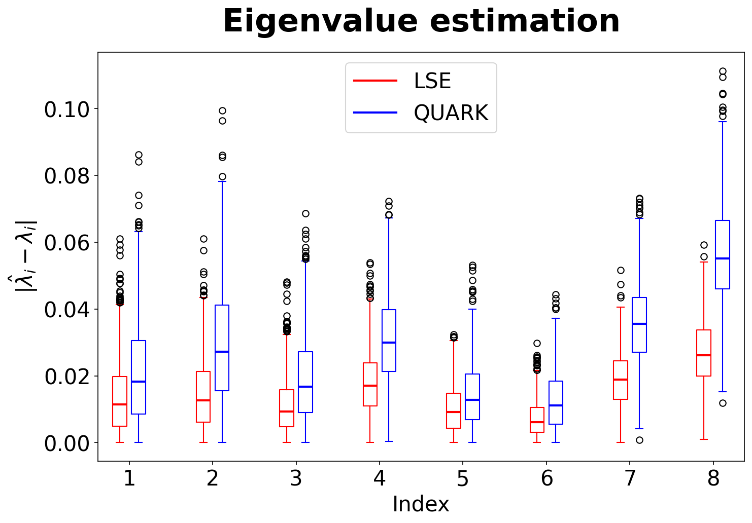
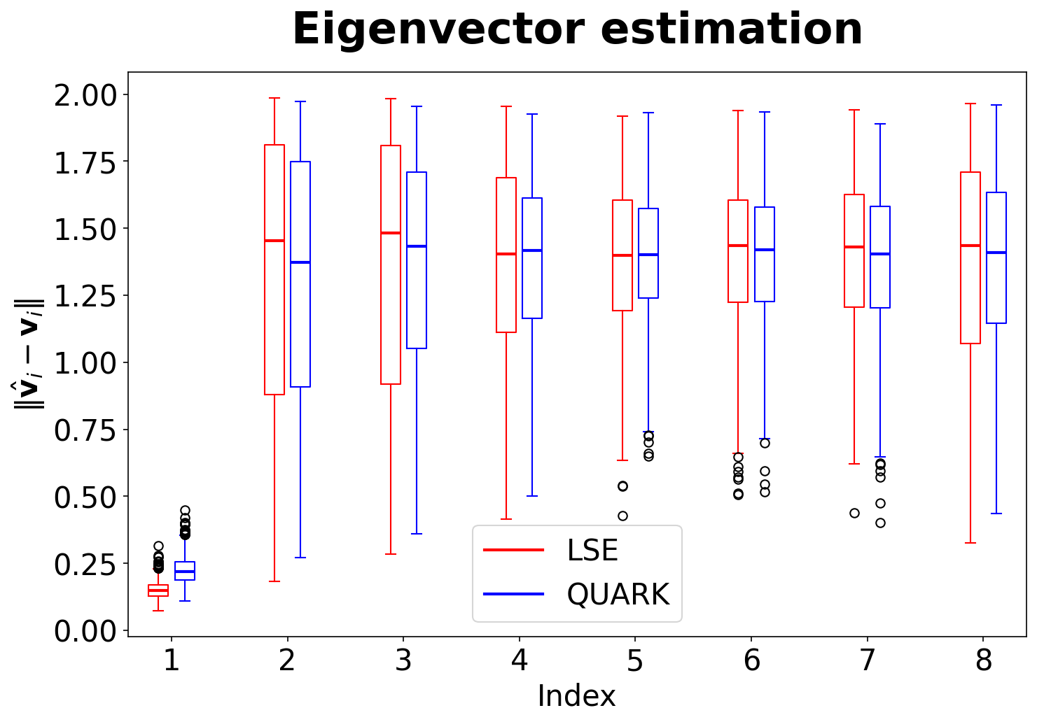
Refer to caption
Refer to caption
Figure 3: Spectral behavior of the LSE and QUARK estimator with kernel KK, based on 10001000 Monte Carlo repetitions. The boxplots are ordered by decreasing eigenvalue magnitude. Left: Absolute eigenvalue errors |λ^iLSE−λi||\hat{\lambda}^{\text{LSE}}_{i}-\lambda_{i}| (red) and |λ^iK−λi||\hat{\lambda}^{K}_{i}-\lambda_{i}| (blue). Right: Absolute eigenvector errors ‖𝐯^iLSE−𝐯i‖\|\hat{\mathbf{v}}^{\text{LSE}}_{i}-\mathbf{v}_{i}\| (red) and ‖𝐯^iK−𝐯i‖\|\hat{\mathbf{v}}_{i}^{K}-\mathbf{v}_{i}\| (blue).

Asymptotic Performances. We study the asymptotic behavior of the estimators as the number of samples per observable rr increases, varying r∈{2j:j=2,…,11}r\in\{2^{j}:j=2,\dots,11\}. We evaluate the reconstructions for the LSE (black), along with various QUARK estimators: KK (blue), K100K_{100} (orange), K0.01K_{0.01} (purple), and the polynomial kernel Kpoly​(x,y)=(1+⟨x,y⟩)2K_{\text{poly}}(x,y)=(1+\langle x,y\rangle)^{2} (green). These empirical results are compared to the benchmark theoretical MSE under an exact unitary design (with damping factor α𝒬=1/9\alpha_{\mathcal{Q}}=1/9) established in Theorem 4.14, denoted by the red dashed line. As shown in Fig. 4, the empirical behavior of the LSE closely tracks this theoretical scaling. While all QUARK estimators exhibit larger errors than the LSE, this gap diminishes as the bandwidth parameter cc increases. This reflects the fact that the Gaussian kernel approaches the 0–11 kernel (and thus the LSE behavior) as c→∞c\to\infty. Nonetheless, Fig. 4 validates the asymptotic decay rate predicted by the theory.

Refer to caption
Figure 4: Asymptotic performances in terms of MSE of the LSE and various QUARK estimators.

5.2 Entangled MUB versus Local Pauli

We compare the MUB design to Pauli design for a kk-qubit system (𝒬=ℂ2k\mathcal{Q}=\mathbb{C}^{2^{k}}). Standard approaches in the literature [15, 33, 35] often employs the full set of 4k4^{k} tensorized Pauli observables:

𝝈(i1,…,ik)=⨂j=1k𝝈ij,ij∈{0,x,y,z},𝝈0=𝐈2.\displaystyle\boldsymbol{\sigma}_{(i_{1},\dots,i_{k})}=\bigotimes_{j=1}^{k}\boldsymbol{\sigma}_{i_{j}},\quad i_{j}\in\{0,x,y,z\},\quad\boldsymbol{\sigma}_{0}=\mathbf{I}_{2}. (18)

We generate a true density matrix of low rank 33, and perform 2020 Monte Carlo simulations per setup. The left panel of Fig. 5 fixes k=6k=6 and compares the accuracy of our LSE estimator under a MUB design to the thresholding estimators under a Pauli design from [15], across varying sample sizes rr. The right panel illustrates the scaling behavior when the number of qubits increases (k=2,⋯,11k=2,\cdots,11). For a fair comparison, we fix the total sample size n⋅rn\cdot r across setups. As shown, our LSE under a MUB design tightly adheres to the theoretical performance of an exact unitary design. It outperforms the Pauli-based estimators by orders of magnitude (note the log scale), while being computationally exponentially faster: O​(k⋅2k)O(k\cdot 2^{k}) via the fast WHT (Section B.2) versus O​(4k)O(4^{k}).

Refer to caption
Refer to caption
Figure 5: Comparison between the proposed LSE estimator with MUB design and the Universal soft and hard thresholding estimators of [15] with Pauli designs. Left: dependence on the number of samples per observable. Right: dependence on the dimension of the quantum Hilbert space.

This performance gap is due to the high multiplicity inherent to Pauli observables: the identity yields a single trivial eigenvalue, while the remaining 4k−14^{k}-1 observables have spectra {±1}\{\pm 1\} with multiplicity 2k−12^{k-1}. Crucially, for k≥2k\geq 2, the tensor product design in (18) performs only local measurements and does not constitute a unitary design. To illustrate this, consider the trace-centering decomposition for k=2k=2: the space ℂs​a,04×4\mathbb{C}_{sa,0}^{4\times 4} splits into two local sectors ([ℂs​a,02×2⊗span{𝐈2}][\mathbb{C}_{sa,0}^{2\times 2}\otimes\operatorname*{span}\{\mathbf{I}_{2}\}] and [span{𝐈2}⊗ℂs​a,02×2][\operatorname*{span}\{\mathbf{I}_{2}\}\otimes\mathbb{C}_{sa,0}^{2\times 2}]) and one pure correlation sector ([ℂs​a,02×2⊗ℂs​a,02×2][\mathbb{C}_{sa,0}^{2\times 2}\otimes\mathbb{C}_{sa,0}^{2\times 2}]). The Gram superoperator 𝔇∗​𝔇/n\mathfrak{D}^{*}\mathfrak{D}/n acts diagonally on these subspaces with distinct eigenvalues. Since the local qubit design has αℂ2=1/3\alpha_{\mathbb{C}^{2}}=1/3, the eigenvalues for the local sectors are 1/31/3, whereas the eigenvalue for the correlation sector is the product (1/3)2(1/3)^{2}:

𝔇∗​𝔇n​𝝆=1⋅𝐈44⊕13​[𝚫A⊗𝐈22]⊕13​[𝐈22⊗𝚫B]⊕19​𝚫A​B,\displaystyle\frac{\mathfrak{D}^{*}\mathfrak{D}}{n}\boldsymbol{\rho}=1\cdot\frac{\mathbf{I}_{4}}{4}\oplus\frac{1}{3}\left[\boldsymbol{\Delta}_{A}\otimes\frac{\mathbf{I}_{2}}{2}\right]\oplus\frac{1}{3}\left[\frac{\mathbf{I}_{2}}{2}\otimes\boldsymbol{\Delta}_{B}\right]\oplus\frac{1}{9}\boldsymbol{\Delta}_{AB},

where 𝚫A=TrB​[𝝆]−𝐈2/2\boldsymbol{\Delta}_{A}=\mathrm{Tr}_{B}[\boldsymbol{\rho}]-\mathbf{I}_{2}/2 and 𝚫B=TrA​[𝝆]−𝐈2/2\boldsymbol{\Delta}_{B}=\mathrm{Tr}_{A}[\boldsymbol{\rho}]-\mathbf{I}_{2}/2 are the traceless marginals, and 𝚫A​B\boldsymbol{\Delta}_{AB} is the pure correlation tensor. This spectral gap widens exponentially with the number of qubits; the eigenvalue governing the kk-body correlation sector is (1/3)k(1/3)^{k}. Consequently, repeating the analysis of Theorem 4.14 reveals that the MSE scales as O​(9k/(n​r))O(9^{k}/(nr)) for a “worst-case” state dominated by global correlations. In contrast, the MUB design is an α𝒬\alpha_{\mathcal{Q}}-unitary design with α𝒬=(2k+1)−1\alpha_{\mathcal{Q}}=(2^{k}+1)^{-1} achieves O​(4k/(n​r))O(4^{k}/(nr)).

6 Discussion

This work establishes the kernel embedding theory to quantify how the geometry of the measurement process affects statistical efficiency. We demonstrate its utility for Quantum State Tomography, natively incorporating the least-squares approach under a metric-free topology.

Our theory of unitary design and minimax analysis, providing an analytical bound for the penalty incurred by eigenvalue degeneracies, clarifies the statistical price of quantum state recovery. Crucially, our analysis sheds a light on the fundamental tension between hardware implementation and statistical optimality: while local measurement schemes (e.g., tensorized Pauli) may yield optimal accuracy given strict sparsity assumptions tailored to that design, they incur a severe, exponential variance penalty. Achieving fundamental statistical efficiency strictly requires entangled observables, such as Mutually Unbiased Bases.

In contrast, by leveraging the spectral geometry of the measurement process rather than design-dependent sparsity, the proposed QUARK estimator provides a minimax-optimal framework for density estimation even in the highly entangled regimes where genuine quantum supremacy is realized.

{acks}

[Acknowledgments] Ho Yun is supported by a Swiss National Science Foundation granted to Victor Panaretos.

References

  • [1] J. Acharya, A. Dharmavarapu, Y. Liu, and N. Yu (2025) Pauli measurements are near-optimal for single-qubit tomography. arXiv preprint arXiv:2507.22001. Cited by: §1.
  • [2] F. T. Arecchi, E. Courtens, R. Gilmore, and H. Thomas (1972-12) Atomic coherent states in quantum optics. Phys. Rev. A 6, pp. 2211–2237. External Links: Document, Link Cited by: §1, §4.3.
  • [3] N. Aronszajn (1950) Theory of reproducing kernels. Trans. Am. Math. Soc. 68, pp. 337–404 (English). External Links: ISSN 0002-9947, Document Cited by: §3.1.
  • [4] L. M. Artiles, R. D. Gill, and M. I. Guță (2005) An invitation to quantum tomography. J. R. Stat. Soc., Ser. B, Stat. Methodol. 67 (1), pp. 109–134 (English). External Links: ISSN 1369-7412, Document Cited by: §1.
  • [5] F. Bach (2023) Information theory with kernel methods. IEEE Trans. Inf. Theory 69 (2), pp. 752–775 (English). External Links: ISSN 0018-9448, Document Cited by: §1, §1, §2.3, §2.3.
  • [6] P. Billingsley (2013) Convergence of probability measures. John Wiley & Sons. Cited by: Appendix D.
  • [7] R. Blume-Kohout (2010) Optimal, reliable estimation of quantum states. New Journal of Physics 12 (4), pp. 043034. Cited by: §2.3.
  • [8] S. Boucheron, G. Lugosi, and O. Bousquet (2004) Concentration inequalities. In Advanced Lectures on Machine Learning: ML Summer Schools 2003, Canberra, Australia, February 2 - 14, 2003, Tübingen, Germany, August 4 - 16, 2003, Revised Lectures, O. Bousquet, U. von Luxburg, and G. Rätsch (Eds.), pp. 208–240. External Links: ISBN 978-3-540-28650-9, Document, Link Cited by: Appendix D, Appendix D.
  • [9] S. P. Boyd and L. Vandenberghe (2004) Convex optimization. Cambridge university press. Cited by: §B.1.
  • [10] H. Breuer and F. Petruccione (2002) The theory of open quantum systems. Oxford: Oxford University Press (English). External Links: ISBN 0-19-852063-8 Cited by: §3.3.
  • [11] P. Busch, P. Lahti, J. Pellonpää, and K. Ylinen (2016) Quantum measurement. Theor. Math. Phys. (Cham), Cham: Springer (English). External Links: ISSN 1864-5879, ISBN 978-3-319-43387-5; 978-3-319-43389-9, Document Cited by: §3.3.
  • [12] P. Busch (1991-09-01) Informationally complete sets of physical quantities. International Journal of Theoretical Physics 30 (9), pp. 1217–1227. External Links: ISSN 1572-9575, Document, Link Cited by: Definition 4.1.
  • [13] C. Butucea, M. Guță, and L. Artiles (2007) Minimax and adaptive estimation of the Wigner function in quantum homodyne tomography with noisy data. Ann. Stat. 35 (2), pp. 465–494 (English). External Links: ISSN 0090-5364, Document Cited by: §1.
  • [14] C. Butucea, J. Johannes, and H. Stein (2025) Sample-optimal learning of quantum states using gentle measurements. arXiv preprint arXiv:2505.24587. Cited by: §4.2.
  • [15] T. Cai, D. Kim, Y. Wang, M. Yuan, and H. H. Zhou (2016) Optimal large-scale quantum state tomography with Pauli measurements. Ann. Stat. 44 (2), pp. 682–712 (English). External Links: ISSN 0090-5364, Document Cited by: §1, §2.3, Remark 4.7, Figure 5, §5.2, §5.2.
  • [16] C. Carmeli, E. de Vito, A. Toigo, and V. Umanità (2010) Vector valued reproducing kernel Hilbert spaces and universality. Anal. Appl., Singap. 8 (1), pp. 19–61 (English). External Links: ISSN 0219-5305, Document Cited by: §2.3.
  • [17] M. Christandl and R. Renner (2012-09) Reliable quantum state tomography. Phys. Rev. Lett. 109, pp. 120403. External Links: Document, Link Cited by: §1, §1.
  • [18] C. Cohen-Tannoudji, B. Diu, and F. Laloë (2020) Quantenmechanik. Band 3: Fermionen, Bosonen, Photonen, Korrelationen und Verschränkung. De Gruyter Stud., Berlin: De Gruyter (German). External Links: ISBN 978-3-11-062064-1; 978-3-11-064913-0, Document Cited by: §1, §2.2.
  • [19] B. Collins and P. Śniady (2006) Integration with respect to the Haar measure on unitary, orthogonal and symplectic group. Commun. Math. Phys. 264 (3), pp. 773–795 (English). External Links: ISSN 0010-3616, Document Cited by: Appendix D, item 2.
  • [20] J. B. Conway (1990) A course in functional analysis.. 2nd ed. edition, Grad. Texts Math., Vol. 96, New York etc.: Springer-Verlag (English). External Links: ISSN 0072-5285, ISBN 0-387-97245-5 Cited by: item 2, §2.1.
  • [21] J. B. Conway (2025) A course in operator theory. Vol. 21, American Mathematical Society. Cited by: footnote 1.
  • [22] M. Cramer, M. B. Plenio, S. T. Flammia, R. Somma, D. Gross, S. D. Bartlett, O. Landon-Cardinal, D. Poulin, and Y. Liu (2010-12-21) Efficient quantum state tomography. Nature Communications 1 (1), pp. 149. External Links: ISSN 2041-1723, Document, Link Cited by: §1, §1.
  • [23] G. M. D’Ariano, M. D. Laurentis, M. G. A. Paris, A. Porzio, and S. Solimeno (2002-03) Quantum tomography as a tool for the characterization of optical devices. Journal of Optics B: Quantum and Semiclassical Optics 4 (3), pp. S127. External Links: Document, Link Cited by: §1, §1.
  • [24] C. Davis and W. M. Kahan (1970) The rotation of eigenvectors by a perturbation. III. SIAM J. Numer. Anal. 7 (1), pp. 1–46 (English). External Links: ISSN 0036-1429, Document, Link Cited by: §5.1.
  • [25] J. Faraut (2008) Analysis on Lie groups. An introduction. Transl. from the French. Camb. Stud. Adv. Math., Vol. 110, Cambridge: Cambridge University Press (English). External Links: ISBN 978-0-521-71930-8 Cited by: item 1, §4.1.
  • [26] B. J. Fino and V. R. Algazi (1976) Unified matrix treatment of the fast Walsh-Hadamard transform. IEEE Trans. Comput. 25, pp. 1142–1146 (English). External Links: ISSN 0018-9340, Document Cited by: §1.
  • [27] S. T. Flammia, D. Gross, Y. Liu, and J. Eisert (2012) Quantum tomography via compressed sensing: error bounds, sample complexity and efficient estimators. New J. Phys. 14 (9), pp. 28 (English). Note: Id/No 095022 External Links: ISSN 1367-2630, Document Cited by: §1.
  • [28] K. Fukumizu, F. R. Bach, and M. I. Jordan (2004) Dimensionality reduction for supervised learning with reproducing kernel Hilbert spaces. J. Mach. Learn. Res. 5, pp. 73–99 (English). External Links: ISSN 1532-4435, Link Cited by: §1, §2.3, §3.2.
  • [29] T. N. Georges, B. K. Berntson, C. Sünderhauf, and A. V. Ivanov (2025-02) Pauli decomposition via the fast walsh-hadamard transform. New Journal of Physics 27 (3), pp. 033004. External Links: Document, Link Cited by: §1.
  • [30] D. Gottesman, A. Kitaev, and J. Preskill (2001-06) Encoding a qubit in an oscillator. Phys. Rev. A 64, pp. 012310. External Links: Document, Link Cited by: §C.1, §1, §4.3.
  • [31] D. Gottesman (1999) The Heisenberg representation of quantum computers. In Group 22: Proceedings of the XXII international colloquium on group theoretical methods in physics held in Hobart, Australia, July 13–17, 1998, pp. 32–43 (English). External Links: ISBN 1-57146-054-3 Cited by: §1.
  • [32] A. Gretton, K. M. Borgwardt, M. J. Rasch, B. Schölkopf, and A. Smola (2012) A kernel two-sample test. J. Mach. Learn. Res. 13, pp. 723–773 (English). External Links: ISSN 1532-4435, Link Cited by: §1, §2.3.
  • [33] D. Gross, Y. Liu, S. T. Flammia, S. Becker, and J. Eisert (2010-10) Quantum state tomography via compressed sensing. Phys. Rev. Lett. 105, pp. 150401. External Links: Document, Link Cited by: §1, §2.3, §4.2, Remark 4.7, §5.2.
  • [34] D. Gross (2011) Recovering low-rank matrices from few coefficients in any basis. IEEE Trans. Inf. Theory 57 (3), pp. 1548–1566 (English). External Links: ISSN 0018-9448, Document Cited by: §1.
  • [35] M. Guță, J. Kahn, R. Kueng, and J. A. Tropp (2020) Fast state tomography with optimal error bounds. J. Phys. A, Math. Theor. 53 (20), pp. 28 (English). Note: Id/No 204001 External Links: ISSN 1751-8113, Document Cited by: §5.2.
  • [36] H. Häffner, W. Hänsel, C. F. Roos, J. Benhelm, D. Chek-al-kar, M. Chwalla, T. Körber, U. D. Rapol, M. Riebe, P. O. Schmidt, C. Becher, O. Gühne, W. Dür, and R. Blatt (2005-12) Scalable multiparticle entanglement of trapped ions. Nature 438, pp. 643–646. External Links: Document, Link Cited by: §4.2.
  • [37] B. C. Hall (2013) Quantum theory for mathematicians. Grad. Texts Math., Vol. 267, New York, NY: Springer (English). External Links: ISSN 0072-5285, ISBN 978-1-4614-7115-8; 978-1-4614-7116-5, Document Cited by: Appendix A, Appendix D, item 1, §1, §2.2, §2.2, §2.2.
  • [38] S. G. Hoggar (1982) T-designs in projective spaces. Eur. J. Comb. 3, pp. 233–254 (English). External Links: ISSN 0195-6698, Document Cited by: §4.1.
  • [39] A. S. Holevo (2011) Probabilistic and statistical aspects of quantum theory. With a foreword from the second Russian edition by K. A. Valiev.. 2nd ed. edition, Quad., Sc. Norm. Super. Pisa, Monogr., Vol. 1, Pisa: Edizioni della Normale (English). External Links: ISBN 978-88-7642-375-8 Cited by: §1, §2.2, §2.2, §3.2.
  • [40] R. A. Horn and C. R. Johnson (2013) Matrix analysis.. 2nd ed. edition, Cambridge: Cambridge University Press (English). External Links: ISBN 978-0-521-54823-6; 978-0-521-83940-2 Cited by: §B.1.
  • [41] T. Hsing and R. Eubank (2015) Theoretical foundations of functional data analysis, with an introduction to linear operators. Wiley Ser. Probab. Stat., Hoboken, NJ: John Wiley & Sons (English). External Links: ISSN 1940-6347, ISBN 978-0-470-01691-6; 1-118-76254-1, Document Cited by: Appendix A, §3.1.
  • [42] R. V. Kadison and J. R. Ringrose (1986) Fundamentals of the theory of operator algebras. Volume II: Advanced theory. Pure Appl. Math., Academic Press, Vol. 100, Academic Press, New York, NY (English). External Links: ISSN 0079-8169 Cited by: Appendix D.
  • [43] A. Klappenecker and M. Rotteler (2005) Mutually unbiased bases are complex projective 2-designs. In Proceedings. International Symposium on Information Theory, 2005. ISIT 2005., Vol. , pp. 1740–1744. External Links: Document Cited by: item 1, §2.3, Remark 4.7.
  • [44] J. M. Lukens, K. J. H. Law, A. Jasra, and P. Lougovski (2020-06) A practical and efficient approach for bayesian quantum state estimation. New Journal of Physics 22 (6), pp. 063038. External Links: Document, Link Cited by: §2.3.
  • [45] K. Muandet, K. Fukumizu, B. Sriperumbudur, and B. Schölkopf (2017) Kernel mean embedding of distributions: a review and beyond. Found. Trends Mach. Learn. 10 (1-2), pp. 1–144 (English). External Links: ISSN 1935-8237, Document Cited by: §2.3.
  • [46] M. A. Nielsen and I. L. Chuang (2010) Quantum computation and quantum information. 10th anniversary edition. Cambridge: Cambridge University Press (English). External Links: ISBN 978-1-107-00217-3; 978-0-511-98524-9, Document Cited by: §1, §2.2, §2.3, §3.2.1, §3.3.1.
  • [47] V. I. Paulsen and M. Raghupathi (2016) An introduction to the theory of reproducing kernel Hilbert spaces. Camb. Stud. Adv. Math., Vol. 152, Cambridge: Cambridge University Press (English). External Links: ISBN 978-1-107-10409-9; 978-1-316-21923-2, Document Cited by: §3.1, Example 3.4, §4.3.
  • [48] D. T. Pegg and S. M. Barnett (1989-02) Phase properties of the quantized single-mode electromagnetic field. Phys. Rev. A 39, pp. 1665–1675. External Links: Document, Link Cited by: §1, §4.3.
  • [49] F. Pukelsheim (2006) Optimal design of experiments. Classics in Applied Mathematics, Vol. 50, SIAM. External Links: Document Cited by: item 1, §4.2.
  • [50] J. M. Renes, R. Blume-Kohout, A. J. Scott, and C. M. Caves (2004) Symmetric informationally complete quantum measurements.. J. Math. Phys. 45 (6), pp. 2171–2180 (English). External Links: ISSN 0022-2488, Document Cited by: footnote 3.
  • [51] J. J. Sakurai and J. Napolitano (2017) Modern quantum mechanics. 2nd edition edition, Cambridge: Cambridge University Press (English). External Links: ISBN 978-1-108-42241-3; 978-1-108-49999-6, Document Cited by: §3.2.1.
  • [52] A. J. Scott (2006) Tight informationally complete quantum measurements. J. Phys. A, Math. Gen. 39 (43), pp. 13507–13530 (English). External Links: ISSN 0305-4470, Document, Link Cited by: §4.1, §4.
  • [53] A. Smola, A. Gretton, L. Song, and B. Schölkopf (2007) A Hilbert space embedding for distributions. In Algorithmic learning theory. 18th international conference, ALT 2007, Sendai, Japan, October 1–4, 2007. Proceedings, pp. 13–31 (English). External Links: ISBN 978-3-540-75224-0, Document Cited by: §2.3, §3.1.
  • [54] J. A. Smolin, J. M. Gambetta, and G. Smith (2012-02) Efficient method for computing the maximum-likelihood quantum state from measurements with additive gaussian noise. Phys. Rev. Lett. 108, pp. 070502. External Links: Document, Link Cited by: §1, §4.2, §4.2.
  • [55] B. K. Sriperumbudur, A. Gretton, K. Fukumizu, G. R. G. Lanckriet, and B. Schölkopf (2008) Injective hilbert space embeddings of probability measures. Annual Conference Computational Learning Theory. Cited by: §1, §2.3.
  • [56] B. K. Sriperumbudur, A. Gretton, K. Fukumizu, B. Schölkopf, and G. R. G. Lanckriet (2010) Hilbert space embeddings and metrics on probability measures. J. Mach. Learn. Res. 11, pp. 1517–1561 (English). External Links: ISSN 1532-4435, Link Cited by: §1, §1, §2.3, §3.2.
  • [57] M. Talagrand (2022) What is a quantum field theory? A first introduction for mathematicians. Cambridge: Cambridge University Press (English). External Links: ISBN 978-1-316-51027-8; 978-1-108-22514-4, Document Cited by: §1, §2.2, Remark 3.14.
  • [58] A. B. Tsybakov (2009) Introduction to nonparametric estimation. Springer Ser. Stat., New York, NY: Springer (English). External Links: ISSN 0172-7397, ISBN 978-0-387-79051-0 Cited by: Appendix D.
  • [59] F. Verdeil and Y. Deville (2023-01) Pure-state tomography with parallel unentangled measurements. Phys. Rev. A 107, pp. 012408. External Links: Document, Link Cited by: §1.
  • [60] Y. Wang (2013) Asymptotic equivalence of quantum state tomography and noisy matrix completion. Ann. Stat. 41 (5), pp. 2462–2504 (English). External Links: ISSN 0090-5364, Document Cited by: §1.
  • [61] D. Xia (2017) Estimation of low rank density matrices by Pauli measurements. Electron. J. Stat. 11 (1), pp. 50–77 (English). External Links: ISSN 1935-7524, Document Cited by: §1.
  • [62] Y. Yang and A. Barron (1999) Information-theoretic determination of minimax rates of convergence. Ann. Stat. 27 (5), pp. 1564–1599 (English). External Links: ISSN 0090-5364, Document Cited by: Appendix D.
  • [63] K. Yosida (1980) Functional analysis. 6th ed. Grundlehren Math. Wiss., Vol. 123, Springer, Cham (English). External Links: ISSN 0072-7830 Cited by: Appendix A.
  • [64] Y. Yu, T. Wang, and R. J. Samworth (2015) A useful variant of the Davis-Kahan theorem for statisticians. Biometrika 102 (2), pp. 315–323 (English). External Links: ISSN 0006-3444, Document, Link Cited by: §5.1.
  • [65] G. Zauner (1999) Grundzüge einer nichtkommutativen designtheorie. Ph. D. dissertation, PhD thesis. Cited by: footnote 2.

Appendix A Tensorized Bochner integral

The usual Bochner integral for a general Hilbert (or Banach) space with respect to a scalar probability measure is typically constructed via a limiting argument over step functions [63, 41]. Here, we develop a tensorized Bochner integration where the measure is a Positive Operator-Valued Measure (POVM) and the Banach space of interest is the space of bounded operators on a Hilbert space, a formulation that natively supports our operator-theoretic framework.

Let ℋ1\mathcal{H}_{1} and ℋ2\mathcal{H}_{2} be Hilbert spaces. We define the inner product on elementary tensors by

⟨f1⊗f2,g1⊗g2⟩ℋ1⊗ℋ2:=⟨f1,g1⟩ℋ1​⟨f2,g2⟩ℋ2,f1,g1∈ℋ1,f2,g2∈ℋ2.{\left\langle{f_{1}\otimes f_{2}},{g_{1}\otimes g_{2}}\right\rangle}_{\mathcal{H}_{1}\otimes\mathcal{H}_{2}}:={\left\langle{f_{1}},{g_{1}}\right\rangle}_{\mathcal{H}_{1}}{\left\langle{f_{2}},{g_{2}}\right\rangle}_{\mathcal{H}_{2}},\quad f_{1},\,g_{1}\in\mathcal{H}_{1},\ f_{2},\,g_{2}\in\mathcal{H}_{2}.

For 𝐓1∈ℬ∞​(ℋ1)\mathbf{T}_{1}\in\mathcal{B}_{\infty}(\mathcal{H}_{1}) and 𝐓2∈ℬ∞​(ℋ2)\mathbf{T}_{2}\in\mathcal{B}_{\infty}(\mathcal{H}_{2}), there exists a unique bounded operator, denoted by 𝐓1⊗𝐓2∈ℬ∞​(ℋ1⊗ℋ2)\mathbf{T}_{1}\otimes\mathbf{T}_{2}\in\mathcal{B}_{\infty}(\mathcal{H}_{1}\otimes\mathcal{H}_{2}), such that

(𝐓1⊗𝐓2)​(f1⊗f2)=(𝐓1​f1)⊗(𝐓2​f2),(\mathbf{T}_{1}\otimes\mathbf{T}_{2})(f_{1}\otimes f_{2})=(\mathbf{T}_{1}f_{1})\otimes(\mathbf{T}_{2}f_{2}),

and it holds that ‖|𝐓1⊗𝐓2|‖∞=‖|𝐓1|‖∞​‖|𝐓2|‖∞{\left|\kern-1.07639pt\left|\kern-1.07639pt\left|\mathbf{T}_{1}\otimes\mathbf{T}_{2}\right|\kern-1.07639pt\right|\kern-1.07639pt\right|}_{\infty}={\left|\kern-1.07639pt\left|\kern-1.07639pt\left|\mathbf{T}_{1}\right|\kern-1.07639pt\right|\kern-1.07639pt\right|}_{\infty}{\left|\kern-1.07639pt\left|\kern-1.07639pt\left|\mathbf{T}_{2}\right|\kern-1.07639pt\right|\kern-1.07639pt\right|}_{\infty} [37, Proposition A.67]. Therefore, the quadratic form with respect to the elementary tensor entirely characterizes the tensorized operators. That is, for an operator 𝐓:(ℋ1⊗ℋ2)→(ℋ1⊗ℋ2)\mathbf{T}:(\mathcal{H}_{1}\otimes\mathcal{H}_{2})\to(\mathcal{H}_{1}\otimes\mathcal{H}_{2}), it holds that 𝐓=𝐓1⊗𝐓2\mathbf{T}=\mathbf{T}_{1}\otimes\mathbf{T}_{2} if and only if

⟨(𝐓1⊗𝐓2)​(f1⊗f2),g1⊗g2⟩ℋ1⊗ℋ2=⟨𝐓1​f1,g1⟩ℋ1​⟨𝐓2​f2,g2⟩ℋ2,\displaystyle{\left\langle{(\mathbf{T}_{1}\otimes\mathbf{T}_{2})(f_{1}\otimes f_{2})},{g_{1}\otimes g_{2}}\right\rangle}_{\mathcal{H}_{1}\otimes\mathcal{H}_{2}}={\left\langle{\mathbf{T}_{1}f_{1}},{g_{1}}\right\rangle}_{\mathcal{H}_{1}}{\left\langle{\mathbf{T}_{2}f_{2}},{g_{2}}\right\rangle}_{\mathcal{H}_{2}},

for any f1,g1∈ℋ1f_{1},g_{1}\in\mathcal{H}_{1} and f2,g2∈ℋ2f_{2},g_{2}\in\mathcal{H}_{2}. Hence, the formal definition below is well-posed:

Definition A.1.

Let 𝒬,ℋ\mathcal{Q},\mathcal{H} be Hilbert spaces. Let (X,ℬ​(X))(X,\mathscr{B}(X)) be an LCH space equipped with Borel σ\sigma-algebra, and 𝛎∈𝒫​(X,𝒬)\boldsymbol{\nu}\in\mathscr{P}(X,\mathcal{Q}) be a POVM. Consider the locally convex topological vector space ℬ∞​(ℋ)\mathcal{B}_{\infty}(\mathcal{H}) equipped with the Weak Operator Topology (WOT). A measurable function 𝐅:X→ℬ∞​(ℋ)\mathbf{F}:X\to\mathcal{B}_{\infty}(\mathcal{H}) is said to be tensorized Bochner integrable if there exists a bounded operator on ℋ⊗𝒬\mathcal{H}\otimes\mathcal{Q}, denoted by ∫X𝐅​(x)⊗d𝛎​(x)\int_{X}\mathbf{F}(x)\otimes\mathrm{d}\boldsymbol{\nu}(x), such that

⟨(∫X𝐅​(x)⊗d𝝂​(x))​(f⊗ϕ),g⊗ψ⟩ℋ⊗𝒬=∫X⟨𝐅​(x)​f,g⟩ℋ​d𝝂ϕ,ψ​(x),\displaystyle{\left\langle{\left(\int_{X}\mathbf{F}(x)\otimes\mathrm{d}\boldsymbol{\nu}(x)\right)(f\otimes\phi)},{g\otimes\psi}\right\rangle}_{\mathcal{H}\otimes\mathcal{Q}}=\int_{X}{\left\langle{\mathbf{F}(x)f},{g}\right\rangle}_{\mathcal{H}}\mathrm{d}\boldsymbol{\nu}_{\phi,\psi}(x), (19)

for any f,g∈ℋf,g\in\mathcal{H} and ϕ,ψ∈𝒬\phi,\psi\in\mathcal{Q}. We call ∫X𝐅​(x)⊗d𝛎​(x)\int_{X}\mathbf{F}(x)\otimes\mathrm{d}\boldsymbol{\nu}(x) the tensorized Bochner integral of 𝐅\mathbf{F} with respect to 𝛎\boldsymbol{\nu}.

In the case where ℋ=𝔽\mathcal{H}=\mathbb{F} or 𝒬=𝔽\mathcal{Q}=\mathbb{F}, this naturally reduces to the standard Bochner integral and functional calculus, respectively, where it is customary to write ∫X𝐅​(x)​d𝝂​(x)\int_{X}\mathbf{F}(x)\mathrm{d}\boldsymbol{\nu}(x) instead of ∫X𝐅​(x)⊗d𝝂​(x)\int_{X}\mathbf{F}(x)\otimes\mathrm{d}\boldsymbol{\nu}(x). Unlike the standard Bochner integral, we employ a topology strictly weaker than the norm topology. The WOT is sufficient to uniquely determine the integrated operator via its associated quadratic form. Furthermore, this choice allows us to leverage the Banach–Alaoglu theorem, which guarantees that the closed unit ball in (ℬ∞(ℋ),|||⋅|||∞)(\mathcal{B}_{\infty}(\mathcal{H}),{\left|\kern-1.07639pt\left|\kern-1.07639pt\left|\cdot\right|\kern-1.07639pt\right|\kern-1.07639pt\right|}_{\infty}) is compact with respect to the WOT. Consequently, if 𝐅\mathbf{F} is uniformly bounded, i.e., supx∈X‖|𝐅​(x)|‖∞<∞\sup_{x\in X}{\left|\kern-1.07639pt\left|\kern-1.07639pt\left|\mathbf{F}(x)\right|\kern-1.07639pt\right|\kern-1.07639pt\right|}_{\infty}<\infty, then it is automatically tensorized Bochner integrable since (19) remains bounded for all f,g∈ℋf,g\in\mathcal{H} and ϕ,ψ∈𝒬\phi,\psi\in\mathcal{Q}. In this bounded regime, we obtain the inequality: ‖|∫X𝐅⊗d𝝂|‖∞≤supx∈X‖|𝐅​(x)|‖∞{\left|\kern-1.07639pt\left|\kern-1.07639pt\left|\int_{X}\mathbf{F}\otimes\mathrm{d}\boldsymbol{\nu}\right|\kern-1.07639pt\right|\kern-1.07639pt\right|}_{\infty}\leq\sup_{x\in X}{\left|\kern-1.07639pt\left|\kern-1.07639pt\left|\mathbf{F}(x)\right|\kern-1.07639pt\right|\kern-1.07639pt\right|}_{\infty}. For a measurable simple function

𝐒​(x)=∑i=1n𝟙Bi​(x)​𝐒i,Bi∈ℬ​(X),𝐒i∈ℬ∞​(ℋ),n∈ℕ,\mathbf{S}(x)=\sum_{i=1}^{n}\mathds{1}_{B_{i}}(x)\mathbf{S}_{i},\quad B_{i}\in\mathscr{B}(X),\quad\mathbf{S}_{i}\in\mathcal{B}_{\infty}(\mathcal{H}),\quad n\in\mathbb{N},

its tensorized Bochner integral is trivially given by ∫X𝐒​(x)⊗d𝝂​(x)=∑i=1n𝐒i⊗𝝂​(Bi)∈ℬ∞​(ℋ⊗𝒬)\int_{X}\mathbf{S}(x)\otimes\mathrm{d}\boldsymbol{\nu}(x)=\sum_{i=1}^{n}\mathbf{S}_{i}\otimes\boldsymbol{\nu}(B_{i})\in\mathcal{B}_{\infty}(\mathcal{H}\otimes\mathcal{Q}), which is independent of the particular representation of the simple function 𝐒\mathbf{S}. Alternatively, one can construct the tensorized Bochner integral globally using a standard limiting argument:

Theorem A.2 (Lebesgue Dominated Convergence).

Let 𝒬\mathcal{Q} be a Hilbert space, and 𝛎∈𝒫​(X,𝒬)\boldsymbol{\nu}\in\mathscr{P}(X,\mathcal{Q}). An operator-valued measurable function 𝐅:X→(ℬ∞​(ℋ),WOT)\mathbf{F}:X\to(\mathcal{B}_{\infty}(\mathcal{H}),\mathrm{WOT}) is tensorized Bochner integrable if there exists a sequence of measurable simple functions {𝐒n:X→(ℬ∞​(ℋ),WOT)}n∈ℕ\{\mathbf{S}_{n}:X\to(\mathcal{B}_{\infty}(\mathcal{H}),\mathrm{WOT})\}_{n\in\mathbb{N}} such that:

  1. 1.

    There exists a scalar function h∈ℒ1​(X,𝝂)h\in\mathcal{L}_{1}(X,\boldsymbol{\nu}) (meaning hh is integrable with respect to the scalar positive measures 𝝂ϕ,ϕ\boldsymbol{\nu}_{\phi,\phi} for all ϕ∈𝒬\phi\in\mathcal{Q}) satisfying ‖|𝐒n​(x)|‖∞≤h​(x){\left|\kern-1.07639pt\left|\kern-1.07639pt\left|\mathbf{S}_{n}(x)\right|\kern-1.07639pt\right|\kern-1.07639pt\right|}_{\infty}\leq h(x) for any n∈ℕn\in\mathbb{N} and x∈Xx\in X.

  2. 2.

    For each x∈Xx\in X, 𝐒n​(x)→𝐅​(x)\mathbf{S}_{n}(x)\to\mathbf{F}(x) as n→∞n\to\infty with respect to the WOT in ℬ∞​(ℋ)\mathcal{B}_{\infty}(\mathcal{H}).

In this case, we have ‖|𝐅​(x)|‖∞≤h​(x){\left|\kern-1.07639pt\left|\kern-1.07639pt\left|\mathbf{F}(x)\right|\kern-1.07639pt\right|\kern-1.07639pt\right|}_{\infty}\leq h(x) for any x∈Xx\in X, and

∫X𝐅​(x)⊗d𝝂​(x)=limn→∞∫X𝐒n​(x)⊗d𝝂​(x),\displaystyle\int_{X}\mathbf{F}(x)\otimes\mathrm{d}\boldsymbol{\nu}(x)=\lim_{n\to\infty}\int_{X}\mathbf{S}_{n}(x)\otimes\mathrm{d}\boldsymbol{\nu}(x),

where the limit converges with respect to the WOT in ℬ∞​(ℋ⊗𝒬)\mathcal{B}_{\infty}(\mathcal{H}\otimes\mathcal{Q}).

Proof.

First, it is trivial that ‖|𝐅​(x)|‖∞≤h​(x){\left|\kern-1.07639pt\left|\kern-1.07639pt\left|\mathbf{F}(x)\right|\kern-1.07639pt\right|\kern-1.07639pt\right|}_{\infty}\leq h(x) for any x∈Xx\in X, since for any f,g∈ℋf,g\in\mathcal{H},

|⟨𝐅​(x)​f,g⟩ℋ|=limn→∞|⟨𝐒n​(x)​f,g⟩ℋ|≤h​(x)​‖f‖ℋ​‖g‖ℋ.|{\left\langle{\mathbf{F}(x)f},{g}\right\rangle}_{\mathcal{H}}|=\lim_{n\to\infty}|{\left\langle{\mathbf{S}_{n}(x)f},{g}\right\rangle}_{\mathcal{H}}|\leq h(x)\|f\|_{\mathcal{H}}\|g\|_{\mathcal{H}}.

Fix f,g∈ℋf,g\in\mathcal{H} and ϕ,ψ∈𝒬\phi,\psi\in\mathcal{Q}. Because |⟨𝐒n​(x)​f,g⟩ℋ|≤h​(x)​‖f‖ℋ​‖g‖ℋ|{\left\langle{\mathbf{S}_{n}(x)f},{g}\right\rangle}_{\mathcal{H}}|\leq h(x)\|f\|_{\mathcal{H}}\|g\|_{\mathcal{H}} and h∈ℒ1​(X,𝝂ϕ,ψ)h\in\mathcal{L}_{1}(X,\boldsymbol{\nu}_{\phi,\psi}), we can apply the standard Lebesgue dominated convergence theorem to obtain:

∫X⟨𝐅​(x)​f,g⟩ℋ​d𝝂ϕ,ψ​(x)\displaystyle\int_{X}{\left\langle{\mathbf{F}(x)f},{g}\right\rangle}_{\mathcal{H}}\mathrm{d}\boldsymbol{\nu}_{\phi,\psi}(x) =limn→∞∫X⟨𝐒n​(x)​f,g⟩ℋ​d𝝂ϕ,ψ​(x)\displaystyle=\lim_{n\to\infty}\int_{X}{\left\langle{\mathbf{S}_{n}(x)f},{g}\right\rangle}_{\mathcal{H}}\mathrm{d}\boldsymbol{\nu}_{\phi,\psi}(x)
=limn→∞⟨(∫X𝐒n​(x)⊗d𝝂​(x))​(f⊗ϕ),g⊗ψ⟩ℋ⊗𝒬.\displaystyle=\lim_{n\to\infty}{\left\langle{\left(\int_{X}\mathbf{S}_{n}(x)\otimes\mathrm{d}\boldsymbol{\nu}(x)\right)(f\otimes\phi)},{g\otimes\psi}\right\rangle}_{\mathcal{H}\otimes\mathcal{Q}}.

It suffices to show that the bounding limit is well-behaved for all f,g∈ℋf,g\in\mathcal{H} and ϕ,ψ∈𝒬\phi,\psi\in\mathcal{Q}. Define the bounded positive operator 𝐇:=∫Xh​(x)​d𝝂​(x)∈ℬ∞+​(𝒬)\mathbf{H}:=\int_{X}h(x)\mathrm{d}\boldsymbol{\nu}(x)\in\mathcal{B}_{\infty}^{+}(\mathcal{Q}), which is well-defined by the assumption h∈ℒ1​(X,𝝂)h\in\mathcal{L}_{1}(X,\boldsymbol{\nu}). By the Cauchy-Schwarz inequality for POVMs, the total variation of the complex measure satisfies d​|𝝂ϕ,ψ|​(x)≤d​𝝂ϕ,ϕ​(x)​d​𝝂ψ,ψ​(x)\mathrm{d}|\boldsymbol{\nu}_{\phi,\psi}|(x)\leq\sqrt{\mathrm{d}\boldsymbol{\nu}_{\phi,\phi}(x)\mathrm{d}\boldsymbol{\nu}_{\psi,\psi}(x)}.

Therefore, applying the Cauchy-Schwarz inequality for integrals, for any n∈ℕn\in\mathbb{N} we have:

|∫X⟨𝐒n​(x)​f,g⟩ℋ​d𝝂ϕ,ψ​(x)|≤‖f‖ℋ​‖g‖ℋ​∫Xh​(x)​d​|𝝂ϕ,ψ|​(x)\displaystyle\left|\int_{X}{\left\langle{\mathbf{S}_{n}(x)f},{g}\right\rangle}_{\mathcal{H}}\mathrm{d}\boldsymbol{\nu}_{\phi,\psi}(x)\right|\leq\|f\|_{\mathcal{H}}\|g\|_{\mathcal{H}}\int_{X}h(x)\mathrm{d}|\boldsymbol{\nu}_{\phi,\psi}|(x)
≤‖f‖ℋ​‖g‖ℋ​(∫Xh​(x)​d𝝂ϕ,ϕ​(x))1/2​(∫Xh​(x)​d𝝂ψ,ψ​(x))1/2\displaystyle\leq\|f\|_{\mathcal{H}}\|g\|_{\mathcal{H}}\left(\int_{X}h(x)\mathrm{d}\boldsymbol{\nu}_{\phi,\phi}(x)\right)^{1/2}\left(\int_{X}h(x)\mathrm{d}\boldsymbol{\nu}_{\psi,\psi}(x)\right)^{1/2}
=‖f‖ℋ​‖g‖ℋ​⟨𝐇​ϕ,ϕ⟩𝒬1/2​⟨𝐇​ψ,ψ⟩𝒬1/2≤‖f‖ℋ​‖g‖ℋ​‖|𝐇|‖∞​‖ϕ‖𝒬​‖ψ‖𝒬.\displaystyle=\|f\|_{\mathcal{H}}\|g\|_{\mathcal{H}}{\left\langle{\mathbf{H}\phi},{\phi}\right\rangle}_{\mathcal{Q}}^{1/2}{\left\langle{\mathbf{H}\psi},{\psi}\right\rangle}_{\mathcal{Q}}^{1/2}\leq\|f\|_{\mathcal{H}}\|g\|_{\mathcal{H}}{\left|\kern-1.07639pt\left|\kern-1.07639pt\left|\mathbf{H}\right|\kern-1.07639pt\right|\kern-1.07639pt\right|}_{\infty}\|\phi\|_{\mathcal{Q}}\|\psi\|_{\mathcal{Q}}.

This uniform bound over all nn strictly guarantees that the sesquilinear form defines a bounded operator on the tensor product space, completing the proof. ∎

Appendix B Algorithms for Quantum Tomography

B.1 Trace-Preserving Projection

Theorem B.1 (Sum-Preserving Threshold Algorithm (SPTA)).

Let 𝐚=(a1,⋯,aq)\mathbf{a}=(a_{1},\cdots,a_{q}) be a non-increasing real-valued sequence with a1+⋯+aq>0a_{1}+\cdots+a_{q}>0. Consider the following constrained optimization problem:

min​∑k=1q(ak−bk)2 w.r.t. b1≥⋯≥bq≥0, and ​b1+⋯+bq=a1+⋯+aq.\min\sum_{k=1}^{q}(a_{k}-b_{k})^{2}\quad\text{ w.r.t. }\quad b_{1}\geq\cdots\geq b_{q}\geq 0,\text{ and }b_{1}+\cdots+b_{q}=a_{1}+\cdots+a_{q}.

Define the truncation index and the truncated negative tail average by

t:=t​(𝐚)=max⁡{1≤k≤q:k​ak+ak+1+⋯+aq≥0},v:=v​(𝐚)=−at+1+⋯+aqt.\displaystyle t:=t(\mathbf{a})=\max\{1\leq k\leq q:ka_{k}+a_{k+1}+\dots+a_{q}\geq 0\},\,v:=v(\mathbf{a})=-\frac{a_{t+1}+\cdots+a_{q}}{t}.

Then, we have 0≤v≤at0\leq v\leq a_{t}, and the unique solution of the primal problem is achieved at SPTA​(𝐚):=𝐛∗=(b1∗,⋯,bq∗)\mathrm{SPTA}(\mathbf{a}):=\mathbf{b}^{*}=(b^{*}_{1},\cdots,b^{*}_{q}) with

bk∗={ak−v,k=1,2,⋯,t,0,k=t+1,t+2,⋯,q.b^{*}_{k}=\begin{cases}a_{k}-v&,\quad k=1,2,\cdots,t,\\ 0&,\quad k=t+1,t+2,\cdots,q.\end{cases}
Proof.

We may assume that a1+⋯+aq=1a_{1}+\cdots+a_{q}=1, as we can normalize the problem. We may further assume that aq<0a_{q}<0, otherwise the result is trivial as t=qt=q, v=0v=0 and 𝐛∗=𝐚\mathbf{b}^{*}=\mathbf{a}. Consider the sequence

sk:=k​ak+ak+1+⋯+aq,k=1,2,⋯,q.s_{k}:=ka_{k}+a_{k+1}+\dots+a_{q},\quad k=1,2,\cdots,q.

Then {sk:k=1,2,⋯,q}\{s_{k}:k=1,2,\cdots,q\} is a monotonically non-increasing sequence with s1=1s_{1}=1, since sk−sk+1=k​(ak−ak+1)≥0s_{k}-s_{k+1}=k(a_{k}-a_{k+1})\geq 0. This shows that t:=t​(𝐚)=max⁡{1≤k≤q:sk≥0}t:=t(\mathbf{a})=\max\{1\leq k\leq q:s_{k}\geq 0\} is well-defined. Also, the definition of tt yields v=−(at+1+⋯+aq)/t≤atv=-(a_{t+1}+\cdots+a_{q})/t\leq a_{t}. Note that

(t+1)​at+1+at+2+⋯+aq<0⇔v=−at+1+⋯+aqt>at+1,(t+1)a_{t+1}+a_{t+2}+\dots+a_{q}<0\quad\iff\quad v=-\frac{a_{t+1}+\cdots+a_{q}}{t}>a_{t+1},

hence v≥0v\geq 0. Otherwise, we have at+1<0a_{t+1}<0, but the monotonicity of 𝐚\mathbf{a} yields v>0v>0, which is a contradiction.

We now show that the sequence 𝐛∗\mathbf{b}^{*} satisfies the KKT conditions for the dual problem [9]:

L​(𝐛,𝐮,v)=12​∑k=1q(ak−bk)2+∑k=1quk​(−bk+bk+1)+v​(𝟏⊤​𝐛−1),\displaystyle L(\mathbf{b},\mathbf{u},v)=\frac{1}{2}\sum_{k=1}^{q}(a_{k}-b_{k})^{2}+\sum_{k=1}^{q}u_{k}(-b_{k}+b_{k+1})+v(\mathbf{1}^{\top}\mathbf{b}-1),

where bq+1:=0b_{q+1}:=0. Let v∗:=vv^{*}:=v, u0:=0u_{0}:=0, and uk∗:=k​v−∑i=1k(ai−bi∗)u^{*}_{k}:=kv-\sum_{i=1}^{k}(a_{i}-b^{*}_{i}) for k=1,2,⋯,qk=1,2,\cdots,q.

  1. 1.

    (Stationarity) For each k=1,⋯,qk=1,\cdots,q,

    ∂L​(𝐛,𝐮∗,v∗)∂bk|bk=bk∗=−(ak−bk∗)−(uk∗−uk−1∗)+v∗=0.\frac{\partial L(\mathbf{b},\mathbf{u}^{*},v^{*})}{\partial b_{k}}\Big|_{b_{k}=b^{*}_{k}}=-(a_{k}-b^{*}_{k})-(u^{*}_{k}-u^{*}_{k-1})+v^{*}=0.
  2. 2.

    (Primal Feasibility) We have

    b1∗≥⋯≥bt∗=at−v≥0=bt+1∗=⋯=bq∗,∑k=1qbk∗=∑k=1tak−t​v=∑k=1qak=1.\displaystyle b^{*}_{1}\geq\cdots\geq b^{*}_{t}=a_{t}-v\geq 0=b^{*}_{t+1}=\cdots=b^{*}_{q},\,\sum_{k=1}^{q}b^{*}_{k}=\sum_{k=1}^{t}a_{k}-tv=\sum_{k=1}^{q}a_{k}=1.
  3. 3.

    (Dual Feasibility) For k=1,⋯,tk=1,\cdots,t, uk∗=0u^{*}_{k}=0. Also, we have uq∗=q​v≥0u^{*}_{q}=qv\geq 0 and

    ut+1∗=ut∗+(v−at+1+bt+1∗)=v−at+1=−(t+1)​at+1+at+2+⋯+aqt≥0,\displaystyle u^{*}_{t+1}=u_{t}^{*}+(v-a_{t+1}+b^{*}_{t+1})=v-a_{t+1}=-\frac{(t+1)a_{t+1}+a_{t+2}+\cdots+a_{q}}{t}\geq 0,

    by the construction of tt, which yields

    uk∗=k​v−∑i=1k(ai−bi∗)=(k−t)​v−∑i=t+1kai≥(k−t)​(v−at+1)=(k−t)​ut+1∗≥0,\displaystyle u^{*}_{k}=kv-\sum_{i=1}^{k}(a_{i}-b^{*}_{i})=(k-t)v-\sum_{i=t+1}^{k}a_{i}\geq(k-t)(v-a_{t+1})=(k-t)u^{*}_{t+1}\geq 0,

    for k=t+2,⋯,q−1k=t+2,\cdots,q-1.

  4. 4.

    (Complementary Slackness) For k=1,⋯,tk=1,\cdots,t, we have uk∗​(−bk∗+bk+1∗)=0u^{*}_{k}(-b^{*}_{k}+b^{*}_{k+1})=0 since uk∗=0u^{*}_{k}=0. For k=t+1,⋯,qk=t+1,\cdots,q, we also have uk∗​(−bk∗+bk+1∗)=0u^{*}_{k}(-b^{*}_{k}+b^{*}_{k+1})=0 since bk∗=bk+1∗=0b^{*}_{k}=b^{*}_{k+1}=0.

∎

Algorithm 1 Sum-Preserving Threshold Algorithm (SPTA)
1:𝐚=(a1,⋯,aq)∈ℝq\mathbf{a}=(a_{1},\cdots,a_{q})\in\mathbb{R}^{q} with a1≥⋯≥aqa_{1}\geq\cdots\geq a_{q} and a1+⋯+aq>0a_{1}+\cdots+a_{q}>0
2:𝐛=(b1,⋯,bq)∈ℝq\mathbf{b}=(b_{1},\cdots,b_{q})\in\mathbb{R}^{q} with b1≥⋯≥bq≥0b_{1}\geq\cdots\geq b_{q}\geq 0 and 𝟏⊤​𝐛=𝟏⊤​𝐚\mathbf{1}^{\top}\mathbf{b}=\mathbf{1}^{\top}\mathbf{a}
3:procedure SPTA(𝐚\mathbf{a})
4:  if aq≥0a_{q}\geq 0 then ⊳\triangleright If all elements are non-negative, 𝐚\mathbf{a} is the solution
5:   return 𝐚\mathbf{a}   
6:  Sum←0\text{Sum}\leftarrow 0 ⊳\triangleright Stores the running sum of the tail, ak+1+⋯+aqa_{k+1}+\dots+a_{q}
7:  k←qk\leftarrow q
8:⊳\triangleright Phase 1: Efficiently scan past the negative tail.
9:  while ak≤0a_{k}\leq 0 do
10:   Sum←Sum+ak\text{Sum}\leftarrow\text{Sum}+a_{k}
11:   k←k−1k\leftarrow k-1   
12:⊳\triangleright Phase 2: Find the true truncation index, starting from the first positive value.
13:  while k⋅ak+Sum<0k\cdot a_{k}+\text{Sum}<0 do
14:   Sum←Sum+ak\text{Sum}\leftarrow\text{Sum}+a_{k}
15:   k←k−1k\leftarrow k-1   
16:  𝐛←(0,0,⋯,0)\mathbf{b}\leftarrow(0,0,\cdots,0) ⊳\triangleright Initialize as a zero vector.
17:  Shift←Sum/k\text{Shift}\leftarrow\text{Sum}/k ⊳\triangleright Shift is −v-v, where vv is the corrective offset
18:  for i←1i\leftarrow 1 to kk do
19:   bi←ai+Shiftb_{i}\leftarrow a_{i}+\text{Shift} ⊳\triangleright Apply the shift to the head of the vector   
20:  return 𝐛\mathbf{b} ⊳\triangleright The tail of 𝐛\mathbf{b} remains zero

In the case where 𝐚\mathbf{a} contains only a small number of negative values, it is computationally more efficient to compute sks_{k} backwards, starting from the first non-negative value. The SPTA algorithm can readily be used to project a self-adjoint matrix onto the convex set of n.n.d. matrices with respect to the Frobenius norm:

Table 1: Execution trace of SPTA (Algorithm 1) with q=7q=7 and 𝐚=(1.1,0.3,0.1,0.1,−0.1,−0.2,−0.3)\mathbf{a}=(1.1,0.3,0.1,0.1,-0.1,-0.2,-0.3).
Phase kk aka_{k} Sum Condition Check Result
Phase 1: Scan non-positive tail (ak≤0a_{k}\leq 0)
Start 7 -0.3 0 a7≤0a_{7}\leq 0 True
Iter 1 6 -0.2 -0.3 a6≤0a_{6}\leq 0 True
Iter 2 5 -0.1 -0.5 a5≤0a_{5}\leq 0 True
Iter 3 4 0.1 -0.6 a4≤0a_{4}\leq 0 False
Phase 2: Find truncation index (k⋅ak+Sum<0k\cdot a_{k}+\text{Sum}<0)
Start 4 0.1 -0.6 4​(0.1)+(−0.6)=−0.24(0.1)+(-0.6)=-0.2 True
Iter 1 3 0.1 -0.5 3​(0.1)+(−0.5)=−0.23(0.1)+(-0.5)=-0.2 True
Iter 2 2 0.3 -0.4 2​(0.3)+(−0.4)=0.22(0.3)+(-0.4)=0.2 False
Final Calculation
Loop terminates with k=2k=2 and Sum=−0.4\texttt{Sum}=-0.4.
Calculate Shift: Shift=Sum/k=−0.2\texttt{Shift}=\texttt{Sum}/k=-0.2.
Construct 𝐛\mathbf{b}: b1=1.1−0.2=0.9b_{1}=1.1-0.2=0.9, b2=0.3−0.2=0.1b_{2}=0.3-0.2=0.1. The rest are 0.
Result: 𝐛=(0.9,0.1,0,0,0,0,0)\mathbf{b}=(0.9,0.1,0,0,0,0,0).
Theorem B.2 (Trace-preserving projection).

Let 𝐒=𝐔​Diag⁡[𝐚]​𝐔∗∈𝔽s​aq×q\mathbf{S}=\mathbf{U}\operatorname{Diag}[\mathbf{a}]\mathbf{U}^{*}\in\mathbb{F}_{sa}^{q\times q} be the spectral decomposition of a self-adjoint matrix, where 𝐔\mathbf{U} is unitary (orthogonal if 𝔽=ℝ\mathbb{F}=\mathbb{R}) matrix and 𝐚=(a1,…,aq)\mathbf{a}=(a_{1},\dots,a_{q}) is the vector of its real eigenvalues, sorted in non-increasing order. Then the optimization problem

arg⁡min𝐓∈𝔽s​aq×q⁡|‖𝐒−𝐓‖|22 w.r.t. 𝐓⪰𝟎andTr⁡[𝐓]=Tr⁡[𝐒],\operatorname*{\arg\min}_{\mathbf{T}\in\mathbb{F}_{sa}^{q\times q}}{\left|\kern-1.07639pt\left|\kern-1.07639pt\left|\mathbf{S}-\mathbf{T}\right|\kern-1.07639pt\right|\kern-1.07639pt\right|}_{2}^{2}\quad\text{ w.r.t. }\quad\mathbf{T}\succeq\mathbf{0}\quad\text{and}\quad\operatorname{Tr}\left[\mathbf{T}\right]=\operatorname{Tr}\left[\mathbf{S}\right],

has a unique solution given by 𝐔​Diag⁡[SPTA​(𝐚)]​𝐔∗\mathbf{U}\operatorname{Diag}[\mathrm{SPTA}(\mathbf{a})]\mathbf{U}^{*}.

Proof.

Using spectral decomposition, we solve the optimization problem in two steps:

min𝐃=Diag⁡[𝐛]⁡(min𝐕∈S​U​(q)∣‖𝐕𝐃𝐕∗−𝐒‖|22) w.r.t. 𝐃⪰𝟎​ and ​Tr⁡[𝐃]=Tr⁡[𝐒],\min_{\mathbf{D}=\operatorname{Diag}[\mathbf{b}]}\left(\min_{\mathbf{V}\in SU(q)}{\left|\kern-1.07639pt\left|\kern-1.07639pt\left|\mathbf{V}\mathbf{D}\mathbf{V}^{*}-\mathbf{S}\right|\kern-1.07639pt\right|\kern-1.07639pt\right|}_{2}^{2}\right)\quad\text{ w.r.t. }\quad\mathbf{D}\succeq\mathbf{0}\text{ and }\operatorname{Tr}\left[\mathbf{D}\right]=\operatorname{Tr}\left[\mathbf{S}\right],

where 𝐛\mathbf{b} is also sorted in non-increasing order. For a fixed diagonal matrix 𝐃⪰𝟎\mathbf{D}\succeq\mathbf{0} with Tr⁡[𝐃]=Tr⁡[𝐒]\operatorname{Tr}\left[\mathbf{D}\right]=\operatorname{Tr}\left[\mathbf{S}\right], the inner optimization problem becomes

min𝐕∈S​U​(q)⁡|‖𝐕𝐃𝐕∗−𝐒‖|22\displaystyle\min_{\mathbf{V}\in SU(q)}{\left|\kern-1.07639pt\left|\kern-1.07639pt\left|\mathbf{V}\mathbf{D}\mathbf{V}^{*}-\mathbf{S}\right|\kern-1.07639pt\right|\kern-1.07639pt\right|}_{2}^{2} =|||𝐃|||22+|||𝐒|||22−2max𝐕∈S​U​(q)⟨𝐕𝐃𝐕∗,𝐒⟩2\displaystyle={\left|\kern-1.07639pt\left|\kern-1.07639pt\left|\mathbf{D}\right|\kern-1.07639pt\right|\kern-1.07639pt\right|}_{2}^{2}+{\left|\kern-1.07639pt\left|\kern-1.07639pt\left|\mathbf{S}\right|\kern-1.07639pt\right|\kern-1.07639pt\right|}_{2}^{2}-2\max_{\mathbf{V}\in SU(q)}{\left\langle{\mathbf{V}\mathbf{D}\mathbf{V}^{*}},{\mathbf{S}}\right\rangle}_{2}

by the von-Neumann trace inequality [40], and equality holds if and only if 𝐔=𝐕\mathbf{U}=\mathbf{V}. Consequently, the outer optimization problem simplifies to Theorem B.1. ∎

B.2 Tomography with Mutually Unbiased Bases

Let G​F​(2k)GF(2^{k}) be the Galois Field of order q=2kq=2^{k} equipped with operations (∙,+)(\bullet,+). We view elements of G​F​(2k)GF(2^{k}) strictly as polynomials modulo an irreducible polynomial pk​(x)p_{k}(x) of degree kk. To identify field operations with vector operations, we assume the choice of a self-dual basis for G​F​(2k)GF(2^{k}). Under this basis, the field trace creates an isomorphism to the standard Euclidean dot product:

TrG​F​(𝐚∙𝐛)=𝐚⊤​𝐛=∑j=1kaj​bj(mod2),𝐚,𝐛,𝐜,𝐝∈{0,1}k\displaystyle\text{Tr}_{GF}(\mathbf{a}\bullet\mathbf{b})=\mathbf{a}^{\top}\mathbf{b}=\sum_{j=1}^{k}a_{j}b_{j}\pmod{2},\quad\mathbf{a},\mathbf{b},\mathbf{c},\mathbf{d}\in\{0,1\}^{k}

For instance, (011)∙(111)=(010)(011)\bullet(111)=(010), because (x+1)​(x2+x+1)≡x(modp3)(x+1)(x^{2}+x+1)\equiv x\pmod{p_{3}}, where the arithmetic is modulo the irreducible polynomial p3​(x)=x3+x+1p_{3}(x)=x^{3}+x+1. The phase space is the vector space G​F​(2k)×G​F​(2k)GF(2^{k})\times GF(2^{k}), and its elements are denoted by 𝐮=(𝐚|𝐛)\mathbf{u}=(\mathbf{a}|\mathbf{b}). Under the self-dual basis, we can define the symplectic inner product consistently for both the field and the vector space:

⟨(𝐚|𝐛),(𝐜|𝐝)⟩s​p=𝐚⊤​𝐝+𝐛⊤​𝐜(mod2).{\left\langle{(\mathbf{a}|\mathbf{b})},{(\mathbf{c}|\mathbf{d})}\right\rangle}_{sp}=\mathbf{a}^{\top}\mathbf{d}+\mathbf{b}^{\top}\mathbf{c}\pmod{2}. (20)

This phase space corresponds to the Pauli operators of the kk-qubit system 𝒬=ℂq\mathcal{Q}=\mathbb{C}^{q}, having size q2=22​kq^{2}=2^{2k}:

𝐈2=(1001),𝐗=(0110),𝐘p​h​y=(0−ıı0),𝐙=(100−1)∈ℂs​a,02×2.\mathbf{I}_{2}=\begin{pmatrix}1&0\\ 0&1\end{pmatrix},\quad\mathbf{X}=\begin{pmatrix}0&1\\ 1&0\end{pmatrix},\quad\mathbf{Y}^{phy}=\begin{pmatrix}0&-\imath\\ \imath&0\end{pmatrix},\quad\mathbf{Z}=\begin{pmatrix}1&0\\ 0&-1\end{pmatrix}\in\mathbb{C}_{sa,0}^{2\times 2}.

We define the mathematical Pauli Y matrix by 𝐘m​a​t​h=𝐗𝐙\mathbf{Y}^{math}=\mathbf{X}\mathbf{Z} so that 𝐘p​h​y=ı​𝐘m​a​t​h\mathbf{Y}^{phy}=\imath\mathbf{Y}^{math}. For the kk-qubit system 𝒬=ℂq\mathcal{Q}=\mathbb{C}^{q} with q=2kq=2^{k}, the mathematical tensorized Pauli operators can be identified with the symplectic vector space (ℤ22​k,⟨⋅,⋅⟩s​p)(\mathbb{Z}_{2}^{2k},{\left\langle{\cdot},{\cdot}\right\rangle}_{sp}):

𝐏𝐮m​a​t​h=⨂j=1k𝐗jaj​𝐙jbj,𝐮=(𝐚|𝐛).\displaystyle\mathbf{P}_{\mathbf{u}}^{math}=\bigotimes_{j=1}^{k}\mathbf{X}_{j}^{a_{j}}\mathbf{Z}_{j}^{b_{j}},\quad\mathbf{u}=(\mathbf{a}|\mathbf{b}).

For instance, as 𝐈2↔(0|0)\mathbf{I}_{2}\leftrightarrow(0|0), 𝐗↔(1|0)\mathbf{X}\leftrightarrow(1|0), 𝐘m​a​t​h↔(1|1)\mathbf{Y}^{math}\leftrightarrow(1|1), 𝐙↔(0|1)\mathbf{Z}\leftrightarrow(0|1), the vector 𝐮=(1010|0011)\mathbf{u}=(1010|0011) determines 𝐏𝐮m​a​t​h=𝐗𝐈2​𝐘m​a​t​h​𝐙\mathbf{P}_{\mathbf{u}}^{math}=\mathbf{X}\mathbf{I}_{2}\mathbf{Y}^{math}\mathbf{Z}. In this association, the commutative relationship between Pauli operators can be written as

𝐏𝐮​𝐏𝐯=ı⟨𝐮,𝐯⟩s​p​𝐏𝐮+𝐯=(−1)⟨𝐮,𝐯⟩s​p​𝐏𝐯​𝐏𝐮⇒⟨𝐮,𝐯⟩s​p={0,commute,1,anti-commute,\displaystyle\mathbf{P}_{\mathbf{u}}\mathbf{P}_{\mathbf{v}}=\imath^{{\left\langle{\mathbf{u}},{\mathbf{v}}\right\rangle}_{sp}}\mathbf{P}_{\mathbf{u}+\mathbf{v}}=(-1)^{{\left\langle{\mathbf{u}},{\mathbf{v}}\right\rangle}_{sp}}\mathbf{P}_{\mathbf{v}}\mathbf{P}_{\mathbf{u}}\,\Rightarrow\,{\left\langle{\mathbf{u}},{\mathbf{v}}\right\rangle}_{sp}=\begin{cases}0&,\quad\text{commute},\\ 1&,\quad\text{anti-commute},\end{cases} (21)

and here the choice of physical or mathematical convention does not matter for commutativity.

A clique is a maximal subgroup of mutually commutative Pauli operators. There are q+1q+1 cliques consisting of q−1q-1 traceless Pauli operators and the identity 𝐈q\mathbf{I}_{q}. Each clique is associated with a label 𝝀∈{0,1}k∪{∞}\boldsymbol{\lambda}\in\{0,1\}^{k}\cup\{\infty\}. The generators for these cliques are derived from the field structure. In the bitwise representation with 𝐞0=(100​⋯​0),𝐞1=(010​⋯​0),⋯,𝐞k−1=(000​⋯​01)\mathbf{e}_{0}=(100\cdots 0),\mathbf{e}_{1}=(010\cdots 0),\cdots,\mathbf{e}_{k-1}=(000\cdots 01), these are given by:

  • •

    (λ=∞\boldsymbol{\lambda}=\infty) The clique is given by 𝒞∞={(𝟎|𝐛):𝐛∈{0,1}k}\mathcal{C}_{\infty}=\{(\mathbf{0}|\mathbf{b}):\mathbf{b}\in\{0,1\}^{k}\}, generated by 𝒢∞={(𝟎|𝐞j):1≤j≤k}\mathcal{G}_{\infty}=\{(\mathbf{0}|\mathbf{e}_{j}):1\leq j\leq k\}. This is the computational basis, as the generator simply matches the Pauli Z operators for each qubit.

  • •

    (λ∈{0,1}k\boldsymbol{\lambda}\in\{0,1\}^{k}) The clique is given by 𝒞𝝀={(𝐚|λ∙𝐚):𝐚∈{0,1}k}\mathcal{C}_{\boldsymbol{\lambda}}=\{(\mathbf{a}|\lambda\bullet\mathbf{a}):\mathbf{a}\in\{0,1\}^{k}\}, generated by 𝒢𝝀={(𝐞j|𝝀∙𝐞j):0≤j≤k−1}\mathcal{G}_{\boldsymbol{\lambda}}=\{(\mathbf{e}_{j}|\boldsymbol{\lambda}\bullet\mathbf{e}_{j}):0\leq j\leq k-1\}.

Let us denote the physical generators by 𝐆𝝀,jp​h​y=𝐏(𝐞j|𝝀∙𝐞j)p​h​y\mathbf{G}_{\boldsymbol{\lambda},j}^{phy}=\mathbf{P}_{(\mathbf{e}_{j}|\boldsymbol{\lambda}\bullet\mathbf{e}_{j})}^{phy} (it is obvious for 𝐙j=𝐆∞,jp​h​y\mathbf{Z}_{j}=\mathbf{G}_{\infty,j}^{phy}). Because the operators in a clique commute, they share a common eigenbasis, which serves as an orthonormal basis of ℂq\mathbb{C}^{q}. Each clique determined by 𝝀∈{0,1}k∪{∞}\boldsymbol{\lambda}\in\{0,1\}^{k}\cup\{\infty\} and 𝐚∈{0,1}k\mathbf{a}\in\{0,1\}^{k} amounts to the physical eigenspace:

𝚷𝝀,𝐚p​h​y=∏j=1k𝐈2+(−1)aj​𝐆𝝀,jp​h​y2=12k​∑𝐛∈G​F​(2k)(−1)𝐚⊤​𝐛​ϕ𝝀​(𝐛)​𝐏(𝐛|𝝀∙𝐛)p​h​y\displaystyle\mathbf{\Pi}_{\boldsymbol{\lambda},\mathbf{a}}^{phy}=\prod_{j=1}^{k}\frac{\mathbf{I}_{2}+(-1)^{a_{j}}\mathbf{G}_{\boldsymbol{\lambda},j}^{phy}}{2}=\frac{1}{2^{k}}\sum_{\mathbf{b}\in GF(2^{k})}(-1)^{\mathbf{a}^{\top}\mathbf{b}}\phi_{\boldsymbol{\lambda}}(\mathbf{b})\mathbf{P}_{(\mathbf{b}|\boldsymbol{\lambda}\bullet\mathbf{b})}^{phy}

where ϕ𝝀​(𝐛)∈{±1}\phi_{\boldsymbol{\lambda}}(\mathbf{b})\in\{\pm 1\} is the phase correction arising from (21):

∏j:bj=1𝐆𝝀,jp​h​y=ϕ𝝀​(𝐛)​𝐏(𝐛|𝝀∙𝐛)p​h​y.\displaystyle\prod_{j:b_{j}=1}\mathbf{G}_{\boldsymbol{\lambda},j}^{phy}=\phi_{\boldsymbol{\lambda}}(\mathbf{b})\mathbf{P}_{(\mathbf{b}|\boldsymbol{\lambda}\bullet\mathbf{b})}^{phy}.

The q+1q+1 collection of orthonormal bases (with identifications via the eigenspace) {𝚷𝝀,𝐚p​h​y:𝐚∈{0,1}k}𝝀\{\mathbf{\Pi}_{\boldsymbol{\lambda},\mathbf{a}}^{phy}:\mathbf{a}\in\{0,1\}^{k}\}_{\boldsymbol{\lambda}} is called the MUB.

Any self-adjoint matrix on the kk-qubit system 𝒬=ℂq\mathcal{Q}=\mathbb{C}^{q} can be decomposed into the Pauli basis

𝝆=12k​∑𝐮∈{0,1}2​k𝐫𝐮​𝐏𝐮p​h​y∈ℂs​aq×q.\displaystyle\boldsymbol{\rho}=\frac{1}{2^{k}}\sum_{\mathbf{u}\in\{0,1\}^{2k}}\mathbf{r}_{\mathbf{u}}\mathbf{P}_{\mathbf{u}}^{phy}\in\mathbb{C}_{sa}^{q\times q}.

Hence, 𝐫∈ℝq2\mathbf{r}\in\mathbb{R}^{q^{2}} is called the generalized Bloch vector. If 𝝆∈𝕊​(ℂ+q×q)\boldsymbol{\rho}\in\mathbb{S}(\mathbb{C}_{+}^{q\times q}) is a density matrix, then 𝐫(𝟎|𝟎)=Tr⁡[𝝆]=1\mathbf{r}_{(\mathbf{0}|\mathbf{0})}=\operatorname{Tr}\left[\boldsymbol{\rho}\right]=1, and the coefficients give the expected probability of the Bernoulli distribution under the Pauli observable. In contrast, under the MUB tomography, the expected probabilities are given by the Walsh–Hadamard Transform (WHT) of the Bloch vector: for 𝝀∈{0,1}k∪{∞},𝐚∈{0,1}k\boldsymbol{\lambda}\in\{0,1\}^{k}\cup\{\infty\},\mathbf{a}\in\{0,1\}^{k},

d𝝀,𝐚​[𝝆]=Tr​(𝝆​𝚷𝝀,𝐚p​h​y)=12k​∑𝐛∈{0,1}k(−1)𝐚⊤​𝐛​ϕ𝝀​(𝐛)​𝐫(𝐛|𝝀∙𝐛),\displaystyle d_{\boldsymbol{\lambda},\mathbf{a}}[\boldsymbol{\rho}]=\text{Tr}(\boldsymbol{\rho}\mathbf{\Pi}_{\boldsymbol{\lambda},\mathbf{a}}^{phy})=\frac{1}{2^{k}}\sum_{\mathbf{b}\in\{0,1\}^{k}}(-1)^{\mathbf{a}^{\top}\mathbf{b}}\phi_{\boldsymbol{\lambda}}(\mathbf{b})\mathbf{r}_{(\mathbf{b}|\boldsymbol{\lambda}\bullet\mathbf{b})},

which is the Walsh–Hadamard Transform of the Bloch vector restricted to the clique defined by 𝝀\boldsymbol{\lambda}. If p𝝀,𝐚∼Binom​(r,d𝝀,𝐚​[𝝆])/rp_{\boldsymbol{\lambda},\mathbf{a}}\sim\text{Binom}(r,d_{\boldsymbol{\lambda},\mathbf{a}}[\boldsymbol{\rho}])/r is the estimate for d𝝀,𝐚​[𝝆]d_{\boldsymbol{\lambda},\mathbf{a}}[\boldsymbol{\rho}], then the LSE under the MUB tomography is given by

𝝆^LSE=∑𝝀∈{0,1}k∪{∞}∑𝐚∈{0,1}kp𝝀,𝐚​𝚷𝝀,𝐚−𝐈q.\displaystyle\hat{\boldsymbol{\rho}}^{\text{LSE}}=\sum_{\boldsymbol{\lambda}\in\{0,1\}^{k}\cup\{\infty\}}\sum_{\mathbf{a}\in\{0,1\}^{k}}p_{\boldsymbol{\lambda},\mathbf{a}}\mathbf{\Pi}_{\boldsymbol{\lambda},\mathbf{a}}-\mathbf{I}_{q}.

To simply compute its generalized Bloch vector, we can use the inverse WHT: for 𝝀∈{0,1}k∪{∞},𝐛∈{0,1}k\{𝟎}\boldsymbol{\lambda}\in\{0,1\}^{k}\cup\{\infty\},\mathbf{b}\in\{0,1\}^{k}\backslash\{\mathbf{0}\},

𝐫^(𝟎|𝟎)LSE=1,𝐫^(𝐛|𝝀∙𝐛)LSE=ϕ𝝀​(𝐛)​∑𝐚∈{0,1}k(−1)𝐚⊤​𝐛​p𝝀,𝐚.\displaystyle\hat{\mathbf{r}}_{(\mathbf{0}|\mathbf{0})}^{\text{LSE}}=1,\quad\hat{\mathbf{r}}_{(\mathbf{b}|\boldsymbol{\lambda}\bullet\mathbf{b})}^{\text{LSE}}=\phi_{\boldsymbol{\lambda}}(\mathbf{b})\sum_{\mathbf{a}\in\{0,1\}^{k}}(-1)^{\mathbf{a}^{\top}\mathbf{b}}p_{\boldsymbol{\lambda},\mathbf{a}}.

Finally, similar to the FFT algorithm, we employ the fast WHT algorithm that reduces the computational complexity from O​(22​k)O(2^{2k}) to O​(k⋅2k)O(k\cdot 2^{k}).

Appendix C Additional Examples

Example C.1 (Generic Kernel).

Let X={1,2,⋯,l}X=\{1,2,\cdots,l\} to simplify the notation, and consider a POVM 𝛎={𝛎1,…,𝛎l}\boldsymbol{\nu}=\{\boldsymbol{\nu}_{1},\dots,\boldsymbol{\nu}_{l}\} on a quantum system 𝒬\mathcal{Q}. Given a positive semi-definite Gram matrix 𝐊=[K​(i,j)]i,j=1l∈𝔽l×l\mathbf{K}=[K(i,j)]_{i,j=1}^{l}\in\mathbb{F}^{l\times l} defining a scalar-valued reproducing kernel KK on XX, it is convenient to associate any function f:X→𝔽f:X\to\mathbb{F} with a vector via evaluation:

(f:X→𝔽)≅𝐟∈𝔽l,𝐟i=f(i),i=1,2,⋯,l.(f:X\to\mathbb{F})\,\cong\,\mathbf{f}\in\mathbb{F}^{l},\quad\mathbf{f}_{i}=f(i),\ i=1,2,\cdots,l.

We can identify the RKHS ℛ​(K)\mathcal{R}(K) with the column space of the Gram matrix, Ran​(𝐊)⊆𝔽l\mathrm{Ran}(\mathbf{K})\subseteq\mathbb{F}^{l}, equipped with the inner product ⟨𝐟,𝐠⟩ℛ​(K)=𝐠∗​𝐊†​𝐟{\left\langle{\mathbf{f}},{\mathbf{g}}\right\rangle}_{\mathcal{R}(K)}=\mathbf{g}^{*}\mathbf{K}^{\dagger}\mathbf{f}. Under this vectorization, the point evaluation feature map ki=K​(⋅,i)∈ℛ​(K)k_{i}=K(\cdot,i)\in\mathcal{R}(K) simply corresponds to the ii-th column of 𝐊\mathbf{K}, denoted by 𝐊⋅i\mathbf{K}_{\cdot i}. For any density matrix 𝛒∈𝕊​(𝔽s​a,1q×q)\boldsymbol{\rho}\in\mathbb{S}(\mathbb{F}_{sa,1}^{q\times q}), the classical covariance embedding of the induced probability measure 𝛎𝛒\boldsymbol{\nu}_{\boldsymbol{\rho}} is given by:

𝐓K𝝂𝝆=∑i=1l𝐰i​ki​ki∗∈ℬ∞+​(ℛ​(K)),𝐰i=Tr⁡[𝝆​𝝂i]\displaystyle\mathbf{T}_{K}^{\boldsymbol{\nu}_{\boldsymbol{\rho}}}=\sum_{i=1}^{l}\mathbf{w}_{i}k_{i}k_{i}^{*}\in\mathcal{B}_{\infty}^{+}(\mathcal{R}(K)),\quad\mathbf{w}_{i}=\operatorname{Tr}\left[\boldsymbol{\rho}\boldsymbol{\nu}_{i}\right]

Because the rank-one operator ki​ki∗k_{i}k_{i}^{*} acts on ff via ⟨f,ki⟩ℛ​(K)​ki=f​(i)​ki{\left\langle{f},{k_{i}}\right\rangle}_{\mathcal{R}(K)}k_{i}=f(i)k_{i}, its matrix representation on 𝔽l\mathbb{F}^{l} maps 𝐟↦𝐟i​𝐊⋅i\mathbf{f}\mapsto\mathbf{f}_{i}\mathbf{K}_{\cdot i}. Consequently, the full operator acts as ∑i=1lTr⁡[𝛒​𝛎i]​𝐟i​𝐊⋅i\sum_{i=1}^{l}\operatorname{Tr}\left[\boldsymbol{\rho}\boldsymbol{\nu}_{i}\right]\mathbf{f}_{i}\mathbf{K}_{\cdot i}, which precisely corresponds to the matrix multiplication 𝐊​Diag⁡(𝐰)\mathbf{K}\operatorname{Diag}(\mathbf{w}). Lifting this to the Quantum Covariance Embedding (QCE) framework, the tensorized operator becomes:

𝐓K𝝂=∑i=1l(ki​ki∗)⊗𝝂i∈ℬ∞+​(ℛ​(K)⊗𝒬).\displaystyle\mathbf{T}_{K}^{\boldsymbol{\nu}}=\sum_{i=1}^{l}(k_{i}k_{i}^{*})\otimes\boldsymbol{\nu}_{i}\in\mathcal{B}_{\infty}^{+}(\mathcal{R}(K)\otimes\mathcal{Q}).

Its action on an elementary tensor f⊗ϕ∈ℛ​(K)⊗𝒬f\otimes\phi\in\mathcal{R}(K)\otimes\mathcal{Q} yields:

𝐓K𝝂​(f⊗ϕ)=∑i=1l(ki​ki∗​f)⊗(𝝂i​ϕ)=∑i=1l(f​(i)​ki)⊗(𝝂i​ϕ).\displaystyle\mathbf{T}_{K}^{\boldsymbol{\nu}}(f\otimes\phi)=\sum_{i=1}^{l}(k_{i}k_{i}^{*}f)\otimes(\boldsymbol{\nu}_{i}\phi)=\sum_{i=1}^{l}(f(i)k_{i})\otimes(\boldsymbol{\nu}_{i}\phi).

We can explicitly verify that this construction recovers the tensorized Bochner integral identity. For any f,g∈ℛ​(K)f,g\in\mathcal{R}(K) and ϕ,ψ∈𝒬\phi,\psi\in\mathcal{Q}:

⟨𝐓K𝝂​(f⊗ϕ),g⊗ψ⟩ℛ​(K)⊗𝒬=∑i=1l⟨(f​(i)​ki)⊗(𝝂i​ϕ),g⊗ψ⟩ℛ​(K)⊗𝒬\displaystyle{\left\langle{\mathbf{T}_{K}^{\boldsymbol{\nu}}(f\otimes\phi)},{g\otimes\psi}\right\rangle}_{\mathcal{R}(K)\otimes\mathcal{Q}}=\sum_{i=1}^{l}{\left\langle{(f(i)k_{i})\otimes(\boldsymbol{\nu}_{i}\phi)},{g\otimes\psi}\right\rangle}_{\mathcal{R}(K)\otimes\mathcal{Q}}
=∑i=1lf​(i)​⟨ki,g⟩ℛ​(K)​⟨𝝂i​ϕ,ψ⟩𝒬=∑i=1lf​(i)​g​(i)¯​⟨𝝂i​ϕ,ψ⟩𝒬=∫Xf​(x)​g​(x)¯​d𝝂ϕ,ψ​(x).\displaystyle=\sum_{i=1}^{l}f(i){\left\langle{k_{i}},{g}\right\rangle}_{\mathcal{R}(K)}{\left\langle{\boldsymbol{\nu}_{i}\phi},{\psi}\right\rangle}_{\mathcal{Q}}=\sum_{i=1}^{l}f(i)\overline{g(i)}{\left\langle{\boldsymbol{\nu}_{i}\phi},{\psi}\right\rangle}_{\mathcal{Q}}=\int_{X}f(x)\overline{g(x)}\ \mathrm{d}\boldsymbol{\nu}_{\phi,\psi}(x).
Example C.2 (Complex Qubit System).

For a standard complex qubit system 𝒬=ℂ2\mathcal{Q}=\mathbb{C}^{2}, the tensorized linear regression for density matrix estimation geometrically reduces to classical linear regression on the Bloch vector. Consider a design composed of nn observables {𝐎i=𝐮i⋅vec⁡𝛔∈𝔽s​a,02×2:𝐮i∈𝕊2}i=1n\{\mathbf{O}_{i}=\mathbf{u}_{i}\cdot\operatorname{vec}{\boldsymbol{\sigma}}\in\mathbb{F}_{sa,0}^{2\times 2}:\mathbf{u}_{i}\in\mathbb{S}^{2}\}_{i=1}^{n}. Recall from Theorem 4.8 that it is a complete design if and only if span{𝐮i}i=1n=ℝ3\operatorname*{span}\{\mathbf{u}_{i}\}_{i=1}^{n}=\mathbb{R}^{3}. Given an unknown density 𝛒=12​(𝐈2+𝐚⋅vec⁡𝛔)∈𝕊​(ℂ+2×2)\boldsymbol{\rho}=\frac{1}{2}(\mathbf{I}_{2}+\mathbf{a}\cdot\operatorname{vec}{\boldsymbol{\sigma}})\in\mathbb{S}(\mathbb{C}_{+}^{2\times 2}) with Bloch vector 𝐚∈𝔹3\mathbf{a}\in\mathbb{B}^{3}, the expected outcome probabilities are:

di,±​[𝝆]=Tr⁡[𝝆​𝐈2±𝐮i⋅vec⁡𝝈2]=1±⟨𝐚,𝐮i⟩ℝ32.\displaystyle d_{i,\pm}[\boldsymbol{\rho}]=\operatorname{Tr}\left[\boldsymbol{\rho}\frac{\mathbf{I}_{2}\pm\mathbf{u}_{i}\cdot\operatorname{vec}{\boldsymbol{\sigma}}}{2}\right]=\frac{1\pm{\left\langle{\mathbf{a}},{\mathbf{u}_{i}}\right\rangle}_{\mathbb{R}^{3}}}{2}.

Then, the estimated Bloch vector 𝐚^LSE\hat{\mathbf{a}}^{\text{LSE}} for 𝛒^LSE\hat{\boldsymbol{\rho}}^{\text{LSE}} is obtained by the standard OLS inversion:

𝐚^LSE=𝐃¯−1​𝐩¯∈ℝ3,𝐃¯=1n​∑i=1n𝐮i​𝐮i⊤,𝐩¯:=1n​∑i=1n(2​pi,+−1)​𝐮i∈𝔹3,\displaystyle\hat{\mathbf{a}}^{\text{LSE}}=\bar{\mathbf{D}}^{-1}\bar{\mathbf{p}}\in\mathbb{R}^{3},\quad\bar{\mathbf{D}}=\frac{1}{n}\sum_{i=1}^{n}\mathbf{u}_{i}\mathbf{u}_{i}^{\top},\quad\bar{\mathbf{p}}:=\frac{1}{n}\sum_{i=1}^{n}(2p_{i,+}-1)\mathbf{u}_{i}\in\mathbb{B}^{3},

which follows from the geometric action of the Gram superoperator derived in Theorem 4.8:

𝝆^LSE=(𝔇∗​𝔇n)−1​(𝔇∗​𝐏n)=(𝔇∗​𝔇n)−1​𝐈2+𝐩¯⋅vec⁡𝝈2=𝐈2+𝐚^LSE⋅vec⁡𝝈2.\displaystyle\hat{\boldsymbol{\rho}}^{\text{LSE}}=\left(\frac{\mathfrak{D}^{*}\mathfrak{D}}{n}\right)^{-1}\left(\frac{\mathfrak{D}^{*}\mathbf{P}}{n}\right)=\left(\frac{\mathfrak{D}^{*}\mathfrak{D}}{n}\right)^{-1}\frac{\mathbf{I}_{2}+\bar{\mathbf{p}}\cdot\operatorname{vec}{\boldsymbol{\sigma}}}{2}=\frac{\mathbf{I}_{2}+\hat{\mathbf{a}}^{\text{LSE}}\cdot\operatorname{vec}{\boldsymbol{\sigma}}}{2}.

Because MSE​[𝛒^LSE|𝛒]=12​𝔼​[‖𝐚^LSE−𝐚‖ℝ32|𝐚]\mathrm{MSE}[\hat{\boldsymbol{\rho}}^{\text{LSE}}|\boldsymbol{\rho}]=\frac{1}{2}\mathbb{E}\left[\|\hat{\mathbf{a}}^{\text{LSE}}-\mathbf{a}\|_{\mathbb{R}^{3}}^{2}|\mathbf{a}\right], the operator MSE can be explicitly mapped to the design geometry:

MSE​[𝝆^LSE|𝝆]=12​n​r​(Tr⁡[𝐃¯−1]−Tr⁡[𝐃¯−2​(1n​∑i=1n(𝐮i⊤​𝐚)2​𝐮i​𝐮i⊤)]).\displaystyle\mathrm{MSE}[\hat{\boldsymbol{\rho}}^{\text{LSE}}|\boldsymbol{\rho}]=\frac{1}{2nr}\left(\operatorname{Tr}\left[\bar{\mathbf{D}}^{-1}\right]-\operatorname{Tr}\left[\bar{\mathbf{D}}^{-2}\left(\frac{1}{n}\sum_{i=1}^{n}(\mathbf{u}_{i}^{\top}\mathbf{a})^{2}\mathbf{u}_{i}\mathbf{u}_{i}^{\top}\right)\right]\right).

In the special case where {𝐎i}i=1n\{\mathbf{O}_{i}\}_{i=1}^{n} forms a 1/31/3-unitary design (i.e., 𝐃¯=𝐈3/3\bar{\mathbf{D}}=\mathbf{I}_{3}/3), the estimator simplifies directly to 𝐚^LSE=3​𝐩¯\hat{\mathbf{a}}^{\text{LSE}}=3\bar{\mathbf{p}}, and the MSE elegantly reduces to the isotropic bound derived in Theorem 4.14:

MSE​[𝝆^LSE|𝝆]=3​(3−‖𝐚‖ℝ32)2​n​r.\displaystyle\mathrm{MSE}[\hat{\boldsymbol{\rho}}^{\text{LSE}}|\boldsymbol{\rho}]=\frac{3(3-\|\mathbf{a}\|_{\mathbb{R}^{3}}^{2})}{2nr}.

Analogous to the rebit case (|z^LSE|ℂ>1|\hat{z}^{\text{LSE}}|_{\mathbb{C}}>1), if ‖𝐚^LSE‖ℝ3>1\|\hat{\mathbf{a}}^{\text{LSE}}\|_{\mathbb{R}^{3}}>1, the constrained optimal solution is strictly obtained by mapping the vector back to the physical boundary: 𝐚^+LSE=𝐚^LSE/‖𝐚^LSE‖ℝ3∈𝕊2\hat{\mathbf{a}}_{+}^{\text{LSE}}=\hat{\mathbf{a}}^{\text{LSE}}/\|\hat{\mathbf{a}}^{\text{LSE}}\|_{\mathbb{R}^{3}}\in\mathbb{S}^{2}, amounting to a pure state.

Finally, incorporating the classical bit-flip noise defined in Section 3.3.1, the attenuated expectation becomes 𝔼​[𝐚^LSE|𝐚]=(1−2​η)​𝐚\mathbb{E}[\hat{\mathbf{a}}^{\text{LSE}}|\mathbf{a}]=(1-2\eta)\mathbf{a}, and the corresponding corrupted MSE​[𝛒^LSE|𝛒]\mathrm{MSE}[\hat{\boldsymbol{\rho}}^{\text{LSE}}|\boldsymbol{\rho}] is:

12​n​r​(Tr⁡[𝐃¯−1]−(1−2​η)2​Tr⁡[𝐃¯−2​(1n​∑i=1n(𝐮i⊤​𝐚)2​𝐮i​𝐮i⊤)])+4​η2​‖𝐚‖ℝ32.\displaystyle\frac{1}{2nr}\left(\operatorname{Tr}\left[\bar{\mathbf{D}}^{-1}\right]-(1-2\eta)^{2}\operatorname{Tr}\left[\bar{\mathbf{D}}^{-2}\left(\frac{1}{n}\sum_{i=1}^{n}(\mathbf{u}_{i}^{\top}\mathbf{a})^{2}\mathbf{u}_{i}\mathbf{u}_{i}^{\top}\right)\right]\right)+4\eta^{2}\|\mathbf{a}\|_{\mathbb{R}^{3}}^{2}.
Refer to caption
Figure 6: Operator MSE after performing Monte Carlo Simulation with 200200 repetitions for each setup. Here, we have used the approximate unitary design, i.e., 𝐮i\mathbf{u}_{i}’s are randomly generated on the unit sphere 𝕊2\mathbb{S}^{2}. The theoretical trend lines amounts for that under the exact unitary design.

Observe that as the noise rate η\eta approaches the totally mixed channel 0.50.5, variance convergence happens faster, but the asymptotic limiting MSE sharply increases.

C.1 Discrete Modular Error in Qudits

Consider a qudit system 𝒬=ℂq\mathcal{Q}=\mathbb{C}^{q} with the orthonormal basis {ϕ0,⋯,ϕq−1}\{\phi_{0},\cdots,\phi_{q-1}\}. Let 𝐍\mathbf{N} be the number operator defined by:

𝐍=∑k=0q−1k​𝚷k,𝚷k=ϕk​ϕk∗,X=σ​(𝐍)={0,1,…,q−1}≅ℤq.\displaystyle\mathbf{N}=\sum_{k=0}^{q-1}k\ \mathbf{\Pi}_{k},\quad\mathbf{\Pi}_{k}=\phi_{k}\phi_{k}^{*},\ X=\sigma(\mathbf{N})=\{0,1,\dots,q-1\}\cong\mathbb{Z}_{q}. (22)

While the ideal PVM is 𝝂𝐍=∑kδk​𝚷k\boldsymbol{\nu}^{\mathbf{N}}=\sum_{k}\delta_{k}\mathbf{\Pi}_{k}, consider a scenario standard in high-dimensional quantum communication where detector outcomes are subject to modular additive noise [30]:

Y𝜼:=(Y+ε)(modq),ℙ​(Y=λk∣𝝆)=Tr⁡[𝝆​𝚷k],ε∼Categorical​(𝜼),\displaystyle Y_{\boldsymbol{\eta}}:=(Y+\varepsilon)\pmod{q},\quad\mathbb{P}(Y=\lambda_{k}\mid\boldsymbol{\rho})=\operatorname{Tr}\left[\boldsymbol{\rho}\mathbf{\Pi}_{k}\right],\quad\varepsilon\sim\text{Categorical}(\boldsymbol{\eta}),

where 𝜼=(η0,…,ηq−1)\boldsymbol{\eta}=(\eta_{0},\dots,\eta_{q-1}) represents the noise profile satisfying ηk≥0\eta_{k}\geq 0 and ∑k=0q−1ηk=1\sum_{k=0}^{q-1}\eta_{k}=1. The resulting POVM 𝝂𝐍,𝜼\boldsymbol{\nu}^{\mathbf{N},\boldsymbol{\eta}} is the convolution of the ideal PVM with the noise:

𝝂𝐍,𝜼​({j})=∑k=0q−1ℙ​(Y𝜼=j|Y=k)​𝚷k=∑k∈ℤqη(j−k)​𝚷k,j∈ℤq.\displaystyle\boldsymbol{\nu}^{\mathbf{N},\boldsymbol{\eta}}(\{j\})=\sum_{k=0}^{q-1}\mathbb{P}(Y_{\boldsymbol{\eta}}=j|Y=k)\mathbf{\Pi}_{k}=\sum_{k\in\mathbb{Z}_{q}}\eta_{(j-k)}\mathbf{\Pi}_{k},\quad j\in\mathbb{Z}_{q}.
Proposition C.3 (QMD of Modular Noise).

Let 𝐊∈ℂ+q×q\mathbf{K}\in\mathbb{C}_{+}^{q\times q} be a Gram matrix associated to a kernel K:ℤq×ℤq→ℂK:\mathbb{Z}_{q}\times\mathbb{Z}_{q}\to\mathbb{C}. For each basis index k∈ℤqk\in\mathbb{Z}_{q}, define the diagonal discrepancy matrix 𝐄k∈ℝq×q\mathbf{E}_{k}\in\mathbb{R}^{q\times q} with entries [𝐄k]j​j=δj​k−η(j−k)(modq)[\mathbf{E}_{k}]_{jj}=\delta_{jk}-\eta_{(j-k)\pmod{q}}. The conditional QMD between the ideal PVM 𝛎𝐍\boldsymbol{\nu}^{\mathbf{N}} and the noisy POVM in (22) is given by:

QMDK𝝆⁡(𝝂𝐍,𝝂𝐍,𝜼)=‖|∑k=0q−1Tr⁡[𝝆​𝚷k]​(𝐊1/2​𝐄k​𝐊1/2)|‖∞≤maxk∈ℤq⁡|‖𝐊1/2​𝐄k​𝐊1/2‖|∞.\displaystyle\operatorname{QMD}_{K}^{\boldsymbol{\rho}}(\boldsymbol{\nu}^{\mathbf{N}},\boldsymbol{\nu}^{\mathbf{N},\boldsymbol{\eta}})={\left|\kern-1.07639pt\left|\kern-1.07639pt\left|\sum_{k=0}^{q-1}\operatorname{Tr}\left[\boldsymbol{\rho}\mathbf{\Pi}_{k}\right](\mathbf{K}^{1/2}\mathbf{E}_{k}\mathbf{K}^{1/2})\right|\kern-1.07639pt\right|\kern-1.07639pt\right|}_{\infty}\leq\max_{k\in\mathbb{Z}_{q}}{\left|\kern-1.07639pt\left|\kern-1.07639pt\left|\mathbf{K}^{1/2}\mathbf{E}_{k}\mathbf{K}^{1/2}\right|\kern-1.07639pt\right|\kern-1.07639pt\right|}_{\infty}.

The upper bound is achieved by the pure state 𝚷j\mathbf{\Pi}_{j} where

j=arg⁡maxk∈ℤq⁡|‖𝐊1/2​𝐄k​𝐊1/2‖|∞.\displaystyle j=\operatorname*{\arg\max}\limits_{k\in\mathbb{Z}_{q}}{\left|\kern-1.07639pt\left|\kern-1.07639pt\left|\mathbf{K}^{1/2}\mathbf{E}_{k}\mathbf{K}^{1/2}\right|\kern-1.07639pt\right|\kern-1.07639pt\right|}_{\infty}.

In particular, if 𝐊=𝐈q\mathbf{K}=\mathbf{I}_{q}, the maximum is attained by any basis state 𝚷k\mathbf{\Pi}_{k} for any k∈ℤqk\in\mathbb{Z}_{q}.

Proof of Proposition C.3.

For each j∈ℤqj\in\mathbb{Z}_{q}, let 𝚷j=ϕj​ϕj∗\mathbf{\Pi}_{j}=\phi_{j}\phi_{j}^{*} be the ideal projections. The effective operators for the noisy POVM are 𝚷𝜼,j=∑k=0q−1η(j−k)​𝚷k\mathbf{\Pi}_{\boldsymbol{\eta},j}=\sum_{k=0}^{q-1}\eta_{(j-k)}\mathbf{\Pi}_{k}. Given a density 𝝆\boldsymbol{\rho}, let 𝐩∈ℝq\mathbf{p}\in\mathbb{R}^{q} be the probability vector where pk=Tr⁡[𝝆​𝚷k]p_{k}=\operatorname{Tr}\left[\boldsymbol{\rho}\mathbf{\Pi}_{k}\right]. The distribution of the ideal outcome is 𝝂𝝆​({j})=pj\boldsymbol{\nu}_{\boldsymbol{\rho}}(\{j\})=p_{j}, and the noisy outcome is the convolution 𝝂𝝆𝐍,𝜼​({j})=(𝜼∗𝐩)j\boldsymbol{\nu}^{\mathbf{N},\boldsymbol{\eta}}_{\boldsymbol{\rho}}(\{j\})=(\boldsymbol{\eta}\ast\mathbf{p})_{j}. For any function f∈ℛ​(K)f\in\mathcal{R}(K), the inner product is:

⟨(𝐓K𝝂𝐍−𝐓K𝝂𝐍,𝜼)​f,f⟩ℛ​(K)=∑j=0q−1|f​(j)|2​(𝝂𝐍​({j})−𝝂𝐍,𝜼​({j}))\displaystyle{\left\langle{(\mathbf{T}_{K}^{\boldsymbol{\nu}^{\mathbf{N}}}-\mathbf{T}_{K}^{\boldsymbol{\nu}^{\mathbf{N},\boldsymbol{\eta}}})f},{f}\right\rangle}_{\mathcal{R}(K)}=\sum_{j=0}^{q-1}|f(j)|^{2}(\boldsymbol{\nu}^{\mathbf{N}}(\{j\})-\boldsymbol{\nu}^{\mathbf{N},\boldsymbol{\eta}}(\{j\}))
=∑j=0q−1|f​(j)|2​(pj−∑k=0q−1η(j−k)​pk)=∑k=0q−1pk​[|f​(k)|2−∑j=0q−1η(j−k)​|f​(j)|2]\displaystyle=\sum_{j=0}^{q-1}|f(j)|^{2}\left(p_{j}-\sum_{k=0}^{q-1}\eta_{(j-k)}p_{k}\right)=\sum_{k=0}^{q-1}p_{k}\left[|f(k)|^{2}-\sum_{j=0}^{q-1}\eta_{(j-k)}|f(j)|^{2}\right]
=𝐟∗​(∑k=0q−1pk​𝐄k)​𝐟,\displaystyle=\mathbf{f}^{*}\left(\sum_{k=0}^{q-1}p_{k}\mathbf{E}_{k}\right)\mathbf{f},

where 𝐟=[f​(0),…,f​(q−1)]⊤∈ℂq\mathbf{f}=[f(0),\dots,f(q-1)]^{\top}\in\mathbb{C}^{q}. Using the Hilbert space isomorphism 𝐟=𝐊1/2​𝐮\mathbf{f}=\mathbf{K}^{1/2}\mathbf{u} with ‖𝐮‖2≤1\|\mathbf{u}\|_{2}\leq 1 as in the proof of Theorem 3.10, the conditional QMD for a fixed 𝝆\boldsymbol{\rho} is:

QMDK𝝆⁡(𝝂,𝝂𝜼)\displaystyle\operatorname{QMD}_{K}^{\boldsymbol{\rho}}(\boldsymbol{\nu},\boldsymbol{\nu}_{\boldsymbol{\eta}}) =‖|∑k=0q−1pk​(𝐊1/2​𝐄k​𝐊1/2)|‖∞.\displaystyle={\left|\kern-1.07639pt\left|\kern-1.07639pt\left|\sum_{k=0}^{q-1}p_{k}(\mathbf{K}^{1/2}\mathbf{E}_{k}\mathbf{K}^{1/2})\right|\kern-1.07639pt\right|\kern-1.07639pt\right|}_{\infty}.

To find the maximally distinguishing state, we maximize this norm over the probability simplex 𝐩\mathbf{p}. The spectral norm is a convex function; thus, its maximum over the simplex is attained at one of the vertices, and the bound follows immediately. ∎

Recall from Theorem 3.10 that for qubits (𝒬=ℂ2\mathcal{Q}=\mathbb{C}^{2}), the maximally distinguishing states are independent of the kernel choice. However, for higher-dimensional qudits (q>2)(q>2), this invariance breaks down, and the optimal state index becomes coupled to the geometry of the kernel. Specifically, the kernel imposes a non-uniform metric over the outcome space ℤq\mathbb{Z}_{q}, assigning different statistical weights to the discrepancy of each eigenstate.

Appendix D Proofs

Proof of Theorem 3.2.

Define a bivariate function on ℛ​(K)⊗𝒬\mathcal{R}(K)\otimes\mathcal{Q} by

𝐋K𝝂​(f⊗ϕ,g⊗ψ):=∫Xf​(x)​g​(x)¯​d𝝂ϕ,ψ​(x),f,g∈ℛ​(K),ϕ,ψ∈𝒬.\mathbf{L}_{K}^{\boldsymbol{\nu}}(f\otimes\phi,g\otimes\psi):=\int_{X}f(x)\overline{g(x)}\ \mathrm{d}\boldsymbol{\nu}_{\phi,\psi}(x),\quad f,g\in\mathcal{R}(K),\,\phi,\psi\in\mathcal{Q}. (23)

As the right-hand side is linear in ff and ϕ\phi and conjugate linear in gg and ψ\psi, (23) is a well-defined sesquilinear form due to the universal property [42]. We claim that 𝐋K𝝂\mathbf{L}_{K}^{\boldsymbol{\nu}} in (23) is bounded. Without loss of generality, we assume ‖ϕ‖𝒬=1\|\phi\|_{\mathcal{Q}}=1 so that 𝝂ϕ,ϕ∈𝒫​(X)\boldsymbol{\nu}_{\phi,\phi}\in\mathscr{P}(X), and let c:=supx∈XK​(x,x)<∞c:=\sup_{x\in X}K(x,x)<\infty. Then, for any f∈ℛ​(K),ϕ∈𝒬f\in\mathcal{R}(K),\,\phi\in\mathcal{Q},

𝐋K𝝂​(f⊗ϕ,f⊗ϕ)=∫X|f​(x)|2​d𝝂ϕ,ϕ​(x)≤c​‖f‖ℛ​(K)2​‖ϕ‖𝒬2=c​‖f⊗ϕ‖ℛ​(K)⊗𝒬2,\mathbf{L}_{K}^{\boldsymbol{\nu}}(f\otimes\phi,f\otimes\phi)=\int_{X}|f(x)|^{2}\ \mathrm{d}\boldsymbol{\nu}_{\phi,\phi}(x)\leq c\|f\|_{\mathcal{R}(K)}^{2}\|\phi\|_{\mathcal{Q}}^{2}=c\|f\otimes\phi\|_{\mathcal{R}(K)\otimes\mathcal{Q}}^{2},

thus 𝐋K𝝂\mathbf{L}_{K}^{\boldsymbol{\nu}} is bounded due to [37, Proposition A.61]. Therefore, from [37, Proposition A.63], there is a unique 𝐓K𝝂∈ℬ∞​(ℛ​(K)⊗𝒬)\mathbf{T}_{K}^{\boldsymbol{\nu}}\in\mathcal{B}_{\infty}(\mathcal{R}(K)\otimes\mathcal{Q}) with ‖|𝐓K𝝂|‖∞≤c{\left|\kern-1.07639pt\left|\kern-1.07639pt\left|\mathbf{T}_{K}^{\boldsymbol{\nu}}\right|\kern-1.07639pt\right|\kern-1.07639pt\right|}_{\infty}\leq c such that

𝐋K𝝂​(f⊗ϕ,g⊗ψ)=⟨𝐓K𝝂​(f⊗ϕ),g⊗ψ⟩ℛ​(K)⊗𝒬.\mathbf{L}_{K}^{\boldsymbol{\nu}}(f\otimes\phi,g\otimes\psi)={\left\langle{\mathbf{T}_{K}^{\boldsymbol{\nu}}(f\otimes\phi)},{g\otimes\psi}\right\rangle}_{\mathcal{R}(K)\otimes\mathcal{Q}}.

Additionally, it is trivial that 𝐓K𝝂⪰𝟎\mathbf{T}_{K}^{\boldsymbol{\nu}}\succeq\mathbf{0} since 𝝂ϕ,ϕ\boldsymbol{\nu}_{\phi,\phi} is a non-negative measure for any ϕ∈𝒬\phi\in\mathcal{Q}.

Let {fi:i∈ℕ}\{f_{i}:i\in\mathbb{N}\} and {ϕj:j∈ℕ}\{\phi_{j}:j\in\mathbb{N}\} be countable orthonormal bases for ℛ​(K)\mathcal{R}(K) and 𝒬\mathcal{Q}, respectively. Then, we obtain

Tr⁡[𝐓K𝝂]\displaystyle\operatorname{Tr}\left[\mathbf{T}_{K}^{\boldsymbol{\nu}}\right] =∑j=1∞∑i=1∞⟨𝐓K𝝂​(fi⊗ϕj),fi⊗ϕj⟩ℛ​(K)⊗𝒬\displaystyle=\sum_{j=1}^{\infty}\sum_{i=1}^{\infty}{\left\langle{\mathbf{T}_{K}^{\boldsymbol{\nu}}(f_{i}\otimes\phi_{j})},{f_{i}\otimes\phi_{j}}\right\rangle}_{\mathcal{R}(K)\otimes\mathcal{Q}}
=∑j=1∞∫X(∑i=1∞|fi​(x)|2)​d𝝂ϕj,ϕj​(x)=∑j=1∞∫XK​(x,x)​d𝝂ϕj,ϕj​(x)\displaystyle=\sum_{j=1}^{\infty}\int_{X}\left(\sum_{i=1}^{\infty}|f_{i}(x)|^{2}\right)\ \mathrm{d}\boldsymbol{\nu}_{\phi_{j},\phi_{j}}(x)=\sum_{j=1}^{\infty}\int_{X}K(x,x)\ \mathrm{d}\boldsymbol{\nu}_{\phi_{j},\phi_{j}}(x)
=∑j=1∞⟨(∫XK​(x,x)​d𝝂​(x))​ϕj,ϕj⟩𝒬=‖|∫XK​(x,x)​d𝝂​(x)|‖1,\displaystyle=\sum_{j=1}^{\infty}{\left\langle{\left(\int_{X}K(x,x)\ \mathrm{d}\boldsymbol{\nu}(x)\right)\phi_{j}},{\phi_{j}}\right\rangle}_{\mathcal{Q}}={\left|\kern-1.07639pt\left|\kern-1.07639pt\left|\int_{X}K(x,x)\ \mathrm{d}\boldsymbol{\nu}(x)\right|\kern-1.07639pt\right|\kern-1.07639pt\right|}_{1},

provided that either quantity is finite. This completes the proof. ∎

Proof of Theorem 3.6.
  1. 1.

    Let 𝝁,𝝂∈𝒫​(X,𝒬)\boldsymbol{\mu},\boldsymbol{\nu}\in\mathscr{P}(X,\mathcal{Q}) be two POVMs. Then, (4), the Krein–Milman theorem, and [37, Proposition A.63] establish the following equivalence:

    𝐓K𝝁𝝆=𝐓K𝝂𝝆∈ℬ∞+​(ℛ​(K)),∀𝝆∈𝕊​(ℬ1+​(𝒬))\displaystyle\mathbf{T}_{K}^{\boldsymbol{\mu}_{\boldsymbol{\rho}}}=\mathbf{T}_{K}^{\boldsymbol{\nu}_{\boldsymbol{\rho}}}\in\mathcal{B}_{\infty}^{+}(\mathcal{R}(K)),\quad\forall\boldsymbol{\rho}\in\mathbb{S}(\mathcal{B}_{1}^{+}(\mathcal{Q}))
    ⇔𝐓K𝝁ϕ​ϕ∗=𝐓K𝝂ϕ​ϕ∗,∀ϕ∈𝒬,‖ϕ‖𝒬=1\displaystyle\Leftrightarrow\quad\mathbf{T}_{K}^{\boldsymbol{\mu}_{\phi\phi^{*}}}=\mathbf{T}_{K}^{\boldsymbol{\nu}_{\phi\phi^{*}}},\quad\forall\phi\in\mathcal{Q},\,\|\phi\|_{\mathcal{Q}}=1
    ⇔⟨(𝐓K𝝁ϕ​ϕ∗−𝐓K𝝂ϕ​ϕ∗)​f,f⟩ℛ​(K)=0,∀f∈ℛ​(K),‖ϕ‖𝒬=1\displaystyle\Leftrightarrow\quad{\left\langle{(\mathbf{T}_{K}^{\boldsymbol{\mu}_{\phi\phi^{*}}}-\mathbf{T}_{K}^{\boldsymbol{\nu}_{\phi\phi^{*}}})f},{f}\right\rangle}_{\mathcal{R}(K)}=0,\quad\forall f\in\mathcal{R}(K),\,\|\phi\|_{\mathcal{Q}}=1
    ⇔⟨(𝐓K𝝁−𝐓K𝝂)​(f⊗ϕ),f⊗ϕ⟩ℛ​(K)⊗𝒬=0,∀f∈ℛ​(K),ϕ∈𝒬\displaystyle\Leftrightarrow\quad{\left\langle{(\mathbf{T}_{K}^{\boldsymbol{\mu}}-\mathbf{T}_{K}^{\boldsymbol{\nu}})(f\otimes\phi)},{f\otimes\phi}\right\rangle}_{\mathcal{R}(K)\otimes\mathcal{Q}}=0,\quad\forall f\in\mathcal{R}(K),\,\phi\in\mathcal{Q}\quad
    ⇔𝐓K𝝁=𝐓K𝝂.\displaystyle\Leftrightarrow\quad\mathbf{T}_{K}^{\boldsymbol{\mu}}=\mathbf{T}_{K}^{\boldsymbol{\nu}}.

    Note that the restriction ‖ϕ‖𝒬=1\|\phi\|_{\mathcal{Q}}=1 can be dropped in the penultimate step due to the scale-invariance of the zero element in the sesquilinear form.

  2. 2.

    Assume KK is characteristic for scalar probability measures in 𝒫​(X)\mathscr{P}(X). If 𝐓K𝝁=𝐓K𝝂\mathbf{T}_{K}^{\boldsymbol{\mu}}=\mathbf{T}_{K}^{\boldsymbol{\nu}}, then by Part 1, 𝐓K𝝁𝝆=𝐓K𝝂𝝆\mathbf{T}_{K}^{\boldsymbol{\mu}_{\boldsymbol{\rho}}}=\mathbf{T}_{K}^{\boldsymbol{\nu}_{\boldsymbol{\rho}}} for all density operators 𝝆∈𝕊​(ℬ1+​(𝒬))\boldsymbol{\rho}\in\mathbb{S}(\mathcal{B}_{1}^{+}(\mathcal{Q})). Because 𝝁𝝆,𝝂𝝆∈𝒫​(X)\boldsymbol{\mu}_{\boldsymbol{\rho}},\boldsymbol{\nu}_{\boldsymbol{\rho}}\in\mathscr{P}(X) are scalar probability measures, the characteristic property of KK implies 𝝁𝝆=𝝂𝝆\boldsymbol{\mu}_{\boldsymbol{\rho}}=\boldsymbol{\nu}_{\boldsymbol{\rho}} for all 𝝆\boldsymbol{\rho}. This means Tr⁡[𝝁​(B)​𝝆]=Tr⁡[𝝂​(B)​𝝆]\operatorname{Tr}\left[\boldsymbol{\mu}(B)\boldsymbol{\rho}\right]=\operatorname{Tr}\left[\boldsymbol{\nu}(B)\boldsymbol{\rho}\right] for all Borel sets B∈ℬ​(X)B\in\mathscr{B}(X) and all density matrices 𝝆\boldsymbol{\rho}. Consequently, 𝝁​(B)=𝝂​(B)\boldsymbol{\mu}(B)=\boldsymbol{\nu}(B) identically, meaning 𝝁=𝝂\boldsymbol{\mu}=\boldsymbol{\nu}. Thus, KK is characteristic for 𝒫​(X,𝒬)\mathscr{P}(X,\mathcal{Q}).

    Conversely, assume KK is characteristic for 𝒫​(X,𝒬)\mathscr{P}(X,\mathcal{Q}). Let μ,ν∈𝒫​(X)\mu,\nu\in\mathscr{P}(X) be scalar probability measures such that their classical kernel embeddings match: 𝐓Kμ=𝐓Kν\mathbf{T}_{K}^{\mu}=\mathbf{T}_{K}^{\nu}. We can construct the associated POVMs via 𝝁​(⋅):=μ​(⋅)​𝐈𝒬\boldsymbol{\mu}(\cdot):=\mu(\cdot)\mathbf{I}_{\mathcal{Q}} and 𝝂​(⋅):=ν​(⋅)​𝐈𝒬\boldsymbol{\nu}(\cdot):=\nu(\cdot)\mathbf{I}_{\mathcal{Q}}. Their corresponding QCEs identically match because 𝐓K𝝁=𝐓Kμ⊗𝐈𝒬=𝐓Kν⊗𝐈𝒬=𝐓K𝝂\mathbf{T}_{K}^{\boldsymbol{\mu}}=\mathbf{T}_{K}^{\mu}\otimes\mathbf{I}_{\mathcal{Q}}=\mathbf{T}_{K}^{\nu}\otimes\mathbf{I}_{\mathcal{Q}}=\mathbf{T}_{K}^{\boldsymbol{\nu}}. This immediately forces μ=ν\mu=\nu. Thus, KK is characteristic for 𝒫​(X)\mathscr{P}(X).

∎

Proof of Proposition 3.8.

For any bounded self-adjoint operator 𝐀∈ℬ∞​(ℋ)\mathbf{A}\in\mathcal{B}_{\infty}(\mathcal{H}), it holds that ‖|𝐀|‖∞=sup‖f‖ℋ=1|⟨𝐀​f,f⟩ℋ|{\left|\kern-1.07639pt\left|\kern-1.07639pt\left|\mathbf{A}\right|\kern-1.07639pt\right|\kern-1.07639pt\right|}_{\infty}=\sup_{\|f\|_{\mathcal{H}}=1}\left|{\left\langle{\mathbf{A}f},{f}\right\rangle}_{\mathcal{H}}\right|. Now, since 𝐓K𝝁−𝐓K𝝂∈ℬ∞​(ℛ​(K)⊗𝒬)\mathbf{T}_{K}^{\boldsymbol{\mu}}-\mathbf{T}_{K}^{\boldsymbol{\nu}}\in\mathcal{B}_{\infty}(\mathcal{R}(K)\otimes\mathcal{Q}) is self-adjoint, we have

‖|𝐓K𝝁−𝐓K𝝂|‖∞\displaystyle{\left|\kern-1.07639pt\left|\kern-1.07639pt\left|\mathbf{T}_{K}^{\boldsymbol{\mu}}-\mathbf{T}_{K}^{\boldsymbol{\nu}}\right|\kern-1.07639pt\right|\kern-1.07639pt\right|}_{\infty} ≥sup‖ϕ‖𝒬=1sup‖f‖ℛ​(K)=1|⟨(𝐓K𝝁−𝐓K𝝂)​(f⊗ϕ),f⊗ϕ⟩ℛ​(K)⊗𝒬|\displaystyle\geq\sup_{\|\phi\|_{\mathcal{Q}}=1}\sup_{\|f\|_{\mathcal{R}(K)}=1}\left|{\left\langle{(\mathbf{T}_{K}^{\boldsymbol{\mu}}-\mathbf{T}_{K}^{\boldsymbol{\nu}})(f\otimes\phi)},{f\otimes\phi}\right\rangle}_{\mathcal{R}(K)\otimes\mathcal{Q}}\right|
=sup‖ϕ‖𝒬=1sup‖f‖ℛ​(K)=1|⟨(𝐓K𝝁ϕ​ϕ∗−𝐓K𝝂ϕ​ϕ∗)​f,f⟩ℛ​(K)|\displaystyle=\sup_{\|\phi\|_{\mathcal{Q}}=1}\sup_{\|f\|_{\mathcal{R}(K)}=1}\left|{\left\langle{(\mathbf{T}_{K}^{\boldsymbol{\mu}_{\phi\phi^{*}}}-\mathbf{T}_{K}^{\boldsymbol{\nu}_{\phi\phi^{*}}})f},{f}\right\rangle}_{\mathcal{R}(K)}\right|
=sup‖ϕ‖𝒬=1‖|𝐓K𝝁ϕ​ϕ∗−𝐓K𝝂ϕ​ϕ∗|‖∞=sup𝝆∈𝕊​(ℬ1+​(𝒬))‖|𝐓K𝝁𝝆−𝐓K𝝂𝝆|‖∞,\displaystyle=\sup_{\|\phi\|_{\mathcal{Q}}=1}{\left|\kern-1.07639pt\left|\kern-1.07639pt\left|\mathbf{T}_{K}^{\boldsymbol{\mu}_{\phi\phi^{*}}}-\mathbf{T}_{K}^{\boldsymbol{\nu}_{\phi\phi^{*}}}\right|\kern-1.07639pt\right|\kern-1.07639pt\right|}_{\infty}=\sup_{\boldsymbol{\rho}\in\mathbb{S}(\mathcal{B}_{1}^{+}(\mathcal{Q}))}{\left|\kern-1.07639pt\left|\kern-1.07639pt\left|\mathbf{T}_{K}^{\boldsymbol{\mu}_{\boldsymbol{\rho}}}-\mathbf{T}_{K}^{\boldsymbol{\nu}_{\boldsymbol{\rho}}}\right|\kern-1.07639pt\right|\kern-1.07639pt\right|}_{\infty},

where we used (4) alongside the fact that pure states (rank-one projections ϕ​ϕ∗\phi\phi^{*}) are the extreme points of the convex set of density operators 𝕊​(ℬ1+​(𝒬))\mathbb{S}(\mathcal{B}_{1}^{+}(\mathcal{Q})). ∎

Proof of Theorem 3.10.

The eigenprojections for the Pauli-X matrix 𝝈x\boldsymbol{\sigma}_{x} corresponding to eigenvalues ±1\pm 1 are given by 𝚷x,±=(𝐈2±𝝈x)/2\mathbf{\Pi}_{x,\pm}=(\mathbf{I}_{2}\pm\boldsymbol{\sigma}_{x})/2, with analogous expressions for 𝝈y\boldsymbol{\sigma}_{y} and 𝝈z\boldsymbol{\sigma}_{z}. For any function f∈ℛ​(K)f\in\mathcal{R}(K), we get

⟨(𝐓K𝝂i,𝝆−𝐓K𝝂j,𝝆)​f,f⟩ℛ​(K)=∫X|f​(x)|2​d​(𝝂i,𝝆−𝝂j,𝝆)​(x)\displaystyle{\left\langle{(\mathbf{T}_{K}^{\boldsymbol{\nu}_{i,\boldsymbol{\rho}}}-\mathbf{T}_{K}^{\boldsymbol{\nu}_{j,\boldsymbol{\rho}}})f},{f}\right\rangle}_{\mathcal{R}(K)}=\int_{X}|f(x)|^{2}\ \mathrm{d}(\boldsymbol{\nu}_{i,\boldsymbol{\rho}}-\boldsymbol{\nu}_{j,\boldsymbol{\rho}})(x)
=|f​(+1)|2​Tr⁡[𝝆​(𝚷i,+−𝚷j,+)]+|f​(−1)|2​Tr⁡[𝝆​(𝚷i,−−𝚷j,−)].\displaystyle=|f(+1)|^{2}\operatorname{Tr}\left[\boldsymbol{\rho}(\mathbf{\Pi}_{i,+}-\mathbf{\Pi}_{j,+})\right]+|f(-1)|^{2}\operatorname{Tr}\left[\boldsymbol{\rho}(\mathbf{\Pi}_{i,-}-\mathbf{\Pi}_{j,-})\right].

Using the relation 𝚷i,±−𝚷j,±=±(𝝈i−𝝈j)/2\mathbf{\Pi}_{i,\pm}-\mathbf{\Pi}_{j,\pm}=\pm(\boldsymbol{\sigma}_{i}-\boldsymbol{\sigma}_{j})/2, this simplifies to:

⟨(𝐓K𝝂i,𝝆−𝐓K𝝂j,𝝆)​f,f⟩ℛ​(K)\displaystyle{\left\langle{(\mathbf{T}_{K}^{\boldsymbol{\nu}_{i,\boldsymbol{\rho}}}-\mathbf{T}_{K}^{\boldsymbol{\nu}_{j,\boldsymbol{\rho}}})f},{f}\right\rangle}_{\mathcal{R}(K)} =𝐟∗​𝝈z​𝐟2​Tr⁡[𝝆​(𝝈i−𝝈j)],\displaystyle=\frac{\mathbf{f}^{*}\boldsymbol{\sigma}_{z}\mathbf{f}}{2}\operatorname{Tr}\left[\boldsymbol{\rho}(\boldsymbol{\sigma}_{i}-\boldsymbol{\sigma}_{j})\right],

where 𝐟=[f​(+1),f​(−1)]⊤∈ℂ2\mathbf{f}=[f(+1),f(-1)]^{\top}\in\mathbb{C}^{2} is the vector of point evaluations. Thus

QMDK𝝆⁡(𝝂i,𝝂j)\displaystyle\operatorname{QMD}_{K}^{\boldsymbol{\rho}}(\boldsymbol{\nu}_{i},\boldsymbol{\nu}_{j}) =|Tr⁡[𝝆​(𝝈i−𝝈j)]|2​sup‖f‖ℛ​(K)≤1|𝐟∗​𝝈z​𝐟|.\displaystyle=\frac{|\operatorname{Tr}\left[\boldsymbol{\rho}(\boldsymbol{\sigma}_{i}-\boldsymbol{\sigma}_{j})\right]|}{2}\sup_{\|f\|_{\mathcal{R}(K)}\leq 1}\left|\mathbf{f}^{*}\boldsymbol{\sigma}_{z}\mathbf{f}\right|.

Substituting the isomorphism f∈ℛ​(K)≅𝐮=𝐊†⁣/2​𝐟∈(Ran​(𝐊),⟨⋅,⋅⟩)f\in\mathcal{R}(K)\ \cong\ \mathbf{u}=\mathbf{K}^{\dagger/2}\mathbf{f}\in(\text{Ran}(\mathbf{K}),{\left\langle{\cdot},{\cdot}\right\rangle}) yields:

sup‖f‖ℛ​(K)≤1|𝐟∗​𝝈z​𝐟|=sup‖𝐮‖≤1|𝐮∗​𝐊1/2​𝝈z​𝐊1/2​𝐮|=‖|𝐊1/2​𝝈z​𝐊1/2|‖∞,\displaystyle\sup_{\|f\|_{\mathcal{R}(K)}\leq 1}\left|\mathbf{f}^{*}\boldsymbol{\sigma}_{z}\mathbf{f}\right|=\sup_{\|\mathbf{u}\|\leq 1}\left|\mathbf{u}^{*}\mathbf{K}^{1/2}\boldsymbol{\sigma}_{z}\mathbf{K}^{1/2}\mathbf{u}\right|={\left|\kern-1.07639pt\left|\kern-1.07639pt\left|\mathbf{K}^{1/2}\boldsymbol{\sigma}_{z}\mathbf{K}^{1/2}\right|\kern-1.07639pt\right|\kern-1.07639pt\right|}_{\infty},

where we utilized that the operator norm of a Hermitian matrix is its spectral radius. Finally, consider the Bloch sphere representation (5) to maximize the trace term. Using the orthogonality of Pauli matrices (Tr⁡[𝝈k​𝝈l]=2​δk​l\operatorname{Tr}\left[\boldsymbol{\sigma}_{k}\boldsymbol{\sigma}_{l}\right]=2\delta_{kl}), we obtain:

sup𝝆∈𝕊​(ℂ+2×2)|Tr⁡[𝝆​(𝝈i−𝝈j)]|=sup𝐚∈𝔹3|ai−aj|=sup𝐚∈𝔹3|⟨𝐚,𝐞i−𝐞j⟩|=2.\displaystyle\sup_{\boldsymbol{\rho}\in\mathbb{S}(\mathbb{C}_{+}^{2\times 2})}|\operatorname{Tr}\left[\boldsymbol{\rho}(\boldsymbol{\sigma}_{i}-\boldsymbol{\sigma}_{j})\right]|=\sup_{\mathbf{a}\in\mathbb{B}^{3}}|a_{i}-a_{j}|=\sup_{\mathbf{a}\in\mathbb{B}^{3}}|{\left\langle{\mathbf{a}},{\mathbf{e}_{i}-\mathbf{e}_{j}}\right\rangle}|=\sqrt{2}.

The supremum is attained if and only if the Bloch vector is either 𝐚±=±(𝐞i−𝐞j)/2∈𝕊2\mathbf{a}_{\pm}=\pm(\mathbf{e}_{i}-\mathbf{e}_{j})/\sqrt{2}\in\mathbb{S}^{2}, which corresponds to 𝝆±\boldsymbol{\rho}_{\pm}. ∎

Proof of Proposition 3.12.

Let us define the effective operators for the noisy POVM as: 𝚷η,+=(1−η)​𝚷++η​𝚷−,𝚷η,−=η​𝚷++(1−η)​𝚷−\mathbf{\Pi}_{\eta,+}=(1-\eta)\mathbf{\Pi}_{+}+\eta\mathbf{\Pi}_{-},\quad\mathbf{\Pi}_{\eta,-}=\eta\mathbf{\Pi}_{+}+(1-\eta)\mathbf{\Pi}_{-}. Following the derivation in the proof of Theorem 3.10:

⟨(𝐓K𝝂𝝆𝐎−𝐓K𝝂𝝆𝐎,η)​f,f⟩ℛ​(K)=𝐟∗​𝝈z​𝐟2​Tr⁡[𝝆​(𝐎−𝐎η)]=η​Tr⁡[𝝆​𝐎]​(𝐟∗​𝝈z​𝐟),f∈ℛ​(K).\displaystyle{\left\langle{(\mathbf{T}_{K}^{\boldsymbol{\nu}^{\mathbf{O}}_{\boldsymbol{\rho}}}-\mathbf{T}_{K}^{\boldsymbol{\nu}^{\mathbf{O},\eta}_{\boldsymbol{\rho}}})f},{f}\right\rangle}_{\mathcal{R}(K)}=\frac{\mathbf{f}^{*}\boldsymbol{\sigma}_{z}\mathbf{f}}{2}\operatorname{Tr}\left[\boldsymbol{\rho}(\mathbf{O}-\mathbf{O}_{\eta})\right]=\eta\operatorname{Tr}\left[\boldsymbol{\rho}\mathbf{O}\right](\mathbf{f}^{*}\boldsymbol{\sigma}_{z}\mathbf{f}),\,f\in\mathcal{R}(K).

Taking the absolute value and the supremum over the unit ball ‖f‖ℛ​(K)≤1\|f\|_{\mathcal{R}(K)}\leq 1 yields:

QMDK𝝆⁡(𝝂𝐎,𝝂𝐎,η)\displaystyle\operatorname{QMD}_{K}^{\boldsymbol{\rho}}(\boldsymbol{\nu}^{\mathbf{O}},\boldsymbol{\nu}^{\mathbf{O},\eta}) =η​‖|𝐊1/2​𝝈z​𝐊1/2|‖∞​|Tr⁡[𝝆​𝐎]|.\displaystyle=\eta{\left|\kern-1.07639pt\left|\kern-1.07639pt\left|\mathbf{K}^{1/2}\boldsymbol{\sigma}_{z}\mathbf{K}^{1/2}\right|\kern-1.07639pt\right|\kern-1.07639pt\right|}_{\infty}|\operatorname{Tr}\left[\boldsymbol{\rho}\mathbf{O}\right]|.

To maximize |Tr⁡[𝝆​𝐎]||\operatorname{Tr}\left[\boldsymbol{\rho}\mathbf{O}\right]|, let 𝐎=𝐮⋅vec⁡𝝈\mathbf{O}=\mathbf{u}\cdot\operatorname{vec}{\boldsymbol{\sigma}} with 𝐮∈𝕊2\mathbf{u}\in\mathbb{S}^{2}. Then:

sup𝝆∈𝕊​(ℂ+2×2)|Tr⁡[𝝆​𝐎]|=sup𝐚∈𝔹3|⟨𝐚,𝐮⟩|=1.\displaystyle\sup_{\boldsymbol{\rho}\in\mathbb{S}(\mathbb{C}_{+}^{2\times 2})}|\operatorname{Tr}\left[\boldsymbol{\rho}\mathbf{O}\right]|=\sup_{\mathbf{a}\in\mathbb{B}^{3}}|{\left\langle{\mathbf{a}},{\mathbf{u}}\right\rangle}|=1.

The supremum is attained if and only if 𝐚=±𝐮\mathbf{a}=\pm\mathbf{u}, which are the pure eigenstates of 𝐎\mathbf{O}. ∎

Proof of Theorem 3.13.

Consider the Hermitian matrices 𝚷η,±\mathbf{\Pi}_{\eta,\pm} and 𝚷~η~,±\tilde{\mathbf{\Pi}}_{\tilde{\eta},\pm} defined as in the proof of Proposition 3.12. Specifically, we have:

𝚷~η~,+=(1−η~)​𝚷~++η~​𝚷~−=(1−η~)​𝐈2+𝐎~2+η~​𝐈2−𝐎~2=𝐈2+(1−2​η~)​𝐎~2.\displaystyle\tilde{\mathbf{\Pi}}_{\tilde{\eta},+}=(1-\tilde{\eta})\tilde{\mathbf{\Pi}}_{+}+\tilde{\eta}\tilde{\mathbf{\Pi}}_{-}=(1-\tilde{\eta})\frac{\mathbf{I}_{2}+\tilde{\mathbf{O}}}{2}+\tilde{\eta}\frac{\mathbf{I}_{2}-\tilde{\mathbf{O}}}{2}=\frac{\mathbf{I}_{2}+(1-2\tilde{\eta})\tilde{\mathbf{O}}}{2}.

The difference between the positive operators is:

𝚷η,+−𝚷~η~,+\displaystyle\mathbf{\Pi}_{\eta,+}-\tilde{\mathbf{\Pi}}_{\tilde{\eta},+} =(1−2​η)​𝐎−(1−2​η~)​𝐎~2\displaystyle=\frac{(1-2\eta)\mathbf{O}-(1-2\tilde{\eta})\tilde{\mathbf{O}}}{2}
=(1−2​η)​𝐮−(1−2​η~)​𝐮~2⋅vec⁡𝝈=−(𝚷η,−−𝚷~η~,−).\displaystyle=\frac{(1-2\eta)\mathbf{u}-(1-2\tilde{\eta})\tilde{\mathbf{u}}}{2}\cdot\operatorname{vec}{\boldsymbol{\sigma}}=-(\mathbf{\Pi}_{\eta,-}-\tilde{\mathbf{\Pi}}_{\tilde{\eta},-}).

Repeating the steps of Theorem 3.10 leads directly to the equality in (6). To find the upper bound, let 𝐯:=(1−2​η)​𝐮−(1−2​η~)​𝐮~\mathbf{v}:=(1-2\eta)\mathbf{u}-(1-2\tilde{\eta})\tilde{\mathbf{u}}. Then:

sup𝝆∈𝕊​(ℂ+2×2)|Tr⁡[𝝆​(1−2​η)​𝐎−(1−2​η~)​𝐎~2]|=12​sup𝐚∈𝔹3|⟨𝐚,𝐯⟩ℝ3|=‖𝐯‖ℝ32.\displaystyle\sup_{\boldsymbol{\rho}\in\mathbb{S}(\mathbb{C}_{+}^{2\times 2})}\left|\operatorname{Tr}\left[\boldsymbol{\rho}\frac{(1-2\eta)\mathbf{O}-(1-2\tilde{\eta})\tilde{\mathbf{O}}}{2}\right]\right|=\frac{1}{2}\sup_{\mathbf{a}\in\mathbb{B}^{3}}|{\left\langle{\mathbf{a}},{\mathbf{v}}\right\rangle}_{\mathbb{R}^{3}}|=\frac{\|\mathbf{v}\|_{\mathbb{R}^{3}}}{2}.

The supremum is attained if and only if the Bloch vector 𝐚=±𝐯/‖𝐯‖ℝ3\mathbf{a}=\pm\mathbf{v}/\|\mathbf{v}\|_{\mathbb{R}^{3}}. ∎

Proof of Proposition 4.2.

(1⇒21\Rightarrow 2) is trivial since (𝝆−𝝆~)∈𝔽s​a,0q×q(\boldsymbol{\rho}-\tilde{\boldsymbol{\rho}})\in\mathbb{F}_{sa,0}^{q\times q}. We prove (2⇒12\Rightarrow 1) by contradiction. Suppose that there exists a non-zero 𝚫∈𝔽s​a,0q×q\boldsymbol{\Delta}\in\mathbb{F}_{sa,0}^{q\times q} such that di​k​[𝚫]=0d_{ik}[\boldsymbol{\Delta}]=0 for all i=1,⋯,ni=1,\cdots,n and k=1,⋯,qik=1,\cdots,q_{i}. Let 𝝆=𝐈q/q\boldsymbol{\rho}=\mathbf{I}_{q}/q and consider

𝝆~:=(𝐈q−ε​𝚫)/q,0<ε<1/‖|𝚫|‖∞,\displaystyle\tilde{\boldsymbol{\rho}}:=(\mathbf{I}_{q}-\varepsilon\boldsymbol{\Delta})/q,\quad 0<\varepsilon<1/{\left|\kern-1.07639pt\left|\kern-1.07639pt\left|\boldsymbol{\Delta}\right|\kern-1.07639pt\right|\kern-1.07639pt\right|}_{\infty},

which is a valid density matrix. Then 𝝆−𝝆~=ε​𝚫/q\boldsymbol{\rho}-\tilde{\boldsymbol{\rho}}=\varepsilon\boldsymbol{\Delta}/q, hence

di​k​[𝝆]−di​k​[𝝆~]=εq​di​k​[𝚫]=0,i=1,⋯,n,k=1,⋯,qi.\displaystyle d_{ik}[\boldsymbol{\rho}]-d_{ik}[\tilde{\boldsymbol{\rho}}]=\frac{\varepsilon}{q}d_{ik}[\boldsymbol{\Delta}]=0,\quad i=1,\cdots,n,\,k=1,\cdots,q_{i}.

However, this implies that 𝝆=𝝆~\boldsymbol{\rho}=\tilde{\boldsymbol{\rho}}, i.e., 𝚫=𝟎\boldsymbol{\Delta}=\mathbf{0}, which is a contradiction. ∎

Proof of Proposition 4.3.

For any 𝐒∈𝔽s​aq×q\mathbf{S}\in\mathbb{F}_{sa}^{q\times q} and 𝐀∈ℝn×q\mathbf{A}\in\mathbb{R}^{n\times q}, we get

⟨𝔇​𝐒,𝐀⟩=∑i=1n∑k=1qiTr⁡[𝐒​𝚷i​k]mi​k​∑{ℓ:ki​(ℓ)=k}ai​ℓ=Tr⁡[𝐒​(∑i=1n∑k=1qia¯i​k​𝚷i​k)]=⟨𝐒,𝔇∗​𝐀⟩,{\left\langle{\mathfrak{D}\mathbf{S}},{\mathbf{A}}\right\rangle}=\sum_{i=1}^{n}\sum_{k=1}^{q_{i}}\frac{\operatorname{Tr}\left[\mathbf{S}\mathbf{\Pi}_{ik}\right]}{m_{ik}}\sum_{\{\ell:k_{i}(\ell)=k\}}a_{i\ell}=\operatorname{Tr}\left[\mathbf{S}\left(\sum_{i=1}^{n}\sum_{k=1}^{q_{i}}\bar{a}_{ik}\mathbf{\Pi}_{ik}\right)\right]={\left\langle{\mathbf{S}},{\mathfrak{D}^{*}\mathbf{A}}\right\rangle},

which establishes the adjoint. We now show the equivalence of the three conditions:

  • (2⇔3)(2\Leftrightarrow 3)

    Since Ran​(𝔇∗)=span{𝚷i​k:i=1,⋯,n,k=1,⋯,qi}\text{Ran}(\mathfrak{D}^{*})=\operatorname*{span}\{\mathbf{\Pi}_{ik}:i=1,\cdots,n,\,k=1,\cdots,q_{i}\}, (3) is equivalent to the fact that 𝔇∗\mathfrak{D}^{*} is surjective, i.e., 𝔇\mathfrak{D} is injective since ker⁡(𝔇)=Ran​(𝔇∗)⟂\ker(\mathfrak{D})=\text{Ran}(\mathfrak{D}^{*})^{\perp}.

  • (3⇒1)(3\Rightarrow 1)

    Trivial.

  • (1⇒3)(1\Rightarrow 3)

    Suppose 𝔇\mathfrak{D} is not injective. Then, there exists a non-zero self-adjoint matrix 𝚫∈ker⁡(𝔇)=ker⁡(𝔇∗​𝔇)\boldsymbol{\Delta}\in\ker(\mathfrak{D})=\ker(\mathfrak{D}^{*}\mathfrak{D}). First, note that 𝚫∈𝔽s​a,0q×q\boldsymbol{\Delta}\in\mathbb{F}_{sa,0}^{q\times q} since

    0=Tr⁡[𝔇∗​𝔇​(𝚫)]=Tr⁡[∑i=1n∑k=1qidi​k​[𝚫]mi​k​𝚷i​k]=∑i=1n∑k=1qidi​k​[𝚫]=n​Tr⁡[𝚫].0=\operatorname{Tr}\left[\mathfrak{D}^{*}\mathfrak{D}(\boldsymbol{\Delta})\right]=\operatorname{Tr}\left[\sum_{i=1}^{n}\sum_{k=1}^{q_{i}}\frac{d_{ik}[\boldsymbol{\Delta}]}{m_{ik}}\mathbf{\Pi}_{ik}\right]=\sum_{i=1}^{n}\sum_{k=1}^{q_{i}}d_{ik}[\boldsymbol{\Delta}]=n\operatorname{Tr}\left[\boldsymbol{\Delta}\right].

    Meanwhile, we have di​k​[𝚫]=0d_{ik}[\boldsymbol{\Delta}]=0 for any i=1,⋯,ni=1,\cdots,n and k=1,⋯,qik=1,\cdots,q_{i}. Thus, the identifiability of {𝐎i:i=1,⋯,n}\{\mathbf{O}_{i}:i=1,\cdots,n\} implies that 𝚫=𝟎\boldsymbol{\Delta}=\mathbf{0}, which is a contradiction.

∎

Lemma D.1 (Haar Measure Expectations on the Stiefel Manifold).

Let ϕ,ψ∈𝔽q\phi,\psi\in\mathbb{F}^{q} be mutually orthogonal unit vectors (⟨ϕ,ψ⟩𝔽q=0{\left\langle{\phi},{\psi}\right\rangle}_{\mathbb{F}^{q}}=0) and let 𝐒∈𝔽s​a,0q×q\mathbf{S}\in\mathbb{F}_{sa,0}^{q\times q}.

  1. 1.

    If 𝔽=ℝ\mathbb{F}=\mathbb{R} and 𝐔\mathbf{U} follows a Haar measure on O​(q)O(q), then

    𝔼​[⟨𝐒​(𝐔⊤​ϕ),(𝐔⊤​ϕ)⟩ℝq​(𝐔⊤​ϕ)​(𝐔⊤​ϕ)⊤]\displaystyle\mathbb{E}\left[{\left\langle{\mathbf{S}(\mathbf{U}^{\top}\phi)},{(\mathbf{U}^{\top}\phi)}\right\rangle}_{\mathbb{R}^{q}}(\mathbf{U}^{\top}\phi)(\mathbf{U}^{\top}\phi)^{\top}\right] =2​𝐒q​(q+2),\displaystyle=\frac{2\mathbf{S}}{q(q+2)},
    𝔼​[⟨𝐒​(𝐔⊤​ϕ),(𝐔⊤​ϕ)⟩ℝq​(𝐔⊤​ψ)​(𝐔⊤​ψ)⊤]\displaystyle\mathbb{E}\left[{\left\langle{\mathbf{S}(\mathbf{U}^{\top}\phi)},{(\mathbf{U}^{\top}\phi)}\right\rangle}_{\mathbb{R}^{q}}(\mathbf{U}^{\top}\psi)(\mathbf{U}^{\top}\psi)^{\top}\right] =−2​𝐒q​(q+2)​(q−1).\displaystyle=-\frac{2\mathbf{S}}{q(q+2)(q-1)}.
  2. 2.

    If 𝔽=ℂ\mathbb{F}=\mathbb{C} and 𝐔\mathbf{U} follows a Haar measure on U​(q)U(q), then

    𝔼​[⟨𝐒​(𝐔∗​ϕ),(𝐔∗​ϕ)⟩ℂq​(𝐔∗​ϕ)​(𝐔∗​ϕ)∗]\displaystyle\mathbb{E}\left[{\left\langle{\mathbf{S}(\mathbf{U}^{*}\phi)},{(\mathbf{U}^{*}\phi)}\right\rangle}_{\mathbb{C}^{q}}(\mathbf{U}^{*}\phi)(\mathbf{U}^{*}\phi)^{*}\right] =𝐒q​(q+1),\displaystyle=\frac{\mathbf{S}}{q(q+1)},
    𝔼​[⟨𝐒​(𝐔∗​ϕ),(𝐔∗​ϕ)⟩ℂq​(𝐔∗​ψ)​(𝐔∗​ψ)∗]\displaystyle\mathbb{E}\left[{\left\langle{\mathbf{S}(\mathbf{U}^{*}\phi)},{(\mathbf{U}^{*}\phi)}\right\rangle}_{\mathbb{C}^{q}}(\mathbf{U}^{*}\psi)(\mathbf{U}^{*}\psi)^{*}\right] =−𝐒q​(q+1)​(q−1).\displaystyle=-\frac{\mathbf{S}}{q(q+1)(q-1)}.
Proof.

Let 𝐯:=𝐔​ϕ\mathbf{v}:=\mathbf{U}\phi and 𝐰:=𝐔​ψ\mathbf{w}:=\mathbf{U}\psi. Since 𝐔\mathbf{U} is Haar-distributed (and thus 𝐔\mathbf{U}, 𝐔⊤\mathbf{U}^{\top}, and 𝐔∗\mathbf{U}^{*} share the same distribution) and ⟨ϕ,ψ⟩=0{\left\langle{\phi},{\psi}\right\rangle}=0, the pair (𝐯,𝐰)(\mathbf{v},\mathbf{w}) is uniformly distributed on the Stiefel manifold. We compute the expectations component-wise using the moment formulas for the Stiefel manifold [19].

  1. 1.

    Real Case (𝔽=ℝ\mathbb{F}=\mathbb{R}): The (k,l)(k,l)-th entry of the target matrix is ∑i,j𝐒i​j​𝔼​[vi​vj​vk​vl]\sum_{i,j}\mathbf{S}_{ij}\mathbb{E}[v_{i}v_{j}v_{k}v_{l}]. Using the fourth-order moment formula for the unit sphere:

    𝔼​[vi​vj​vk​vl]=δi​j​δk​l+δi​k​δj​l+δi​l​δj​kq​(q+2).\mathbb{E}[v_{i}v_{j}v_{k}v_{l}]=\frac{\delta_{ij}\delta_{kl}+\delta_{ik}\delta_{jl}+\delta_{il}\delta_{jk}}{q(q+2)}.

    Substituting this into the summation:

    (𝔼​[⟨𝐒𝐯,𝐯⟩​𝐯𝐯⊤])k​l=∑i,j=1q𝐒i​j​(δi​j​δk​l+δi​k​δj​l+δi​l​δj​k)q​(q+2)=Tr⁡[𝐒]​δk​l+𝐒k​l+𝐒l​kq​(q+2).\displaystyle\left(\mathbb{E}[{\left\langle{\mathbf{S}\mathbf{v}},{\mathbf{v}}\right\rangle}\mathbf{v}\mathbf{v}^{\top}]\right)_{kl}=\sum_{i,j=1}^{q}\frac{\mathbf{S}_{ij}(\delta_{ij}\delta_{kl}+\delta_{ik}\delta_{jl}+\delta_{il}\delta_{jk})}{q(q+2)}=\frac{\operatorname{Tr}\left[\mathbf{S}\right]\delta_{kl}+\mathbf{S}_{kl}+\mathbf{S}_{lk}}{q(q+2)}.

    Since Tr⁡[𝐒]=0\operatorname{Tr}\left[\mathbf{S}\right]=0 and 𝐒\mathbf{S} is self-adjoint (𝐒l​k=𝐒k​l\mathbf{S}_{lk}=\mathbf{S}_{kl}), this simplifies to 2​𝐒k​lq​(q+2)\frac{2\mathbf{S}_{kl}}{q(q+2)}. For the orthogonal vectors 𝐯⟂𝐰\mathbf{v}\perp\mathbf{w}, we require the joint moments. By O​(q)O(q)-invariance, the general form for the tensor is:

    𝔼​[vi​vj​wk​wl]=C1​δi​j​δk​l+C2​(δi​k​δj​l+δi​l​δj​k).\mathbb{E}[v_{i}v_{j}w_{k}w_{l}]=C_{1}\delta_{ij}\delta_{kl}+C_{2}(\delta_{ik}\delta_{jl}+\delta_{il}\delta_{jk}).

    The constants are determined by conditioning:

    1q​δi​j=𝔼​[vi​vj​⟨𝐰,𝐰⟩]=∑k=1q[C1​δi​j+2​C2​(δi​k​δj​k)]=(q​C1+2​C2)​δi​j,\displaystyle\frac{1}{q}\delta_{ij}=\mathbb{E}[v_{i}v_{j}{\left\langle{\mathbf{w}},{\mathbf{w}}\right\rangle}]=\sum_{k=1}^{q}[C_{1}\delta_{ij}+2C_{2}(\delta_{ik}\delta_{jk})]=(qC_{1}+2C_{2})\delta_{ij},
    0=𝔼​[vi​wl​⟨𝐯,𝐰⟩]=∑k=1q[C1​δi​k​δk​l+C2​(δi​k​δk​l+δi​l)]=(C1+(q+1)​C2)​δi​l,\displaystyle 0=\mathbb{E}[v_{i}w_{l}{\left\langle{\mathbf{v}},{\mathbf{w}}\right\rangle}]=\sum_{k=1}^{q}[C_{1}\delta_{ik}\delta_{kl}+C_{2}(\delta_{ik}\delta_{kl}+\delta_{il})]=(C_{1}+(q+1)C_{2})\delta_{il},

    yielding C2=−[q​(q−1)​(q+2)]−1C_{2}=-[q(q-1)(q+2)]^{-1} and C1=−(q+1)​C2C_{1}=-(q+1)C_{2}. The expectation is:

    (𝔼​[⟨𝐒𝐯,𝐯⟩​𝐰𝐰⊤])k​l\displaystyle\left(\mathbb{E}[{\left\langle{\mathbf{S}\mathbf{v}},{\mathbf{v}}\right\rangle}\mathbf{w}\mathbf{w}^{\top}]\right)_{kl} =∑i,j=1q𝐒i​j​[C1​δi​j​δk​l+C2​(δi​k​δj​l+δi​l​δj​k)]\displaystyle=\sum_{i,j=1}^{q}\mathbf{S}_{ij}[C_{1}\delta_{ij}\delta_{kl}+C_{2}(\delta_{ik}\delta_{jl}+\delta_{il}\delta_{jk})]
    =C1​Tr⁡[𝐒]​δk​l+C2​(𝐒k​l+𝐒l​k)=2​C2​𝐒k​l=−2​𝐒k​lq​(q+2)​(q−1).\displaystyle=C_{1}\operatorname{Tr}\left[\mathbf{S}\right]\delta_{kl}+C_{2}(\mathbf{S}_{kl}+\mathbf{S}_{lk})=2C_{2}\mathbf{S}_{kl}=-\frac{2\mathbf{S}_{kl}}{q(q+2)(q-1)}.
  2. 2.

    Complex Case (𝔽=ℂ\mathbb{F}=\mathbb{C}): The (k,l)(k,l)-th entry is ∑i,j𝐒i​j​𝔼​[v¯i​vj​vk​v¯l]\sum_{i,j}\mathbf{S}_{ij}\mathbb{E}[\bar{v}_{i}v_{j}v_{k}\bar{v}_{l}]. Using the Weingarten formula for U​(q)U(q) [19]:

    𝔼​[v¯i​vj​vk​v¯l]=δi​j​δk​l+δi​k​δj​lq​(q+1).\mathbb{E}[\bar{v}_{i}v_{j}v_{k}\bar{v}_{l}]=\frac{\delta_{ij}\delta_{kl}+\delta_{ik}\delta_{jl}}{q(q+1)}.

    Substituting this into the summation:

    (𝔼​[⟨𝐒𝐯,𝐯⟩​𝐯𝐯∗])k​l=∑i,j=1q𝐒i​j​(δi​j​δk​l+δi​k​δj​l)q​(q+1)=Tr⁡[𝐒]​δk​l+𝐒k​lq​(q+1).\displaystyle\left(\mathbb{E}[{\left\langle{\mathbf{S}\mathbf{v}},{\mathbf{v}}\right\rangle}\mathbf{v}\mathbf{v}^{*}]\right)_{kl}=\sum_{i,j=1}^{q}\frac{\mathbf{S}_{ij}(\delta_{ij}\delta_{kl}+\delta_{ik}\delta_{jl})}{q(q+1)}=\frac{\operatorname{Tr}\left[\mathbf{S}\right]\delta_{kl}+\mathbf{S}_{kl}}{q(q+1)}.

    Since Tr⁡[𝐒]=0\operatorname{Tr}\left[\mathbf{S}\right]=0, we obtain 𝐒k​lq​(q+1)\frac{\mathbf{S}_{kl}}{q(q+1)}. Again, for the orthogonal vectors 𝐯⟂𝐰\mathbf{v}\perp\mathbf{w}, the joint moment takes the form: 𝔼​[v¯i​vj​wk​w¯l]=C1​δi​j​δk​l+C2​δi​k​δj​l\mathbb{E}[\bar{v}_{i}v_{j}w_{k}\bar{w}_{l}]=C_{1}\delta_{ij}\delta_{kl}+C_{2}\delta_{ik}\delta_{jl}. Using 𝔼​[v¯i​vj​⟨𝐰,𝐰⟩]=q−1​δi​j\mathbb{E}[\bar{v}_{i}v_{j}{\left\langle{\mathbf{w}},{\mathbf{w}}\right\rangle}]=q^{-1}\delta_{ij} and 𝔼​[v¯i​wk​⟨𝐰,𝐯⟩]=0\mathbb{E}[\bar{v}_{i}w_{k}{\left\langle{\mathbf{w}},{\mathbf{v}}\right\rangle}]=0, we find C2=−1q​(q2−1)C_{2}=-\frac{1}{q(q^{2}-1)} and C1=−q​C2C_{1}=-qC_{2}. The expectation is:

    (𝔼​[⟨𝐒𝐯,𝐯⟩​𝐰𝐰∗])k​l\displaystyle\left(\mathbb{E}[{\left\langle{\mathbf{S}\mathbf{v}},{\mathbf{v}}\right\rangle}\mathbf{w}\mathbf{w}^{*}]\right)_{kl} =∑i,j𝐒i​j​(C1​δi​j​δk​l+C2​δi​k​δj​l)\displaystyle=\sum_{i,j}\mathbf{S}_{ij}(C_{1}\delta_{ij}\delta_{kl}+C_{2}\delta_{ik}\delta_{jl})
    =C1​Tr⁡[𝐒]​δk​l+C2​𝐒k​l=C2​𝐒k​l=−𝐒k​lq​(q+1)​(q−1).\displaystyle=C_{1}\operatorname{Tr}\left[\mathbf{S}\right]\delta_{kl}+C_{2}\mathbf{S}_{kl}=C_{2}\mathbf{S}_{kl}=-\frac{\mathbf{S}_{kl}}{q(q+1)(q-1)}.

∎

Corollary D.2 (Haar Measure Expectations for Projections).

Let 𝚷∈𝔽s​aq×q\mathbf{\Pi}\in\mathbb{F}_{sa}^{q\times q} be a projection operator of rank mm and let 𝐒∈𝔽s​a,0q×q\mathbf{S}\in\mathbb{F}_{sa,0}^{q\times q}. Then, it holds that

1m​𝔼​[Tr⁡[𝐒​(𝐔​𝚷​𝐔∗)]​𝐔​𝚷​𝐔∗]=q−mq−1​αq​𝐒q,αq:={(q/2+1)−1,𝔽=ℝ,(q+1)−1,𝔽=ℂ.\displaystyle\frac{1}{m}\mathbb{E}\left[\operatorname{Tr}\left[\mathbf{S}(\mathbf{U}\mathbf{\Pi}\mathbf{U}^{*})\right]\mathbf{U}\mathbf{\Pi}\mathbf{U}^{*}\right]=\frac{q-m}{q-1}\frac{\alpha_{q}\mathbf{S}}{q},\quad\alpha_{q}:=\begin{cases}(q/2+1)^{-1}&,\quad\mathbb{F}=\mathbb{R},\\ (q+1)^{-1}&,\quad\mathbb{F}=\mathbb{C}.\end{cases}
Proof.

Write 𝚷=∑k=1mϕk​ϕk∗\mathbf{\Pi}=\sum_{k=1}^{m}\phi_{k}\phi_{k}^{*}, where {ϕk:k=1,⋯,m}\{\phi_{k}:k=1,\cdots,m\} are mutually orthogonal unit vectors. Then,

Tr⁡[𝐒​(𝐔​𝚷​𝐔∗)]​𝐔​𝚷​𝐔∗\displaystyle\operatorname{Tr}\left[\mathbf{S}(\mathbf{U}\mathbf{\Pi}\mathbf{U}^{*})\right]\mathbf{U}\mathbf{\Pi}\mathbf{U}^{*} =∑k,k′=1mTr⁡[𝐒​(𝐔​ϕk​ϕk∗​𝐔∗)]​𝐔​ϕk′​ϕk′∗​𝐔∗\displaystyle=\sum_{k,k^{\prime}=1}^{m}\operatorname{Tr}\left[\mathbf{S}(\mathbf{U}\phi_{k}\phi_{k}^{*}\mathbf{U}^{*})\right]\mathbf{U}\phi_{k^{\prime}}\phi_{k^{\prime}}^{*}\mathbf{U}^{*}
=∑k,k′=1m⟨𝐒​(𝐔​ϕk),(𝐔​ϕk)⟩​(𝐔​ϕk′)​(𝐔​ϕk′)∗,\displaystyle=\sum_{k,k^{\prime}=1}^{m}{\left\langle{\mathbf{S}(\mathbf{U}\phi_{k})},{(\mathbf{U}\phi_{k})}\right\rangle}(\mathbf{U}\phi_{k^{\prime}})(\mathbf{U}\phi_{k^{\prime}})^{*},

so the result follows from Lemma D.1:

𝔼​[Tr⁡[𝐒​(𝐔​𝚷​𝐔∗)]​𝐔​𝚷​𝐔∗]=αq​𝐒q​[m−m​(m−1)q−1]=m​αq​𝐒q​q−mq−1.\displaystyle\mathbb{E}\left[\operatorname{Tr}\left[\mathbf{S}(\mathbf{U}\mathbf{\Pi}\mathbf{U}^{*})\right]\mathbf{U}\mathbf{\Pi}\mathbf{U}^{*}\right]=\frac{\alpha_{q}\mathbf{S}}{q}\left[m-\frac{m(m-1)}{q-1}\right]=\frac{m\alpha_{q}\mathbf{S}}{q}\frac{q-m}{q-1}.

∎

Proof of Theorem 4.6.
  1. 1.

    Assume that 𝒪\mathscr{O} is α\alpha-unitary. Given 𝐕∈𝔽q×q\mathbf{V}\in\mathbb{F}^{q\times q} with 𝐕𝐕∗=𝐈q\mathbf{V}\mathbf{V}^{*}=\mathbf{I}_{q}, the eigenprojection with respect to the new design {𝐎~i:=𝐕𝐎i​𝐕∗:i=1,⋯,n}\{\tilde{\mathbf{O}}_{i}:=\mathbf{V}\mathbf{O}_{i}\mathbf{V}^{*}:i=1,\cdots,n\} becomes 𝚷~i​k=𝐕​𝚷i​k​𝐕∗\tilde{\mathbf{\Pi}}_{ik}=\mathbf{V}\mathbf{\Pi}_{ik}\mathbf{V}^{*} with the same multiplicities. Because 𝐕∗​𝚫​𝐕∈𝔽s​a,0q×q\mathbf{V}^{*}\boldsymbol{\Delta}\mathbf{V}\in\mathbb{F}_{sa,0}^{q\times q} if and only if 𝚫∈𝔽s​a,0q×q\boldsymbol{\Delta}\in\mathbb{F}_{sa,0}^{q\times q}, we obtain

    𝔇~∗​𝔇~n​𝚫\displaystyle\frac{\tilde{\mathfrak{D}}^{*}\tilde{\mathfrak{D}}}{n}\boldsymbol{\Delta} =1n​∑i=1n∑k=1qiTr⁡[𝚫​𝚷~i​k]mi​k​𝚷~i​k=𝐕​[1n​∑i=1n∑k=1qiTr⁡[(𝐕∗​𝚫​𝐕)​𝚷i​k]mi​k​𝚷i​k]​𝐕∗\displaystyle=\frac{1}{n}\sum_{i=1}^{n}\sum_{k=1}^{q_{i}}\frac{\operatorname{Tr}\left[\boldsymbol{\Delta}\tilde{\mathbf{\Pi}}_{ik}\right]}{m_{ik}}\tilde{\mathbf{\Pi}}_{ik}=\mathbf{V}\left[\frac{1}{n}\sum_{i=1}^{n}\sum_{k=1}^{q_{i}}\frac{\operatorname{Tr}\left[(\mathbf{V}^{*}\boldsymbol{\Delta}\mathbf{V})\mathbf{\Pi}_{ik}\right]}{m_{ik}}\mathbf{\Pi}_{ik}\right]\mathbf{V}^{*}
    =𝐕​[𝔇∗​𝔇n​(𝐕∗​𝚫​𝐕)]​𝐕∗=α​𝐕​(𝐕∗​𝚫​𝐕)​𝐕∗=α​𝚫.\displaystyle=\mathbf{V}\left[\frac{\mathfrak{D}^{*}\mathfrak{D}}{n}(\mathbf{V}^{*}\boldsymbol{\Delta}\mathbf{V})\right]\mathbf{V}^{*}=\alpha\mathbf{V}(\mathbf{V}^{*}\boldsymbol{\Delta}\mathbf{V})\mathbf{V}^{*}=\alpha\boldsymbol{\Delta}.

    The other direction is trivial since 𝐎i=𝐕∗​𝐎~i​𝐕\mathbf{O}_{i}=\mathbf{V}^{*}\tilde{\mathbf{O}}_{i}\mathbf{V}.

  2. 2.

    Assume that 𝒪\mathscr{O} is α\alpha-unitary. Let 𝐔\mathbf{U} be a random matrix distributed according to the Haar measure on O​(q)O(q) (if 𝔽=ℝ\mathbb{F}=\mathbb{R}) or U​(q)U(q) (if 𝔽=ℂ\mathbb{F}=\mathbb{C}). Then, Corollary D.2 leads to

    α​𝚫\displaystyle\alpha\boldsymbol{\Delta} =1n​∑i=1n∑k=1qi∫Tr⁡[𝚫​𝐔​𝚷i​k​𝐔∗]​𝐔​𝚷i​k​𝐔∗mi​k​d𝐔\displaystyle=\frac{1}{n}\sum_{i=1}^{n}\sum_{k=1}^{q_{i}}\int\operatorname{Tr}\left[\boldsymbol{\Delta}\mathbf{U}\mathbf{\Pi}_{ik}\mathbf{U}^{*}\right]\frac{\mathbf{U}\mathbf{\Pi}_{ik}\mathbf{U}^{*}}{m_{ik}}\mathrm{d}\mathbf{U}
    =(1n​∑i=1n∑k=1qiq−mi​kq−1)​αq​𝚫q=q¯−1q−1​αq​𝚫.\displaystyle=\left(\frac{1}{n}\sum_{i=1}^{n}\sum_{k=1}^{q_{i}}\frac{q-m_{ik}}{q-1}\right)\frac{\alpha_{q}{\boldsymbol{\Delta}}}{q}=\frac{\bar{q}-1}{q-1}\alpha_{q}\boldsymbol{\Delta}.

∎

Proof of Theorem 4.8.

If 𝐯i=𝟎\mathbf{v}_{i}=\mathbf{0}, we have Tr⁡[𝚫​𝐎i]​𝐎i=𝟎\operatorname{Tr}\left[\boldsymbol{\Delta}\mathbf{O}_{i}\right]\mathbf{O}_{i}=\mathbf{0} for any 𝚫∈ℂs​a,02×2\boldsymbol{\Delta}\in\mathbb{C}_{sa,0}^{2\times 2}. When 𝐯i≠𝟎\mathbf{v}_{i}\neq\mathbf{0}, the eigenvalues of 𝐎i\mathbf{O}_{i} are given by wi±‖𝐯i‖w_{i}\pm\|\mathbf{v}_{i}\|, with the corresponding eigenprojections 𝚷i,±=12​(𝐈2±𝐮i⋅vec⁡𝝈)\mathbf{\Pi}_{i,\pm}=\tfrac{1}{2}(\mathbf{I}_{2}\pm\mathbf{u}_{i}\cdot\operatorname{vec}{\boldsymbol{\sigma}}). Hence, for any 𝚫=𝐚⋅vec⁡𝝈∈ℂs​a,02×2\boldsymbol{\Delta}=\mathbf{a}\cdot\operatorname{vec}{\boldsymbol{\sigma}}\in\mathbb{C}_{sa,0}^{2\times 2} with 𝐚∈ℝ3\mathbf{a}\in\mathbb{R}^{3}:

Tr⁡[𝚫​𝚷i,±]​𝚷i,±\displaystyle\operatorname{Tr}\left[\boldsymbol{\Delta}\mathbf{\Pi}_{i,\pm}\right]\mathbf{\Pi}_{i,\pm} =12​Tr⁡[±(𝐚⋅vec⁡𝝈)​(𝐮i⋅vec⁡𝝈)]​𝐈2±𝐮i⋅vec⁡𝝈2\displaystyle=\frac{1}{2}\operatorname{Tr}\left[\pm(\mathbf{a}\cdot\operatorname{vec}{\boldsymbol{\sigma}})(\mathbf{u}_{i}\cdot\operatorname{vec}{\boldsymbol{\sigma}})\right]\frac{\mathbf{I}_{2}\pm\mathbf{u}_{i}\cdot\operatorname{vec}{\boldsymbol{\sigma}}}{2}
=±(𝐚⋅𝐮i)​𝐈2±𝐮i⋅vec⁡𝝈2,\displaystyle=\pm(\mathbf{a}\cdot\mathbf{u}_{i})\frac{\mathbf{I}_{2}\pm\mathbf{u}_{i}\cdot\operatorname{vec}{\boldsymbol{\sigma}}}{2},

which leads to Tr⁡[𝚫​𝚷i,+]​𝚷i,++Tr⁡[𝚫​𝚷i,−]​𝚷i,−=(𝐮i​𝐮i⊤​𝐚)⋅vec⁡𝝈∈ℂs​a,02×2\operatorname{Tr}\left[\boldsymbol{\Delta}\mathbf{\Pi}_{i,+}\right]\mathbf{\Pi}_{i,+}+\operatorname{Tr}\left[\boldsymbol{\Delta}\mathbf{\Pi}_{i,-}\right]\mathbf{\Pi}_{i,-}=(\mathbf{u}_{i}\mathbf{u}_{i}^{\top}\mathbf{a})\cdot\operatorname{vec}{\boldsymbol{\sigma}}\in\mathbb{C}_{sa,0}^{2\times 2}, demonstrating (11). Finally, noting that Ran[∑i=1n𝐮i𝐮i⊤]=span{𝐯i}i=1n\text{Ran}\big[\sum_{i=1}^{n}\mathbf{u}_{i}\mathbf{u}_{i}^{\top}\big]=\operatorname*{span}\{\mathbf{v}_{i}\}_{i=1}^{n}, it is clear that {𝐎i}i=1n\{\mathbf{O}_{i}\}_{i=1}^{n} is complete if and only if span{𝐯i}i=1n=ℝ3\operatorname*{span}\{\mathbf{v}_{i}\}_{i=1}^{n}=\mathbb{R}^{3}. Also, the only possible value for an α\alpha-unitary design is 3​α=1n​∑i=1n‖𝐮i‖2=13\alpha=\tfrac{1}{n}\sum_{i=1}^{n}\|\mathbf{u}_{i}\|^{2}=1. ∎

Proof of Proposition 4.10.

The sufficiency is immediate by restricting the identity to 𝔽s​a,0q×q\mathbb{F}_{sa,0}^{q\times q}. Conversely, the trace-centering decomposition in (7) establishes the necessity:

𝔇∗​𝔇n​𝐒=𝔇∗​𝔇n​[𝚫+Tr⁡[𝐒]​𝐈qq]=α​𝚫+Tr⁡[𝐒]​𝐈qq=α​𝐒+(1−α)​Tr⁡[𝐒]​𝐈qq.\displaystyle\frac{\mathfrak{D}^{*}\mathfrak{D}}{n}\mathbf{S}=\frac{\mathfrak{D}^{*}\mathfrak{D}}{n}\left[\boldsymbol{\Delta}+\operatorname{Tr}\left[\mathbf{S}\right]\frac{\mathbf{I}_{q}}{q}\right]=\alpha\boldsymbol{\Delta}+\operatorname{Tr}\left[\mathbf{S}\right]\frac{\mathbf{I}_{q}}{q}=\alpha\mathbf{S}+(1-\alpha)\operatorname{Tr}\left[\mathbf{S}\right]\frac{\mathbf{I}_{q}}{q}.

Consider the following linear map:

𝔗:𝐒∈𝔽s​aq×q↦1α​[𝐒−1−αq​Tr⁡[𝐒]​𝐈q]∈𝔽s​aq×q.\displaystyle\mathfrak{T}:\mathbf{S}\in\mathbb{F}_{sa}^{q\times q}\mapsto\frac{1}{\alpha}\left[\mathbf{S}-\frac{1-\alpha}{q}\operatorname{Tr}\left[\mathbf{S}\right]\mathbf{I}_{q}\right]\in\mathbb{F}_{sa}^{q\times q}.

Since Tr⁡[𝔗​[𝐒]]=Tr⁡[𝐒]\operatorname{Tr}\left[\mathfrak{T}[\mathbf{S}]\right]=\operatorname{Tr}\left[\mathbf{S}\right], we have

𝔇∗​𝔇n​𝔗​𝐒=α​𝔗​[𝐒]+(1−α)​Tr⁡[𝐒]​𝐈qq=𝐒.\displaystyle\frac{\mathfrak{D}^{*}\mathfrak{D}}{n}\mathfrak{T}\mathbf{S}=\alpha\mathfrak{T}[\mathbf{S}]+(1-\alpha)\operatorname{Tr}\left[\mathbf{S}\right]\frac{\mathbf{I}_{q}}{q}=\mathbf{S}.

This establishes that (𝔇∗​𝔇/n)(\mathfrak{D}^{*}\mathfrak{D}/n) is invertible with 𝔗=(𝔇∗​𝔇/n)−1\mathfrak{T}=(\mathfrak{D}^{*}\mathfrak{D}/n)^{-1}. ∎

Proof of Corollary 4.11.

Due to (10) and Proposition 4.10, we have

1n∑i=1n∑k=1qidi​k​[𝐒]2mi​k=⟨𝔇∗​𝔇n𝐒,𝐒⟩2=αTr[𝐒2]+1−αqTr[𝐒]2.\displaystyle\frac{1}{n}\sum_{i=1}^{n}\sum_{k=1}^{q_{i}}\frac{d_{ik}[\mathbf{S}]^{2}}{m_{ik}}={\left\langle{\frac{\mathfrak{D}^{*}\mathfrak{D}}{n}\mathbf{S}},{\mathbf{S}}\right\rangle}_{2}=\alpha\operatorname{Tr}\left[\mathbf{S}^{2}\right]+\frac{1-\alpha}{q}\operatorname{Tr}\left[\mathbf{S}\right]^{2}.

∎

Proof of Theorem 4.12.

We first show that the unconstrained minimizer over 𝔽s​aq×q\mathbb{F}_{sa}^{q\times q} automatically satisfies the unit trace condition. The normal equation is (𝔇∗​𝔇)​𝝆^=𝔇∗​𝐏(\mathfrak{D}^{*}\mathfrak{D})\hat{\boldsymbol{\rho}}=\mathfrak{D}^{*}\mathbf{P}. Since the frame superoperator (𝔇∗​𝔇/n)(\mathfrak{D}^{*}\mathfrak{D}/n) preserves the trace, we have:

n​Tr⁡[𝝆^]=Tr⁡[(𝔇∗​𝔇)​𝝆^]=Tr⁡[𝔇∗​𝐏]=⟨𝔇∗​𝐏,𝐈q⟩2=⟨𝐏,𝔇​𝐈q⟩2.\displaystyle n\operatorname{Tr}\left[\hat{\boldsymbol{\rho}}\right]=\operatorname{Tr}\left[(\mathfrak{D}^{*}\mathfrak{D})\hat{\boldsymbol{\rho}}\right]=\operatorname{Tr}\left[\mathfrak{D}^{*}\mathbf{P}\right]={\left\langle{\mathfrak{D}^{*}\mathbf{P}},{\mathbf{I}_{q}}\right\rangle}_{2}={\left\langle{\mathbf{P}},{\mathfrak{D}\mathbf{I}_{q}}\right\rangle}_{2}.

Recall that 𝔇​𝐈q\mathfrak{D}\mathbf{I}_{q} is the matrix of all ones. Thus, ⟨𝐏,𝔇​𝐈q⟩2=∑i,kpi​k=∑i1=n{\left\langle{\mathbf{P}},{\mathfrak{D}\mathbf{I}_{q}}\right\rangle}_{2}=\sum_{i,k}p_{ik}=\sum_{i}1=n. Hence, Tr⁡[𝝆^]=1\operatorname{Tr}\left[\hat{\boldsymbol{\rho}}\right]=1. The structure of the solution set follows immediately, and the null space vanishes if and only if {𝐎i}i=1n\{\mathbf{O}_{i}\}_{i=1}^{n} is complete due to Proposition 4.3. ∎

Proof of Corollary 4.13.

For any 𝝆∈𝕊​(𝔽+q×q)\boldsymbol{\rho}\in\mathbb{S}(\mathbb{F}_{+}^{q\times q}), since 𝚫=𝝆−𝝆^LSE∈𝔽s​a,0q×q\boldsymbol{\Delta}=\boldsymbol{\rho}-\hat{\boldsymbol{\rho}}^{\text{LSE}}\in\mathbb{F}_{sa,0}^{q\times q}, the cross-term vanishes:

Loss​[𝝆]=‖|𝔇​[𝚫]+(𝔇​[𝝆^LSE]−𝐏)|‖22\displaystyle\mathrm{Loss}[\boldsymbol{\rho}]={\left|\kern-1.07639pt\left|\kern-1.07639pt\left|\mathfrak{D}[\boldsymbol{\Delta}]+(\mathfrak{D}[\hat{\boldsymbol{\rho}}^{\text{LSE}}]-\mathbf{P})\right|\kern-1.07639pt\right|\kern-1.07639pt\right|}_{2}^{2} =‖|𝔇​[𝚫]|‖22+Loss​[𝝆^LSE]=α​‖|𝚫|‖22+Loss​[𝝆^LSE],\displaystyle={\left|\kern-1.07639pt\left|\kern-1.07639pt\left|\mathfrak{D}[\boldsymbol{\Delta}]\right|\kern-1.07639pt\right|\kern-1.07639pt\right|}_{2}^{2}+\mathrm{Loss}[\hat{\boldsymbol{\rho}}^{\text{LSE}}]=\alpha{\left|\kern-1.07639pt\left|\kern-1.07639pt\left|\boldsymbol{\Delta}\right|\kern-1.07639pt\right|\kern-1.07639pt\right|}_{2}^{2}+\mathrm{Loss}[\hat{\boldsymbol{\rho}}^{\text{LSE}}],

hence the result follows. ∎

Proof of Theorem 4.14.

Using (15), Tr⁡[𝔇∗​𝐏]=n\operatorname{Tr}\left[\mathfrak{D}^{*}\mathbf{P}\right]=n, and Proposition 4.10, we get

𝝆^LSE=(𝔇∗​𝔇)−1​𝔇∗​𝐏=1n​α​[𝔇∗​𝐏−n​(1−α)​𝐈qq]=𝔇∗​𝐏n​α−1−αα​𝐈qq.\displaystyle\hat{\boldsymbol{\rho}}^{\text{LSE}}=(\mathfrak{D}^{*}\mathfrak{D})^{-1}\mathfrak{D}^{*}\mathbf{P}=\frac{1}{n\alpha}\left[\mathfrak{D}^{*}\mathbf{P}-n(1-\alpha)\frac{\mathbf{I}_{q}}{q}\right]=\frac{\mathfrak{D}^{*}\mathbf{P}}{n\alpha}-\frac{1-\alpha}{\alpha}\frac{\mathbf{I}_{q}}{q}{\color[rgb]{1,0,0}\definecolor[named]{pgfstrokecolor}{rgb}{1,0,0}.}

For the MSE, observe that the error matrix lies in the traceless subspace: 𝔇∗​(𝐏−𝔇​𝝆)∈𝔽s​a,0q×q\mathfrak{D}^{*}(\mathbf{P}-\mathfrak{D}\boldsymbol{\rho})\in\mathbb{F}_{sa,0}^{q\times q}. Consequently, the estimation error is:

𝝆^LSE−𝝆=(𝔇∗​𝔇)−1​𝔇∗​(𝐏−𝔇​𝝆)=𝔇∗​(𝐏−𝔇​𝝆)n​α,\displaystyle\hat{\boldsymbol{\rho}}^{\text{LSE}}-\boldsymbol{\rho}=(\mathfrak{D}^{*}\mathfrak{D})^{-1}\mathfrak{D}^{*}(\mathbf{P}-\mathfrak{D}\boldsymbol{\rho})=\frac{\mathfrak{D}^{*}(\mathbf{P}-\mathfrak{D}\boldsymbol{\rho})}{n\alpha},
‖|𝝆^LSE−𝝆|‖22=1(n​α)2​‖|∑i=1n∑k=1qipi​k−di​k​[𝝆]mi​k​𝚷i​k|‖22.\displaystyle{\left|\kern-1.07639pt\left|\kern-1.07639pt\left|\hat{\boldsymbol{\rho}}^{\text{LSE}}-\boldsymbol{\rho}\right|\kern-1.07639pt\right|\kern-1.07639pt\right|}_{2}^{2}=\frac{1}{(n\alpha)^{2}}{\left|\kern-1.07639pt\left|\kern-1.07639pt\left|\sum_{i=1}^{n}\sum_{k=1}^{q_{i}}\frac{p_{ik}-d_{ik}[\boldsymbol{\rho}]}{m_{ik}}\mathbf{\Pi}_{ik}\right|\kern-1.07639pt\right|\kern-1.07639pt\right|}_{2}^{2}.

Since Cov⁡(pi​k,pi′​k′|𝝆)\operatorname{Cov}(p_{ik},p_{i^{\prime}k^{\prime}}|\boldsymbol{\rho}) in (12) whenever i≠i′i\neq i^{\prime}, taking the expectation yields:

MSE​[𝝆^LSE|𝝆]\displaystyle\mathrm{MSE}[\hat{\boldsymbol{\rho}}^{\text{LSE}}|\boldsymbol{\rho}] =1(n​α)2​∑i=1n∑k,k′=1qiCov⁡(pi​k,pi​k′|𝝆)mi​k​mi​k′​Tr⁡[𝚷i​k​𝚷i​k′]\displaystyle=\frac{1}{(n\alpha)^{2}}\sum_{i=1}^{n}\sum_{k,k^{\prime}=1}^{q_{i}}\frac{\operatorname{Cov}(p_{ik},p_{ik^{\prime}}|\boldsymbol{\rho})}{m_{ik}m_{ik^{\prime}}}\operatorname{Tr}\left[\mathbf{\Pi}_{ik}\mathbf{\Pi}_{ik^{\prime}}\right]
=1(n​α)2​∑i=1n∑k=1qiCov⁡(pi​k,pi​k|𝝆)mi​k=1(n​α)2​r​∑i=1n∑k=1qi(di​k​[𝝆]−di​k​[𝝆]2)mi​k.\displaystyle=\frac{1}{(n\alpha)^{2}}\sum_{i=1}^{n}\sum_{k=1}^{q_{i}}\frac{\operatorname{Cov}(p_{ik},p_{ik}|\boldsymbol{\rho})}{m_{ik}}=\frac{1}{(n\alpha)^{2}r}\sum_{i=1}^{n}\sum_{k=1}^{q_{i}}\frac{(d_{ik}[\boldsymbol{\rho}]-d_{ik}[\boldsymbol{\rho}]^{2})}{m_{ik}}.

Observe the bound for the first-order term and the identity from Corollary 4.11:

1n​∑i=1n∑k=1qidi​k​[𝝆]mi​k≤1n​∑i=1n∑k=1qidi​k​[𝝆]=1,with equality if ​mi​k≡1,\displaystyle\frac{1}{n}\sum_{i=1}^{n}\sum_{k=1}^{q_{i}}\frac{d_{ik}[\boldsymbol{\rho}]}{m_{ik}}\leq\frac{1}{n}\sum_{i=1}^{n}\sum_{k=1}^{q_{i}}d_{ik}[\boldsymbol{\rho}]=1,\quad\text{with equality if }m_{ik}\equiv 1,
1n​∑i=1n∑k=1qidi​k​[𝝆]2mi​k=α​Tr⁡[𝝆2]+1−αq=α​(Tr⁡[𝝆2]−1q)+1q,\displaystyle\frac{1}{n}\sum_{i=1}^{n}\sum_{k=1}^{q_{i}}\frac{d_{ik}[\boldsymbol{\rho}]^{2}}{m_{ik}}=\alpha\operatorname{Tr}\left[\boldsymbol{\rho}^{2}\right]+\frac{1-\alpha}{q}=\alpha\left(\operatorname{Tr}\left[\boldsymbol{\rho}^{2}\right]-\frac{1}{q}\right)+\frac{1}{q},

Substitution into the MSE expression yields the result. ∎

Proof of Proposition 4.15.

Let {𝐄ℓ:1≤ℓ≤dim(𝔽s​aq×q)}\{\mathbf{E}_{\ell}:1\leq\ell\leq\dim(\mathbb{F}_{sa}^{q\times q})\} be an orthonormal basis for 𝔽s​aq×q\mathbb{F}_{sa}^{q\times q}. Using (10), we obtain

⟨(𝔇∗​𝔇n)​𝐄ℓ,𝐄ℓ⟩2=1n​∑i=1n∑k=1qiTr[𝐄ℓ𝚷i​k]2mi​k.\displaystyle{\left\langle{\left(\frac{\mathfrak{D}^{*}\mathfrak{D}}{n}\right)\mathbf{E}_{\ell}},{\mathbf{E}_{\ell}}\right\rangle}_{2}=\frac{1}{n}\sum_{i=1}^{n}\sum_{k=1}^{q_{i}}\frac{\operatorname{Tr}\left[\mathbf{E}_{\ell}\mathbf{\Pi}_{ik}\right]^{2}}{m_{ik}}.

By Parseval’s identity, we get

‖|𝔇∗​𝔇n|‖1\displaystyle{\left|\kern-1.07639pt\left|\kern-1.07639pt\left|\frac{\mathfrak{D}^{*}\mathfrak{D}}{n}\right|\kern-1.07639pt\right|\kern-1.07639pt\right|}_{1} =∑ℓ=1dim(𝔽s​aq×q)⟨(𝔇∗​𝔇n)𝐄ℓ,𝐄ℓ⟩2=1n∑i=1n∑k=1qi1mi​k(∑ℓ=1dim(𝔽s​aq×q)Tr[𝐄ℓ𝚷i​k]2)\displaystyle=\sum_{\ell=1}^{\dim(\mathbb{F}_{sa}^{q\times q})}{\left\langle{\left(\frac{\mathfrak{D}^{*}\mathfrak{D}}{n}\right)\mathbf{E}_{\ell}},{\mathbf{E}_{\ell}}\right\rangle}_{2}=\frac{1}{n}\sum_{i=1}^{n}\sum_{k=1}^{q_{i}}\frac{1}{m_{ik}}\left(\sum_{\ell=1}^{\dim(\mathbb{F}_{sa}^{q\times q})}\operatorname{Tr}\left[\mathbf{E}_{\ell}\mathbf{\Pi}_{ik}\right]^{2}\right)
=1n​∑i=1n∑k=1qi1mi​k​Tr⁡[𝚷i​k2]=1n​∑i=1nqi=q¯.\displaystyle=\frac{1}{n}\sum_{i=1}^{n}\sum_{k=1}^{q_{i}}\frac{1}{m_{ik}}\operatorname{Tr}\left[\mathbf{\Pi}_{ik}^{2}\right]=\frac{1}{n}\sum_{i=1}^{n}q_{i}=\bar{q}.

The superoperator always has eigenvalue 11 on span{𝐈q}\operatorname*{span}\{\mathbf{I}_{q}\}, thus the remaining trace q¯−1\bar{q}-1 must be distributed on 𝔽s​a,0q×q\mathbb{F}_{sa,0}^{q\times q}. Thus, the smallest eigenvalue is maximized when the trace is distributed uniformly, i.e., when 𝒪\mathcal{O} is a unitary design:

τmin≤1dim(𝔽s​aq×q)​‖|𝔇∗​𝔇n|𝔽s​a,0q×q‖|1=q¯−1dim(𝔽s​aq×q)−1=α.\displaystyle\tau_{\min}\leq\frac{1}{\dim(\mathbb{F}_{sa}^{q\times q})}{\left|\kern-1.07639pt\left|\kern-1.07639pt\left|\left.\frac{\mathfrak{D}^{*}\mathfrak{D}}{n}\right|_{\mathbb{F}_{sa,0}^{q\times q}}\right|\kern-1.07639pt\right|\kern-1.07639pt\right|}_{1}=\frac{\bar{q}-1}{\dim(\mathbb{F}_{sa}^{q\times q})-1}=\alpha.

∎

Proof of Theorem 4.16.

We employ Fano’s method [58] with a local packing around the maximally mixed state 𝝆(0)=𝐈q/q\boldsymbol{\rho}^{(0)}=\mathbf{I}_{q}/q. Let D=dim(𝔽s​a,0q×q)≍q2D=\dim(\mathbb{F}_{sa,0}^{q\times q})\asymp q^{2}. Let {𝐄1,⋯,𝐄D}⊂𝔽s​a,0q×q\{\mathbf{E}_{1},\cdots,\mathbf{E}_{D}\}\subset\mathbb{F}_{sa,0}^{q\times q} be the eigenmatrices of the Gram superoperator. From Proposition 4.15, their eigenvalues satisfy ∑j=1Dτj=q¯−1\sum_{j=1}^{D}\tau_{j}=\bar{q}-1. For a radius parameter ε>0\varepsilon>0, we define the perturbations:

𝝆(ω)=𝝆(0)⊕ε​∑j=1DωjD​τj​𝐄j⏟=⁣:𝚫(ω)∈span{𝐈q}⊕𝔽s​a,0q×q,ω∈{+1,−1}D.\displaystyle\boldsymbol{\rho}^{(\omega)}=\boldsymbol{\rho}^{(0)}\oplus\underbrace{\varepsilon\sum_{j=1}^{D}\frac{\omega_{j}}{\sqrt{D\tau_{j}}}\mathbf{E}_{j}}_{=:\boldsymbol{\Delta}^{(\omega)}}\in\operatorname*{span}\{\mathbf{I}_{q}\}\oplus\mathbb{F}_{sa,0}^{q\times q},\quad\omega\in\{+1,-1\}^{D}.

By the Varshamov–Gilbert lemma, there exists a subset of the hypercube Ω⊂{+1,−1}D\Omega\subset\{+1,-1\}^{D} with cardinality |Ω|≥2D/8|\Omega|\geq 2^{D/8} such that for any distinct ω,ω′∈Ω\omega,\omega^{\prime}\in\Omega, the Hamming distance satisfies dH​(ω,ω′)≥D/8d_{H}(\omega,\omega^{\prime})\geq D/8. Then, ℳ={𝝆(ω):ω∈Ω}⊂𝕊​(𝔽+q×q)\mathcal{M}=\{\boldsymbol{\rho}^{(\omega)}:\omega\in\Omega\}\subset\mathbb{S}(\mathbb{F}_{+}^{q\times q}) satisfies δ\delta-separation:

‖|𝝆(ω)−𝝆(ω′)|‖22=‖|𝚫(ω)−𝚫(ω′)|‖22=4​ε2D​(∑j=1D𝟙​(ωj≠ωj′)τj)\displaystyle{\left|\kern-1.07639pt\left|\kern-1.07639pt\left|\boldsymbol{\rho}^{(\omega)}-\boldsymbol{\rho}^{(\omega^{\prime})}\right|\kern-1.07639pt\right|\kern-1.07639pt\right|}_{2}^{2}={\left|\kern-1.07639pt\left|\kern-1.07639pt\left|\boldsymbol{\Delta}^{(\omega)}-\boldsymbol{\Delta}^{(\omega^{\prime})}\right|\kern-1.07639pt\right|\kern-1.07639pt\right|}_{2}^{2}=\frac{4\varepsilon^{2}}{D}\left(\sum_{j=1}^{D}\frac{\mathds{1}(\omega_{j}\neq\omega_{j}^{\prime})}{\tau_{j}}\right)
≥4​ε2D(∑j=1D𝟙​(ωj≠ωj′))2∑j=1Dτj=4​ε2​dH​(ω,ω′)2D​(q¯−1)≥D​ε216​(q¯−1)=ε216​α=:δ2,\displaystyle\geq\frac{4\varepsilon^{2}}{D}\frac{\left(\sum_{j=1}^{D}\mathds{1}(\omega_{j}\neq\omega_{j}^{\prime})\right)^{2}}{\sum_{j=1}^{D}\tau_{j}}=\frac{4\varepsilon^{2}d_{H}(\omega,\omega^{\prime})^{2}}{D(\bar{q}-1)}\geq\frac{D\varepsilon^{2}}{16(\bar{q}-1)}=\frac{\varepsilon^{2}}{16\alpha}=:\delta^{2},

where α=q¯−1q−1⋅α𝒬\alpha=\frac{\bar{q}-1}{q-1}\cdot\alpha_{\mathcal{Q}}. We now bound the KL divergence by the χ2\chi^{2}-divergence. Using the fact that di​k​[𝝆(0)]=mi​k/qd_{ik}[\boldsymbol{\rho}^{(0)}]=m_{ik}/q, we obtain for any ω∈Ω\omega\in\Omega that:

K​L​(P𝝆(ω)∥P𝝆(0))\displaystyle KL(P_{\boldsymbol{\rho}^{(\omega)}}\|P_{\boldsymbol{\rho}^{(0)}}) ≤∑i=1n∑j=1rK​L​(Categorical​([di​k​[𝝆(ω)]])∥Categorical​([di​k​[𝝆(0)]]))\displaystyle\leq\sum_{i=1}^{n}\sum_{j=1}^{r}KL(\mathrm{Categorical}([d_{ik}[\boldsymbol{\rho}^{(\omega)}]])\|\mathrm{Categorical}([d_{ik}[\boldsymbol{\rho}^{(0)}]]))
≤r​∑i=1nχ2​(Categorical​([di​k​[𝝆(ω)]])∥Categorical​([di​k​[𝝆(0)]]))\displaystyle\leq r\sum_{i=1}^{n}\chi^{2}(\mathrm{Categorical}([d_{ik}[\boldsymbol{\rho}^{(\omega)}]])\|\mathrm{Categorical}([d_{ik}[\boldsymbol{\rho}^{(0)}]]))
=r​q​∑i=1n∑k=1qidi​k​[𝚫(ω)]2mi​k=(n​r​q)​⟨𝔇∗​𝔇n​𝚫(ω),𝚫(ω)⟩2=(n​r​q)​ε2.\displaystyle=rq\sum_{i=1}^{n}\sum_{k=1}^{q_{i}}\frac{d_{ik}[\boldsymbol{\Delta}^{(\omega)}]^{2}}{m_{ik}}=(nrq){\left\langle{\frac{\mathfrak{D}^{*}\mathfrak{D}}{n}\boldsymbol{\Delta}^{(\omega)}},{\boldsymbol{\Delta}^{(\omega)}}\right\rangle}_{2}=(nrq)\varepsilon^{2}.

Then, the Yang–Barron method [62] gives:

I​(V;Y)≤1|Ω|​∑ω∈ΩK​L​(P𝝆(ω)∥P𝝆(0))≤(n​r​q)​ε2,\displaystyle I(V;Y)\leq\frac{1}{|\Omega|}\sum_{\omega\in\Omega}KL(P_{\boldsymbol{\rho}^{(\omega)}}\|P_{\boldsymbol{\rho}^{(0)}})\leq(nrq)\varepsilon^{2},

and the Fano method yields

inf𝝆^sup𝝆∈𝕊​(𝔽+q×q)𝔼​[‖|𝝆^−𝝆|‖22|𝝆]\displaystyle\inf_{\hat{\boldsymbol{\rho}}}\sup_{\boldsymbol{\rho}\in\mathbb{S}(\mathbb{F}_{+}^{q\times q})}\mathbb{E}\left[{\left|\kern-1.07639pt\left|\kern-1.07639pt\left|\hat{\boldsymbol{\rho}}-\boldsymbol{\rho}\right|\kern-1.07639pt\right|\kern-1.07639pt\right|}_{2}^{2}|\boldsymbol{\rho}\right] ≥δ22​(1−I​(V;Y)+log⁡2log⁡|Ω|)\displaystyle\geq\frac{\delta^{2}}{2}\left(1-\frac{I(V;Y)+\log 2}{\log|\Omega|}\right)
≥ε232​α​(1−(n​r​q)​ε2+log⁡2(log⁡2)​D/8).\displaystyle\geq\frac{\varepsilon^{2}}{32\alpha}\left(1-\frac{(nrq)\varepsilon^{2}+\log 2}{(\log 2)D/8}\right).

Finally, taking ε2=c0​q3​n​r≍D/[(n​r)​q]\varepsilon^{2}=c_{0}\frac{q}{3nr}\asymp D/[(nr)q] for some universal constant c0>0c_{0}>0 establishes the lower bound, provided that r≥q​c0​Tr⁡[(𝔇∗​𝔇)−1|𝔽s​a,0q×q]r\geq qc_{0}\operatorname{Tr}\left[\left(\mathfrak{D}^{*}\mathfrak{D}\right)^{-1}|_{\mathbb{F}_{sa,0}^{q\times q}}\right] so that the perturbation 𝝆(ω)\boldsymbol{\rho}^{(\omega)} is a valid density matrix because:

‖|𝚫(ω)|‖∞2≤‖|𝚫(ω)|‖22=ε2​(∑j=1D1D​τj)\displaystyle{\left|\kern-1.07639pt\left|\kern-1.07639pt\left|\boldsymbol{\Delta}^{(\omega)}\right|\kern-1.07639pt\right|\kern-1.07639pt\right|}_{\infty}^{2}\leq{\left|\kern-1.07639pt\left|\kern-1.07639pt\left|\boldsymbol{\Delta}^{(\omega)}\right|\kern-1.07639pt\right|\kern-1.07639pt\right|}_{2}^{2}=\varepsilon^{2}\left(\sum_{j=1}^{D}\frac{1}{D\tau_{j}}\right) =c0​qr​D​Tr⁡[(𝔇∗​𝔇)−1|𝔽s​a,0q×q]<1q2.\displaystyle=c_{0}\frac{q}{rD}\operatorname{Tr}\left[\left(\mathfrak{D}^{*}\mathfrak{D}\right)^{-1}|_{\mathbb{F}_{sa,0}^{q\times q}}\right]<\frac{1}{q^{2}}.

∎

Proof of Theorem 4.18.

To handle multiplicities explicitly, we use the stretched indices ℓ∈{1,…,q}\ell\in\{1,\dots,q\} such that λ~i​ℓ=λi​ki​(ℓ)\tilde{\lambda}_{i\ell}=\lambda_{ik_{i}(\ell)}. The normalized coefficients are d~i​ℓ​[𝐒]=di​ki​(ℓ)​[𝐒]/mi​ki​(ℓ)\tilde{d}_{i\ell}[\mathbf{S}]=d_{ik_{i}(\ell)}[\mathbf{S}]/m_{ik_{i}(\ell)} and similarly for p~i​ℓ\tilde{p}_{i\ell}. The discrepancy operator acts on ℛ​(K)\mathcal{R}(K) as:

𝚫i:=𝐓K𝝂i,𝐒−𝐓K𝝂^i,𝝆\displaystyle\boldsymbol{\Delta}_{i}:=\mathbf{T}_{K}^{\boldsymbol{\nu}_{i,\mathbf{S}}}-\mathbf{T}_{K}^{\hat{\boldsymbol{\nu}}_{i,\boldsymbol{\rho}}} =𝔼​[kY​kY∗∣𝐒]−1r​∑j=1rkYi​j​kYi​j∗\displaystyle=\mathbb{E}[k_{Y}k_{Y}^{*}\mid\mathbf{S}]-\frac{1}{r}\sum_{j=1}^{r}k_{Y_{ij}}k_{Y_{ij}}^{*}
=∑k=1qi(di​k​[𝐒]−pi​k)​kλi​k​kλi​k∗=∑ℓ=1q(d~i​ℓ​[𝐒]−p~i​ℓ)​kλ~i​ℓ​kλ~i​ℓ∗.\displaystyle=\sum_{k=1}^{q_{i}}(d_{ik}[\mathbf{S}]-p_{ik})k_{\lambda_{ik}}k_{\lambda_{ik}}^{*}=\sum_{\ell=1}^{q}(\tilde{d}_{i\ell}[\mathbf{S}]-\tilde{p}_{i\ell})k_{\tilde{\lambda}_{i\ell}}k_{\tilde{\lambda}_{i\ell}}^{*}.

Since this operator has finite rank (≤qi\leq q_{i}), its Schatten norms are well-defined. Let 𝒱i=span{kλ~i​ℓ}ℓ=1q⊂ℛ(K)\mathcal{V}_{i}=\operatorname*{span}\{k_{\tilde{\lambda}_{i\ell}}\}_{\ell=1}^{q}\subset\mathcal{R}(K). The operator 𝚫i\boldsymbol{\Delta}_{i} vanishes on 𝒱i⟂\mathcal{V}_{i}^{\perp}, so we restrict our attention to 𝒱i\mathcal{V}_{i}. Consider the isometric isomorphism:

𝐢:(𝒱i,⟨⋅,⋅⟩ℛ​(K))→(Ran​[𝐊i1/2],⟨⋅,⋅⟩𝔽q),∑ℓ=1qαℓ​kλ~i​ℓ↦𝐊i1/2​𝜶,𝜶=[α1,⋯,αq]⊤.\mathbf{i}:(\mathcal{V}_{i},{\left\langle{\cdot},{\cdot}\right\rangle}_{\mathcal{R}(K)})\to(\text{Ran}[\mathbf{K}_{i}^{1/2}],{\left\langle{\cdot},{\cdot}\right\rangle}_{\mathbb{F}^{q}}),\,\sum_{\ell=1}^{q}\alpha_{\ell}k_{\tilde{\lambda}_{i\ell}}\mapsto\mathbf{K}_{i}^{1/2}\boldsymbol{\alpha},\quad\boldsymbol{\alpha}=[\alpha_{1},\cdots,\alpha_{q}]^{\top}.

Under this isomorphism, the quadratic form of the discrepancy operator becomes:

⟨𝚫i​f,g⟩ℛ​(K)\displaystyle{\left\langle{\boldsymbol{\Delta}_{i}f},{g}\right\rangle}_{\mathcal{R}(K)} =∑ℓ=1q(d~i​ℓ​[𝐒]−p~i​ℓ)​f​(λ~i​ℓ)​g​(λ~i​ℓ)¯\displaystyle=\sum_{\ell=1}^{q}(\tilde{d}_{i\ell}[\mathbf{S}]-\tilde{p}_{i\ell})f(\tilde{\lambda}_{i\ell})\overline{g(\tilde{\lambda}_{i\ell})}
=⟨[𝐊i1/2​(𝐃i​[𝐒]−𝐏i)​𝐊i1/2]​𝐢​(f),𝐢​(g)⟩𝔽q,f,g∈𝒱i,\displaystyle={\left\langle{[\mathbf{K}_{i}^{1/2}(\mathbf{D}_{i}[\mathbf{S}]-\mathbf{P}_{i})\mathbf{K}_{i}^{1/2}]\mathbf{i}(f)},{\mathbf{i}(g)}\right\rangle}_{\mathbb{F}^{q}},\quad f,g\in\mathcal{V}_{i},

since [f​(λ~i​1),⋯,f​(λ~i​q)]⊤=𝐊i​𝜶=𝐊i1/2​[𝐢​(f)][f(\tilde{\lambda}_{i1}),\cdots,f(\tilde{\lambda}_{iq})]^{\top}=\mathbf{K}_{i}\boldsymbol{\alpha}=\mathbf{K}_{i}^{1/2}[\mathbf{i}(f)] and [g​(λ~i​1),⋯,g​(λ~i​q)]⊤=𝐊i1/2​[𝐢​(g)][g(\tilde{\lambda}_{i1}),\cdots,g(\tilde{\lambda}_{iq})]^{\top}=\mathbf{K}_{i}^{1/2}[\mathbf{i}(g)]. Thus, 𝚫i\boldsymbol{\Delta}_{i} is unitarily equivalent to the matrix 𝐢∘𝚫i∘𝐢−1=𝐊i1/2​(𝐃i​[𝐒]−𝐏i)​𝐊i1/2∈𝔽q×q\mathbf{i}\circ\boldsymbol{\Delta}_{i}\circ\mathbf{i}^{-1}=\mathbf{K}_{i}^{1/2}(\mathbf{D}_{i}[\mathbf{S}]-\mathbf{P}_{i})\mathbf{K}_{i}^{1/2}\in\mathbb{F}^{q\times q} restricted to its range, and their Schatten norms coincide. ∎

Proof of Proposition 4.19.

Let {𝐄ℓ:1≤ℓ≤D:=dim(𝔽s​aq×q)}\{\mathbf{E}_{\ell}:1\leq\ell\leq D:=\dim(\mathbb{F}_{sa}^{q\times q})\} be an orthonormal basis for 𝔽s​aq×q\mathbb{F}_{sa}^{q\times q}. Then,

⟨ℌK​𝐄ℓ,𝐄ℓ⟩2=1n​∑i=1n∑k,k′=1qi[𝛀i]k​k′​Tr⁡[𝐄ℓ​𝚷i​k]​Tr⁡[𝐄ℓ​𝚷i​k′].\displaystyle{\left\langle{\mathfrak{H}_{K}\mathbf{E}_{\ell}},{\mathbf{E}_{\ell}}\right\rangle}_{2}=\frac{1}{n}\sum_{i=1}^{n}\sum_{k,k^{\prime}=1}^{q_{i}}[\boldsymbol{\Omega}_{i}]_{kk^{\prime}}\operatorname{Tr}\left[\mathbf{E}_{\ell}\mathbf{\Pi}_{ik}\right]\operatorname{Tr}\left[\mathbf{E}_{\ell}\mathbf{\Pi}_{ik^{\prime}}\right].

For any i,k,k′i,k,k^{\prime}, Plancherel’s identity yields ∑ℓ=1DTr⁡[𝐄ℓ​𝚷i​k]​Tr⁡[𝐄ℓ​𝚷i​k′]=mi​k​δk​k′\sum_{\ell=1}^{D}\operatorname{Tr}\left[\mathbf{E}_{\ell}\mathbf{\Pi}_{ik}\right]\operatorname{Tr}\left[\mathbf{E}_{\ell}\mathbf{\Pi}_{ik^{\prime}}\right]=m_{ik}\delta_{kk^{\prime}}. Consequently, the trace of the kernel Gram superoperator is given by

‖|ℌK|‖1\displaystyle{\left|\kern-1.07639pt\left|\kern-1.07639pt\left|\mathfrak{H}_{K}\right|\kern-1.07639pt\right|\kern-1.07639pt\right|}_{1} =∑ℓ=1D⟨ℌK​𝐄ℓ,𝐄ℓ⟩2=1n​∑i=1n∑k=1qimi​k​[𝛀i]k​k.\displaystyle=\sum_{\ell=1}^{D}{\left\langle{\mathfrak{H}_{K}\mathbf{E}_{\ell}},{\mathbf{E}_{\ell}}\right\rangle}_{2}=\frac{1}{n}\sum_{i=1}^{n}\sum_{k=1}^{q_{i}}m_{ik}[\boldsymbol{\Omega}_{i}]_{kk}.

∎

Proof of Theorem 4.20.

Using the cyclic property of the trace:

‖|𝐊i1/2​(𝐃i​[𝐒]−𝐏i)​𝐊i1/2|‖22=Tr⁡[(𝐃i​[𝐒]−𝐏i)​𝐊i​(𝐃i​[𝐒]−𝐏i)​𝐊i]\displaystyle{\left|\kern-1.07639pt\left|\kern-1.07639pt\left|\mathbf{K}_{i}^{1/2}(\mathbf{D}_{i}[\mathbf{S}]-\mathbf{P}_{i})\mathbf{K}_{i}^{1/2}\right|\kern-1.07639pt\right|\kern-1.07639pt\right|}_{2}^{2}=\operatorname{Tr}\left[(\mathbf{D}_{i}[\mathbf{S}]-\mathbf{P}_{i})\mathbf{K}_{i}(\mathbf{D}_{i}[\mathbf{S}]-\mathbf{P}_{i})\mathbf{K}_{i}\right]
=∑ℓ,ℓ′=1q[(𝐃i​[𝐒]−𝐏i)]ℓ​ℓ​[𝐊i]ℓ​ℓ′​[(𝐃i​[𝐒]−𝐏i)]ℓ′​ℓ′​[𝐊i]ℓ′​ℓ\displaystyle=\sum_{\ell,\ell^{\prime}=1}^{q}[(\mathbf{D}_{i}[\mathbf{S}]-\mathbf{P}_{i})]_{\ell\ell}[\mathbf{K}_{i}]_{\ell\ell^{\prime}}[(\mathbf{D}_{i}[\mathbf{S}]-\mathbf{P}_{i})]_{\ell^{\prime}\ell^{\prime}}[\mathbf{K}_{i}]_{\ell^{\prime}\ell}
=∑k,k′=1qimi​k​mi​k′​di​k​[𝐒]−pi​kmi​k​|K​(λi​k,λi​k′)|2​di​k′​[𝐒]−pi​k′mi​k′\displaystyle=\sum_{k,k^{\prime}=1}^{q_{i}}m_{ik}m_{ik^{\prime}}\frac{d_{ik}[\mathbf{S}]-p_{ik}}{m_{ik}}|K(\lambda_{ik},\lambda_{ik^{\prime}})|^{2}\frac{d_{ik^{\prime}}[\mathbf{S}]-p_{ik^{\prime}}}{m_{ik^{\prime}}}
=([di​k​[𝐒]−pi​k]1≤k≤qi)⊤​𝛀i​[di​k​[𝐒]−pi​k]1≤k≤qi.\displaystyle=(\left[d_{ik}[\mathbf{S}]-p_{ik}\right]_{1\leq k\leq q_{i}})^{\top}\boldsymbol{\Omega}_{i}\left[d_{ik}[\mathbf{S}]-p_{ik}\right]_{1\leq k\leq q_{i}}.

Consequently, the loss function becomes 1n​LossK​[𝐒]=⟨ℌK​[𝐒],𝐒⟩2−2​⟨𝐒,𝐏K⟩2+Const.\tfrac{1}{n}\mathrm{Loss}_{K}[\mathbf{S}]={\left\langle{\mathfrak{H}_{K}[\mathbf{S}]},{\mathbf{S}}\right\rangle}_{2}-2{\left\langle{\mathbf{S}},{\mathbf{P}_{K}}\right\rangle}_{2}+\mathrm{Const.}

Now, we assume that the squared kernel |K|2:ℝ×ℝ→ℝ|K|^{2}:\mathbb{R}\times\mathbb{R}\to\mathbb{R} is strictly p.d., and we claim that ℌK\mathfrak{H}_{K} is strictly p.d.. It is trivial that ℌK\mathfrak{H}_{K} is n.n.d., hence it suffices to show injectivity. Assume that ℌK​[𝐒]=𝟎\mathfrak{H}_{K}[\mathbf{S}]=\mathbf{0} for some 𝐒∈𝔽s​aq×q\mathbf{S}\in\mathbb{F}_{sa}^{q\times q}. Then, we have di​k​[𝐒]=0d_{ik}[\mathbf{S}]=0 for all i,ki,k as the Gram matrix 𝛀i≻𝟎\boldsymbol{\Omega}_{i}\succ\mathbf{0} is strictly p.d. for any ii. This implies that 𝐒∈𝔽s​a,0q×q\mathbf{S}\in\mathbb{F}_{sa,0}^{q\times q}, and the completeness of the design implies that 𝐒=𝟎\mathbf{S}=\mathbf{0}. As a result, the loss function is strictly convex, and we have a unique solution. To incorporate the unit-trace constraint, consider the Lagrangian:

ℒ​(𝐒,λ)\displaystyle\mathcal{L}(\mathbf{S},\lambda) =12​⟨ℌK​[𝐒],𝐒⟩2−⟨𝐒,𝐏K⟩2+λ​(Tr⁡[𝐒]−1)\displaystyle=\frac{1}{2}{\left\langle{\mathfrak{H}_{K}[\mathbf{S}]},{\mathbf{S}}\right\rangle}_{2}-{\left\langle{\mathbf{S}},{\mathbf{P}_{K}}\right\rangle}_{2}+\lambda(\operatorname{Tr}\left[\mathbf{S}\right]-1)
=12​⟨ℌK​[𝐒],𝐒⟩2−⟨𝐒,𝐏K⟩2+λ​(⟨𝐒,𝐈q⟩2−1).\displaystyle=\frac{1}{2}{\left\langle{\mathfrak{H}_{K}[\mathbf{S}]},{\mathbf{S}}\right\rangle}_{2}-{\left\langle{\mathbf{S}},{\mathbf{P}_{K}}\right\rangle}_{2}+\lambda({\left\langle{\mathbf{S}},{\mathbf{I}_{q}}\right\rangle}_{2}-1).

Taking the gradient with respect to 𝐒\mathbf{S} and setting it to zero:

∇𝐒ℒ=ℌK​[𝐒]−𝐏K+λ​𝐈q=𝟎⟹𝝆^K=ℌK−1​(𝐏K)−λ​ℌK−1​(𝐈q).\displaystyle\nabla_{\mathbf{S}}\mathcal{L}=\mathfrak{H}_{K}[\mathbf{S}]-\mathbf{P}_{K}+\lambda\mathbf{I}_{q}=\mathbf{0}\quad\Longrightarrow\quad\hat{\boldsymbol{\rho}}^{K}=\mathfrak{H}_{K}^{-1}(\mathbf{P}_{K})-\lambda\mathfrak{H}_{K}^{-1}(\mathbf{I}_{q}).

Then, solving for λ∈ℝ\lambda\in\mathbb{R} yields

1=Tr⁡[ℌK−1​(𝐏K)]−λ​Tr⁡[ℌK−1​(𝐈q)]⟹λ=Tr⁡[ℌK−1​(𝐏K)]−1Tr⁡[ℌK−1​(𝐈q)].\displaystyle 1=\operatorname{Tr}\left[\mathfrak{H}_{K}^{-1}(\mathbf{P}_{K})\right]-\lambda\operatorname{Tr}\left[\mathfrak{H}_{K}^{-1}(\mathbf{I}_{q})\right]\quad\Longrightarrow\quad\lambda=\frac{\operatorname{Tr}\left[\mathfrak{H}_{K}^{-1}(\mathbf{P}_{K})\right]-1}{\operatorname{Tr}\left[\mathfrak{H}_{K}^{-1}(\mathbf{I}_{q})\right]}.

∎

Proof of Corollary 4.21.

Straightforward since 𝔼​[𝐏K∣𝝆]=ℌK​[𝐈q]\mathbb{E}[\mathbf{P}_{K}\mid\boldsymbol{\rho}]=\mathfrak{H}_{K}[\mathbf{I}_{q}] and

𝝆^K−𝝆=ℌK−1​[𝐏K−ℌK​[𝐈q]]−Tr⁡[ℌK−1​[𝐏K−ℌK−1​[𝐈q]]]Tr⁡[ℌK−1​[𝐈q]]​ℌK−1​[𝐈q]∈𝔽s​a,0q×q.\displaystyle\hat{\boldsymbol{\rho}}^{K}-\boldsymbol{\rho}=\mathfrak{H}_{K}^{-1}[\mathbf{P}_{K}-\mathfrak{H}_{K}[\mathbf{I}_{q}]]-\frac{\operatorname{Tr}\left[\mathfrak{H}_{K}^{-1}[\mathbf{P}_{K}-\mathfrak{H}_{K}^{-1}[\mathbf{I}_{q}]]\right]}{\operatorname{Tr}\left[\mathfrak{H}_{K}^{-1}[\mathbf{I}_{q}]\right]}\mathfrak{H}_{K}^{-1}[\mathbf{I}_{q}]\in\mathbb{F}_{sa,0}^{q\times q}.

∎

Proof of Proposition 4.22.

Fix 𝐒,𝐒~∈𝔽s​aq×q\mathbf{S},\tilde{\mathbf{S}}\in\mathbb{F}_{sa}^{q\times q}. Note that ℌK−1\mathfrak{H}_{K}^{-1} is self-adjoint, hence ⟨ℌK−1​[𝐈q],𝐒~⟩2=⟨ℌK−1​[𝐒~],𝐈q⟩2=Tr⁡[ℌK−1​[𝐒~]]{\left\langle{\mathfrak{H}_{K}^{-1}[\mathbf{I}_{q}]},{\tilde{\mathbf{S}}}\right\rangle}_{2}={\left\langle{\mathfrak{H}_{K}^{-1}[\tilde{\mathbf{S}}]},{\mathbf{I}_{q}}\right\rangle}_{2}=\operatorname{Tr}\left[\mathfrak{H}_{K}^{-1}[\tilde{\mathbf{S}}]\right]. This gives

⟨ℭK​[𝐒],𝐒~⟩2\displaystyle{\left\langle{\mathfrak{C}_{K}[\mathbf{S}]},{\tilde{\mathbf{S}}}\right\rangle}_{2} =⟨𝐒−Tr⁡[𝐒]Tr⁡[ℌK−1​[𝐈q]]​ℌK−1​[𝐈q],𝐒~⟩2=⟨𝐒,𝐒~⟩2−Tr⁡[𝐒]​Tr⁡[ℌK−1​[𝐒~]]Tr⁡[ℌK−1​[𝐈q]]\displaystyle={\left\langle{\mathbf{S}-\frac{\operatorname{Tr}\left[\mathbf{S}\right]}{\operatorname{Tr}\left[\mathfrak{H}_{K}^{-1}[\mathbf{I}_{q}]\right]}\mathfrak{H}_{K}^{-1}[\mathbf{I}_{q}]},{\tilde{\mathbf{S}}}\right\rangle}_{2}={\left\langle{\mathbf{S}},{\tilde{\mathbf{S}}}\right\rangle}_{2}-\frac{\operatorname{Tr}\left[\mathbf{S}\right]\operatorname{Tr}\left[\mathfrak{H}_{K}^{-1}[\tilde{\mathbf{S}}]\right]}{\operatorname{Tr}\left[\mathfrak{H}_{K}^{-1}[\mathbf{I}_{q}]\right]}
=⟨𝐒,𝐒~−Tr⁡[ℌK−1​[𝐒~]]Tr⁡[ℌK−1​[𝐈q]]​𝐈q⟩2=⟨𝐒,ℭK∗​[𝐒~]⟩2.\displaystyle={\left\langle{\mathbf{S}},{\tilde{\mathbf{S}}-\frac{\operatorname{Tr}\left[\mathfrak{H}_{K}^{-1}[\tilde{\mathbf{S}}]\right]}{\operatorname{Tr}\left[\mathfrak{H}_{K}^{-1}[\mathbf{I}_{q}]\right]}\mathbf{I}_{q}}\right\rangle}_{2}={\left\langle{\mathbf{S}},{\mathfrak{C}_{K}^{*}[\tilde{\mathbf{S}}]}\right\rangle}_{2}.

Observe that

ℌK−1​ℭK∗​[𝐒]=ℌK−1​[𝐒−Tr⁡[ℌK−1​[𝐒]]Tr⁡[ℌK−1​[𝐈q]]​𝐈q]=ℭK​ℌK−1​[𝐒],\displaystyle\mathfrak{H}_{K}^{-1}\mathfrak{C}_{K}^{*}[\mathbf{S}]=\mathfrak{H}_{K}^{-1}\left[\mathbf{S}-\frac{\operatorname{Tr}\left[\mathfrak{H}_{K}^{-1}[\mathbf{S}]\right]}{\operatorname{Tr}\left[\mathfrak{H}_{K}^{-1}[\mathbf{I}_{q}]\right]}\mathbf{I}_{q}\right]=\mathfrak{C}_{K}\mathfrak{H}_{K}^{-1}[\mathbf{S}],

which yields the decomposition:

𝝆^K−𝐈qq\displaystyle\hat{\boldsymbol{\rho}}^{K}-\frac{\mathbf{I}_{q}}{q} =(ℌK−1​[𝐏K]−Tr⁡[ℌK−1​[𝐏K]]​ℌK−1​[𝐈q]Tr⁡[ℌK−1​[𝐈q]])−(𝐈qq−Tr⁡[𝐈qq]​ℌK−1​[𝐈q]Tr⁡[ℌK−1​[𝐈q]])\displaystyle=\left(\mathfrak{H}_{K}^{-1}[\mathbf{P}_{K}]-\operatorname{Tr}\left[\mathfrak{H}_{K}^{-1}[\mathbf{P}_{K}]\right]\frac{\mathfrak{H}_{K}^{-1}[\mathbf{I}_{q}]}{\operatorname{Tr}\left[\mathfrak{H}_{K}^{-1}[\mathbf{I}_{q}]\right]}\right)-\left(\frac{\mathbf{I}_{q}}{q}-\operatorname{Tr}\left[\frac{\mathbf{I}_{q}}{q}\right]\frac{\mathfrak{H}_{K}^{-1}[\mathbf{I}_{q}]}{\operatorname{Tr}\left[\mathfrak{H}_{K}^{-1}[\mathbf{I}_{q}]\right]}\right)
=ℭK​[ℌK−1​[𝐏K]]−ℭK​[𝐈qq]=ℭK​[ℌK−1​[𝐏K]−𝐈qq]=𝔄K​[𝐏K−𝐈qq].\displaystyle=\mathfrak{C}_{K}\big[\mathfrak{H}_{K}^{-1}[\mathbf{P}_{K}]\big]-\mathfrak{C}_{K}\left[\frac{\mathbf{I}_{q}}{q}\right]=\mathfrak{C}_{K}\left[\mathfrak{H}_{K}^{-1}[\mathbf{P}_{K}]-\frac{\mathbf{I}_{q}}{q}\right]=\mathfrak{A}_{K}\left[\mathbf{P}_{K}-\frac{\mathbf{I}_{q}}{q}\right].

∎

Proof of Proposition 4.23.

From 𝔼​[𝐏K∣𝝆]=ℌK​[𝝆]\mathbb{E}[\mathbf{P}_{K}\mid\boldsymbol{\rho}]=\mathfrak{H}_{K}[\boldsymbol{\rho}] and Proposition 4.22, we get

𝝆^K−𝝆\displaystyle\hat{\boldsymbol{\rho}}^{K}-\boldsymbol{\rho} =ℭK​[ℌK−1​[𝐏K]−𝐈qq]−[𝝆−𝐈qq]=ℭK​[ℌK−1​[𝐏K]−𝝆]\displaystyle=\mathfrak{C}_{K}\left[\mathfrak{H}_{K}^{-1}[\mathbf{P}_{K}]-\frac{\mathbf{I}_{q}}{q}\right]-\left[\boldsymbol{\rho}-\frac{\mathbf{I}_{q}}{q}\right]=\mathfrak{C}_{K}\left[\mathfrak{H}_{K}^{-1}[\mathbf{P}_{K}]-\boldsymbol{\rho}\right]
=ℭK​ℌK−1​[𝐏K−ℌK​[𝝆]]=ℌK−1​ℭK∗​[𝐏K−ℌK​[𝝆]].\displaystyle=\mathfrak{C}_{K}\mathfrak{H}_{K}^{-1}\left[\mathbf{P}_{K}-\mathfrak{H}_{K}[\boldsymbol{\rho}]\right]=\mathfrak{H}_{K}^{-1}\mathfrak{C}_{K}^{*}\left[\mathbf{P}_{K}-\mathfrak{H}_{K}[\boldsymbol{\rho}]\right].

Fix a self-adjoint matrix 𝐒∈𝔽s​aq×q\mathbf{S}\in\mathbb{F}_{sa}^{q\times q}. Then

⟨𝐏K−ℌK​[𝝆],𝐒⟩2=1n​∑i=1n∑k,k′=1qi[𝛀i]k​k′​(pi​k−di​k​[𝝆])​di​k′​[𝐒].\displaystyle{\left\langle{\mathbf{P}_{K}-\mathfrak{H}_{K}[\boldsymbol{\rho}]},{\mathbf{S}}\right\rangle}_{2}=\frac{1}{n}\sum_{i=1}^{n}\sum_{k,k^{\prime}=1}^{q_{i}}[\boldsymbol{\Omega}_{i}]_{kk^{\prime}}(p_{ik}-d_{ik}[\boldsymbol{\rho}])d_{ik^{\prime}}[\mathbf{S}].

hence the action of the covariance is given by

𝔼​[⟨𝐒,𝐏K−ℌK​[𝝆]⟩2​(𝐏K−ℌK​[𝝆])∣𝝆]\displaystyle\mathbb{E}[{\left\langle{\mathbf{S}},{\mathbf{P}_{K}-\mathfrak{H}_{K}[\boldsymbol{\rho}]}\right\rangle}_{2}(\mathbf{P}_{K}-\mathfrak{H}_{K}[\boldsymbol{\rho}])\mid\boldsymbol{\rho}]
=1n2​∑i=1n∑k,k′,k′′,k′′′=1qi[𝛀i]k​k′​Cov⁡(pi​k,pi​k′′∣𝝆)​[𝛀i]k′′​k′′′​di​k′​[𝐒]​𝚷i​k′′′=(A)−(B),\displaystyle=\frac{1}{n^{2}}\sum_{i=1}^{n}\sum_{k,k^{\prime},k^{\prime\prime},k^{\prime\prime\prime}=1}^{q_{i}}[\boldsymbol{\Omega}_{i}]_{kk^{\prime}}\operatorname{Cov}(p_{ik},p_{ik^{\prime\prime}}\mid\boldsymbol{\rho})[\boldsymbol{\Omega}_{i}]_{k^{\prime\prime}k^{\prime\prime\prime}}d_{ik^{\prime}}[\mathbf{S}]\mathbf{\Pi}_{ik^{\prime\prime\prime}}=(A)-(B),

due to (12), where

(A)\displaystyle(A) =1n2​r​∑i=1n∑k,k′,k′′′=1qidi​k​[𝝆]​[𝛀i]k​k′​di​k′​[𝐒]​[𝛀i]k​k′′′​𝚷i​k′′′\displaystyle=\frac{1}{n^{2}r}\sum_{i=1}^{n}\sum_{k,k^{\prime},k^{\prime\prime\prime}=1}^{q_{i}}d_{ik}[\boldsymbol{\rho}][\boldsymbol{\Omega}_{i}]_{kk^{\prime}}d_{ik^{\prime}}[\mathbf{S}][\boldsymbol{\Omega}_{i}]_{kk^{\prime\prime\prime}}\mathbf{\Pi}_{ik^{\prime\prime\prime}}
=1n2​r​∑i=1n∑k=1qidi​k​[𝝆]​(∑k′=1qi[𝛀i]k​k′​di​k′​[𝐒])​(∑k′=1qi[𝛀i]k​k′′′​𝚷i​k′′′)\displaystyle=\frac{1}{n^{2}r}\sum_{i=1}^{n}\sum_{k=1}^{q_{i}}d_{ik}[\boldsymbol{\rho}]\left(\sum_{k^{\prime}=1}^{q_{i}}[\boldsymbol{\Omega}_{i}]_{kk^{\prime}}d_{ik^{\prime}}[\mathbf{S}]\right)\left(\sum_{k^{\prime}=1}^{q_{i}}[\boldsymbol{\Omega}_{i}]_{kk^{\prime\prime\prime}}\mathbf{\Pi}_{ik^{\prime\prime\prime}}\right)
=1n2​r​∑i=1n∑k=1qidi​k​[𝝆]​⟨𝐒,𝐌i​kK⟩2​𝐌i​kK,\displaystyle=\frac{1}{n^{2}r}\sum_{i=1}^{n}\sum_{k=1}^{q_{i}}d_{ik}[\boldsymbol{\rho}]{\left\langle{\mathbf{S}},{\mathbf{M}_{ik}^{K}}\right\rangle}_{2}\mathbf{M}_{ik}^{K},
(B)\displaystyle(B) =1n2​r​∑i=1n∑k,k′,k′′,k′′′=1qidi​k​[𝝆]​[𝛀i]k​k′​di​k′​[𝐒]​di​k′′​[𝝆]​[𝛀i]k′′​k′′′​𝚷i​k′′′\displaystyle=\frac{1}{n^{2}r}\sum_{i=1}^{n}\sum_{k,k^{\prime},k^{\prime\prime},k^{\prime\prime\prime}=1}^{q_{i}}d_{ik}[\boldsymbol{\rho}][\boldsymbol{\Omega}_{i}]_{kk^{\prime}}d_{ik^{\prime}}[\mathbf{S}]d_{ik^{\prime\prime}}[\boldsymbol{\rho}][\boldsymbol{\Omega}_{i}]_{k^{\prime\prime}k^{\prime\prime\prime}}\mathbf{\Pi}_{ik^{\prime\prime\prime}}
=1n2​r​∑i=1n(∑k,k′=1qidi​k​[𝝆]​[𝛀i]k​k′​di​k′​[𝐒])​(∑k′′,k′′′=1qidi​k′′​[𝝆]​[𝛀i]k′′​k′′′​𝚷i​k′′′)\displaystyle=\frac{1}{n^{2}r}\sum_{i=1}^{n}\left(\sum_{k,k^{\prime}=1}^{q_{i}}d_{ik}[\boldsymbol{\rho}][\boldsymbol{\Omega}_{i}]_{kk^{\prime}}d_{ik^{\prime}}[\mathbf{S}]\right)\left(\sum_{k^{\prime\prime},k^{\prime\prime\prime}=1}^{q_{i}}d_{ik^{\prime\prime}}[\boldsymbol{\rho}][\boldsymbol{\Omega}_{i}]_{k^{\prime\prime}k^{\prime\prime\prime}}\mathbf{\Pi}_{ik^{\prime\prime\prime}}\right)
=1n2​r​∑i=1n⟨𝐒,∑k=1qidi​k​[𝝆]​∑k′=1qi𝐌i​k′K⟩2​(∑k′′=1qidi​k′′​[𝝆]​∑k′′′=1qi𝐌i​k′′′K).\displaystyle=\frac{1}{n^{2}r}\sum_{i=1}^{n}{\left\langle{\mathbf{S}},{\sum_{k=1}^{q_{i}}d_{ik}[\boldsymbol{\rho}]\sum_{k^{\prime}=1}^{q_{i}}\mathbf{M}_{ik^{\prime}}^{K}}\right\rangle}_{2}\left(\sum_{k^{\prime\prime}=1}^{q_{i}}d_{ik^{\prime\prime}}[\boldsymbol{\rho}]\sum_{k^{\prime\prime\prime}=1}^{q_{i}}\mathbf{M}_{ik^{\prime\prime\prime}}^{K}\right).

Substituting these results yields the expression for 𝔖K,𝝆\mathfrak{S}_{K,\boldsymbol{\rho}}. ∎

Proof of Theorem 4.24.

Following the proof of Proposition 4.23, it is then a direct consequence that the CLT holds for the effective data matrix:

r​(𝐏K−ℌK​[𝝆])→𝑑N​(𝟎,𝔖K,𝝆).\displaystyle\sqrt{r}(\mathbf{P}_{K}-\mathfrak{H}_{K}[\boldsymbol{\rho}])\xrightarrow{d}N\left(\mathbf{0},\mathfrak{S}_{K,\boldsymbol{\rho}}\right).

Since 𝔄K\mathfrak{A}_{K} is a bounded operator, the CLT for 𝝆^K−𝝆=𝔄K​[𝐏K−ℌK​[𝝆]]\hat{\boldsymbol{\rho}}^{K}-\boldsymbol{\rho}=\mathfrak{A}_{K}\left[\mathbf{P}_{K}-\mathfrak{H}_{K}[\boldsymbol{\rho}]\right] follows by the continuous mapping theorem [6]. ∎

Proof of Theorem 4.25.

Let 𝐓=𝔄K​[𝐒]\mathbf{T}=\mathfrak{A}_{K}[\mathbf{S}] and consider the following random variable:

Z:\displaystyle Z: =⟨𝝆^K−𝝆,𝐒⟩2=⟨𝐏K−ℌK​[𝝆],𝐓⟩2\displaystyle={\left\langle{\hat{\boldsymbol{\rho}}^{K}-\boldsymbol{\rho}},{\mathbf{S}}\right\rangle}_{2}={\left\langle{\mathbf{P}_{K}-\mathfrak{H}_{K}[\boldsymbol{\rho}]},{\mathbf{T}}\right\rangle}_{2}
=1n​∑i=1n∑k=1qi(pi​k−di​k​[𝝆])​⟨𝐌i​kK,𝐓⟩2⏟=⁣:βi​k=∑i=1n∑j=1r1n​r​⟨Yi​j−𝐝i,𝜷i⟩ℝqi⏟=⁣:Zi​j,\displaystyle=\frac{1}{n}\sum_{i=1}^{n}\sum_{k=1}^{q_{i}}(p_{ik}-d_{ik}[\boldsymbol{\rho}])\underbrace{{\left\langle{\mathbf{M}_{ik}^{K}},{\mathbf{T}}\right\rangle}_{2}}_{=:\beta_{ik}}=\sum_{i=1}^{n}\sum_{j=1}^{r}\underbrace{\frac{1}{nr}{\left\langle{Y_{ij}-\mathbf{d}_{i}},{\boldsymbol{\beta}_{i}}\right\rangle}_{\mathbb{R}^{q_{i}}}}_{=:Z_{ij}},

where Yi​j∼Categorical​(𝐝i)Y_{ij}\sim\mathrm{Categorical}(\mathbf{d}_{i}), 𝐝i=[di​1​[𝝆],⋯,di​qi​[𝝆]]⊤∈ℝqi\mathbf{d}_{i}=[d_{i1}[\boldsymbol{\rho}],\cdots,d_{iq_{i}}[\boldsymbol{\rho}]]^{\top}\in\mathbb{R}^{q_{i}}, and 𝜷i=[βi​1,⋯,βi​qi]⊤∈ℝqi\boldsymbol{\beta}_{i}=[\beta_{i1},\cdots,\beta_{iq_{i}}]^{\top}\in\mathbb{R}^{q_{i}}. We then use the Cramér–Chernoff method to obtain the concentration inequality [8]:

ℙ​[Z≥t∣𝝆]≤exp⁡(−g​(t)),g​(t):=supλ>0(λ​t−log⁡𝔼​[eλ​Z∣𝝆]).\displaystyle\mathbb{P}\left[Z\geq t\mid\boldsymbol{\rho}\right]\leq\exp(-g(t)),\quad g(t):=\sup_{\lambda>0}(\lambda t-\log\mathbb{E}\left[e^{\lambda Z}\mid\boldsymbol{\rho}\right]).

For each 1≤i≤n1\leq i\leq n and 1≤j≤r1\leq j\leq r, note that 𝔼​[Zi​j∣𝝆]=0\mathbb{E}[Z_{ij}\mid\boldsymbol{\rho}]=0, thus

log⁡𝔼​[eλ​Zi​j∣𝝆]\displaystyle\log\mathbb{E}\left[e^{\lambda Z_{ij}}\mid\boldsymbol{\rho}\right] =log⁡(1+𝔼​[eλ​Zi​j−λ​Zi​j−1∣𝝆])\displaystyle=\log\left(1+\mathbb{E}\left[e^{\lambda Z_{ij}}-\lambda Z_{ij}-1\mid\boldsymbol{\rho}\right]\right)
≤log⁡(1+𝔼​[Zi​j2∣𝝆]​(eλ−λ−1))≤𝔼​[Zi​j2∣𝝆]​(eλ−λ−1),\displaystyle\leq\log\left(1+\mathbb{E}[Z_{ij}^{2}\mid\boldsymbol{\rho}]\left(e^{\lambda}-\lambda-1\right)\right)\leq\mathbb{E}[Z_{ij}^{2}\mid\boldsymbol{\rho}]\left(e^{\lambda}-\lambda-1\right),

and thus

log⁡𝔼​[eλ​Z∣𝝆]=∑i=1n∑j=1r𝔼​[eλ​Zi​j∣𝝆]≤m2r​(eλ−λ−1),\displaystyle\log\mathbb{E}\left[e^{\lambda Z}\mid\boldsymbol{\rho}\right]=\sum_{i=1}^{n}\sum_{j=1}^{r}\mathbb{E}\left[e^{\lambda Z_{ij}}\mid\boldsymbol{\rho}\right]\leq\frac{m_{2}}{r}\left(e^{\lambda}-\lambda-1\right),

where

m2:=r​∑i=1n∑j=1r𝔼​[Zi​j2∣𝝆]=r​Cov⁡(Z∣𝝆)=⟨𝔖K,𝝆​[𝐓],𝐓⟩2=⟨𝔄K​𝔖K,𝝆​𝔄K​[𝐒],𝐒⟩2.\displaystyle m_{2}:=r\sum_{i=1}^{n}\sum_{j=1}^{r}\mathbb{E}[Z_{ij}^{2}\mid\boldsymbol{\rho}]=r\operatorname{Cov}(Z\mid\boldsymbol{\rho})={\left\langle{\mathfrak{S}_{K,\boldsymbol{\rho}}[\mathbf{T}]},{\mathbf{T}}\right\rangle}_{2}={\left\langle{\mathfrak{A}_{K}\mathfrak{S}_{K,\boldsymbol{\rho}}\mathfrak{A}_{K}[\mathbf{S}]},{\mathbf{S}}\right\rangle}_{2}.

Consequently, [8, (2.10)] yields the concentration inequality:

g​(t)≥supλ>0(λ​t−m2r​(eλ−λ−1))=m2r​h​(tm2/r)≥t22​(m2/r+t/3).\displaystyle g(t)\geq\sup_{\lambda>0}\left(\lambda t-\frac{m_{2}}{r}(e^{\lambda}-\lambda-1)\right)=\frac{m_{2}}{r}h\left(\frac{t}{m_{2}/r}\right)\geq\frac{t^{2}}{2(m_{2}/r+t/3)}.

∎

Appendix E Additional Simulations

All simulations are performed in the real setting 𝔽=ℝ\mathbb{F}=\mathbb{R}. As in Section 5.1, we utilize the Gaussian kernel Kc​(x,y):=exp⁡(−c​‖x−y‖2)K_{c}(x,y):=\exp(-c\|x-y\|^{2}) for c>0c>0, and write K:=K1K:=K_{1} for brevity. Here, the QHS is fixed to 𝒬=ℝ8\mathcal{Q}=\mathbb{R}^{8}. We set the underlying density matrix as 𝝆=Diag⁡(λ1,…,λ8)\boldsymbol{\rho}=\operatorname{Diag}(\lambda_{1},\dots,\lambda_{8}), with eigenvalues 0.4≥0.2≥0.15≥0.08≥0.06≥0.05≥0.04≥0.020.4\geq 0.2\geq 0.15\geq 0.08\geq 0.06\geq 0.05\geq 0.04\geq 0.02. We then sample a design of n=100n=100 observables uniformly from O​(ℝ8)O(\mathbb{R}^{8}).

Spectral Behavior. We investigate the spectral estimation errors based on 10001000 Monte Carlo repetitions, each with r=50r=50 independent shots per observable. Fig. 7 reports the spectral estimation errors for both the LSE and QUARK estimator with respect to K=K1K=K_{1}. In contrast to Fig. 3, we observe in Fig. 7 that the LSE consistently achieves lower median estimation error for both eigenvalue and eigenvector estimation compared to the QUARK estimator.
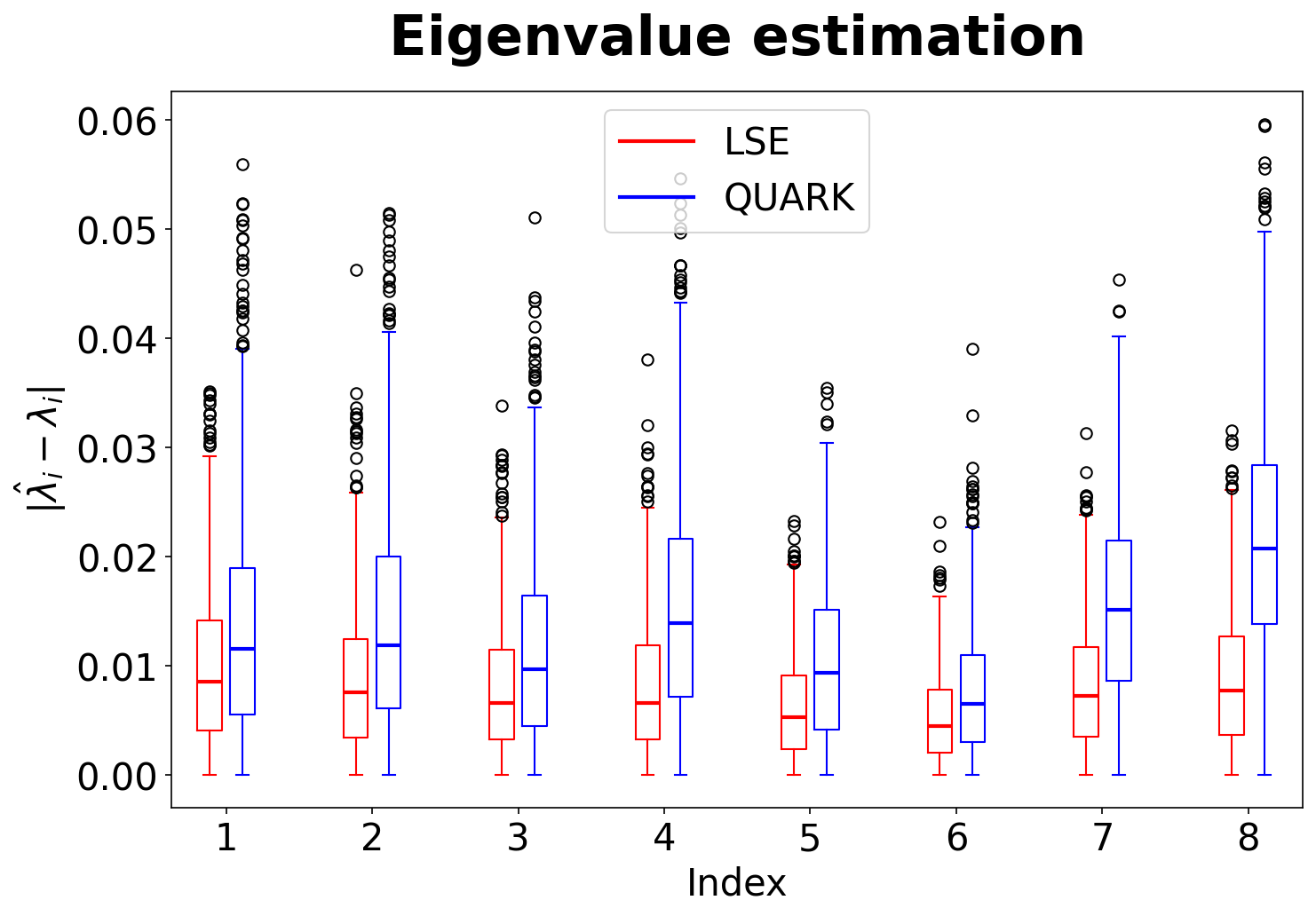
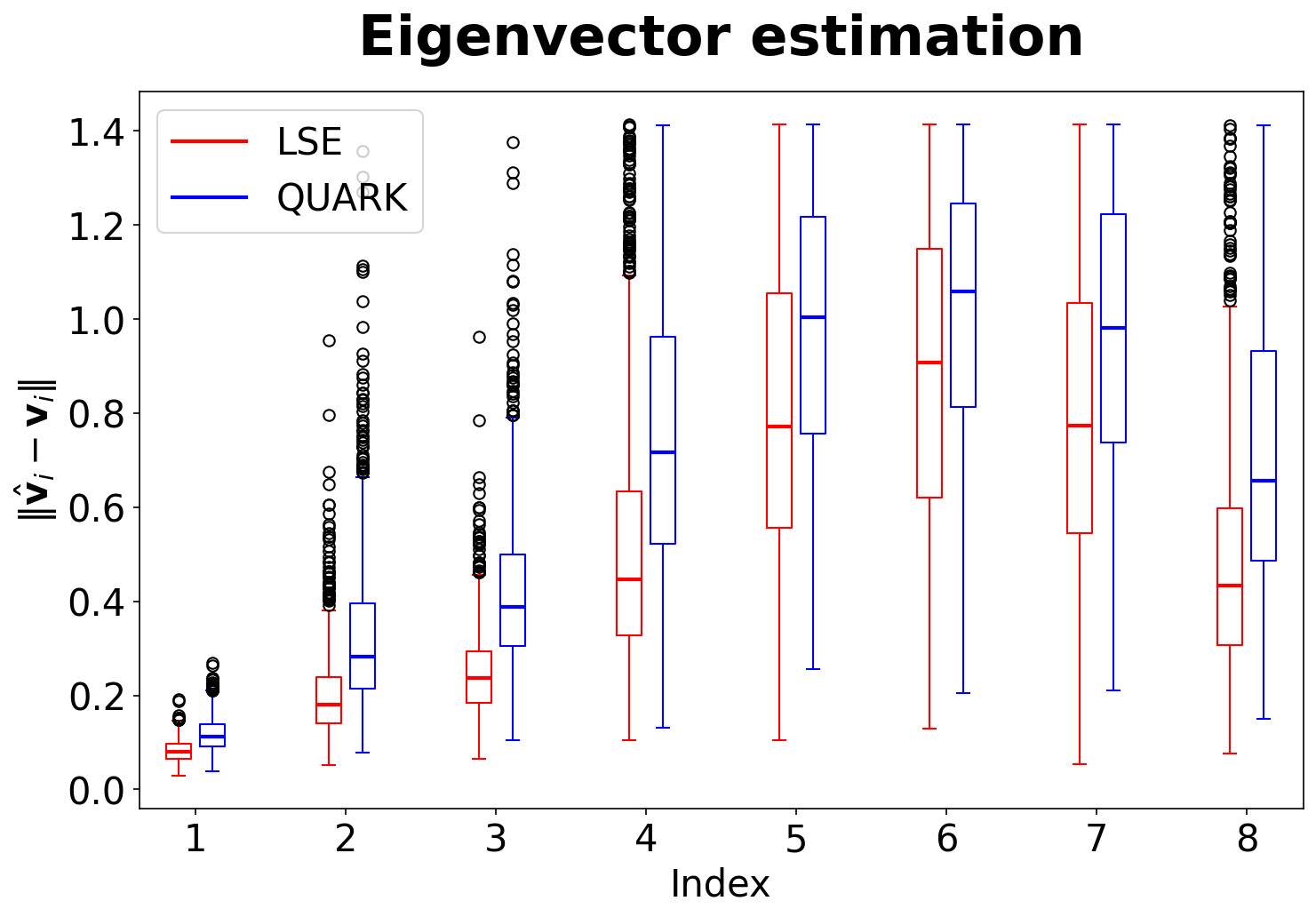
Refer to caption
Refer to caption
Figure 7: Spectral behavior of the LSE and QUARK estimator, based on 10001000 Monte Carlo repetitions with 𝔽=ℝ\mathbb{F}=\mathbb{R}. The boxplots are ordered by decreasing eigenvalue magnitude. Left: Absolute eigenvalue errors |λ^iLSE−λi||\hat{\lambda}^{\text{LSE}}_{i}-\lambda_{i}| (red) and |λ^iK−λi||\hat{\lambda}^{K}_{i}-\lambda_{i}| (blue). Right: Absolute eigenvector errors ‖𝐯^iLSE−𝐯i‖\|\hat{\mathbf{v}}^{\text{LSE}}_{i}-\mathbf{v}_{i}\| (red) and ‖𝐯^iK−𝐯i‖\|\hat{\mathbf{v}}_{i}^{K}-\mathbf{v}_{i}\| (blue).

Asymptotic Performances. As in Section 5.1, we vary the number of samples per observable rr increases. We perform the reconstructions for the LSE and various QUARK estimators. We then compare the results to the theoretical MSE under an exact unitary design. Note that since 𝒬=ℝ8\mathcal{Q}=\mathbb{R}^{8}, the damping factor satisfies α𝒬=1/5\alpha_{\mathcal{Q}}=1/5. Similar phenomenon is observed as in Section 5.1: The empirical behavior of the LSE closely follows the theoretical scaling. While all QUARK estimators exhibit larger errors asymptotically in comparison to the LSE estimator, the errors get closer to the theoretical LSE bound as cc increases. Nonetheless, Fig. 8 validates the asymptotic O​(r−1)O(r^{-1}) decay predicted by the theory.

Refer to caption
Figure 8: Asymptotic performances in terms of MSE of the LSE and various QUARK estimators with 𝔽=ℝ\mathbb{F}=\mathbb{R}.