Error estimates for tamed Euler and Randomized Euler schemes for SDEs with locally Lipschitz drift with applications to non-logconcave sampling and optimization

Iosif Lytras^† Archimedes, Athena Research Center, Greece and National Technical University of Athens, Athens,Greece. i.lytras@athenarc.gr and Angelos Ntousis^∗ ^∗ Archimedes, Athena Research Center, Greece aggelosntousis02@gmail.com

Abstract.

In this paper, we study the numerical discretization of stochastic differential equations with locally Lipschitz, super-linearly growing drift, and the resulting implications for sampling from non-log-concave distributions satisfying a logarithmic Sobolev inequality. In this regime, the classical Euler–Maruyama scheme underlying the unadjusted Langevin algorithm (ULA) is known to be unstable. We analyze the KL-accelerated tamed unadjusted Langevin algorithm (kTULA) and introduce a new tamed randomized midpoint scheme, termed tRLMC. Building on the shifted-composition approach of [5], we develop two new local-error frameworks that yield finite-time, non-asymptotic error estimates against the underlying SDE—in KL divergence for kTULA, and in total variation for tRLMC —valid for general locally Lipschitz drift. Specializing these frameworks to the sampling problem under a logarithmic Sobolev inequality, we obtain a near-optimal $\widetilde{O}(\varepsilon^{-1/2})$ iteration complexity for kTULA in KL divergence, with corresponding guarantees in total variation and Wasserstein distance. We further establish, for the first time, a non-asymptotic guarantee in total variation for a tamed randomized Langevin scheme under super-linear drift growth, together with the corresponding Wasserstein-distance bound, both with $\widetilde{O}(\varepsilon^{-1})$ complexity for tRLMC. As a consequence, both schemes yield non-asymptotic bounds for a non-convex excess-risk optimization problem.

1. Introduction

The numerical discretization of stochastic differential equations (SDEs) with super-linearly growing drift has attracted considerable attention in the numerical analysis of stochastic dynamics. Beyond its intrinsic interest, this analysis underpins a wide range of sampling algorithms used in computational statistics, Bayesian inference, and large-scale optimization. The general SDE of interest in this work takes the form

dX_{t}=-h(X_{t})\,dt+\sigma\,dB_{t},

(SDE)

where $h:\mathbb{R}^{d}\to\mathbb{R}^{d}$ is a locally Lipschitz drift that may grow super-linearly at infinity, $\sigma>0$ is a constant volatility, and $(B_{t})_{t\geq 0}$ is a canonical Wiener process in $\mathbb{R}^{d}$ with unit covariance. A canonical application consists of sampling from a target distribution $\pi$ on $\mathbb{R}^{d}$ , typically expressed in Gibbs form as $\pi(x)\propto e^{-\beta u(x)}$ for some potential function $u:\mathbb{R}^{d}\to\mathbb{R}$ . Under suitable assumptions on $u$ , this distribution arises as the invariant measure of the Langevin SDE

dX_{t}=-\nabla u(X_{t})\,dt+\sqrt{\tfrac{2}{\beta}}\,dB_{t},

(LSDE)

which is precisely (SDE) specialized to $h:=\nabla u$ and $\sigma:=\sqrt{2/\beta}$ . Motivated by this fundamental property of (LSDE), one of the most widely used algorithmic schemes for sampling from $\pi$ is the unadjusted Langevin algorithm (ULA), given recursively by

\theta^{\mathrm{ULA}}_{0}:=\theta_{0},\qquad\theta^{\mathrm{ULA}}_{n+1}=\theta^{\mathrm{ULA}}_{n}-\lambda\,h\!\left(\theta^{\mathrm{ULA}}_{n}\right)+\sqrt{\tfrac{2\lambda}{\beta}}\,\xi_{n+1},\qquad n\in\mathbb{N}_{0},

(ULA)

where $\theta_{n}\in\mathbb{R}^{d}$ , $n=1,2,\ldots$ , denotes the state variable of the algorithm, $(\xi_{n})_{n\geq 1}$ is an independent and identically distributed (i.i.d.) sequence of standard $d$ -dimensional random vectors with unit covariance, $\lambda>0$ is a step-size parameter, and $h:=\nabla u$ denotes the gradient of the potential $u$ . The guiding idea behind (ULA) is that it may be viewed as an Euler–Maruyama discretization of (LSDE), so that, for sufficiently large $n$ and sufficiently small $\lambda$ , $\theta^{\mathrm{ULA}}_{n}$ is distributed approximately according to the invariant measure of (LSDE), which is precisely the target distribution $\pi$ .

This connection has motivated a substantial literature devoted to establishing non-asymptotic convergence guarantees for (ULA) in various probability metrics, most notably Wasserstein distances, total variation, and information-theoretic divergences such as the Kullback–Leibler (KL) divergence. Much of this literature focuses on the case where $\pi$ is log-concave and the gradient $\nabla u$ is globally Lipschitz, corresponding respectively to convexity and smoothness of the potential $u$ ; see, e.g., [8, 9, 10] and references therein.

Beyond the globally Lipschitz log-concave setting, a substantial body of work has sought to relax convexity and smoothness assumptions on $u$ , notably through dissipativity, convexity-at-infinity, and related structural conditions; see, for instance, [7, 24, 6, 27]. A complementary line of research, initiated by the insights of Vempala and Wibisono [31], establishes convergence under isoperimetric inequalities, such as Poincaré and logarithmic Sobolev inequalities; see [11, 12, 6, 25].

This work examines the numerical discretization of (SDE) in a regime that lies at the intersection of two well-studied directions: relaxing global Lipschitz assumptions on the drift, and—in the sampling specialization—weakening convexity via isoperimetric inequalities. While each of these settings has been analyzed extensively in isolation, rigorous non-asymptotic guarantees in their combination—particularly in the presence of super-linear drift growth—remain limited in the literature. Crucially, the numerical-analytic obstacles arising from super-linear drift are not specific to the gradient case $h=\nabla u$ : explosion of moments, divergence of Euler–Maruyama in mean-square sense, and breakdown of standard local-error frameworks all occur at the level of (SDE), prompting a treatment that is general at the level of the SDE and only later specialized to sampling. This motivates the following two-fold question:

How does one derive finite-time error estimates for numerical discretizations of SDEs with super-linearly growing locally Lipschitz drift, and what guarantees can such estimates yield for sampling and optimization in the absence of log-concavity and global smoothness?

This scenario presents substantial challenges. As noted in several prior studies, both (ULA) and its stochastic variants, such as SGLD, may become unstable in such regimes. In particular, when $h$ grows super-linearly, the associated Euler–Maruyama scheme—which forms the backbone of (ULA)—can fail dramatically. A pivotal result in [12] showed that, in such cases, the numerical approximation may diverge from the true SDE solution in mean-square sense, even over finite time horizons. This phenomenon is directly linked to the explosion of moments in the discretized process, highlighting why standard schemes may break down when applied to approximate (SDE) with super-linearly growing drift $h$ .

Addressing this issue requires a fundamentally different approach—one that revisits the way in which (ULA) is designed as a numerical discretization of (LSDE), and leverages insights from the theory of numerical methods for SDEs. In this vein, a promising class of techniques—known as tamed Euler schemes—emerged in [13, 28, 29]. These methods modify the drift $h$ in order to ensure the stability of (ULA) even under super-linear growth. Specifically, they replace the original coefficient $h$ with a modified version $h_{\lambda}$ , depending on the stepsize $\lambda$ , which is constructed to satisfy two essential properties:

(P1)

The tamed coefficient $h_{\lambda}$ grows at most linearly, i.e., $h_{\lambda}(\theta)=O(\|\theta\|)$ as $\|\theta\|\to\infty$ .
(P2)

$h_{\lambda}$ converges pointwise to the original coefficient $h$ as $\lambda\to 0$ .

These properties ensure both the stability of the numerical scheme and consistency with the original dynamics as the stepsize vanishes.

Tamed Euler algorithms. In the context of Langevin-based sampling, taming techniques have been applied under strong dissipativity or convexity assumptions [3, 15, 23], in stochastic-gradient settings [19, 17], under a “convexity at infinity” assumption [26], and more recently under functional inequalities [21, 20, 22]. In parallel, truncated or projected schemes have been examined under logarithmic Sobolev assumptions [34].

In this work, we build on the KL-accelerated tamed unadjusted Langevin algorithm (kTULA) introduced in [22], which can be viewed as a modification of TULA designed to ensure stability under super-linear drift growth. The key idea underlying our analysis is that taming induces state-dependent perturbations in the dynamics, which fall outside the scope of existing KL frameworks. By explicitly controlling these perturbations, we establish non-asymptotic finite-time error estimates for kTULA in KL divergence under polynomial smoothness and dissipativity of the drift; when specialized to the sampling setting $h=\nabla u$ under a logarithmic Sobolev inequality, this yields improved convergence rates toward $\pi_{\beta}$ even in the presence of super-linear gradient growth.

Tamed randomized Euler algorithms. At the same time, an alternative line of work has focused on randomized discretization schemes for Langevin dynamics, where randomness is introduced directly at the level of the numerical integrator, for instance through randomized time steps or intermediate evaluations of the drift. Such methods have been shown to improve stability properties, reduce discretization bias, and, in certain regimes, achieve improved convergence rates compared to their deterministic counterparts.

A representative example, in the Langevin case $h=\nabla u$ , is the randomized midpoint Langevin algorithm, given by

	$\displaystyle Y_{n+1}^{\tau}$	$\displaystyle=Y_{n}-\tau_{n+1}\nabla u(Y_{n})\,\lambda+\sqrt{2}\,\Delta W_{n+1}^{\tau},\qquad Y_{0}=x_{0},$
	$\displaystyle Y_{n+1}$	$\displaystyle=Y_{n}-\nabla u(Y_{n+1}^{\tau})\,\lambda+\sqrt{2}\,\Delta W_{n+1},\qquad n\in\mathbb{N}_{0},$

where $(\tau_{n})_{n\in\mathbb{N}}$ are i.i.d. uniform random variables on $[0,1]$ .

Originally introduced as numerical methods for SDEs with irregular coefficients, such randomized schemes were later adapted to sampling settings in [30] and further developed in [4, 36, 5, 16]. In the context of sampling, randomized discretizations are particularly appealing, as they can better capture the underlying stochastic dynamics while mitigating the accumulation of discretization error.

However, existing analyses of these methods rely crucially on global Lipschitz assumptions on the gradient. In particular, it remains unclear whether the stability and bias-reduction properties of randomized schemes persist when the drift exhibits super-linear growth, as is typical in non-log-concave and high-dimensional learning problems.

Motivated by the developments in both the randomized Euler and tamed Euler literature, it is natural to investigate whether the stabilizing effect of taming can be combined with the robustness properties of randomized discretizations. This raises the question of whether one can construct discretization schemes that remain stable under super-linear drift growth while retaining the favorable bias properties of randomized methods.

In this work, we address this question by introducing and analyzing a tamed randomized Langevin Monte Carlo algorithm (tRLMC). We establish non-asymptotic finite-time error estimates for this method in total variation against the underlying SDE, and, in the sampling specialization, derive non-asymptotic convergence guarantees in non-log-concave regimes, including explicit bounds in Wasserstein distance and total variation, with further implications for optimization.

Our contributions. Our results are organized in two layers: finite-time error estimates against the underlying (SDE), valid for general locally Lipschitz drift, and their specialization to the sampling problem under $h=\nabla u$ and a logarithmic Sobolev inequality. The two finite-time frameworks address complementary settings: the KL framework applies to the deterministic tamed Euler scheme, where a sharp cross-regularity estimate is available, whereas the TV framework applies to the randomized scheme, for which such a cross-regularity estimate is currently out of reach due to the randomization of the integration time.

(i)

Finite-time KL error estimates for SDEs with locally Lipschitz drift. Building on [5], we develop a new local-error framework for controlling the KL divergence between a discretization scheme and the (SDE) when the drift grows super-linearly. Applied to (kTULA), the framework yields a finite-time estimate of the form

\mathrm{KL}\!\bigl(\mu\widehat{P}^{N}\,\big\|\,\nu P^{N}\bigr)\;\lesssim\;\tfrac{1}{\lambda}\,\mathcal{W}_{2}^{2}(\mu,\nu)\;+\;\bigl((N\lambda)\vee\log N\bigr)\,\lambda^{2},

valid for general locally Lipschitz drift; see Theorem 1.

(ii)

Finite-time TV error estimates for randomized schemes under super-linear drift. By combining the taming methodology with a randomized midpoint method, we introduce a new discretization, termed tRLMC, and develop a corresponding total variation local-error framework. This yields the first finite-time error estimate in total variation for a randomized scheme applied to SDEs with super-linearly growing locally Lipschitz drift; see Theorem 2.
(iii)

Near-optimal sampling guarantees for tamed Euler schemes in $\mathrm{KL}$ divergence. Specializing the KL framework to the Langevin case $h=\nabla u$ under a logarithmic Sobolev inequality, we derive an explicit $\tilde{O}(\epsilon^{-\frac{1}{2}})$ complexity bound for kTULA to reach accuracy $\epsilon$ in KL divergence toward $\pi_{\beta}$ . This further yields improved guarantees in Wasserstein and total variation distances.
(iv)

Sampling guarantees for tamed randomized schemes. Specializing the TV framework to the Langevin case, we show that tRLMC achieves $\tilde{O}(\epsilon^{-1})$ complexity for sampling toward $\pi_{\beta}$ in $W_{2}$ and total variation distance under a logarithmic Sobolev inequality.

(v)

Connection with optimization. We apply our Wasserstein convergence results to obtain explicit non-asymptotic excess-risk bounds for tamed Langevin schemes in the non-log-concave setting. More precisely, we decompose the excess risk as:

\underbrace{\mathbb{E}\!\bigl[u(\theta_{n})\bigr]-\mathbb{E}_{\pi_{\beta}}\!\bigl[u(x)\bigr]}_{\text{sampling error}}+\underbrace{\mathbb{E}_{\pi_{\beta}}\!\bigl[u(x)\bigr]-u^{*}}_{\text{concentration for large }\beta},

where $\theta_{n}$ denotes the $n$ -th iterate of the algorithm. Thus, a solution to the sampling problem yields corresponding optimization guarantees for sufficiently large $\beta$ .

Organization of the paper. The remainder of the paper is organized as follows. Section 2 introduces the necessary notation, the structural assumptions on the drift of (SDE), and the functional inequalities used in the sampling specialization. Section 3 introduces the two tamed schemes (kTULA) and (tRLMC) and presents the main finite-time error estimates against the underlying SDE in KL divergence and total variation, together with their specialization to sampling in KL, total variation, and Wasserstein distance, and the resulting implications for optimization. Section 4 reports numerical experiments illustrating the stabilizing effect of taming both for sampling and for a nonlinear optimization problem. Section 5 presents the new local-error frameworks underlying our analysis, including the KL framework for kTULA, the corresponding TV framework for the randomized scheme, and the Wasserstein convergence argument for tRLMC. Detailed proofs of all auxiliary results and of the main theorems are deferred to Appendices A-D.

2. Preliminaries and Blanket Assumptions

In this section, we provide the necessary groundwork for stating the proposed algorithmic schemes and our main results. We adopt throughout a two-layer convention: structural assumptions and notation are formulated at the level of the general (SDE) with locally Lipschitz drift $h$ , while functional inequalities and the target measure $\pi_{\beta}$ are introduced only in the sampling specialization $h=\nabla u$ .

2.1. Notation

Throughout, $\|\cdot\|$ denotes the Euclidean norm on $\mathbb{R}^{d}$ and $\langle\cdot,\cdot\rangle$ its associated inner product. For a sufficiently smooth function $f:\mathbb{R}^{d}\to\mathbb{R}$ , we write $\nabla f$ , $\nabla^{2}f$ and $\Delta f$ for its gradient, Hessian matrix, and Laplacian respectively. For a continuously differentiable map $F:\mathbb{R}^{d}\to\mathbb{R}^{d}$ , we write $J(F)$ for its Jacobian. In the gradient case $F=\nabla u$ , one has $J(\nabla u)=\nabla^{2}u$ . For a measurable map $T$ , we write $\operatorname{Law}(T)$ for its induced distribution. For a probability measure $\mu$ and Markov kernel $P$ , the pushforward measure $\mu P$ is

(\mu P)(A):=\int_{\mathbb{R}^{d}}P(x,A)\,\mu(dx),\qquad\mu P^{n}:=\mu\underbrace{P\cdots P}_{n\ \text{times}}.

SDE semigroup and one-step kernel. Let $(P_{t})_{t\geq 0}$ denote the Markov semigroup of (SDE), i.e., $P_{t}(x,\cdot)=\operatorname{Law}(X_{t}^{x})$ where $X_{0}^{x}=x$ . Fix a step size $\lambda>0$ and define the one-step diffusion kernel

P:=P_{\lambda}.

In the sampling specialization $h=\nabla u$ , $(P_{t})_{t\geq 0}$ coincides with the Langevin semigroup of (LSDE).

2-Wasserstein distance. Let $\mathcal{P}_{2}(\mathbb{R}^{d})$ denote the space of probability measures with finite second moment. For $\mu,\nu\in\mathcal{P}_{2}(\mathbb{R}^{d})$ , the $2$ -Wasserstein distance is defined by

\mathcal{W}_{2}(\mu,\nu):=\left(\inf_{\gamma\in\mathcal{C}(\mu,\nu)}\int_{\mathbb{R}^{d}\times\mathbb{R}^{d}}\|x-y\|^{2}\,\gamma(dx,dy)\right)^{1/2},

(1)

where $\mathcal{C}(\mu,\nu)$ denotes the set of couplings of $\mu$ and $\nu$ , that is, probability measures on $\mathbb{R}^{d}\times\mathbb{R}^{d}$ with marginals $\mu$ and $\nu$ . Equivalently, $(X,Y)$ is a coupling of $\mu$ and $\nu$ if $\operatorname{Law}(X)=\mu$ and $\operatorname{Law}(Y)=\nu$ .

Kullback–Leibler divergence. Let $\mathcal{P}(\mathbb{R}^{d})$ denote the space of probability measures on $\mathbb{R}^{d}$ . For $\mu,\nu\in\mathcal{P}(\mathbb{R}^{d})$ , the Kullback–Leibler divergence is defined by

\mathrm{KL}(\mu\|\nu):=\int_{\mathbb{R}^{d}}\log\!\left(\frac{d\mu}{d\nu}\right)\,d\mu,

(2)

whenever $\mu$ is absolutely continuous with respect to $\nu$ , and $\mathrm{KL}(\mu\|\nu):=+\infty$ otherwise.

We rely on the standard chain rule and data processing inequality for relative entropy, which yield the marginal bound $\mathrm{KL}(\mu^{Y}\|\nu^{Y})\leq\mathrm{KL}(\mu^{X,Y}\|\nu^{X,Y})$ . A key refinement for our purposes is the shifted chain rule [5]. By introducing an auxiliary variable $X^{\prime}$ , it provides the flexible bound

\mathrm{KL}(\mu^{Y}\|\nu^{Y})\leq\mathrm{KL}(\mu^{X^{\prime}}\|\nu^{X})+\inf_{\gamma\in\mathcal{C}(\mu^{X},\mu^{X^{\prime}})}\int\mathrm{KL}\!\bigl(\mu^{Y|X=x}\,\big\|\,\nu^{Y|X=x^{\prime}}\bigr)\,\gamma(dx,dx^{\prime}).

(3)

This freedom to couple $X$ and $X^{\prime}$ is central to the shifted comparison arguments developed in Section 5.

Rényi divergence. The Rényi divergence of order $q>1$ between two probability measures $\mu,\nu$ is defined by

\mathsf{R}_{q}(\mu\|\nu):=\frac{1}{q-1}\log\int\left(\frac{d\mu}{d\nu}\right)^{q}\,d\nu,

(4)

whenever $\mu\ll\nu$ , and $+\infty$ otherwise. In the limit as $q\to 1$ , this recovers the Kullback–Leibler divergence, while the case $q=2$ yields $\mathsf{R}_{2}=\log(1+\chi^{2})$ , where $\chi^{2}$ is the chi-squared divergence.

Infinitesimal generator. We denote by $\mathcal{L}$ the infinitesimal generator of (SDE),

\mathcal{L}f\;:=\;\tfrac{\sigma^{2}}{2}\,\Delta f\;-\;\langle h,\nabla f\rangle,

which, in the sampling specialization $h=\nabla u$ and $\sigma=\sqrt{\frac{2}{\beta}}$ , reduces to the Langevin generator $\mathcal{L}f=\tfrac{1}{\beta}\Delta f-\langle\nabla u,\nabla f\rangle$ .

2.2. Assumptions on the drift

We impose the following structural conditions on the drift $h$ of (SDE).

(A1)

Polynomial Jacobian growth. There exist constants $L>0$ and $\ell\geq 0$ such that

$\max\bigl\{\|h(x)\|,\ \|J(h)(x)\|\bigr\}\leq L\bigl(1+\|x\|^{2\ell}\bigr),\qquad\forall x\in\mathbb{R}^{d}.$

(A2)

Polynomial Lipschitz continuity. There exist constants $L^{\prime}>0$ and $\ell^{\prime}\geq 0$ such that

\|h(x)-h(y)\|\leq L^{\prime}\bigl(1+\|x\|+\|y\|\bigr)^{\ell^{\prime}}\|x-y\|,\qquad\forall x,y\in\mathbb{R}^{d}.

(A3)

One-sided Lipschitz continuity. There exists a constant $K^{\prime}\in\mathbb{R}$ such that

$\langle h(x)-h(y),\,x-y\rangle\geq-K^{\prime}\|x-y\|^{2},\qquad\forall x,y\in\mathbb{R}^{d}.$
(A4)

Dissipativity. There exist constants $a,b>0$ such that

$\langle h(x),x\rangle\geq a\|x\|^{2}-b,\qquad\forall x\in\mathbb{R}^{d}.$

(A5)

Polynomial Jacobian Lipschitz continuity. There exist constants $L^{\prime\prime}>0$ and $\ell^{\prime\prime}\geq 0$ such that

\|J(h)(x)-J(h)(y)\|\leq L^{\prime\prime}(1+\|x\|+\|y\|)^{\ell^{\prime\prime}}\|x-y\|,\qquad\forall x,y\in\mathbb{R}^{d}.

Assumption (A1) allows the drift and its Jacobian to grow polynomially at infinity, thereby encompassing a wide class of drift coefficients with super-linear growth that fall outside the scope of the standard global Lipschitz framework. In the sampling specialization $h=\nabla u$ , it covers non-convex potentials for which classical convergence analyses of (ULA) are not directly applicable.

Assumption (A2) ensures that the drift is locally Lipschitz continuous, with a Lipschitz modulus that may itself grow polynomially. This condition is substantially weaker than global Lipschitz continuity and is compatible with super-linear drifts, while still being sufficient to establish well-posedness of (SDE) and stability of the numerical schemes considered in this work.

Assumption (A3) is a one-sided Lipschitz condition, which plays a key role in controlling the propagation of errors between coupled trajectories of (SDE). It is strictly weaker than monotonicity or strong convexity, and is particularly well suited to the analysis of non-convex dynamics.

Assumption (A4) is a dissipativity condition that ensures coercive behavior of the drift at infinity. This assumption is central to our analysis, as it allows us to derive uniform-in-time moment bounds for both (SDE) and its discretizations, and is a natural coercivity-type condition in applications.

Assumption (A5) is imposed only in the analysis of the (kTULA) scheme. It provides the additional Jacobian regularity—namely, local Lipschitz continuity of $J(h)$ with polynomial modulus—required to obtain the improved weak error rate underlying our KL convergence bounds. In the gradient case $h=\nabla u$ , since $J(h)=\nabla^{2}u$ , this reduces to a polynomial-Lipschitz Hessian condition on the potential. The assumption is not needed for the randomized scheme (tRLMC), whose bias-reduction mechanism does not rely on second-order smoothness of the drift.

2.3. Sampling and functional inequalities

We now turn to the specialization of (SDE) that underlies the sampling application. Throughout this subsection and whenever sampling guarantees are stated, we assume that $h=\nabla u$ for some $u:\mathbb{R}^{d}\to\mathbb{R}$ satisfying $\int_{\mathbb{R}^{d}}e^{-\beta u(x)}\,dx<\infty$ for any $\beta>0$ , and we set $\sigma=\sqrt{\frac{2}{\beta}}$ . Under this specialization, (SDE) reduces to (LSDE), which admits as invariant measure the Gibbs distribution

\pi_{\beta}(A)\;:=\;\frac{\int_{A}e^{-\beta u(x)}\,dx}{\int_{\mathbb{R}^{d}}e^{-\beta u(x)}\,dx},\qquad A\in\mathcal{B}(\mathbb{R}^{d}).

In addition to the structural assumptions (A1)–(A5) on $h=\nabla u$ , we impose a functional inequality on $\pi_{\beta}$ .

(A6)

Logarithmic Sobolev inequality (LSI). The target distribution $\pi_{\beta}$ satisfies a logarithmic Sobolev inequality with constant $C_{\mathrm{LSI}}>0$ , meaning that for every probability measure $\nu\ll\pi_{\beta}$ with density $f:=\frac{d\nu}{d\pi_{\beta}}$ ,

\mathrm{KL}(\nu\|\pi_{\beta})=\int_{\mathbb{R}^{d}}f\log f\,d\pi_{\beta}\leq\frac{1}{2C_{\mathrm{LSI}}}\,I_{\pi_{\beta}}(\nu),

(LSI)

where $I_{\pi_{\beta}}(\nu)$ denotes the relative Fisher information of $\nu$ with respect to $\pi_{\beta}$ .

Assumption (A6) is widely used in the analysis of Langevin dynamics since it implies exponential ergodicity in relative entropy. In particular, by the Bakry–Émery theorem [1], (LSI) holds for strongly convex potentials and is stable under bounded perturbations, Lipschitz mappings, and convolutions.

Finally, (LSI) implies Talagrand’s transportation-cost inequality: for every $\nu\in\mathcal{P}_{2}(\mathbb{R}^{d})$ ,

\mathcal{W}_{2}(\nu,\pi_{\beta})\;\leq\;\sqrt{\frac{2}{C_{\mathrm{LSI}}}\,\mathrm{KL}(\nu\|\pi_{\beta})}.

(TI)

3. Tamed schemes and main results

This section introduces the two tamed discretization schemes analyzed in this work—(kTULA) and (tRLMC)—and presents the corresponding main results. The results in this section are organized into two distinct layers. First, we establish finite-time error estimates against the underlying (SDE), which rely solely on the structural assumptions (A1)–(A5) for the general drift $h$ . Second, we derive sampling and optimization guarantees toward $\pi_{\beta}$ , which additionally invoke the gradient specialization $h=\nabla u$ and Assumption (A6).

3.1. Tamed discretizations

Throughout this subsection, we fix constants $a>0$ and $\ell\geq 0$ , and define, for each $\lambda>0$ , the tamed drift $h_{\lambda}:\mathbb{R}^{d}\to\mathbb{R}^{d}$ associated with $h$ by

h_{\lambda}(x):=ax+\frac{h(x)-ax}{\bigl(1+\lambda\|x\|^{2(\ell+1)}\bigr)^{1/2}}.

(4)

The construction (4) is well defined for any locally Lipschitz drift $h$ and does not require $h$ to be a gradient field.

The kTULA scheme. The KL-accelerated tamed unadjusted Langevin algorithm is given by

\widehat{X}_{0}^{\lambda}:=X_{0},\qquad\widehat{X}_{n+1}^{\lambda}=\widehat{X}_{n}^{\lambda}-\lambda\,h_{\lambda}(\widehat{X}_{n}^{\lambda})+\sqrt{\frac{2\lambda}{\beta}}\,\xi_{n+1},\qquad n\in\mathbb{N}_{0},

(kTULA)

where $X_{0}$ is an $\mathbb{R}^{d}$ -valued random variable, $\lambda>0$ is the stepsize, $\beta>0$ is the inverse temperature, and $(\xi_{n})_{n\in\mathbb{N}_{0}}$ are i.i.d. standard $d$ -dimensional Gaussian random vectors. We denote by $\pi_{n}^{\lambda}$ the density of $\operatorname{Law}(\widehat{X}_{n}^{\lambda})$ for all $n\in\mathbb{N}_{0}$ .

Remark 1.

The design of the tamed coefficient $h_{\lambda}$ in (4) follows from that of mTULA [26] and sTULA [20]. It allows us to derive several properties of $h_{\lambda}$ , which are crucial to establish moment estimates and convergence results of (kTULA). More precisely, by adopting the splitting trick originally used in [20], the tamed coefficient $h_{\lambda}$ satisfies a dissipativity condition, which enables contraction of the algorithm (kTULA) and therefore an easier computation of the associated moment bounds. Moreover, dividing by the term $\bigl(1+\lambda\|x\|^{2(\ell+1)}\bigr)^{1/2}$ in (4) yields an improved upper bound for the difference between $h_{\lambda}$ and $h$ , compared to [20].

Main results. Denote by

\lambda_{\max}^{\mathrm{kTULA}}:=\min\left\{1,\;\frac{1}{8a},\;\frac{1}{(6L_{0})^{2}}\right\},

(5)

where $L_{0}:=2a+4L+(\ell+1)(2L+a)$ .

Throughout this subsection, for a fixed step size $\lambda>0$ , we write $P:=P_{\lambda}$ for the one-step kernel of (SDE) run for time $\lambda$ , and $\widehat{P}$ for the one-step kernel associated with (kTULA).

3.1.1. Finite-time KL error estimate against the underlying SDE

Our first result is a finite-time KL error estimate between (kTULA) and (SDE), valid for general locally Lipschitz drift.

Theorem 1 (KL local-error bound for kTULA).

Assume (A1)–(A5). Let $\lambda\in(0,\lambda_{\max}^{\mathrm{kTULA}}]$ . Then there exist constants $C_{1},C>0$ , depending at most polynomially on the dimension and independent of $N$ and $\lambda$ , such that for all $\mu,\nu\in\mathcal{P}_{2}(\mathbb{R}^{d})$ and all $N\in\mathbb{N}$ with $N\geq 3$ ,

\mathrm{KL}\!\bigl(\mu\,\widehat{P}^{N}\,\big\|\,\nu\,P^{N}\bigr)\;\leq\;C_{1}\,\frac{1}{\lambda}\,\mathcal{W}_{2}^{2}(\mu,\nu)\;+\;C\,\bigl((N\lambda)\vee\log N\bigr)\lambda^{2}.

(6)

Remark 2.

In particular, for $\mu=\nu$ and $N\geq 3$ , the Wasserstein term vanishes, and

\mathrm{KL}\!\bigl(\mu\,\widehat{P}^{N}\,\big\|\,\mu\,P^{N}\bigr)\;\leq\;C\,\bigl((N\lambda)\vee\log N\bigr)\lambda^{2}.

3.1.2. Sampling specialization

We now specialize Theorem 1 to the sampling setting introduced in Section 2.3. From here on through the end of this subsection, we assume $h=\nabla u$ , so that (LSDE) admits $\pi_{\beta}$ as its invariant measure, and we additionally impose the logarithmic Sobolev inequality (A6). Under this specialization, the kernel $P$ becomes the one-step Langevin diffusion kernel of (LSDE), and Theorem 1 combined with the exponential ergodicity of $(P_{t})_{t\geq 0}$ yields sampling guarantees toward $\pi_{\beta}$ .

Corollary 1 (KL sampling guarantee for kTULA under LSI).

Assume (A1)–(A6), and let $\lambda\in(0,\lambda_{\max}^{\mathrm{kTULA}}]$ . Then there exist constants $C_{1},C>0$ such that, for all $\mu\in\mathcal{P}_{2}(\mathbb{R}^{d})$ and all $N\geq 3$ ,

\mathrm{KL}\!\bigl(\mu\widehat{P}^{N}\,\big\|\,\pi_{\beta}\bigr)\leq\mathrm{KL}\!\bigl(\mu\widehat{P}^{N}\,\big\|\,\mu P^{N}\bigr)+R_{2}\!\bigl(\mu P^{N}\,\big\|\,\pi_{\beta}\bigr),

(7)

where $R_{2}(\cdot\|\cdot)$ denotes the Rényi divergence of order $2$ . Consequently,

\mathrm{KL}\!\bigl(\mu\widehat{P}^{N}\,\big\|\,\pi_{\beta}\bigr)\leq C\,\bigl((N\lambda)\vee\log N\bigr)\lambda^{2}+e^{-2C_{\mathrm{LSI}}N\lambda}\,R_{2}\!\bigl(\mu\,\big\|\,\pi_{\beta}\bigr).

(8)

We next deduce explicit mixing-time guarantees from this bound.

Proposition 1 (Mixing time in KL for kTULA under LSI).

Assume (A1)–(A6), and let $\lambda\in(0,\lambda_{\max}^{\mathrm{kTULA}}]$ . Fix $\mu\in\mathcal{P}_{2}(\mathbb{R}^{d})$ and assume $R_{0}:=R_{2}(\mu\|\pi_{\beta})<\infty$ . Then

\mathrm{KL}\!\bigl(\mu\,\widehat{P}^{N}\,\big\|\,\pi_{\beta}\bigr)\;\leq\;C\,\bigl((N\lambda)\vee\log N\bigr)\lambda^{2}\;+\;e^{-2C_{\mathrm{LSI}}N\lambda}\,R_{0}.

In particular, for $\lambda\leq\widetilde{O}(\sqrt{\varepsilon})$ , it suffices to take $N\geq\widetilde{O}\!\left(\frac{1}{\sqrt{\varepsilon}}\right)$ to ensure

\mathrm{KL}\!\bigl(\mu\,\widehat{P}^{N}\,\big\|\,\pi_{\beta}\bigr)\leq\varepsilon.

The KL bound further implies convergence in stronger metrics.

Corollary 2 (TV mixing time via Pinsker).

Assume the conditions of Corollary 1 and let $\lambda\in(0,\lambda_{\max}^{\mathrm{kTULA}}]$ . Fix $\mu\in\mathcal{P}_{2}(\mathbb{R}^{d})$ and assume $R_{0}:=R_{2}(\mu\|\pi_{\beta})<\infty$ . Then

TV(\mu\widehat{P}^{N},\pi_{\beta})\;\leq\;C\,\lambda\sqrt{(N\lambda)\vee\log N}\;+\;e^{-C_{\mathrm{LSI}}N\lambda}\sqrt{R_{0}}.

As a consequence, for $\lambda\leq\widetilde{O}(\varepsilon)$ , it suffices to take $N\geq\widetilde{O}(1/\varepsilon)$ to ensure

TV(\mu\widehat{P}^{N},\pi_{\beta})\leq\varepsilon.

Corollary 3 ( $W_{2}$ mixing time via Talagrand).

Assume the conditions of Corollary 1 and let $\lambda\in(0,\lambda_{\max}^{\mathrm{kTULA}}]$ . Fix $\mu\in\mathcal{P}_{2}(\mathbb{R}^{d})$ and assume $R_{0}:=R_{2}(\mu\|\pi_{\beta})<\infty$ . Then there exist constants $C_{W_{2}},c_{0}>0$ , where $C_{W_{2}}$ depends at most polynomially on the dimension and $c_{0}$ depends on $C_{\mathrm{LSI}}$ , such that

\mathcal{W}_{2}\!\bigl(\mu\widehat{P}^{N},\pi_{\beta}\bigr)\;\leq\;C_{W_{2}}\!\left(\lambda\sqrt{(N\lambda)\vee\log N}+e^{-c_{0}N\lambda}\right).

As a consequence, for $\lambda\leq\widetilde{O}(\varepsilon)$ , it suffices to take $N\geq\widetilde{O}(1/\varepsilon)$ to guarantee

\mathcal{W}_{2}\!\bigl(\mu\widehat{P}^{N},\pi_{\beta}\bigr)\leq\varepsilon.

Implications for optimization. When $\beta$ is sufficiently large, the Gibbs measure $\pi_{\beta}$ concentrates around the minimizers of $u$ [14]. As a result, (kTULA) may also be used to address the optimization problem

\operatorname*{minimize}\qquad\mathbb{R}^{d}\ni\theta\mapsto u(\theta).

Corollary 4 (Expected excess risk bound for kTULA).

Assume (A1)–(A6), and let $\lambda\in(0,\lambda_{\max}^{\mathrm{kTULA}}]$ . Let $(\widehat{X}_{n})_{n\geq 0}$ be the (kTULA) iterates. Fix $\mu:=\operatorname{Law}(\widehat{X}_{0})$ such that $R_{0}:=R_{2}(\mu\|\pi_{\beta})<\infty$ . Then there exist constants $C_{0},C_{1},C_{2},C_{3}>0$ , independent of $N$ and $\lambda$ , such that for all $N\in\mathbb{N}$ ,

\mathbb{E}\!\bigl[u(\widehat{X}_{N})\bigr]-\inf_{\theta\in\mathbb{R}^{d}}u(\theta)\;\leq\;C_{1}\,e^{-C_{0}N\lambda}+C_{2}\,\lambda\,\sqrt{(N\lambda)\vee\log N}+C_{3}\frac{\log\beta}{\beta}.

(9)

3.2. Tamed randomized discretization

In addition to the fully explicit (kTULA), we also consider a randomized midpoint discretization equipped with our taming scheme. This construction is designed to handle super-linearly growing drifts within the randomized framework, while preserving stability and consistency with the underlying (SDE).

Using this randomized midpoint construction, we define the tamed randomized Langevin Monte Carlo algorithm as follows:

	$\displaystyle\bar{Y}_{n+1}^{\tau}$	$\displaystyle=\bar{Y}_{n}-\lambda\,h_{\lambda}(\bar{Y}_{n})\,\tau_{n+1}+\sqrt{\tfrac{2}{\beta}}\,\Delta W_{n+1}^{\tau},\qquad\bar{Y}_{0}=x_{0},$		(tRLMC)
	$\displaystyle\bar{Y}_{n+1}$	$\displaystyle=\bar{Y}_{n}-\lambda\,h_{\lambda}(\bar{Y}_{n+1}^{\tau})+\sqrt{\tfrac{2}{\beta}}\,\Delta W_{n+1},\qquad n\in\mathbb{N}_{0}.$		(tRLMC)

Here, $(\tau_{n})_{n\geq 1}$ is an i.i.d. sequence of random variables uniformly distributed on $(0,1)$ , independent of the Brownian motion $W$ , and

\Delta W_{n+1}^{\tau}:=W_{t_{n}+\tau_{n+1}\lambda}-W_{t_{n}},\qquad\Delta W_{n+1}:=W_{t_{n+1}}-W_{t_{n}},

where $t_{n}=n\lambda$ for $n\in\mathbb{N}_{0}$ , and the tamed drift $h_{\lambda}$ is defined by (4).

Main results. Denote by

\lambda_{\max}^{\mathrm{tRLMC}}:=\min\Bigl\{1,\;\tfrac{1}{8a},\;\tfrac{a}{2CL_{0}^{2}},\;\bigl(\tfrac{pa}{4C_{p}}\bigr)^{2}\Bigr\},

(10)

where the constants are made explicit in the proof of Lemma 12.

Throughout this subsection, for a fixed step size $\lambda>0$ , we write $P:=P_{\lambda}$ for the one-step kernel of (SDE) run for time $\lambda$ , and $\widetilde{P}$ for the one-step kernel associated with (tRLMC).

3.2.1. Finite-time TV error estimate against the underlying SDE

Our main finite-time result for (tRLMC) is a total-variation error estimate against (SDE), valid for general locally Lipschitz drift.

Theorem 2 (TV local-error bound for tRLMC).

Assume (A1)–(A4) and let $\lambda\in(0,\lambda_{\max}^{\mathrm{tRLMC}}]$ . Then there exist constants $C_{1},C>0$ , independent of $N$ and $\lambda$ , such that for all $\mu,\nu\in\mathcal{P}_{2}(\mathbb{R}^{d})$ and all $N\in\mathbb{N}$ with $N\geq 3$ ,

TV\!\bigl(\mu\,\widetilde{P}^{N}\,\big\|\,\nu\,P^{N}\bigr)\;\leq\;C_{1}\,\frac{1}{\sqrt{\lambda}}\,\mathcal{W}_{2}(\mu,\nu)\;+\;C\lambda\sqrt{\,\bigl((N\lambda)\vee\log N\bigr)}.

(11)

Theorem 2 requires only (A1)–(A4)—in particular, it does not require the Jacobian regularity (A5) used in the KL framework—and is valid for general locally Lipschitz drift, with no gradient structure imposed on $h$ . To the best of our knowledge, this is the first finite-time total-variation error estimate for a randomized discretization scheme applied to SDEs with super-linearly growing drift.

3.2.2. Sampling specialization

We now specialize Theorem 2 to the sampling setting. From here on through the end of this subsection, we assume $h=\nabla u$ , so that (LSDE) admits $\pi_{\beta}$ as its invariant measure, and we additionally impose Assumption (A6).

Corollary 5 (TV mixing time for tRLMC).

Assume (A1)–(A6), and let $\lambda\in(0,\lambda_{\max}^{\mathrm{tRLMC}}].$ There holds

TV(\mu_{0}\widetilde{P}^{N},\pi_{\beta})\;\leq\;C\lambda\sqrt{\,\bigl((N\lambda)\vee\log N\bigr)}\;+\;\sqrt{e^{-C_{\mathrm{LSI}}\lambda N}\mathrm{KL}(\mu_{0}\,\|\,\pi_{\beta})}.

As a result, for $\lambda\leq\widetilde{O}({\varepsilon})$ one needs $N\geq\widetilde{O}\!\left(\frac{1}{\varepsilon}\right)$ to guarantee

TV(\mu_{0}\widetilde{P}^{N},\pi_{\beta})\leq\varepsilon.

We also obtain convergence bounds in Wasserstein distance.

Theorem 3 (Wasserstein convergence for tRLMC).

Assume (A1)–(A6), and let $\lambda\in(0,\lambda_{\max}^{\mathrm{tRLMC}}].$ There holds

W_{2}(\mu_{0}\widetilde{P}^{n},\pi_{\beta})\;\leq\;C_{W_{2}}\bigl(\lambda+e^{-c_{0}\lambda n}\bigr),

where $C_{W_{2}}$ depends polynomially on the dimension and $c_{0}$ depends on $C_{\mathrm{LSI}}$ . As a result, for $\lambda\leq\widetilde{O}({\varepsilon})$ one needs $N\geq\widetilde{O}\!\left(\frac{1}{\varepsilon}\right)$ to guarantee

W_{2}(\mu_{0}\widetilde{P}^{N},\pi_{\beta})\leq\varepsilon.

Implications for optimization. As for (kTULA), we connect the Wasserstein convergence bound to the optimization problem $\min_{\theta\in\mathbb{R}^{d}}u(\theta)$ via the concentration of $\pi_{\beta}$ around the minimizers of $u$ .

Corollary 6 (Expected excess risk bound for tRLMC).

Assume (A1)–(A6), and let $x_{n}$ be the $n$ -th iterate of the tamed randomized Langevin Monte Carlo scheme (tRLMC). There exist constants $C,C^{\prime},c_{0}>0$ , depending at most polynomially on the dimension, such that

\mathbb{E}[u(x_{n})]-u^{*}\;\leq\;C\bigl(\lambda+e^{-c_{0}\lambda n}\bigr)+C^{\prime}\frac{\log\beta}{\beta}.

3.3. Comparison with related literature

We compare our results with the existing literature on Langevin-based sampling under non-convexity and local Lipschitz continuity of the gradient. We emphasize that Theorems 1 and 2 are valid for general locally Lipschitz drift on (SDE) and are, to the best of our knowledge, the first finite-time error estimates of their kind under super-linear drift growth.

Comparison in Wasserstein distance. Several recent works on taming and projection schemes provide convergence rates of $\mathcal{O}(\varepsilon^{-1})$ in Wasserstein distance under super-linear drift growth [34, 2]. Our analysis of (kTULA) matches this rate under the same or weaker assumptions, and extends the analysis to KL divergence and total variation, both of which are stronger metrics.

Comparison in KL divergence. For tamed schemes in KL divergence, the closest comparison is with [21, 20, 22], of which [22] provides the strongest known guarantees prior to the present work. The current article provides the best known complexity for convergence to the invariant measure under these assumptions. More specifically, ignoring logarithmic factors in $\varepsilon$ , our algorithm converges in KL divergence after

n\;\geq\;\widetilde{\mathcal{O}}\!\bigl(d^{3(\ell+1)/2}\,\varepsilon^{-1/2}\bigr).

On the other hand, [22] achieves a general rate of $\widetilde{\mathcal{O}}\!\bigl(d^{\frac{\ell+1}{\epsilon_{h}}}\varepsilon^{-\frac{1}{2-\epsilon_{h}}}\bigr)$ for $\epsilon_{h}\in\bigl(0,\frac{1}{2}\bigr]$ , which explodes in the dimension as $\epsilon_{h}\to 0$ . Specializing their framework to $\epsilon_{h}=\frac{1}{2}$ corresponding to our setting, that work achieves a complexity of $\widetilde{\mathcal{O}}\!\bigl(d^{2(\ell+1)}\,\varepsilon^{-\frac{2}{3}}\bigr)$ for KL accuracy $\varepsilon$ .

Comparison for randomized schemes. To the best of our knowledge, the only existing analysis of randomized Langevin schemes under super-linear drift growth is [33], which establishes Wasserstein convergence. Our analysis of (tRLMC) matches the Wasserstein rate of [33] and additionally provides, for the first time in this setting, a non-asymptotic convergence guarantee in total variation, obtained through a new total variation local-error framework.

4. Numerical Experiments

4.1. Sampling experiments: stability and accuracy

We first study the stability and accuracy of the proposed kTULA scheme (kTULA) and the tamed randomized Langevin method (tRLMC), and compare them with the classical Unadjusted Langevin Algorithm (ULA). As a benchmark we consider the double-well potential

U(x)=\tfrac{1}{4}x^{4}-\tfrac{1}{2}x^{2},

(12)

with gradient $\nabla U(x)=x^{3}-x$ . This example satisfies the dissipativity assumptions used in our analysis while exhibiting superlinear drift growth at infinity.

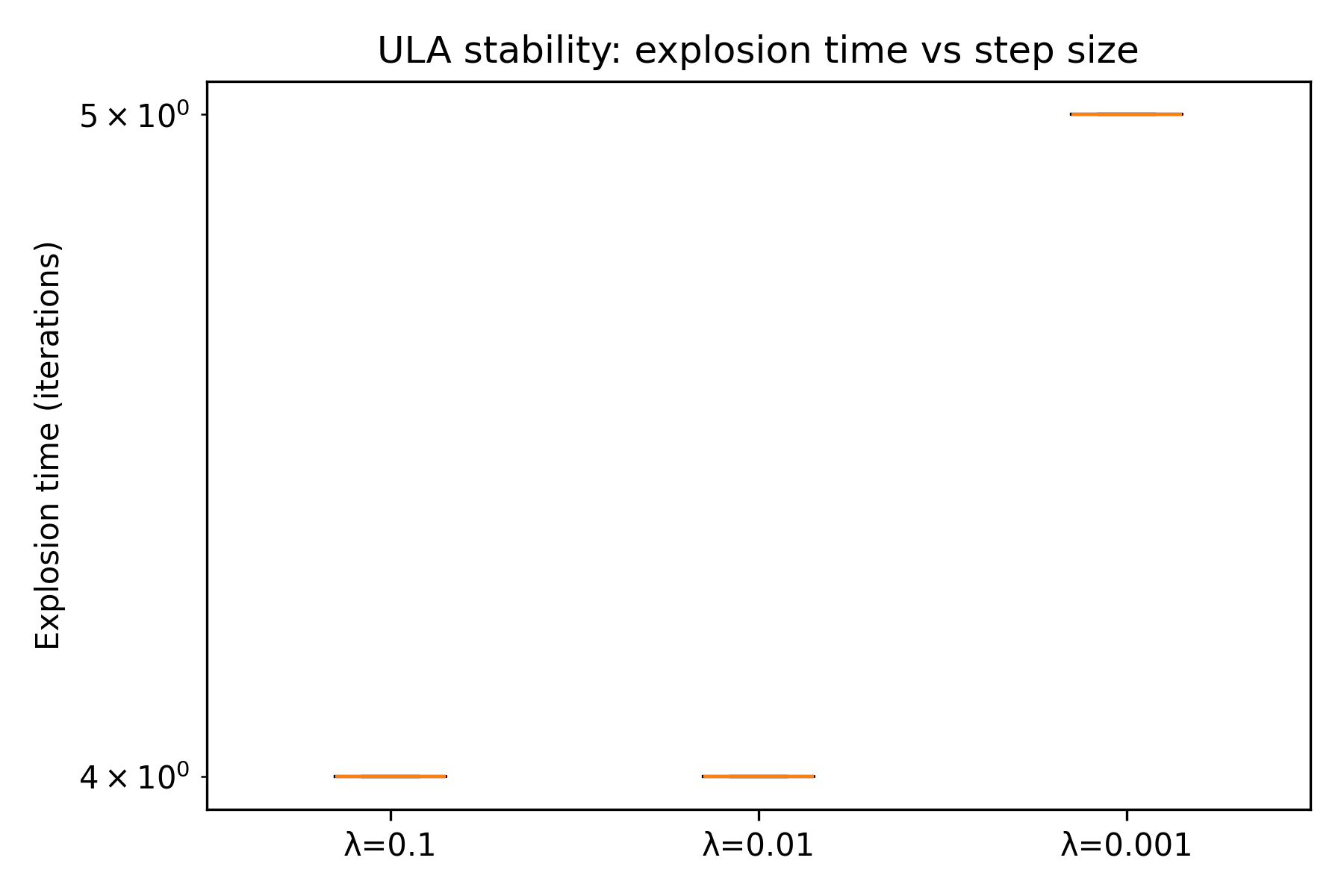
All experiments are performed in dimension $d=100$ with inverse temperature $\beta=1$ . For each stepsize $\lambda\in\{0.1,0.01,0.001\}$ , ULA, kTULA, and tRLMC are run for $N=2\times 10^{5}$ iterations. The initial condition is chosen deterministically as $X_{0}=(200,0,\dots,0)\in\mathbb{R}^{100}$ , placing the system far from equilibrium and in a regime where the superlinear drift dominates. For kTULA and tRLMC, samples are collected after a burn-in period of $5\times 10^{4}$ iterations. Each experiment is repeated independently $30$ times, with all randomness generated from fixed seeds.

To assess stability, we record the explosion time of ULA, defined as the first iteration at which numerical overflow occurs. To assess accuracy for kTULA and tRLMC, we estimate the second moment of the first coordinate and report the absolute error $\bigl|\widehat{\mathbb{E}}[X_{1}^{2}]-\mathbb{E}_{\pi_{\beta}}[X_{1}^{2}]\bigr|$ . Here $\pi_{\beta}$ denotes the invariant law with density proportional to $\exp\!\bigl(-\beta\sum_{i=1}^{d}U(x_{i})\bigr)$ . Since the coordinates are independent under the target distribution, $\mathbb{E}_{\pi_{\beta}}[X_{1}^{2}]$ is the second moment of the associated one-dimensional marginal. In the experiments this reference value is computed numerically by trapezoidal quadrature on a dense grid over $[-4,4]$ .

Refer to caption — (a) ULA explosion time vs. stepsize.

Figure 1 shows a clear separation between the untamed and tamed schemes. For every tested stepsize, ULA becomes unstable after only a few iterations, which is consistent with the known failure of Euler-type Langevin discretizations under superlinear drifts. By contrast, both kTULA and tRLMC remain numerically stable throughout the simulation horizon. Their empirical second-moment error also decreases substantially when the stepsize is reduced from $\lambda=0.1$ to $\lambda=0.01$ , while stability is preserved across all tested values of $\lambda$ .

Table 1. Summary statistics over

30

independent repetitions. For ULA we report explosion time; for kTULA and tRLMC we report the absolute second-moment error. Entries are empirical mean

\pm

standard deviation.

Method	$\lambda=0.1$	$\lambda=0.01$	$\lambda=0.001$
ULA explosion time	$4.00\pm 0.00$	$4.00\pm 0.00$	$5.00\pm 0.00$
kTULA: $\bigl\|\widehat{\mathbb{E}}[X_{1}^{2}]-\mathbb{E}_{\pi_{\beta}}[X_{1}^{2}]\bigr\|$	$0.4336\pm 0.0154$	$0.0453\pm 0.0170$	$0.0455\pm 0.0325$
tRLMC: $\bigl\|\widehat{\mathbb{E}}[X_{1}^{2}]-\mathbb{E}_{\pi_{\beta}}[X_{1}^{2}]\bigr\|$	$0.4025\pm 0.0159$	$0.0428\pm 0.0211$	$0.0437\pm 0.0360$

Table 1 makes the separation quantitative. ULA explodes after roughly four to five iterations for all tested stepsizes. The zero empirical standard deviation for the ULA explosion times indicates that, for each tested stepsize, overflow occurred at the same iteration in all $30$ repetitions from the chosen deterministic initialization. In contrast, both tamed schemes remain stable in all runs.

Figure 2 complements this quantitative comparison by displaying the trajectory behavior of the two tamed schemes at the representative stepsize $\lambda=0.01$ . We plot the evolution of $\|X_{n}\|^{2}$ and the empirical marginal density of the first coordinate against the corresponding one-dimensional marginal of the target law.

The left panel of Figure 2 shows that both tamed schemes enter a stable regime after a short transient and maintain controlled second moments. The center and right panels indicate that the empirical marginals recover the expected bimodal structure of the target distribution, providing further evidence that the tamed schemes remain stable while capturing the qualitative shape of the invariant law.

Taken together, these experiments illustrate the stabilizing effect of taming in the sampling regime. In this aggressive setting, ULA fails almost immediately, whereas kTULA and tRLMC remain stable over long horizons and attain substantially smaller second-moment error once the stepsize is reduced from the coarsest regime.

4.2. Optimization involving a neural network in the fixed-feature setting

We finally consider the optimization problem

\min_{\theta\in\mathbb{R}^{d}}u_{n}(\theta):=\frac{1}{n}\sum_{j=1}^{n}\bigl(Y_{j}-\mathcal{N}(\theta,Z_{j})\bigr)^{2}+\frac{\eta}{6}\sum_{k=1}^{d}|\theta_{k}|^{6},

(13)

where $X_{j}=(Z_{j},Y_{j})\in\mathbb{R}^{m}$ , with $Y_{j}\in\mathbb{R}$ the target variable and $Z_{j}\in\mathbb{R}^{m-1}$ the input variable, $\eta>0$ is a regularization constant, and $\mathcal{N}:\mathbb{R}^{d}\times\mathbb{R}^{m-1}\to\mathbb{R}$ is a single-hidden-layer feed-forward neural network with fixed random features, given by $\mathcal{N}(\theta,z):=\sum_{i=1}^{d_{1}}W_{i}\,\sigma(\langle c_{i},z\rangle+b_{i})$ , where $c_{i}\in\mathbb{R}^{m-1}$ are fixed random feature vectors, $W_{i}\in\mathbb{R}$ are trainable output weights, and $b_{i}\in\mathbb{R}$ are trainable bias parameters. The activation is the sigmoid linear unit $\sigma(x)=x/(1+e^{-x})$ , and the trainable parameter is $\theta=((W_{1},\dots,W_{d_{1}}),(b_{1},\dots,b_{d_{1}}))\in\mathbb{R}^{2d_{1}}$ , so that $d=2d_{1}$ .

We ask whether the provable stability of the tamed schemes manifests in a simple nonlinear problem of the form (13) when the learning rate is taken into an aggressive regime, and whether standard first-order optimizers — which carry no comparable guarantees on (13) — display the deterioration one would expect.

We generate a synthetic regression dataset from a teacher model of the same fixed-feature form. The inputs are sampled from a standard Gaussian distribution in dimension $m-1=20$ ; the teacher network has hidden width $80$ ; independent Gaussian noise with standard deviation $0.05$ is added to the teacher output; and the student network has hidden width $d_{1}=100$ . The training set size is $n=4000$ , the test set size is $1000$ , and training is performed with mini-batches of size $128$ .

We compare SGD, Adam, AMSGrad, kTULA, and tRLMC on the empirical objective (13). For SGD we use momentum $0.9$ . For the two tamed schemes we set $\beta=10^{6}$ , $a=10^{-2}$ , $\ell=4$ , and $\eta=0.05$ . Here $a$ is the linear stabilizing component in the taming map; we fix $a=10^{-2}$ throughout all runs as a small baseline dissipative term. Each method is run for $20$ epochs, repeated over the five seeds $1,2,3,4,5$ , and tested at learning rates $\lambda\in\{0.1,0.2,0.3\}$ .

Figure 3 reports the final test MSE as a function of the learning rate. The main qualitative trend is that the two tamed methods are empirically less sensitive to increasing learning rate than SGD, Adam, and AMSGrad in this synthetic setting. In particular, the three standard optimizers deteriorate substantially as $\lambda$ increases, whereas kTULA varies only moderately across the tested range. tRLMC performs comparably to kTULA at $\lambda=0.1$ and $\lambda=0.2$ , but degrades more noticeably at $\lambda=0.3$ . Since this experiment is small and synthetic, we interpret these results as evidence of a favorable stability trend rather than as a broad benchmark conclusion.

Table 2. Final test MSE over

5

seeds in the fixed-feature neural-network experiment. Entries are empirical mean

\pm

standard deviation across seeds.

Method	$\lambda=0.1$	$\lambda=0.2$	$\lambda=0.3$
SGD	$0.0637\pm 0.0106$	$0.0904\pm 0.0144$	$0.1454\pm 0.0233$
Adam	$0.0978\pm 0.0114$	$0.1363\pm 0.0256$	$0.1509\pm 0.0427$
AMSGrad	$0.0972\pm 0.0112$	$0.1237\pm 0.0214$	$0.1269\pm 0.0285$
kTULA	$0.0542\pm 0.0082$	$0.0589\pm 0.0101$	$0.0630\pm 0.0119$
tRLMC	$0.0520\pm 0.0068$	$0.0565\pm 0.0089$	$0.0716\pm 0.0310$

Table 2 makes the final-error comparison quantitative. In particular, kTULA has the smallest mean final test MSE at $\lambda=0.2$ and $\lambda=0.3$ , while tRLMC is slightly better at $\lambda=0.1$ but becomes more variable at $\lambda=0.3$ .

Figure 4 complements this comparison by displaying the epoch-wise evolution of the parameter norm, test MSE, and training objective at the representative learning rate $\lambda=0.1$ . The parameter-norm panel provides the clearest visual separation between the standard and tamed methods. SGD exhibits steadily increasing norm, while Adam and AMSGrad operate at substantially larger parameter norms throughout training. By contrast, kTULA and tRLMC remain in a much smaller norm regime over the full horizon.

The test-MSE panel suggests that, after the initial transient, the two tamed methods maintain lower average test error than the standard baselines at $\lambda=0.1$ . Likewise, the training-objective panel indicates that kTULA and tRLMC settle at lower objective values, while Adam and AMSGrad level off at visibly higher levels. These plots do not show instability in the strict sense of numerical explosion, but they do indicate that taming leads to more controlled iterates and more stable empirical performance in this regime.

Taken together, these experiments support the same qualitative message as the preceding study. In this nonlinear regression problem with high-order regularization and relatively aggressive learning rates, the tamed Langevin-type schemes display more controlled parameter growth and more robust empirical behavior than SGD, Adam, and AMSGrad. We emphasize, however, that this experiment is intended as a small-scale diagnostic study.

5. Proof outline and technical innovations

The convergence analyses underlying our main results share a common technical core, which we develop in detail in this section. The goal is to bound the divergence between two stochastic processes driven by different Markov kernels: the discrete scheme kTULA or tRLMC on the one hand, and the (SDE) on the other. Classical coupling arguments are tailored to the Wasserstein metric and do not transfer verbatim to information-theoretic divergences such as Kullback–Leibler or total variation. The shifted composition methodology of [5] provides a principled remedy by introducing an auxiliary, third process that interpolates between the two processes of interest. We adapt this methodology to the present setting, where the super-linear growth of the drift induces a state-dependent coupling increment that does not appear in [5]. This is the only point at which the abstract machinery genuinely departs from [5].

Following the two-layer structure of the paper, the local-error frameworks developed in this section—both the KL framework of §5.1–§5.5 and the TV framework of §5.6—are formulated at the level of the (SDE) with general locally Lipschitz drift $h$ , requiring no gradient structure. The Wasserstein convergence argument of §5.7 additionally invokes the sampling specialization $h=\nabla u$ and Assumption (A6), as it relies on the exponential contraction of $(P_{t})_{t\geq 0}$ toward $\pi_{\beta}$ .

5.1. Setup, kernels, and one-step local errors

Fix a step size $\lambda\in(0,1]$ . Let $P=P_{\lambda}$ denote the Markov kernel of (SDE) run for time $\lambda$ , and let $\widehat{P}$ denote the one-step transition kernel of (kTULA). For any $\mu,\nu\in\mathcal{P}_{2}(\mathbb{R}^{d})$ and $n\in\mathbb{N}_{0}$ , set $\widehat{\mu}_{n}:=\mu\,\widehat{P}^{\,n}$ and $\nu_{n}:=\nu\,P^{n}$ . The objective of the framework is to control $\mathrm{KL}(\widehat{\mu}_{N}\,\|\,\nu_{N})$ in terms of one-step, i.e. local, quantities computed at a single iteration.

We work with three measurable functions encoding the one-step discrepancy between $\widehat{P}$ and $P$ :

E_{\mathrm{strong}},E_{\mathrm{weak}}\colon\mathbb{R}^{d}\to[0,\infty),\qquad\Gamma\colon\mathbb{R}^{d}\times\mathbb{R}^{d}\times(0,\infty)\to[0,\infty).

Here $E_{\mathrm{strong}}(x)$ controls the $L^{2}$ -distance between one step of $\widehat{P}$ and one step of $P$ from the same point $x$ ; $E_{\mathrm{weak}}(x)$ is the corresponding bias, which exploits cancellations and is therefore typically smaller than $E_{\mathrm{strong}}(x)$ ; and $\Gamma(x,y,\lambda)$ is a coupling increment controlling the synchronous-coupling distortion between two trajectories of (SDE) started at $x$ and $y$ . For convenience we set

a_{0}(x):=E_{\mathrm{strong}}(x),\qquad a_{1}(x,y):=E_{\mathrm{weak}}(x)+\Gamma(x,y,\lambda)\,E_{\mathrm{strong}}(x).

(14)

The framework is fed by the following one-step Wasserstein bound, verified for kTULA in Lemma 9: there exists $L>0$ such that, for all $x,y\in\mathbb{R}^{d}$ ,

\mathcal{W}_{2}^{2}\!\bigl(\delta_{x}\widehat{P},\delta_{y}P\bigr)\;\leq\;L^{2}\,\|x-y\|^{2}+2\,a_{1}(x,y)\,\|x-y\|+a_{0}(x)^{2}.

(15)

Remark 3 (State-dependence of $a_{1}$ ).

In [5], the coupling increment $\gamma$ is a constant. In the present super-linear setting, the polynomial Lipschitz condition (A2) forces $\Gamma$ to depend on both endpoints, namely $\Gamma(x,y,\lambda)=C_{\mathrm{cpl}}\lambda(1+\|x\|^{\ell^{\prime}}+\|y\|^{\ell^{\prime}})$ . This is the only structural difference between our framework and [5]; as we shall see, it is benign provided uniform moments along the auxiliary process introduced in §5.2 are established.

5.2. The auxiliary interpolating process

The principal obstacle in bounding $\mathrm{KL}(\widehat{\mu}_{N}\,\|\,\nu_{N})$ directly is that $\widehat{\mu}_{N}$ and $\nu_{N}$ are produced by different Markov kernels: any one-step KL bound therefore encodes both the discretization bias and the contraction of the SDE semigroup, and the two effects are difficult to separate. The shifted composition strategy circumvents this obstacle by introducing a third process $(Y_{n}^{\prime})_{n=0}^{N}$ that (i) starts at $\nu_{0}$ , (ii) terminates at $\widehat{\mu}_{N}$ , and (iii) evolves at intermediate steps via the SDE kernel $P$ , so that intermediate one-step KL terms only involve $P$ and are amenable to standard regularity estimates of the semigroup $(P_{t})_{t\geq 0}$ .

Construction.

Let $(\widehat{X}_{n})_{n\geq 0}$ , $(Y_{n})_{n\geq 0}$ denote the kTULA chain and the chain of one-step SDE updates with $\widehat{X}_{0}\sim\mu$ and $Y_{0}\sim\nu$ . Choose shift coefficients $(\eta_{n})_{n=0}^{N-1}\subset[0,1]$ with $\eta_{N-1}=1$ , and define

\widetilde{Y}_{n}:=(1-\eta_{n})\,Y_{n}^{\prime}+\eta_{n}\,\widehat{X}_{n},\qquad n=0,1,\dots,N-1.

(16)

Geometrically, $\widetilde{Y}_{n}$ lies on the segment between $Y_{n}^{\prime}$ and $\widehat{X}_{n}$ ; the parameter $\eta_{n}$ measures how far the auxiliary process is pushed toward the kTULA chain at step $n$ . Define

Q_{n}:=\begin{cases}P,&0\leq n\leq N-2,\\[2.0pt] \widehat{P},&n=N-1,\end{cases}

(17)

and update the auxiliary process by

Y_{n+1}^{\prime}\sim Q_{n}\bigl(\widetilde{Y}_{n},\cdot\bigr),\qquad n=0,1,\dots,N-1,\qquad Y_{0}^{\prime}=Y_{0}.

(18)

We write $\nu_{n}^{\prime}:=\operatorname{Law}(Y_{n}^{\prime})$ .

The terminal condition $\eta_{N-1}=1$ together with the choice $Q_{N-1}=\widehat{P}$ guarantees the interpolation property

\nu_{0}^{\prime}\;=\;\nu_{0},\qquad\nu_{N}^{\prime}\;=\;\widehat{\mu}_{N},

(19)

since $\widetilde{Y}_{N-1}=\widehat{X}_{N-1}$ and the last update applies $\widehat{P}$ to $\widehat{X}_{N-1}$ . Figure 5 illustrates the construction. The freedom to choose $\eta_{n}\in[0,1]$ is what enables the framework to exploit both the contraction of $P$ and the local discretization errors of $\widehat{P}$ : the bounds, determined in Proposition 2, dictate the final iteration complexity.

5.3. KL telescoping via the shifted chain rule

The bridge between the auxiliary process and the KL divergence is the shifted chain rule (3) introduced in Section 2. Recall that the auxiliary variable $X^{\prime}$ allows comparison of Markov updates from different starting points, which is precisely what is needed when the underlying kernels disagree.

We assume the following two one-step KL bounds:

	$\displaystyle\mathrm{KL}\!\bigl(\delta_{x}P\,\\|\,\delta_{y}P\bigr)$	$\displaystyle\;\leq\;c\,\\|x-y\\|^{2},$		(20)
	$\displaystyle\mathrm{KL}\!\bigl(\delta_{x}\widehat{P}\,\\|\,\delta_{y}P\bigr)$	$\displaystyle\;\leq\;c^{\prime}\,\\|x-y\\|^{2}+b(x)^{2},$		(21)

for constants $c,c^{\prime}\geq 0$ and a measurable function $b:\mathbb{R}^{d}\to[0,\infty)$ . We refer to (20) as the regularity of the SDE kernel and to (21) as the cross-regularity of the scheme. For kTULA, both are established in Propositions 5–8.

Lemma 1 (KL telescoping bound).

Let $(Y_{n}^{\prime})_{n=0}^{N}$ and $(\widetilde{Y}_{n})_{n=0}^{N-1}$ be defined by (16)–(18). Then

\mathrm{KL}\!\bigl(\widehat{\mu}_{N}\,\|\,\nu_{N}\bigr)\;\leq\;\sum_{n=0}^{N-1}\mathbb{E}\!\left[\mathrm{KL}\!\bigl(Q_{n}(\widetilde{Y}_{n},\cdot)\,\big\|\,P(Y_{n}^{\prime},\cdot)\bigr)\right].

(22)

If (20)–(21) hold, then

\mathrm{KL}\!\bigl(\widehat{\mu}_{N}\,\|\,\nu_{N}\bigr)\;\leq\;c\,\sum_{n=0}^{N-2}\eta_{n}^{2}\,\mathbb{E}\|\widehat{X}_{n}-Y_{n}^{\prime}\|^{2}+c^{\prime}\,\mathbb{E}\|\widehat{X}_{N-1}-Y_{N-1}^{\prime}\|^{2}+\bar{b}^{\,2},

(23)

where $\bar{b}^{\,2}:=\|b\|_{L^{2}(\widehat{\mu}_{N-1})}^{2}$ .

5.4. Shifted Wasserstein recursion

The right-hand side of (23) is controlled entirely by the squared coupling distances

d_{n}^{\,2}\;:=\;\mathbb{E}\|\widehat{X}_{n}-Y_{n}^{\prime}\|^{2},\qquad n=0,1,\dots,N-1,

(24)

which propagate forward in time according to the next lemma. This is the only place in the analysis where the state-dependent coefficient $a_{1}$ enters.

Lemma 2 (Shifted Wasserstein recursion).

Assume (15). For all $0\leq n\leq N-2$ ,

d_{n+1}^{\,2}\;\leq\;L^{2}(1-\eta_{n})^{2}\,d_{n}^{\,2}+2\,(1-\eta_{n})\,\overline{a}_{1}\,d_{n}+\overline{a}_{0}^{\,2},

(25)

where $\overline{a}_{0}:=\sup_{0\leq k<N}\|a_{0}(\widehat{X}_{k})\|_{L^{2}}$ and $\overline{a}_{1}:=\sup_{0\leq k<N}\|a_{1}(\widehat{X}_{k},\widetilde{Y}_{k})\|_{L^{2}}$ .

Proof.

By the Wasserstein lift of the coupling and (15),

\mathcal{W}_{2}^{2}(\widehat{\mu}_{n+1},\nu_{n+1}^{\prime})\;\leq\;L^{2}\,\mathbb{E}\|\widehat{X}_{n}-\widetilde{Y}_{n}\|^{2}+2\,\mathbb{E}\!\left[a_{1}(\widehat{X}_{n},\widetilde{Y}_{n})\,\|\widehat{X}_{n}-\widetilde{Y}_{n}\|\right]+\mathbb{E}\!\left[a_{0}(\widehat{X}_{n})^{2}\right].

Since $\widehat{X}_{n}-\widetilde{Y}_{n}=(1-\eta_{n})(\widehat{X}_{n}-Y_{n}^{\prime})$ , the first term equals $L^{2}(1-\eta_{n})^{2}d_{n}^{2}$ , Cauchy–Schwarz bounds the cross term by $2(1-\eta_{n})\overline{a}_{1}d_{n}$ , and the third term by $\overline{a}_{0}^{\,2}$ . Choosing the synchronous Wasserstein coupling on the next step yields (25). ∎

Remark 4 (Effect of state-dependence on $\overline{a}_{1}$ ).

The supremum defining $\overline{a}_{1}$ involves the joint law of $(\widehat{X}_{k},\widetilde{Y}_{k})$ , hence requires uniform moment bounds on both $(\widehat{X}_{k})$ and the shifted process $(\widetilde{Y}_{k})$ . Since $\widetilde{Y}_{k}$ is a convex combination of $Y_{k}^{\prime}$ and $\widehat{X}_{k}$ , controlling its moments reduces to controlling those of $Y_{k}^{\prime}$ , which we establish in Lemma 10 via the dissipativity condition (A4) on the drift of (SDE). This is the only place where the polynomial-Lipschitz nature of the drift plays a non-trivial role at the level of the framework.

The recursion (25) is purely deterministic once $\overline{a}_{0},\overline{a}_{1},L$ have been fixed. Its analysis is identical to that of the corresponding recursion in [5, Lemma B.5], and yields the following optimal control of the shifted distances.

Proposition 2 (Deterministic control of the shifted distances).

Let $L\in[\tfrac{1}{2},2]$ , $\overline{a}_{0},\overline{a}_{1}\geq 0$ , and $\bar{N}:=N\wedge 1/(1-L)_{+}$ . There exists a sequence $(\eta_{n})_{n=0}^{N-2}\subset[0,1]$ with $\eta_{N-1}=1$ such that any nonnegative sequence $(d_{n})_{n=0}^{N-1}$ satisfying (25) and $d_{0}=\mathcal{W}_{2}(\mu,\nu)$ obeys

	$\displaystyle d_{N-1}^{\,2}$	$\displaystyle\;\lesssim\;\tfrac{L^{-1}-1}{L^{-N}-1}\,d_{0}^{\,2}+\bigl(((L-1)N)\vee\log\bar{N}\bigr)\,\overline{a}_{0}^{\,2}+\bar{N}\,\overline{a}_{1}^{\,2},$		(26)
	$\displaystyle\sum_{n=0}^{N-2}\eta_{n}^{2}\,d_{n}^{\,2}$	$\displaystyle\;\lesssim\;\tfrac{L^{-1}-1}{L^{-N}-1}\,d_{0}^{\,2}+\bigl(((L-1)N)\vee\log\bar{N}\bigr)\,\overline{a}_{0}^{\,2}+\bar{N}\,\overline{a}_{1}^{\,2}.$		(27)

Proof.

The recursion (25) has the same form as the recursion analyzed in [5, Appendix B.2], with deterministic coefficients $\overline{a}_{0},\overline{a}_{1}$ in place of the local errors used there. The optimal shift sequence and the dynamic programming argument of [5, Lemmas B.4–B.6] apply verbatim and yield (26)–(27). ∎

5.5. The KL local-error bound for kTULA

Combining Lemma 1 with Proposition 2 yields the main KL bound of the framework.

Theorem 4 (KL local-error framework).

Assume (15), (20), and (21), and let $L\in[\tfrac{1}{2},2]$ . With $\overline{a}_{0},\overline{a}_{1}$ as in Lemma 2, $\bar{b}:=\max_{0\leq n<N}\|b\|_{L^{2}(\widehat{\mu}_{n})}$ , and $\bar{N}=N\wedge 1/(1-L)_{+}$ ,

\mathrm{KL}\!\bigl(\mu\widehat{P}^{N}\,\|\,\nu P^{N}\bigr)\;\lesssim\;(c+c^{\prime})\!\left[\tfrac{L^{-1}-1}{L^{-N}-1}\,\mathcal{W}_{2}^{2}(\mu,\nu)+\bigl(((L-1)N)\vee\log\bar{N}\bigr)\,\overline{a}_{0}^{\,2}+\bar{N}\,\overline{a}_{1}^{\,2}\right]+\bar{b}^{\,2}.

(28)

We emphasize that the bound (28) compares the discretization $\mu\widehat{P}^{N}$ against the law $\nu P^{N}$ of the (SDE); no invariant-measure or gradient structure is invoked at this stage. The specialization to sampling toward $\pi_{\beta}$ proceeds via the additional ergodicity input provided by Assumption (A6), as carried out in Section 3.

5.6. A TV bound for the randomized scheme tRLMC

For the tamed randomized midpoint scheme tRLMC, the KL framework above is not directly applicable: the randomization of the integration time prevents the natural construction of an adapted continuous-time interpolation, and consequently a sharp cross-regularity estimate of the form (21) is not currently available. We therefore work in the weaker total variation metric, where a direct one-step estimate is at hand.

Let $\widetilde{P}$ denote the one-step kernel of tRLMC, and write $\widetilde{\mu}_{n}:=\mu\widetilde{P}^{\,n}$ . We assume, in addition to the regularity (20), the existence of a one-step TV local error: there exists a measurable function $C_{\mathrm{TV}}\colon\mathbb{R}^{d}\to[0,\infty)$ such that, for all $x\in\mathbb{R}^{d}$ ,

TV\!\bigl(\delta_{x}\widetilde{P},\delta_{x}P\bigr)\;\leq\;C_{\mathrm{TV}}(x)\,\lambda.

(29)

For tRLMC, this estimate is established in Proposition 11.

The auxiliary process construction of §5.2 remains valid with $\widehat{P}$ replaced by $\widetilde{P}$ throughout.

Lemma 3 (TV bound via the shifted construction).

Assume (20) and (29), and let $d_{n}^{\,2}:=\mathbb{E}\|\widetilde{X}_{n}-Y_{n}^{\prime}\|^{2}$ . Writing $\overline{C}_{\mathrm{TV}}:=\sup_{0\leq n<N}\|C_{\mathrm{TV}}(x)\|_{L^{2}(\widetilde{\mu}_{n})}$ ,

TV\!\bigl(\widetilde{\mu}_{N},\nu_{N}\bigr)\;\leq\;\overline{C}_{\mathrm{TV}}\,\lambda+\sqrt{\tfrac{c}{2}}\,d_{N-1}+\sqrt{\tfrac{c}{2}\,\sum_{n=0}^{N-2}\eta_{n}^{2}\,d_{n}^{\,2}}.

(30)

Theorem 5 (TV local-error framework).

Assume (15), (20), and (29), and let $L\in[\tfrac{1}{2},2]$ . With $\overline{a}_{0},\overline{a}_{1}$ as in Lemma 2 (with $\widehat{P}$ replaced by $\widetilde{P}$ ) and $\bar{N}=N\wedge 1/(1-L)_{+}$ ,

TV\!\bigl(\mu\widetilde{P}^{N},\nu P^{N}\bigr)\;\lesssim\;\overline{C}_{\mathrm{TV}}\,\lambda+\sqrt{\tfrac{L^{-1}-1}{L^{-N}-1}\,\mathcal{W}_{2}^{2}(\mu,\nu)+\bigl(((L-1)N)\vee\log\bar{N}\bigr)\,\overline{a}_{0}^{\,2}+\bar{N}\,\overline{a}_{1}^{\,2}}.

(31)

The proof combines Lemma 3 with Proposition 2. The KL and TV frameworks rest on the same shifted Wasserstein recursion and differ only at the terminal step: the KL framework requires the cross-regularity estimate (21), whereas the TV framework only requires (29), making Theorem 5 applicable to schemes such as tRLMC for which a sharp cross-regularity estimate is currently out of reach. As with Theorem 4, the bound (31) is stated against the law $\nu P^{N}$ of (SDE) and requires no gradient structure on the drift.

5.7. Wasserstein convergence of tRLMC

Wasserstein convergence for tRLMC avoids the auxiliary process construction and proceeds via a more direct route based on the contraction of the underlying semigroup toward $\pi_{\beta}$ . Unlike the local-error frameworks of §5.1–§5.6, this argument is genuinely sampling-specific: throughout the present subsection we therefore assume the specialization $h=\nabla u$ , $\sigma=\sqrt{2/\beta}$ of (SDE) to the (LSDE), and we additionally impose Assumption (A6).

Under this specialization, the local Lipschitz property of the drift, combined with the one-sided Lipschitz condition (A3), yields a one-step Wasserstein bound of the form (15) with $\Gamma(x,y,\lambda)=C_{\mathrm{cpl}}\lambda(1+\|x\|^{2\ell}+\|y\|^{2\ell})$ . Iterating this estimate over $n_{0}$ steps and exploiting the uniform moment bounds of Lemma 12 furnishes the long-time discretization-error estimate

\mathcal{W}_{2}\!\left(\mu_{0}\widetilde{P}^{\,n},\;\bigl(\mu_{0}\widetilde{P}^{\,n-n_{0}}\bigr)P^{n_{0}}\right)\;\leq\;C\,e^{c\lambda n_{0}}\,\lambda,\qquad n\geq n_{0}\geq 0,

(32)

where $C,c$ depend polynomially on the dimension. In parallel, the combination of the logarithmic Sobolev inequality (A6) and the one-sided Lipschitz condition (A3) implies the contraction

\mathcal{W}_{2}\!\bigl(\nu P^{t},\pi_{\beta}\bigr)\;\leq\;C_{\mathrm{contr}}\,e^{-\dot{c}\,t}\,\mathcal{W}_{2}\!\bigl(\nu,\pi_{\beta}\bigr),\qquad t\geq 0,

(33)

for some $\dot{c}>0$ depending on $C_{\mathrm{LSI}}$ . Combining (32) and (33) via the triangle inequality

\mathcal{W}_{2}\!\bigl(\mu_{0}\widetilde{P}^{\,n},\pi_{\beta}\bigr)\;\leq\;\mathcal{W}_{2}\!\Bigl(\mu_{0}\widetilde{P}^{\,n},\,\bigl(\mu_{0}\widetilde{P}^{\,n-n_{0}}\bigr)P^{n_{0}}\Bigr)+\mathcal{W}_{2}\!\Bigl(\bigl(\mu_{0}\widetilde{P}^{\,n-n_{0}}\bigr)P^{n_{0}},\pi_{\beta}\Bigr),

and balancing the two contributions by an appropriate choice of $n_{0}$ yields the announced Wasserstein convergence estimate of Theorem 3.

Appendix A Drift Properties and Moment Estimates

This appendix collects technical estimates underlying the analysis. We record structural properties of the tamed drift, including dissipativity, growth, and global Lipschitz bounds, and establish uniform moment bounds for both the underlying LSDE and the kTULA iterates. We also include a local Taylor remainder estimate under polynomially growing Jacobian regularity, which is used in the control of one-step discretization errors. Proofs are deferred to Section D unless otherwise stated.

A.1. Properties of the tamed drift

Lemma 4 (Key properties of the tamed drift).

Assume that (A1), (A2), and (A4) hold. Then for any $\theta,\bar{\theta}\in\mathbb{R}^{d}$ and any $0<\lambda<1$ , the following statements hold.

(i)

Dissipativity. The tamed drift satisfies

$\langle h_{\lambda}(\theta),\theta\rangle\geq a\|\theta\|^{2}-b.$

(ii)

Growth control. The magnitude of $h_{\lambda}$ satisfies

\|h_{\lambda}(\theta)\|\leq 2a\|\theta\|+2L\,\lambda^{-1/2},\qquad\|h_{\lambda}(\theta)\|\leq(2a+L)\bigl(1+\|\theta\|^{\ell+1}\bigr).

(iii)

Lipschitz continuity. There exists a constant $L_{0}>0$ , depending only on $a,L,\ell$ , such that

$\|h_{\lambda}(\theta)-h_{\lambda}(\bar{\theta})\|\leq L_{0}\,\lambda^{-1/2}\,\|\theta-\bar{\theta}\|,$

where

$L_{0}:=2a+4L+(\ell+1)(2L+a).$
(iv)

Taming error. The deviation between the original and tamed drifts satisfies

$\|h(\theta)-h_{\lambda}(\theta)\|^{2}\leq 4\lambda^{2}(L+a)^{2}\bigl(1+\|\theta\|^{\,6(\ell+1)}\bigr).$

Proof.

The result follows from [22, Lemma 4.1] specialized to $\varepsilon_{h}=\frac{1}{2}$ . ∎

A.2. Moment bounds for the underlying SDE

Lemma 5 (Uniform $2p$ -moment bounds for LSDE).

Let Assumptions (A1)–(A4) hold, and let $(X_{t})_{t\geq 0}$ solve LSDE with $X_{0}=x$ . Then for any $p\in\mathbb{N}$ there exist constants $c_{p}>0$ and $C_{p}>0$ such that for all $t\geq 0$ ,

\mathbb{E}\|X_{t}\|^{2p}\;\leq\;e^{-c_{p}t}\,\|x\|^{2p}\;+\;C_{p},

where one can take

c_{p}=pa,\qquad C_{p}=C\Bigl(b+\tfrac{1}{\beta}(d+2(p-1))\Bigr)^{p}

for a constant $C>0$ depending only on $p$ .

Proof.

The proof follows from [18, Lemma A.1]. ∎

Lemma 6 (One-step $p$ -moment drift for LSDE).

Fix $p\geq 2$ . Under Assumption (A4), there exist constants $q>0$ and $C_{p}>0$ , depending only on $p$ , $d$ , $a$ , $b$ , and $\beta$ , such that for every $\lambda\in(0,1]$ and every $x\in\mathbb{R}^{d}$ ,

\mathbb{E}\|X(t,x;t+\lambda)\|^{p}\leq e^{-q\lambda}\|x\|^{p}+C_{p}\lambda,

where $X(t,x;\cdot)$ denotes the solution of (LSDE) started from $x$ at time $t$ .

Proof.

The proof is given in D.1.1. ∎

A.3. Moment bounds for the kTULA scheme

We now establish uniform-in-time moment bounds for the kTULA chain.

Lemma 7 (Uniform moments for the (kTULA) scheme).

Let Assumptions (A1)–(A4) hold. There exists $\lambda_{\max}>0$ such that for all $0<\lambda\leq\lambda_{\max}$ the following holds. Let $(\widehat{X}_{n})_{n\geq 0}$ denote the kTULA iterates and let $\widehat{X}_{t}$ be any continuous interpolation on $[n\lambda,(n+1)\lambda]$ satisfying $\widehat{X}_{n\lambda}=\widehat{X}_{n}$ . Then for every $p\geq 2$ there exists a constant $c_{p}<\infty$ such that for all $t\in[n\lambda,(n+1)\lambda]$ ,

\mathbb{E}\|\widehat{X}_{t}\|^{2p}\;\leq\;(1-a(t-n\lambda))(1-a\lambda)^{n}\,\mathbb{E}\|\widehat{X}_{0}\|^{2p}+c_{p}\Bigl(1+\frac{1}{a}\Bigr).

In particular,

\sup_{t\geq 0}\mathbb{E}\|\widehat{X}_{t}\|^{2p}\;\leq\;\mathbb{E}\|\widehat{X}_{0}\|^{2p}+c_{p}\Bigl(1+\frac{1}{a}\Bigr)<\infty.

Proof.

The result follows from [22, Lemma 4.2]. ∎

A.4. A local smoothness remainder bound

We close this appendix with an elementary Taylor remainder estimate that will be invoked repeatedly when controlling one-step discretization errors under polynomially growing local smoothness of the Jacobian.

Lemma 8 (Taylor remainder under locally Lipschitz Jacobian).

Let $h:\mathbb{R}^{d}\to\mathbb{R}^{d}$ be continuously differentiable. Under Assumption (A5), for all $x,y\in\mathbb{R}^{d}$ ,

\big\|h(x)-h(y)-J(h)(x)(x-y)\big\|\leq\frac{L^{\prime\prime}}{2}\,(1+\|x\|+\|y\|)^{\ell^{\prime\prime}}\,\|x-y\|^{2}.

Proof.

A Taylor expansion of $h\bigl(y+t(x-y)\bigr)$ for $t\in[0,1]$ , combined with (A5) to bound the increment of the Jacobian $J(h)$ , yields the claim. ∎

Appendix B Local Error Tools and Regularity

This appendix collects auxiliary estimates for the underlying (SDE) that are used to verify the local-error framework. In particular, we establish $W_{2}$ -Lipschitz continuity, derive a coupling increment bound, and record the resulting one-step Wasserstein estimate together with a KL regularity bound.

Proposition 3 ( $W_{2}$ –Lipschitz continuity).

Assume (A3). Let $(X_{t})_{t\geq 0}$ and $(Y_{t})_{t\geq 0}$ be solutions of (SDE) driven by the same Brownian motion, with initial conditions $X_{0}=x$ and $Y_{0}=y$ . Then for all $t\geq 0$ ,

\|X_{t}-Y_{t}\|_{L^{2}}\leq e^{K^{\prime}t}\,\|x-y\|.

In particular, for $t\in[0,\lambda]$ , setting $L:=e^{K^{\prime}\lambda}$ yields

\|X_{t}-Y_{t}\|_{L^{2}}\leq L\,\|x-y\|.

For $\lambda\leq\frac{\ln 2}{|K^{\prime}|}$ , then $L\in[\tfrac{1}{2},2]$ .

Proof.

The proof is given in Subsection D.2.1. ∎

Proposition 4 (Coupling increment).

Assume (A1)–(A3). There exists a constant $C_{\mathrm{cpl}}>0$ , depending on $L^{\prime}$ , $\ell^{\prime}$ , and $\beta$ , such that for all $t\in[0,\lambda]$ , with $\lambda\leq\frac{\ln 2}{|K^{\prime}|}$ ,

\|X_{t}-x-(Y_{t}-y)\|_{L^{2}}\;\leq\;\Gamma(x,y,t)\,\|x-y\|,

where $(X_{t})_{t\geq 0}$ , $(Y_{t})_{t\geq 0}$ are solutions of (LSDE) driven by the same Brownian motion with $X_{0}=x$ , $Y_{0}=y$ , and

\Gamma(x,y,t):=C_{\mathrm{cpl}}\,t\,\bigl(1+\|x\|^{\ell^{\prime}}+\|y\|^{\ell^{\prime}}\bigr).

In particular, taking $t=\lambda$ yields

\Gamma(x,y,\lambda):=C_{\mathrm{cpl}}\,\lambda\,\bigl(1+\|x\|^{\ell^{\prime}}+\|y\|^{\ell^{\prime}}\bigr).

Proof.

The proof is given in Subsection D.2.2. ∎

Lemma 9 (One-step Wasserstein inequality).

Let $L>0$ be the $W_{2}$ -Lipschitz constant from Proposition 3, let $\Gamma(x,y,\lambda)$ be the coupling increment from Proposition 4, and let $E_{\mathrm{weak}},E_{\mathrm{strong}}:\mathbb{R}^{d}\to[0,\infty)$ denote the weak and strong one-step local errors of (kTULA) (Propositions 6–7). Then, for all $x,y\in\mathbb{R}^{d}$ ,

\mathcal{W}_{2}^{2}(\delta_{x}\widehat{P},\delta_{y}P)\leq L^{2}\|x-y\|^{2}+2\Bigl(E_{\mathrm{weak}}(x)+\Gamma(x,y,\lambda)\,E_{\mathrm{strong}}(x)\Bigr)\|x-y\|+E_{\mathrm{strong}}(x)^{2}.

Proof.

The result follows by the same argument as in [5], with the only difference that here the coupling increment $\Gamma(x,y,\lambda)$ depends on both endpoints rather than only on $x$ , leading to the state-dependent coefficient. ∎

Remark 5.

With the notation

a_{0}(x):=E_{\mathrm{strong}}(x),\qquad a_{1}(x,y):=E_{\mathrm{weak}}(x)+\Gamma(x,y,\lambda)E_{\mathrm{strong}}(x),

the one-step Wasserstein estimate takes the form

\mathcal{W}_{2}^{2}(\delta_{x}\widehat{P},\delta_{y}P)\leq L^{2}\|x-y\|^{2}+2a_{1}(x,y)\|x-y\|+a_{0}(x)^{2}.

Proposition 5 (Regularity [32, Theorem 1.1]).

Let $P=P_{\lambda}$ denote the one-step kernel of (SDE). There exists a constant $C_{\mathrm{reg}}>0$ , depending on $\beta$ , such that for all $x,y\in\mathbb{R}^{d}$ and all $t\in(0,\lambda]$ ,

\mathrm{KL}\!\bigl(\delta_{x}P_{t}\,\big\|\,\delta_{y}P_{t}\bigr)\;\leq\;R_{2}(\delta_{x}P_{t},\delta_{y}P_{t})\;\leq\;\frac{C_{\mathrm{reg}}}{1-e^{-K^{\prime}t}}\,\|x-y\|^{2}.

In particular, if $K^{\prime}\lambda\leq 2$ , then at $t=\lambda$ one may take

c=\frac{3C_{\mathrm{reg}}}{\lambda}.

Appendix C Auxiliary Results for the Main Theorems

This appendix collects auxiliary results used in the proofs of the main convergence theorems. We record the strong and weak local error bounds, cross-regularity estimates, and shifted moment controls needed for kTULA, together with the corresponding moment, local-error, total variation, and Wasserstein tools for the tamed randomized scheme.

C.1. Strong and weak local errors of kTULA

Proposition 6 (Weak local error).

Let Assumptions (A1)–(A5) hold. Let $X_{t}$ denote the solution of (LSDE) started from $X_{0}=x$ , and $\widehat{X}_{t}$ the one-step interpolation associated with (kTULA) started from $\widehat{X}_{0}=x$ . Set $M:=\max\{3(\ell+1),\,4\ell+\ell^{\prime\prime}\}$ . Then there exists a constant $C>0$ , independent of $x\in\mathbb{R}^{d}$ , $d$ , and $\lambda\in(0,1]$ , such that for every $x\in\mathbb{R}^{d}$ ,

\big\|\mathbb{E}[\widehat{X}_{\lambda}]-\mathbb{E}[X_{\lambda}]\big\|\;\leq\;C\bigl(1+d^{M/2}+\|x\|^{M}\bigr)\,\lambda^{2}.

In particular,

E_{\mathrm{weak}}(x):=C\bigl(1+d^{M/2}+\|x\|^{M}\bigr)\,\lambda^{2}.

Proof.

The proof is given in Subsection D.3.1. ∎

Proposition 7 (Strong local error).

Let Assumptions (A1)–(A4) hold. Let $X_{t}$ denote the solution of (LSDE) started from $X_{0}=x$ , and $\widehat{X}_{t}$ the one-step interpolation associated with (kTULA) started from $\widehat{X}_{0}=x$ . Set $M:=\max\{3(\ell+1),\,2\ell^{\prime}+4\ell\}$ . Then there exists a constant $C>0$ , independent of $x\in\mathbb{R}^{d}$ , $d$ , and $\lambda\in(0,1]$ , such that for every $x\in\mathbb{R}^{d}$ ,

\|\widehat{X}_{\lambda}-X_{\lambda}\|_{L^{2}}\;\leq\;C\bigl(1+d^{M/2}+\|x\|^{M}\bigr)\,\lambda^{3/2}.

In particular,

E_{\mathrm{strong}}(x):=C\bigl(1+d^{M/2}+\|x\|^{M}\bigr)\,\lambda^{3/2}.

Proof.

The proof is given in Subsection D.3.2. ∎

C.2. Cross-regularity for kTULA

Proposition 8 (Cross-regularity).

Assume (A1)–(A4). There exist a constant $C_{\mathrm{cross}}>0$ and a measurable function $b:\mathbb{R}^{d}\to[0,\infty)$ such that, for all $x,y\in\mathbb{R}^{d}$ and all $t\in(0,\lambda]$ ,

\mathrm{KL}\!\bigl(\delta_{x}\widehat{P}\,\big\|\,\delta_{y}P_{t}\bigr)\;\leq\;\frac{C_{\mathrm{cross}}}{1-e^{-K^{\prime}t}}\,\|x-y\|^{2}\;+\;b(x)^{2},

where

b(x)^{2}\leq C\,\lambda^{2}\bigl(1+\|x\|^{2\ell+2}\bigr).

In particular, taking $t=\lambda$ , one may take

c^{\prime}=\frac{C_{\mathrm{cross}}}{\lambda}.

Proof.

The proof is given in Subsection D.3.3. ∎

C.3. Shifted recursion and auxiliary moment control for kTULA

Lemma 10 (Uniform moment bounds for the shifted process).

Let $p\geq 1$ and define the shifted process $\widetilde{Y}_{n}:=(1-\eta_{n})Y_{n}^{\prime}+\eta_{n}\widehat{X}_{n}$ for $n\geq 0$ . Under the hypotheses of Lemma 6 (with constants $q,C>0$ ), and assuming $\widehat{M}_{p}:=\sup_{n\geq 0}\mathbb{E}\|\widehat{X}_{n}\|^{p}<\infty$ , we have

\mathbb{E}\|\widetilde{Y}_{n}\|^{p}\leq e^{-q\lambda n}\mathbb{E}\|\widetilde{Y}_{0}\|^{p}+\frac{C\lambda+\widehat{M}_{p}}{1-e^{-q\lambda}},

yielding the uniform bound $\sup_{n\geq 0}\mathbb{E}\|\widetilde{Y}_{n}\|^{p}\leq\mathbb{E}\|\widetilde{Y}_{0}\|^{p}+\frac{C\lambda+\widehat{M}_{p}}{1-e^{-q\lambda}}<\infty$ .

Proof.

The proof is given in Subsection D.3.4. ∎

Lemma 11 (Shifted distance recursion).

Let $E_{\mathrm{weak}}$ , $E_{\mathrm{strong}}$ , and $\Gamma$ denote the weak-error, strong-error, and coupling-increment functions of Propositions 6, 7, and 4, and set

a_{0}(x):=E_{\mathrm{strong}}(x),\qquad a_{1}(x,y):=E_{\mathrm{weak}}(x)+\Gamma(x,y,\lambda)\,E_{\mathrm{strong}}(x).

For $0\leq n\leq N-1$ , let $\eta_{n}\in[0,1]$ , $\widetilde{Y}_{n}:=(1-\eta_{n})Y_{n}^{\prime}+\eta_{n}\widehat{X}_{n}$ , and $d_{n}^{2}:=\mathbb{E}\|\widehat{X}_{n}-Y_{n}^{\prime}\|^{2}$ , and put

\overline{a}_{0}:=\sup_{0\leq k<N}\|a_{0}(\widehat{X}_{k})\|_{L^{2}},\qquad\overline{a}_{1}:=\sup_{0\leq k<N}\|a_{1}(\widehat{X}_{k},\widetilde{Y}_{k})\|_{L^{2}}.

Then, with $L:=e^{K^{\prime}\lambda}$ , for every $0\leq n\leq N-2$ ,

d_{n+1}^{2}\leq L^{2}(1-\eta_{n})^{2}\,d_{n}^{2}+2(1-\eta_{n})\,\overline{a}_{1}\,d_{n}+\overline{a}_{0}^{\,2}.

Proof.

The proof is given in Subsection D.3.5. ∎

C.4. Auxiliary moment bounds for tRLMC

Lemma 12 (Uniform moments for tRLMC).

Assume (A1), (A2), and (A4). Let $(\bar{Y}_{n})_{n\geq 0}$ denote the tamed randomized Langevin Monte Carlo scheme (tRLMC), initialized at $\bar{Y}_{0}=x_{0}\in\mathbb{R}^{d}$ . Then the following statements hold.

(i)

There exist constants $\lambda_{2,\max}^{tRLMC}>0$ , $\mu>0$ , and $M_{2}>0$ , depending only on $a,b,L,L_{0},\beta$ , such that for every $\lambda\in(0,\lambda_{2,\max}^{tRLMC}]$ ,

$\mathbb{E}\|\bar{Y}_{n}\|^{2}\leq e^{-\mu n\lambda}\,\mathbb{E}\|x_{0}\|^{2}+M_{2}\,d,\qquad n\in\mathbb{N}_{0}.$

(ii)

For every $p\in[2,4\ell]\cap\mathbb{N}$ , there exist constants $\lambda_{p,\max}^{tRLMC}>0$ , $c_{p}>0$ , and $\widetilde{C}_{p}>0$ , depending only on $p,a,b,L,L_{0},\beta$ , such that for every $\lambda\in(0,\lambda_{p,\max}^{tRLMC}]$ ,

\mathbb{E}\|\bar{Y}_{n}\|^{2p}\leq(1-c_{p}\lambda)^{n}\,\mathbb{E}\|x_{0}\|^{2p}+\widetilde{C}_{p}(1+d^{p}),\qquad n\in\mathbb{N}_{0}.

In particular,

\sup_{n\geq 0}\mathbb{E}\|\bar{Y}_{n}\|^{2p}<\infty.

Proof.

The proof of (i) is given in Subsection D.4.1, and the proof of (ii) is given in Subsection D.4.2. ∎

Lemma 13 (One-step $p$ -moment drift for RLMC).

Fix $p\geq 2$ . Under Assumption (A4), there exist constants $q>0$ and $C_{p}>0$ , depending only on $p$ , $d$ , $a$ , $b$ , and $\beta$ , such that for all $\lambda\in(0,1]$ ,

\mathbb{E}\|Y^{\prime}_{n+1}\|^{p}\leq e^{-q\lambda}\,\mathbb{E}\|\widetilde{Y}_{n}\|^{p}+C_{p}\lambda,

where

Y^{\prime}_{n+1}\sim P_{\lambda}(\widetilde{Y}_{n},\cdot),\qquad\widetilde{Y}_{n}=(1-\eta_{n})Y_{n}^{\prime}+\eta_{n}\bar{Y}_{n},\qquad\eta_{n}\in[0,1].

Proof.

The proof is given in Subsection D.4.3. ∎

Lemma 14 (Uniform moment bounds for the shifted process under tRLMC).

Let $p\geq 2$ and define the shifted process $\widetilde{Y}_{n}:=(1-\eta_{n})Y_{n}^{\prime}+\eta_{n}\bar{Y}_{n}$ for $n\geq 0$ . Under the hypotheses of Lemma 13 (with constants $q,C_{p}>0$ ), and assuming $\bar{M}_{p}:=\sup_{n\geq 0}\mathbb{E}\|\bar{Y}_{n}\|^{p}<\infty$ , we have

\mathbb{E}\|\widetilde{Y}_{n}\|^{p}\leq e^{-q\lambda n}\mathbb{E}\|\widetilde{Y}_{0}\|^{p}+\frac{C_{p}\lambda+\bar{M}_{p}}{1-e^{-q\lambda}},

yielding the uniform bound $\sup_{n\geq 0}\mathbb{E}\|\widetilde{Y}_{n}\|^{p}\leq\mathbb{E}\|\widetilde{Y}_{0}\|^{p}+\frac{C_{p}\lambda+\bar{M}_{p}}{1-e^{-q\lambda}}<\infty$ .

Proof.

The proof is given in Subsection D.4.4. ∎

C.5. Weak and strong local errors for tRLMC

Proposition 9 (Weak error for tRLMC).

Assume (A1), (A2), and (A4). Let $X(t,x;t+\lambda)$ denote the solution of (LSDE) at time $t+\lambda$ , starting from $X_{t}=x$ , and let $\lambda\in(0,1)$ . Let $\bar{Y}(t,x;t+\lambda)$ be the one-step tamed randomized midpoint approximation defined in (tRLMC). Set $R:=3(\ell+1)$ . Then, for all $t\geq 0$ and $x\in\mathbb{R}^{d}$ , there exists a constant $C>0$ , independent of $d,t,x,\lambda$ , such that

\bigl\|\mathbb{E}\!\bigl[X(t,x;t+\lambda)-\bar{Y}(t,x;t+\lambda)\bigr]\bigr\|\;\leq\;C\,\bigl(1+d^{R/2}+\|x\|^{R}\bigr)\lambda^{2}.

Proof.

The proof is given in Subsection D.4.5. ∎

Proposition 10 (Strong error for tRLMC).

Assume (A1), (A2), and (A4). Let $X(t,x;t+\lambda)$ denote the solution of (SDE) at time $t+\lambda$ , starting from $X_{t}=x$ , and let $\lambda\in(0,1)$ . Let $\bar{Y}(t,x;t+\lambda)$ be the one-step tamed randomized midpoint approximation defined in (tRLMC). Set $\widetilde{R}:=\max\{2\ell^{\prime}+4\ell,\,6(\ell+1)\}$ . Then, for all $t\geq 0$ and $x\in\mathbb{R}^{d}$ , there exists a constant $C>0$ , independent of $d,t,x,\lambda$ , such that

\mathbb{E}\bigl[\|X(t,x;t+\lambda)-\bar{Y}(t,x;t+\lambda)\|^{2}\bigr]\;\leq\;C\,\bigl(1+d^{\widetilde{R}}+\|x\|^{2\widetilde{R}}\bigr)\lambda^{3}.

Proof.

The proof is given in Subsection D.4.6. ∎

C.6. Total variation estimates for tRLMC

Proposition 11 (Cross-TV regularity for tRLMC).

There exist a constant $C>0$ and a measurable function $C_{\mathrm{TV}}:\mathbb{R}^{d}\to[0,\infty)$ such that, for all $x,y\in\mathbb{R}^{d}$ ,

\mathrm{TV}(\delta_{x}\widetilde{P},\delta_{y}P)\;\leq\;C_{\mathrm{TV}}(x)\,\lambda\;+\;C\,\frac{\|x-y\|}{\sqrt{\lambda}}.

Proof.

The proof is given in Section D.4.7. ∎

Lemma 15 (TV bound via the shifted construction).

Assume (20) and (29). Let

d_{n}^{2}:=\mathbb{E}\|\bar{Y}_{n}-Y_{n}^{\prime}\|^{2}.

Then

\mathrm{TV}(\widetilde{\mu}_{N},\nu_{N})\leq\overline{C}_{\mathrm{TV}}\,\lambda+\sqrt{\tfrac{c}{2}}\,d_{N-1}+\sqrt{\tfrac{c}{2}\sum_{n=0}^{N-2}\eta_{n}^{2}\,d_{n}^{2}},

(34)

where $c=\mathcal{O}(\lambda^{-1})$ .

Proof.

The proof is given in Section D.4.8. ∎

C.7. Wasserstein convergence for tRLMC

Throughout this subsection, we work in the sampling specialization $h=\nabla u$ , $\sigma=\sqrt{\frac{2}{\beta}}$ , under Assumption (A6). We denote by $P$ the one-step Langevin kernel of (LSDE), and by $\widetilde{P}$ the one-step kernel of (tRLMC).

Lemma 16.

For any $n,n_{0}\in\mathbb{N}$ ,

W_{2}\!\bigl(\mu_{0}\widetilde{P}^{n},\,\bigl(\mu_{0}\widetilde{P}^{\,n-n_{0}}\bigr)P^{n_{0}}\bigr)\;\leq\;C_{d}\,e^{\frac{3}{2}K^{\prime}\lambda n_{0}}\,\lambda,

where $C_{d}=\mathcal{O}(d^{2\ell+2})$ .

Proof.

Recall the one-step Wasserstein estimate (15):

W_{2}^{2}(\delta_{x}\widetilde{P},\delta_{y}P)\leq L^{2}\|x-y\|^{2}+2a_{1}(x,y)\|x-y\|+a_{0}(x)^{2}.

Applying Young’s inequality yields

W_{2}^{2}(\delta_{x}\widetilde{P},\delta_{y}P)\leq L^{3}\|x-y\|^{2}+\frac{a_{1}(x,y)^{2}}{(L-1)L^{2}}+a_{0}(x)^{2}.

By convexity of the Wasserstein distance,

W_{2}^{2}(\mu\widetilde{P},\nu P)\leq L^{3}W_{2}^{2}(\mu,\nu)+\frac{1}{(L-1)L^{2}}\int a_{1}(x,y)^{2}\,d\mu(x)\,d\nu(y)+\int a_{0}(x)^{2}\,d\mu(x).

Define

\bar{a}_{0}^{2}:=\sup_{0\leq k<n_{0}}\mathbb{E}\bigl[a_{0}(\bar{Y}_{k})^{2}\bigr],\qquad\bar{a}_{1}^{2}:=\sup_{0\leq k<n_{0}}\mathbb{E}\bigl[a_{1}(\bar{Y}_{k},Y_{k})^{2}\bigr],

where $(\bar{Y}_{k})$ are the (tRLMC) iterates and $(Y_{k})$ the corresponding SDE updates. Iterating the above inequality yields

W_{2}^{2}\!\bigl(\mu_{0}\widetilde{P}^{n},\,\bigl(\mu_{0}\widetilde{P}^{\,n-n_{0}}\bigr)P^{n_{0}}\bigr)\leq L^{3n_{0}}\Bigl(\frac{\bar{a}_{1}^{2}}{(L-1)^{2}}+\frac{\bar{a}_{0}^{2}}{L-1}\Bigr).

Since $L=e^{K^{\prime}\lambda}$ , one has $(L-1)^{-1}=\mathcal{O}(\lambda^{-1})$ . Using the moment bounds from Lemma 12, together with the local error estimates from Propositions 9–10, we obtain

\bar{a}_{0}^{2}=\mathcal{O}(d^{2\ell+2}\lambda^{3}),\qquad\bar{a}_{1}^{2}=\mathcal{O}(d^{4\ell}\lambda^{2}).

Substituting these bounds yields the result. ∎

Lemma 17 (Contraction).

For all $n,n_{0}\in\mathbb{N}$ ,

W_{2}\!\bigl(\bigl(\mu_{0}\widetilde{P}^{\,n-n_{0}}\bigr)P^{n_{0}},\pi_{\beta}\bigr)\leq C_{\mathrm{contr}}\,e^{-\dot{c}\,\lambda n_{0}}\,W_{2}\!\bigl(\mu_{0}\widetilde{P}^{\,n-n_{0}},\pi_{\beta}\bigr).

Proof.

Since $\pi_{\beta}$ satisfies a logarithmic Sobolev inequality (Assumption (A6)) and $\nabla u$ is one-sided Lipschitz (Assumption (A3)), the result follows from [34, Proposition 2.5] applied at time $t=\lambda n_{0}$ . ∎

Proposition 12 (Wasserstein convergence).

For all $n\in\mathbb{N}$ ,

W_{2}(\mu_{0}\widetilde{P}^{n},\pi_{\beta})\;\leq\;\frac{C^{*}C_{d}}{1-e^{-1}}\,\lambda\;+\;C^{\prime}e^{-c_{0}\lambda n},

where $C_{d},C^{*},C^{\prime},c_{0}>0$ are given explicitly in the proof. This estimate yields Theorem 3.

Proof.

Let $n_{0}=\left\lceil\frac{\log C_{\mathrm{contr}}+1}{\dot{c}\,\lambda}\right\rceil$ , so that $C_{\mathrm{contr}}e^{-\dot{c}\lambda n_{0}}\leq e^{-1}$ , and set $C^{*}:=e^{\frac{3}{2}K^{\prime}\lambda n_{0}}$ .

By Lemma 16 and Lemma 17, for $n\geq n_{0}$ ,

	$\displaystyle W_{2}(\mu_{0}\widetilde{P}^{n},\pi_{\beta})$	$\displaystyle=W_{2}\bigl(\bigl(\mu_{0}\widetilde{P}^{n-n_{0}}\bigr)\widetilde{P}^{n_{0}},\pi_{\beta}\bigr)$
		$\displaystyle\leq W_{2}\bigl(\bigl(\mu_{0}\widetilde{P}^{n-n_{0}}\bigr)\widetilde{P}^{n_{0}},\,\bigl(\mu_{0}\widetilde{P}^{n-n_{0}}\bigr)P^{n_{0}}\bigr)+W_{2}\bigl(\bigl(\mu_{0}\widetilde{P}^{n-n_{0}}\bigr)P^{n_{0}},\pi_{\beta}\bigr)$
		$\displaystyle\leq C_{d}e^{\frac{3}{2}K^{\prime}\lambda n_{0}}\lambda+C_{\mathrm{contr}}e^{-\dot{c}\lambda n_{0}}\,W_{2}(\mu_{0}\widetilde{P}^{n-n_{0}},\pi_{\beta})$
		$\displaystyle\leq C^{*}C_{d}\lambda+\frac{1}{e}\,W_{2}(\mu_{0}\widetilde{P}^{n-n_{0}},\pi_{\beta}).$

By [35, Lemma 3.18],

W_{2}(\mu_{0}\widetilde{P}^{n},\pi_{\beta})\leq\frac{C^{*}C_{d}}{1-e^{-1}}\,\lambda+\sup_{N\geq 0}W_{2}(\mu_{0}\widetilde{P}^{N},\pi_{\beta})\,e^{-\frac{n}{n_{0}}+1}.

From the uniform moment bounds in Lemma 12,

W_{2}(\mu_{0}\widetilde{P}^{N},\pi_{\beta})\leq\sqrt{\mathbb{E}_{\mu_{0}\widetilde{P}^{N}}\|x\|^{2}+\mathbb{E}_{\pi_{\beta}}\|x\|^{2}}\leq C_{\mathrm{mom}},

where $C_{\mathrm{mom}}=\mathcal{O}(d)$ . Hence, defining $C^{\prime}:=C_{\mathrm{mom}}\,e$ and $c_{0}=\frac{\dot{c}}{\log C_{\mathrm{contr}}+1}$ ,

W_{2}(\mu_{0}\widetilde{P}^{n},\pi_{\beta})\leq\frac{C^{*}C_{d}}{1-e^{-1}}\,\lambda+C^{\prime}\,e^{-c_{0}\lambda n},

as claimed. ∎

Appendix D Detailed Proofs

This appendix gathers the detailed proofs of the auxiliary lemmas and main results stated throughout the paper.

D.1. Proofs for Appendix B: Drift Properties and Moment Estimates

D.1.1. Proof of Lemma 6

Proof.

Set $X_{s}:=X(t,x;t+s)$ for $s\in[0,\lambda]$ and consider the Lyapunov function $V(z):=\|z\|^{p}$ . Evaluating the infinitesimal generator $\mathcal{L}$ of the SDE on $V$ , and invoking the dissipativity of $h$ alongside Young’s inequality, yields

\mathcal{L}V(z)=-p\|z\|^{p-2}\langle h(z),z\rangle+\frac{p(d+p-2)}{\beta}\|z\|^{p-2}\leq-qV(z)+C_{p},

for some constants $q,C_{p}>0$ . Applying Itô’s formula and taking expectations yields the differential inequality $\frac{d}{ds}\mathbb{E}\|X_{s}\|^{p}\leq-q\mathbb{E}\|X_{s}\|^{p}+C_{p}$ . Integrating this over $[0,\lambda]$ with the initial condition $X_{0}=x$ , and applying the elementary bound $1-e^{-q\lambda}\leq q\lambda$ , establishes

\mathbb{E}\|X(t,x;t+\lambda)\|^{p}\leq e^{-q\lambda}\|x\|^{p}+\frac{C_{p}}{q}(1-e^{-q\lambda})\leq e^{-q\lambda}\|x\|^{p}+C_{p}\lambda,

which completes the proof. ∎

D.2. Proofs for Appendix C: Local-Errors and Regularity

D.2.1. Proof of Proposition 3

Proof.

Let $(X_{t})$ and $(Y_{t})$ solve (LSDE) from $X_{0}=x$ and $Y_{0}=y$ respectively, driven by the same Brownian motion, and set $\Delta_{t}:=X_{t}-Y_{t}$ . Under this synchronous coupling the diffusion terms cancel, so

d\Delta_{t}=-\bigl(h(X_{t})-h(Y_{t})\bigr)\,dt.

Consequently by Itô’s lemma,

\frac{d}{dt}\|\Delta_{t}\|^{2}=-2\bigl\langle\Delta_{t},\,h(X_{t})-h(Y_{t})\bigr\rangle.

By the one-sided Lipschitz condition (A3), $\langle h(X_{t})-h(Y_{t}),\,\Delta_{t}\rangle\geq-K^{\prime}\|\Delta_{t}\|^{2}$ , hence

\frac{d}{dt}\|\Delta_{t}\|^{2}\leq 2K^{\prime}\|\Delta_{t}\|^{2}.

Grönwall’s lemma yields $\|\Delta_{t}\|^{2}\leq e^{2K^{\prime}t}\|x-y\|^{2}$ pointwise, and taking expectations and square roots gives

\|X_{t}-Y_{t}\|_{L^{2}}\leq e^{K^{\prime}t}\|x-y\|,\qquad t\geq 0.

In particular, for $t\in[0,\lambda]$ ,

\|X_{t}-Y_{t}\|_{L^{2}}\leq L\,\|x-y\|,\qquad L:=e^{K^{\prime}\lambda}.

Finally, if $\lambda\leq\frac{\ln 2}{|K^{\prime}|}$ then $|K^{\prime}\lambda|\leq\ln 2$ , so $e^{K^{\prime}\lambda}\in[\tfrac{1}{2},2]$ . ∎

D.2.2. Proof of Proposition 4

Proof.

Let $(X_{t})$ and $(Y_{t})$ solve (LSDE) from $X_{0}=x$ and $Y_{0}=y$ respectively, driven by the same Brownian motion. Under this synchronous coupling the diffusion terms cancel, so

X_{t}-x-(Y_{t}-y)=-\int_{0}^{t}\bigl(h(X_{s})-h(Y_{s})\bigr)\,ds.

As in the proof of Proposition 3, the same coupling gives the pathwise contraction estimate

\|X_{s}-Y_{s}\|\leq e^{K^{\prime}s}\|x-y\|,\qquad s\geq 0.

By the Cauchy–Schwarz inequality applied to the time integral,

\Bigl\|\int_{0}^{t}\bigl(h(X_{s})-h(Y_{s})\bigr)\,ds\Bigr\|^{2}\leq t\int_{0}^{t}\|h(X_{s})-h(Y_{s})\|^{2}\,ds,

and the polynomial Lipschitz condition (A2) gives,

\|h(X_{s})-h(Y_{s})\|^{2}\leq L^{\prime 2}\bigl(1+\|X_{s}\|+\|Y_{s}\|\bigr)^{2\ell^{\prime}}\|X_{s}-Y_{s}\|^{2}.

Taking expectations and applying Cauchy–Schwarz,

\mathbb{E}\|h(X_{s})-h(Y_{s})\|^{2}\leq L^{\prime 2}\bigl(\mathbb{E}(1+\|X_{s}\|+\|Y_{s}\|)^{4\ell^{\prime}}\bigr)^{1/2}\bigl(\mathbb{E}\|X_{s}-Y_{s}\|^{4}\bigr)^{1/2}.

Substituting the pathwise contraction estimate, which yields $\bigl(\mathbb{E}\|X_{s}-Y_{s}\|^{4}\bigr)^{1/2}\leq e^{2K^{\prime}s}\|x-y\|^{2}$ , and writing

M_{s}:=\bigl(\mathbb{E}(1+\|X_{s}\|+\|Y_{s}\|)^{4\ell^{\prime}}\bigr)^{1/2},

we obtain

\|X_{t}-x-(Y_{t}-y)\|_{L^{2}}^{2}\leq t\,L^{\prime 2}\,\|x-y\|^{2}\int_{0}^{t}e^{2K^{\prime}s}\,M_{s}\,ds\leq t\,L^{\prime 2}\,\|x-y\|^{2}\Bigl(\sup_{0\leq s\leq t}M_{s}\Bigr)\int_{0}^{t}e^{2K^{\prime}s}\,ds.

By Lemma 5 with $p=2\ell^{\prime}$ ,

\sup_{0\leq s\leq t}M_{s}\leq\widetilde{C}_{\ell^{\prime}}\bigl(1+\|x\|^{2\ell^{\prime}}+\|y\|^{2\ell^{\prime}}\bigr).

For the remaining integral, if $t\leq\frac{\ln 2}{|K^{\prime}|}$ , then $e^{2K^{\prime}s}\leq 4$ on $[0,t]$ , yielding the bound
$t\int_{0}^{t}e^{2K^{\prime}s}\,ds\leq 4t^{2}\leq C_{K^{\prime}}^{2}\,t^{2}$ .

Combining these two bounds and taking square roots, gives $\bigl(1+\|x\|^{2\ell^{\prime}}+\|y\|^{2\ell^{\prime}}\bigr)^{1/2}\leq 1+\|x\|^{\ell^{\prime}}+\|y\|^{\ell^{\prime}}$ , hence

\|X_{t}-x-(Y_{t}-y)\|_{L^{2}}\leq C_{\mathrm{cpl}}\,t\,\bigl(1+\|x\|^{\ell^{\prime}}+\|y\|^{\ell^{\prime}}\bigr)\,\|x-y\|,

for a constant $C_{\mathrm{cpl}}>0$ depending only on $L^{\prime}$ , $\ell^{\prime}$ , $K^{\prime}$ , and $\beta$ . ∎

D.3. Proofs for Appendix D: Auxiliary Results for kTULA

D.3.1. Proof of Proposition 6

Proof.

Let $\widehat{X}_{t}:=x-t\,h_{\lambda}(x)+\sqrt{\frac{2}{\beta}}\,B_{t}$ for $t\in[0,\lambda]$ denote the one-step interpolation started at $x$ , and let $(X_{t})_{t\in[0,\lambda]}$ solve (LSDE) from $X_{0}=x$ driven by the same Brownian motion. Subtracting the two mild forms, the Brownian terms cancel and

\widehat{X}_{\lambda}-X_{\lambda}=\int_{0}^{\lambda}\bigl(h(X_{s})-h_{\lambda}(x)\bigr)\,ds.

Adding and subtracting $h(x)$ inside the integral and taking expectations,

\bigl\|\mathbb{E}[\widehat{X}_{\lambda}-X_{\lambda}]\bigr\|\leq\lambda\,\|h_{\lambda}(x)-h(x)\|+\int_{0}^{\lambda}\|\mathbb{E}[h(X_{s})]-h(x)\|\,ds.

(35)

By Lemma 4 (iv), the taming error satisfies $\|h(x)-h_{\lambda}(x)\|\leq C(1+\|x\|^{3(\ell+1)})\lambda$ , so the first term in (35) is bounded by $C(1+\|x\|^{3(\ell+1)})\lambda^{2}$ .

It remains to bound the integrand $\|\mathbb{E}[h(X_{s})]-h(x)\|$ . By Lemma 8 under Assumption (A5), $h$ admits the first-order expansion

h(X_{s})-h(x)=J(h)(x)\,(X_{s}-x)+R_{s},\qquad\|R_{s}\|\leq\frac{L^{\prime\prime}}{2}\bigl(1+\|x\|+\|X_{s}\|\bigr)^{\ell^{\prime\prime}}\|X_{s}-x\|^{2},

so that, taking expectations,

\|\mathbb{E}[h(X_{s})]-h(x)\|\leq\|J(h)(x)\|\,\|\mathbb{E}[X_{s}-x]\|+\mathbb{E}\|R_{s}\|.

(36)

We estimate the two contributions separately.

For the first, the mild form gives $\mathbb{E}[X_{s}-x]=-\int_{0}^{s}\mathbb{E}[h(X_{r})]\,dr$ , hence $\|\mathbb{E}[X_{s}-x]\|\leq\int_{0}^{s}\mathbb{E}\|h(X_{r})\|\,dr$ . Assumption (A1) bounds $\mathbb{E}\|h(X_{r})\|\leq L(1+\mathbb{E}\|X_{r}\|^{2\ell})$ , and Lemma 5 controls the moment, yielding

\|\mathbb{E}[X_{s}-x]\|\leq C\bigl(1+d^{\ell}+\|x\|^{2\ell}\bigr)\,s.

Assumption (A1) also gives the Jacobian growth bound $\|J(h)(x)\|\leq L(1+\|x\|^{2\ell})$ , and combining the two,

\|J(h)(x)\|\,\|\mathbb{E}[X_{s}-x]\|\leq C\bigl(1+d^{2\ell}+\|x\|^{4\ell}\bigr)\,s.

(37)

For the remainder $\mathbb{E}\|R_{s}\|$ , Cauchy–Schwarz gives

\mathbb{E}\|R_{s}\|\leq\frac{L^{\prime\prime}}{2}\bigl(\mathbb{E}(1+\|x\|+\|X_{s}\|)^{2\ell^{\prime\prime}}\bigr)^{1/2}\bigl(\mathbb{E}\|X_{s}-x\|^{4}\bigr)^{1/2}.

The first factor is bounded by $C(1+d^{\ell^{\prime\prime}/2}+\|x\|^{\ell^{\prime\prime}})$ via Lemma 5 with $2p=2\ell^{\prime\prime}$ . For the second, the mild form $X_{s}-x=-\int_{0}^{s}h(X_{r})\,dr+\sqrt{\frac{2}{\beta}}\,B_{s}$ , Jensen’s inequality, Assumption (A1) together with Lemma 5 (with $2p=8\ell$ ), and the Gaussian moment $\mathbb{E}\|B_{s}\|^{4}\leq Cd^{2}s^{2}$ , give, using $s\leq\lambda\leq 1$ ,

\mathbb{E}\|X_{s}-x\|^{4}\leq C\bigl(1+d^{4\ell}+\|x\|^{8\ell}\bigr)\,s^{2}.

Combining the two factors,

\mathbb{E}\|R_{s}\|\leq C\bigl(1+d^{\ell^{\prime\prime}/2}+\|x\|^{\ell^{\prime\prime}}\bigr)\bigl(1+d^{2\ell}+\|x\|^{4\ell}\bigr)\,s.

(38)

Substituting (37) and (38) into (36) and retaining the dominant powers,

\|\mathbb{E}[h(X_{s})]-h(x)\|\leq C\bigl(1+d^{M/2}+\|x\|^{M}\bigr)\,s,\qquad s\in[0,\lambda],\qquad M:=\max\{3(\ell+1),\,4\ell+\ell^{\prime\prime}\}.

Integrating over $[0,\lambda]$ contributes a factor $\lambda^{2}$ , and combining with the taming term in (35) yields

\bigl\|\mathbb{E}[\widehat{X}_{\lambda}-X_{\lambda}]\bigr\|\leq C\bigl(1+d^{M/2}+\|x\|^{M}\bigr)\lambda^{2},

for a constant $C>0$ independent of $x$ , $d$ , and $\lambda$ . ∎

D.3.2. Proof of Proposition 7

Proof.

Let $\widehat{X}_{s}:=x-s\,h_{\lambda}(x)+\sqrt{\frac{2}{\beta}}\,B_{s}$ and $E_{s}:=\widehat{X}_{s}-X_{s}$ for $s\in[0,\lambda]$ , where $(X_{s})$ solves (LSDE) from $X_{0}=x$ under the same Brownian motion. Subtracting the two mild forms, the Brownian terms cancel and $dE_{s}=-(h_{\lambda}(x)-h(X_{s}))\,ds$ , so by Itô’s lemma

\frac{d}{ds}\|E_{s}\|^{2}=-2\bigl\langle E_{s},\,h_{\lambda}(x)-h(X_{s})\bigr\rangle.

By Young’s inequality with parameter $\varepsilon=\lambda^{-1}$ ,

\frac{d}{ds}\|E_{s}\|^{2}\leq\frac{1}{\lambda}\|E_{s}\|^{2}+\lambda\,\|h(X_{s})-h_{\lambda}(x)\|^{2},

and integrating over $[0,t]$ and taking expectations,

\mathbb{E}\|E_{t}\|^{2}\leq\frac{1}{\lambda}\int_{0}^{t}\mathbb{E}\|E_{s}\|^{2}\,ds+\lambda\int_{0}^{t}\mathbb{E}\|h(X_{s})-h_{\lambda}(x)\|^{2}\,ds.

(39)

We bound the second integrand. Splitting

\|h(X_{s})-h_{\lambda}(x)\|^{2}\leq 2\|h(X_{s})-h(x)\|^{2}+2\|h(x)-h_{\lambda}(x)\|^{2},

we treat the two terms separately.

For the drift increment, Assumption (A2) and the Cauchy–Schwarz inequality give

\mathbb{E}\|h(X_{s})-h(x)\|^{2}\leq C\bigl(\mathbb{E}(1+\|x\|+\|X_{s}\|)^{4\ell^{\prime}}\bigr)^{1/2}\bigl(\mathbb{E}\|X_{s}-x\|^{4}\bigr)^{1/2}.

The first factor is bounded by $C(1+d^{\ell^{\prime}}+\|x\|^{2\ell^{\prime}})$ via Lemma 5 with $2p=4\ell^{\prime}$ . For the second, the mild form $X_{s}-x=-\int_{0}^{s}h(X_{r})\,dr+\sqrt{\frac{2}{\beta}}\,B_{s}$ , Jensen’s inequality, Assumption (A1) together with Lemma 5 (with $2p=8\ell$ ), and the Gaussian moment $\mathbb{E}\|B_{s}\|^{4}\leq Cd^{2}s^{2}$ yield, using $s\leq\lambda\leq 1$ ,

\mathbb{E}\|X_{s}-x\|^{4}\leq C\bigl(1+d^{4\ell}+\|x\|^{8\ell}\bigr)\,s^{2}.

Combining the two factors and retaining the dominant powers,

\mathbb{E}\|h(X_{s})-h(x)\|^{2}\leq C\bigl(1+d^{(2\ell^{\prime}+4\ell)/2}+\|x\|^{2\ell^{\prime}+4\ell}\bigr)\,s.

(40)

For the taming term, Lemma 4 (iv) gives

\|h(x)-h_{\lambda}(x)\|^{2}\leq C\bigl(1+\|x\|^{6(\ell+1)}\bigr)\lambda^{2}.

(41)

Writing $M:=\max\{3(\ell+1),\,2\ell^{\prime}+4\ell\}$ , the exponent in (41) is $6(\ell+1)=2\cdot 3(\ell+1)\leq 2M$ and that in (40) is $2\ell^{\prime}+4\ell\leq M$ with dimension exponent $(2\ell^{\prime}+4\ell)/2\leq M/2$ . Integrating both over $[0,t]$ , which contributes a factor $\lambda^{2}$ , using $s\leq\lambda\leq 1$ ,

\int_{0}^{t}\mathbb{E}\|h(X_{s})-h_{\lambda}(x)\|^{2}\,ds\leq C\bigl(1+d^{M/2}+\|x\|^{M}\bigr)\lambda^{2}.

(42)

Substituting (42) into (39) gives

\mathbb{E}\|E_{t}\|^{2}\leq\frac{1}{\lambda}\int_{0}^{t}\mathbb{E}\|E_{s}\|^{2}\,ds+C\bigl(1+d^{M/2}+\|x\|^{M}\bigr)\lambda^{3},\qquad t\in[0,\lambda],

and Grönwall’s inequality on $[0,\lambda]$ , where the prefactor of the integral term is $\lambda^{-1}$ and the interval has length at most $\lambda$ , yields

\mathbb{E}\|E_{t}\|^{2}\leq C\bigl(1+d^{M/2}+\|x\|^{M}\bigr)\lambda^{3}\,e^{t/\lambda},\qquad t\in[0,\lambda].

Evaluating at $t=\lambda$ , so that $e^{t/\lambda}\leq e$ , and taking square roots,

\|\widehat{X}_{\lambda}-X_{\lambda}\|_{L^{2}}\leq C\bigl(1+d^{M/2}+\|x\|^{M}\bigr)\lambda^{3/2},

for a constant $C>0$ independent of $x$ , $d$ , and $\lambda$ . ∎

D.3.3. Proof of Proposition 8

Proof.

We first estimate the divergence $\mathrm{KL}(\delta_{x}\widehat{P}\|\delta_{x}P)$ . By Girsanov’s theorem, (see similar calculations in [3]) one obtains

\mathrm{KL}(\delta_{x}\widehat{P}\|\delta_{x}P)\leq\mathbb{E}\int_{0}^{\lambda}|h_{\lambda}(x)-h(x_{t})|^{2}\,dt

where $x_{t}$ is the law of continuous time interpolation of the algorithm at time $t.$ Bounding

\mathbb{E}\int_{0}^{\lambda}|h_{\lambda}(x)-h(x_{t})|^{2}\,dt\leq 2\mathbb{E}\int_{0}^{\lambda}|h(x)-h(x_{t})|^{2}\,dt+2\lambda|h(x)-h_{\lambda}(x)|^{2}

By the local Lipschitz continuity, by standard calculations done before, the first term is $\mathcal{O}(\lambda^{2})$ and the second term is the taming error which is again $\mathcal{O}(\lambda^{2}).$ Using the weak triangle inequality for KL divergence

KL(\delta_{x}\hat{P}||\delta_{y}\hat{P})\leq KL(\delta_{x}\hat{P}||\delta_{x}P)+R_{2}(\delta_{x}P||\delta_{y}P)

using the Renyi regularity of the Langevin kernel in Proposition 5 yields the result. ∎

D.3.4. Proof of Lemma 10

Proof.

By convexity of $\|\cdot\|^{p}$ and $\widetilde{Y}_{n}=(1-\eta_{n})Y_{n}^{\prime}+\eta_{n}\widehat{X}_{n}$ ,

\mathbb{E}\|\widetilde{Y}_{n}\|^{p}\leq(1-\eta_{n})\,\mathbb{E}\|Y_{n}^{\prime}\|^{p}+\eta_{n}\widehat{M}_{p},\qquad\widehat{M}_{p}:=\sup_{n\geq 0}\mathbb{E}\|\widehat{X}_{n}\|^{p}.

Since $Y_{n}^{\prime}\sim P_{\lambda}(\widetilde{Y}_{n-1},\cdot)$ , Lemma 6 gives $\mathbb{E}\|Y_{n}^{\prime}\|^{p}\leq e^{-q\lambda}\mathbb{E}\|\widetilde{Y}_{n-1}\|^{p}+C\lambda$ , and since $1-\eta_{n}\leq 1$ ,

\mathbb{E}\|\widetilde{Y}_{n}\|^{p}\leq e^{-q\lambda}\,\mathbb{E}\|\widetilde{Y}_{n-1}\|^{p}+C\lambda+\widehat{M}_{p}.

Iterating this recursion and summing the geometric series $\sum_{k=0}^{n-1}e^{-q\lambda k}\leq\frac{1}{1-e^{-q\lambda}}$ yields

\sup_{n\geq 0}\mathbb{E}\|\widetilde{Y}_{n}\|^{p}\leq\mathbb{E}\|\widetilde{Y}_{0}\|^{p}+\frac{C\lambda+\widehat{M}_{p}}{1-e^{-q\lambda}}<\infty,

which is finite by Lemma 7. ∎

D.3.5. Proof of Lemma 11

Proof.

By the $W_{2}$ coupling lift, $d_{n+1}^{2}\leq\mathbb{E}[W_{2}^{2}(\delta_{\widehat{X}_{n}}\widehat{P},\delta_{\widetilde{Y}_{n}}P)]$ , and Lemma 9 bounds the right-hand side by

\mathbb{E}\bigl[L^{2}\|\widehat{X}_{n}-\widetilde{Y}_{n}\|^{2}+2\,a_{1}(\widehat{X}_{n},\widetilde{Y}_{n})\,\|\widehat{X}_{n}-\widetilde{Y}_{n}\|+a_{0}(\widehat{X}_{n})^{2}\bigr].

Since $\widetilde{Y}_{n}=(1-\eta_{n})Y_{n}^{\prime}+\eta_{n}\widehat{X}_{n}$ , we have $\widehat{X}_{n}-\widetilde{Y}_{n}=(1-\eta_{n})(\widehat{X}_{n}-Y_{n}^{\prime})$ , hence $\mathbb{E}\|\widehat{X}_{n}-\widetilde{Y}_{n}\|^{2}=(1-\eta_{n})^{2}d_{n}^{2}$ . Applying Cauchy–Schwarz to the cross term and the definitions

\overline{a}_{1}:=\sup_{0\leq k<N}\|a_{1}(\widehat{X}_{k},\widetilde{Y}_{k})\|_{L^{2}},\qquad\overline{a}_{0}:=\sup_{0\leq k<N}\|a_{0}(\widehat{X}_{k})\|_{L^{2}},

gives $\mathbb{E}[a_{1}(\widehat{X}_{n},\widetilde{Y}_{n})\|\widehat{X}_{n}-\widetilde{Y}_{n}\|]\leq\overline{a}_{1}(1-\eta_{n})d_{n}$ and $\mathbb{E}[a_{0}(\widehat{X}_{n})^{2}]\leq\overline{a}_{0}^{\,2}$ . Substituting these three bounds yields

d_{n+1}^{2}\leq L^{2}(1-\eta_{n})^{2}d_{n}^{2}+2(1-\eta_{n})\overline{a}_{1}d_{n}+\overline{a}_{0}^{\,2},

as claimed. ∎

D.4. Proofs for Appendix D: Auxiliary Results for tRLMC

D.4.1. Proof of Lemma 12(i)

Proof.

Rewrite (tRLMC) as

\bar{Y}_{n+1}=\bar{Y}_{n}-\lambda h_{\lambda}(\bar{Y}_{n})+\sqrt{\frac{2}{\beta}}\,\Delta W_{n+1}-\lambda\,\Xi_{n+1},\qquad\Xi_{n+1}:=h_{\lambda}(\bar{Y}_{n+1}^{\tau})-h_{\lambda}(\bar{Y}_{n}).

(43)

Expanding $\|\bar{Y}_{n+1}\|^{2}$ , taking expectations, and using that $\Delta W_{n+1}$ is centred and independent of $\bar{Y}_{n}$ , so the three Brownian cross terms vanish, the surviving inner products are estimated by Cauchy–Schwarz, giving

$\displaystyle\mathbb{E}\\|\bar{Y}_{n+1}\\|^{2}$	$\displaystyle\leq\mathbb{E}\\|\bar{Y}_{n}\\|^{2}-2\lambda\,\mathbb{E}\langle\bar{Y}_{n},h_{\lambda}(\bar{Y}_{n})\rangle+\lambda^{2}\mathbb{E}\\|h_{\lambda}(\bar{Y}_{n})\\|^{2}+\frac{2}{\beta}\mathbb{E}\\|\Delta W_{n+1}\\|^{2}$
	$\displaystyle\quad+2\lambda\,\mathbb{E}\bigl[\\|\bar{Y}_{n}\\|\,\\|\Xi_{n+1}\\|\bigr]+2\lambda^{2}\,\mathbb{E}\bigl[\\|h_{\lambda}(\bar{Y}_{n})\\|\,\\|\Xi_{n+1}\\|\bigr]$
	$\displaystyle\quad+2\lambda\sqrt{\frac{2}{\beta}}\,\mathbb{E}\bigl[\\|\Delta W_{n+1}\\|\,\\|\Xi_{n+1}\\|\bigr]+\lambda^{2}\mathbb{E}\\|\Xi_{n+1}\\|^{2}.$	(44)

By the dissipativity bound of Lemma 4 (i), $-2\lambda\,\mathbb{E}\langle\bar{Y}_{n},h_{\lambda}(\bar{Y}_{n})\rangle\leq-2a\lambda\,\mathbb{E}\|\bar{Y}_{n}\|^{2}+2b\lambda$ . Applying Young’s inequality to the cross term $2\lambda\,\mathbb{E}[\|\bar{Y}_{n}\|\,\|\Xi_{n+1}\|]\leq\tfrac{a}{2}\lambda\,\mathbb{E}\|\bar{Y}_{n}\|^{2}+\tfrac{2\lambda}{a}\mathbb{E}\|\Xi_{n+1}\|^{2}$ , and to the two remaining cross terms with parameter $\varepsilon=1$ , we collect

\mathbb{E}\|\bar{Y}_{n+1}\|^{2}\leq\Bigl(1-\tfrac{3a}{2}\lambda\Bigr)\mathbb{E}\|\bar{Y}_{n}\|^{2}+2\lambda^{2}\mathbb{E}\|h_{\lambda}(\bar{Y}_{n})\|^{2}+\frac{4}{\beta}\mathbb{E}\|\Delta W_{n+1}\|^{2}+2b\lambda+\Bigl(\tfrac{2\lambda}{a}+3\lambda^{2}\Bigr)\mathbb{E}\|\Xi_{n+1}\|^{2}

(45)

It remains to bound the two $h_{\lambda}$ -dependent terms. By Lemma 4 (ii),

\lambda^{2}\mathbb{E}\|h_{\lambda}(\bar{Y}_{n})\|^{2}\leq 8a^{2}\lambda^{2}\,\mathbb{E}\|\bar{Y}_{n}\|^{2}+8L^{2}\lambda.

(46)

For $\Xi_{n+1}$ , the Lipschitz bound of Lemma 4 (iii) gives $\|\Xi_{n+1}\|^{2}\leq L_{0}^{2}\lambda^{-1}\|\bar{Y}_{n+1}^{\tau}-\bar{Y}_{n}\|^{2}$ , and from $\bar{Y}_{n+1}^{\tau}-\bar{Y}_{n}=-\lambda\tau_{n+1}h_{\lambda}(\bar{Y}_{n})+\sqrt{\frac{2}{\beta}}\,\Delta W_{n+1}^{\tau}$ with $\tau_{n+1}\in(0,1)$ ,

\mathbb{E}\|\Xi_{n+1}\|^{2}\leq 2L_{0}^{2}\lambda\,\mathbb{E}\|h_{\lambda}(\bar{Y}_{n})\|^{2}+\frac{4L_{0}^{2}}{\beta}\lambda^{-1}\mathbb{E}\|\Delta W_{n+1}^{\tau}\|^{2}.

Conditionally on $\tau_{n+1}$ , $\Delta W_{n+1}^{\tau}$ is a Gaussian increment over an interval of length $\tau_{n+1}\lambda$ , so
$\mathbb{E}[\|\Delta W_{n+1}^{\tau}\|^{2}\mid\tau_{n+1}]=\tau_{n+1}\lambda d$ , and taking expectation over $\tau_{n+1}\sim\mathcal{U}(0,1)$ gives $\mathbb{E}\|\Delta W_{n+1}^{\tau}\|^{2}=\tfrac{1}{2}\lambda d\leq\lambda d$ . With $\mathbb{E}\|\Delta W_{n+1}\|^{2}=\lambda d$ and $0<\lambda\leq 1$ , combining the last two displays with (46) yields

\Bigl(\tfrac{2\lambda}{a}+3\lambda^{2}\Bigr)\mathbb{E}\|\Xi_{n+1}\|^{2}\leq C\lambda^{2}\,\mathbb{E}\|\bar{Y}_{n}\|^{2}+C\lambda d,

(47)

for a constant $C>0$ depending only on $a,L,L_{0},\beta$ .

Substituting (46) and (47) into (45) and using $\mathbb{E}\|\Delta W_{n+1}\|^{2}=\lambda d$ ,

\mathbb{E}\|\bar{Y}_{n+1}\|^{2}\leq\Bigl(1-\tfrac{3a}{2}\lambda+C\lambda^{2}\Bigr)\mathbb{E}\|\bar{Y}_{n}\|^{2}+C\lambda d.

Set

\lambda_{2,\max}^{tRLMC}:=\min\Bigl\{1,\;\tfrac{1}{8a},\;\tfrac{a}{2CL_{0}^{2}}\Bigr\}.

For $\lambda\in(0,\lambda_{2,\max}^{tRLMC}]$ one has $C\lambda^{2}\leq C\lambda\leq\tfrac{a}{2}$ , so $1-\tfrac{3a}{2}\lambda+C\lambda^{2}\leq 1-a\lambda$ , hence, with $\mu:=a$ ,

\mathbb{E}\|\bar{Y}_{n+1}\|^{2}\leq(1-\mu\lambda)\,\mathbb{E}\|\bar{Y}_{n}\|^{2}+C\lambda d.

Iterating, and using $\sum_{k=0}^{n-1}(1-\mu\lambda)^{k}\leq(\mu\lambda)^{-1}$ and $(1-\mu\lambda)^{n}\leq e^{-\mu n\lambda}$ ,

\mathbb{E}\|\bar{Y}_{n}\|^{2}\leq e^{-\mu n\lambda}\,\mathbb{E}\|x_{0}\|^{2}+\frac{C}{\mu}\,d,

so the claim holds with $M_{2}:=C/\mu$ . ∎

D.4.2. Proof of Lemma 12(ii)

Proof.

Fix $p\in[2,4\ell]\cap\mathbb{N}$ and $0<\lambda\leq\lambda_{p,\max}^{tRLMC}$ , with the threshold $\lambda_{p,\max}^{tRLMC}\leq 1$ to be specified. Let $C_{p}>0$ denote a generic constant depending only on $p,a,b,L,L_{0},\beta$ . Defining the residual $\Xi_{n+1}:=h_{\lambda}(\bar{Y}_{n+1}^{\tau})-h_{\lambda}(\bar{Y}_{n})$ yields the increment decomposition

\bar{Y}_{n+1}-\bar{Y}_{n}=-\lambda h_{\lambda}(\bar{Y}_{n})+\sqrt{\frac{2}{\beta}}\,\Delta W_{n+1}-\lambda\,\Xi_{n+1}.

By Lemma 4 (ii)(iii) and the inner increment $\bar{Y}_{n+1}^{\tau}-\bar{Y}_{n}=-\lambda\tau_{n+1}h_{\lambda}(\bar{Y}_{n})+\sqrt{\frac{2}{\beta}}\,\Delta W_{n+1}^{\tau}$ , the residual satisfies $\lambda\|\Xi_{n+1}\|\leq C_{p}\lambda^{3/2}\|\bar{Y}_{n}\|+C_{p}\lambda+C_{p}\lambda^{1/2}\|\Delta W_{n+1}^{\tau}\|$ . Since $\Delta W_{n+1}\sim\mathcal{N}(0,\lambda I_{d})$ and $\Delta W_{n+1}^{\tau}\sim\mathcal{N}(0,\tau_{n+1}\lambda I_{d})$ , taking conditional Gaussian moments yields

\mathbb{E}\bigl[\|\bar{Y}_{n+1}-\bar{Y}_{n}\|^{2}\mid\bar{Y}_{n}\bigr]\leq C_{p}\lambda^{2}\|\bar{Y}_{n}\|^{2}+C_{p}\lambda(1+d),\qquad\mathbb{E}\bigl[\|\bar{Y}_{n+1}-\bar{Y}_{n}\|^{2p}\mid\bar{Y}_{n}\bigr]\leq C_{p}\lambda^{2p}\|\bar{Y}_{n}\|^{2p}+C_{p}\lambda^{p}(1+d^{p}).

The polynomial expansion $\|x+z\|^{2p}\leq\|x\|^{2p}+2p\|x\|^{2p-2}\langle x,z\rangle+C_{p}(\|x\|^{2p-2}\|z\|^{2}+\|z\|^{2p})$ furnishes the conditional bound

	$\displaystyle\mathbb{E}\bigl[\\|\bar{Y}_{n+1}\\|^{2p}\mid\bar{Y}_{n}\bigr]$	$\displaystyle\leq\\|\bar{Y}_{n}\\|^{2p}+2p\\|\bar{Y}_{n}\\|^{2p-2}\mathbb{E}\bigl[\langle\bar{Y}_{n},\bar{Y}_{n+1}-\bar{Y}_{n}\rangle\mid\bar{Y}_{n}\bigr]$
		$\displaystyle\quad+C_{p}\\|\bar{Y}_{n}\\|^{2p-2}\mathbb{E}\bigl[\\|\bar{Y}_{n+1}-\bar{Y}_{n}\\|^{2}\mid\bar{Y}_{n}\bigr]+C_{p}\mathbb{E}\bigl[\\|\bar{Y}_{n+1}-\bar{Y}_{n}\\|^{2p}\mid\bar{Y}_{n}\bigr].$

Since the Brownian increment is zero-mean, the conditional drift is bounded via the dissipativity condition of Lemma 4 (i) and Young’s inequality, yielding

2p\|\bar{Y}_{n}\|^{2p-2}\mathbb{E}\bigl[\langle\bar{Y}_{n},\bar{Y}_{n+1}-\bar{Y}_{n}\rangle\mid\bar{Y}_{n}\bigr]\leq-\tfrac{3pa}{2}\lambda\|\bar{Y}_{n}\|^{2p}+C_{p}\lambda^{3/2}\|\bar{Y}_{n}\|^{2p}+C_{p}\lambda(1+d^{p}).

Inserting the drift and increment moment bounds directly into the Taylor expansion yields

\mathbb{E}\bigl[\|\bar{Y}_{n+1}\|^{2p}\mid\bar{Y}_{n}\bigr]\leq\Bigl(1-\tfrac{3pa}{2}\lambda+C_{p}\lambda^{3/2}+C_{p}\lambda^{2}\Bigr)\|\bar{Y}_{n}\|^{2p}+C_{p}\lambda(1+d)\|\bar{Y}_{n}\|^{2p-2}+C_{p}\lambda(1+d^{p}).

Defining the step-size threshold

\lambda_{p,\max}^{tRLMC}:=\min\left\{\lambda_{2,\max}^{tRLMC},\,1,\,\left(\frac{pa}{4C_{p}}\right)^{2},\,\frac{pa}{4C_{p}}\right\}

ensures the leading bracket is strictly bounded by $1-pa\lambda$ , giving

\mathbb{E}\bigl[\|\bar{Y}_{n+1}\|^{2p}\mid\bar{Y}_{n}\bigr]\leq(1-pa\lambda)\|\bar{Y}_{n}\|^{2p}+C_{p}\lambda(1+d)\|\bar{Y}_{n}\|^{2p-2}+C_{p}\lambda(1+d^{p}).

Setting $M_{p}^{2}:=\frac{2C_{p}(1+d)}{pa}$ , the strict polynomial decay $-pa\,r^{2p}+C_{p}(1+d)\,r^{2p-2}\leq-\tfrac{pa}{2}r^{2p}$ holds for $r\geq M_{p}$ . Applying this for $\|\bar{Y}_{n}\|>M_{p}$ and uniformly bounding the terms for $\|\bar{Y}_{n}\|\leq M_{p}$ , it follows that for $c_{p}:=\frac{pa}{2}$ ,

\mathbb{E}\bigl[\|\bar{Y}_{n+1}\|^{2p}\mid\bar{Y}_{n}\bigr]\leq(1-c_{p}\lambda)\|\bar{Y}_{n}\|^{2p}+C_{p}\lambda(1+d^{p}).

Taking unconditional expectations and iterating the recurrence bounds the geometric sum, yielding

\mathbb{E}\|\bar{Y}_{n}\|^{2p}\leq e^{-c_{p}n\lambda}\,\mathbb{E}\|x_{0}\|^{2p}+\frac{C_{p}}{c_{p}}(1+d^{p}),

ensuring $\sup_{n\geq 0}\mathbb{E}\|\bar{Y}_{n}\|^{2p}<\infty$ as claimed. ∎

D.4.3. Proof of Lemma 13

Proof.

Let

Y^{\prime}_{n+1}=X(t_{n},\widetilde{Y}_{n};t_{n+1}),\qquad t_{n+1}-t_{n}=\lambda,

so that, by definition,

Y^{\prime}_{n+1}\sim P_{\lambda}(\widetilde{Y}_{n},\cdot).

By Lemma 6 for the Langevin diffusion over a time interval of length $\lambda$ , there exist $q>0$ and $C_{p}>0$ , depending on $p$ , $d$ , $a$ , and $b$ , such that for every $x\in\mathbb{R}^{d}$ and every $\lambda\in(0,1]$ ,

\mathbb{E}\bigl[\|X(t_{n},x;t_{n+1})\|^{p}\bigr]\leq e^{-q\lambda}\|x\|^{p}+C_{p}\lambda.

Applying this with $x=\widetilde{Y}_{n}$ , conditionally on $\widetilde{Y}_{n}$ , yields

\mathbb{E}\!\left[\|Y^{\prime}_{n+1}\|^{p}\mid\widetilde{Y}_{n}\right]=\mathbb{E}\!\left[\|X(t_{n},\widetilde{Y}_{n};t_{n+1})\|^{p}\mid\widetilde{Y}_{n}\right]\leq e^{-q\lambda}\|\widetilde{Y}_{n}\|^{p}+C_{p}\lambda.

Taking expectations gives

\mathbb{E}\|Y^{\prime}_{n+1}\|^{p}\leq e^{-q\lambda}\mathbb{E}\|\widetilde{Y}_{n}\|^{p}+C_{p}\lambda.

This proves the claim. ∎

D.4.4. Proof of Lemma 14

Proof.

The argument is identical to that of Lemma 10, with $\widehat{X}_{n}$ replaced by the (tRLMC) iterate $\bar{Y}_{n}$ and Lemma 6 replaced by Lemma 13. By convexity of $\|\cdot\|^{p}$ and $\widetilde{Y}_{n}=(1-\eta_{n})Y_{n}^{\prime}+\eta_{n}\bar{Y}_{n}$ ,

\mathbb{E}\|\widetilde{Y}_{n}\|^{p}\leq(1-\eta_{n})\,\mathbb{E}\|Y_{n}^{\prime}\|^{p}+\eta_{n}\bar{M}_{p},\qquad\bar{M}_{p}:=\sup_{n\geq 0}\mathbb{E}\|\bar{Y}_{n}\|^{p},

which is finite by Lemma 12. Since $Y_{n}^{\prime}\sim P_{\lambda}(\widetilde{Y}_{n-1},\cdot)$ , Lemma 13 gives $\mathbb{E}\|Y_{n}^{\prime}\|^{p}\leq e^{-q\lambda}\mathbb{E}\|\widetilde{Y}_{n-1}\|^{p}+C_{p}\lambda$ , and since $1-\eta_{n}\leq 1$ ,

\mathbb{E}\|\widetilde{Y}_{n}\|^{p}\leq e^{-q\lambda}\,\mathbb{E}\|\widetilde{Y}_{n-1}\|^{p}+C_{p}\lambda+\bar{M}_{p}.

Iterating and summing $\sum_{k=0}^{n-1}e^{-q\lambda k}\leq(1-e^{-q\lambda})^{-1}$ yields

\sup_{n\geq 0}\mathbb{E}\|\widetilde{Y}_{n}\|^{p}\leq\mathbb{E}\|\widetilde{Y}_{0}\|^{p}+\frac{C_{p}\lambda+\bar{M}_{p}}{1-e^{-q\lambda}}<\infty.

∎

D.4.5. Proof of Proposition 9

Proof.

Let $\tau\sim\mathcal{U}(0,1)$ be independent of the driving Brownian motion. Writing the exact solution and the one-step numerical approximation (tRLMC) in their integral forms yields

	$\displaystyle X(t,x;t+\lambda)$	$\displaystyle=x-\int_{t}^{t+\lambda}h(X(t,x;s))\,ds+\sqrt{\frac{2}{\beta}}\,(B_{t+\lambda}-B_{t}),$
	$\displaystyle\bar{Y}_{m}(t,x;t+\tau\lambda)$	$\displaystyle=x-\tau\lambda\,h_{\lambda}(x)+\sqrt{\frac{2}{\beta}}\,(B_{t+\tau\lambda}-B_{t}),$

and

\bar{Y}(t,x;t+\lambda)=x-\lambda\,h_{\lambda}\bigl(\bar{Y}_{m}(t,x;t+\tau\lambda)\bigr)+\sqrt{\frac{2}{\beta}}\,(B_{t+\lambda}-B_{t}).

(48)

Subtracting the approximation from the exact solution, the Brownian increments cancel. Adding and subtracting the intermediate values $h(X(t,x;t+\tau\lambda))$ and $h_{\lambda}(X(t,x;t+\tau\lambda))$ inside the integral yields the decomposition

$\displaystyle X(t,x;t+\lambda)-\bar{Y}(t,x;t+\lambda)$	$\displaystyle=-\int_{t}^{t+\lambda}\bigl(h(X(t,x;s))-h(X(t,x;t+\tau\lambda))\bigr)\,ds$	(49)
	$\displaystyle\quad+\lambda\bigl(h(X(t,x;t+\tau\lambda))-h_{\lambda}(X(t,x;t+\tau\lambda))\bigr)$
	$\displaystyle\quad+\lambda\bigl(h_{\lambda}(X(t,x;t+\tau\lambda))-h_{\lambda}(\bar{Y}_{m}(t,x;t+\tau\lambda))\bigr).$

Taking the norm of the expectation and applying the triangle inequality yields the bound

\bigl\|\mathbb{E}[X(t,x;t+\lambda)-\bar{Y}(t,x;t+\lambda)]\bigr\|\leq I_{1}+I_{2}+I_{3},

where $I_{1},I_{2},I_{3}$ are the norms of the expectations of the respective terms above.

For the first term, the change of variables $s=t+u\lambda$ and Fubini’s theorem, exploiting the independence of $\tau$ , imply

\mathbb{E}\Bigl[\int_{t}^{t+\lambda}h(X(t,x;s))\,ds\Bigr]=\lambda\,\mathbb{E}\bigl[h(X(t,x;t+\tau\lambda))\bigr].

Since the subtracted term $h(X(t,x;t+\tau\lambda))$ is independent of $s$ , its integral over $[t,t+\lambda]$ equals to the same quantity. Consequently, the expectations cancel entirely, yielding $I_{1}=0$ .

For the second term, setting $Z:=X(t,x;t+\tau\lambda)$ and $R:=3(\ell+1)$ , the taming error bound of Lemma 4 (iv) yields $\|h(Z)-h_{\lambda}(Z)\|\leq 2(L+a)\lambda\,(1+\|Z\|^{2R})^{1/2}$ . Taking expectations and applying Jensen’s inequality yields

I_{2}\leq 2(L+a)\lambda^{2}\bigl(1+(\mathbb{E}\|Z\|^{2R})^{1/2}\bigr).

Applying the uniform moment bound of Lemma 5 ensures $\mathbb{E}\|Z\|^{2R}\leq C(\|x\|^{2R}+d^{R})$ , which, upon taking the square root, simplifies the estimate to $I_{2}\leq C\lambda^{2}\bigl(1+d^{R/2}+\|x\|^{R}\bigr)$ .

For the third term, the local Lipschitz property of Lemma 4 (iii) gives

I_{3}\leq L_{0}\,\lambda\,\mathbb{E}\bigl\|X(t,x;t+\tau\lambda)-\bar{Y}_{m}(t,x;t+\tau\lambda)\bigr\|.

(50)

Expanding this difference via the mild form on $[t,t+\tau\lambda]$ and canceling the Brownian increments provides

X(t,x;t+\tau\lambda)-\bar{Y}_{m}(t,x;t+\tau\lambda)=-\int_{t}^{t+\tau\lambda}\bigl(h(X(t,x;s))-h(x)\bigr)\,ds+\tau\lambda\bigl(h_{\lambda}(x)-h(x)\bigr).

Taking norms and expectations, and noting $\mathbb{E}[\tau]=\tfrac{1}{2}$ for the deterministic second term, yields

\mathbb{E}\bigl\|X(t,x;t+\tau\lambda)-\bar{Y}_{m}(t,x;t+\tau\lambda)\bigr\|\leq A_{\lambda}+B_{\lambda},

(51)

where $A_{\lambda}$ bounds the integral term and $B_{\lambda}$ bounds the taming term. By Lemma 4 (iv), the taming term satisfies

B_{\lambda}\leq C\lambda^{2}(1+\|x\|^{R}).

(52)

For $A_{\lambda}$ , applying the Cauchy–Schwarz and Jensen’s inequalities, gives

A_{\lambda}\leq\Bigl(\lambda\int_{t}^{t+\lambda}\mathbb{E}\|h(X(t,x;s))-h(x)\|^{2}\,ds\Bigr)^{1/2}.

By Assumption (A2) and Cauchy–Schwarz, the integrand is bounded by the product of the moment estimates $\bigl(\mathbb{E}(1+\|X(t,x;s)\|+\|x\|)^{4\ell^{\prime}}\bigr)^{1/2}$ and $\bigl(\mathbb{E}\|X(t,x;s)-x\|^{4}\bigr)^{1/2}$ . Evaluating these via Assumption (A1) and Lemma 5 yields $\mathbb{E}\|h(X(t,x;s))-h(x)\|^{2}\leq C(1+d^{R}+\|x\|^{2R})(s-t)$ . Integrating this over $[t,t+\lambda]$ and taking the square root establishes

A_{\lambda}\leq C\bigl(1+d^{R/2}+\|x\|^{R}\bigr)\lambda^{3/2}.

(53)

Substituting (51), (52), and (53) into (50) and using $\lambda^{5/2}\leq\lambda^{2}$ for $\lambda\in(0,1)$ establishes

I_{3}\leq C\bigl(1+d^{R/2}+\|x\|^{R}\bigr)\lambda^{2}.

Combining the bounds for $I_{1},I_{2}$ , and $I_{3}$ yields the final one-step estimate

\bigl\|\mathbb{E}[X(t,x;t+\lambda)-\bar{Y}(t,x;t+\lambda)]\bigr\|\leq C\,\bigl(1+d^{R/2}+\|x\|^{R}\bigr)\lambda^{2},

which proves the claim. ∎

Lemma 18.

Under Assumptions (A1) and (A2), there exists a constant $C>0$ , independent of $d,t,x,\lambda$ , such that for every $0<\lambda\leq 1$ and every $s_{1},s_{2}\in[t,t+\lambda]$ ,

\mathbb{E}\|h(X(t,x;s_{1}))-h(X(t,x;s_{2}))\|^{2}\leq C\bigl(1+d^{2\ell^{\prime}+4\ell}+\|x\|^{2\ell^{\prime}+4\ell}\bigr)|s_{1}-s_{2}|.

Proof.

Let $s_{1}<s_{2}$ . Applying Assumption (A2) and the Cauchy–Schwarz inequality yields

\mathbb{E}\|h(X_{s_{1}})-h(X_{s_{2}})\|^{2}\leq L^{\prime 2}\bigl(\mathbb{E}(1+\|X_{s_{1}}\|+\|X_{s_{2}}\|)^{4\ell^{\prime}}\bigr)^{1/2}\bigl(\mathbb{E}\|X_{s_{2}}-X_{s_{1}}\|^{4}\bigr)^{1/2}.

By Lemma 5, the first factor is bounded by $C(1+d^{2\ell^{\prime}}+\|x\|^{2\ell^{\prime}})$ . For the second factor, the integral form $X_{s_{2}}-X_{s_{1}}=-\int_{s_{1}}^{s_{2}}h(X_{r})\,dr+\sqrt{\frac{2}{\beta}}(B_{s_{2}}-B_{s_{1}})$ , Jensen’s inequality, Assumption (A1), and the Gaussian fourth moment yield the bound

\mathbb{E}\|X_{s_{2}}-X_{s_{1}}\|^{4}\leq C\bigl(1+d^{8\ell}+\|x\|^{8\ell}\bigr)(s_{2}-s_{1})^{2}.

Taking the square root and multiplying the bounds yields the claim. ∎

D.4.6. Proof of Proposition 10

Proof.

The exact decomposition (49) of the error $X(t,x;t+\lambda)-\bar{Y}(t,x;t+\lambda)$ from the weak-error proof applies verbatim. Applying the elementary bound $\|a+b+c\|^{2}\leq 3(\|a\|^{2}+\|b\|^{2}+\|c\|^{2})$ yields

\mathbb{E}\|X(t,x;t+\lambda)-\bar{Y}(t,x;t+\lambda)\|^{2}\leq 3(J_{1}+J_{2}+J_{3}),

where $J_{1},J_{2},J_{3}$ denote the squared $L^{2}$ norms of the corresponding three terms in (49).

By the Cauchy–Schwarz inequality applied to the time integral, the first term satisfies

J_{1}\leq\lambda\int_{t}^{t+\lambda}\mathbb{E}\|h(X(t,x;s))-h(X(t,x;t+\tau\lambda))\|^{2}\,ds.

Applying the time-regularity bound of Lemma 18 to the integrand provides the upper bound $C(1+d^{2\ell^{\prime}+4\ell}+\|x\|^{2\ell^{\prime}+4\ell})|s-(t+\tau\lambda)|$ . Since $|s-(t+\tau\lambda)|\leq\lambda$ , integrating over the interval of length $\lambda$ furnishes

J_{1}\leq C\bigl(1+d^{2\ell^{\prime}+4\ell}+\|x\|^{2\ell^{\prime}+4\ell}\bigr)\lambda^{3}.

For the second term, applying Lemma 4 (iv) and the uniform SDE moment bound of Lemma 5 yields

J_{2}=\lambda^{2}\mathbb{E}\|h(X(t,x;t+\tau\lambda))-h_{\lambda}(X(t,x;t+\tau\lambda))\|^{2}\leq C\lambda^{4}\,\mathbb{E}\bigl[1+\|X(t,x;t+\tau\lambda)\|^{6(\ell+1)}\bigr].

Evaluating the moment bound directly yields $J_{2}\leq C\bigl(1+d^{6(\ell+1)}+\|x\|^{6(\ell+1)}\bigr)\lambda^{4}$ .

For the third term, the local Lipschitz property of Lemma 4 (iii) gives

J_{3}\leq L_{0}^{2}\,\lambda\,\mathbb{E}\|X(t,x;t+\tau\lambda)-\bar{Y}_{m}(t,x;t+\tau\lambda)\|^{2}.

Expanding the difference via the identity (51), applying $\|u+v\|^{2}\leq 2(\|u\|^{2}+\|v\|^{2})$ , and integrating via Cauchy–Schwarz yields

\mathbb{E}\|X(t,x;t+\tau\lambda)-\bar{Y}_{m}(t,x;t+\tau\lambda)\|^{2}\leq 2\lambda\int_{t}^{t+\lambda}\mathbb{E}\|h(X(t,x;s))-h(x)\|^{2}\,ds+2\lambda^{2}\|h_{\lambda}(x)-h(x)\|^{2}.

The time-regularity of Lemma 18 bounds the first integrand by $C(1+d^{2\ell^{\prime}+4\ell}+\|x\|^{2\ell^{\prime}+4\ell})(s-t)$ , which integrates to an order- $\lambda^{2}$ term. The taming error is bounded by $C(1+\|x\|^{6(\ell+1)})\lambda^{2}$ . Substituting these estimates into the $J_{3}$ inequality and using $\lambda^{5}\leq\lambda^{4}$ for $\lambda\in(0,1)$ establishes

J_{3}\leq C\bigl(1++d^{\widetilde{R}}+\|x\|^{\widetilde{R}}\bigr)\lambda^{4}.

Combining the bounds for $J_{1},J_{2}$ , and $J_{3}$ , and absorbing the higher-order $\lambda^{4}$ terms into $\lambda^{3}$ , yields the final one-step estimate

\mathbb{E}\|X(t,x;t+\lambda)-\bar{Y}(t,x;t+\lambda)\|^{2}\leq C\bigl(1+d^{\widetilde{R}}+\|x\|^{\widetilde{R}}\bigr)\lambda^{3},

where $\widetilde{R}:=\max\{2\ell^{\prime}+4\ell,\,6(\ell+1)\}$ . This proves the claim. ∎

D.4.7. Cross-regularity bound for tamed RLMC

Lemma 19.

Let $\hat{P}^{u}$ be the Markov kernel of (tRLMC) run with fixed $u$ and $x\in\mathbb{R}^{d}.$ For $u\leq 1-\lambda^{2}$ there holds

TV(\delta_{x}\hat{P}^{u}||\delta_{x}P)\leq\sqrt{C(x)}(1-u)^{-\frac{1}{2}}\lambda

Proof.

Conditioned on the Brownian motion $B_{\lambda u}$ the continuous time interpolation the tamed RLMC can be described by the following SDE:

\hat{X}_{t}=X_{0}-\int_{0}^{t}h_{\lambda}(\hat{X}^{+}_{\lambda u})ds+\sqrt{\frac{2}{\beta}}\int_{0}^{t}d\tilde{B}_{s}

where $X_{0}=x-\lambda uh_{\lambda}(\hat{X}^{+}_{\lambda u})+\sqrt{\frac{2}{\beta}}B_{\lambda u}$ . Let

Y_{t}=X_{0}-\int_{0}^{t}h(Y_{s})ds+\sqrt{\frac{2}{\beta}}\int_{0}^{t}d\tilde{B_{s}}.

By applying Girsanov’s theorem one obtains

$\displaystyle KL(\mathcal{L}(\hat{X}_{\lambda(1-u)})\|\mathcal{L}(Y_{\lambda(1-u)}))$	$\displaystyle\leq\int_{0}^{\lambda(1-u)}\mathbb{E}\|h_{\lambda}(\hat{X}^{+}_{\lambda u})-h(\hat{X}_{s})\|^{2}ds$	(54)
	$\displaystyle\leq 2\int_{0}^{\lambda(1-u)}\mathbb{E}\|h_{\lambda}(\hat{X}^{+}_{\lambda u})-h(\hat{X}^{+}_{\lambda u})\|^{2}ds+2\int_{0}^{\lambda(1-u)}\mathbb{E}\|h(\hat{X}^{+}_{\lambda u})-h(\hat{X}_{s})\|^{2}ds$
	$\displaystyle\leq C\lambda^{2}d^{2l+2}+\int_{0}^{\lambda(1-u)}\sqrt{\mathbb{E}\|\hat{X}^{+}_{\lambda u}-\hat{X}_{s}\|^{4}}\sqrt{\mathbb{E}(\|\hat{X}^{+}_{\lambda u}\|+\|\hat{X}_{s}\|+1)^{4l}}ds$

where the first term is bounded by the taming approximation and the second by the local Lipschitz property of $h$ . Noticing that

\mathbb{E}|\hat{X}_{s}-\hat{X}^{+}_{\lambda u}|^{4}\leq C(\mathbb{E}|\hat{X_{s}}-X_{0}|^{4}+\mathbb{E}|\hat{X}^{+}_{\lambda u}-X_{0}|^{4})\leq Cd^{2l+2}\lambda^{2}+\lambda^{4}\mathbb{E}|h_{\lambda}(\hat{X}^{+}_{\lambda u})-h_{\lambda}(x)|^{4}\leq C(x)\lambda^{2}

and substituting in (54) one deduces that

TV(\mathcal{L}(\hat{X}_{\lambda(1-u)})|\mathcal{L}(Y_{\lambda(1-u)}))\leq\sqrt{2KL(\mathcal{L}(\hat{X}_{\lambda(1-u)})|\mathcal{L}(Y_{\lambda(1-u)}))}\leq\sqrt{C(x)}\lambda.

In addition, by the Renyi regularity of Langevin Kernel, there holds that if $\mu_{0}=\mathcal{L}(X_{0})$

TV((\delta_{x}P^{\lambda u})P^{\lambda(1-u)},\mu_{0}P^{\lambda(1-u)})\leq\frac{C}{\sqrt{\lambda(1-u)}}W_{2}(\mu_{0},\delta_{x}P^{\lambda u})\leq\frac{C}{\lambda}W_{2}(\mu_{0},\delta_{x}P^{\lambda u})

(55)

where the last step is due to the assumption $u\leq 1-\lambda.$
It now remains to bound the Wasserstein distance. Taking

Y_{\lambda u}=x-\int_{0}^{\lambda u}h(Y_{s})ds+\int_{0}^{\lambda u}\sqrt{2\beta^{-1}}dB_{s}

with same Brownian motion as $X_{0}$ one obtains that

	$\displaystyle\mathbb{E}\|X_{0}-Y_{\lambda u}\|^{2}$	$\displaystyle\leq\mathbb{E}\|\int_{0}^{\lambda u}h_{\lambda}(\hat{X}^{+}_{\lambda u})-h(Y_{s})ds\|^{2}$
		$\displaystyle\leq 2\lambda u\mathbb{E}\int_{0}^{\lambda u}\|h_{\lambda}(\hat{X}^{+}_{\lambda u})-h(\hat{X}^{+}_{\lambda u})\|^{2}ds+2\lambda u\mathbb{E}\int_{0}^{\lambda u}\|h(\hat{X}^{+}_{\lambda u})-h(Y_{s})\|^{2}ds$
		$\displaystyle\leq\lambda^{4}\mathbb{E}\|\hat{X}^{+}_{\lambda u}\|^{2l+2}+2\lambda u\int_{0}^{\lambda u}\sqrt{\mathbb{E}\|\hat{X}^{+}_{\lambda u}-Y_{s}\|^{4}}\sqrt{\mathbb{E}(1+\|\hat{X}^{+}_{\lambda u}\|+\|Y_{s}\|)^{2l}}ds$

where the first term was bounded by taming error while the second is controlled by the local Lipschitz continuity and Cauchy Swartz inequality. Since

\mathbb{E}|Y_{s}-\hat{X}^{+}_{\lambda u}|^{4}\leq 8\mathbb{E}|\int_{0}^{s}h(Y_{r})dr|^{4}+8\mathbb{E}|\int_{0}^{\lambda u}h_{\lambda}(x)dr|^{4}\leq(\lambda u)^{3}\int_{0}^{\lambda u}\mathbb{E}|h(Y_{r})|^{4}dr+8(\lambda u)^{4}|x|^{4l+4}

Since the moment bounds of $Y_{r}$ can be controlled by the moment bounds of the initial condition $x$ while the same is true for the moment bounds of $\hat{X}^{+}_{\lambda u}$ , one deduces that

\mathbb{E}|X_{0}-Y_{\lambda u}|^{2}\leq\lambda^{4}C(x)

where $C(x)$ depends polynomially on $x.$ Plugging this into (55) yields

TV((\delta_{x}P^{\lambda u})P^{\lambda(1-u)}||\mu_{0}P^{\lambda(1-u)})\leq C_{TV}(x)\lambda.

∎

Lemma 20.

There holds

TV(\delta_{x}P^{RLMC},\delta_{x}P)\leq C_{TV}(x)\lambda

Proof.

Conditioning on the uniform random variable $u$ of the randomized scheme,

	$\displaystyle TV(\delta_{x}P^{RLMC},\delta_{x}P)$	$\displaystyle\leq\mathbb{E}_{u}TV(\delta_{x}\hat{P}^{u},\delta_{x}P)$
		$\displaystyle=\int_{0}^{1-\lambda}TV(\delta_{x}\hat{P}^{u},\delta_{x}P)du+\int_{1-\lambda}^{1}TV(\delta_{x}\hat{P}^{u},\delta_{x}P)du$
		$\displaystyle\leq\int_{0}^{1-\lambda}C(x)\lambda du+\lambda$
		$\displaystyle\leq C_{TV}(x)\lambda$

where the first term is given by Lemma 19 ∎

D.4.8. TV-shifted bound

Proof of Lemma 3.

Since $\widehat{\mu}_{N}=\nu_{N}^{\prime}$ , $Y_{N}^{\prime}\sim\widehat{P}(\widetilde{Y}_{N-1},\cdot)$ , and $Y_{N}\sim P(Y_{N-1},\cdot)$ , applying the triangle inequality yields the decomposition

\mathrm{TV}(\widehat{\mu}_{N},\nu_{N})=\mathrm{TV}\bigl(\operatorname{Law}(Y_{N}^{\prime}),\operatorname{Law}(Y_{N})\bigr)\leq I_{1}+I_{2}+I_{3},

where

	$\displaystyle I_{1}$	$\displaystyle:=\mathbb{E}\bigl[\mathrm{TV}\bigl(\widehat{P}(\widetilde{Y}_{N-1},\cdot),P(\widetilde{Y}_{N-1},\cdot)\bigr)\bigr],$
	$\displaystyle I_{2}$	$\displaystyle:=\mathbb{E}\bigl[\mathrm{TV}\bigl(P(\widetilde{Y}_{N-1},\cdot),P(Y^{\prime}_{N-1},\cdot)\bigr)\bigr],$
	$\displaystyle I_{3}$	$\displaystyle:=\mathrm{TV}(\nu^{\prime}_{N-1}P,\nu_{N-1}P).$

By the local error estimate (29), the first term satisfies $I_{1}\leq C_{\mathrm{TV}}(x)\lambda$ .

For the second term, applying Pinsker’s inequality and the regularity condition (20) almost surely yields $\mathrm{TV}\bigl(P(\widetilde{Y}_{N-1},\cdot),P(Y^{\prime}_{N-1},\cdot)\bigr)\leq\sqrt{\frac{c}{2}\|\widetilde{Y}_{N-1}-Y^{\prime}_{N-1}\|^{2}}$ . Taking the expectation and applying Jensen’s inequality provides

I_{2}\leq\sqrt{\frac{c}{2}\,\mathbb{E}\|\widetilde{Y}_{N-1}-Y^{\prime}_{N-1}\|^{2}}.

Since $\eta_{N-1}=1$ , the identity $\widetilde{Y}_{N-1}=\widehat{X}_{N-1}$ holds exactly, bounding the second term by $I_{2}\leq\sqrt{\frac{c}{2}}\,d_{N-1}$ .

For the third term, the contraction of total variation under Markov kernels implies $I_{3}\leq\mathrm{TV}(\nu^{\prime}_{N-1},\nu_{N-1})$ . Applying Pinsker’s inequality and telescoping the shifted chain rule up to time $N-1$ provides the relative entropy bound

\mathrm{KL}(\nu^{\prime}_{N-1}\|\nu_{N-1})\leq\sum_{n=0}^{N-2}\mathbb{E}\Bigl[\mathrm{KL}\bigl(P(\widetilde{Y}_{n},\cdot)\,\big\|\,P(Y_{n}^{\prime},\cdot)\bigr)\Bigr].

Invoking (20) and the interpolation identity $\widetilde{Y}_{n}-Y_{n}^{\prime}=\eta_{n}(\widehat{X}_{n}-Y_{n}^{\prime})$ evaluates the sum as

\mathrm{KL}(\nu^{\prime}_{N-1}\|\nu_{N-1})\leq c\sum_{n=0}^{N-2}\mathbb{E}\|\widetilde{Y}_{n}-Y_{n}^{\prime}\|^{2}=c\sum_{n=0}^{N-2}\eta_{n}^{2}\,d_{n}^{2}.

Substituting this into the Pinsker bound yields $I_{3}\leq\sqrt{\frac{c}{2}\sum_{n=0}^{N-2}\eta_{n}^{2}\,d_{n}^{2}}$ .

Combining the bounds for $I_{1},I_{2}$ , and $I_{3}$ establishes (34). ∎

D.5. Proofs of the Main Results for kTULA

D.5.1. Proof of Theorem 1

Proof.

By Propositions 3, 5, and 8, together with the one-step weak and strong error bounds, the quantities of the KL framework 4 satisfy, uniformly over $0\leq n<N$ ,

\overline{a}_{0}^{\,2}=O(\lambda^{3}),\qquad\overline{a}_{1}^{\,2}=O(\lambda^{4}),\qquad c=O(\lambda^{-1}),\qquad c^{\prime}=O(\lambda^{-1}).

Set $L:=e^{K^{\prime}\lambda}$ , $\bar{N}:=N\wedge(1-L)_{+}^{-1}$ , and $\bar{b}:=\sup_{0\leq n<N}\|b\|_{L^{2}(\widehat{\mu}_{n})}$ . By hypothesis $L\in[\tfrac{1}{2},2]$ , and $\bar{N}\leq N$ in both regimes: $\bar{N}=N$ when $L\geq 1$ , and $\bar{N}\leq(1-L)^{-1}\leq N$ when $L<1$ . For $L\neq 1$ , the Wasserstein coefficient satisfies

\frac{L^{-1}-1}{L^{-N}-1}=\frac{L-1}{L^{N}-1}\in[0,1],

the bound holding when $L\geq 1$ , since then $L^{N}-1\geq L-1\geq 0$ , and when $L\leq 1$ , then $L^{N}-1\leq L-1<0$ , and the case $L=1$ following by continuity.

Applying the estimate (28) and bounding the Wasserstein coefficient by $1$ ,

\mathrm{KL}\!\bigl(\mu\widehat{P}^{N}\,\big\|\,\nu P^{N}\bigr)\;\lesssim\;(c+c^{\prime})\Bigl[W_{2}^{2}(\mu,\nu)+\bigl((L-1)N\vee\log\bar{N}\bigr)\overline{a}_{0}^{\,2}+\bar{N}\,\overline{a}_{1}^{\,2}\Bigr]+\bar{b}^{\,2}.

We bound the bracketed terms. Since $L\in[\tfrac{1}{2},2]$ , the mean value theorem gives

|L-1|=|e^{K^{\prime}\lambda}-1|\leq e^{|K^{\prime}|\lambda}|K^{\prime}|\lambda\leq 2|K^{\prime}|\lambda=O(\lambda),

so, together with $\log\bar{N}\leq\log N$ and $\overline{a}_{0}^{\,2}=O(\lambda^{3})$ , the second bracketed term is $O\bigl(((N\lambda)\vee\log N)\lambda^{3}\bigr)$ , while $\bar{N}\,\overline{a}_{1}^{\,2}\leq N\,\overline{a}_{1}^{\,2}=O(N\lambda^{4})$ . Multiplying the bracket by $(c+c^{\prime})=O(\lambda^{-1})$ therefore contributes

O(\lambda^{-1})\,W_{2}^{2}(\mu,\nu)+O\bigl(((N\lambda)\vee\log N)\lambda^{2}\bigr)+O(N\lambda^{3}).

For the remaining term, Proposition 8 yields $b(x)^{2}\leq C\lambda^{2}(1+\|x\|^{2\ell+2})$ , so

\bar{b}^{\,2}\leq C\lambda^{2}\Bigl(1+\sup_{n\geq 0}\mathbb{E}\|\widehat{X}_{n}\|^{2\ell+2}\Bigr)\leq C\lambda^{2},

the last bound by Lemma 7 with $p=\ell+1$ .

Collecting these contributions,

\mathrm{KL}\!\bigl(\mu\widehat{P}^{N}\,\big\|\,\nu P^{N}\bigr)\leq\frac{C_{1}}{\lambda}\,W_{2}^{2}(\mu,\nu)+C\bigl((N\lambda)\vee\log N\bigr)\lambda^{2}+C\,N\lambda^{3}+C\,\lambda^{2}.

Finally, since $0<\lambda\leq 1$ and $N\geq 3$ (so $\log N\geq 1$ ), both $\lambda^{2}$ and $N\lambda^{3}=(N\lambda)\lambda^{2}$ are dominated by $((N\lambda)\vee\log N)\lambda^{2}$ ; absorbing them yields

\mathrm{KL}\!\bigl(\mu\widehat{P}^{N}\,\big\|\,\nu P^{N}\bigr)\leq\frac{C_{1}}{\lambda}\,W_{2}^{2}(\mu,\nu)+C\bigl((N\lambda)\vee\log N\bigr)\lambda^{2},

for a constant $C>0$ independent of $N$ and $\lambda$ . ∎

D.5.2. Proof of Corollary 1

Proof.

Applying the divergence bound $\mathrm{KL}(\rho\|\pi)\leq\mathrm{KL}(\rho\|\eta)+R_{2}(\eta\|\pi)$ to $\rho=\mu\widehat{P}^{N}$ , $\eta=\nu P^{N}$ , and $\pi=\pi_{\beta}$ directly yields (7). To deduce (8), we bound the components of (7) using Theorem 1 and the Rényi- $2$ contraction of the diffusion semigroup under (A6), obtaining

\mathrm{KL}\!\bigl(\mu\widehat{P}^{N}\|\pi_{\beta}\bigr)\leq\frac{C_{1}}{\lambda}\mathcal{W}_{2}^{2}(\mu,\nu)+C\bigl((N\lambda)\vee\log N\bigr)\lambda^{2}+e^{-2C_{\mathrm{LSI}}N\lambda}R_{2}\!\bigl(\nu\|\pi_{\beta}\bigr).

Evaluating this at $\nu=\mu$ forces $\mathcal{W}_{2}^{2}(\mu,\mu)=0$ , yielding (8) as claimed. ∎

D.5.3. Proof of Proposition 1

Proof.

By (8),

\mathrm{KL}\!\bigl(\mu\widehat{P}^{N}\,\big\|\,\pi_{\beta}\bigr)\leq C\,\bigl((N\lambda)\vee\log N\bigr)\lambda^{2}+e^{-2C_{\mathrm{LSI}}N\lambda}R_{0},

so it suffices to make each term at most $\varepsilon/2$ . Set

T:=\frac{1}{2C_{\mathrm{LSI}}}\Bigl[\log\!\Bigl(\tfrac{2R_{0}}{\varepsilon}\Bigr)\Bigr]_{+},\qquad\lambda:=\min\!\Bigl\{\lambda_{\max}^{kTULA},\;\sqrt{\tfrac{\varepsilon}{2C\,(T\vee\log(3+T/\lambda))}}\Bigr\},\qquad N:=\max\bigl\{3,\lceil T/\lambda\rceil\bigr\}.

Since $N\geq\lceil T/\lambda\rceil$ we have $N\lambda\geq T$ , hence $e^{-2C_{\mathrm{LSI}}N\lambda}R_{0}\leq e^{-2C_{\mathrm{LSI}}T}R_{0}$ . If $T>0$ then, by the definition of $T$ , $e^{-2C_{\mathrm{LSI}}T}R_{0}=e^{-\log(2R_{0}/\varepsilon)}R_{0}=\varepsilon/2$ . If $T=0$ then $R_{0}\leq\varepsilon/2$ by the same definition. In either case

e^{-2C_{\mathrm{LSI}}N\lambda}R_{0}\leq\frac{\varepsilon}{2}.

From $N\leq 3+T/\lambda$ we get $N\lambda\leq T+3\lambda$ and $\log N\leq\log(3+T/\lambda)$ , so, using $0<\lambda\leq\lambda_{\max}^{kTULA}$ ,

(N\lambda)\vee\log N\leq(T+3\lambda)\vee\log\!\Bigl(3+\tfrac{T}{\lambda}\Bigr)\leq C^{\prime}\Bigl(T\vee\log\!\Bigl(3+\tfrac{T}{\lambda}\Bigr)\Bigr)

for an absolute constant $C^{\prime}>0$ . By the choice of $\lambda$ and absorbing $C^{\prime}$ into $C$ ,

C\,\bigl((N\lambda)\vee\log N\bigr)\lambda^{2}\leq CC^{\prime}\Bigl(T\vee\log\!\bigl(3+\tfrac{T}{\lambda}\bigr)\Bigr)\lambda^{2}\leq\frac{\varepsilon}{2}.

Combining the two estimates gives $\mathrm{KL}(\mu\widehat{P}^{N}\|\pi_{\beta})\leq\varepsilon$ .

There $\lambda\asymp\sqrt{\varepsilon/T}$ up to logarithmic factors, so

N\asymp\frac{T}{\lambda}=O\!\Bigl(\frac{T^{3/2}}{\sqrt{\varepsilon}}\Bigr)=O\!\left(\frac{1}{\sqrt{\varepsilon}}\Bigl[\log\!\Bigl(\tfrac{2R_{0}}{\varepsilon}\Bigr)\Bigr]_{+}^{3/2}\right)=\widetilde{O}\!\bigl(\varepsilon^{-1/2}\bigr),

since $T=\tfrac{1}{2C_{\mathrm{LSI}}}[\log(\frac{2R_{0}}{\varepsilon})]_{+}$ . ∎

D.5.4. Proof of Corollary 2

Proof.

By Pinsker’s inequality and (8),

\mathrm{TV}(\mu\widehat{P}^{N},\pi_{\beta})\leq\sqrt{\tfrac{1}{2}\,\mathrm{KL}\!\bigl(\mu\widehat{P}^{N}\,\big\|\,\pi_{\beta}\bigr)}\leq\sqrt{\tfrac{1}{2}\Bigl(C\,((N\lambda)\vee\log N)\lambda^{2}+e^{-2C_{\mathrm{LSI}}N\lambda}R_{0}\Bigr)},

so it suffices to make each term inside the square root at most $\varepsilon^{2}/2$ . This is achieved exactly as in the proof of Proposition 1, with $\varepsilon$ replaced by $\varepsilon^{2}$ in the definition of $T$ : setting

T:=\frac{1}{2C_{\mathrm{LSI}}}\Bigl[\log\!\Bigl(\tfrac{2R_{0}}{\varepsilon^{2}}\Bigr)\Bigr]_{+},\qquad\lambda:=\min\!\Bigl\{\lambda_{\max}^{kTULA},\;\sqrt{\tfrac{\varepsilon^{2}}{2C\,(T\vee\log(3+T/\lambda))}}\Bigr\},\qquad N:=\max\bigl\{3,\lceil T/\lambda\rceil\bigr\},

the same two estimates as there give $e^{-2C_{\mathrm{LSI}}N\lambda}R_{0}\leq\varepsilon^{2}/2$ and $C((N\lambda)\vee\log N)\lambda^{2}\leq\varepsilon^{2}/2$ . Hence

\mathrm{TV}(\mu\widehat{P}^{N},\pi_{\beta})\leq\sqrt{\tfrac{1}{2}\bigl(\tfrac{\varepsilon^{2}}{2}+\tfrac{\varepsilon^{2}}{2}\bigr)}=\frac{\varepsilon}{\sqrt{2}}\leq\varepsilon.

For the complexity, $\lambda\asymp\varepsilon/\sqrt{T}$ up to logarithmic factors, so

N\asymp\frac{T}{\lambda}=O\!\Bigl(\frac{T^{3/2}}{\varepsilon}\Bigr)=\widetilde{O}\!\bigl(\varepsilon^{-1}\bigr),

since $T=\tfrac{1}{2C_{\mathrm{LSI}}}[\log(2R_{0}/\varepsilon^{2})]_{+}$ , where $\widetilde{O}(\cdot)$ hides polylogarithmic factors in $\varepsilon^{-1}$ and $R_{0}$ . ∎

D.5.5. Proof of Corollary 3

Proof.

By Talagrand’s inequality implied by Assumption (A6) and (8),

W_{2}\!\bigl(\mu\widehat{P}^{N},\pi_{\beta}\bigr)\leq\sqrt{\tfrac{2}{C_{\mathrm{LSI}}}\,\mathrm{KL}\!\bigl(\mu\widehat{P}^{N}\,\big\|\,\pi_{\beta}\bigr)}\leq\sqrt{\tfrac{2}{C_{\mathrm{LSI}}}\Bigl(C\,((N\lambda)\vee\log N)\lambda^{2}+e^{-2C_{\mathrm{LSI}}N\lambda}R_{0}\Bigr)},

so it suffices to make each term inside the square root at most $\tfrac{C_{\mathrm{LSI}}}{4}\varepsilon^{2}$ . This is achieved exactly as in the proof of Proposition 1, with the target accuracy $\tfrac{C_{\mathrm{LSI}}}{4}\varepsilon^{2}$ in place of $\varepsilon/2$ : setting

T:=\frac{1}{2C_{\mathrm{LSI}}}\Bigl[\log\!\Bigl(\tfrac{4R_{0}}{C_{\mathrm{LSI}}\varepsilon^{2}}\Bigr)\Bigr]_{+},\qquad\lambda:=\min\!\Bigl\{\lambda_{\max}^{kTULA},\;\sqrt{\tfrac{C_{\mathrm{LSI}}\varepsilon^{2}}{4C\,(T\vee\log(3+T/\lambda))}}\Bigr\},\qquad N:=\max\bigl\{3,\lceil T/\lambda\rceil\bigr\},

the same two estimates as there give $e^{-2C_{\mathrm{LSI}}N\lambda}R_{0}\leq\tfrac{C_{\mathrm{LSI}}}{4}\varepsilon^{2}$ and $C((N\lambda)\vee\log N)\lambda^{2}\leq\tfrac{C_{\mathrm{LSI}}}{4}\varepsilon^{2}$ . Hence

W_{2}\!\bigl(\mu\widehat{P}^{N},\pi_{\beta}\bigr)\leq\sqrt{\tfrac{2}{C_{\mathrm{LSI}}}\cdot\tfrac{C_{\mathrm{LSI}}}{2}\,\varepsilon^{2}}=\varepsilon.

For the complexity, $\lambda\asymp\varepsilon/\sqrt{T}$ up to logarithmic factors, so

N\asymp\frac{T}{\lambda}=O\!\Bigl(\frac{T^{3/2}}{\varepsilon}\Bigr)=\widetilde{O}\!\bigl(\varepsilon^{-1}\bigr),

since $T=\tfrac{1}{2C_{\mathrm{LSI}}}[\log\left(\frac{4R_{0}}{C_{\mathrm{LSI}}\varepsilon^{2}}\right)]_{+}$ , where $\widetilde{O}(\cdot)$ hides polylogarithmic factors in $\varepsilon^{-1}$ and $R_{0}$ . ∎

D.5.6. Proof of Corollary 4

Proof.

Recall that $h=\nabla u$ , and let $Z_{\infty}$ be an $\mathbb{R}^{d}$ -valued random variable with $\operatorname{Law}(Z_{\infty})=\pi_{\beta}$ . Then

\mathbb{E}\!\bigl[u(\widehat{X}_{N})\bigr]-\inf_{\theta\in\mathbb{R}^{d}}u(\theta)=\Bigl(\mathbb{E}[u(\widehat{X}_{N})]-\mathbb{E}[u(Z_{\infty})]\Bigr)+\Bigl(\mathbb{E}[u(Z_{\infty})]-\inf_{\theta\in\mathbb{R}^{d}}u(\theta)\Bigr).

(56)

We first estimate the difference $\mathbb{E}[u(\widehat{X}_{N})]-\mathbb{E}[u(Z_{\infty})]$ . Since $h=\nabla u$ , the fundamental theorem of calculus gives, for all $x,y\in\mathbb{R}^{d}$ ,

u(x)-u(y)=\int_{0}^{1}\langle h\bigl(tx+(1-t)y\bigr),\,x-y\rangle\,dt.

Using Assumption (A1), we obtain

	$\displaystyle\|u(x)-u(y)\|$	$\displaystyle\leq\int_{0}^{1}\bigl\\|h\bigl(tx+(1-t)y\bigr)\bigr\\|\,\\|x-y\\|\,dt$
		$\displaystyle\leq L\int_{0}^{1}\Bigl(1+\bigl\\|tx+(1-t)y\bigr\\|^{2\ell}\Bigr)\,dt\,\\|x-y\\|$
		$\displaystyle\leq C_{h}\bigl(1+\\|x\\|^{2\ell}+\\|y\\|^{2\ell}\bigr)\\|x-y\\|,$

for some constant $C_{h}>0$ .

Let $P^{\star}\in\mathcal{C}(\operatorname{Law}(\widehat{X}_{N}),\pi_{\beta})$ be an optimal coupling, so that

W_{2}^{2}\!\bigl(\operatorname{Law}(\widehat{X}_{N}),\pi_{\beta}\bigr)=\mathbb{E}_{P^{\star}}\|\widehat{X}_{N}-Z_{\infty}\|^{2}.

Then

	$\displaystyle\mathbb{E}[u(\widehat{X}_{N})]-\mathbb{E}[u(Z_{\infty})]$	$\displaystyle=\mathbb{E}_{P^{\star}}\bigl[u(\widehat{X}_{N})-u(Z_{\infty})\bigr]$
		$\displaystyle\leq C_{h}\,\mathbb{E}_{P^{\star}}\Bigl[\bigl(1+\\|\widehat{X}_{N}\\|^{2\ell}+\\|Z_{\infty}\\|^{2\ell}\bigr)\\|\widehat{X}_{N}-Z_{\infty}\\|\Bigr].$

By Cauchy–Schwarz,

	$\displaystyle\mathbb{E}[u(\widehat{X}_{N})]-\mathbb{E}[u(Z_{\infty})]$	$\displaystyle\leq C_{h}\Bigl(1+\bigl(\mathbb{E}\\|\widehat{X}_{N}\\|^{4\ell}\bigr)^{1/2}+\bigl(\mathbb{E}\\|Z_{\infty}\\|^{4\ell}\bigr)^{1/2}\Bigr)$		(57)
		$\displaystyle\qquad\qquad\times W_{2}\!\bigl(\operatorname{Law}(\widehat{X}_{N}),\pi_{\beta}\bigr).$		(57)

By Lemma 7,

\sup_{N\geq 0}\mathbb{E}\|\widehat{X}_{N}\|^{4\ell}<\infty,

and since $Z_{\infty}\sim\pi_{\beta}$ , Lemma 5 yields

\mathbb{E}\|Z_{\infty}\|^{4\ell}<\infty.

Hence there exists a constant $M>0$ , independent of $N$ and $\lambda$ , such that

1+\bigl(\mathbb{E}\|\widehat{X}_{N}\|^{4\ell}\bigr)^{1/2}+\bigl(\mathbb{E}\|Z_{\infty}\|^{4\ell}\bigr)^{1/2}\leq M.

Substituting this into (57) yields

\mathbb{E}[u(\widehat{X}_{N})]-\mathbb{E}[u(Z_{\infty})]\leq C_{h}M\,W_{2}\!\bigl(\operatorname{Law}(\widehat{X}_{N}),\pi_{\beta}\bigr).

By Corollary 3 (Talagrand’s inequality combined with (8)),

W_{2}\!\bigl(\operatorname{Law}(\widehat{X}_{N}),\pi_{\beta}\bigr)\leq C_{1}\,e^{-C_{0}N\lambda}+C_{2}\,\lambda\,\sqrt{(N\lambda)\vee\log N},

for constants $C_{0},C_{1},C_{2}>0$ depending only on $C_{\mathrm{LSI}}$ , $R_{0}$ , and the constant of (8). Substituting into $\mathbb{E}[u(\widehat{X}_{N})]-\mathbb{E}[u(Z_{\infty})]\leq C_{h}M\,W_{2}(\operatorname{Law}(\widehat{X}_{N}),\pi_{\beta})$ and absorbing $C_{h}M$ into the constants,

\mathbb{E}[u(\widehat{X}_{N})]-\mathbb{E}[u(Z_{\infty})]\leq C_{1}\,e^{-C_{0}N\lambda}+C_{2}\,\lambda\,\sqrt{(N\lambda)\vee\log N}.

(58)

For the second term in (56), a bound is obtained by following exactly the same argument as in [18, Lemma 4.9]. In the present setting, this yields a constant $C_{3}>0$ such that

\mathbb{E}[u(Z_{\infty})]-\inf_{\theta\in\mathbb{R}^{d}}u(\theta)\leq\frac{C_{3}\log\beta}{\beta}.

(59)

Combining (56), (58), and (59) yields

\mathbb{E}\!\bigl[u(\widehat{X}_{N})\bigr]-\inf_{\theta\in\mathbb{R}^{d}}u(\theta)\leq C_{1}\,e^{-C_{0}N\lambda}+C_{2}\,\lambda\,\sqrt{(N\lambda)\vee\log N}+\frac{C_{3}\log\beta}{\beta},

which proves (9). ∎

D.6. Proofs of the Main Results for tRLMC

Proof of Theorem 5.

Applying Lemma 15, it remains to bound the shifted-distance term. For this, we use the deterministic estimates (26) and (27), where the quantities $\overline{a}_{0}$ and $\overline{a}_{1}$ are controlled through the strong local error from Proposition 10, the weak local error from Proposition 9, and the uniform moment bounds from Lemmas 12 and 14. Substituting these bounds into Lemma 15 yields the claimed estimate. ∎

References

[1] D. Bakry and M. Émery (2006) Diffusions hypercontractives. In Séminaire de Probabilités XIX 1983/84: Proceedings, pp. 177–206. Cited by: §2.3.
[2] J. Bao, M. B. Majka, and J. Wang (2024) Geometric ergodicity of modified euler schemes for sdes with super-linearity. arXiv preprint arXiv:2412.19377. Cited by: §3.3.
[3] N. Brosse, A. Durmus, É. Moulines, and S. Sabanis (2019) The tamed unadjusted Langevin algorithm. Stochastic Processes and their Applications 129 (10), pp. 3638–3663. Cited by: §D.3.3, §1.
[4] Y. Cao, J. Lu, and L. Wang (2020) Complexity of randomized algorithms for underdamped langevin dynamics. arXiv preprint arXiv:2003.09906. Cited by: §1.
[5] S. Chewi, J. Altschuler, and H. Lu (2024) Shifted composition: a local error framework for kl analysis of sampling algorithms. Journal of Machine Learning Research 25 (123), pp. 1–42. Cited by: Appendix B, item (i), §1, §2.1, §5.4, §5.4, §5, Remark 3.
[6] S. Chewi, M. A. Erdogdu, M. B. Li, R. Shen, and M. Zhang (2024) Analysis of langevin monte carlo from poincaré to log-sobolev. External Links: 2112.12662 Cited by: §1.
[7] A. S. Dalalyan (2016) Theoretical guarantees for approximate sampling from smooth and log-concave densities. External Links: 1412.7392 Cited by: §1.
[8] A. S. Dalalyan (2017) Theoretical guarantees for approximate sampling from smooth and log-concave densities. Journal of the Royal Statistical Society: Series B (Statistical Methodology) 79 (3), pp. 651–676. Cited by: §1.
[9] A. Durmus, E. Moulines, et al. (2017) Nonasymptotic convergence analysis for the unadjusted Langevin algorithm. The Annals of Applied Probability 27 (3), pp. 1551–1587. Cited by: §1.
[10] A. Durmus, E. Moulines, et al. (2019) High-dimensional Bayesian inference via the unadjusted Langevin algorithm. Bernoulli 25 (4A), pp. 2854–2882. Cited by: §1.
[11] M. A. Erdogdu and R. Hosseinzadeh (2021) On the convergence of langevin monte carlo: the interplay between tail growth and smoothness. In Conference on Learning Theory, pp. 1776–1822. Cited by: §1.
[12] M. A. Erdogdu, R. Hosseinzadeh, and S. Zhang (2022) Convergence of langevin monte carlo in chi-squared and rényi divergence. In International Conference on Artificial Intelligence and Statistics, pp. 8151–8175. Cited by: §1, §1.
[13] M. Hutzenthaler, A. Jentzen, and P. E. Kloeden (2012-08) Strong convergence of an explicit numerical method for sdes with nonglobally lipschitz continuous coefficients. Ann. Appl. Probab. 22 (4), pp. 1611–1641. Cited by: §1.
[14] C. Hwang (1980) Laplace’s method revisited: weak convergence of probability measures. The Annals of Probability 8 (6), pp. 1177–1182. Cited by: §3.1.2.
[15] T. Johnston, I. Lytras, and S. Sabanis (2024) Kinetic langevin mcmc sampling without gradient lipschitz continuity—the strongly convex case. J. Complex. 85. Cited by: §1.
[16] R. Li, T. Shen, and Z. Su (2025) Convergence rate of randomized midpoint langevin monte carlo. arXiv preprint arXiv:2511.13093. Cited by: §1.
[17] D. Lim, A. Neufeld, S. Sabanis, and Y. Zhang (2023) Non-asymptotic estimates for TUSLA algorithm for non-convex learning with applications to neural networks with ReLU activation function. IMA Journal of Numerical Analysis, pp. drad038. Cited by: §1.
[18] D. Lim, A. Neufeld, S. Sabanis, and Y. Zhang (2023) Non-asymptotic estimates for tusla algorithm for non-convex learning with applications to neural networks with relu activation function. External Links: 2107.08649, Link Cited by: §A.2, §D.5.6.
[19] A. Lovas, I. Lytras, M. Rásonyi, and S. Sabanis (2023) Taming neural networks with tusla: nonconvex learning via adaptive stochastic gradient langevin algorithms. SIAM Journal on Mathematics of Data Science 5 (2), pp. 323–345. Cited by: §1.
[20] I. Lytras and S. Sabanis (2025) Taming under isoperimetry. Stochastic Process. Appl. 188. Cited by: §1, §3.3, Remark 1.
[21] I. Lytras and P. Mertikopoulos (2024) Tamed langevin sampling under weaker conditions. arXiv preprint arXiv:2405.17693. Cited by: §1, §3.3.
[22] I. Lytras, S. Sabanis, and Y. Zhang (2025) KTULA: a langevin sampling algorithm with improved kl bounds under super-linear log-gradients. arXiv preprint arXiv:2506.04878. Cited by: §A.1, §A.3, §1, §1, §3.3, §3.3.
[23] Lytras,Iosif and P. Mertikopoulos (2025) Contractive kinetic langevin samplers beyond global lipschitz continuity. arXiv preprint arXiv: 2509.12031. Cited by: §1.
[24] M. B. Majka, A. Mijatović, and L. Szpruch (2018) Non-asymptotic bounds for sampling algorithms without log-concavity. arXiv preprint arXiv:1808.07105. Cited by: §1.
[25] A. Mousavi-Hosseini, T. K. Farghly, Y. He, K. Balasubramanian, and M. A. Erdogdu (2023) Towards a complete analysis of langevin monte carlo: beyond poincaré inequality. In The Thirty Sixth Annual Conference on Learning Theory, pp. 1–35. Cited by: §1.
[26] A. Neufeld, M. N. C. En, and Y. Zhang (2024) Non-asymptotic convergence bounds for modified tamed unadjusted langevin algorithm in non-convex setting. External Links: 2207.02600, Link Cited by: §1, Remark 1.
[27] M. Raginsky, A. Rakhlin, and M. Telgarsky (2017) Non-convex learning via stochastic gradient langevin dynamics: a nonasymptotic analysis. In Conference on Learning Theory, pp. 1674–1703. Cited by: §1.
[28] S. Sabanis (2013) A note on tamed euler approximations. Electron. Commun. Probab. 18 (47), pp. 1–10. Cited by: §1.
[29] S. Sabanis (2016) Euler approximations with varying coefficients: the case of superlinearly growing diffusion coefficients. The Annals of Applied Probability 26 (4), pp. 2083–2105. Cited by: §1.
[30] R. Shen and Y. T. Lee (2019) The randomized midpoint method for log-concave sampling. Advances in Neural Information Processing Systems 32. Cited by: §1.
[31] S. Vempala and A. Wibisono (2019) Rapid convergence of the unadjusted langevin algorithm: isoperimetry suffices. Advances in neural information processing systems 32. Cited by: §1.
[32] F. Wang (2011) Harnack inequality for sde with multiplicative noise and extension to neumann semigroup on nonconvex manifolds. The Annals of Probability 39 (4). Cited by: Proposition 5.
[33] X. Wang and B. Yang (2025) When langevin monte carlo meets randomization: non-asymptotic error bounds beyond log-concavity and gradient lipschitzness. arXiv preprint arXiv:2509.25630. Cited by: §3.3.
[34] B. Yang and X. Wang (2025) Non-asymptotic error bounds in w2-distance with sqrt(d) dimension dependence and first order convergence for langevin monte carlo beyond log-concavity. In Proceedings of the 42nd International Conference on Machine Learning, pp. 71358–71382. Cited by: §C.7, §1, §3.3.
[35] X. Ye and Z. Zhou (2024) Error analysis of time-discrete random batch method for interacting particle systems and associated mean-field limits. IMA Journal of Numerical Analysis 44 (3), pp. 1660–1698. Cited by: §C.7.
[36] L. Yu, A. Karagulyan, and A. Dalalyan (2023) Langevin monte carlo for strongly log-concave distributions: randomized midpoint revisited. arXiv preprint arXiv:2306.08494. Cited by: §1.

	$\displaystyle\mathrm{KL}\!\bigl(\delta_{x}P\,\\|\,\delta_{y}P\bigr)$	$\displaystyle\;\leq\;c\,\\|x-y\\|^{2},$		(20)
	$\displaystyle\mathrm{KL}\!\bigl(\delta_{x}\widehat{P}\,\\|\,\delta_{y}P\bigr)$	$\displaystyle\;\leq\;c^{\prime}\,\\|x-y\\|^{2}+b(x)^{2},$		(21)

$\displaystyle\mathbb{E}\\|\bar{Y}_{n+1}\\|^{2}$	$\displaystyle\leq\mathbb{E}\\|\bar{Y}_{n}\\|^{2}-2\lambda\,\mathbb{E}\langle\bar{Y}_{n},h_{\lambda}(\bar{Y}_{n})\rangle+\lambda^{2}\mathbb{E}\\|h_{\lambda}(\bar{Y}_{n})\\|^{2}+\frac{2}{\beta}\mathbb{E}\\|\Delta W_{n+1}\\|^{2}$
	$\displaystyle\quad+2\lambda\,\mathbb{E}\bigl[\\|\bar{Y}_{n}\\|\,\\|\Xi_{n+1}\\|\bigr]+2\lambda^{2}\,\mathbb{E}\bigl[\\|h_{\lambda}(\bar{Y}_{n})\\|\,\\|\Xi_{n+1}\\|\bigr]$
	$\displaystyle\quad+2\lambda\sqrt{\frac{2}{\beta}}\,\mathbb{E}\bigl[\\|\Delta W_{n+1}\\|\,\\|\Xi_{n+1}\\|\bigr]+\lambda^{2}\mathbb{E}\\|\Xi_{n+1}\\|^{2}.$	(44)

$\displaystyle KL(\mathcal{L}(\hat{X}_{\lambda(1-u)})\|\mathcal{L}(Y_{\lambda(1-u)}))$	$\displaystyle\leq\int_{0}^{\lambda(1-u)}\mathbb{E}\|h_{\lambda}(\hat{X}^{+}_{\lambda u})-h(\hat{X}_{s})\|^{2}ds$	(54)
	$\displaystyle\leq 2\int_{0}^{\lambda(1-u)}\mathbb{E}\|h_{\lambda}(\hat{X}^{+}_{\lambda u})-h(\hat{X}^{+}_{\lambda u})\|^{2}ds+2\int_{0}^{\lambda(1-u)}\mathbb{E}\|h(\hat{X}^{+}_{\lambda u})-h(\hat{X}_{s})\|^{2}ds$
	$\displaystyle\leq C\lambda^{2}d^{2l+2}+\int_{0}^{\lambda(1-u)}\sqrt{\mathbb{E}\|\hat{X}^{+}_{\lambda u}-\hat{X}_{s}\|^{4}}\sqrt{\mathbb{E}(\|\hat{X}^{+}_{\lambda u}\|+\|\hat{X}_{s}\|+1)^{4l}}ds$

	$\displaystyle\mathbb{E}\|X_{0}-Y_{\lambda u}\|^{2}$	$\displaystyle\leq\mathbb{E}\|\int_{0}^{\lambda u}h_{\lambda}(\hat{X}^{+}_{\lambda u})-h(Y_{s})ds\|^{2}$
		$\displaystyle\leq 2\lambda u\mathbb{E}\int_{0}^{\lambda u}\|h_{\lambda}(\hat{X}^{+}_{\lambda u})-h(\hat{X}^{+}_{\lambda u})\|^{2}ds+2\lambda u\mathbb{E}\int_{0}^{\lambda u}\|h(\hat{X}^{+}_{\lambda u})-h(Y_{s})\|^{2}ds$
		$\displaystyle\leq\lambda^{4}\mathbb{E}\|\hat{X}^{+}_{\lambda u}\|^{2l+2}+2\lambda u\int_{0}^{\lambda u}\sqrt{\mathbb{E}\|\hat{X}^{+}_{\lambda u}-Y_{s}\|^{4}}\sqrt{\mathbb{E}(1+\|\hat{X}^{+}_{\lambda u}\|+\|Y_{s}\|)^{2l}}ds$

	$\displaystyle\|u(x)-u(y)\|$	$\displaystyle\leq\int_{0}^{1}\bigl\\|h\bigl(tx+(1-t)y\bigr)\bigr\\|\,\\|x-y\\|\,dt$
		$\displaystyle\leq L\int_{0}^{1}\Bigl(1+\bigl\\|tx+(1-t)y\bigr\\|^{2\ell}\Bigr)\,dt\,\\|x-y\\|$
		$\displaystyle\leq C_{h}\bigl(1+\\|x\\|^{2\ell}+\\|y\\|^{2\ell}\bigr)\\|x-y\\|,$

Error estimates for tamed Euler and Randomized Euler schemes for SDEs with locally Lipschitz drift with applications to non-logconcave sampling and optimization

Abstract.

1. Introduction

2. Preliminaries and Blanket Assumptions

2.1. Notation

2.2. Assumptions on the drift

2.3. Sampling and functional inequalities

3. Tamed schemes and main results

3.1. Tamed discretizations

Remark 1.

3.1.1. Finite-time KL error estimate against the underlying SDE

Theorem 1 (KL local-error bound for kTULA).

Remark 2.

3.1.2. Sampling specialization

Corollary 1 (KL sampling guarantee for kTULA under LSI).

Proposition 1 (Mixing time in KL for kTULA under LSI).

Corollary 2 (TV mixing time via Pinsker).

Corollary 3 (W2W_{2} mixing time via Talagrand).

Corollary 4 (Expected excess risk bound for kTULA).

3.2. Tamed randomized discretization

3.2.1. Finite-time TV error estimate against the underlying SDE

Theorem 2 (TV local-error bound for tRLMC).

3.2.2. Sampling specialization

Corollary 5 (TV mixing time for tRLMC).

Theorem 3 (Wasserstein convergence for tRLMC).

Corollary 6 (Expected excess risk bound for tRLMC).

3.3. Comparison with related literature

4. Numerical Experiments

4.1. Sampling experiments: stability and accuracy

4.2. Optimization involving a neural network in the fixed-feature setting

5. Proof outline and technical innovations

5.1. Setup, kernels, and one-step local errors

Remark 3 (State-dependence of a1a_{1}).

5.2. The auxiliary interpolating process

Construction.

5.3. KL telescoping via the shifted chain rule

Lemma 1 (KL telescoping bound).

5.4. Shifted Wasserstein recursion

Lemma 2 (Shifted Wasserstein recursion).

Proof.

Remark 4 (Effect of state-dependence on a¯1\overline{a}_{1}).

Proposition 2 (Deterministic control of the shifted distances).

Proof.

5.5. The KL local-error bound for kTULA

Theorem 4 (KL local-error framework).

5.6. A TV bound for the randomized scheme tRLMC

Lemma 3 (TV bound via the shifted construction).

Theorem 5 (TV local-error framework).

5.7. Wasserstein convergence of tRLMC

Appendix A Drift Properties and Moment Estimates

A.1. Properties of the tamed drift

Lemma 4 (Key properties of the tamed drift).

Proof.

A.2. Moment bounds for the underlying SDE

Lemma 5 (Uniform 2​p2p-moment bounds for LSDE).

Proof.

Lemma 6 (One-step pp-moment drift for LSDE).

Proof.

A.3. Moment bounds for the kTULA scheme

Lemma 7 (Uniform moments for the (kTULA) scheme).

Proof.

A.4. A local smoothness remainder bound

Lemma 8 (Taylor remainder under locally Lipschitz Jacobian).

Proof.

Appendix B Local Error Tools and Regularity

Proposition 3 (W2W_{2}–Lipschitz continuity).

Proof.

Proposition 4 (Coupling increment).

Proof.

Lemma 9 (One-step Wasserstein inequality).

Proof.

Remark 5.

Proposition 5 (Regularity [32, Theorem 1.1]).

Appendix C Auxiliary Results for the Main Theorems

C.1. Strong and weak local errors of kTULA

Proposition 6 (Weak local error).

Proof.

Proposition 7 (Strong local error).

Proof.

C.2. Cross-regularity for kTULA

Corollary 3 ( $W_{2}$ mixing time via Talagrand).

Remark 3 (State-dependence of $a_{1}$ ).

Remark 4 (Effect of state-dependence on $\overline{a}_{1}$ ).

Lemma 5 (Uniform $2p$ -moment bounds for LSDE).

Lemma 6 (One-step $p$ -moment drift for LSDE).

Proposition 3 ( $W_{2}$ –Lipschitz continuity).

Lemma 13 (One-step $p$ -moment drift for RLMC).