跳到论文正文
W Papers独立论文阅读器 arXiv:2605.24181 论文正文 计算阅读时间 · 0%
引用这篇论文根据当前论文元数据生成,正式投稿前建议核对。


Betti numbers of inductively pierced codes

Hugh Geller Address: Center for Naval Analyses, Arlington, Virginia 22201 U.S.A. Email address: geller.hugh@gmail.com , Rebecca R.G Address: Department of Mathematical Sciences
George Mason University
Fairfax, VA 22030
Email address: rrebhuhn@gmu.edu
, Alexandra Seceleanu Address: Department of Mathematics, University of Nebraska-Lincoln, 203 Avery Hall, Lincoln, NE 68588 Email address: aseceleanu@unl.edu and Nora Youngs Address: Department of Mathematics, Colby College, Waterville, ME 04910 Email address: nora.youngs@colby.edu
Abstract.

Neural ideals were introduced by Curto, Itskov, et al as an algebraic tool to study neural codes. In this paper, we use the notion of polarization introduced by Güntürkün, Jeffries, and Sun to compute Betti numbers of inductively pierced neural codes. We prove that quadratically generated neural ideals are inductively pierced if and only if they have regularity 2. Further, we demonstrate how the Betti numbers yield information on the number and type of piercings of the original code. This work shows the utility of algebraic invariants of the neural ideal in detecting geometric features of the associated receptive fields.

1. Introduction

In this paper we compute algebraic invariants of a certain family of neural ideals and demonstrate that they correspond to geometric features of the original neural code.

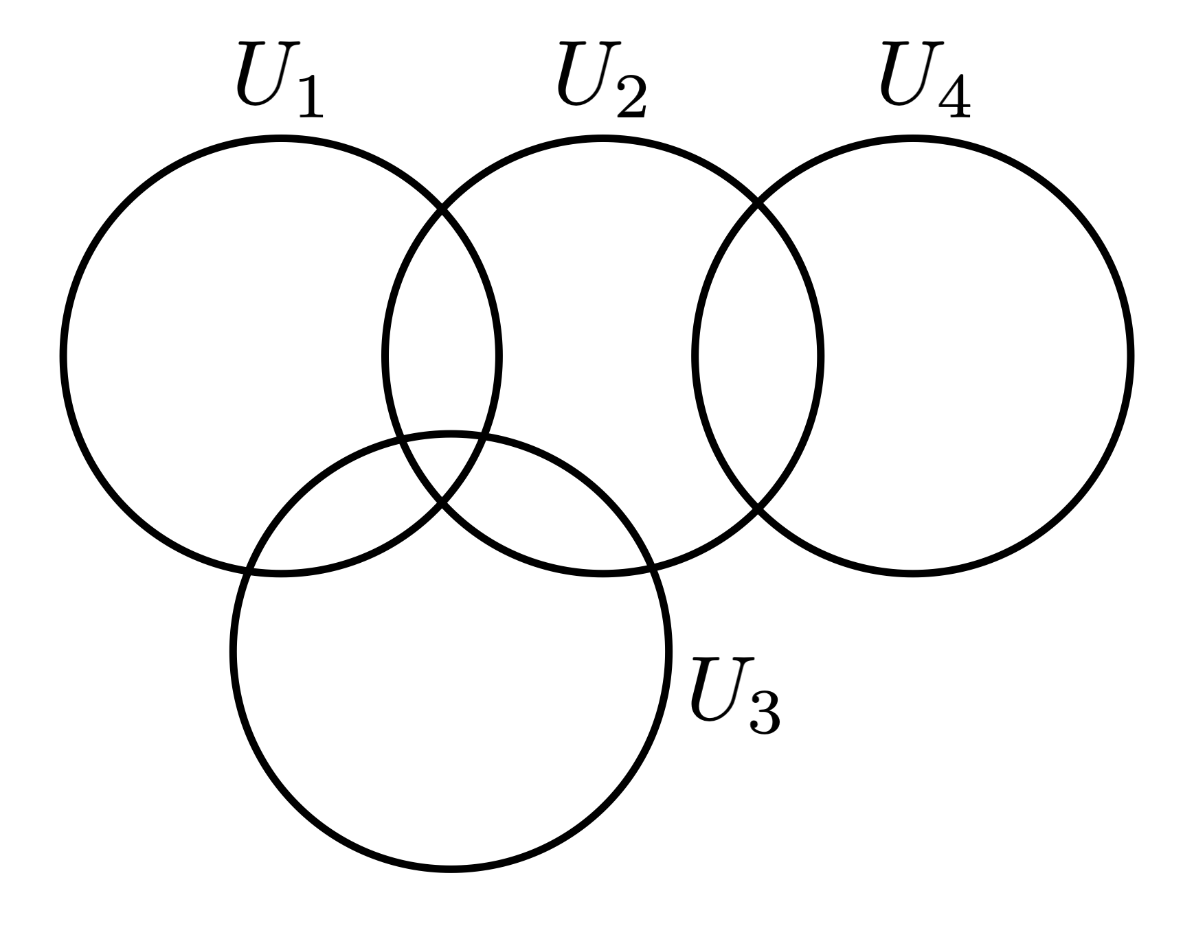
Neural rings were first introduced in [NRingBMB] as an algebraic tool to study receptive field codes (RF codes). RF codes arise in the brain in many contexts. One particular example is place cells - certain cells in the hippocampus that fire consistently every time an animal is in the same location within an environment (the stimulus space) [okeefe]. The set of locations where a particular cell fires is called its place field - or more generally, its receptive field. A neural code consists of a binary codeword for each distinct intersection of receptive fields that appears in the stimulus space (see Figure 2.1.1 for an example). Typically, we consider stimulus spaces as subsets of a subspace XX of ℝd\mathbb{R}^{d}; in the case of place cells, d=2d=2 or 33, but there are other types of neurons whose receptive fields naturally lie in different dimensions (see [NRingBMB] and references therein).

The neural ring (and the related neural ideal) provide a tool for applying algebraic methods to these receptive field codes. Roughly speaking, the neural ideal is the set of polynomials that vanish at every codeword of a given neural code, excepting those that vanish on every possible codeword. These polynomials can then be interpreted to give descriptions of relationships between the receptive fields (such as containment or disjointness). This information, in turn, can be used to answer questions about what sort of arrangements of receptive fields could have generated the code.

Some such questions (e.g. could a particular code have arisen from an arrangement of convex, open regions?) are quite difficult to answer for neural codes in general [NCConvex]. However, there are some types of codes that are quickly detectable and/or whose neural ideals have particularly nice generators.

One such collection is inductively pierced codes [GrossObatakeYoungs]. As the name suggests, these are codes that can be constructed iteratively, by adding receptive fields to an existing arrangement following strict conditions on how each receptive field may interact with those already present. These codes are easily detectable from their algebraic signature. They have a strong connection to chordal graphs, and bounds on the best dimension in which an arrangement using convex regions exists are known (and if the receptive fields are spheres, the dimension can be exactly determined)[curry2022recognizing].

One obstruction to computing algebraic invariants of neural ideals is that they are generated by pseudomonomials, products Πi∈σ​xi​Πi∈τ​(1−xi)\Pi_{i\in\sigma}x_{i}\Pi_{i\in\tau}(1-x_{i}), which are neither graded nor local and as a result are not as well studied in commutative algebra. To deal with this issue, Güntürkün, Jeffries, and Sun give a process for polarizing a neural ideal, turning it into a squarefree monomial ideal in the extension ring 𝔽2​[x1,…,xn,y1,…,yn]\mathbb{F}_{2}[x_{1},\ldots,x_{n},y_{1},\ldots,y_{n}] [neuralpolarization]. One can then compute invariants such as Betti numbers for this ideal instead, and they carry over to information on the original neural ideal.

The primary goal of this paper is to compute homological invariants of polarized neural ideals and describe how they correspond to geometric features of the associated arrangement of receptive fields. In particular, we will focus on the Betti numbers for the polarized neural ideals of inductively pierced codes. Broadly, we find that this offers an algebraic invariant that provides geometric features of the code and information about its piercing structure, while remaining efficiently computable. More specifically, homological notions such as regularity and Betti numbers can be used to determine whether a neural code is inductively pierced, and if it is, how many piercings of each order it has. If we use a multigrading that tracks degrees in xx’s and yy’s separately, the multigraded Betti numbers can further distinguish how many firing fields each piercing is contained in. This demonstrates that homological invariants have the potential to be extremely useful in classifying neural codes.

The Castelnuovo–Mumford regularity of a homogeneous ideal measures its homological complexity. In particular, among nondegenerate ideals (those containing no linear forms), ideals of regularity 2 are precisely those whose higher-order relations are generated by linear syzygies. Our main results show a neural ideal is quadratic with regularity 2 if and only if the corresponding neural code is inductively pierced (Theorem 3.2). We also compute the Betti numbers (Theorem 4.9 and Corollary 4.10) and projective dimension (Corollary 4.14) of inductively pierced codes. Further, we prove the Betti numbers of an inductively pierced code uniquely determine how many kk-piercings the code has for each kk, implying that the numbers of kk-piercings are an invariant of the code (Corollary 4.11 and Theorem 4.12). Consequently, we prove that the elimination ordering on a chordal graph has a fixed number of each type of simplicial vertex (Theorem 5.5).

Since we expect readers of this paper to have varied mathematical backgrounds, we have included appendices on some of the algebraic and combinatorial background material.

2. Definitions

2.1. Neural codes/rings

Here, we introduce the basic algebraic objects of interest: neural codes and neural rings. Unless otherwise noted, the definitions and results in this section are from [NRingBMB].

We will generally assume we have a set of neurons ii, each of which fires in a particular open set UiU_{i} in some affine space ℝd\mathbb{R}^{d}.

Notation 2.1.

We represent the set of neurons as [n]={1,…,n}[n]=\{1,...,n\}; the power set of [n][n] is denoted 2[n]2^{[n]}.

𝔽2\mathbb{F}_{2} will be the field on two elements.

Definition 2.2.

A neural code 𝒞\mathcal{C} is any collection of subsets of the set [n][n] of all neurons:

𝒞⊆2[n].\mathcal{C}\subseteq 2^{[n]}.

Each element σ\sigma of the code is called a codeword and may be supposed to represent a data point where the neurons in σ\sigma were simultaneously active. As a convention, the element ∅\emptyset is always included in 𝒞\mathcal{C}.

Definition 2.3.

A collection of regions 𝒰={U1,…,Un}\mathcal{U}=\{U_{1},...,U_{n}\} where Ui⊂ℝdU_{i}\subset\mathbb{R}^{d} is a realization of the code 𝒞⊂2[n]\mathcal{C}\subset 2^{[n]} if

𝒞={σ⊆[n]|⋂i∈σUi\⋃j∉σUj≠∅}.\mathcal{C}=\{\sigma\subseteq[n]\,|\,\bigcap_{i\in\sigma}U_{i}\backslash\bigcup_{j\notin\sigma}U_{j}\neq\emptyset\}.
Example 2.4.

Consider the code 𝒞={∅,1,2,3,4,12,14,23,24,35,124,235}\mathcal{C}=\{\emptyset,1,2,3,4,12,14,23,24,35,124,235\} Note that here we use the shorthand of writing, e.g., 123 instead of {1,2,3}\{1,2,3\}. Figure 2.1.1 shows one possible realization of this code.

Refer to caption
Figure 2.1.1. A realization of the code 𝒞\mathcal{C} from Example 2.4. The region corresponding to codeword 2323 is highlighted.
Definition 2.5.

Given a neural code on nn neurons, we consider the associated ideal

I​(𝒞)={f∈R|f​(c)=0​∀c∈𝒞}I(\mathcal{C})=\{f\in R\,|\,f(c)=0\,\forall\,c\in\mathcal{C}\}

of R=𝔽2​[x1,…,xn]R=\mathbb{F}_{2}[x_{1},\ldots,x_{n}], where ff is evaluated at cc by inputting a 1 for xix_{i} if i∈ci\in c and a 0 for xix_{i} otherwise.

The neural ring is defined to be

R𝒞=R/I​(𝒞).R_{\mathcal{C}}=R/I(\mathcal{C}).

The ideal I​(𝒞)I(\mathcal{C}) can be decomposed into two parts:

I​(𝒞)=B+LI(\mathcal{C})=B+L

where

B=(x1​(1−x1),…,xn​(1−xn)),B=\left(x_{1}(1-x_{1}),...,x_{n}(1-x_{n})\right),

and

L=(ρv|v∈2[n]\𝒞)L=\left(\rho_{v}\,|\,v\in 2^{[n]}\backslash\mathcal{C}\right)

where ρv=∏i∈vxi​∏j∉v(1−xj)\rho_{v}=\prod_{i\in v}x_{i}\prod_{j\notin v}(1-x_{j}). Note that BB is always the same, and reflects the use of the finite field 𝔽2\mathbb{F}_{2}, whereas the ideal LL is specific to the particular code 𝒞\mathcal{C}. Thus, we will focus mostly on the properties of LL, which we title the neural ideal.111In much of the literature, the notation for the neural ideal is JJ instead of LL. However, as we will rarely consider the neural ideal LL itself in this paper, we reserve JJ for other uses (namely, its polarized version).

Definition 2.6.

A pseudo-monomial is a polynomial f∈Rf\in R of the form f=∏i∈σxi​∏j∈τ(1−xj)f=\prod_{i\in\sigma}x_{i}\prod_{j\in\tau}(1-x_{j}), where σ∩τ=∅\sigma\cap\tau=\emptyset.

Observe that LL is generated by pseudo-monomials. In fact, these generators are, in a sense, maximal – if we multiply them by any linear factor xix_{i} or 1−xi1-x_{i} not already part of the product, they would also be part of BB, and thus redundant. The minimal pseudo-monomials of LL are more interesting, and provide another useful generating set for LL.

Definition 2.7.

The canonical form of a code 𝒞\mathcal{C}, denoted C​F​(𝒞)CF(\mathcal{C}), is the set of all minimal pseudo-monomials of LL, where a pseudo-monomial ff is said to be minimal if no other pseudo-monomial gg of LL divides ff. If LL is the neural ideal of 𝒞\mathcal{C}, we may also refer to the canonical form of 𝒞\mathcal{C} as C​F​(L)CF(L) without explicitly listing 𝒞\mathcal{C}.

The canonical form generates the ideal LL (that is, L=(C​F​(𝒞))L=(CF(\mathcal{C}))) and is often a friendlier collection of generators than the set ρv\rho_{v}.

Example 2.8.

Observe that the code 𝒞\mathcal{C} from Example 2.4 is a code on five neurons, with twelve codewords. If we use the generators ρv\rho_{v} for LL as in Definition 2.5 then LL would have 25−12=202^{5}-12=20 generators ρv\rho_{v}, each of degree 5. For example, as v=145v=145 is not in 𝒞\mathcal{C}, then ρ145=x1​x4​x5​(1−x2)​(1−x3)\rho_{145}=x_{1}x_{4}x_{5}(1-x_{2})(1-x_{3}) would be one such generator.

The canonical form (Definition 2.7), however, is much simpler. In this case, it contains only five pseudo-monomials, all of degree two:

C​F​(𝒞)={x1​x3,x1​x5,x3​x4,x4​x5,x5​(1−x3)}.CF(\mathcal{C})=\{x_{1}x_{3},\,x_{1}x_{5},\,x_{3}x_{4},\,x_{4}x_{5},\,x_{5}(1-x_{3})\}.
Remark 2.9.

Because the canonical form by definition contains all minimal pseudo-monomials, it may not be the shortest possible list of generators. For example, the code 𝒞={∅,1,12,123}\mathcal{C}=\{\emptyset,1,12,123\} has canonical form

C​F​(𝒞)={x3​(1−x2),x2​(1−x1),x3​(1−x1)}.CF(\mathcal{C})=\{x_{3}(1-x_{2}),x_{2}(1-x_{1}),x_{3}(1-x_{1})\}.

But the ideal LL can also be generated by the shorter list {x3​(1−x2),x2​(1−x1)}\{x_{3}(1-x_{2}),x_{2}(1-x_{1})\}, since x3​(1−x1)=(1−x1)​[x3​(1−x2)]+x3​[x2​(1−x1)]x_{3}(1-x_{1})=(1-x_{1})[x_{3}(1-x_{2})]+x_{3}[x_{2}(1-x_{1})].

Neural ideals were originally studied using these pseudo-monomials; however, since they are neither standard graded nor all contained in any maximal ideal, many algebraic invariants do not apply. Instead, we convert neural ideals to monomial ideals using an operation called polarization. Monomial ideals are graded under the standard grading, or many multi-gradings, so we can compute homological invariants like Betti numbers for them.

Notation 2.10.

Throughout this paper, except where otherwise specified, R:=𝔽2​[x1,…,xn]R:=\mathbb{F}_{2}[x_{1},\ldots,x_{n}] will be the polynomial ring on nn variables, and

S:=𝔽2​[x1,…,xn,y1,…,yn]S:=\mathbb{F}_{2}[x_{1},\ldots,x_{n},y_{1},\ldots,y_{n}]

will be the polynomial ring on 2​n2n variables. By default, both rings will be standard graded, except where a multi-grading is explicitly given. Neural ideals on nn neurons will live in RR and polarized neural ideals on nn neurons (which are graded) will live in SS. All Betti numbers (see Appendix A for definitions) will be computed over SS unless otherwise noted.

Definition 2.11 ([neuralpolarization]*Section 3).

We define a polarization function 𝒫\mathcal{P} (not a homomorphism) that sends pseudo-monomials in RR to squarefree monomials in SS via

∏i∈σxi​∏i∈τ(1−xi)↦∏i∈σxi​∏i∈τyi.\prod_{i\in\sigma}x_{i}\prod_{i\in\tau}(1-x_{i})\mapsto\prod_{i\in\sigma}x_{i}\prod_{i\in\tau}y_{i}.

This does not extend to a ring homomorphism.

If II is an ideal of RR, then 𝒫​(I)\mathcal{P}(I) is the ideal of SS generated by 𝒫​(f)\mathcal{P}(f) for all pseudo-monomials f∈If\in I.

We also define a depolarization map d:S→Rd:S\to R, which is the ring homomorphism sending xi↦xi,yi↦1−xix_{i}\mapsto x_{i},y_{i}\mapsto 1-x_{i}. The map dd induces an isomorphism of SS-modules S/(∑i=1n(xi+yi−1))≅RS/\left(\sum_{i=1}^{n}(x_{i}+y_{i}-1)\right)\cong R.

Theorem 2.12 ([neuralpolarization]*Theorem 3.2).

Let {g1,…,gk}⊆R\{g_{1},\ldots,g_{k}\}\subseteq R be the canonical form of a neural ideal LL. Then 𝒫​(L)=(𝒫​(g1),…,𝒫​(gk))\mathcal{P}(L)=(\mathcal{P}(g_{1}),\ldots,\mathcal{P}(g_{k})).

Definition 2.13.

The polarized canonical form of a neural ideal is the list {𝒫​(g1),…,𝒫​(gk)}⊆S\{\mathcal{P}(g_{1}),\ldots,\mathcal{P}(g_{k})\}\subseteq S, where {g1,…,gk}⊆R\{g_{1},\ldots,g_{k}\}\subseteq R is the canonical form of a neural ideal LL. We will often refer to the polarized canonical form of a neural ideal without specifying LL, but LL can be found by depolarizing the elements of the polarized canonical form.

We will refer to the ideal JJ of SS generated by the polarized canonical form of a neural ideal as the polarized neural ideal. This is a squarefree monomial ideal, so it is graded.

One of the primary goals of this paper is to classify neural ideals by their canonical resolutions.

Definition 2.14 ([neuralpolarization]*Definition 4.5).

Let L⊆RL\subseteq R be a neural ideal with canonical form C​F​(L)CF(L), and J⊆SJ\subseteq S its polarized neural ideal . The canonical resolution of LL is G∙=F∙⊗SS/(x1+y1−1,…,xn+yn−1)G_{\bullet}=F_{\bullet}\otimes_{S}S/(x_{1}+y_{1}-1,\ldots,x_{n}+y_{n}-1), where F∙F_{\bullet} is a minimal free resolution of JJ over SS (which exists because S/JS/J is graded).

Remark 2.15.

Since this construction involves taking a quotient by a regular sequence, G∙G_{\bullet} is a resolution of R/LR/L by Corollary A.7. Further, the canonical resolution G∙G_{\bullet} of LL has the same numbers of copies of RR in each homological degree as F∙F_{\bullet} has copies of SS, and the maps ∂∙G\partial_{\bullet}^{G} are given by replacing each yiy_{i} from the corresponding map ∂∙F\partial_{\bullet}^{F} by 1−xi1-x_{i}, also by Corollary A.7.

As a result, the Betti numbers of JJ give us the shape of the canonical resolution of LL. We will primarily discuss the resolution of JJ over SS, so as to be able to use terms like “Betti numbers”, but we will still gain information on the canonical resolution.

Consequently, we make the following definition:

Definition 2.16.

Given Remark 2.15, we define the Betti numbers of a neural code 𝒞\mathcal{C} by setting βi​(𝒞)\beta_{i}(\mathcal{C}) to be the number of copies of RR in the iith homological degree of the canonical resolution of 𝒞\mathcal{C}.

Lemma 2.17.

Let J=(g1,…,gk)J=(g_{1},\ldots,g_{k}) be a polarized neural ideal , i.e.

𝒫​(C​F​(L))={g1,…,gk}\mathcal{P}(CF(L))=\{g_{1},\ldots,g_{k}\}

for some neural ideal L⊆RL\subseteq R. Then {g1,…,gk}\{g_{1},\ldots,g_{k}\} is a minimal generating set for JJ.

Proof.

By Proposition 1.3.5 of [monomialideals], this is a minimal generating set if and only if it is irredundant, i.e. no gig_{i} is divisible by any gjg_{j} for j≠ij\neq i. But this is true as no element of C​F​(L)CF(L) divides any other, and by [neuralpolarization]*Lemma 3.1 polarization preserves this property. ∎

2.2. Inductively Pierced Codes

The literature on neural codes is considerable and addresses many questions - which codes are convex? In what dimension? How can these codes be detected? (See [NCConvex, NRingBMB] and related literature.) These questions typically do not have simple answers. However, many classes of codes have been identified that do have nice properties, some of which are easy to detect. One such class of codes is those that are inductively pierced. Informally, a code is inductively pierced if it can be constructed iteratively, by adding new neurons to the code to interact with existing neurons only in restricted and predictable ways. To formally define these codes, we need to build up a bit of notation. The following definitions are from [curry2022recognizing], but note that we have rephrased any algebraic results to use the polarized form of the neural ideal.

Definition 2.18.

For any σ⊆τ⊆[n]\sigma\subseteq\tau\subseteq[n], the interval between σ\sigma and τ\tau is the set

[σ,τ]={γ⊆[n]∣σ⊆γ⊆τ}.[\sigma,\tau]=\{\gamma\subseteq[n]\mid\sigma\subseteq\gamma\subseteq\tau\}.

The rank of an interval [σ,τ][\sigma,\tau] is equal to |τ|−|σ||\tau|-|\sigma|.

Definition 2.19.

Given a code 𝒞⊆2[n]\mathcal{C}\subseteq 2^{[n]} and a neuron i∈[n]i\in[n], we can construct the code 𝒞\i\mathcal{C}\backslash i, called the deletion of ii, which is obtained by deleting ii from every codeword in 𝒞\mathcal{C} where it appears. For any σ⊆[n]\sigma\subseteq[n], we let 𝒞\σ\mathcal{C}\backslash\sigma denote the code obtained by deleting all neurons i∈σi\in\sigma from 𝒞\mathcal{C}.

Definition 2.20.

Let 𝒞⊆2[n]\mathcal{C}\subseteq 2^{[n]} be a code and let i∈[n]i\in[n] be a neuron. We say that ii is an (abstract) kk-piercing of 𝒞\mathcal{C} if there exist σ⊆τ⊆[n]\{i}\sigma\subseteq\tau\subseteq[n]\backslash\{i\} so that [σ,τ][\sigma,\tau] has rank kk and the following two conditions are satisfied:

  • (i)

    [σ,τ][\sigma,\tau] is contained in 𝒞\i\mathcal{C}\backslash i, and

  • (ii)

    𝒞=(𝒞\i)∪[σ∪{i},τ∪{i}]\mathcal{C}=(\mathcal{C}\backslash i)\cup[\sigma\cup\{i\},\tau\cup\{i\}].

More informally, to have a kk-piercing, every element of this interval of rank kk must appear both with and without ii, and these must be the only appearances of ii. If we think of this from the perspective of a realization, the region UiU_{i} is contained within UσU_{\sigma}, all of the neurons in τ\σ\tau\backslash\sigma appear in all combinations within UσU_{\sigma}, and all of the neurons in (τ\σ)∪{i}(\tau\backslash\sigma)\cup\{i\} appear in all combinations within UσU_{\sigma}.

The above definition tells us how to identify if a given neuron is a kk-piercing of the others. More often, however, we are interested in building up a code by adding neurons in succession so that each is a kk-piercing of the ones that precede it. Codes that can be built this way are called inductively pierced.

Definition 2.21.

A code 𝒞⊆2[n]\mathcal{C}\subseteq 2^{[n]} is kk-inductively pierced if 𝒞={∅}\mathcal{C}=\{\emptyset\}, or there exists a neuron i∈[n]i\in[n] which is a k′k^{\prime}-piercing of 𝒞\mathcal{C} for some k′≤kk^{\prime}\leq k, and 𝒞\i\mathcal{C}\backslash i is kk-inductively pierced.

By the iterative nature of this definition, any inductively pierced code must have an ordering i1<i2<⋯<ini_{1}<i_{2}<\cdots<i_{n} of the neurons [n][n] so that for each jj, the neuron iji_{j} is a k′k^{\prime}-piercing of the code 𝒞\{ij+1,…,in}\mathcal{C}\backslash\{i_{j+1},\ldots,i_{n}\} for some k′≤kk^{\prime}\leq k. We call such an order a piercing order.

In general, an inductively pierced code may have many valid piercing orders, and so we do not assume this ordering is unique. Example 2.22 provides a code with multiple possible piercing orders. These orders do share some properties, which we list here.

  1. (1)

    For any k′k^{\prime}, a k′k^{\prime}-piercing can only be constructed on a k′−1k^{\prime}-1-piercing. As a result iji_{j} is at most a j−1j-1-piercing, and in particular i1i_{1} is a 0-piercing.

  2. (2)

    Any two piercing orders for the same code contain the same number of k′k^{\prime} piercings, for any k′≤kk^{\prime}\leq k. We will prove this result later (see Corollary 4.11).
Refer to caption
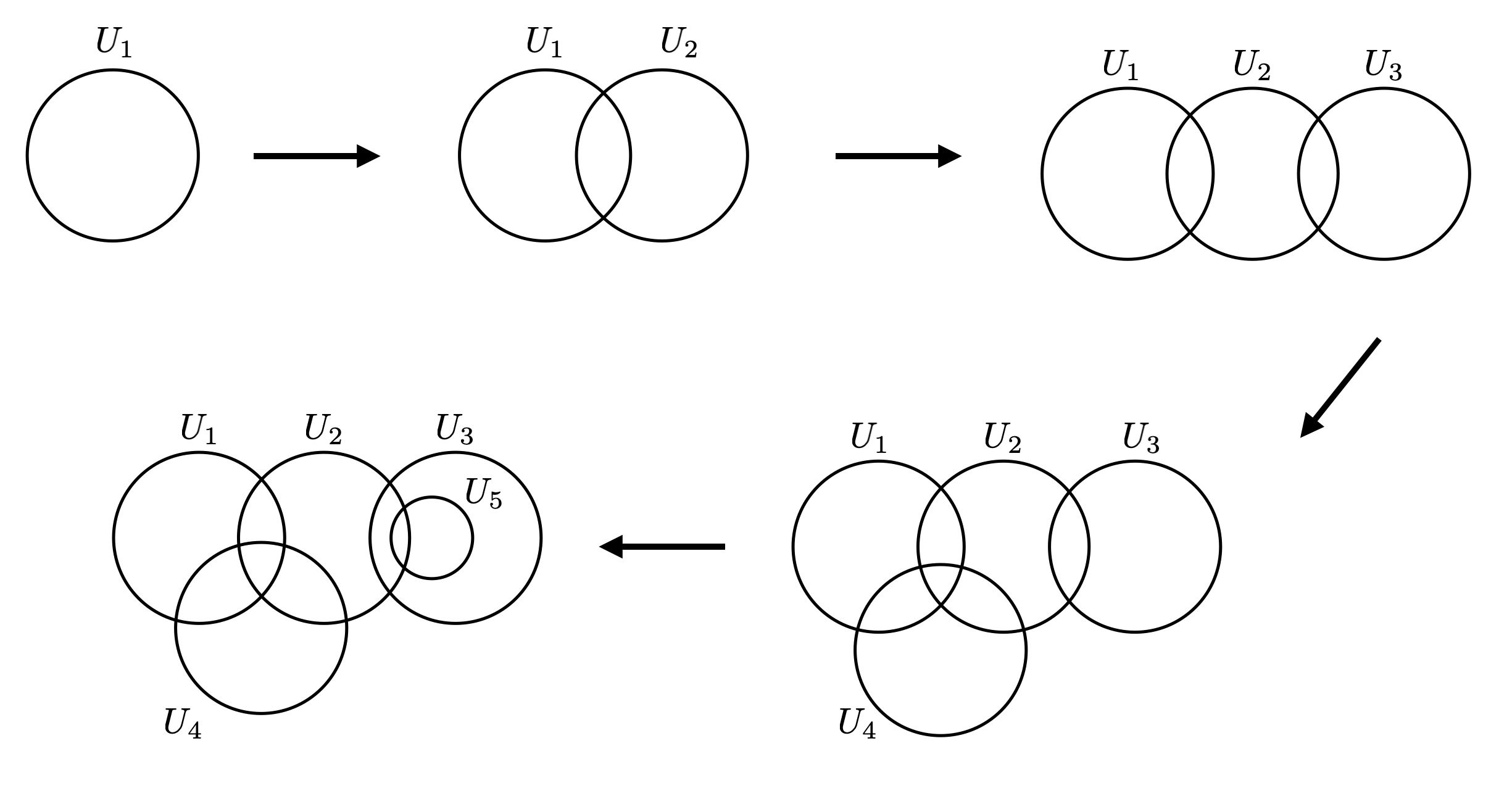
Figure 2.2.1. Building the code from Example 2.22 from the piercing order 1,2,3,4,5.
Example 2.22.

The code 𝒞\mathcal{C} from Example 2.4 is inductively pierced. We can build the code using a succession of piercings as follows (see Figure 2.2.1):

First, start with 𝒞0={∅}\mathcal{C}_{0}=\{\emptyset\}; this is inductively pierced by definition.

We then can take code 𝒞1={∅,1}\mathcal{C}_{1}=\{\emptyset,1\}, where neuron 1 is a 0-piercing (in this case, σ=τ=∅\sigma=\tau=\emptyset). Note that 𝒞1\1=𝒞0\mathcal{C}_{1}\backslash 1=\mathcal{C}_{0}.

The code 𝒞2={∅,1,2,12}\mathcal{C}_{2}=\{\emptyset,1,2,12\} has neuron 2 as a 1-piercing (where σ=∅\sigma=\emptyset, τ=1\tau=1). Here, 𝒞2\2=𝒞1\mathcal{C}_{2}\backslash 2=\mathcal{C}_{1}.

The code 𝒞3={∅,1,2,3,12,23}\mathcal{C}_{3}=\{\emptyset,1,2,3,12,23\} has neuron 3 as another 1-piercing (with σ=∅\sigma=\emptyset, τ=2\tau=2). Here, 𝒞3\3=𝒞2\mathcal{C}_{3}\backslash 3=\mathcal{C}_{2}.

The code 𝒞4={∅,1,2,3,4,12,23,14,24,124}\mathcal{C}_{4}=\{\emptyset,1,2,3,4,12,23,14,24,124\} contains neuron 44 as a 2-piercing of 11 and 22 (so σ=∅,τ=12)\sigma=\emptyset,\tau=12). Here, 𝒞4\4=𝒞3\mathcal{C}_{4}\backslash 4=\mathcal{C}_{3}.

And finally, the code 𝒞5=𝒞={∅,1,2,3,4,12,23,14,24,35,124,235}\mathcal{C}_{5}=\mathcal{C}=\{\emptyset,1,2,3,4,12,23,14,24,35,124,235\} has 55 as a 1-piercing of 2 (within 33), so σ=3\sigma=3 and τ=23\tau=23. Here, 𝒞\5=𝒞4\mathcal{C}\backslash 5=\mathcal{C}_{4}.

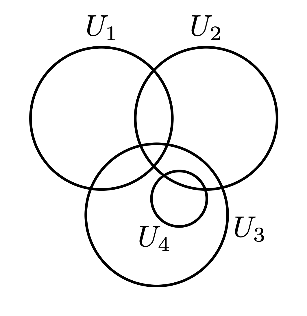
The piercing order in this case is the same as the labels: 1,2,3,4,5. However, the code can also be built using the order 1,4,2,3,51,4,2,3,5 as depicted in Figure 2.2.2 –note that in this case, neuron 44 would be a 1-piercing with τ=1\tau=1, but 22 would now be a 2−2-piercing with τ=12\tau=12.

However, not all orders are valid piercing orders - for example, 5,3,1,2,45,3,1,2,4 is not valid as 33 is not a piercing (of any order) of the code consisting of only neuron 55.

Refer to caption
Figure 2.2.2. Building the code from Example 2.22 in the label order 1,4,2,3,5.

Inductively pierced codes are detectable using the canonical form and an associated graph. This result (and the related definitions) are from [curry2022recognizing], but we provide it in its polarized form, since that is the form in which we will use it. We note that polarization preserves the degrees of the generators of the canonical form, and the polarized neural ideal of a neural code 𝒞\mathcal{C} contains a binomial xi​xjx_{i}x_{j} (resp. xi​yjx_{i}y_{j}, xj​yix_{j}y_{i}, yi​yjy_{i}y_{j}) if and only if the canonical form of 𝒞\mathcal{C} contains xi​xjx_{i}x_{j} (resp. xi​(1−xj)x_{i}(1-x_{j}), xj​(1−xi)x_{j}(1-x_{i}), (1−xi)​(1−xj)(1-x_{i})(1-x_{j})), so polarization preserves the properties relevant to these results. For this theorem, we need two additional definitions:

Definition 2.23.

Let 𝒞\mathcal{C} be a code on nn neurons that has a degree two canonical form. The general relationship graph G​(𝒞)G(\mathcal{C}) is the graph with vertices V=[n]V=[n], and an edge i,j{i,j} if and only if the polarized neural ideal JJ of 𝒞\mathcal{C} does not contain any of the pseudo-monomials xi​xjx_{i}x_{j}, xi​yjx_{i}y_{j}, xj​yix_{j}y_{i}.

[Note: because of the convention ∅∈𝒞\emptyset\in\mathcal{C}, the monomial yi​yjy_{i}y_{j} never appears in any polarized neural ideal .]

Definition 2.24.

A graph GG is chordal if it has no chordless cycle (every cycle of length ≥4\geq 4 has a chord) [West]*Definition 5.3.12.

One notable property of chordal graphs is that they can be built up iteratively by adding so-called simplicial vertices; the similarity of inductive construction is not accidental.

Theorem 2.25 ([curry2022recognizing]*Theorem 6).

A neural code 𝒞\mathcal{C} is inductively pierced if and only if

  1. (1)

    C​F​(𝒞)CF(\mathcal{C}) consists of degree two polynomials and

  2. (2)

    the graph G​(𝒞)G(\mathcal{C}) is chordal.

Since determining whether a graph is chordal is relatively efficient, this result allows us to realistically detect whether a code is inductively pierced. Other results in [curry2022recognizing] prove that such codes are always realizable using convex sets, and provide upper bounds on the minimum dimension required to build such a realization.

Remark 2.26.

The result as stated is only for strictly degree-two canonical forms. However, for practical purposes, degree-one terms can usually be dealt with via a minor modification of the code. The term yiy_{i} is impossible due to the requirement that 𝒞\mathcal{C} contain the empty set. The term xix_{i} would indicate that neuron ii never appears in any set in 𝒞\mathcal{C}; in this case, we can replace 𝒞\mathcal{C} with 𝒞\i\mathcal{C}\backslash i and eliminate the problem altogether, without changing any important property of the original code.

Technically, the original result also requires that the canonical form contains at most one degree-two term for each pair i,ji,j. However, due to properties of the canonical form, most combinations of such terms cannot possibly appear in the canonical form anyway. The one combination which can occur (xi​yjx_{i}y_{j} and xj​yix_{j}y_{i}) would indicate that neurons ii and jj are identical in 𝒞\mathcal{C}, and so we can work with an equivalent code where we replace both with one single neuron. In this paper, we typically assume that this situation does not occur.

3. Homological Invariants of Inductively Pierced Codes

In this section, we leverage Theorem 3.2 to compute common homological invariants of SS modules, namely, Betti numbers and regularity. For background, see Appendix A. We include in this section some background on multi-gradings and their associated homological invariants.

Notation 3.1.

Throughout this section, 𝒞\mathcal{C} will be a neural code on nn neurons, nn will be a kk-piercing of 𝒞\{n}\mathcal{C}\backslash\{n\} (the code obtained by deleting nn from 𝒞\mathcal{C}), and JnJ_{n} will be the polarized neural ideal of 𝒞\mathcal{C} in S=𝔽2​[x1,…,xn,y1,…,yn]S=\mathbb{F}_{2}[x_{1},\ldots,x_{n},y_{1},\ldots,y_{n}]. We let Jn−1J_{n-1} denote the polarized neural ideal of 𝒞\{n}\mathcal{C}\backslash\{n\}, expanded to SS since this does not impact the homological invariants studied here. We will assume all other ideals discussed live in SS unless otherwise specified.

First we give a homological characterization of inductively pierced codes, which can be viewed as adding a condition to Theorem 2.25.

Theorem 3.2.

Let 𝒞\mathcal{C} be a neural code on nn neurons and JJ its polarized neural ideal contained in S=𝔽2​[x1,…,xn,y1,…,yn]S=\mathbb{F}_{2}[x_{1},\ldots,x_{n},y_{1},\ldots,y_{n}]. Assume that:

  1. (1)

    the canonical form of JJ is generated by quadratic forms,

  2. (2)

    no union of UiU_{i} covers all of XX, and

  3. (3)

    no Ui=UjU_{i}=U_{j} for i≠ji\neq j.

Then 𝒞\mathcal{C} is inductively pierced if and only if reg⁡(J)=2\operatorname{reg}\left({J}\right)=2.

Remark 3.3.

Notice that the listed conditions (1)-(3) imply that for each pair i,ji,j, JJ has at most one generator chosen from xi​xjx_{i}x_{j}, xi​yjx_{i}y_{j}, and xj​yix_{j}y_{i}. Further, these are the only generators of JJ.

To prove this result, we need the following lemma. See Definition A.5 for the definition of a regular sequence.

Lemma 3.4.

Let 𝒞\mathcal{C} be a neural code on nn neurons and JJ its polarized neural ideal contained in S=𝔽2​[x1,…,xn,y1,…,yn]S=\mathbb{F}_{2}[x_{1},\ldots,x_{n},y_{1},\ldots,y_{n}]. Assume the hypotheses (1)-(3) of Theorem 3.2. Then the sequence (x1−y1,…,xn−yn)(x_{1}-y_{1},\ldots,x_{n}-y_{n}) is S/JS/J-regular.

Proof.

Since JJ is square-free and a neural ideal, no generator of JJ is divisible by xi​yix_{i}y_{i} for all 1≤i≤n1\leq i\leq n and we obtain the ideals 𝔑i\mathfrak{N}_{i}, 𝔛i\mathfrak{X}_{i}, and 𝔛i\mathfrak{X}_{i} satisfying

J=𝔑i+𝔛i​xi+𝔜i​yiJ=\mathfrak{N}_{i}+\mathfrak{X}_{i}x_{i}+\mathfrak{Y}_{i}y_{i}

where xix_{i} and yiy_{i} do not divide any generator of 𝔑i\mathfrak{N}_{i}, 𝔛i\mathfrak{X}_{i}, and 𝔜i\mathfrak{Y}_{i}. By [GellerRG]*Theorem 5.5, we have 𝔛i∩𝔜i⊆J\mathfrak{X}_{i}\cap\mathfrak{Y}_{i}\subseteq J for all 1≤i≤n1\leq i\leq n. We also find that the images 𝔛i\mathfrak{X}_{i} and 𝔜i\mathfrak{Y}_{i} in S/JS/J, denoted 𝔛i¯\overline{\mathfrak{X}_{i}} and 𝔜i¯\overline{\mathfrak{Y}_{i}} respectively, satisfy

𝔛i¯=AnnS/J⁡(xi) and 𝔜i¯=AnnS/J⁡(yi).\overline{\mathfrak{X}_{i}}=\operatorname{Ann}_{S/J}\!\left({x_{i}}\right)\quad\text{ and }\quad\overline{\mathfrak{Y}_{i}}=\operatorname{Ann}_{S/J}\!\left({y_{i}}\right).

Since 𝔛i¯\overline{\mathfrak{X}_{i}} is a square-free monomial ideal, it is equal to its radical and

𝔛i¯=⋂𝔮¯∈SuppS/J⁡(xi¯)𝔮¯=⋂J+𝔛i⊆𝔮⊂S𝔮¯\overline{\mathfrak{X}_{i}}=\bigcap_{\overline{\mathfrak{q}}\in\operatorname{Supp}_{S/J}\!\left(\overline{x_{i}}\right)}\overline{\mathfrak{q}}=\bigcap_{J+\mathfrak{X}_{i}\subseteq\mathfrak{q}\subset S}\overline{\mathfrak{q}}

where SuppS/J⁡(M)\operatorname{Supp}_{S/J}\!\left(M\right) is the set of all primes 𝔮\mathfrak{q} in S/JS/J such that the localization of MM at 𝔮\mathfrak{q} is non-zero, i.e., M𝔮≠0M_{\mathfrak{q}}\neq 0.

Since we are intersecting over all primes containing J+𝔛iJ+\mathfrak{X}_{i}, we may assume without loss of generality that 𝔮\mathfrak{q} is minimal over J+𝔛iJ+\mathfrak{X}_{i}. Since J+𝔛iJ+\mathfrak{X}_{i} is monomial, 𝔮\mathfrak{q} is also monomial, meaning xi−yi∈𝔮x_{i}-y_{i}\in\mathfrak{q} if and only if xi,yi∈𝔮x_{i},y_{i}\in\mathfrak{q}. Combining the fact that 𝔮\mathfrak{q} is minimal and xix_{i} does not divide any generators of J+𝔛iJ+\mathfrak{X}_{i}, we find xi∉𝔮x_{i}\notin\mathfrak{q} and thus xi−yi∉𝔮x_{i}-y_{i}\notin\mathfrak{q}. Now consider s∈Ss\in S such that s​(xi−yi)∈J⊂𝔮s(x_{i}-y_{i})\in J\subset\mathfrak{q}. Since qq is prime, we find s∈𝔮s\in\mathfrak{q}, allowing us to conclude that for all s¯∈S/J\overline{s}\in S/J satisfying s¯​(xi−yi¯)=0¯\overline{s}(\overline{x_{i}-y_{i}})=\overline{0} in S/JS/J, we have s¯∈𝔮¯\overline{s}\in\overline{\mathfrak{q}}. This tells us that xi¯\overline{x_{i}} and yi¯\overline{y_{i}} correspond to distinct equivalence classes of (S/J)𝔮¯(S/J)_{\overline{\mathfrak{q}}} and thus (xi−yi¯)𝔮¯≠0(\overline{x_{i}-y_{i}})_{\overline{\mathfrak{q}}}\neq 0. This demonstrates that

AnnS/J⁡(xi−yi¯)⊆⋂𝔮¯∈SuppS/J⁡(xi¯)𝔮¯=𝔛i¯.\operatorname{Ann}_{S/J}\!\left({\overline{x_{i}-y_{i}}}\right)\subseteq\bigcap_{\overline{\mathfrak{q}}\in\operatorname{Supp}_{S/J}\!\left(\overline{x_{i}}\right)}\overline{\mathfrak{q}}=\overline{\mathfrak{X}_{i}}.

An analogous argument shows AnnS/J⁡(xi−yi¯)⊆𝔜i¯.\operatorname{Ann}_{S/J}\!\left({\overline{x_{i}-y_{i}}}\right)\subseteq\overline{\mathfrak{Y}_{i}}. Combining these two results gives

AnnS/J⁡(xi−yi¯)⊆𝔛i¯∩𝔜i¯=𝔛i∩𝔜i¯⊆J¯=0,\operatorname{Ann}_{S/J}\!\left({\overline{x_{i}-y_{i}}}\right)\subseteq\overline{\mathfrak{X}_{i}}\cap\overline{\mathfrak{Y}_{i}}=\overline{\mathfrak{X}_{i}\cap\mathfrak{Y}_{i}}\subseteq\overline{J}=0,

that is, xi−yi¯\overline{x_{i}-y_{i}} is a non-zero divisor in S/JS/J. Moreover, xi−yi¯\overline{x_{i}-y_{i}} is not a unit in S/JS/J since the only unit is 1. Thus xi−yi¯\overline{x_{i}-y_{i}} is a regular element in S/JS/J, and xi−yix_{i}-y_{i} is (S/J)(S/J)-regular for all 1≤i≤n1\leq i\leq n.

Specifically, x1−y1x_{1}-y_{1} is (S/J)(S/J)-regular. For i>1i>1, set

Mi:=SJ(x1−y1,…,xi−1−yi−1)​SJ≅𝔽2​[x1,…,xn,yi,…,yn]J(i)M_{i}:=\frac{\frac{S}{J}}{(x_{1}-y_{1},\ldots,x_{i-1}-y_{i-1})\frac{S}{J}}\cong\frac{\mathbb{F}_{2}[x_{1},\ldots,x_{n},y_{i},\ldots,y_{n}]}{J_{(i)}}

where J(i)J_{(i)} is the image of JJ with each y1,…,yi−1y_{1},\ldots,y_{i-1} replaced with x1,…,xi−1x_{1},\ldots,x_{i-1}, respectively. The proof that xi−yi¯\overline{x_{i}-y_{i}} is a regular element in MiM_{i}, viewed as a ring, is identical to the proof that xi−yi¯\overline{x_{i}-y_{i}} is a regular element in S/JS/J. This shows that xi−yix_{i}-y_{i} is MiM_{i}-regular for each i>1i>1, implying that the sequence x1−y1,…,xn−ynx_{1}-y_{1},\ldots,x_{n}-y_{n} is (S/J)(S/J)-regular. ∎

We now prove Theorem 3.2.

Proof of Theorem 3.2.

By our hypotheses, every generator of the canonical form of JJ is of the form xi​xjx_{i}x_{j} or xi​yjx_{i}y_{j} for some i,ji,j. If for some fixed ii and jj, we have both xi​xjx_{i}x_{j} and xi​yjx_{i}y_{j}, then the canonical form has a generator dividing xix_{i} by [GellerRG]*Algorithm 5.9, contradicting our hypothesis that the canonical form consists of quadratics. If for some fixed ii and jj, we have both xi​yjx_{i}y_{j} and xj​yix_{j}y_{i}, then Ui=UjU_{i}=U_{j}, contradicting our other hypothesis. Hence for any pair i,ji,j, we have at most one generator chosen from the set {xi​xj,xi​yj,xj​yi}\{x_{i}x_{j},x_{i}y_{j},x_{j}y_{i}\}.

Consequently, we can draw the general relationship graph 𝒢​(𝒞)\mathcal{G}(\mathcal{C}) of 𝒞\mathcal{C} as in [curry2022recognizing], with a vertex for each neuron and an edge connecting vertices ii and jj if JJ has no generator from the set {xi​xj,xi​yj,xj​yi}\{x_{i}x_{j},x_{i}y_{j},x_{j}y_{i}\}. The neural code 𝒞\mathcal{C} is inductively pierced if and only if this graph is chordal by Theorem 2.25.

If every generator of the canonical form is of the form xi​xjx_{i}x_{j}, then JJ is the edge ideal of the complement of 𝒢​(𝒞)\mathcal{G}(\mathcal{C}). By [froberg]*Theorem 1 as interpreted in [banerjee]*Theorem 6, reg⁡(J)=2\operatorname{reg}\left({J}\right)=2 if and only if 𝒢​(𝒞)\mathcal{G}(\mathcal{C}) is chordal, i.e. if and only if 𝒞\mathcal{C} is inductively pierced.

Otherwise, there exists a yiy_{i} that divides one of the generators of JJ. In this case, set S′=𝔽2​[x1,…,xn]S^{\prime}=\mathbb{F}_{2}[x_{1},\ldots,x_{n}] viewed as an SS-module via the isomorphism with S/(x1−y1,x2−y2,…,xn−yn)S/(x_{1}-y_{1},x_{2}-y_{2},\ldots,x_{n}-y_{n}). By Lemma 3.4, x1−y1,…,xn−ynx_{1}-y_{1},\ldots,x_{n}-y_{n} forms a S/JS/J-regular sequence on S/JS/J. By Corollary A.7, tensoring a minimal free resolution of JJ with this quotient gives a minimal free resolution of the ideal J⊗SS′J\otimes_{S}S^{\prime} (over S′S^{\prime}), where the degrees of the maps don’t change. Hence JJ and J⊗SS′J\otimes_{S}S^{\prime} have the same regularity. This ideal will have the same generators as JJ, but with every yiy_{i} replaced by the corresponding xix_{i}. As a result, the new list of generators is in canonical form by [GellerRG]*Theorem 5.5. The corresponding neural code 𝒞′\mathcal{C}^{\prime} will have the same general relationship graph as 𝒢​(𝒞)\mathcal{G}(\mathcal{C}).

By the reasoning in the all xx’s case, J⊗SS′J\otimes_{S}S^{\prime} has regularity 2 over S′S^{\prime} if and only if 𝒢​(𝒞′)=𝒢​(𝒞)\mathcal{G}(\mathcal{C}^{\prime})=\mathcal{G}(\mathcal{C}) is chordal, and hence if and only if 𝒞\mathcal{C} is inductively pierced. Thus JJ has regularity 2 if and only if 𝒞\mathcal{C} is inductively pierced. ∎

Remark 3.5.

Note that if JJ is the polarized neural ideal for some inductively pierced code 𝒞\mathcal{C}, then it is generated by quadratics and, by Theorem 3.2, has regularity 2. This tells us that the minimal free resolution of JJ over SS is linear; that is, if FF is the minimal free resolution JJ over SS then the entries of any matrix representation of the differentials ∂F\partial^{F} are either 0 or linear terms.

This gives detailed information about the Betti and graded Betti numbers of polarized neural ideals.

Remark 3.6.

For our purposes, we are interested in the Betti numbers of S/JS/J instead of the Betti numbers of JJ. Fortunately, one can easily translate between the graded Betti numbers of S/JS/J and JJ by observing that

βi,jS​(S/J)={1i=0=jβi−1,jS​(J)i>00otherise.\beta_{i,j}^{S}\!\left(S/J\right)=\begin{cases}1&i=0=j\\ \beta_{i-1,j}^{S}\!\left(J\right)&i>0\\ 0&\text{otherise}\end{cases}.

In the case where JJ is the polarized neural ideal of an inductively pierced code and i>0i>0, we find

βi,jS​(S/J)={βi−1,i+1S​(J)j=i+10j≠i+1.\beta_{i,j}^{S}\!\left(S/J\right)=\begin{cases}\beta_{i-1,i+1}^{S}\!\left(J\right)&j=i+1\\ 0&j\neq i+1\end{cases}.

As a consequence, if FF is the minimal free resolution of S/JS/J over SS, then

Fi={S​[0]i=0S​[−(i+1)]βi,i+1S​(S/J)i>00i<0.F_{i}=\begin{cases}S[0]&i=0\\ S[-(i+1)]^{\beta_{i,i+1}^{S}\!\left(S/J\right)}&i>0\\ 0&i<0\end{cases}.

In order to distinguish more properties of polarized neural ideal s, we extend these observations to a finer grading on the ring SS, namely deg⁡x=(1,0)\deg x=(1,0) and deg⁡y=(0,1)\deg y=(0,1), and compute the multigraded Betti numbers, defined below. See [millersturmfels]*Chapter 8 for general versions of the material below and more discussion of multigraded polynomial rings and Betti numbers.

Definition 3.7.

Let 𝔽\mathbb{F} be any field. Assign S=𝔽​[x1,…,xn,y1,…,yn]S=\mathbb{F}[x_{1},\ldots,x_{n},y_{1},\ldots,y_{n}] a multigrading in which deg⁡(xi)=(1,0)\deg(x_{i})=(1,0) and deg⁡(yi)=(0,1)\deg(y_{i})=(0,1). Let J⊆SJ\subseteq S be a monomial ideal (which is inherently homogeneous under the multigrading of SS). Let F∙F_{\bullet} be a minimal multigraded free resolution of S/JS/J. The multigraded Betti numbers of S/JS/J record the multigraded pieces of the FwF_{w}, i.e. if Fw=⊕u,vS​[−(u,v)]tw,u,vF_{w}=\oplus_{u,v}S[-(u,v)]^{t_{w,u,v}}, then

βw,u,vS​(S/J):=tw,u,v.\beta_{w,u,v}^{S}(S/J):=t_{w,u,v}.

If JJ is the polarized neural ideal of a neural code 𝒞\mathcal{C}, we may refer to the multigraded Betti numbers of 𝒞\mathcal{C}.

Remark 3.8.

Suppose JJ is the polarized neural ideal of some inductively pierced neural code 𝒞\mathcal{C}. If FF is the minimal free resolution of S/JS/J over SS then F0=S​[(0,0)]F_{0}=S[(0,0)] and, for w>0w>0,

Fw=⨁u+v=w+1S​[−(u,v)]βw,u,vS​(S/J).F_{w}=\bigoplus_{u+v=w+1}S[-(u,v)]^{\beta_{w,u,v}^{S}\!\left(S/J\right)}.

Moreover, for w>0w>0 the Betti numbers satisfy

βw,w+1S​(S/J)=∑u+v=w+1βw,u,vS​(S/J)\beta_{w,w+1}^{S}\!\left(S/J\right)=\sum_{u+v=w+1}\beta_{w,u,v}^{S}\!\left(S/J\right)

and βw,jS​(S/J)=0\beta_{w,j}^{S}\!\left(S/J\right)=0 when j≠w+1j\neq w+1.

In the next remark, we demonstrate how the polarized neural ideal of an inductively pierced code is constructed recursively.

Remark 3.9.

Combining Definition 2.20, Theorem 2.12, and Lemma 2.17, we get the following polarized version of [curry2022recognizing]*Lemma 16: if JnJ_{n} is the polarized neural ideal of an inductively pierced code 𝒞\mathcal{C} as in Notation 3.1,

(3.9.1) Jn=Jn−1+(xixn:i∈[n−1]\τ)+(yjxn:j∈σ).\displaystyle J_{n}=J_{n-1}+(x_{i}x_{n}:i\in[n-1]\backslash\tau)+(y_{j}x_{n}:j\in\sigma).

In other words, when nn is a kk-piercing of 𝒞\(n)\mathcal{C}\backslash(n), JnJ_{n} is constructed from Jn−1J_{n-1} by adding xi​xnx_{i}x_{n} for any ii such that Un∩Ui=∅U_{n}\cap U_{i}=\emptyset, and yj​xny_{j}x_{n} for any jj such that Un⊆UjU_{n}\subseteq U_{j}.

Definition 3.10.

We define the piercing ideal for neuron nn to be

𝔭n:=(xi:i∈[n−1]\τ)+(yj:j∈σ).\mathfrak{p}_{n}:=(x_{i}:i\in[n-1]\backslash\tau)+(y_{j}:j\in\sigma).
Remark 3.11.

We note that 𝔭n\mathfrak{p}_{n} is prime, is resolved by the Koszul complex KS​(𝔭n)K^{S}(\mathfrak{p}_{n}), and allows us to rewrite Equation (3.9.1) as

(3.11.1) Jn\displaystyle J_{n} =Jn−1+(xn)​𝔭n.\displaystyle=J_{n-1}+(x_{n})\mathfrak{p}_{n}.
Proposition 3.12.

Consider a neural code 𝒞⊆2[n]\mathcal{C}\subseteq 2^{[n]}, and assume that nn is a kk-piercing of 𝒞\mathcal{C} and Jn−1J_{n-1} is as in Notation 3.1. Defining 𝔭n\mathfrak{p}_{n} as in Definition 3.10, one has Jn−1⊂𝔭nJ_{n-1}\subset\mathfrak{p}_{n}.

Proof.

Suppose m=∏i∈αxi​∏j∈βyjm=\prod_{i\in\alpha}x_{i}\prod_{j\in\beta}y_{j} is a generator of Jn−1J_{n-1} with no factor in 𝔭n\mathfrak{p}_{n}, i.e. for all ℓ∈α∪β\ell\in\alpha\cup\beta, Uℓ∩Un≠∅U_{\ell}\cap U_{n}\neq\emptyset and Un⊊UℓU_{n}\subsetneq U_{\ell}. We will show that this is impossible. Note that α∩β=∅\alpha\cap\beta=\emptyset.

For all i∈αi\in\alpha, we have Ui∩Un≠∅U_{i}\cap U_{n}\neq\emptyset and thus α⊆τ\alpha\subseteq\tau in the sense of Definition 2.20. Hence (⋂i∈αUi)∩Un≠∅.\left(\bigcap_{i\in\alpha}U_{i}\right)\cap U_{n}\neq\emptyset. Since Un⊊UjU_{n}\subsetneq U_{j} for any j∈βj\in\beta, j∉σj\not\in\sigma in the sense of Definition 2.20. Since ⋂i∈αUi⊆⋃j∈βUj\bigcap_{i\in\alpha}U_{i}\subseteq\bigcup_{j\in\beta}U_{j}, we must have

(3.12.1) (⋂i∈αUi)∩Un⊆⋃j∈βUj.\left(\bigcap_{i\in\alpha}U_{i}\right)\cap U_{n}\subseteq\bigcup_{j\in\beta}U_{j}.

Choose β′⊆β\beta^{\prime}\subseteq\beta minimal such that the above relation still holds with β\beta replaced by β′\beta^{\prime}. Then Un∩Uj≠∅U_{n}\cap U_{j}\neq\emptyset for every j∈β′j\in\beta^{\prime}. Hence β′⊆τ\σ\beta^{\prime}\subseteq\tau\backslash\sigma. Then we must have a point contained in ⋂i∈αUi∩Un\bigcap_{i\in\alpha}U_{i}\cap U_{n} but not contained in UjU_{j} for any j∈β′j\in\beta^{\prime}, which is a contradiction of Equation 3.12.1. ∎

Lemma 3.13.

Under the conditions of Proposition 3.12, the sequence

0\textstyle{0\ignorespaces\ignorespaces\ignorespaces\ignorespaces}S𝔭n\textstyle{\frac{S}{\mathfrak{p}_{n}}\ignorespaces\ignorespaces\ignorespaces\ignorespaces}⋅xn\scriptstyle{\cdot x_{n}}SJn\textstyle{\frac{S}{J_{n}}\ignorespaces\ignorespaces\ignorespaces\ignorespaces}SJn−1+(xn)\textstyle{\frac{S}{J_{n-1}+(x_{n})}\ignorespaces\ignorespaces\ignorespaces\ignorespaces}0\textstyle{0}

is exact.

Proof.

To start, we claim that 𝔭n=(Jn:Sxn)\mathfrak{p}_{n}=(J_{n}:_{S}x_{n}). Since xnx_{n} is regular on S/Jn−1S/J_{n-1}, we have (Jn−1:Sxn)=Jn−1(J_{n-1}:_{S}x_{n})=J_{n-1}. Combined with Remark 3.11, we have

(Jn:Sxn)=(Jn−1:Sxn)+(xn𝔭n:Sxn)=Jn−1+𝔭n=𝔭n(J_{n}:_{S}x_{n})=(J_{n-1}:_{S}x_{n})+(x_{n}\mathfrak{p}_{n}:_{S}x_{n})=J_{n-1}+\mathfrak{p}_{n}=\mathfrak{p}_{n}

where the last equality follows from Jn−1⊂𝔭nJ_{n-1}\subset\mathfrak{p}_{n}, i.e., Proposition 3.12.

Next, by Proposition 3.12, we have

Jn+(xn)=Jn−1+xn​𝔭n+(xn)=Jn−1+(xn).J_{n}+(x_{n})=J_{n-1}+x_{n}\mathfrak{p}_{n}+(x_{n})=J_{n-1}+(x_{n}).

Substituting both 𝔭n=(Jn:Sxn)\mathfrak{p}_{n}=(J_{n}:_{S}x_{n}) and Jn+(xn)=Jn−1+(xn)J_{n}+(x_{n})=J_{n-1}+(x_{n}) into the short exact sequence

0\textstyle{0\ignorespaces\ignorespaces\ignorespaces\ignorespaces}S(Jn:Sxn)\textstyle{\frac{S}{(J_{n}:_{S}x_{n})}\ignorespaces\ignorespaces\ignorespaces\ignorespaces}⋅xn\scriptstyle{\cdot x_{n}}SJn\textstyle{\frac{S}{J_{n}}\ignorespaces\ignorespaces\ignorespaces\ignorespaces}SJn+(xn)\textstyle{\frac{S}{J_{n}+(x_{n})}\ignorespaces\ignorespaces\ignorespaces\ignorespaces}0\textstyle{0}

provides the desired result. ∎

Notation 3.14.

If nn is a kk-piercing of CC, then we denote the minimal free resolutions of S/Jn−1S/J_{n-1} and S/JnS/J_{n} by F(n−1)F^{(n-1)} and F(n)F^{(n)}, respectively.

Lemma 3.15.

Let KS​(xn)K^{S}(x_{n}) denote the Koszul complex on xnx_{n}. If G(n)G^{(n)} is the minimal free resolution of S/(Jn−1+(xn))S/(J_{n-1}+(x_{n})) over SS, then G(n)≅F(n−1)⊗SKS​(xn)G^{(n)}\cong F^{(n-1)}\otimes_{S}K^{S}(x_{n}). Consequently,

G0(n)\displaystyle G_{0}^{(n)} =S​[(0,0)],\displaystyle=S[(0,0)],
G1(n)\displaystyle G_{1}^{(n)} =S​[−(1,0)]⊕(⨁u+v=2S​[−(u,v)]β1,u,vS​(S/Jn−1)), and, for ​w>1,\displaystyle=S[-(1,0)]\oplus\left(\bigoplus_{u+v=2}S[-(u,v)]^{\beta_{1,u,v}^{S}\!\left(S/J_{n-1}\right)}\right),\text{ and, for }w>1,
Gw(n)\displaystyle G_{w}^{(n)} =⨁u+v=w+1S​[−(u,v)]βw,u,vS​(S/Jn−1)+βw−1,u−1,vS​(S/Jn−1).\displaystyle=\bigoplus_{u+v=w+1}S[-(u,v)]^{\beta_{w,u,v}^{S}\!\left(S/J_{n-1}\right)+\beta_{w-1,u-1,v}^{S}\!\left(S/J_{n-1}\right)}.
Proof.

Since xnx_{n} is regular over S/Jn−1S/J_{n-1}, by Theorem A.6 and Corollary A.9

SJn−1+(xn)≅SJn−1⊗SS(xn)\frac{S}{J_{n-1}+(x_{n})}\cong\frac{S}{J_{n-1}}\otimes_{S}\frac{S}{(x_{n})}

is minimally resolved by F(n−1)⊗SKS​(xn)F^{(n-1)}\otimes_{S}K^{S}(x_{n}). That is,

G(n)≅F(n−1)⊗SKS​(xn).G^{(n)}\cong F^{(n-1)}\otimes_{S}K^{S}(x_{n}).

The claim now follows by analyzing the graded components of the above complex. ∎

Lemma 3.16.

Under the conditions of Proposition 3.12, if nn contained in ℓ\ell of the other place fields, then

βw,u,vS​(S/𝔭n)={(n−1−k−ℓu)​(ℓv)w=u+v0w≠u+v.\beta_{w,u,v}^{S}\!\left(S/\mathfrak{p}_{n}\right)=\begin{cases}\tbinom{n-1-k-\ell}{u}\tbinom{\ell}{v}&w=u+v\\ 0&w\neq u+v.\end{cases}
Proof.

Since nn is a kk-piercing contained in ℓ\ell other place fields, it must be disjoint from n−1−k−ℓn-1-k-\ell place fields. Thus, 𝔭n=(x¯,y¯)\mathfrak{p}_{n}=(\underline{x},\underline{y}) where x¯\underline{x} is a list of n−1−k−ℓn-1-k-\ell distinct xix_{i}’s and y¯\underline{y} is a list of ℓ\ell distinct yjy_{j}’s. It follows that S/𝔭nS/\mathfrak{p}_{n} is resolved by the Koszul complex, KS​(𝔭n)K^{S}(\mathfrak{p}_{n}). As such, any basis element of the resolution with degree −(u,v)-(u,v) must correspond to uu of n−1−k−ℓn-1-k-\ell of the xx’s and vv of ℓ\ell of the yy’s. This gives our result. ∎

Remark 3.17.

In the short exact sequence given by Lemma 3.13, the map S/𝔭n→S/JnS/\mathfrak{p}_{n}\to S/J_{n} is given by multiplication by xnx_{n}. This map has degree (1,0)(1,0) in our multigrading, so to make the map homogeneous, we replace S/𝔭nS/\mathfrak{p}_{n} with (S/𝔭n)​[−(1,0)](S/\mathfrak{p}_{n})[-(1,0)] to get the short exact sequence

0\textstyle{0\ignorespaces\ignorespaces\ignorespaces\ignorespaces}S𝔭n​[−(1,0)]\textstyle{\frac{S}{\mathfrak{p}_{n}}[-(1,0)]\ignorespaces\ignorespaces\ignorespaces\ignorespaces}⋅xn\scriptstyle{\cdot x_{n}}SJn\textstyle{\frac{S}{J_{n}}\ignorespaces\ignorespaces\ignorespaces\ignorespaces}SJn−1+(xn)\textstyle{\frac{S}{J_{n-1}+(x_{n})}\ignorespaces\ignorespaces\ignorespaces\ignorespaces}0.\textstyle{0.}

Since S/𝔭nS/\mathfrak{p}_{n} is minimally resolved by KS​(𝔭n)K^{S}(\mathfrak{p}_{n}), we have (S/𝔭n)​[−(1,0)](S/\mathfrak{p}_{n})[-(1,0)] is minimally resolved by KS​(𝔭n)⊗SS​[−(1,0)]K^{S}(\mathfrak{p}_{n})\otimes_{S}S[-(1,0)]. Using Lemma 3.16, the minimal free resolution in homological degree ww is given by

⨁u+v=wS​[−(u,v)](n−1−k−ℓu)​(ℓv)⊗SS​[−(1,0)]≅⨁u+v=wS​[−(u+1,v)](n−1−k−ℓu)​(ℓv).\bigoplus_{u+v=w}S[-(u,v)]^{\tbinom{n-1-k-\ell}{u}\tbinom{\ell}{v}}\otimes_{S}S[-(1,0)]\cong\bigoplus_{u+v=w}S[-(u+1,v)]^{\tbinom{n-1-k-\ell}{u}\tbinom{\ell}{v}}.

By reindexing the uu-component, we get the free SS-module

⨁u+v=w+1S​[−(u,v)](n−1−k−ℓu−1)​(ℓv)\bigoplus_{u+v=w+1}S[-(u,v)]^{\tbinom{n-1-k-\ell}{u-1}\tbinom{\ell}{v}}

with multigraded Betti numbers given by

βw,u,vS​(S𝔭n​[−(1,0)])={(n−1−k−ℓu−1)​(ℓv)w+1=u+v0w+1≠u+v.\beta_{w,u,v}^{S}\!\left(\frac{S}{\mathfrak{p}_{n}}[-(1,0)]\right)=\begin{cases}\tbinom{n-1-k-\ell}{u-1}\tbinom{\ell}{v}&w+1=u+v\\ 0&w+1\neq u+v.\end{cases}

In the proof of the following theorem, we consider a long exact sequence in Tor associated to the short exact sequence from Remark 3.17. We note that since all the modules in the sequence are graded, the long exact sequence in Tor respects the same grading.

Theorem 3.18.

Consider the setting of Notation 3.1. If 𝒞\mathcal{C} is an inductively pierced code such that nn is a kk-piercing of 𝒞\{n}\mathcal{C}\backslash\{n\} contained in ℓ\ell other place fields, then the multigraded Betti numbers of S/JnS/J_{n} and S/Jn−1S/J_{n-1} over SS satisfy the recursive formulas

β0,u,vS​(SJn)\displaystyle\beta_{0,u,v}^{S}\!\left(\frac{S}{J_{n}}\right) ={1u=v=00otherwise\displaystyle=\begin{cases}1&u=v=0\\ 0&\text{otherwise}\end{cases}
β1,u,vS​(SJn)\displaystyle\beta_{1,u,v}^{S}\!\left(\frac{S}{J_{n}}\right) ={(n−1−k−ℓu−1)​(ℓv)+β1,u,vS​(SJn−1)u+v=2​ and ​u>00otherwise\displaystyle=\begin{cases}\tbinom{n-1-k-\ell}{u-1}\tbinom{\ell}{v}+\beta_{1,u,v}^{S}\!\left(\frac{S}{J_{n-1}}\right)&u+v=2\text{ and }u>0\\ 0&\text{otherwise}\end{cases}
βw,u,vS​(SJn)\displaystyle\beta_{w,u,v}^{S}\!\left(\frac{S}{J_{n}}\right) ={(n−1−k−ℓu−1)​(ℓv)+βw−1,u−1,vS​(SJn−1)+βw,u,vS​(SJn−1)u+v=w+1 and ​u>00otherwise\displaystyle=\begin{cases}\tbinom{n-1-k-\ell}{u-1}\tbinom{\ell}{v}+\beta_{w-1,u-1,v}^{S}\!\left(\frac{S}{J_{n-1}}\right)+\beta_{w,u,v}^{S}\!\left(\frac{S}{J_{n-1}}\right)&\begin{matrix}u+v=w+1\\ \text{ and }u>0\end{matrix}\\ 0&\text{otherwise}\end{cases}
Proof.

We start by noting that the case of w=0w=0 is proven in Remark 3.8. To get the case of w>0w>0, we observe that if

0\textstyle{0\ignorespaces\ignorespaces\ignorespaces\ignorespaces}M\textstyle{M\ignorespaces\ignorespaces\ignorespaces\ignorespaces}M′\textstyle{M^{\prime}\ignorespaces\ignorespaces\ignorespaces\ignorespaces}M′′\textstyle{M^{\prime\prime}\ignorespaces\ignorespaces\ignorespaces\ignorespaces}0\textstyle{0}

is a short exact sequence of SS-modules, then there is an associated long exact sequence in Tor given by

⋯\textstyle{\cdots\!\ignorespaces\ignorespaces\ignorespaces\ignorespaces}TorwS⁡(M,N)\textstyle{\operatorname{Tor}_{w}^{S}\!\left({M},{N}\right)\ignorespaces\ignorespaces\ignorespaces\ignorespaces}TorwS⁡(M′,N)\textstyle{\operatorname{Tor}_{w}^{S}\!\left({M^{\prime}},{N}\right)\ignorespaces\ignorespaces\ignorespaces\ignorespaces}TorwS⁡(M′′,N)\textstyle{\operatorname{Tor}_{w}^{S}\!\left({M^{\prime\prime}},{N}\right)\ignorespaces\ignorespaces\ignorespaces\ignorespaces\ignorespaces\ignorespaces\ignorespaces\ignorespaces}Torw−1S⁡(M,N)\textstyle{\operatorname{Tor}_{w-1}^{S}\!\left({M},{N}\right)\ignorespaces\ignorespaces\ignorespaces\ignorespaces}Torw−1S⁡(M′,N)\textstyle{\operatorname{Tor}_{w-1}^{S}\!\left({M^{\prime}},{N}\right)\ignorespaces\ignorespaces\ignorespaces\ignorespaces}Torw−1S⁡(M′′,N)\textstyle{\operatorname{Tor}_{w-1}^{S}\!\left({M^{\prime\prime}},{N}\right)\ignorespaces\ignorespaces\ignorespaces\ignorespaces}⋯\textstyle{\cdots}

for any SS-module NN.

For our purposes, we set M=S𝔭n​[−(1,0)]M=\frac{S}{\mathfrak{p}_{n}}[-(1,0)], M′=SJnM^{\prime}=\frac{S}{J_{n}}, M′′=SJn−1+(xn)M^{\prime\prime}=\frac{S}{J_{n-1}+(x_{n})}, and N=S(x1,…,xn,y1,…,yn)≅𝔽2N=\frac{S}{(x_{1},\ldots,x_{n},y_{1},\ldots,y_{n})}\cong\mathbb{F}_{2}. In this case, we obtain

TorwS⁡(S𝔭n,𝔽2)\displaystyle\operatorname{Tor}_{w}^{S}\!\left({\frac{S}{\mathfrak{p}_{n}}},{\mathbb{F}_{2}}\right) ≅TorwS⁡(KS​(x¯)⊗SKS​(y¯)⊗SS​[−(1,0)],𝔽2)\displaystyle\cong\operatorname{Tor}_{w}^{S}\!\left({K^{S}(\underline{x})\otimes_{S}K^{S}(\underline{y})\otimes_{S}S[-(1,0)]},{\mathbb{F}_{2}}\right)
=Hw​((KS​(x¯)⊗SKS​(y¯)⊗SS​[−(1,0)])⊗S𝔽2)\displaystyle=H_{w}\left(\left(K^{S}(\underline{x})\otimes_{S}K^{S}(\underline{y})\otimes_{S}S[-(1,0)]\right)\otimes_{S}\mathbb{F}_{2}\right)
=(KS​(x¯)⊗SKS​(y¯)w⊗SS​[−(1,0)])⊗S𝔽2\displaystyle=\left(K^{S}(\underline{x})\otimes_{S}K^{S}(\underline{y})_{w}\otimes_{S}S[-(1,0)]\right)\otimes_{S}\mathbb{F}_{2}
=⨁u+v=w+1S​[−(u,v)](n−1−k−ℓu−1)​(ℓv)⊗S𝔽2\displaystyle=\bigoplus_{u+v=w+1}S[-(u,v)]^{\tbinom{n-1-k-\ell}{u-1}\tbinom{\ell}{v}}\otimes_{S}\mathbb{F}_{2}
=⨁u+v=w+1𝔽2​[−(u,v)](n−1−k−ℓu−1)​(ℓv).\displaystyle=\bigoplus_{u+v=w+1}\mathbb{F}_{2}[-(u,v)]^{\tbinom{n-1-k-\ell}{u-1}\tbinom{\ell}{v}}.

Moreover, since Tor respects gradings, i.e., it is also graded, we can decompose the Tor module into its (u,v)(u,v)-graded components. For S/𝔭nS/\mathfrak{p}_{n}, we find

TorwS(S𝔭n,𝔽2)(u,v)={𝔽2​[−(u,v)](n−1−k−ℓu−1)​(ℓv)u+v=w+10u+v≠w+1.\operatorname{Tor}_{w}^{S}\!\left({\frac{S}{\mathfrak{p}_{n}}},{\mathbb{F}_{2}}\right)_{(u,v)}=\begin{cases}\mathbb{F}_{2}[-(u,v)]^{\tbinom{n-1-k-\ell}{u-1}\tbinom{\ell}{v}}&u+v=w+1\\ 0&u+v\neq w+1\end{cases}.

Using the same argument in conjunction with Remark 3.8 yields

Tor0S(SJn,𝔽2)(u,v)={𝔽2​[(0,0)]u=v=00otherwise\operatorname{Tor}_{0}^{S}\!\left({\frac{S}{J_{n}}},{\mathbb{F}_{2}}\right)_{(u,v)}=\begin{cases}\mathbb{F}_{2}[(0,0)]&u=v=0\\ 0&\text{otherwise}\end{cases}

and, for w>0w>0,

TorwS(SJn,𝔽2)(u,v)={𝔽2​[−(u,v)]βw,u,vS​(SJn)u+v=w+10otherwise.\operatorname{Tor}_{w}^{S}\!\left({\frac{S}{J_{n}}},{\mathbb{F}_{2}}\right)_{(u,v)}=\begin{cases}\mathbb{F}_{2}[-(u,v)]^{\beta_{w,u,v}^{S}\!\left(\frac{S}{J_{n}}\right)}&u+v=w+1\\ 0&\text{otherwise}\end{cases}.

Similarly argued, Lemma 3.15 lets us conclude that

Tor0S(SJn−1+(xn),𝔽2)(u,v)={S​[(0,0)]u=v=00otherwise,\operatorname{Tor}_{0}^{S}\!\left({\frac{S}{J_{n-1}+(x_{n})}},{\mathbb{F}_{2}}\right)_{(u,v)}=\begin{cases}S[(0,0)]&u=v=0\\ 0&\text{otherwise}\end{cases},
Tor1S(SJn−1+(xn),𝔽2)(u,v)={𝔽2​[(−1,0)]u=1,v=0𝔽2​[−(u,v)]β1,u,vS​(S/Jn−1)u+v=20otherwise,\operatorname{Tor}_{1}^{S}\!\left({\frac{S}{J_{n-1}+(x_{n})}},{\mathbb{F}_{2}}\right)_{(u,v)}=\begin{cases}\mathbb{F}_{2}[(-1,0)]&u=1,v=0\\ \mathbb{F}_{2}[-(u,v)]^{\beta_{1,u,v}^{S}\!\left(S/J_{n-1}\right)}&u+v=2\\ 0&\text{otherwise}\end{cases},

and, for w>1w>1,

TorwS(SJn−1+(xn),𝔽2)(u,v)={𝔽2​[−(u,v)]βw−1,u−1,vS​(SJn−1)+βw,u,vS​(SJn−1)u+v=w+10otherwise.\operatorname{Tor}_{w}^{S}\!\left({\frac{S}{J_{n-1}+(x_{n})}},{\mathbb{F}_{2}}\right)_{(u,v)}=\begin{cases}\mathbb{F}_{2}[-(u,v)]^{\beta_{w-1,u-1,v}^{S}\!\left(\frac{S}{J_{n-1}}\right)+\beta_{w,u,v}^{S}\!\left(\frac{S}{J_{n-1}}\right)}&u+v=w+1\\ 0&\text{otherwise}\end{cases}.

We compute these decompositions since any SS-module homomorphism 𝔽2​[−(u,v)]→𝔽2​[−(u′,v′)]\mathbb{F}_{2}[-(u,v)]\to\mathbb{F}_{2}[-(u^{\prime},v^{\prime})] is zero if either u≠u′u\neq u^{\prime} or v≠v′v\neq v^{\prime}. This means the long exact sequence in Tor also decomposes into (u,v)(u,v) graded pieces. We proceed by considering various possibilities for (u,v)(u,v).

Aside from the cases (u,v)=(0,0)(u,v)=(0,0) and (u,v)=(1,0)(u,v)=(1,0), we have all Betti numbers βw,u,vS​(⋅)=0\beta_{w,u,v}^{S}\!\left(\cdot\right)=0 for all three quotient rings, except possibly when u+v=w+1u+v=w+1. Thus, if (u,v)∉{(0,0),(1,0)}(u,v)\notin\{(0,0),(1,0)\}, then the long exact sequence in Tor reduces to

0→TorwS(S𝔭n,𝔽2)(u,v)→TorwS(SJn,𝔽2)(u,v)→TorwS(SJn−1+(xn),𝔽2)(u,v)→00\to\operatorname{Tor}_{w}^{S}\!\left({\frac{S}{\mathfrak{p}_{n}}},{\mathbb{F}_{2}}\right)_{(u,v)}\!\to\!\operatorname{Tor}_{w}^{S}\!\left({\frac{S}{J_{n}}},{\mathbb{F}_{2}}\right)_{(u,v)}\!\to\!\operatorname{Tor}_{w}^{S}\!\left({\frac{S}{J_{n-1}+(x_{n})}},{\mathbb{F}_{2}}\right)_{(u,v)}\to 0

which is short exact. Since the sequence is exact, the alternating sum of the ranks (as 𝔽2\mathbb{F}_{2} vector spaces) must sum to 0. That is, the alternating sum of the corresponding multigraded Betti numbers must equal 0. In the case of w=1w=1, so when u+v=2u+v=2, we obtain

0=(n−1−k−ℓu−1)​(ℓv)−β1,u,vS​(SJn)+β1,u,vS​(SJn−1)0=\tbinom{n-1-k-\ell}{u-1}\tbinom{\ell}{v}-\beta_{1,u,v}^{S}\!\left(\frac{S}{J_{n}}\right)+\beta_{1,u,v}^{S}\!\left(\frac{S}{J_{n-1}}\right)

which rearranges to the desired result with the observation that if u≤0u\leq 0, then

(n−1−k−ℓu−1)=0=β1,u,vS​(SJn−1).\tbinom{n-1-k-\ell}{u-1}=0=\beta_{1,u,v}^{S}\!\left(\frac{S}{J_{n-1}}\right).

The case of w>1w>1 yields the expression

0=(n−1−k−ℓu−1)​(ℓv)−βw,u,vS​(SJn)+βw,u,vS​(SJn−1)+βw−1,u−1,vS​(SJn−1).0=\tbinom{n-1-k-\ell}{u-1}\tbinom{\ell}{v}-\beta_{w,u,v}^{S}\!\left(\frac{S}{J_{n}}\right)+\beta_{w,u,v}^{S}\!\left(\frac{S}{J_{n-1}}\right)+\beta_{w-1,u-1,v}^{S}\!\left(\frac{S}{J_{n-1}}\right).

As in the previous case, if u≤0u\leq 0, then all terms vanish.

To complete the proof, we note (u,v)=(0,0)(u,v)=(0,0) vanishes everywhere except for homological degree w=0w=0, which was addressed at the beginning of the proof. The case of (u,v)=(1,0)(u,v)=(1,0) follows from Remark 3.8 since a consequence of that lemma is that βw,u,vS​(S/Jn)=0\beta_{w,u,v}^{S}\!\left(S/J_{n}\right)=0 if u+v=1u+v=1. ∎

Corollary 3.19.

Under the same condition as Theorem 3.18, the graded Betti numbers of S/JnS/J_{n} and S/Jn−1S/J_{n-1} over SS satisfy

β0,iS​(SJn)\displaystyle\beta_{0,i}^{S}\!\left(\frac{S}{J_{n}}\right) ={1i=00otherwise\displaystyle=\begin{cases}1&i=0\\ 0&\text{otherwise}\end{cases}
β1,iS​(SJn)\displaystyle\beta_{1,i}^{S}\!\left(\frac{S}{J_{n}}\right) ={(n−1−k1)+β1,2S​(SJn−1)i=20otherwise\displaystyle=\begin{cases}\tbinom{n-1-k}{1}+\beta_{1,2}^{S}\!\left(\frac{S}{J_{n-1}}\right)&i=2\\ 0&\text{otherwise}\end{cases}
βw,iS​(SJn)\displaystyle\beta_{w,i}^{S}\!\left(\frac{S}{J_{n}}\right) ={(n−1−kw)+βw−1,i−1S​(SJn−1)+βw,iS​(SJn−1)j=w+10otherwise\displaystyle=\begin{cases}\tbinom{n-1-k}{w}+\beta_{w-1,i-1}^{S}\!\left(\frac{S}{J_{n-1}}\right)+\beta_{w,i}^{S}\!\left(\frac{S}{J_{n-1}}\right)&j=w+1\\ 0&\text{otherwise}\end{cases}
Proof.

This follows from the equation

βw,iS​(S/Jn)=∑u+v=iβw,u,vS​(S/Jn)\beta_{w,i}^{S}\!\left(S/J_{n}\right)=\sum_{u+v=i}\beta_{w,u,v}^{S}\!\left(S/J_{n}\right)

and the Chu-Vandermonde Identity for binomial coefficients. ∎

Corollary 3.20.

Under the same condition as Theorem 3.18, the Betti numbers of S/JnS/J_{n} and S/Jn−1S/J_{n-1} over SS satisfy

βwS​(S/Jn)={1w=0β1S​(S/Jn−1)+(n−1−k1)w=1βwS​(S/Jn−1)+βw−1S​(S/Jn−1)+(n−1−kw)w>1.\beta_{w}^{S}\!\left(S/J_{n}\right)=\begin{cases}1&w=0\\ \beta_{1}^{S}\!\left(S/J_{n-1}\right)+\tbinom{n-1-k}{1}&w=1\\ \beta_{w}^{S}\!\left(S/J_{n-1}\right)+\beta_{w-1}^{S}\!\left(S/J_{n-1}\right)+\tbinom{n-1-k}{w}&w>1.\end{cases}
Proof.

This is an immediate consequence of Corollary 3.19 combined with the fact JnJ_{n} is generated by quadratics and reg⁡(Jn)=2\operatorname{reg}\left({J_{n}}\right)=2. ∎

4. Main Betti numbers results

In this section we leverage the results of Section 3 to give formulas for the Poincaré series, Betti numbers, projective dimensions, and regularity of polarized neural ideals of inductively pierced codes.

Notation 4.1.

From now on, we will compute Betti numbers over the ring S=𝔽2​[x1,…,xn,y1,…,yn]S=\mathbb{F}_{2}[x_{1},\ldots,x_{n},y_{1},\ldots,y_{n}] unless otherwise indicated.

We provide an example motivating our study of graded and multi-graded Betti numbers.

Example 4.2.

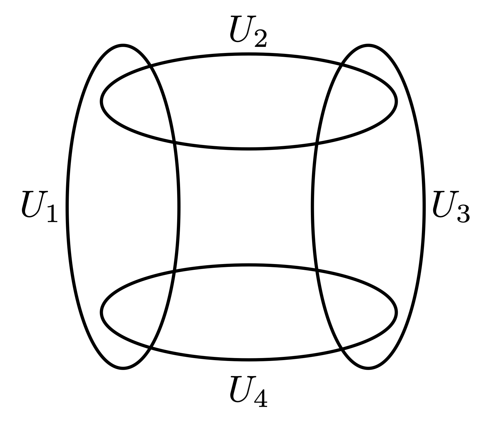
While non-graded Betti numbers can often distinguish ideals from each other, they are insufficient to even detect whether a code is inductively pierced. Consider the polarized neural ideal J1=(x1​x3,x2​x4)J_{1}=(x_{1}x_{3},x_{2}x_{4}). This has the same Betti numbers as J2=(x1​x4,x3​x4)J_{2}=(x_{1}x_{4},x_{3}x_{4}), but only the latter is inductively pierced (see Figure 4.0.1). Here the two neural codes can be distinguished by their graded Betti numbers, or by their regularity (3 for the first ideal, 2 for the second). This incentivizes us to consider graded Betti numbers rather than only non-graded Betti numbers in order to detect inductively pierced codes.

In this paper we go further and consider multi-graded Betti numbers under the multi-grading where deg⁡(xi)=(1,0)\deg(x_{i})=(1,0) and deg⁡(yi)=(0,1)\deg(y_{i})=(0,1). This allows us to differentiate between firing fields that do not intersect and firing fields where one is contained in the other. For example, J3=(x1​x4,x4​y3)J_{3}=(x_{1}x_{4},x_{4}y_{3}) has the same graded Betti numbers as J2J_{2} above. However, for J2J_{2}, U3∩U4=∅U_{3}\cap U_{4}=\emptyset, whereas for J3J_{3}, U4⊆U3U_{4}\subseteq U_{3} (see Figure 4.0.1). Indeed, their multigraded Betti numbers are distinct.
Refer to caption
Refer to caption
Refer to caption
Figure 4.0.1. Realizations of the codes associated to J1J_{1} (top), J2J_{2} (lower left), J3J_{3} (lower right) from Example 4.2.
Definition 4.3.

Let CC be an inductively pierced neural code on nn neurons. Given a piercing order of CC, we define jkj_{k} to be the number of kk-piercings in the piercing order, i.e. with rank​[σ,τ]=k\text{rank}[\sigma,\tau]=k.

We further define jk,vj_{k,v} to be the number of kk-piercings contained in vv other place fields in the piercing order, i.e. with |σ|=v|\sigma|=v and rank​[σ,τ]=k\text{rank}[\sigma,\tau]=k in the notation of Definition 2.20.

Lemma 4.4.

Let CC be an inductively pierced neural code on nn neurons. For 0≤k<n0\leq k<n, we have

jk=∑v=0n−1jk,v=∑v=0n−k−1jk,v.j_{k}=\sum_{v=0}^{n-1}j_{k,v}=\sum_{v=0}^{n-k-1}j_{k,v}.

In particular, a kk-piercing can be contained in at most n−k−1n-k-1 place fields. Moreover, we have

n=∑k=0n−1jk.n=\sum_{k=0}^{n-1}j_{k}.
Proof.

Since we have nn neurons, the first equality follows from that fact that any given place field is contained in no more than n−1n-1 other place fields.

To get the second equality, consider kk and vv such that jk,v≠0j_{k,v}\neq 0. This means there exists at least one UiU_{i} creating a kk-piercing contained in vv other placefields. For this to be possible, we must have

1+k+v≤n.1+k+v\leq n.

As a result, if v>n−1−kv>n-1-k, then jk,v=0j_{k,v}=0, which then gives the second equality.

Lastly, the final summation follows from the fact that every neuron is a piercing and the largest possible piercing with nn neurons is an n−1n-1-piercing. ∎

Example 4.5.

Continuing Example 2.22, we have:

j0,0=1j1,0=2j1,1=1j2,0=1.j_{0,0}=1\quad j_{1,0}=2\quad j_{1,1}=1\quad j_{2,0}=1.

Or we could write

j0=1j1=3j2=1.j_{0}=1\quad j_{1}=3\quad j_{2}=1.
Remark 4.6.

Although inductively pierced codes may have many possible piercing orders, we will show that the numbers jk,vj_{k,v} are independent of the particular order chosen (see Theorem 4.12). This will also have interesting consequences for chordal graphs, see Section 5.

Remark 4.7.

As noted earlier, in order to have a kk-piercing, a neural code must have a (k−1)(k-1)-piercing. As a result, given a piercing order, if jk=0j_{k}=0 for some kk, then ju=0j_{u}=0 for all u>ku>k and CC is at most (k−1)(k-1)-inductively pierced. Similarly, if jk,v=0j_{k,v}=0 for some kk, then ju,v=0j_{u,v}=0 for all u>ku>k.

From Theorem 3.18, we can compute the Betti numbers of an inductively pierced code.

Notation 4.8.

In what follows, δa,b\delta_{a,b} will denote the Kronecker delta function, i.e.

δa,b={1if ​a=b,0else.\delta_{a,b}=\begin{cases}1&\text{if }a=b,\\ 0&\text{else.}\\ \end{cases}
Theorem 4.9.

Suppose 𝒞\mathcal{C} is an inductively pierced neural code on nn neurons, and Jn⊂SJ_{n}\subset S is the polarized neural ideal of 𝒞\mathcal{C}. Given a piercing order of 𝒞\mathcal{C} and corresponding jk,ℓj_{k,\ell}, if w>0w>0 then

βw,w+1−v,vS​(S/Jn)=∑k=0n−1∑ℓ=0n−1(jk,ℓ−δℓ,0)​(n−1−k−ℓw−v)​(ℓv).\beta_{w,w+1-v,v}^{S}\!\left(S/J_{n}\right)=\sum_{k=0}^{n-1}\sum_{\ell=0}^{n-1}\left(j_{k,\ell}-\delta_{\ell,0}\right)\binom{n-1-k-\ell}{w-v}\binom{\ell}{v}.

Moreover, β0,0,0S​(S/Jn)=1\beta_{0,0,0}^{S}\!\left(S/J_{n}\right)=1, and all other Betti numbers are 0.

Proof.

We proceed by induction on nn. For the case of n=1n=1, we have J=(0)J=(0) and so S/J=SS/J=S. Thus,

βw,u,vS​(S/J)={1w=u=v=00 otherwise.\beta_{w,u,v}^{S}\!\left(S/J\right)=\begin{cases}1&w=u=v=0\\ 0&\text{ otherwise}\end{cases}.

For the case of w>0w>0, we note that k=ℓ=0=n−1k=\ell=0=n-1, so jk,ℓ−δℓ,0=0j_{k,\ell}-\delta_{\ell,0}=0, causing the theorized formula for βw,w+1−v,vS​(S/J)\beta_{w,w+1-v,v}^{S}\!\left(S/J\right) also to vanish.

Now suppose the formula holds for some n−1n-1 with n>0n>0 and consider nn such that nn is a kk-piercing contained in ℓ\ell other place fields. Let JnJ_{n} denote the polarized neural ideal for 𝒞\mathcal{C} and Jn−1J_{n-1} the polarized neural ideal for 𝒞\{n}\mathcal{C}\backslash\{n\}. By Theorem 3.18, we have the desired vanishing and β0,0,0S​(S/Jn)=1\beta_{0,0,0}^{S}\!\left(S/J_{n}\right)=1. Thus, we turn our attention to the case of w>0w>0.

If w=1w=1 and u+v=w+1u+v=w+1, then either v=0v=0 or v=1v=1. In the case of v=0v=0, Theorem 3.18 and our induction hypothesis yield

β1,2,0S​(SJn)\displaystyle\beta_{1,2,0}^{S}\!\left(\frac{S}{J_{n}}\right) =(n−1−k−ℓ1)​(ℓ0)+β1,2,0S​(SJn−1)\displaystyle=\tbinom{n-1-k-\ell}{1}\tbinom{\ell}{0}+\beta_{1,2,0}^{S}\!\left(\frac{S}{J_{n-1}}\right)
=(n−1−k−ℓ1)+∑a=0n−2∑b=0n−2(ja,b′−δb,0)​(n−2−a−b1)​(b0)\displaystyle=\tbinom{n-1-k-\ell}{1}+\sum_{a=0}^{n-2}\sum_{b=0}^{n-2}\left(j_{a,b}^{\prime}-\delta_{b,0}\right)\tbinom{n-2-a-b}{1}\tbinom{b}{0}
=(n−1−k−ℓ1)+∑a=0n−2∑b=0n−2(ja,b′−δb,0)​(n−2−a−b1)\displaystyle=\tbinom{n-1-k-\ell}{1}+\sum_{a=0}^{n-2}\sum_{b=0}^{n-2}\left(j_{a,b}^{\prime}-\delta_{b,0}\right)\tbinom{n-2-a-b}{1}
=(n−1−k−ℓ1)+∑a=0n−2∑b=0n−2(ja,b′−δb,0)​[(n−1−a−b1)−(n−2−a−b0)]\displaystyle=\tbinom{n-1-k-\ell}{1}+\sum_{a=0}^{n-2}\sum_{b=0}^{n-2}\left(j_{a,b}^{\prime}-\delta_{b,0}\right)\left[\tbinom{n-1-a-b}{1}-\tbinom{n-2-a-b}{0}\right]
=(n−1−k−ℓ1)+∑a=0n−2∑b=0n−2(ja,b′−δb,0)​(n−1−a−b1)−∑a=0n−2∑b=0n−2(ja,b′−δb,0)\displaystyle=\tbinom{n-1-k-\ell}{1}+\sum_{a=0}^{n-2}\sum_{b=0}^{n-2}\left(j_{a,b}^{\prime}-\delta_{b,0}\right)\tbinom{n-1-a-b}{1}-\sum_{a=0}^{n-2}\sum_{b=0}^{n-2}\left(j_{a,b}^{\prime}-\delta_{b,0}\right)
=(n−1−k−ℓ1)+∑a=0n−2∑b=0n−2(ja,b′−δb,0)​(n−1−a−b1)−∑a=0n−2(ja−1)⏟=0\displaystyle=\tbinom{n-1-k-\ell}{1}+\sum_{a=0}^{n-2}\sum_{b=0}^{n-2}\left(j_{a,b}^{\prime}-\delta_{b,0}\right)\tbinom{n-1-a-b}{1}-\underset{=0}{\underbrace{\sum_{a=0}^{n-2}\left(j_{a}-1\right)}}
=(n−1−k−ℓ1)+∑a=0n−2∑b=0n−2(ja,b′−δb,0)​(n−1−a−b1)\displaystyle=\tbinom{n-1-k-\ell}{1}+\sum_{a=0}^{n-2}\sum_{b=0}^{n-2}\left(j_{a,b}^{\prime}-\delta_{b,0}\right)\tbinom{n-1-a-b}{1}

If nn is contained in all other place fields, then ℓ=n−1\ell=n-1 and nn must be a 0-piercing, so k=0k=0. This yields (n−1−k−ℓ1)=(01)=0\tbinom{n-1-k-\ell}{1}=\tbinom{0}{1}=0 and so

β1,2,0S​(SJn)=∑a=0n−2∑b=0n−2(ja,b′−δb,0)​(n−1−a−b1).\beta_{1,2,0}^{S}\!\left(\frac{S}{J_{n}}\right)=\sum_{a=0}^{n-2}\sum_{b=0}^{n-2}\left(j_{a,b}^{\prime}-\delta_{b,0}\right)\tbinom{n-1-a-b}{1}.

Now noting that if either a=n−1a=n-1 or b=n−1b=n-1, then (n−1−a−b1)=0\tbinom{n-1-a-b}{1}=0 and thus it must be vacuously true that

β1,2,0S​(SJn)\displaystyle\beta_{1,2,0}^{S}\!\left(\frac{S}{J_{n}}\right) =∑a=0n−1∑b=0n−1(ja,b′−δb,0)​(n−1−a−b1)\displaystyle=\sum_{a=0}^{n-1}\sum_{b=0}^{n-1}\left(j_{a,b}^{\prime}-\delta_{b,0}\right)\tbinom{n-1-a-b}{1}
=∑a=0n−1∑b=0n−1(ja,b′−δb,0)​(n−1−a−b1)​(b0)\displaystyle=\sum_{a=0}^{n-1}\sum_{b=0}^{n-1}\left(j_{a,b}^{\prime}-\delta_{b,0}\right)\tbinom{n-1-a-b}{1}\tbinom{b}{0}
=∑a=0n−1∑b=0n−1(ja,b−δb,0)​(n−1−a−b1)​(b0).\displaystyle=\sum_{a=0}^{n-1}\sum_{b=0}^{n-1}\left(j_{a,b}-\delta_{b,0}\right)\tbinom{n-1-a-b}{1}\tbinom{b}{0}.

Using the same arguments, the case of w=u=v=1w=u=v=1 yields

β1,1,1S​(SJn)\displaystyle\beta_{1,1,1}^{S}\!\left(\frac{S}{J_{n}}\right) =(ℓ1)+∑a=0n−2∑b=0n−2(ja,b′−δb,0)​(b1)\displaystyle=\tbinom{\ell}{1}+\sum_{a=0}^{n-2}\sum_{b=0}^{n-2}\left(j_{a,b}^{\prime}-\delta_{b,0}\right)\tbinom{b}{1}
=(ℓ1)+∑a=0n−2∑b=0n−2(ja,b′−δb,0)​b\displaystyle=\tbinom{\ell}{1}+\sum_{a=0}^{n-2}\sum_{b=0}^{n-2}\left(j_{a,b}^{\prime}-\delta_{b,0}\right)b
=(ℓ1)+∑a=0n−2∑b=0n−2b​ja,b′−∑a=0n−2∑b=0n−2b​δb,0⏟=0\displaystyle=\tbinom{\ell}{1}+\sum_{a=0}^{n-2}\sum_{b=0}^{n-2}bj_{a,b}^{\prime}-\sum_{a=0}^{n-2}\sum_{b=0}^{n-2}\underset{=0}{\underbrace{b\delta_{b,0}}}
=(ℓ1)+∑a=0n−2∑b=0n−2b​ja,b′.\displaystyle=\tbinom{\ell}{1}+\sum_{a=0}^{n-2}\sum_{b=0}^{n-2}bj_{a,b}^{\prime}.

Now, if 0≤k≤n−20\leq k\leq n-2 and 0≤ℓ≤n−20\leq\ell\leq n-2, then we set

ja,b={ja,b′+1k=a​ and ​ℓ=bja,b′otherwise.j_{a,b}=\begin{cases}j_{a,b}^{\prime}+1&k=a\text{ and }\ell=b\\ j_{a,b}^{\prime}&\text{otherwise}\end{cases}.

We further extend this by setting ja,b=0j_{a,b}=0 is a=n−1a=n-1 or b=n−1b=n-1, which produces

β1,1,1S​(SJn)\displaystyle\beta_{1,1,1}^{S}\!\left(\frac{S}{J_{n}}\right) =∑a=0n−1∑b=0n−1b​ja,b\displaystyle=\sum_{a=0}^{n-1}\sum_{b=0}^{n-1}bj_{a,b}
=∑a=0n−1∑b=0n−1(ja,b−δb,0)​(n−1−a−b0)​(b1).\displaystyle=\sum_{a=0}^{n-1}\sum_{b=0}^{n-1}\left(j_{a,b}-\delta_{b,0}\right)\tbinom{n-1-a-b}{0}\tbinom{b}{1}.

If k=n−1k=n-1 or ℓ=n−1\ell=n-1, then we set

ja,b={1k=a​ and ​ℓ=bja,b′a,b<n−10otherwise.j_{a,b}=\begin{cases}1&k=a\text{ and }\ell=b\\ j_{a,b}^{\prime}&a,b<n-1\\ 0&\text{otherwise}\end{cases}.

The result follows as in the previous case.

We finally turn our attention to the simpler case of w>1w>1. From the induction hypothesis, we observe that

βw−1,w−v,vS​(SJn−1)+βw,w+1−v,vS​(SJn−1)\displaystyle\beta_{w-1,w-v,v}^{S}\!\left(\frac{S}{J_{n-1}}\right)+\beta_{w,w+1-v,v}^{S}\!\left(\frac{S}{J_{n-1}}\right)\hskip-142.26378pt
=\displaystyle= ∑a=0n−2∑b=0n−2(ja,b′−δb,0)​(n−2−a−bw−1−v)​(bv)+∑a=0n−2∑b=0n−2(ja,b′−δb,0)​(n−2−a−bw−v)​(bv)\displaystyle\sum_{a=0}^{n-2}\sum_{b=0}^{n-2}\left(j_{a,b}^{\prime}-\delta_{b,0}\right)\tbinom{n-2-a-b}{w-1-v}\tbinom{b}{v}+\sum_{a=0}^{n-2}\sum_{b=0}^{n-2}\left(j_{a,b}^{\prime}-\delta_{b,0}\right)\tbinom{n-2-a-b}{w-v}\tbinom{b}{v}
=\displaystyle= ∑a=0n−2∑b=0n−2(ja,b′−δb,0)​[(n−2−a−bw−1−v)+(n−2−a−bw−v)]​(bv)\displaystyle\sum_{a=0}^{n-2}\sum_{b=0}^{n-2}\left(j_{a,b}^{\prime}-\delta_{b,0}\right)\left[\tbinom{n-2-a-b}{w-1-v}+\tbinom{n-2-a-b}{w-v}\right]\tbinom{b}{v}
=\displaystyle= ∑a=0n−2∑b=0n−2(ja,b′−δb,0)​(n−1−a−bw−v)​(bv).\displaystyle\sum_{a=0}^{n-2}\sum_{b=0}^{n-2}\left(j_{a,b}^{\prime}-\delta_{b,0}\right)\tbinom{n-1-a-b}{w-v}\tbinom{b}{v}.

Combining this with Theorem 3.18 then gives

βw,w+1−v,vS​(SJn)\displaystyle\beta_{w,w+1-v,v}^{S}\!\left(\frac{S}{J_{n}}\right) =(n−1−k−ℓw−v)​(ℓv)+βw−1,w−v,vS​(SJn−1)+βw,w+1−v,vS​(SJn−1)\displaystyle=\tbinom{n-1-k-\ell}{w-v}\tbinom{\ell}{v}+\beta_{w-1,w-v,v}^{S}\!\left(\frac{S}{J_{n-1}}\right)+\beta_{w,w+1-v,v}^{S}\!\left(\frac{S}{J_{n-1}}\right)
=(n−1−k−ℓw−v)​(ℓv)+∑a=0n−2∑b=0n−2(ja,b′−δb,0)​(n−1−a−bw−v)​(bv).\displaystyle=\tbinom{n-1-k-\ell}{w-v}\tbinom{\ell}{v}+\sum_{a=0}^{n-2}\sum_{b=0}^{n-2}\left(j_{a,b}^{\prime}-\delta_{b,0}\right)\tbinom{n-1-a-b}{w-v}\tbinom{b}{v}.

From here, the same reasoning used in the case of w=1w=1 to relate ja,bj_{a,b} and ja,b′j_{a,b}^{\prime} applies and gives the desired result. ∎

Similar formulas arise for Betti numbers and graded Betti numbers.

Corollary 4.10.

Given the same setup as in Theorem 4.9, the graded Betti numbers of 𝒞\mathcal{C} are given by:

βw,iS​(S/J)={1w=i=0∑k=0n−1(jk−1)​(n−1−kw)i=w+1≥20otherwise.\beta_{w,i}^{S}\!\left(S/J\right)=\begin{cases}1&w=i=0\\ \sum_{k=0}^{n-1}(j_{k}-1)\binom{n-1-k}{w}&i=w+1\geq 2\\ 0&\text{otherwise}\end{cases}.

The total Betti numbers of 𝒞\mathcal{C} are given by:

βwS​(S/J)={1w=0∑k=0n−1(jk−1)​(n−1−kw)w>0.\beta_{w}^{S}\!\left(S/J\right)=\begin{cases}1&w=0\\ \sum_{k=0}^{n-1}(j_{k}-1)\binom{n-1-k}{w}&w>0\end{cases}.
Proof.

These formulas can be obtained using the same method as Theorem 4.9 but using Corollary 3.19 and Corollary 3.20, respectively, in place of Theorem 3.18. Alternatively, these results can be found by combining Theorem 4.9 with

βw,iS​(S/J)=∑u+v=iβw,u,vS​(S/J)\beta_{w,i}^{S}\!\left(S/J\right)=\sum_{u+v=i}\beta_{w,u,v}^{S}\!\left(S/J\right)

and applying combinatorial identities. ∎

The relationship between the Betti numbers and the piercing numbers can be expressed in a linear equation.

Corollary 4.11.

Writing βw,i=βw,iS​(S/J)\beta_{w,i}=\beta_{w,i}^{S}\!\left(S/J\right), Corollary 4.10 can be summarized in the following equation.

(βn−1,nβn−2,n−1⋮β2,3β1,2β0,1)⏟β→+1​(S/J)\displaystyle\underset{\vec{\beta}_{+1}(S/J)}{\underbrace{\begin{pmatrix}\beta_{n-1,n}\\ \beta_{n-2,n-1}\\ \vdots\\ \beta_{2,3}\\ \beta_{1,2}\\ \beta_{0,1}\end{pmatrix}}} =((n−1n−1)0⋯000(n−1n−2)(n−2n−2)000⋮⋮⋱⋮⋮(n−12)(n−22)⋯(22)00(n−11)(n−21)⋯(21)(11)0(n−10)(n−20)⋯(20)(10)(00))⏟An​(j0−1j1−1⋮jn−3−1jn−2−1jn−1−1)⏟j→​(S/J)−1\displaystyle=\underset{A_{n}}{\underbrace{\begin{pmatrix}\tbinom{n-1}{n-1}&0&\cdots&0&0&0\\ \tbinom{n-1}{n-2}&\tbinom{n-2}{n-2}&&0&0&0\\ \vdots&\vdots&\ddots&&\vdots&\vdots\\ \tbinom{n-1}{2}&\tbinom{n-2}{2}&\cdots&\tbinom{2}{2}&0&0\\ \tbinom{n-1}{1}&\tbinom{n-2}{1}&\cdots&\tbinom{2}{1}&\tbinom{1}{1}&0\\ \tbinom{n-1}{0}&\tbinom{n-2}{0}&\cdots&\tbinom{2}{0}&\tbinom{1}{0}&\binom{0}{0}\end{pmatrix}}}\underset{\vec{j}(S/J)-\textbf{1}}{\underbrace{\begin{pmatrix}j_{0}-1\\ j_{1}-1\\ \vdots\\ j_{n-3}-1\\ j_{n-2}-1\\ j_{n-1}-1\end{pmatrix}}}

Moreover, the matrix AnA_{n} is an invertible matrix and thus the Betti numbers and piercing numbers are in a one-to-one correspondence. Therefore, the piercing numbers are independent of the piercing order and are given by

jk=1+∑w=n−1−kn−1(wn−1−k)​(−1)w−n+1+k​βw,w+1S​(S/J).j_{k}=1+\sum_{w=n-1-k}^{n-1}\binom{w}{n-1-k}(-1)^{w-n+1+k}\beta_{w,w+1}^{S}\!\left(S/J\right).
Proof.

The equation follows from Corollary 4.10. The matrix AnA_{n} is a lower triangular matrix whose main diagonal consists of only ones, thus AnA_{n} is invertible. This puts the Betti numbers and piercing numbers into a one-to-one correspondence. That is, we have

j→​(S/J)−1=An−1⋅β→+1​(S/J).\vec{j}(S/J)-\textbf{1}=A_{n}^{-1}\cdot\vec{\beta}_{+1}(S/J).

Since the Betti numbers are independent of the piercing order, the piercing numbers must also be independent of the piercing order.

Moreover, the matrix AnA_{n} is sometimes referred to as the Pascal Matrix whose inverse is given by

An−1=((n−1n−1)0⋯000−(n−1n−2)(n−2n−2)000⋮⋮⋱⋮⋮(−1)n−1​(n−12)(−1)n​(n−22)⋯(22)00(−1)n​(n−11)(−1)n+1​(n−21)⋯−(21)(11)0(−1)n+1​(n−10)(−1)n+2​(n−20)⋯(20)−(10)(00)).A_{n}^{-1}=\left(\begin{smallmatrix}\tbinom{n-1}{n-1}&0&\cdots&0&0&0\\ -\tbinom{n-1}{n-2}&\tbinom{n-2}{n-2}&&0&0&0\\ \vdots&\vdots&\ddots&&\vdots&\vdots\\ (-1)^{n-1}\tbinom{n-1}{2}&(-1)^{n}\tbinom{n-2}{2}&\cdots&\tbinom{2}{2}&0&0\\ (-1)^{n}\tbinom{n-1}{1}&(-1)^{n+1}\tbinom{n-2}{1}&\cdots&-\tbinom{2}{1}&\tbinom{1}{1}&0\\ (-1)^{n+1}\tbinom{n-1}{0}&(-1)^{n+2}\tbinom{n-2}{0}&\cdots&\tbinom{2}{0}&-\tbinom{1}{0}&\binom{0}{0}\end{smallmatrix}\right).

The formula for jkj_{k} follows by inputting the above matrix into the linear equation j→​(S/J)−1=An−1⋅β→+1​(S/J)\vec{j}(S/J)-\textbf{1}=A_{n}^{-1}\cdot\vec{\beta}_{+1}(S/J). ∎

A similar result holds for jk,ℓj_{k,\ell}, however the linear algebra approach is not quite as clean as the above proof. Instead, we obtain the following result using combinatorial formulas.

Theorem 4.12.

Let 𝒞\mathcal{C} be an inductively pierced neural code on nn neurons, and JJ the polarized neural ideal of 𝒞\mathcal{C} in the ring SS. Given a piercing order, let ja,bj_{a,b} denote the number of aa-piercings of 𝒞\mathcal{C} contained in exactly bb other place fields. Then

ja,b=δb,0+∑v=0n−1∑w=0n−1βw,w+1−v,vS​(S/J)​(w−vn−1−a−b)​(vb)​(−1)w−n+1+a.j_{a,b}=\delta_{b,0}+\sum_{v=0}^{n-1}\sum_{w=0}^{n-1}\beta_{w,w+1-v,v}^{S}\!\left(S/J\right)\binom{w-v}{n-1-a-b}\binom{v}{b}(-1)^{w-n+1+a}.

As a consequence, the ja,bj_{a,b} are independent of the choice of piercing order.

Remark 4.13.

This corollary implies that the results of this section do not depend on the choice of piercing order.

Proof.

For brevity, set αk,ℓ=jk,ℓ−δℓ,0\alpha_{k,\ell}=j_{k,\ell}-\delta_{\ell,0}.

∑v=0n−1∑w=0n−1βw,w+1−v,vS​(SJ)​(w−vn−1−a−b)​(vb)​(−1)w−n+1+a\displaystyle\sum_{v=0}^{n-1}\sum_{w=0}^{n-1}\beta_{w,w+1-v,v}^{S}\!\left(\frac{S}{J}\right)\tbinom{w-v}{n-1-a-b}\tbinom{v}{b}(-1)^{w-n+1+a}\hskip-99.58464pt
=\displaystyle= ∑v=0n−1∑u=−vn−1−vβu+v,u+1,vS​(SJ)​(un−1−a−b)​(vb)​(−1)u+v−n+1+a\displaystyle\sum_{v=0}^{n-1}\sum_{u=-v}^{n-1-v}\beta_{u+v,u+1,v}^{S}\!\left(\frac{S}{J}\right)\tbinom{u}{n-1-a-b}\tbinom{v}{b}(-1)^{u+v-n+1+a}

We note that if v>0v>0, then whenever −v≤u<0-v\leq u<0, we have (un−1−a−b)=0\tbinom{u}{n-1-a-b}=0. Thus, we can change the lower bound of the inner sum from u=−vu=-v to u=0u=0 to get

∑v=0n−1∑u=0n−1−vβu+v,u+1,vS​(SJ)​(un−1−a−b)​(vb)​(−1)u+v−n+1+a.\sum_{v=0}^{n-1}\sum_{u=0}^{n-1-v}\beta_{u+v,u+1,v}^{S}\!\left(\frac{S}{J}\right)\tbinom{u}{n-1-a-b}\tbinom{v}{b}(-1)^{u+v-n+1+a}.

Next, if u>n−1−vu>n-1-v, then w=u+v>n−1w=u+v>n-1 which implies βw,u,vS​(S/J)=0\beta_{w,u,v}^{S}\!\left(S/J\right)=0 since the projective dimension of S/JS/J is, at most, n−1n-1. As such the upper bound of the inner sum can be changed from u=n−1−vu=n-1-v to u=n−1u=n-1. With this we obtain the following.

∑v=0n−1∑w=0n−1βw,w+1−v,vS​(SJ)​(w−vn−1−a−b)​(vb)​(−1)w−n+1+a\displaystyle\sum_{v=0}^{n-1}\sum_{w=0}^{n-1}\beta_{w,w+1-v,v}^{S}\!\left(\frac{S}{J}\right)\tbinom{w-v}{n-1-a-b}\tbinom{v}{b}(-1)^{w-n+1+a}\hskip-142.26378pt
=\displaystyle= ∑v=0n−1∑u=0n−1βu+v,u+1,vS​(SJ)​(un−1−a−b)​(vb)​(−1)u+v−n+1+a\displaystyle\sum_{v=0}^{n-1}\sum_{u=0}^{n-1}\beta_{u+v,u+1,v}^{S}\!\left(\frac{S}{J}\right)\tbinom{u}{n-1-a-b}\tbinom{v}{b}(-1)^{u+v-n+1+a}
=\displaystyle= ∑v=0n−1∑u=0n−1∑k=0n−1∑ℓ=0n−1αk,ℓ​(n−1−k−ℓu)​(ℓv)​(un−1−a−b)​(vb)​(−1)u+v−n+1+a\displaystyle\sum_{v=0}^{n-1}\sum_{u=0}^{n-1}\sum_{k=0}^{n-1}\sum_{\ell=0}^{n-1}\alpha_{k,\ell}\tbinom{n-1-k-\ell}{u}\tbinom{\ell}{v}\tbinom{u}{n-1-a-b}\tbinom{v}{b}(-1)^{u+v-n+1+a}
=\displaystyle= ∑k=0n−1∑ℓ=0n−1αk,ℓ​∑v=0n−1∑u=0n−1(ℓv)​(vb)​(n−1−k−ℓu)​(un−1−a−b)​(−1)u+v−n+1+a\displaystyle\sum_{k=0}^{n-1}\sum_{\ell=0}^{n-1}\alpha_{k,\ell}\sum_{v=0}^{n-1}\sum_{u=0}^{n-1}\tbinom{\ell}{v}\tbinom{v}{b}\tbinom{n-1-k-\ell}{u}\tbinom{u}{n-1-a-b}(-1)^{u+v-n+1+a}

Next, we use Example B.2(6) to get (ℓv)​(vb)=(ℓb)​(ℓ−bv−b)\tbinom{\ell}{v}\tbinom{v}{b}=\tbinom{\ell}{b}\tbinom{\ell-b}{v-b}. With this equality, we find

∑v=0n−1∑w=0n−1βw,w+1−v,vS​(SJ)​(w−vn−1−a−b)​(vb)​(−1)w−n+1+a\displaystyle\sum_{v=0}^{n-1}\sum_{w=0}^{n-1}\beta_{w,w+1-v,v}^{S}\!\left(\frac{S}{J}\right)\tbinom{w-v}{n-1-a-b}\tbinom{v}{b}(-1)^{w-n+1+a}\hskip-170.71652pt
=\displaystyle= ∑k=0n−1∑ℓ=0n−1αk,ℓ​∑v=0n−1∑u=0n−1(ℓb)​(ℓ−bv−b)​(n−1−k−ℓu)​(un−1−a−b)​(−1)u+v−n+1+a\displaystyle\sum_{k=0}^{n-1}\sum_{\ell=0}^{n-1}\alpha_{k,\ell}\sum_{v=0}^{n-1}\sum_{u=0}^{n-1}\tbinom{\ell}{b}\tbinom{\ell-b}{v-b}\tbinom{n-1-k-\ell}{u}\tbinom{u}{n-1-a-b}(-1)^{u+v-n+1+a}
=\displaystyle= ∑k=0n−1∑ℓ=0n−1αk,ℓ​∑u=0n−1∑v=0n−1(ℓb)​(ℓ−bv−b)​(n−1−k−ℓu)​(un−1−a−b)​(−1)u+v−n+1+a\displaystyle\sum_{k=0}^{n-1}\sum_{\ell=0}^{n-1}\alpha_{k,\ell}\sum_{u=0}^{n-1}\sum_{v=0}^{n-1}\tbinom{\ell}{b}\tbinom{\ell-b}{v-b}\tbinom{n-1-k-\ell}{u}\tbinom{u}{n-1-a-b}(-1)^{u+v-n+1+a}
=\displaystyle= ∑k=0n−1∑ℓ=0n−1αk,ℓ​(ℓb)​∑u=0n−1(n−1−k−ℓu)​(un−1−a−b)​(−1)u+b−n+1+a​∑v=0n−1(ℓ−bv−b)​(−1)v−b\displaystyle\sum_{k=0}^{n-1}\sum_{\ell=0}^{n-1}\alpha_{k,\ell}\tbinom{\ell}{b}\sum_{u=0}^{n-1}\tbinom{n-1-k-\ell}{u}\tbinom{u}{n-1-a-b}(-1)^{u+b-n+1+a}\sum_{v=0}^{n-1}\tbinom{\ell-b}{v-b}(-1)^{v-b}
=\displaystyle= ∑k=0n−1αk,b​(bb)​∑u=0n−1(n−1−k−bu)​(un−1−a−b)​(−1)u+b−n+1+a\displaystyle\sum_{k=0}^{n-1}\alpha_{k,b}\tbinom{b}{b}\sum_{u=0}^{n-1}\tbinom{n-1-k-b}{u}\tbinom{u}{n-1-a-b}(-1)^{u+b-n+1+a}

where the last equality follows from Example B.2(4) gives

∑v=0n−1(ℓ−bv−b)​(−1)v−b=∑v=bℓ(ℓ−bv−b)​(−1)v−b=∑v=0ℓ−b(ℓ−bv)​(−1)v={1ℓ=b0ℓ≠b.\sum_{v=0}^{n-1}\tbinom{\ell-b}{v-b}(-1)^{v-b}=\sum_{v=b}^{\ell}\tbinom{\ell-b}{v-b}(-1)^{v-b}=\sum_{v=0}^{\ell-b}\tbinom{\ell-b}{v}(-1)^{v}=\begin{cases}1&\ell=b\\ 0&\ell\neq b\end{cases}.

By similar reasoning, we get (n−1−k−bu)​(un−1−a−b)=(n−1−k−bn−1−a−b)​(a−ku−n+1+a+b)\tbinom{n-1-k-b}{u}\tbinom{u}{n-1-a-b}=\tbinom{n-1-k-b}{n-1-a-b}\tbinom{a-k}{u-n+1+a+b} and

∑u=0n−1(a−ku−n+1+a+b)​(−1)u−n+1+a+b={1k=a0k≠a.\sum_{u=0}^{n-1}\tbinom{a-k}{u-n+1+a+b}(-1)^{u-n+1+a+b}=\begin{cases}1&k=a\\ 0&k\neq a\end{cases}.

This allows for the following computation.

∑v=0n−1∑w=0n−1βw,w+1−v,vS​(SJ)​(w−vn−1−a−b)​(vb)​(−1)w−n+1+a\displaystyle\sum_{v=0}^{n-1}\sum_{w=0}^{n-1}\beta_{w,w+1-v,v}^{S}\!\left(\frac{S}{J}\right)\tbinom{w-v}{n-1-a-b}\tbinom{v}{b}(-1)^{w-n+1+a}\hskip-99.58464pt
=\displaystyle= ∑k=0n−1αk,b​(bb)​∑u=0n−1(n−1−k−bn−1−a−b)​(a−ku−n+1+a+b)​(−1)u+b−n+1+a\displaystyle\sum_{k=0}^{n-1}\alpha_{k,b}\tbinom{b}{b}\sum_{u=0}^{n-1}\tbinom{n-1-k-b}{n-1-a-b}\tbinom{a-k}{u-n+1+a+b}(-1)^{u+b-n+1+a}
=\displaystyle= ∑k=0n−1αk,b​(bb)​(n−1−k−bn−1−a−b)​∑u=0n−1(a−ku−n+1+a+b)​(−1)u+b−n+1+a\displaystyle\sum_{k=0}^{n-1}\alpha_{k,b}\tbinom{b}{b}\tbinom{n-1-k-b}{n-1-a-b}\sum_{u=0}^{n-1}\tbinom{a-k}{u-n+1+a+b}(-1)^{u+b-n+1+a}
=\displaystyle= αa,b​(bb)​(n−1−a−bn−1−a−b)\displaystyle\alpha_{a,b}\tbinom{b}{b}\tbinom{n-1-a-b}{n-1-a-b}
=\displaystyle= αa,b\displaystyle\alpha_{a,b}
=\displaystyle= ja,b−δb,0.\displaystyle j_{a,b}-\delta_{b,0}.

Adding δb,0\delta_{b,0} to both sides provides the result. ∎

Next we compute the projective dimensions of inductively pierced codes.

Corollary 4.14.

Let 𝒞\mathcal{C} be a kk-inductively pierced neural code on nn neurons, and JJ the polarized neural ideal of 𝒞\mathcal{C} in the ring SS.

Given a piercing order, if j0=⋯=jt−1=1j_{0}=\cdots=j_{t-1}=1 for some t>0t>0, then βn−u−1S​(S/J)=0\beta_{n-u-1}^{S}\!\left(S/J\right)=0 for 0≤u<t0\leq u<t.

Moreover, if t≥0t\geq 0 is the smallest integer such that jt>1j_{t}>1, then pdS⁡S/J=n−1−t\operatorname{pd}_{S}S/J=n-1-t.

Proof.

We start by assuming j0=⋯=jt−1=1j_{0}=\cdots=j_{t-1}=1 for some t>0t>0 and let 0≤u<t0\leq u<t. We then find the following:

βn−u−1S​(S/J)\displaystyle\beta_{n-u-1}^{S}\!\left(S/J\right) =∑k=0n−1(jk−1)​(n−1−kn−1−u)\displaystyle=\sum_{k=0}^{n-1}\left(j_{k}-1\right)\binom{n-1-k}{n-1-u}
=∑k=tn−1(jk−1)​(n−1−kn−1−u).\displaystyle=\sum_{k=t}^{n-1}\left(j_{k}-1\right)\binom{n-1-k}{n-1-u}.

Thus we have u<t≤ku<t\leq k, and so n−1−u>n−1−kn-1-u>n-1-k. This yields (n−1−kn−1−u)=0\tbinom{n-1-k}{n-1-u}=0 for all 0≤u<t0\leq u<t and thus βn−u−1S​(S/J)=0\beta_{n-u-1}^{S}\!\left(S/J\right)=0.

If we further suppose jt>1j_{t}>1, then we obtain

βn−t−1S​(S/J)=∑k=tn−1(jk−1)​(n−1−kn−1−t)=(jt−1)​(n−1−tn−1−t)=jt−1>0.\beta_{n-t-1}^{S}\!\left(S/J\right)=\sum_{k=t}^{n-1}\left(j_{k}-1\right)\binom{n-1-k}{n-1-t}=\left(j_{t}-1\right)\binom{n-1-t}{n-1-t}=j_{t}-1>0.

Since βn−1−tS​(S/J)≠0\beta_{n-1-t}^{S}\!\left(S/J\right)\neq 0 but βn−u−1S​(S/J)=0\beta_{n-u-1}^{S}\!\left(S/J\right)=0 for 0≤u<t0\leq u<t, we must have pdS⁡S/J=n−1−t\operatorname{pd}_{S}S/J=n-1-t. ∎

Remark 4.15.

While the multigraded Betti numbers of an inductively pierced neural code do give substantial information on the piercings, they can’t completely distinguish all features of codes. For example, the following two neural ideals on 5 neurons have the same multigraded Betti numbers:

IA=(x1​x3,x1​x4,x1​x5,x2​x4,x2​x5),\displaystyle I_{A}=(x_{1}x_{3},x_{1}x_{4},x_{1}x_{5},x_{2}x_{4},x_{2}x_{5}),
IB=(x1​x3,x1​x4,x1​x5,x2​x4,x4​x5).\displaystyle I_{B}=(x_{1}x_{3},x_{1}x_{4},x_{1}x_{5},x_{2}x_{4},x_{4}x_{5}).
Refer to caption
Refer to caption
Figure 4.0.2. At left, a realization of the code of ideal IAI_{A}. At right, that of IBI_{B}.

Figure 4.0.2 shows realizations of these two codes. However, a Macaulay2 computation [M2] shows that the toric ideals of the corresponding neural codes (as defined in [GrossObatakeYoungs]) are distinct; in particular the toric ideal of the first example has 15 generators, whereas the toric ideal of the second example has 17 generators. This does hint that the toric ideal of a neural code is a finer invariant than even multigraded Betti numbers. However, current results on toric ideals of neural codes only describe connections to kk-inductively pierced codes for small values of kk [toricideals, toricideals2].

5. A result on chordal graphs

Inductively pierced codes, as previously noted, are closely related to chordal graphs. In this section, we use the connection between the two to show how one of our own results (namely, Corollary 4.11) also proves a theorem about chordal graphs. First, we provide some definitions, and a well-known result, all as in [West].

Definition 5.1.

A graph GG is chordal if it has no chordless cycle (i.e., every cycle of length ≥4\geq 4 has a chord).

One notable property of chordal graphs is that they can be deconstructed by removing so-called simplicial vertices. In fact, this feature characterizes the graph.

Definition 5.2.

A vertex of a graph G=(V,E)G=(V,E) is simplicial if its neighborhood forms a clique. That is, v∈Vv\in V is simplicial if for all vertices u,wu,w so that {v,w}\{v,w\} and {v,u}\{v,u\} form edges, {u,w}\{u,w\} also forms an edge.

Definition 5.3.

A simplicial elimination ordering is an ordering vn,…,v1v_{n},...,v_{1} for deletion of vertices so that each vertex vi+1v_{i+1} is a simplicial vertex of the remaining graph induced by v1,…,viv_{1},...,v_{i}.

Theorem 5.4.

A graph is chordal if and only if it has a simplicial elimination ordering.

In previous work [curry2022recognizing] it has been shown that inductively pierced codes are characterized, in part, by their similarity to chordal graphs. The following definition and theorem are from [curry2022recognizing], but the theorem is provided here (as in Section 2) in its polarized form.

Definition 2.23.

Let 𝒞\mathcal{C} be a code on nn neurons that has a degree two canonical form. The general relationship graph G​(𝒞)G(\mathcal{C}) is the graph with vertices V=[n]V=[n], and an edge i,j{i,j} if and only if the canonical form of JJ does not contain any of the pseudo-monomials xi​xjx_{i}x_{j}, xi​yjx_{i}y_{j}, or xj​yix_{j}y_{i}.

Theorem 2.25.

A neural code 𝒞\mathcal{C} is inductively pierced if and only if

  1. (1)

    C​F​(𝒞)CF(\mathcal{C}) consists entirely of degree two polynomials and

  2. (2)

    the graph G​(𝒞)G(\mathcal{C}) is chordal.

Intuitively, this result holds because the two structures have a major similarity: both can be built up (or taken apart, depending on your point of view) by successively adding (removing) an object that relates to its neighbors at that stage in a very particular way. A piercing order is usually viewed as constructive and so is the reverse of an elimination order, but the concept is the same.

The proof of this characterization (in [curry2022recognizing]) shows that a simplicial elimination ordering on the graph can always be found that reverses to a piercing order; however, all the difficulties of the proof come from the existence of pseudo-monomials of the form xi​yjx_{i}y_{j}, and ensuring that the order is consistent with these. In a code with no yjy_{j} appearing, any simplicial elimination ordering on G​(𝒞)G(\mathcal{C}) reverses to a piercing order. Moreover, the degree kk of the simplicial vertex in the elimination ordering corresponds precisely to the kk of the kk-piercing in the corresponding piercing order.

We also note that every chordal graph is the general relationship graph for a neural code (in fact, usually for many!). Thus, we can use our Corollary 4.11, which implies that the number of kk-piercings in any piercing order is a characteristic of the code, to obtain the following result on chordal graphs.

Theorem 5.5.

Let GG be a chordal graph. The number of vertices of simplicial degree kk removed in any simplicial elimination ordering is fixed.

6. Acknowledgments

The authors would like to thank Michael DeBellevue, Carina Curto, Juliann Geraci, Selvi Kara, and Keri Ann Sather-Wagstaff for helpful conversations throughout the process of writing this paper. The first two authors would also like to thank Justin Roy Cox, Gabriel Lumpkin, Swan Klein, and Connor William Poulton for their work on a semester-long project through the Mason Experimental Geometry Lab, in which they computed the Betti numbers of several families of neural codes. Their work ultimately convinced the authors to look for different classes of neural codes to study, resulting in the research in this paper. During the writing of this paper, the second-named author was partially supported by NSF grant DMS-2424326 and the third-named author by NSF grant DMS–2401482. The last-named author was supported by the Haynesville Project.

This work represents the views of the authors and is not to be regarded as representing the opinions of the Center for Naval Analyses or any of its sponsors.

Appendix A Additional homological background material

In this section we define some of the algebraic terms used in the paper, and give references for the reader to learn more about them.

Much of the material immediately following can be found in [Eisenbud].

Definition A.1.

Let SS be a commutative Noetherian local (resp. graded) ring, k=S/mk=S/m where mm is the (homogeneous) maximal ideal, and MM a finitely generated (graded) SS-module. A free resolution F∙F_{\bullet} of MM is minimal if the differentials of F∙⊗kF_{\bullet}\otimes k are all equal to 0.

Definition A.2.

Let SS be a commutative Noetherian graded ring and MM a finitely generated graded SS-module. Take F∙F_{\bullet} to be a minimal graded free resolution of MM.

  1. (1)

    The Betti numbers of MM are given by

    βi​(M):=rank​(Fi).\beta_{i}(M):=\mathrm{rank}\,(F_{i}).
  2. (2)

    The graded Betti numbers of MM are given by

    βi,j​(M):=rank​(Fi​(−j)).\beta_{i,j}(M):=\mathrm{rank}\,(F_{i}(-j)).
  3. (3)

    The regularity of MM is the smallest jj such that for every ii, FiF_{i} is generated in degree less than or equal to i+ji+j.

  4. (4)

    For an ideal II of RR, we may compute the regularity of II as an RR-module, or of R/IR/I. The former is computed by resolving II as an RR-module, and the latter by resolving R/IR/I as an RR-module. Given a minimal resolution of R/IR/I, one can construct a minimal resolution of II by removing the copy of RR in homological degree 0. In many of the examples in this paper, II is generated in degree 2, so reg⁡(I)=reg⁡(R/I)−1\operatorname{reg}\left({I}\right)=\operatorname{reg}\left({R/I}\right)-1.

Below are some results on Betti numbers and Poincaré series that follow immediately from their definitions:

Remark A.3.

Let SS be a polynomial ring on at least nn variables, 𝔭⊂S\mathfrak{p}\subset S a monomial prime generated by n−1−ℓn-1-\ell variables, and x∈Sx\in S. It is a common result that S/𝔭S/\mathfrak{p} is minimally resolved by the Koszul complex on the generators of 𝔭\mathfrak{p}. As such, one finds that

βiS​(S𝔭)=(n−1−ℓi).\beta_{i}^{S}\!\left(\frac{S}{\mathfrak{p}}\right)=\binom{n-1-\ell}{i}.

Similarly, S/(x)S/(x) is also resolved by a Koszul complex. Specifically, it is resolved the by Koszul complex on xx which yields

βiS​(S(x))={1i∈{0,1}0i∉{0,1}.\beta_{i}^{S}\!\left(\frac{S}{(x)}\right)=\begin{cases}1&i\in\{0,1\}\\ 0&i\notin\{0,1\}\end{cases}.

Finally, S/(0)=SS/(0)=S is resolved by the ring SS itself viewed as a complex concentrated in homological degree 0. It follows that

βiS​(S(0))={1i=00i≠0.\beta_{i}^{S}\!\left(\frac{S}{(0)}\right)=\begin{cases}1&i=0\\ 0&i\neq 0\end{cases}.
Definition A.4.

Suppose F∙F_{\bullet} and G∙G_{\bullet} are complexes of SS-modules with differentials ∂iF\partial_{i}^{F} and ∂iG\partial_{i}^{G}, respectively. A chain map φ:F∙→G∙\varphi:F_{\bullet}\to G_{\bullet} is a collection of SS-module homomorphisms φi:Fi→Gi\varphi_{i}:F_{i}\to G_{i} such that

φi−1∘∂iF=∂iG∘φi\varphi_{i-1}\circ\partial_{i}^{F}=\partial_{i}^{G}\circ\varphi_{i}

for all i∈ℤi\in\mathbb{Z}, i.e. homomorphisms that form commutative squares with the complex maps on F∙F_{\bullet} and G∙G_{\bullet}.

We will also need the following definition and result:

Definition A.5 ([CommRingTheory]*Section 16, page 123).

Let RR be a ring and MM an RR-module. An element a∈Ra\in R is said to be MM-regular if a​x≠0ax\neq 0 for all 0≠x∈M0\neq x\in M. A sequence a1,…,ap∈Ra_{1},\ldots,a_{p}\in R is an MM-sequence (or an MM-regular sequence) if the following three conditions hold:

  1. (1)

    a1a_{1} is MM-regular, a2a_{2} is M/a1​MM/a_{1}M-regular,

  2. (2)

    aia_{i} is M/(a1​M+⋯+ai−1​M)M/(a_{1}M+\cdots+a_{i-1}M)-regular for 2≤i≤p2\leq i\leq p,

  3. (3)

    M/(a1​M+⋯​ap​M)≠0M/(a_{1}M+\cdots a_{p}M)\neq 0.

For more information about Tor, see for example [Eisenbud]. The following results contain all of the necessary information about Tor for this paper.

Theorem A.6 ([CommRingTheory]*Theorem 16.5(i)).

Let RR be a ring, MM an RR-module, and a1,…,apa_{1},\ldots,a_{p} an MM-sequence, then ToriR⁡(R/(a1,…,ap),M)=0\operatorname{Tor}_{i}^{R}\!\left({R/(a_{1},\ldots,a_{p})},{M}\right)=0 for i>0i>0.

Corollary A.7.

Let RR be a ring, MM an RR-module, a1,…,apa_{1},\ldots,a_{p} an MM-sequence, and Q=R/(a1,…,ap)Q=R/(a_{1},\ldots,a_{p}). If F∙F_{\bullet} is a free resolution of MM over RR, then F∙⊗QF_{\bullet}\otimes Q is a free resolution of MM over QQ.

In particular, the number of copies of QQ in homological degree ii is equal to the number of copies of RR in homological degree ii, and the matrices of the differentials are given by replacing the elements of RR with their images modulo a1,…,aqa_{1},\ldots,a_{q}. This implies that if RR is local (resp. graded) and F∙F_{\bullet} is a minimal (resp. graded) resolution, then so is F∙⊗QF_{\bullet}\otimes Q.

Theorem A.8 (Balance of Tor, [weibel]*proof of Theorem 2.7.2).

Let MM and NN be RR-modules resolved over RR by free resolutions 𝒳\mathcal{X} and 𝒴\mathcal{Y}, respectively. Then, for all i≥0i\geq 0, the RR-module ToriR⁡(M,N)\operatorname{Tor}_{i}^{R}\!\left({M},{N}\right) is equal to

Hi​(𝒳⊗RN)≅Hi​(𝒳⊗R𝒴)≅Hi​(M⊗R𝒴).H_{i}(\mathcal{X}\otimes_{R}N)\cong H_{i}(\mathcal{X}\otimes_{R}\mathcal{Y})\cong H_{i}(M\otimes_{R}\mathcal{Y}).
Corollary A.9.

Consider the same conditions as Theorem A.8. If

ToriR⁡(M,N)=0\operatorname{Tor}_{i}^{R}\!\left({M},{N}\right)=0

for all i>0i>0, then the RR-complex 𝒳⊗R𝒴\mathcal{X}\otimes_{R}\mathcal{Y} resolves M⊗RNM\otimes_{R}N. Moreover, if RR is local (resp. graded) and 𝒳\mathcal{X} and 𝒴\mathcal{Y} are both (resp. graded) minimal resolutions, then so is 𝒳⊗R𝒴\mathcal{X}\otimes_{R}\mathcal{Y}.

The following are standard results, whose proofs we include for the sake of keeping the paper self-contained.

Corollary A.10.

Consider the same conditions as Corollary A.9, and in particular assume RR is local or graded. The Betti numbers of M⊗RNM\otimes_{R}N over RR satisfy

βwR​(M⊗RN)=∑i=0wβiR​(M)​βw−iR​(N)\beta_{w}^{R}\!\left(M\otimes_{R}N\right)=\sum_{i=0}^{w}\beta_{i}^{R}\!\left(M\right)\beta_{w-i}^{R}\!\left(N\right)

for all w≥0w\geq 0. Similarly, if RR is graded and MM and NN are both graded RR-modules, then

βw,uR​(M⊗RN)=∑i=0w∑j=0uβi,jR​(M)​βw−i,u−jR​(N)\beta_{w,u}^{R}\!\left(M\otimes_{R}N\right)=\sum_{i=0}^{w}\sum_{j=0}^{u}\beta_{i,j}^{R}\!\left(M\right)\beta_{w-i,u-j}^{R}\!\left(N\right)

for all w,u≥0w,u\geq 0. Lastly, if RR has a multigrading given by deg⁡(x)=a\deg(x)=a, deg⁡(y)=b\deg(y)=b, and MM and NN are multigraded, then

βw,u,vR​(M⊗RN)=∑i=0w∑j=0u∑ℓ=0vβi,j,ℓR​(M)​βw−i,u−j,v−ℓR​(N)\beta_{w,u,v}^{R}\!\left(M\otimes_{R}N\right)=\sum_{i=0}^{w}\sum_{j=0}^{u}\sum_{\ell=0}^{v}\beta_{i,j,\ell}^{R}\!\left(M\right)\beta_{w-i,u-j,v-\ell}^{R}\!\left(N\right)

for all w,u,v≥0w,u,v\geq 0.

Proof.

Suppose 𝒳\mathcal{X}, 𝒴\mathcal{Y}, and 𝒬\mathcal{Q} are the minimal free resolutions of MM, NN, and M⊗RNM\otimes_{R}N, respecitvely. By Corollary A.9, we have

𝒬w≅⨁i=0w(𝒳i⊗R𝒴w−i).\mathcal{Q}_{w}\cong\bigoplus_{i=0}^{w}\left(\mathcal{X}_{i}\otimes_{R}\mathcal{Y}_{w-i}\right).

It follows that

RβwR​(M⊗RN)\displaystyle R^{\beta_{w}^{R}\!\left(M\otimes_{R}N\right)} ≅𝒬w\displaystyle\cong\mathcal{Q}_{w}
≅⨁i=0w(𝒳i⊗R𝒴w−i)\displaystyle\cong\bigoplus_{i=0}^{w}\left(\mathcal{X}_{i}\otimes_{R}\mathcal{Y}_{w-i}\right)
≅⨁i=0w(RβiR​(M)⊗RRβw−iR​(N))\displaystyle\cong\bigoplus_{i=0}^{w}\left(R^{\beta_{i}^{R}\!\left(M\right)}\otimes_{R}R^{\beta_{w-i}^{R}\!\left(N\right)}\right)
≅⨁i=0wRβiR​(M)​βw−iR​(N)\displaystyle\cong\bigoplus_{i=0}^{w}R^{\beta_{i}^{R}\!\left(M\right)\beta_{w-i}^{R}\!\left(N\right)}
≅R∑i=0wβiR​(M)​βw−iR​(N).\displaystyle\cong R^{\sum_{i=0}^{w}\beta_{i}^{R}\!\left(M\right)\beta_{w-i}^{R}\!\left(N\right)}.

Thus, we have

βwR​(M⊗RN)=∑i=0wβiR​(M)​βw−iR​(N).\beta_{w}^{R}\!\left(M\otimes_{R}N\right)=\sum_{i=0}^{w}\beta_{i}^{R}\!\left(M\right)\beta_{w-i}^{R}\!\left(N\right).

An analogous argument holds for the graded and multigraded Betti numbers of M⊗RNM\otimes_{R}N over RR. ∎

Appendix B Combinatorial Identities

We list the combinatorial identities used in this paper. All of these are commonly used, so we omit their proofs.

Remark B.1.

Given a,b∈ℤa,b\in\mathbb{Z}, we adopt the usual definition of the binomial coefficient (ab)\binom{a}{b}. That is, the binomial coefficient is always given by

(ab)={a!b!​(a−b)!0≤b≤a0otherwise.\binom{a}{b}=\begin{cases}\frac{a!}{b!(a-b)!}&0\leq b\leq a\\ 0&\text{otherwise}.\end{cases}
Example B.2.

All variables represent integers unless otherwise specified.

  1. (1)

    (ab)=(aa−b)\binom{a}{b}=\binom{a}{a-b}.

  2. (2)

    (Pascal’s Rule)

    (ab)+(ab+1)=(a+1b+1).\binom{a}{b}+\binom{a}{b+1}=\binom{a+1}{b+1}.
  3. (3)

    (Hockey Stick Identity)

    ∑m=ba(mb)=(a+1b+1).\sum_{m=b}^{a}\binom{m}{b}=\binom{a+1}{b+1}.
  4. (4)
    ∑m=0a(−1)m​(am)={1a=00a≠0.\sum_{m=0}^{a}(-1)^{m}\binom{a}{m}=\begin{cases}1&a=0\\ 0&a\neq 0\end{cases}.
  5. (5)

    (Chu-Vandermonde Identity)

    ∑m=0c(am)​(bc−m)=(a+bc).\sum_{m=0}^{c}\binom{a}{m}\binom{b}{c-m}=\binom{a+b}{c}.
  6. (6)
    (ab)​(bc)=(ac)​(a−cb−c)=(ac)​(a−ca−b).\binom{a}{b}\binom{b}{c}=\binom{a}{c}\binom{a-c}{b-c}=\binom{a}{c}\binom{a-c}{a-b}.

References