跳到论文正文
W Papers独立论文阅读器 arXiv:2605.23757 论文正文 计算阅读时间 · 0%
引用这篇论文根据当前论文元数据生成,正式投稿前建议核对。


Distributionally Robust Complex Chance-Constrained Optimization

Raneem Madani Affiliation: Université Paris-Saclay, CNRS, CentraleSupélec, Laboratoire des Signaux et Systèmes (L2S), 91190, Gif-sur-Yvette, France
{raneem.madani,abdel.lisser,zeno.toffano}@centralesupelec.fr
   Abdel Lisser Affiliation: Université Paris-Saclay, CNRS, CentraleSupélec, Laboratoire des Signaux et Systèmes (L2S), 91190, Gif-sur-Yvette, France
{raneem.madani,abdel.lisser,zeno.toffano}@centralesupelec.fr
   Zeno Toffano Affiliation: Université Paris-Saclay, CNRS, CentraleSupélec, Laboratoire des Signaux et Systèmes (L2S), 91190, Gif-sur-Yvette, France
{raneem.madani,abdel.lisser,zeno.toffano}@centralesupelec.fr
Abstract

This paper introduces a framework for Chance-Constrained Optimization with Complex Variables, addressing complex linear programming for both individual and joint probabilistic constraints in the complex domain. We first analyze the 3CP model in the density-based setting under the assumption that the random parameters follow a Complex Elliptically Symmetric distribution. The framework is then extended to distributionally robust settings, which include a moment-based model where the moments are known or bounded; a support-based model, where the ambiguity set contains distributions supported on norm-bounded uncertainty sets; and a data-driven model where moments are estimated empirically. The individual constraints are transformed into a convex deterministic second-order cone problem. We employ copula theory to the joint probability constraints and derive both upper and lower approximations. Finally, we demonstrate the proposed framework on the minimum-variance distortionless response beamforming problem in signal processing. We further evaluate empirical out-of-sample rates and show that the observed behavior closely matches the prescribed probabilistic guarantees.

Keywords: Chance-constrained problem, elliptical distribution, distributionally robust optimization, data-driven optimization, complex variables.

1 Introduction

Chance-constrained programming (CCP), which was introduced by Charnes and Cooper [5], where constraints are required to hold with prescribed confidence levels, thus balancing feasibility and risk [6, 16]. When the probability distribution of the uncertainty is only partially known, Distributionally Robust Optimization (DRO) addresses this issue by optimizing against the worst-case distribution within an ambiguity set, yielding solutions that are robust to model misspecification [4, 28]. This has produced a substantial literature on distributionally robust chance constraints and tractable reformulations, predominantly in the real-valued setting [7, 17, 23, 32]. In complex-valued problems, Complex Elliptically Symmetric (CES) distributions form a broad and flexible class that extends the complex Gaussian family while accommodating non-Gaussian behaviors such as heavier tails [26]. Because they include important models such as the complex normal, complex tt, generalized Gaussian, and compound-Gaussian distributions, CES distributions are widely used in signal processing, radar, communications, and imaging applications [24, 21].

A wide range of real-world problems are naturally formulated with complex-valued decision variables, where both magnitude and phase are essential [27]. Such formulations arise, for example, in MIMO systems [2, 31] and in quantum information [14]. This has motivated the development of optimization methods directly in the complex domain, including deterministic linear [15], nonlinear [1, 10], and quadratic formulations [33], as well as more recent approaches based on CR-calculus [13, 30]. More recently, we introduced the Complex Chance-Constrained Problem (3CP) in [18] as a general complex-valued extension of CCP, focusing on linear problems under complex Gaussian uncertainty and yielding deterministic convex reformulations together with second-order cone program (SOCP) approximations for both individual and joint chance constraints. In [19], we study the data-driven 3CP distributionally robust setting under Wasserstein ambiguity sets centered at the empirical distribution. In that work, tractable approximations are derived through worst-case CVaR reformulations. In particular, individual chance constraints lead to a convex and conservative program, while joint chance constraints result in a biconvex approximation handled by a convex sequential method and a spatial branch-and-bound procedure providing certified bounds.

Building on [18], in this paper, we extend 3CP to encompass a variety of uncertainty settings. We first consider the density-based case where the random parameters follow a CES distribution. We then address distributionally robust scenarios, beginning with (i) moments-based cases where the first and second moments are known, or they are bounded, but the distribution is unknown, and later (ii) only the mean and norm bounds of the data are available. A symmetric special case of the bounded model is also examined. Subsequently, (iii) we consider data-driven approaches where the underlying distribution is unknown, but samples are available. In this case, the mean, covariance, and pseudo-covariance are estimated empirically, and a moment-robust reformulation is developed to explicitly account for estimation errors in the chance constraints. Across all these settings, the stochastic constraints are transformed into deterministic convex formulations based on the available statistical information. For individual chance constraints, the resulting problems are shown to be convex SOCP. For joint chance constraints, copula theory is used to decouple dependencies, and both upper and lower SOCP approximations are derived using piecewise linearization and Taylor expansion. Finally, we validate the proposed formulations through extensive numerical experiments and an application to MVDR beamforming under complex Gaussian uncertainty. Additionally, our experiments across a range of complex uncertainty models show that empirical violation frequencies remain below the prescribed risk level; for the joint chance-constraint formulation, the upper-lower SOCP gap decreases as the number of tangent points increases, demonstrating the tightness of the proposed approximation.

The flow of the paper is organized as follows. Section 2 presents the preliminaries and introduces the main mathematical tools and notation used throughout the paper. Section 3 formulates the linear 3CP. Section 4 develops the 3CP framework under the assumption of CES-distributed parameters. Section 5 extends the formulation to the distributionally robust setting. In Section 6, we derive SOCP upper and lower bound approximations for the joint chance constraints. Section 7 presents numerical results and a real-world application, followed by concluding remarks in Section 8.

2 Preliminaries

The space of complex vectors of dimension nn is denoted by ℂn\mathbb{C}^{n}. Any complex vector z∈ℂnz\in\mathbb{C}^{n} can be expressed in terms of its real and imaginary parts as z=x+i​yz=x+iy, where x=Re​(z)∈ℝnx=\mathrm{Re}(z)\in\mathbb{R}^{n} and y=Im​(z)∈ℝny=\mathrm{Im}(z)\in\mathbb{R}^{n} [3]. The complex conjugate of zz is defined by z¯=x−i​y\bar{z}=x-iy, while its transpose and Hermitian transpose are denoted by zTz^{T} and zHz^{H}, respectively. The Euclidean norm of zz is given by ‖z‖=zH​z=‖x‖2+‖y‖2\|z\|=\sqrt{z^{H}z}=\sqrt{\|x\|^{2}+\|y\|^{2}}.

A complex random vector can be viewed as a vector of complex-valued random variables, or equivalently, as a pair of real random vectors corresponding to its real and imaginary parts. More precisely, a complex random vector z=(z1,…,zn)Tz=(z_{1},\dots,z_{n})^{T} defined on a probability space (Ω,ℱ,P)(\Omega,\mathcal{F},P) is a measurable mapping z:Ω→ℂnz:\Omega\to\mathbb{C}^{n} such that [Re​(z1),Im​(z1),…,Re​(zn),Im​(zn)]T[\mathrm{Re}(z_{1}),\mathrm{Im}(z_{1}),\dots,\mathrm{Re}(z_{n}),\mathrm{Im}(z_{n})]^{T} is a real random vector on (Ω,ℱ,P)(\Omega,\mathcal{F},P). A random vector is characterized by its mean, covariance matrix, and pseudo-covariance matrix, defined as follows [29].

Definition 2.1.

Let z=x+i​yz=x+iy be a complex random vector. Its mean, covariance matrix, and pseudo-covariance matrix are defined as

μz=𝔼​[z]=𝔼​[x]+i​𝔼​[y].\displaystyle\mu_{z}=\mathbb{E}[z]=\mathbb{E}[x]+i\,\mathbb{E}[y]. (1)
Γz=Cov​(z,z)=𝔼​[(z−𝔼​[z])​(z−𝔼​[z])H]=Γx+Γy+i​(Γy​x−Γx​y),\displaystyle\Gamma_{z}=\mathrm{Cov}(z,z)=\mathbb{E}\left[(z-\mathbb{E}[z])(z-\mathbb{E}[z])^{H}\right]=\Gamma_{x}+\Gamma_{y}+i(\Gamma_{yx}-\Gamma_{xy}), (2)
Jz=Cov​(z,z¯)=𝔼​[(z−𝔼​[z])​(z−𝔼​[z])T]=Γx−Γy+i​(Γy​x+Γx​y).\displaystyle J_{z}=\mathrm{Cov}(z,\bar{z})=\mathbb{E}\left[(z-\mathbb{E}[z])(z-\mathbb{E}[z])^{T}\right]=\Gamma_{x}-\Gamma_{y}+i(\Gamma_{yx}+\Gamma_{xy}). (3)

where the (i,j)(i,j)th entry of Γz\Gamma_{z} represents the covariance between the iith and jjth components of zz.

The covariance matrix Γz\Gamma_{z} is Hermitian positive semidefinite, that is, ΓzH=Γz\Gamma_{z}^{H}=\Gamma_{z}, whereas the pseudo-covariance matrix JzJ_{z} is symmetric, namely JzT=JzJ_{z}^{T}=J_{z}. In addition, the covariance operator satisfies the following properties: Cov​(z,w)=Cov​(w,z)¯,\mathrm{Cov}(z,w)=\overline{\mathrm{Cov}(w,z)}, and for any α∈ℂ\alpha\in\mathbb{C}, Cov​(α​z,w)=α​Cov​(z,w),Cov​(z,α​w)=α¯​Cov​(z,w).\mathrm{Cov}(\alpha z,w)=\alpha\,\mathrm{Cov}(z,w),\quad\mathrm{Cov}(z,\alpha w)=\bar{\alpha}\,\mathrm{Cov}(z,w). A copula theory combines several univariate distributions into a valid multivariate distribution, thereby allowing the dependence structure to be modeled independently from the marginals.

Definition 2.2 (Copula [22]).

A copula of dimension mm (m≥2)(m\geq 2) is an mm-dimensional cumulative distribution function 𝒞:[0,1]m→[0,1]\mathcal{C}:[0,1]^{m}\to[0,1] whose univariate marginals are all uniform on [0,1][0,1].

In this paper, we focus on a specific family of copulas, namely the Gumbel-Hougaard copula, denoted by 𝒞θ\mathcal{C}_{\theta}.

Definition 2.3 (Gumbel-Hougaard Copula [22, 8]).

For u=(u1,…,um)∈[0,1]mu=(u_{1},\dots,u_{m})\in[0,1]^{m} and θ≥1\theta\geq 1, the Gumbel-Hougaard copula is defined as

𝒞θ​(u)=exp⁡{−[∑i=1m(−ln⁡ui)θ]1/θ}.\displaystyle\mathcal{C}_{\theta}(u)=\exp\left\{-\left[\sum_{i=1}^{m}(-\ln u_{i})^{\theta}\right]^{1/\theta}\right\}.

When θ=1\theta=1, the Gumbel-Hougaard copula reduces to the independence copula, 𝒞1​(u1,…,um)=∏i=1mui,\mathcal{C}_{1}(u_{1},\dots,u_{m})=\prod_{i=1}^{m}u_{i}, which means that the joint cumulative probability equals the product of the marginal probabilities. Hence, θ=1\theta=1 corresponds to statistical independence among the probabilistic constraints, whereas values θ>1\theta>1 model increasing positive dependence. The connection between multivariate distributions and copulas is provided by Sklar’s theorem, which guarantees the existence of a copula representation for any multivariate distribution, and its uniqueness when the marginals are continuous.

Theorem 2.4 (Sklar’s theorem [22, 32]).

Let Φ^\hat{\Phi} be an mm-dimensional distribution function with one-dimensional marginals Φ^1,Φ^2,…,Φ^m\hat{\Phi}_{1},\hat{\Phi}_{2},\dots,\hat{\Phi}_{m}. Then there exists a copula 𝒞\mathcal{C} such that

Φ^​(u1,u2,…,um)=𝒞​(Φ^1​(u1),Φ^2​(u2),…,Φ^m​(um)),∀u1,u2,…,um∈ℝ.\hat{\Phi}(u_{1},u_{2},\dots,u_{m})=\mathcal{C}\bigl(\hat{\Phi}_{1}(u_{1}),\hat{\Phi}_{2}(u_{2}),\dots,\hat{\Phi}_{m}(u_{m})\bigr),\qquad\forall\,u_{1},u_{2},\dots,u_{m}\in\mathbb{R}.

3 Problem Formulation

The linear complex chance constraint program is given by

min⁡Re​(cH​z)\displaystyle\min\mathrm{Re}(c^{H}z) (4)
s.t.ℙ​[Re​(A​z)≤b]≥p,\displaystyle s.t.\penalty 10000\ \mathbb{P}[\mathrm{Re}(Az)\leq b]\geq p,

where c∈ℂn,A∈ℂm×n,b∈ℝmc\in\mathbb{C}^{n},A\in\mathbb{C}^{m\times n},b\in\mathbb{R}^{m} are the random vectors, pp is the probability value. Define the random vector, for i=1,⋯,mi=1,\cdots,m:

di=[ai​bi]\displaystyle d_{i}=[a_{i}\penalty 10000\ b_{i}] (5)
μdi=𝔼​[di]=[μai​μbi]\displaystyle\mu_{d_{i}}=\mathbb{E}[d_{i}]=[\mu_{a_{i}}\penalty 10000\ \mu_{b_{i}}] (6)
Γdi=v​a​r​[di]=v​a​r​([ai​bi])⪰0\displaystyle\Gamma_{d_{i}}=var[d_{i}]=var([a_{i}\penalty 10000\ b_{i}])\succeq 0 (7)

With A=[a1,⋯,am],ai∈ℂn,bi∈ℝ,i=1,⋯,mA=[a_{1},\cdots,a_{m}],a_{i}\in\mathbb{C}^{n},b_{i}\in\mathbb{R},i=1,\cdots,m. We further define the scalar quantity, let z~=[zT, 1]T,i=1,⋯,m\tilde{z}=[z^{T},\penalty 10000\ 1]^{T},\quad i=1,\cdots,m:

φi​(z)=Re​(di​z~)\displaystyle\varphi_{i}(z)=\mathrm{Re}(d_{i}\tilde{z}) (8)
μφi​(z)=𝔼​[φi​(z)],\displaystyle\mu_{\varphi_{i}(z)}=\mathbb{E}[\varphi_{i}(z)], (9)
σφi​(z)2=v​a​r​[φi​(z)],\displaystyle\sigma_{\varphi_{i}(z)}^{2}=var[\varphi_{i}(z)], (10)
Theorem 3.1.

If the random vector (φ1​(z),…,φm​(z))T(\varphi_{1}(z),\dots,\varphi_{m}(z))^{T}, whose joint distribution is governed by the Gumbel–Hougaard copula 𝒞θ\mathcal{C}_{\theta} with some θ≥1\theta\geq 1, then, for any p∈(0,1)p\in(0,1), the joint probability constraint ℙ​[φi​(z)≤0,i=1,⋯,m]≥p\mathbb{P}[\varphi_{i}(z)\leq 0,\penalty 10000\ i=1,\cdots,m]\geq p is equivalent to:

∑iyi=1;yi>0,ℙ​[φi​(z)≤0]≥pyi1θ,i=1,⋯,m.\displaystyle\sum_{i}y_{i}=1;\quad y_{i}>0,\quad\mathbb{P}[\varphi_{i}(z)\leq 0]\geq p^{y_{i}^{\frac{1}{\theta}}},\qquad i=1,\cdots,m. (11)
Proof.

Let

φ~i​(z)=φi​(z)−μφi​(z)σφi​(z),i=1,⋯,m\tilde{\varphi}_{i}(z)=\frac{\varphi_{i}(z)-\mu_{\varphi_{i}(z)}}{\sigma_{\varphi_{i}(z)}},\quad i=1,\cdots,m

be the standardized random variable, and let

ξi​(z)=−μφi​(z)σφi​(z),i=1,⋯,m\xi_{i}(z)=-\frac{\mu_{\varphi_{i}(z)}}{\sigma_{\varphi_{i}(z)}},\quad i=1,\cdots,m

be the corresponding deterministic threshold. With this notation, the joint complex chance constraint can be equivalently rewritten as:

ℙ​[φi​(z)≤0,i=1,⋯,m]=ℙ​[φ~i​(z)≤ξi​(z),i=1,⋯,m]≥p.\displaystyle\mathbb{P}[\varphi_{i}(z)\leq 0,\penalty 10000\ i=1,\cdots,m]=\mathbb{P}\left[\tilde{\varphi}_{i}(z)\leq\xi_{i}(z),\penalty 10000\ i=1,\cdots,m\right]\geq p. (12)

Assume that there exist yiy_{i}, such that ∑iyi=1\sum_{i}y_{i}=1 and

Φ​(ξi​(z))≥pyi1/θ,i=1,⋯,m.\Phi(\xi_{i}(z))\geq p^{y_{i}^{1/\theta}},\qquad i=1,\cdots,m.

where Φ​(⋅)\Phi(\cdot) denotes the marginal cumulative distribution function (CDF) of the random variable ξi​(z)\xi_{i}(z). From the definition of the Gumbel–Hougaard copula (2.3) and Sklar’s theorem (2.4), we have

ℙ​[φ~i​(z)≤ξi​(z),i=1,⋯,m]=𝒞θ​(Φ1​(ξ1​(z)),…,Φm​(ξm​(z)))\displaystyle\mathbb{P}\big[\tilde{\varphi}_{i}(z)\leq\xi_{i}(z),\penalty 10000\ i=1,\cdots,m\big]=\mathcal{C}_{\theta}\big(\Phi_{1}(\xi_{1}(z)),\dots,\Phi_{m}(\xi_{m}(z))\big)
≥𝒞θ​(py11/θ,…,pym1/θ)=exp⁡{−[∑i=1m(−ln⁡pyi1/θ)θ]1/θ}\displaystyle\geq\mathcal{C}_{\theta}\big(p^{y_{1}^{1/\theta}},\dots,p^{y_{m}^{1/\theta}}\big)=\exp\!\left\{-\left[\sum_{i=1}^{m}\big(-\ln p^{y_{i}^{1/\theta}}\big)^{\theta}\right]^{1/\theta}\right\}
=exp⁡{−[∑i=1m(−yi1/θ​ln⁡p)θ]1/θ}=exp⁡{ln⁡p​[∑i=1myi]1/θ}=p.\displaystyle=\exp\!\left\{-\left[\sum_{i=1}^{m}(-y_{i}^{1/\theta}\ln p)^{\theta}\right]^{1/\theta}\right\}=\exp\!\left\{\ln p\left[\sum_{i=1}^{m}y_{i}\right]^{1/\theta}\right\}=p.

∎

For simplicity, we define pi=pyi1θp_{i}=p^{y_{i}^{\frac{1}{\theta}}} as a function of the weighting variable yiy_{i} in the joint 3CP formulation. In contrast, in the individual 3CP formulation, each pip_{i} is treated as a fixed constant. For illustration, we study the simple single-constraint case: ℙ​[Re​(aiH​z−bi)≤0]≥pi\mathbb{P}\!\left[\mathrm{Re}(a_{i}^{H}z-b_{i})\leq 0\right]\geq p_{i}. In the following two lemmas, we introduce the distributions of the complex affine functions in problem (4).

Lemma 3.2.

Let cc be a random vector with mean μc\mu_{c}, covariance Γc\Gamma_{c}, and pseudo-covariance JcJ_{c}, then Re​(cH​z)\mathrm{Re}(c^{H}z) has a real mean and variance, which are given by:

μRe​(cH​z)=Re​(μcH​z),ΓRe​(cH​z)=12​(zH​Γc​z+Re​(zH​Jc​z¯))\displaystyle\mu_{\mathrm{Re}(c^{H}z)}=\mathrm{Re}(\mu_{c}^{H}z),\quad\Gamma_{\mathrm{Re}(c^{H}z)}=\frac{1}{2}(z^{H}\Gamma_{c}z+\mathrm{Re}(z^{H}J_{c}\bar{z})) (13)

Furthermore, the variance is a second-order function.

Proof.

Using Definition 2.1, then the mean given by 𝔼​[Re​(cH​z)]=Re​(μcH​z)\mathbb{E}[\mathrm{Re}(c^{H}z)]=\mathrm{Re}(\mu_{c}^{H}z). Let z=x+i​yz=x+iy and c=cr+i​cic=c^{r}+ic^{i}, then the variance given by:

V​a​r​(Re​(cH​z))\displaystyle Var(\mathrm{Re}(c^{H}z)) =V​a​r​(cr​T​x+ci​T​y)\displaystyle=Var(c^{rT}x+c^{iT}y)
=V​a​r​(cr​T​x)+V​a​r​(ci​T​y)+C​o​v​(cr​T​x,ci​T​y)+C​o​v​(ci​T​y,cr​T​x)\displaystyle=Var(c^{rT}x)+Var(c^{iT}y)+Cov(c^{rT}x,c^{iT}y)+Cov(c^{iT}y,c^{rT}x)
=xT​Γcr​x+xT​Γcr​ci​y+yT​Γci​cr​x+yT​Γci​y\displaystyle=x^{T}\Gamma_{c^{r}}x+x^{T}\Gamma_{c^{r}c^{i}}y+y^{T}\Gamma_{c^{i}c^{r}}x+y^{T}\Gamma_{c^{i}}y
=12​(zH​Γc​z+Re​(zH​Jc​z¯))=wT​K​w\displaystyle=\frac{1}{2}\left(z^{H}\Gamma_{c}z+\mathrm{Re}(z^{H}J_{c}\bar{z})\right)=w^{T}Kw

where K=[ΓcrΓcr​ciΓci​crΓci]⪰0K=\begin{bmatrix}\Gamma_{c^{r}}&\Gamma_{c^{r}c^{i}}\\ \Gamma_{c^{i}c^{r}}&\Gamma_{c^{i}}\end{bmatrix}\succeq 0, and w=[xy]w=\begin{bmatrix}x\\ y\end{bmatrix} which is second-order function. ∎

In the following lemma, without loss of generality, we assume that the random variables b,ab,a are independent.

Lemma 3.3.

Consider the complex random column vector a=(a1,⋯,an)∈ℂna=(a_{1},\cdots,a_{n})\in\mathbb{C}^{n} with mean μa\mu_{a}, covariance matrix Γa\Gamma_{a} and pseudo-covariance matrix JaJ_{a}; b∈ℝb\in\mathbb{R} has mean μb\mu_{b} and variance σb2\sigma_{b}^{2}, then Re​(a​z−b)\mathrm{Re}(az-b) has real mean and variance:

μRe​(a​z−b)=Re​(μa​z)−μb,\displaystyle\mu_{\mathrm{Re}(az-b)}=\mathrm{Re}(\mu_{a}z)-\mu_{b}, (14)
ΓRe​(a​z−b)=12​(zH​Γa​z+Re​(zT​Ja​z))+σb2\displaystyle\Gamma_{\mathrm{Re}(az-b)}=\frac{1}{2}(z^{H}\Gamma_{a}z+\mathrm{Re}(z^{T}J_{a}z))+\sigma_{b}^{2} (15)

Furthermore, the variance is a second-order function.

Proof.

Using Definition 2.1, then the mean given by 𝔼​[Re​(a​z)]=Re​(μa​z)\mathbb{E}[\mathrm{Re}(az)]=\mathrm{Re}(\mu_{a}z). Let z=x+i​yz=x+iy and a=ar+i​aia=a^{r}+ia^{i}, then the variance given by:

V​a​r​(Re​(a​z)−b)=V​a​r​(ar​x−ai​y−b)\displaystyle Var(\mathrm{Re}(az)-b)=Var(a^{r}x-a^{i}y-b)
=V​a​r​(ar​x)+V​a​r​(ai​y)+C​o​v​(ar​x,−ai​y)+C​o​v​(−ai​y,ar​x)+V​a​r​(b)\displaystyle=Var(a^{r}x)+Var(a^{i}y)+Cov(a^{r}x,-a^{i}y)+Cov(-a^{i}y,a^{r}x)+Var(b)
=xT​Γar​x−xT​Γar​ai​y−yT​Γai​ar​x+yT​Γai​y+σb2\displaystyle=x^{T}\Gamma_{a^{r}}x-x^{T}\Gamma_{a^{r}a^{i}}y-y^{T}\Gamma_{a^{i}a^{r}}x+y^{T}\Gamma_{a^{i}}y+\sigma_{b}^{2}
=12​(zH​Γa​z+Re​(zT​Ja​z))+σb2=wT​K​w\displaystyle=\frac{1}{2}\left(z^{H}\Gamma_{a}z+\mathrm{Re}(z^{T}J_{a}z)\right)+\sigma_{b}^{2}=w^{T}Kw

where K=[ΓarΓar​ai0Γai​arΓai000σb2]⪰0K=\begin{bmatrix}\Gamma_{a^{r}}&\Gamma_{a^{r}a^{i}}&0\\ \Gamma_{a^{i}a^{r}}&\Gamma_{a^{i}}&0\\ 0&0&\sigma^{2}_{b}\end{bmatrix}\succeq 0, and w=[x−y1]w=\begin{bmatrix}x\\ -y\\ 1\end{bmatrix} which is second-order function. ∎

4 Density Based: Complex Elliptically Symmetric Distribution

In this section, we study the density-based setting, where the uncertainty distribution is assumed to be known and to belong to the family of complex elliptically symmetric (CES) distributions. Leveraging key properties of CES laws, we transform the resulting stochastic problem into a deterministic equivalent one.

Definition 4.1 (Complex Elliptically Symmetric (CES) Distribution [25, 26]).

A random vector d∈ℂn+1d\in\mathbb{C}^{n+1} with mean μd\mu_{d}, covariance Γd\Gamma_{d}, and pseudo-covariance JdJ_{d} is said to follow a complex elliptically symmetric (CES) distribution if its characteristic function is given by

Ξd​(c)=exp⁡(i​Re​(cH​μd))​ψ​(cH​Γd​c+Re​(cH​Jd​c¯)),\Xi_{d}(c)=\exp\!\big(i\,\mathrm{Re}(c^{H}\mu_{d})\big)\,\psi\!\big(c^{H}\Gamma_{d}c+\mathrm{Re}(c^{H}J_{d}\bar{c})\big), (16)

for some characteristic generator function ψ\psi. We write d∼C​E​S​(μd,Γd,Jd,ψ)d\sim CES(\mu_{d},\Gamma_{d},J_{d},\psi) to denote this property.

The special case μd=0\mu_{d}=0 is called the centered CES distribution. For any given characteristic generator ψ\psi, the CES family is closed under affine transformations, i.e., if w∼C​E​S​(μw,Γw,Jw)w\sim CES(\mu_{w},\Gamma_{w},J_{w}), then

A​w+b∼C​E​S​(A​μw+b,A​Γw​AH,A​Jw​AT),Aw+b\;\sim\;CES(A\mu_{w}+b,\,A\Gamma_{w}A^{H},\,AJ_{w}A^{T}), (17)

for any constant matrix AA and vector bb. A CES random vector is said to be proper (or second-order circular) when its pseudo-covariance vanishes, i.e., Jd=0J_{d}=0. In this case, the distribution is invariant under multiplication by any complex unit-modulus scalar, meaning its statistical properties depend only on the covariance (or scatter) matrix Γd\Gamma_{d}. Proper CES models, therefore, capture circularly symmetric behavior such as that of the complex normal distribution, while improper cases (Jd≠0J_{d}\neq 0) account for non-circular or correlated real-imaginary components.

Table 1: Representative subclasses of complex elliptically symmetric (CES) distributions.
Distribution Density g​(t)g(t) Normalizing CgC_{g} Special cases
Complex student-tt (1+2​tν)−(2​m+ν)/2\!\!\left(1+\frac{2t}{\nu}\right)^{-(2m+\nu)/2}\!\! 2m​Γ​(2​m+ν2)(π​ν)m​Γ​(ν2)\dfrac{2^{m}\Gamma(\frac{2m+\nu}{2})}{(\pi\nu)^{m}\Gamma(\frac{\nu}{2})} ν=1\nu{=}1: Cauchy
C​Tν,m​(μ,Γ,J){CT}_{\nu,m}({\mu},{\Gamma},J) ν→∞\nu{\to}\infty: CG
Complex generalized exp⁡(−ts/b)\exp(-t^{s}/b) s​Γ​(m)​b−m/sπm​Γ​(m/s)\dfrac{s\,\Gamma(m)\,b^{-m/s}}{\pi^{m}\Gamma(m/s)} s=1s{=}1: CG
gaussian C​G​Gs​(μ,Γ,J){CGG}_{s}({\mu},{\Gamma},J) s=12s{=}\frac{1}{2}: Laplace
Complex WW-distribution ts−1​exp⁡(−ts/b)t^{s-1}\exp(-t^{s}/b) s​Γ​(m)​b−(s+m−1)/sπm​Γ​((s+m−1)/s)\dfrac{s\,\Gamma(m)\,b^{-(s+m-1)/s}}{\pi^{m}\Gamma((s+m-1)/s)} s=1s{=}1: CG
C​Ws​(μ,Γ,J){CW}_{s}({\mu},{\Gamma},J)
Complex KK-distribution tν−m2​Kν−m​(2​ν​t)t^{\tfrac{\nu-m}{2}}K_{\nu-m}(2\sqrt{\nu t}) 2​ν(ν+m)/2Γ​(ν)​πm\dfrac{2\,\nu^{(\nu+m)/2}}{\Gamma(\nu)\pi^{m}} ν→∞\nu{\to}\infty: CG
C​Kν,m​(μ,Γ,J)CK_{\nu,m}({\mu},{\Gamma},J)

In Table 1, we summarize representative subclasses of the CES family corresponding to different choices of the density generator g​(t)g(t) [26]; where ν>0\nu>0 denotes the degrees of freedom, s>0s>0 the exponent, and b>0b>0 the scale parameter, while C​GCG represents the complex Gaussian distribution.

For the objective function in (4), we introduce a new variable tt, such that the following holds:

minz∈ℂn,t∈ℝ\displaystyle\min_{z\in\mathbb{C}^{n},t\in\mathbb{R}} t\displaystyle t (18)
s.t. ℙ​[Re​(cH​z)≤t]≥p0\displaystyle\mathbb{P}[\mathrm{Re}(c^{H}z)\leq t]\geq p_{0} (19)
ℙ​[φi​(z)≤0]≥pi,i=1,⋯,m.\displaystyle\mathbb{P}[\varphi_{i}(z)\leq 0]\geq p_{i},\qquad i=1,\cdots,m. (20)
Theorem 4.2.

Let Φ​(p)\Phi(p) represent the CDF of the standard elliptical distribution evaluated at pp. the probabilistic constraint (20) is equivalent to:

μφi​(z)+Φ−1​(pi)​σφi​(z)≤0,i=1,⋯,m\displaystyle\mu_{\varphi_{i}(z)}+\Phi^{-1}(p_{i})\sigma_{\varphi_{i}(z)}\leq 0,\quad i=1,\cdots,m (21)

Moreover, if the probability constraints are individual, then the problem is a convex second-order cone problem.

Proof.

The constraint is stated as, for i=1,⋯,mi=1,\cdots,m:

ℙ​[φi​(z)≤0]=ℙ​[φi~​(z)≤−μφi​(z)/σφi​(z)]=Φ​(−μφi​(z)/σφi​(z))≥pi\displaystyle\mathbb{P}[\varphi_{i}(z)\leq 0]=\mathbb{P}[\tilde{\varphi_{i}}(z)\leq-\mu_{\varphi_{i}(z)}/\sigma_{\varphi_{i}(z)}]=\Phi(-\mu_{\varphi_{i}(z)}/\sigma_{\varphi_{i}(z)})\geq p_{i} (22)
Φ​(−μφi​(z)/σφi​(z))≥pi⇔μφi​(z)+Φ−1​(pi)​σφi​(z)≤0\displaystyle\penalty 10000\ \penalty 10000\ \penalty 10000\ \penalty 10000\ \Phi\left(-\mu_{\varphi_{i}(z)}/\sigma_{\varphi_{i}(z)}\right)\geq p_{i}\iff\mu_{\varphi_{i}(z)}+\Phi^{-1}(p_{i})\sigma_{\varphi_{i}(z)}\leq 0 (23)

Since σφi​(z)\sigma_{\varphi_{i}(z)} is a second-order function, for the individual 3CP, the constraint (23) is convex, and the problem (18)-(20) has an equivalent convex SOCP. ∎

5 Distributionally Robust 3CP (DRO)

In this section, we derive explicit deterministic counterparts of the distributionally robust complex chance constraints. In contrast to the previous section, the exact probability distribution of the random data is not assumed to be known; instead, only partial information is available. By distributional robustness, we mean that the chance constraint

ℙ​[Re​(di​z~)≤0]≥pi,i=1,…,m,\displaystyle\mathbb{P}\big[\mathrm{Re}(d_{i}\tilde{z})\leq 0\big]\geq p_{i},\quad i=1,\ldots,m,

is required to hold uniformly over an entire family 𝒟\mathcal{D} of probability distributions for the data dd. Equivalently, we consider enforcing the worst-case (distributionally robust) condition

infdi∼𝒟ℙ​[Re​(di​z~)≤0]≥pi,i=1,…,m,\displaystyle\inf_{d_{i}\sim\mathcal{D}}\mathbb{P}\big[\mathrm{Re}(d_{i}\tilde{z})\leq 0\big]\geq p_{i},\quad i=1,\ldots,m, (24)

where di∼𝒟d_{i}\sim\mathcal{D} indicates that the distribution of did_{i} belongs to the family 𝒟\mathcal{D}.

5.1 Moment Based

We now consider a moment-based ambiguity set, specifically, we study three settings: (i) the mean and covariance are fully known; (ii) the mean is known while the covariance is bounded; and (iii) both the mean and the covariance are specified through bounds.

5.1.1 Ambiguity Set with Known First Two Order Moments

The first problem we consider involves the ambiguity family 𝒟\mathcal{D}, defined as the set of all distributions characterized by a prescribed mean μdi\mu_{d_{i}}, covariance Γdi\Gamma_{d_{i}}, and pseudo-covariance JdiJ_{d_{i}}. We denote this family with 𝒟=(μdi,Γdi,Jdi)\mathcal{D}=(\mu_{d_{i}},\Gamma_{d_{i}},J_{d_{i}}).

Theorem 5.1.

For any p∈(0,1)p\in(0,1), the distributionally robust 3CP

infdi∼(μdi,Γdi,Jdi)ℙ​[Re​(di​z~)≤0]≥pi,i=1,⋯,m\displaystyle\inf_{d_{i}\sim(\mu_{d_{i}},\Gamma_{d_{i}},J_{d_{i}})}\mathbb{P}[\mathrm{Re}(d_{i}\tilde{z})\leq 0]\geq p_{i},\quad i=1,\cdots,m (25)

is equivalent to the following constraint:

kpi​σφi​(z)+μφi​(z)≤0,kpi=pi/(1−pi),i=1,⋯,m\displaystyle k_{p_{i}}\sigma_{\varphi_{i}(z)}+\mu_{\varphi_{i}(z)}\leq 0,\qquad k_{p_{i}}=\sqrt{p_{i}/(1-p_{i})},\quad i=1,\cdots,m (26)

with φi​(z)=Re​(di​z~)\varphi_{i}(z)=\mathrm{Re}(d_{i}\tilde{z}). For the individual 3CP ∀pi∈(0,1)\forall p_{i}\in(0,1), the constraint (26) is a convex second-order cone constraint.

Proof.

We write φi​(z)=Re​(di​z~)=μφi​(z)+w​σφi​(z),i=1,⋯,m\varphi_{i}(z)=\mathrm{Re}(d_{i}\tilde{z})=\mu_{\varphi_{i}(z)}+w\sigma_{\varphi_{i}(z)},i=1,\cdots,m where ww has zero mean and unit variance, then from a classical result of Marshall and Olkin [20], we have

supdi∼(μdi,Γdi,Jdi)ℙ​[Re​(di​z~)>0]=supw∼(0,1)ℙ​[w​σφi​(z)>−μφi​(z)]=11+qi2\displaystyle\sup_{d_{i}\sim(\mu_{d_{i}},\Gamma_{d_{i}},J_{d_{i}})}\mathbb{P}[\mathrm{Re}(d_{i}\tilde{z})>0]=\sup_{w\sim(0,1)}\mathbb{P}[w\sigma_{\varphi_{i}(z)}>-\mu_{\varphi_{i}(z)}]=\frac{1}{1+q_{i}^{2}} (27)

where qi2=infw​σφi​(z)>−μφi​(z)|w|q_{i}^{2}=\displaystyle\inf_{w\sigma_{\varphi_{i}(z)}>-\mu_{\varphi_{i}(z)}}|w|. Now, we need to find the value of ww. We have two cases:

  1. 1.

    If μφi​(z)>0\mu_{\varphi_{i}(z)}>0, then we take w=0w=0, since the minimum of |w||w| at 0.

  2. 2.

    If μφi​(z)≤0\mu_{\varphi_{i}(z)}\leq 0, consider the half-space ℋt={w∈ℝ:w​σφi​(z)>t}\mathcal{H}_{t}=\{w\in\mathbb{R}:w\sigma_{\varphi_{i}(z)}>t\}, then the Euclidean distance from the origin to ℋt\mathcal{H}_{t} is

    d​i​s​t​(0,ℋt)=|t||σφi​(z)|dist(0,\mathcal{H}_{t})=\frac{|t|}{|\sigma_{\varphi_{i}(z)}|}

    In our case, t=−μφi​(z)t=-\mu_{\varphi_{i}(z)}. Then ww is the distance from the origin of the hyperplane d​i​s​t​(0,ℋ−μφi​(z))=−μφi​(z)|σφi​(z)|dist(0,\mathcal{H}_{-\mu_{\varphi_{i}(z)}})=\frac{-\mu_{\varphi_{i}(z)}}{|\sigma_{\varphi_{i}(z)}|},

Therefore, we have the value of q2q^{2} as follows

qi2={0,μφi​(z)>0μφi​(z)2σφi​(z)2,μφi​(z)≤0,i=1,⋯,m\displaystyle q_{i}^{2}=\begin{cases}0&,\penalty 10000\ \mu_{\varphi_{i}(z)}>0\\ \cfrac{\mu_{\varphi_{i}(z)}^{2}}{\sigma_{\varphi_{i}(z)}^{2}}&,\penalty 10000\ \mu_{\varphi_{i}(z)}\leq 0\\ \end{cases},\qquad i=1,\cdots,m (28)

Hence, the constraint (25) is satisfied if and only if

1/(1+q2)≤1−pi⇔μφi​(z)≤0,μφi​(z)2≥σφi​(z)2​pi/(1−pi),1/(1+q^{2})\leq 1-p_{i}\iff\mu_{\varphi_{i}(z)}\leq 0,\mu_{\varphi_{i}(z)}^{2}\geq\sigma_{\varphi_{i}(z)}^{2}p_{i}/(1-p_{i}),

equivalently, ⇔pi/(1−pi)​σφi​(z)≤−μφi​(z)\iff\sqrt{p_{i}/(1-p_{i})}\sigma_{\varphi_{i}(z)}\leq-\mu_{\varphi_{i}(z)}. ∎

5.1.2 Special Case of Complex Symmetric Distributions

Consider the situation where, in addition to the first moment and covariance of did_{i}, we know that the distribution of dd is symmetric around the mean. We say that did_{i} is symmetric around its mean μdi\mu_{d_{i}}, when di−μdid_{i}-\mu_{d_{i}} is symmetric around zero (centrally symmetric), where we define central symmetry as follows:

Definition 5.2 (Centrally Symmetric Random Vector).

A random vector ξ∈ℂn\xi\in\mathbb{C}^{n} is centrally symmetric if its distribution μξ\mu_{\xi} is such that

μξ​(A)=μξ​(−A),for all Borel sets ​A⊆ℂn.\mu_{\xi}(A)=\mu_{\xi}(-A),\quad\text{for all Borel sets }A\subseteq\mathbb{C}^{n}.

where μξ​(A)\mu_{\xi}(A) is the probability that ξ\xi falls inside the set AA.

Let 𝒟=(μdi,Γdi,Jdi)S,i=1,⋯,m\mathcal{D}=(\mu_{d_{i}},\Gamma_{d_{i}},J_{d_{i}})_{S},i=1,\cdots,m denote the family of symmetric distributions having mean μdi\mu_{d_{i}} and variance Γdi\Gamma_{d_{i}}. The following theorem gives an explicit condition for the satisfaction of the complex chance constraint robustly over the family 𝒟=(μdi,Γdi,Jdi)S\mathcal{D}=(\mu_{d_{i}},\Gamma_{d_{i}},J_{d_{i}})_{S}.

Theorem 5.3.

For any p∈[0.5,1)p\in[0.5,1), the symmetric distributionally robust 3CP

infdi∼(μdi,Γdi,Jdi)Sℙ​[Re​(di​z~)≤0]≥pi,i=1,⋯,m\displaystyle\inf_{d_{i}\sim(\mu_{d_{i}},\Gamma_{d_{i}},J_{d_{i}})_{S}}\mathbb{P}[\mathrm{Re}(d_{i}\tilde{z})\leq 0]\geq p_{i},\quad i=1,\cdots,m (29)

is equivalent to the following constraint:

kpi​σφi​(z)+μφi​(z)≤0,kpi=1/2​(1−pi),i=1,⋯,m\displaystyle k_{p_{i}}\sigma_{\varphi_{i}(z)}+\mu_{\varphi_{i}(z)}\leq 0,\qquad k_{p_{i}}=1/\sqrt{2(1-p_{i})},\quad i=1,\cdots,m (30)
Proof.

If dd is symmetric around μd\mu_{d}, then φi​(z)\varphi_{i}(z) is symmetric around μφi​(z)\mu_{\varphi_{i}(z)} for all zz. Therefore, (29) is satisfied if

supφi​(z)∼(μφi​(z),σφi​(z)2)Sℙ​[φi​(z)>0]≤1−pi,i=1,⋯,m\displaystyle\sup_{\varphi_{i}(z)\sim(\mu_{\varphi_{i}(z)},\sigma^{2}_{\varphi_{i}(z)})_{S}}\mathbb{P}[\varphi_{i}(z)>0]\leq 1-p_{i},\quad i=1,\cdots,m (31)

Apply the Chebyshev mean-variance inequality for standardized symmetric distributions (see [12], Theorem 3.1). Let ZZ be symmetric with mean 0 and variance 1. For v≥0v\geq 0, the inequality holds

ℙ​[w≥v]≤12max{v,1}2=12​min⁡{1v2,1}\mathbb{P}[w\geq v]\leq\frac{1}{2\max\{v,1\}^{2}}=\frac{1}{2}\min\left\{\frac{1}{v^{2}},1\right\}

In our case, we have w=φi​(z)−μφi​(z)σφi​(z),w=\frac{\varphi_{i}(z)-\mu_{\varphi_{i}(z)}}{\sigma_{\varphi_{i}(z)}}, and v=−μφi​(z)σφi​(z),v=\frac{-\mu_{\varphi_{i}(z)}}{\sigma_{\varphi_{i}(z)}}, with μφi​(z)≤0\mu_{\varphi_{i}(z)}\leq 0. We want 12​min⁡{1v2,1}≤1−p\frac{1}{2}\min\left\{\frac{1}{v^{2}},1\right\}\leq 1-p. Therefore, for p∈[0.5,1)p\in[0.5,1), we have the case

1v2≤1−p⟹1≤12​(1−p)≤v⟹12​(1−p)​σφi​(z)+μφi​(z)≤0\frac{1}{v^{2}}\leq 1-p\quad\Longrightarrow\quad 1\leq\frac{1}{\sqrt{2(1-p)}}\leq v\Longrightarrow\frac{1}{\sqrt{2(1-p)}}\sigma_{\varphi_{i}(z)}+\mu_{\varphi_{i}(z)}\leq 0

∎

5.1.3 Ambiguity Set with Unknown Second-Order Moment

Consider the case where the mean of di=diR+i​diI∈ℂn+1d_{i}=d_{i}^{R}+\mathrm{i}d_{i}^{I}\in\mathbb{C}^{n+1} is known and equal to μdi\mu_{d_{i}}, while the covariance of the stacked real–imaginary vector [diRdiI]∈ℝ2​(n+1)\begin{bmatrix}d_{i}^{R}\\ d_{i}^{I}\end{bmatrix}\in\mathbb{R}^{2(n+1)} is only known to satisfy an upper bound Ldi⪰0L_{d_{i}}\succeq 0. We define the ambiguity set, for i=1,⋯,mi=1,\cdots,m

𝒟​(μdi,Ldi)={F|𝔼F​[di]=μdi,[ΓdiRΓdiR,diIΓdiI,diRΓdiI]⪯[Γ^diRΓ^diR,diIΓ^diI,diRΓ^diI]=:Ldi}\displaystyle\mathcal{D}(\mu_{d_{i}},L_{d_{i}})=\left\{F\;\middle|\;\begin{aligned} &\mathbb{E}_{F}[d_{i}]=\mu_{d_{i}},\\[2.0pt] &\begin{bmatrix}\Gamma_{d_{i}^{R}}&\Gamma_{d_{i}^{R},d_{i}^{I}}\\ \Gamma_{d_{i}^{I},d_{i}^{R}}&\Gamma_{d_{i}^{I}}\end{bmatrix}\preceq\begin{bmatrix}\hat{\Gamma}_{d_{i}^{R}}&\hat{\Gamma}_{d_{i}^{R},d_{i}^{I}}\\ \hat{\Gamma}_{d_{i}^{I},d_{i}^{R}}&\hat{\Gamma}_{d_{i}^{I}}\end{bmatrix}=:L_{d_{i}}\end{aligned}\right\} (32)

From the block components of LdiL_{d_{i}}, define

Γ^di\displaystyle\hat{\Gamma}_{d_{i}} =Γ^diR+Γ^diI+i​(Γ^diI,diR−Γ^diR,diI),\displaystyle=\hat{\Gamma}_{d_{i}^{R}}+\hat{\Gamma}_{d_{i}^{I}}+\mathrm{i}\!\left(\hat{\Gamma}_{d_{i}^{I},d_{i}^{R}}-\hat{\Gamma}_{d_{i}^{R},d_{i}^{I}}\right), (33)
J^di\displaystyle\hat{J}_{d_{i}} =Γ^diR−Γ^diI+i​(Γ^diI,diR+Γ^diR,diI).\displaystyle=\hat{\Gamma}_{d_{i}^{R}}-\hat{\Gamma}_{d_{i}^{I}}+\mathrm{i}\!\left(\hat{\Gamma}_{d_{i}^{I},d_{i}^{R}}+\hat{\Gamma}_{d_{i}^{R},d_{i}^{I}}\right). (34)

Moreover, for z~∈ℂn+1\tilde{z}\in\mathbb{C}^{n+1} define its real stacking z~ℝ:=[Re​(z~)Im​(z~)]T∈ℝ2​(n+1)\tilde{z}_{\mathbb{R}}:=\begin{bmatrix}\mathrm{Re}(\tilde{z})&\mathrm{Im}(\tilde{z})\end{bmatrix}^{T}\in\mathbb{R}^{2(n+1)}, so that the quadratic form satisfies

z~ℝT​Ldi​z~ℝ=12​(z~H​Γ^di​z~+Re​(z~T​J^di​z~)),i=1,⋯,m.\tilde{z}_{\mathbb{R}}^{T}L_{d_{i}}\tilde{z}_{\mathbb{R}}=\frac{1}{2}\left(\tilde{z}^{H}\hat{\Gamma}_{d_{i}}\tilde{z}+\mathrm{Re}(\tilde{z}^{T}\hat{J}_{d_{i}}\tilde{z})\right),\quad i=1,\cdots,m. (35)
Theorem 5.4.

For any pi∈(0,1)p_{i}\in(0,1), the distributionally robust 3CP constraint

infdi∼𝒟​(μdi,Ldi)ℙ​[Re​(di​z~)≤0]≥pi,i=1,⋯,m\displaystyle\inf_{d_{i}\sim\mathcal{D}(\mu_{d_{i}},L_{d_{i}})}\mathbb{P}\!\left[\mathrm{Re}(d_{i}\tilde{z})\leq 0\right]\geq p_{i},\quad i=1,\cdots,m (36)

is equivalent to the deterministic inequality

Re​(μdi​z~)+kp​12​(z~H​Γ^di​z~+Re​(z~T​J^di​z~))≤0,i=1,⋯,m\displaystyle\mathrm{Re}(\mu_{d_{i}}\tilde{z})+k_{p}\sqrt{\frac{1}{2}\left(\tilde{z}^{H}\hat{\Gamma}_{d_{i}}\tilde{z}+\mathrm{Re}(\tilde{z}^{T}\hat{J}_{d_{i}}\tilde{z})\right)}\leq 0,\quad i=1,\cdots,m (37)

where kp=pi1−pi,i=1,⋯,mk_{p}=\sqrt{\frac{p_{i}}{1-p_{i}}},\quad i=1,\cdots,m

Proof.

Let φi​(z~):=Re​(di​z~)\varphi_{i}(\tilde{z}):=\mathrm{Re}(d_{i}\tilde{z}). Under Cov​([diRdiI])⪯Ldi\mathrm{Cov}\!\left(\begin{bmatrix}d_{i}^{R}\\ d_{i}^{I}\end{bmatrix}\right)\preceq L_{d_{i}}, the variance of φi​(z~)\varphi_{i}(\tilde{z}) is maximized at the largest covariance, hence

supΣ⪯LdiVar​(φi​(z~))=z~ℝT​Ldi​z~ℝ=12​(z~H​Γ^di​z~+Re​(z~T​J^di​z~)),i=1,⋯,m.\sup_{\Sigma\preceq L_{d_{i}}}\mathrm{Var}(\varphi_{i}(\tilde{z}))=\tilde{z}_{\mathbb{R}}^{T}L_{d_{i}}\tilde{z}_{\mathbb{R}}=\frac{1}{2}\!\left(\tilde{z}^{H}\hat{\Gamma}_{d_{i}}\tilde{z}+\mathrm{Re}(\tilde{z}^{T}\hat{J}_{d_{i}}\tilde{z})\right),\quad i=1,\cdots,m.

Applying Theorem 5.1 with mean μφi​(z~)=Re​(μdi​z~)\mu_{\varphi_{i}(\tilde{z})}=\mathrm{Re}(\mu_{d_{i}}\tilde{z}) and worst-case standard deviation σφi​(z~)=z~ℝT​Ldi​z~ℝ\sigma_{\varphi_{i}(\tilde{z})}=\sqrt{\tilde{z}_{\mathbb{R}}^{T}L_{d_{i}}\tilde{z}_{\mathbb{R}}} yields (37). ∎

5.1.4 Ambiguity Set with Unknown Moments

We now assume that the mean is not exactly known: it lies in an ellipsoid of size ζdi≥0\zeta_{d_{i}}\geq 0 centered at a nominal estimate μ^di\hat{\mu}_{d_{i}}, and the second-order moment satisfies the same covariance upper bound. The ambiguity set is, for i=1,⋯,mi=1,\cdots,m

𝒟​(μ^di,ζdi,Ldi)={F|(𝔼F​[di]−μ^di)H​Γ^di−1​(𝔼F​[di]−μ^di)≤ζdi,Σdi=CovF​([diRdiI])⪯Ldi.}.\displaystyle\mathcal{D}(\hat{\mu}_{d_{i}},\zeta_{d_{i}},L_{d_{i}})=\left\{F\;\middle|\;\begin{aligned} &\big(\mathbb{E}_{F}[d_{i}]-\hat{\mu}_{d_{i}}\big)^{H}\hat{\Gamma}_{d_{i}}^{-1}\big(\mathbb{E}_{F}[d_{i}]-\hat{\mu}_{d_{i}}\big)\leq\zeta_{d_{i}},\\[2.0pt] &\Sigma_{d_{i}}=\mathrm{Cov}_{F}\!\left(\begin{bmatrix}d_{i}^{R}\\ d_{i}^{I}\end{bmatrix}\right)\preceq L_{d_{i}}.\end{aligned}\right\}. (38)
Theorem 5.5.

For any pi∈(0,1)p_{i}\in(0,1), the distributionally robust 3CP constraint

infdi∼𝒟​(μ^di,ζdi,Ldi)ℙ​[Re​(di​z~)≤0]≥pi\displaystyle\inf_{d_{i}\sim\mathcal{D}(\hat{\mu}_{d_{i}},\zeta_{d_{i}},L_{d_{i}})}\mathbb{P}\!\left[\mathrm{Re}(d_{i}\tilde{z})\leq 0\right]\geq p_{i} (39)

is equivalent to

Re​(μ^di​z~)+ζdi​z~H​Γ^di​z~+pi1−pi​12​(z~H​Γ^di​z~+Re​(z~T​J^di​z~))≤ 0.\displaystyle\mathrm{Re}(\hat{\mu}_{d_{i}}\tilde{z})+\sqrt{\zeta_{d_{i}}}\sqrt{\tilde{z}^{H}\hat{\Gamma}_{d_{i}}\tilde{z}}+\sqrt{\frac{p_{i}}{1-p_{i}}}\,\sqrt{\frac{1}{2}\!\left(\tilde{z}^{H}\hat{\Gamma}_{d_{i}}\tilde{z}+\mathrm{Re}(\tilde{z}^{T}\hat{J}_{d_{i}}\tilde{z})\right)}\ \leq\ 0. (40)

for i=1,⋯,mi=1,\cdots,m. If did_{i} is proper (so that Jdi=0J_{d_{i}}=0), then (40) reduces to

Re​(μ^di​z~)+(ζdi+pi2​(1−pi))​z~H​Γ^di​z~≤ 0,i=1,⋯,m.\displaystyle\mathrm{Re}(\hat{\mu}_{d_{i}}\tilde{z})+\left(\sqrt{\zeta_{d_{i}}}+\sqrt{\frac{p_{i}}{2(1-p_{i})}}\right)\sqrt{\tilde{z}^{H}\hat{\Gamma}_{d_{i}}\tilde{z}}\ \leq\ 0,\quad i=1,\cdots,m. (41)
Proof.

Let Yi:=Re​(di​z~)Y_{i}:=\mathrm{Re}(d_{i}\tilde{z}). For fixed first- and second-order moments, YiY_{i} is a real-valued random variable with mean mi=Re​(μdi​z~),m_{i}=\mathrm{Re}(\mu_{d_{i}}\tilde{z}), and variance si2=z~ℝT​Σdi​z~ℝ=12​(z~H​Γdi​z~+Re​(z~T​Jdi​z~))s_{i}^{2}=\tilde{z}_{\mathbb{R}}^{T}\Sigma_{d_{i}}\tilde{z}_{\mathbb{R}}=\frac{1}{2}\Big(\tilde{z}^{H}\Gamma_{d_{i}}\tilde{z}+\mathrm{Re}(\tilde{z}^{T}J_{d_{i}}\tilde{z})\Big), where z~ℝ=[Re​(z~)TIm​(z~)T]T\tilde{z}_{\mathbb{R}}=[\mathrm{Re}(\tilde{z})^{T}\ \ \mathrm{Im}(\tilde{z})^{T}]^{T}. Hence, with

𝒰i={(μdi,Σdi):(μdi−μ^di)H​Γ^di−1​(μdi−μ^di)≤ζdi,Σdi⪯Ldi},\mathcal{U}_{i}=\Big\{(\mu_{d_{i}},\Sigma_{d_{i}}):(\mu_{d_{i}}-\hat{\mu}_{d_{i}})^{H}\hat{\Gamma}_{d_{i}}^{-1}(\mu_{d_{i}}-\hat{\mu}_{d_{i}})\leq\zeta_{d_{i}},\ \Sigma_{d_{i}}\preceq L_{d_{i}}\Big\},

we have infdi∼𝒟​(μ^di,ζdi,Ldi)ℙ​[Re​(di​z~)≤0]=inf(μdi,Σdi)∈𝒰iinfF∈𝒫​(μdi,Σdi)ℙ​(Yi≤0)\displaystyle\inf_{d_{i}\sim\mathcal{D}(\hat{\mu}_{d_{i}},\zeta_{d_{i}},L_{d_{i}})}\mathbb{P}\!\left[\mathrm{Re}(d_{i}\tilde{z})\leq 0\right]=\inf_{(\mu_{d_{i}},\Sigma_{d_{i}})\in\mathcal{U}_{i}}\inf_{F\in\mathcal{P}(\mu_{d_{i}},\Sigma_{d_{i}})}\mathbb{P}(Y_{i}\leq 0).
By the tight one-sided Chebyshev inequality,

infF∈𝒫​(μdi,Σdi)ℙ​(Yi≤0)={mi2mi2+si2,mi≤0,0,mi>0.,i=1,⋯,m\inf_{F\in\mathcal{P}(\mu_{d_{i}},\Sigma_{d_{i}})}\mathbb{P}(Y_{i}\leq 0)=\begin{cases}\dfrac{m_{i}^{2}}{m_{i}^{2}+s_{i}^{2}},&m_{i}\leq 0,\\[4.30554pt] 0,&m_{i}>0.\end{cases},\quad i=1,\cdots,m

Therefore, (39) is equivalent to inf(μdi,Σdi)∈𝒰i−Re​(μdi​z~)z~ℝT​Σdi​z~ℝ≥pi1−pi.\inf_{(\mu_{d_{i}},\Sigma_{d_{i}})\in\mathcal{U}_{i}}\frac{-\mathrm{Re}(\mu_{d_{i}}\tilde{z})}{\sqrt{\tilde{z}_{\mathbb{R}}^{T}\Sigma_{d_{i}}\tilde{z}_{\mathbb{R}}}}\geq\sqrt{\frac{p_{i}}{1-p_{i}}}. Since the numerator depends only on μdi\mu_{d_{i}} and the denominator only on Σdi\Sigma_{d_{i}}, this becomes g1,i​(z~)g2,i​(z~)≥pi1−pi,\frac{g_{1,i}(\tilde{z})}{\sqrt{g_{2,i}(\tilde{z})}}\geq\sqrt{\frac{p_{i}}{1-p_{i}}}, where g1,i​(z~)=minμdi−Re​(μdi​z~)s.t.(μdi−μ^di)H​Γ^di−1​(μdi−μ^di)≤ζdi,g_{1,i}(\tilde{z})=\min_{\mu_{d_{i}}}-\mathrm{Re}(\mu_{d_{i}}\tilde{z})\quad\text{s.t.}\quad(\mu_{d_{i}}-\hat{\mu}_{d_{i}})^{H}\hat{\Gamma}_{d_{i}}^{-1}(\mu_{d_{i}}-\hat{\mu}_{d_{i}})\leq\zeta_{d_{i}}, and g2,i​(z~)=maxΣdi⁡z~ℝT​Σdi​z~ℝs.t.Σdi⪯Ldig_{2,i}(\tilde{z})=\max_{\Sigma_{d_{i}}}\tilde{z}_{\mathbb{R}}^{T}\Sigma_{d_{i}}\tilde{z}_{\mathbb{R}}\quad\text{s.t.}\quad\Sigma_{d_{i}}\preceq L_{d_{i}}. Using the support function of the ellipsoid, g1,i​(z~)=−Re​(μ^di​z~)−ζdi​z~H​Γ^di​z~g_{1,i}(\tilde{z})=-\mathrm{Re}(\hat{\mu}_{d_{i}}\tilde{z})-\sqrt{\zeta_{d_{i}}}\sqrt{\tilde{z}^{H}\hat{\Gamma}_{d_{i}}\tilde{z}}, and since Σdi⪯Ldi\Sigma_{d_{i}}\preceq L_{d_{i}},

g2,i​(z~)=z~ℝT​Ldi​z~ℝ=12​(z~H​Γ^di​z~+Re​(z~T​J^di​z~)),i=1,⋯,m.g_{2,i}(\tilde{z})=\tilde{z}_{\mathbb{R}}^{T}L_{d_{i}}\tilde{z}_{\mathbb{R}}=\frac{1}{2}\Big(\tilde{z}^{H}\hat{\Gamma}_{d_{i}}\tilde{z}+\mathrm{Re}(\tilde{z}^{T}\hat{J}_{d_{i}}\tilde{z})\Big),\quad i=1,\cdots,m.

Substituting these expressions and rearranging yields (40). If did_{i} is proper, then J^di=0\hat{J}_{d_{i}}=0, which gives the simplified form. ∎

5.2 Support-Based: Random Data with Norm Bounds

We now study a model of data uncertainty in which the random vector dd has a known mean μd\mu_{d}, and the norm bounds of the data points of dd. Without loss of generality, consider one constraint ℙ​[φ​(z)<0]≥p\mathbb{P}[\varphi(z)<0]\geq p. We write dd as:

d=μd+w,d=\mu_{d}+w,

where w∈ℂn+1w\in\mathbb{C}^{n+1} is a zero-mean random vector composed of independent elements. The norm of each component of ww is bound by specific value, i.e., ‖wi‖≤li,i=1,⋯,n+1\|w_{i}\|\leq l_{i},i=1,\cdots,n+1. In this case we denote with (μd,L)N(\mu_{d},L)_{N} the family of distributions on the (n+1)(n+1)-dimensional random variable dd satisfying the above condition, where LL is a diagonal matrix containing the norm bounds,

L=d​i​a​g​(l1,⋯,ln+1)L=diag(l_{1},\cdots,l_{n+1})
Theorem 5.6.

For any p∈(0,1)p\in(0,1), if μφ​(z)≤0\mu_{\varphi(z)}\leq 0, then the distributionally robust complex chance-constraint:

infd∈(μd,L)Nℙ​[φ​(z)≤0]≥p\inf_{d\in(\mu_{d},L)_{N}}\mathbb{P}[\varphi(z)\leq 0]\geq p

holds if

2ln(1/(1−p)​‖L​z~‖+μφ​(z)≤0\sqrt{2\ln(1/(1-p)}\|L\tilde{z}\|+\mu_{\varphi(z)}\leq 0
Proof.

We express the constraint function as φ​(z)=μφ​(z)+Re​(wH​z~),\varphi(z)=\mu_{\varphi(z)}+\mathrm{Re}(w^{H}\tilde{z}), where ww is complex random variable with zero mean and bounded norm ‖wi‖≤li\|w_{i}\|\leq l_{i}. Set ξi=Re​(wi​z~i),i=1,⋯,n+1\xi_{i}=\mathrm{Re}(w_{i}\tilde{z}_{i}),i=1,\cdots,n+1, then:

|ξi|=|Re​(wi​z~i)|≤‖wi​z~i‖≤li​‖z~i‖.|\xi_{i}|=|\mathrm{Re}(w_{i}\tilde{z}_{i})|\leq\|w_{i}\tilde{z}_{i}\|\leq l_{i}\|\tilde{z}_{i}\|.

Thus, the ξi∈[−ai,ai]\xi_{i}\in[-a_{i},a_{i}] with ai=li​‖z~i‖a_{i}=l_{i}\|\tilde{z}_{i}\| are zero-mean independent, and bounded by intervals of width 2​li​‖z~i‖2l_{i}\|\tilde{z}_{i}\|, for i=1,⋯,n+1i=1,\cdots,n+1. Hence, we have:

ℙ​[φ​(z)≤0]=ℙ​[∑i=1n+1ξi≤−μφ​(z)]\displaystyle\mathbb{P}[\varphi(z)\leq 0]=\mathbb{P}\left[\sum_{i=1}^{n+1}\xi_{i}\leq-\mu_{\varphi(z)}\right] (42)

Therefore, applying Hoeffding’s inequality (see [11]) to (42), with μφ​(z)≤0\mu_{\varphi(z)}\leq 0:

ℙ​[φ​(z)≤0]≥1−exp⁡[−2​μφ​(z)2∑i=1n+1(2​ai)2]=1−exp⁡[−μφ​(z)22​‖L​z~‖2].\mathbb{P}[\varphi(z)\leq 0]\geq 1-\exp\left[\cfrac{-2\mu_{\varphi(z)}^{2}}{\sum_{i=1}^{n+1}(2a_{i})^{2}}\right]=1-\exp\left[\cfrac{-\mu_{\varphi(z)}^{2}}{2\|L\tilde{z}\|^{2}}\right].

To ensure that

1−exp⁡[−μφ​(z)22​‖L​z~‖2]≥p⇔exp⁡[−μφ​(z)22​‖L​z~‖2]≤1−p​−μφ​(z)22​‖L​z~‖2≤ln⁡(1−p)\displaystyle 1-\exp\left[\cfrac{-\mu_{\varphi(z)}^{2}}{2\|L\tilde{z}\|^{2}}\right]\geq p\iff\exp\left[\cfrac{-\mu_{\varphi(z)}^{2}}{2\|L\tilde{z}\|^{2}}\right]\leq 1-p\cfrac{-\mu_{\varphi(z)}^{2}}{2\|L\tilde{z}\|^{2}}\leq\ln(1-p)
⇔μφ​(z)22​‖L​z~‖2≥−ln(1−p)=ln11−p⇔|μφ​(z)|≥∥Lz~∥2​ln⁡11−p\displaystyle\iff\cfrac{\mu_{\varphi(z)}^{2}}{2\|L\tilde{z}\|^{2}}\geq-\ln(1-p)=\ln\frac{1}{1-p}\iff|\mu_{\varphi(z)}|\geq\|L\tilde{z}\|\sqrt{2\ln\frac{1}{1-p}}

since μφ​(z)<=0\mu_{\varphi(z)}<=0, then |μφ​(z)|=−μφ​(z)|\mu_{\varphi(z)}|=-\mu_{\varphi(z)}, and the result follows. ∎

5.3 Data-Driven Based: Empirical Estimation

Suppose we have a batch of independent samples d1,…,dNd_{1},\dots,d_{N} drawn from an unknown complex distribution, with the column vector d=[a​b]d=[a\penalty 10000\ b]. Then the standard empirical estimates of the true mean μd\mu_{d}, covariance Γd\Gamma_{d}, and pseudo-covariance JdJ_{d} are given by

μd^=1N​∑i=1Ndi,\displaystyle\widehat{\mu_{d}}=\frac{1}{N}\sum_{i=1}^{N}d_{i}, (43)
Γd^=1N​∑i=1N(di−μd^)​(di−μd^)H\displaystyle\widehat{\Gamma_{d}}=\frac{1}{N}\sum_{i=1}^{N}(d_{i}-\widehat{\mu_{d}})(d_{i}-\widehat{\mu_{d}})^{H} (44)
Jd^=1N​∑i=1N(di−μd^)​(di−μd^)T\displaystyle\widehat{J_{d}}=\frac{1}{N}\sum_{i=1}^{N}(d_{i}-\widehat{\mu_{d}})(d_{i}-\widehat{\mu_{d}})^{T} (45)
Lemma 5.7.

Let d1,⋯,dN∈ℂn+1d_{1},\cdots,d_{N}\in\mathbb{C}^{n+1} be extracted independently according to the unknown complex distribution KK and let

R=supd∈support​(K)‖d‖,β∈(0,1).\displaystyle R=\sup_{d\in\text{support}(K)}\|d\|,\quad\beta\in(0,1). (46)

Then, with probability at least 1−β1-\beta, it holds that

‖μd^−μd‖≤(R/N)​[2+2​log⁡(1/β)]\displaystyle\|\widehat{\mu_{d}}-\mu_{d}\|\leq(R/\sqrt{N})\left[2+\sqrt{2\log(1/\beta)}\right] (47)

If, provided that N≥[2+2​log⁡(2/β)]2N\geq\left[2+\sqrt{2\log(2/\beta)}\right]^{2} with probability at least 1−β1-\beta, it holds that

‖Γd^−Γd‖≤(2​R2/N)​[2+2​log⁡(2/β)]\displaystyle\|\widehat{\Gamma_{d}}-\Gamma_{d}\|\leq(2R^{2}/\sqrt{N})\left[2+\sqrt{2\log(2/\beta)}\right] (48)
‖Jd^−Jd‖≤(2​R2/N)​[2+2​log⁡(2/β)]\displaystyle\|\widehat{J_{d}}-J_{d}\|\leq(2R^{2}/\sqrt{N})\left[2+\sqrt{2\log(2/\beta)}\right] (49)
Proof.

For the first two parts (mean and covariance), see [4]. We now prove the inequality of the pseudo-covariance. Define

J~d=1N​∑i=1N(di−μd)​(di−μd)T.\widetilde{J}_{d}\;=\;\frac{1}{N}\sum_{i=1}^{N}(d_{i}-\mu_{d})(d_{i}-\mu_{d})^{T}.

First, we have

J^d=1N​∑i=1N(di−μ^d)​(di−μ^d)T\displaystyle\widehat{J}_{d}=\frac{1}{N}\sum_{i=1}^{N}(d_{i}-\widehat{\mu}_{d})(d_{i}-\widehat{\mu}_{d})^{T}
=1N​∑i=1N[(di−μd)+(μd−μ^d)]​[(di−μd)+(μd−μ^d)]T\displaystyle=\frac{1}{N}\sum_{i=1}^{N}\big[(d_{i}-\mu_{d})+(\mu_{d}-\widehat{\mu}_{d})\big]\big[(d_{i}-\mu_{d})+(\mu_{d}-\widehat{\mu}_{d})\big]^{T}
=J~d+(μd−μ^d)​(μd−μ^d)T+1N​∑i=1N[(di−μd)​(μd−μ^d)T+(μd−μ^d)​(di−μd)T]\displaystyle=\widetilde{J}_{d}+(\mu_{d}-\widehat{\mu}_{d})(\mu_{d}-\widehat{\mu}_{d})^{T}+\frac{1}{N}\sum_{i=1}^{N}\Big[(d_{i}-\mu_{d})(\mu_{d}-\widehat{\mu}_{d})^{T}+(\mu_{d}-\widehat{\mu}_{d})(d_{i}-\mu_{d})^{T}\Big]

Since 1N​∑i=1N(di−μd)=μ^d−μd\tfrac{1}{N}\sum_{i=1}^{N}(d_{i}-\mu_{d})=\widehat{\mu}_{d}-\mu_{d}, the cross terms simplify to

(μ^d−μd)​(μd−μ^d)T+(μd−μ^d)​(μ^d−μd)T=−2​(μ^d−μd)​(μ^d−μd)T.(\widehat{\mu}_{d}-\mu_{d})(\mu_{d}-\widehat{\mu}_{d})^{T}+(\mu_{d}-\widehat{\mu}_{d})(\widehat{\mu}_{d}-\mu_{d})^{T}=-2\,(\widehat{\mu}_{d}-\mu_{d})(\widehat{\mu}_{d}-\mu_{d})^{T}.

Thus, J^d=J~d−(μ^d−μd)​(μ^d−μd)T⟹J^d−Jd=(J~d−Jd)−(μ^d−μd)​(μ^d−μd)T.\widehat{J}_{d}\;=\;\widetilde{J}_{d}-(\widehat{\mu}_{d}-\mu_{d})(\widehat{\mu}_{d}-\mu_{d})^{T}\Longrightarrow\widehat{J}_{d}-J_{d}\;=\;(\widetilde{J}_{d}-J_{d})-(\widehat{\mu}_{d}-\mu_{d})(\widehat{\mu}_{d}-\mu_{d})^{T}. Taking Frobenius norms,

‖J^d−Jd‖F≤‖J~d−Jd‖F⏟(A)+‖(μ^d−μd)​(μ^d−μd)T‖F⏟(B).\|\widehat{J}_{d}-J_{d}\|_{F}\;\leq\;\underbrace{\|\widetilde{J}_{d}-J_{d}\|_{F}}_{\text{(A)}}+\underbrace{\|(\widehat{\mu}_{d}-\mu_{d})(\widehat{\mu}_{d}-\mu_{d})^{T}\|_{F}}_{\text{(B)}}.

We need to find bounds for (A) and (B). For (A), each ‖di‖≤R\|d_{i}\|\leq R and then, ‖di​diT‖F=‖di‖2≤R2\|d_{i}d_{i}^{T}\|_{F}=\|d_{i}\|^{2}\leq R^{2}. Applying (47) inequality with failure probability β/2\beta/2 yields

‖J~d−Jd‖F=‖1N​∑di​diT−𝔼​[d​dT]‖F≤R2N​(2+2​log⁡(2/β)).\|\widetilde{J}_{d}-J_{d}\|_{F}=\Big\|\frac{1}{N}\sum d_{i}d_{i}^{T}-\mathbb{E}[dd^{T}]\Big\|_{F}\;\leq\;\frac{R^{2}}{\sqrt{N}}\Bigl(2+\sqrt{2\log(2/\beta)}\Bigr).

For bound (B), we have ‖(μ^d−μd)​(μ^d−μd)T‖F=‖μ^d−μd‖2.\|(\widehat{\mu}_{d}-\mu_{d})(\widehat{\mu}_{d}-\mu_{d})^{T}\|_{F}=\|\widehat{\mu}_{d}-\mu_{d}\|^{2}. By the mean bound (with failure probability β/2\beta/2),

‖μ^d−μd‖≤RN​(2+2​log⁡(2/β)),\|\widehat{\mu}_{d}-\mu_{d}\|\;\leq\;\frac{R}{\sqrt{N}}\Bigl(2+\sqrt{2\log(2/\beta)}\Bigr),
⟹(B)≤R2N​(2+2​log⁡(2/β))2≤R2N​(2+2​log⁡(2/β)),\Longrightarrow\text{(B)}\;\leq\;\frac{R^{2}}{N}\Bigl(2+\sqrt{2\log(2/\beta)}\Bigr)^{2}\;\leq\;\frac{R^{2}}{\sqrt{N}}\Bigl(2+\sqrt{2\log(2/\beta)}\Bigr),

since N≥(2+2​log⁡(2/β))2N\geq\bigl(2+\sqrt{2\log(2/\beta)}\bigr)^{2}. By the union bound, (A) and (B) hold simultaneously with probability at least 1−β1-\beta. Therefore,

‖J^d−Jd‖F≤2​R2N​(2+2​log⁡(2/β)),\|\widehat{J}_{d}-J_{d}\|_{F}\;\leq\;\frac{2R^{2}}{\sqrt{N}}\Bigl(2+\sqrt{2\log(2/\beta)}\Bigr),

∎

Theorem 5.8.

Let d1,…,dNd_{1},\ldots,d_{N} be NN independent samples of the random vector d∈ℂn+1d\in\mathbb{C}^{n+1} having an unknown distribution KK, and let R=supd∈support​(K)‖d‖R=\sup_{d\in\mathrm{support}(K)}\|d\|. Let d^N,Γd^,\widehat{d}_{N},\widehat{\Gamma_{d}}, and Jd^\widehat{J_{d}} be the sample estimates of the mean, covariance, and pseudo-covariance of dd, computed based on the NN available samples, and denote by μd,Γd\mu_{d},\Gamma_{d} and JdJ_{d} the respective true (unknown) values. Define

r1:=RN​(2+2​log⁡(6δ)),r2:=2​R2N​(2+2​log⁡(6δ)).r_{1}:=\frac{R}{\sqrt{N}}\left(2+\sqrt{2\log\left(\tfrac{6}{\delta}\right)}\right),\qquad r_{2}:=\frac{2R^{2}}{\sqrt{N}}\left(2+\sqrt{2\log\left(\tfrac{6}{\delta}\right)}\right).

Then, for assigned probability levels p,δ∈(0,1)p,\delta\in(0,1), the distributionally robust complex chance constraint

infd∼(μd^,Γd^,Jd^)ℙ​[Re​(dH​z~)≤0]≥p\displaystyle\inf_{d\sim(\widehat{\mu_{d}},\widehat{\Gamma_{d}},\widehat{J_{d}})}\mathbb{P}[\mathrm{Re}(d^{H}\tilde{z})\leq 0]\;\geq\;p (50)

holds with probability at least 1−δ1-\delta, provided that N≥(2+2​log⁡(6δ))2,N\;\geq\;\left(2+\sqrt{2\log\left(\tfrac{6}{\delta}\right)}\right)^{2}, and

p1−p​12​(z~H​(Γd^+r2​I)​z~+Re​(z~T​(Jd^+r2​I)​z~))+Re​(μd^H​z~)+‖z~‖​r1≤0\displaystyle\sqrt{\frac{p}{1-p}}\sqrt{\frac{1}{2}(\tilde{z}^{H}(\widehat{\Gamma_{d}}+r_{2}I)\tilde{z}+\mathrm{Re}(\tilde{z}^{T}(\widehat{J_{d}}+r_{2}I)\tilde{z}))}+\mathrm{Re}(\widehat{\mu_{d}}^{H}\tilde{z})+\|\tilde{z}\|r_{1}\leq 0
Proof.

Applying Lemma 5.7 with β=δ/3\beta=\delta/3, and N≥[2+2​log⁡(6δ)]2,N\geq\left[2+\sqrt{2\log\left(\tfrac{6}{\delta}\right)}\right]^{2}, we have that, with probability at least 1−δ/31-\delta/3, it holds that:

μd\displaystyle\mu_{d} =μd^+ξ,\displaystyle=\widehat{\mu_{d}}+\xi, for some ​ξ∈ℂn+1:‖ξ‖≤r1,\displaystyle\text{for some }\xi\in\mathbb{C}^{n+1}:\;\|\xi\|\leq r_{1}, (51)
Γd\displaystyle\Gamma_{d} =Γd^+Δ,\displaystyle=\widehat{\Gamma_{d}}+\Delta, for some ​Δ∈ℂ(n+1)×(n+1):‖Δ‖≤r2,\displaystyle\text{for some }\Delta\in\mathbb{C}^{(n+1)\times(n+1)}:\;\|\Delta\|\leq r_{2}, (52)
Jd\displaystyle J_{d} =Jd^+Δ,\displaystyle=\widehat{J_{d}}+\Delta, for some ​Δ∈ℂ(n+1)×(n+1):‖Δ‖≤r2.\displaystyle\text{for some }\Delta\in\mathbb{C}^{(n+1)\times(n+1)}:\;\|\Delta\|\leq r_{2}. (53)

Combining the three events above, we have that equations (51), (52), and (53) jointly hold with probability at least (1−δ/3)3≥1−δ.(1-\delta/3)^{3}\geq 1-\delta. From Theorem 5.1

kp​z~H​Γd​z~+Re​(zT​Jd​z~)+Re​(μdH​z~)≤0,kp=p1−p,\displaystyle k_{p}\sqrt{\tilde{z}^{H}\Gamma_{d}\tilde{z}+\mathrm{Re}(z^{T}J_{d}\tilde{z})}+\mathrm{Re}(\mu_{d}^{H}\tilde{z})\leq 0,\quad k_{p}=\sqrt{\tfrac{p}{1-p}}, (54)

implies the satisfaction of the complex chance constraint (50). Hence, substituting (51)–(52) into (54), we have that (50) holds with probability at least 1−δ1-\delta, provided that the following inequality holds:

kp​z~H​(Γd^+Δ)​z~+Re​(zT​(Jd^+Δ)​z~)+Re​((μd^+ξ)H​z~)≤0,\displaystyle k_{p}\sqrt{\tilde{z}^{H}(\widehat{\Gamma_{d}}+\Delta)\tilde{z}+\mathrm{Re}(z^{T}(\widehat{J_{d}}+\Delta)\tilde{z})}+\mathrm{Re}((\widehat{\mu_{d}}+\xi)^{H}\tilde{z})\leq 0, (55)

for all ξ:‖ξ‖≤r1\xi:\|\xi\|\leq r_{1} and all ‖Δ‖F≤r2\|\Delta\|_{F}\leq r_{2}. Then

kp​z~H​(Γd^+Δ)​z~+Re​(zT​(Jd^+Δ)​z~)+Re​((μd^+ξ)H​z~)\displaystyle k_{p}\sqrt{\tilde{z}^{H}(\widehat{\Gamma_{d}}+\Delta)\tilde{z}+\mathrm{Re}(z^{T}(\widehat{J_{d}}+\Delta)\tilde{z})}+\mathrm{Re}((\widehat{\mu_{d}}+\xi)^{H}\tilde{z})
=kp​z~H​Γd^​z~+trace​(Δ​z~​z~H)+Re​(zT​Jd^​z~+trace​(Δ​z~​z~T))+Re​((μd^+ξ)H​z~)\displaystyle=k_{p}\sqrt{\tilde{z}^{H}\widehat{\Gamma_{d}}\tilde{z}+\mathrm{trace}(\Delta\tilde{z}\tilde{z}^{H})+\mathrm{Re}(z^{T}\widehat{J_{d}}\tilde{z}+\mathrm{trace}(\Delta\tilde{z}\tilde{z}^{T}))}+\mathrm{Re}((\widehat{\mu_{d}}+\xi)^{H}\tilde{z})
≤kp​z~H​Γd^​z~+‖Δ‖F​‖z~​z~H‖F+Re​(zT​Jd^​z~)+‖Δ‖F​‖z~​z~T‖F+Re​(μd^H​z~)\displaystyle\leq k_{p}\sqrt{\tilde{z}^{H}\widehat{\Gamma_{d}}\tilde{z}+\|\Delta\|_{F}\|\tilde{z}\tilde{z}^{H}\|_{F}+\mathrm{Re}(z^{T}\widehat{J_{d}}\tilde{z})+\|\Delta\|_{F}\|\tilde{z}\tilde{z}^{T}\|_{F}}+\mathrm{Re}(\widehat{\mu_{d}}^{H}\tilde{z})
+‖ξ‖​‖z~‖\displaystyle\qquad+\|\xi\|\,\|\tilde{z}\|
≤kp​z~H​(Γd^+r2​I)​z~+Re​(zT​(Jd^+r2​I)​z~)+Re​(μd^H​z~)+‖z~‖​r1.\displaystyle\leq k_{p}\sqrt{\tilde{z}^{H}(\widehat{\Gamma_{d}}+r_{2}I)\tilde{z}+\mathrm{Re}(z^{T}(\widehat{J_{d}}+r_{2}I)\tilde{z})}+\mathrm{Re}(\widehat{\mu_{d}}^{H}\tilde{z})+\|\tilde{z}\|\,r_{1}.

∎

6 SOCP Approximation of the Joint Probability Constraint

In the previous sections, we considered the complex chance constraint under different distributional assumptions, expressed in the general form:

min\displaystyle\min Re​(cH​z)\displaystyle\;\mathrm{Re}(c^{H}z) (56)
s.t. kp​(yi)​12​(z~H​Γdi​z~+Re​(z~T​Jdi​z~))+Re​(μdiH​z~)≤0,i=1,⋯,m\displaystyle k_{p}(y_{i})\sqrt{\frac{1}{2}(\tilde{z}^{H}\Gamma_{d_{i}}\tilde{z}+\mathrm{Re}(\tilde{z}^{T}J_{d_{i}}\tilde{z}))}+\mathrm{Re}(\mu_{d_{i}}^{H}\tilde{z})\leq 0,\quad i=1,\cdots,m (57)
∑i=1myi=1,y>0,Re​(z)≥0,Im​(z)≥0\displaystyle\sum_{i=1}^{m}y_{i}=1,\quad y>0,\quad\mathrm{Re}(z)\geq 0,\quad\mathrm{Im}(z)\geq 0 (58)
Table 2: Summary of kp​(yi)k_{p}(y_{i}), its derivative kp′​(yi)k_{p}^{\prime}(y_{i}), and valid pp-ranges for different distributional settings.
Case pp-range kp​(yi)k_{p}(y_{i}) kp′​(yi)k_{p}^{\prime}(y_{i})
CES distribution [0.5,1)[0.5,1) Φ−1​(pyi1θ)\Phi^{-1}\!\left(p^{\,y_{i}^{\tfrac{1}{\theta}}}\right) pyi1θ​ln⁡(p)θ​yi1−1θ​fΦ​(kp​(yi))\tfrac{p^{\,y_{i}^{\tfrac{1}{\theta}}}\ln(p)}{\theta\,y_{i}^{1-\tfrac{1}{\theta}}\,f_{\Phi}\!\big(k_{p}(y_{i})\big)}
Moment-Based (0,1)(0,1) pyi1θ1−pyi1θ\sqrt{\tfrac{p^{\,y_{i}^{\tfrac{1}{\theta}}}}{1-p^{\,y_{i}^{\frac{1}{\theta}}}}} pyi1θ​ln⁡(p)​yi1θ−12​pyi1θ1−pyi1θ​(pyi1θ−1)2​θ\tfrac{p^{y_{i}^{\frac{1}{\theta}}}\ln\left(p\right)\,y_{i}^{\frac{1}{\theta}-1}}{2\sqrt{\frac{p^{y_{i}^{\frac{1}{\theta}}}}{1-p^{y_{i}^{\frac{1}{\theta}}}}}\left(p^{y_{i}^{\frac{1}{\theta}}}-1\right)^{2}{\theta}}
Symmetric μ\mu [0.5,1)[0.5,1) 12​(1−pyi1θ)\frac{1}{\sqrt{2(1-p^{\,y_{i}^{\frac{1}{\theta}}})}} pyi1θ​ln⁡(p)​yi1θ−1232​(1−pyi1θ)32​θ\frac{p^{y_{i}^{\frac{1}{\theta}}}\ln\left(p\right)\,y_{i}^{\frac{1}{\theta}-1}}{2^{\frac{3}{2}}\left(1-p^{y_{i}^{\frac{1}{\theta}}}\right)^{\frac{3}{2}}{\theta}}
Known ​μ,norm bounds\begin{matrix}\text{Known }\mu,\\ \\ \text{norm bounds}\end{matrix} (0,1)(0,1) −2​ln⁡(1−pyi1θ)\sqrt{-2\ln\!\left({1-p^{\,y_{i}^{\frac{1}{\theta}}}}\right)} pyi1θ​ln⁡(p)​yi1θ−12​−ln⁡(1−pyi1θ)​(1−pyi1θ)​θ\frac{p^{y_{i}^{\frac{1}{\theta}}}\ln\left(p\right)\,y_{i}^{\frac{1}{\theta}-1}}{\sqrt{2}\sqrt{-\ln\left(1-p^{y_{i}^{\frac{1}{\theta}}}\right)}\left(1-p^{y_{i}^{\frac{1}{\theta}}}\right){\theta}}
Data-Driven (0,1)(0,1) pyi1θ1−pyi1θ\sqrt{\frac{p^{\,y_{i}^{\frac{1}{\theta}}}}{1-p^{\,y_{i}^{\frac{1}{\theta}}}}} pyi1θ​ln⁡(p)​yi1θ−12​pyi1θ1−pyi1θ​(pyi1θ−1)2​θ\frac{p^{y_{i}^{\frac{1}{\theta}}}\ln\left(p\right)\,y_{i}^{\frac{1}{\theta}-1}}{2\sqrt{\frac{p^{y_{i}^{\frac{1}{\theta}}}}{1-p^{y_{i}^{\frac{1}{\theta}}}}}\left(p^{y_{i}^{\frac{1}{\theta}}}-1\right)^{2}{\theta}}

The function kp​(yi)k_{p}(y_{i}) depends on the underlying distribution and the assigned probability level pp as summarized in Table 2. For the individual 3CP, the probability level pip_{i} is fixed; hence, kp​(yi)k_{p}(y_{i}) is constant, and each constraint in (57) is a convex second-order cone constraint. However, in most practical settings, one typically works with the joint 3CP formulation introduced in Section 3. In this case, the feasible set associated with (57) is no longer convex. To address this issue, we adapt the bounding techniques of [6] in the following subsections to develop a SOCP approximation of (56)–(58). Specifically, we derive both an upper bound and a feasible lower bound for the function kp​(yi)k_{p}(y_{i}).
Lower Bound Approximation via Taylor Expansion:
To formulate a deterministic approximation providing a lower-bound solution to (56)–(58), we construct a piecewise linear under estimator of kp​(yi)k_{p}(y_{i}), namely a function that lies below kp​(yi)k_{p}(y_{i}) over its domain, using first-order Taylor expansions around NN tangent points tl∈(0,1]t_{l}\in(0,1], l=1,…,Nl=1,\ldots,N, with t1<t2<⋯<tNt_{1}<t_{2}<\cdots<t_{N}. For each tangent point, we define:

K^1​l\displaystyle\hat{K}_{1l} =kp​(tl)+(y−tl)​kp′​(tl)=α1​l+β1​l​y,\displaystyle=k_{p}(t_{l})+(y-t_{l})k_{p}^{\prime}(t_{l})=\alpha_{1l}+\beta_{1l}y, (59)
β1​l\displaystyle\beta_{1l} =kp′​(tl),α1​l=kp​(tl)−β1​l​tl.\displaystyle=k_{p}^{\prime}(t_{l}),\quad\alpha_{1l}=k_{p}(t_{l})-\beta_{1l}t_{l}. (60)

The derivative kp′​(rl)k_{p}^{\prime}(r_{l}) depends on the specific distributional case taken from Table 2. The lower approximation function is given by K^1​(y)=maxl=1,…,N⁡K^1​l​(y).\hat{K}_{1}(y)=\displaystyle\max_{l=1,\ldots,N}\hat{K}_{1l}(y). Since kp​(y)k_{p}(y) is convex, each linearization K^1​l\hat{K}_{1l} is a global under estimator, and their maximum remains a valid lower bound.
Upper Bound Approximation via Piecewise Linear Interpolation:
To construct an upper approximation to (56)–(58), we select NN interpolation points tl∈(0,1]t_{l}\in(0,1], l=1,…,Nl=1,\ldots,N, with t1<t2<⋯<tNt_{1}<t_{2}<\cdots<t_{N}, and denote Kl=kp​(tl)K_{l}=k_{p}(t_{l}). Let K^2​l\hat{K}_{2l} be the corresponding piecewise linear interpolation of kp​(y)k_{p}(y):

K^2​l=Kl+y−tltl+1−tl​(Kl+1−Kl)=α2​l+β2​l​y,\displaystyle\hat{K}_{2l}=K_{l}+\frac{y-t_{l}}{t_{l+1}-t_{l}}(K_{l+1}-K_{l})=\alpha_{2l}+\beta_{2l}y, (61)
α2​l=tl+1​Kl−tl​Kl+1tl+1−tl,β2​l=Kl+1−Kltl+1−tl.\displaystyle\alpha_{2l}=\frac{t_{l+1}K_{l}-t_{l}K_{l+1}}{t_{l+1}-t_{l}},\qquad\beta_{2l}=\frac{K_{l+1}-K_{l}}{t_{l+1}-t_{l}}. (62)

Define the upper approximation function as K^2​(y)=maxl=1,…,N⁡K^2​l​(y)\hat{K}_{2}(y)=\max_{l=1,\ldots,N}\hat{K}_{2l}(y).

Theorem 6.1.

Let ri=(ri​1,…,ri​n)∈ℂnr_{i}=(r_{i1},\ldots,r_{in})\in\mathbb{C}^{n} and wi=(wi​1,…,wi​n)∈ℂnw_{i}=(w_{i1},\ldots,w_{in})\in\mathbb{C}^{n}, for i=1,…,mi=1,\ldots,m. For each ll, let (αl,βl)(\alpha_{l},\beta_{l}) be either the tangent coefficients (α1​l,β1​l)(\alpha_{1l},\beta_{1l}) or the interpolation coefficients (α2​l,β2​l)(\alpha_{2l},\beta_{2l}) of kp​(y)k_{p}(y). Consider the following deterministic SOCP approximation of problem (56)–(58):

minz,{ri},{wi}∈ℂnRe​(cH​z)\displaystyle\min_{z,\{r_{i}\},\{w_{i}\}\in\mathbb{C}^{n}}\quad\mathrm{Re}(c^{H}z) (63)
s.t.Re​(μai​z)+12​(riH​Γai​ri+Re​(riT​Jai​ri))+σbi−μbi≤0,i=1,⋯,m,\displaystyle\text{s.t.}\quad\mathrm{Re}(\mu_{a_{i}}z)+\sqrt{\tfrac{1}{2}(r_{i}^{H}\Gamma_{a_{i}}r_{i}+\mathrm{Re}(r_{i}^{T}J_{a_{i}}r_{i}))+\sigma_{b_{i}}}-\mu_{b_{i}}\leq 0,\quad i=1,\cdots,m,
Re​(ri​j)≥Re​(α​zj+β​wi​j),Im​(ri​j)≥Im​(α​zj+β​wi​j),i=1,⋯,m,j=1​⋯,n,\displaystyle\mathrm{Re}(r_{ij})\geq\mathrm{Re}(\alpha z_{j}+\beta w_{ij}),\penalty 10000\ \mathrm{Im}(r_{ij})\geq\mathrm{Im}(\alpha z_{j}+\beta w_{ij}),i=1,\cdots,m,j=1\cdots,n,
∑i=1mwi​j=zj,Re​(zj)≥0,Im​(zj)≥0j=1,⋯,n.\displaystyle\sum_{i=1}^{m}w_{ij}=z_{j},\quad\mathrm{Re}(z_{j})\geq 0,\quad\mathrm{Im}(z_{j})\geq 0\quad j=1,\cdots,n.

Then:

  • (i)

    If K^​(y)=K^1​(y)\hat{K}(y)=\hat{K}_{1}(y) is the tangent-based piecewise linear under estimator of kp​(y)k_{p}(y), then the optimal value of (63) provides a lower bound to the original problem (56)–(58).

  • (ii)

    If K^​(y)=K^2​(y)\hat{K}(y)=\hat{K}_{2}(y) is the piecewise linear interpolation over estimator of kp​(y)k_{p}(y), then the optimal value of (63) provides an upper bound to the original problem (56)–(58), under the unified condition p∑iyi∗≤k^−1​(−μRe​(ai​z)−biσRe​(ai​z)−bi)p^{\sum_{i}y_{i}^{*}}\;\leq\;\widehat{k}^{-1}\left(\tfrac{-\mu_{\mathrm{Re}(a_{i}z)-b_{i}}}{\sigma_{\mathrm{Re}(a_{i}z)-b_{i}}}\right), where k^​(py):=kp​(y)\widehat{k}(p^{\,y}):=k_{p}(y) and k^−1\widehat{k}^{-1} denotes its inverse on (0,1)(0,1).

Proof.

Let si​(z):=12​(zH​Γai​z+Re​(zT​Jai​z))+σbi,si​(z)≥0s_{i}(z):=\sqrt{\tfrac{1}{2}(z^{H}\Gamma_{a_{i}}z+\mathrm{Re}(z^{T}J_{a_{i}}z))+\sigma_{b_{i}}},\qquad s_{i}(z)\geq 0.
If K^​(y)=K^1​(y)\hat{K}(y)=\hat{K}_{1}(y) is the tangent-based approximation, then by convexity of kp​(y)k_{p}(y), K^1​(y)=maxl=1,…,N⁡K^1​l​(y)≤kp​(y)\hat{K}_{1}(y)=\max_{l=1,\ldots,N}\hat{K}_{1l}(y)\leq k_{p}(y). Hence, for each ii, {z:Re​(μai​z)+kp​(yi)​si​(z)≤μbi}⊆{z:Re​(μai​z)+K^1​(yi)​si​(z)≤μbi}.\Big\{z:\mathrm{Re}(\mu_{a_{i}}z)+k_{p}(y_{i})s_{i}(z)\leq\mu_{b_{i}}\Big\}\subseteq\Big\{z:\mathrm{Re}(\mu_{a_{i}}z)+\hat{K}_{1}(y_{i})s_{i}(z)\leq\mu_{b_{i}}\Big\}. Therefore, the feasible set of (63) is an outer approximation of the original feasible set, and since the problem is a minimization problem, its optimal value provides a lower bound to the optimal value of problem (56)–(58). If K^​(y)=K^2​(y)\hat{K}(y)=\hat{K}_{2}(y) is the piecewise linear interpolation approximation, then by convexity of kp​(y)k_{p}(y), K^2​(y)≥kp​(y)\hat{K}_{2}(y)\geq k_{p}(y). Thus, for each ii,

{z:Re​(μai​z)+K^2​(yi)​si​(z)≤μbi}⊆{z:Re​(μai​z)+kp​(yi)​si​(z)≤μbi}.\Big\{z:\mathrm{Re}(\mu_{a_{i}}z)+\hat{K}_{2}(y_{i})s_{i}(z)\leq\mu_{b_{i}}\Big\}\subseteq\Big\{z:\mathrm{Re}(\mu_{a_{i}}z)+k_{p}(y_{i})s_{i}(z)\leq\mu_{b_{i}}\Big\}.

Hence, the feasible set of (63) is an inner approximation of the original feasible set, and its optimal value provides an upper bound to problem (56)–(58), under the stated unified condition. ∎

7 Numerical experiments

The experiments were conducted on a machine with an 11th-generation Intel Core i7-1185G7 processor operating at 3.00 GHz and 32 GB of RAM.

Refer to caption
Figure 1: Practical interpretation of MVDR beamforming at a base station.

We start by proposing a formalism to the classical adaptive beamforming problem based on the Minimum Variance Distortionless Response (MVDR) criterion [9]. Assume that we have NN sensors, and the output of the narrowband beamformer is given by y​(t)=wH​x​(t),y(t)=w^{H}x(t), where tt is the sample index, w∈ℂMw\in\mathbb{C}^{M} is the beamformer weight vector, and x​(t)=S​(t)+v​(t)x(t)=S(t)+v(t) is the received snapshot vector composed of the desired signal S​(t)=s​(t)​asS(t)=s(t)a_{s} and the interference-plus-noise component v​(t)v(t). Here, s​(t)s(t) and asa_{s} denote the desired signal waveform and its steering vector, respectively. The optimal MVDR beamformer maximizes the signal-to-interference-plus-noise ratio (SINR) =wH​Rs​wwH​Ri+n​w,=\frac{w^{H}R_{s}w}{w^{H}R_{i+n}w}, where RsR_{s} and Ri+nR_{i+n} denote the covariance matrices of the signal and the interference-plus-noise, respectively. Maximizing SINR is equivalent to solving

minw⁡wH​Ri+n​ws.t.wH​as=1,\min_{w}\;w^{H}R_{i+n}w\quad\text{s.t.}\quad w^{H}a_{s}=1, (64)

whose analytical solution is w∗=Ri+n−1​as/(asH​Ri+n−1​as)w^{*}=R_{i+n}^{-1}a_{s}/(a_{s}^{H}R_{i+n}^{-1}a_{s}), yielding SINR=σs2​asH​Ri+n−1​as\text{SINR}=\sigma_{s}^{2}a_{s}^{H}R_{i+n}^{-1}a_{s}. As illustrated in Figure 1, the received signal is collected by a sensor array and processed by the MVDR beamformer in order to preserve the desired signal while suppressing interference and noise. In practice, the presumed steering vector asa_{s} is often mismatched from the true one due to model errors. We model this mismatch as a~s=as+δ\tilde{a}_{s}=a_{s}+\delta, where δ\delta is a random perturbation. The resulting chance-constrained 3CP problem becomes:

min\displaystyle\min wH​Ri+n​w,\displaystyle\penalty 10000\ \penalty 10000\ w^{H}R_{i+n}w, (65)
s.t. ℙ​[−Re​(δH​w)≤Re​(asH​w)−1]≥p,Re​(asH​w)≥0,Im​(asH​w)=0,\displaystyle\penalty 10000\ \mathbb{P}\!\left[-\mathrm{Re}(\delta^{H}w)\leq\mathrm{Re}(a_{s}^{H}w)-1\right]\geq p,\mathrm{Re}(a_{s}^{H}w)\geq 0,\penalty 10000\ \penalty 10000\ \mathrm{Im}(a_{s}^{H}w)=0, (66)

where δ\delta is assumed to be a circular complex Gaussian random vector with zero mean. The probabilistic constraint (66) can be equivalently written in deterministic form:

min\displaystyle\min wH​Ri+n​w,\displaystyle\penalty 10000\ \penalty 10000\ w^{H}R_{i+n}w, (67)
s.t. kp​‖Γδ1/2​w‖/2≤Re​(asH​w)−1,Re​(asH​w)≥0,Im​(asH​w)=0.\displaystyle\penalty 10000\ k_{p}\,\|\Gamma_{\delta}^{1/2}w\|/2\leq\mathrm{Re}(a_{s}^{H}w)-1,\mathrm{Re}(a_{s}^{H}w)\geq 0,\penalty 10000\ \penalty 10000\ \mathrm{Im}(a_{s}^{H}w)=0. (68)

We consider three distributional settings for δ\delta. True complex Gaussian case δ∼C​G​(0,Γδ,0)\delta\sim CG(0,\Gamma_{\delta},0) with known full distribution. Then the true distribution is unknown, but its first and second moments (0,Γd,0)(0,\Gamma_{d},0) are known. The deterministic counterpart is obtained using Theorem 5.1. Finally, the mean and covariance (μd,Γd,Jd)(\mu_{d},\Gamma_{d},J_{d}) are empirically estimated from N=100,000N=100,000 Monte Carlo samples, leading to (μ^d,Γ^d,J^d)(\widehat{\mu}_{d},\widehat{\Gamma}_{d},\widehat{J}_{d}). In this case, constraint (68) written as:

kp​12(wH(Γδ^+r2I)w+Re(wT(Jδ^+r2I)w)+Re​(μδ^​w)+r1​‖w‖≤Re​(asH​w)−1.k_{p}\sqrt{\frac{1}{2}\left(w^{H}(\widehat{\Gamma_{\delta}}+r_{2}I)w+\mathrm{Re}(w^{T}(\widehat{J_{\delta}}+r_{2}I)w\right)}+\mathrm{Re}(\widehat{\mu_{\delta}}w)+r_{1}\|w\|\leq\mathrm{Re}(a_{s}^{H}w)-1.
Refer to caption
Figure 2: Output SINR versus input SNR for INR = 15 (left) and INR = 25 (right) under three settings: true Gaussian distribution, known (μd,Γd,Jd)(\mu_{d},\Gamma_{d},J_{d}), and empirical estimation uncertainty.

Simulation parameters are set as follows: the number of sensors M=8M=8, number of samples K=100K=100, inter-element spacing d=0.5d=0.5 wavelengths, and probability level p=0.7p=0.7. The Direction of Arrival (DOA) of the desired signal is ςs=3∘\varsigma_{s}=3^{\circ}, and two interfering sources are located at 15∘15^{\circ} and 30∘30^{\circ}. The perturbation variance is σδ2=1​M\sigma_{\delta}^{2}=1M with covariance Covδ=σδ2/M​IM\mathrm{Cov}_{\delta}=\sigma_{\delta}^{2}/M\,I_{M}. The noise power is σn2=1\sigma_{n}^{2}=1, and the results are averaged over 100 Monte Carlo runs. Figure 2 compares the resulting SINR performance under the three cases. The empirical estimation case gradually converges to the known-moment case as the number of samples increases, and both closely track the true Gaussian distribution, confirming that the proposed 3CP formulation is robust to distributional and estimation uncertainty.

Since the previous application considers a single constraint, we now move to more general cases in order to demonstrate the effectiveness of our model. We generating a random mean vector μd\mu_{d}, a positive semidefinite covariance matrix Γd\Gamma_{d}, and a symmetric pseudo-covariance matrix JdJ_{d}. Hence, the random vector dd follows a distribution K​(μd,Γd,Jd)K(\mu_{d},\Gamma_{d},J_{d}), where KK denotes a generic family of complex-valued distributions. We first solve problem (4) under the assumption that KK belongs to the class of complex elliptically symmetric (CES) distributions, considering multiple subtypes as characterized in Theorem 4.2. Next, we address the case where the exact distribution of dd is unknown, but its first- and second-order statistics (μd,Γd,Jd)(\mu_{d},\Gamma_{d},J_{d}) are available, and we solve the problem using Theorem 5.1. We then specialize to the symmetric-mean case, handled by Theorem 5.3. Subsequently, we assume that each component of dd is bounded in norm by |di|≤li|d_{i}|\leq l_{i} with li=10l_{i}=10, and we solve this case using Theorem 5.6. To analyze the estimation uncertainty, we generate N=10,000N=10{,}000 samples from the original distribution and compute the empirical estimates (μ^d,Γ^d,J^d)(\widehat{\mu}_{d},\widehat{\Gamma}_{d},\widehat{J}_{d}), which are then used to solve the problem via Theorem 5.8. Finally, we assess the out of sample of the optimal solution z⋆z^{\star}. For each case, we generate 10001000 additional scenarios sampled from the original distribution and evaluate the frequency with which Re​(A​z−b)≤0\mathrm{Re}(Az-b)\leq 0 holds.

The simulation results, summarized in Table 3, with 100100 decision variables and 3030 chance constraints, with fixed θ∈{2,5}\theta\in\{2,5\}, are presented for both the individual and joint chance-constraint formulations. For the joint case, we employ the lower-bound SOCP approximation using 20 tangent points. As the target probability level pp increases, the optimal objective value increases, and the violation rate decreases across all cases. Importantly, the observed mean violation probability consistently remains below the target level 1−p1-p, validating the correctness of our theoretical guarantees.

Table 3: Comparison of Individual and Joint 3CP across distributions and probabilities for n=50n=50, m=15m=15, and θ∈{2,5}\theta\in\{2,5\}.
Distribution pp Individual Joint (θ=2\theta=2) Joint (θ=5\theta=5)
Value Viol.(%) Value Viol.(%) Value Viol.(%)
Gaussian 0.70 -9.03 18.00 -4.43 5.38 -6.32 10.00
0.80 -5.14 7.81 -3.54 3.24 -4.44 5.50
0.95 -2.52 1.18 -2.26 0.65 -2.44 0.94
Student-tt 0.70 -8.67 18.27 -4.16 5.58 -6.05 10.40
0.80 -4.91 8.10 -3.27 3.37 -4.20 5.76
0.95 -2.27 1.29 -1.98 0.69 -2.19 1.03
Laplace 0.70 -9.34 18.64 -3.57 3.27 -5.93 8.90
0.80 -4.69 6.46 -2.73 1.46 -3.81 3.89
0.95 -1.76 0.19 -1.46 0.04 -1.68 0.13
Logistic 0.70 -5.11 7.63 -2.58 1.17 -3.79 3.83
0.80 -3.02 2.18 -2.02 0.37 -2.62 1.23
0.95 -1.36 0.02 -1.19 0.00 -1.32 0.01
Cauchy 0.70 -6.21 21.30 -1.76 7.26 -3.87 14.74
0.80 -3.13 12.54 -1.09 4.62 -2.24 9.14
0.95 -0.66 2.83 -0.25 1.09 -0.50 2.14
Known (μ,Γ,J)S(\mu,\Gamma,J)_{S} 0.70 -3.26 2.74 -2.30 0.71 -3.02 2.08
0.80 -2.63 1.38 -1.83 0.21 -2.43 0.92
0.95 -1.26 0.01 -0.89 0.00 -1.19 0.00
Known (μ,Γ,J)(\mu,\Gamma,J) 0.70 -2.73 1.58 -1.72 0.13 -2.44 0.93
0.80 -2.04 0.45 -1.34 0.02 -1.87 0.23
0.95 -0.91 0.00 -0.63 0.00 -0.85 0.00
Bounded norm 0.70 -2.68 0.00 -2.33 0.00 -2.56 0.00
0.80 -2.30 0.00 -2.08 0.00 -2.23 0.00
0.95 -1.65 0.00 -1.59 0.00 -1.64 0.00
Data-driven 0.70 -0.76 0.00 -0.52 0.00 -0.71 0.00
0.80 -0.59 0.00 -0.40 0.00 -0.55 0.00
0.95 -0.29 0.00 -0.20 0.00 -0.27 0.00

In Figure 3, we compare the upper and lower SOCP approximations using varying numbers of tangent points, with parameters fixed at p=0.95p=0.95, θ=2\theta=2, n=10n=10 decision variables, and m=5m=5 chance constraints. As shown, the relative gap (UB−LB)/|UB|(\mathrm{UB}-\mathrm{LB})/|\mathrm{UB}| decreases steadily and approaches zero as the number of tangent points increases, demonstrating the convergence and tightness of the SOCP approximation across all cases.

Refer to caption
Figure 3: Relative gap (UB−LB)/|UB|(\mathrm{UB}-\mathrm{LB})/|\mathrm{UB}| between the upper and lower SOCP approximations for different numbers of tangent points (p=0.95p=0.95, θ=2\theta=2, n=10n=10, m=5m=5).

In Figure 4, we evaluate the out-of-sample for both the individual and joint formulations under the same setting (n=50n=50, m=15m=15, p=0.75p=0.75, θ=2\theta=2). For all distributional cases, the observed mean violation remains below the target level 1−p1-p, verifying that the probabilistic constraints are satisfied in practice.

Refer to caption
Figure 4: Mean violation probability for the individual (left) and joint (right) formulations with n=10n=10, m=10m=10, p=0.75p=0.75, and θ=4\theta=4. The dashed horizontal line indicates the target level (1−p)(1-p).

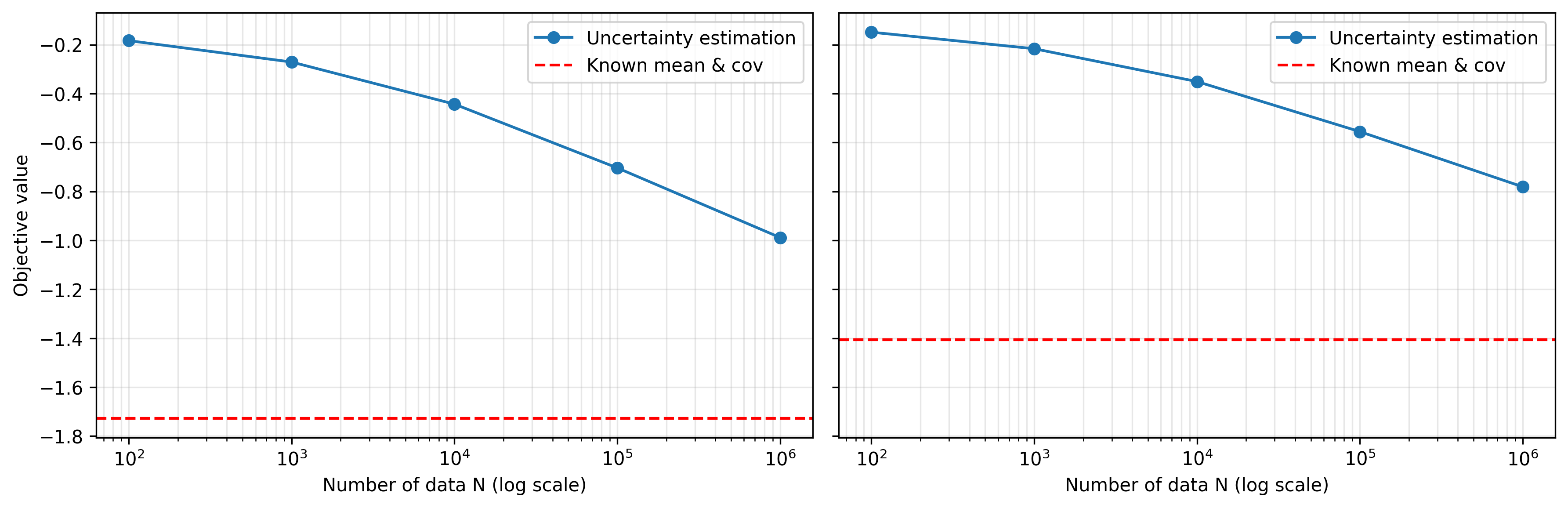
In Figure 5, we investigate the impact of estimation uncertainty. We first generate the true parameters (μd,Γd,Jd)(\mu_{d},\Gamma_{d},J_{d}) and solve the problem assuming they are exactly known (red line). We then generate NN random samples from this distribution and re-solve the problem using the empirical estimates (μ^d,Γ^d,J^d)(\widehat{\mu}_{d},\widehat{\Gamma}_{d},\widehat{J}_{d}) for different values of NN. As the number of samples increases, the resulting objective values gradually converge to those obtained under the true parameters, confirming that the empirical estimates converge to the true distribution as NN grows.

Refer to caption
Figure 5: Effect of estimation uncertainty for the individual (left) and joint (right) formulations (n=10n=10, m=10m=10, p=0.75p=0.75, θ=4\theta=4). The red line corresponds to the solution obtained with the true (μd,Γd,Jd)(\mu_{d},\Gamma_{d},J_{d}).

8 Conclusion

This work developed a unified and tractable framework for the Complex Chance-Constrained Problem (3CP), extending classical chance-constrained formulations to the complex-valued setting. We established deterministic SOCP reformulations for individual chance constraints under general Complex Elliptically Symmetric (CES) distributions, moment-based distributional robustness, bounded-norm uncertainty, and fully data-driven scenarios where only empirical estimates of the mean and covariance are available. To address joint chance constraints, we incorporated dependence via the Gumbel-Hougaard copula and proposed lower and upper SOCP approximations based on first-order Taylor expansions and piecewise linear interpolation in the complex space. Numerical experiments confirmed the theoretical guarantees: for all distributional settings, the empirical violation rates remained below the target level 1−p1-p, and the SOCP upper-lower gap decreased steadily with more tangent points. The data-driven formulation was shown to be stable, with solutions converging to those obtained using the true parameters as the sample size grows. The application to MVDR beamforming demonstrated that the proposed 3CP framework can be directly applied to practical signal processing problems and remains robust to model mismatch. The complex formulation reduces to the classical real-valued chance-constrained problem as a special case. Thus, all the deterministic SOCP reformulations derived for the complex setting naturally contain the real case as a direct special instance.

References

  • Abrams [1972] Robert A Abrams. Nonlinear programming in complex space: Sufficient conditions and duality. Journal of Mathematical Analysis and Applications, 38(3):619–632, 1972. ISSN 0022-247X. doi:https://doi.org/10.1016/0022-247X(72)90073-X.
  • Adasme and Lisser [2019] Pablo Adasme and Abdel Lisser. A variable neighborhood search algorithm for massive mimo resource allocation. In Mobile Web and Intelligent Information Systems, pages 3–15, Cham, 2019. Springer International Publishing. ISBN 978-3-030-27192-3.
  • Ahlfors and Ahlfors [1979] Lars Valerian Ahlfors and Lars V Ahlfors. Complex analysis. McGraw-Hill New York, 1979.
  • Calafiore and Ghaoui [2006] Giuseppe Carlo Calafiore and L El Ghaoui. On distributionally robust chance-constrained linear programs. Journal of Optimization Theory and Applications, 130(1):1–22, 2006. doi:https://doi.org/10.1007/s10957-006-9084-x.
  • Charnes and Cooper [1959] Abraham Charnes and William W Cooper. Chance-constrained programming. Management science, 1959. doi:https://doi.org/10.1287/mnsc.6.1.73.
  • Cheng and Lisser [2012] Jianqiang Cheng and Abdel Lisser. A second-order cone programming approach for linear programs with joint probabilistic constraints. Operations Research Letters, 40(5):325–328, 2012. ISSN 0167-6377. doi:https://doi.org/10.1016/j.orl.2012.06.008.
  • Cheng et al. [2014] Jianqiang Cheng, Erick Delage, and Abdel Lisser. Distributionally robust stochastic knapsack problem. SIAM Journal on Optimization, 24(3):1485–1506, 2014. doi:10.1137/130915315.
  • Cheng et al. [2015] Jianqiang Cheng, Michal Houda, and Abdel Lisser. Chance constrained 0–1 quadratic programs using copulas. Optimization Letters, 2015. doi:https://doi.org/10.1007/s11590-015-0854-y.
  • Cox et al. [1987] H. Cox, R. Zeskind, and M. Owen. Robust adaptive beamforming. IEEE Transactions on Acoustics, Speech, and Signal Processing, 35(10):1365–1376, 1987. doi:10.1109/TASSP.1987.1165054.
  • Ferrero [1992] Oscar Ferrero. On nonlinear programming in complex spaces. Journal of Mathematical Analysis and Applications, 164(2):399–416, 1992. ISSN 0022-247X. doi:https://doi.org/10.1016/0022-247X(92)90123-U.
  • Hoeffding [1963] Wassily Hoeffding. Probability inequalities for sums of bounded random variables. Journal of the American Statistical Association, 58(301):13–30, 1963. ISSN 01621459, 1537274X.
  • Ion et al. [2023] Roxana A Ion, Chris AJ Klaassen, and Edwin R van den Heuvel. Sharp inequalities of bienaymé–chebyshev and gauß type for possibly asymmetric intervals around the mean. Test, 32(2):566–601, 2023. doi:https://doi.org/10.1007/s11749-022-00844-9.
  • Kreutz-Delgado [2009] Ken Kreutz-Delgado. The complex gradient operator and the cr-calculus. arXiv preprint arXiv:0906.4835, 2009.
  • Lauro et al. [2025] Luigi Di Lauro, Stefania Sciara, Bennet Fischer, Junliang Dong, Imtiaz Alamgir, Benjamin Wetzel, Goëry Genty, Mitchell Nichols, Armaghan Eshaghi, David J. Moss, and Roberto Morandotti. Optimization methods for integrated and programmable photonics in next-generation classical and quantum smart communication and signal processing systems. Adv. Opt. Photon., 17(3):526–622, Sep 2025. doi:10.1364/AOP.533504.
  • Levinson [1966] Norman Levinson. Linear programming in complex space. Journal of Mathematical Analysis and Applications, 14(1):44–62, 1966. ISSN 0022-247X. doi:https://doi.org/10.1016/0022-247X(66)90061-8.
  • Liu et al. [2016] Jia Liu, Abdel Lisser, and Zhiping Chen. Stochastic geometric optimization with joint probabilistic constraints. Operations Research Letters, 44(5):687–691, 2016. ISSN 0167-6377. doi:https://doi.org/10.1016/j.orl.2016.08.002.
  • Liu et al. [2022] Jia Liu, Abdel Lisser, and Zhiping Chen. Distributionally robust chance constrained geometric optimization. Mathematics of Operations Research, 47(4):2950–2988, 2022. doi:10.1287/moor.2021.1233.
  • Madani and Lisser [2026] Raneem Madani and Abdel Lisser. Chance constrained optimization with complex variables. In Optimization and Learning, pages 279–290. Springer Nature Switzerland, 2026. ISBN 978-3-032-13589-6. doi:https://doi.org/10.1007/978-3-032-13589-6_21.
  • Madani et al. [2026] Raneem Madani, Abdel Lisser, and Zeno Toffano. Data-driven joint complex-valued chance-constrained programs under wasserstein ambiguity set. HAL preprint, hal-05536419, 2026.
  • Marshall and Olkin [1960] Albert W. Marshall and Ingram Olkin. Multivariate Chebyshev Inequalities. The Annals of Mathematical Statistics, 31(4):1001 – 1014, 1960. doi:10.1214/aoms/1177705673.
  • Middleton [1973] D. Middleton. Man-made noise in urban environments and transportation systems: Models and measurements. IEEE Transactions on Communications, 21(11):1232–1241, 1973. doi:10.1109/TCOM.1973.1091566.
  • Nelsen [2006] Roger B Nelsen. An introduction to copulas. Springer, 2006. doi:https://doi.org/10.1007/0-387-28678-0.
  • Nguyen et al. [2023] Hoang Nam Nguyen, Abdel Lisser, and Jia Liu. Convexity of linear joint chance constrained optimization with elliptically distributed dependent rows. Results in Control and Optimization, 12:100285, 2023. ISSN 2666-7207. doi:https://doi.org/10.1016/j.rico.2023.100285.
  • Novey et al. [2010] Mike Novey, Tülay Adali, and Anindya Roy. A complex generalized gaussian distribution— characterization, generation, and estimation. IEEE Transactions on Signal Processing, 58(3):1427–1433, 2010. doi:10.1109/TSP.2009.2036049.
  • Ollila and Koivunen [2004] E. Ollila and V. Koivunen. Generalized complex elliptical distributions. In Processing Workshop Proceedings, 2004 Sensor Array and Multichannel Signal, pages 460–464, 2004. doi:10.1109/SAM.2004.1502990.
  • Ollila et al. [2012] Esa Ollila, David E. Tyler, Visa Koivunen, and H. Vincent Poor. Complex elliptically symmetric distributions: Survey, new results and applications. IEEE Transactions on Signal Processing, 60(11):5597–5625, 2012. doi:10.1109/TSP.2012.2212433.
  • Peng et al. [2024] Zhangjie Peng, Zhibo Zhang, Cunhua Pan, Marco Di Renzo, Octavia A. Dobre, and Jiangzhou Wang. Beamforming optimization for active ris-aided multiuser communications with hardware impairments. IEEE Transactions on Wireless Communications, 23(8):9884–9898, 2024. doi:10.1109/TWC.2024.3367131.
  • Rahimian and Mehrotra [2022] Hamed Rahimian and Sanjay Mehrotra. Frameworks and Results in Distributionally Robust Optimization. Open Journal of Mathematical Optimization, 3:4, 2022. doi:10.5802/ojmo.15.
  • Schreier and Scharf [2003] P.J. Schreier and L.L. Scharf. Second-order analysis of improper complex random vectors and processes. IEEE Transactions on Signal Processing, 51(3):714–725, 2003. doi:10.1109/TSP.2002.808085.
  • Sorber et al. [2012] Laurent Sorber, Marc Van Barel, and Lieven De Lathauwer. Unconstrained optimization of real functions in complex variables. SIAM Journal on Optimization, 22(3):879–898, 2012. doi:10.1137/110832124.
  • Tassouli and Lisser [2023] Siham Tassouli and Abdel Lisser. Maximizing signal to interference noise ratio for massive mimo: A stochastic neurodynamic approach. In Mobile Web and Intelligent Information Systems, pages 221–234, Cham, 2023. Springer Nature Switzerland. ISBN 978-3-031-39764-6.
  • Varagapriya et al. [2025] V Varagapriya, Vikas Vikram Singh, and Abdel Lisser. Convex approximations of random constrained markov decision processes. SIAM Journal on Optimization, 35(3):1703–1730, 2025. doi:10.1137/24M1660711.
  • Zhang and Huang [2006] Shuzhong Zhang and Yongwei Huang. Complex quadratic optimization and semidefinite programming. SIAM Journal on Optimization, 16(3):871–890, 2006. doi:10.1137/04061341X.