Improved Torn Paper Coding via Local Alignment

Since our method is similar to the interleaved pilot scheme of [12], we introduce it here as the basis for our refined construction in Section III-B. We begin with the definition of a De Bruijn sequence.

For a fixed positive integer $m$, consider a De Bruijn sequence $\mathbf{p}$ of length $n/m$, which we refer to as the pilot sequence. According to Definition 1, every sequence of length $\log(n/m)$ appears in $\mathbf{p}$ exactly once. To construct the codebook, the authors of [12] interleave the pilot sequence with codewords of an erasure code. Specifically, let $\mathcal{C}_{\mathrm{er}}$ be an erasure code of length $n/m$ and rate $R_{\mathrm{er}}$. They form a shifted version of this code by drawing an i.i.d. $\mathrm{Ber}(1/2)$ random vector in $\{0,1\}^{n/m}$ and XORing it with each codeword of $\mathcal{C}_{\mathrm{er}}$, thereby obtaining the pseudo-random code $\tilde{\mathcal{C}}_{\mathrm{er}}$. A key property required for successful global alignment is that the pilot sequence substrings should not coincide with any substring of a randomly shifted erasure codeword as follows.

Observation 1 is proved via a straightforward application of the union bound. Therefore, if $k=(2+\delta)\log n$ for some $\delta>0$, this probability goes to $0$ when $n\xrightarrow[]{}\infty$. This means that for any $\epsilon>0$ there exists a large enough $n$ so that it is possible to choose at least a $1-\epsilon$ fraction of the codewords in $\tilde{\mathcal{C}}_{\mathrm{er}}$ such that any $(2+\delta)\log n$ segment in any of its codewords is distinct from any $(2+\delta)\log n$ segment of the pilot sequence $\mathbf{p}$.

Let $\mathcal{S}=\{\mathbf{s}_{1},\mathbf{s}_{2},\dots,\mathbf{s}_{|\mathcal{S}|}\}\subset\tilde{\mathcal{C}}_{\mathrm{er}}$ be a set of $(1-\epsilon)2^{\frac{n}{m}R_{\mathrm{er}}}$ such codewords, i.e., where none of them shares any $(2+\delta)\log n$ contiguous subsequence with $\mathbf{p}$. Ref. [12] builds a codeword $\mathbf{c}$ by taking $m-1$ codewords from $\mathcal{S}$ and interleaving their symbols with symbols from $\mathbf{p}$. More precisely, for any function $u:[m-1]\to[|\mathcal{S}|]$, they build the codeword $\mathbf{c}_{u}=(\mathbf{c}_{u}[0],\mathbf{c}_{u}[1],\ldots,\mathbf{c}_{u}[n-1])$ where for every $t\in\{0,1,\dots,n/m-1\}$, we have

The resulting codebook is of size $|\mathcal{S}|^{m-1}=(1-\epsilon)^{m-1}2^{(1-\frac{1}{m})nR_{\mathrm{er}}}$.

Subsequently, decoding begins by recovering the global alignment of the fragments through the periodically embedded pilot symbols drawn from the De Bruijn sequence $\mathbf{p}$. Since a window of length $(2+\delta)\log n$ from the pilot sequence coincides with a window of the shifted erasure code with probability which tends to zero as $n\to\infty$, every fragment whose length exceeds $(2+\delta)m\log n$ must contain at least one pilot window of length $(2+\delta)\log n$ that is uniquely identifiable. Moreover, because every $\log(n/m)$ window of the De Bruijn sequence $\mathbf{p}$ is distinct, the occurrence of such a window immediately reveals the fragment’s absolute position in the codeword, a process we call global alignment. Once these long fragments are anchored, the short fragments—those too small to contain any identifiable pilot window—are discarded, and the resulting missing positions are treated as erasures. The reconstruction of the full message is then completed by the outer shifted-erasure code $\tilde{\mathcal{C}}_{\mathrm{er}}$, which deterministically corrects the erased locations created by the random breaking process.

Notice that in the interleaved-pilot scheme, the decoder identifies the locations of the pilot sequence bits only in sufficiently long fragments. The rationale is that the probability of a long window of the De Bruijn sequence coinciding with a window of any shifted erasure codeword is vanishingly small. However, this approach has an inherent gap: the number of bits required to ensure that a De Bruijn window is not identical to a shifted erasure codeword window is approximately $2\log n$ (Observation 1), whereas the number of bits needed to uniquely identify a De Bruijn window is only $\log(n/m)$. Consequently, the decoder in [12] restricts itself to fragments of length at least $(2+\delta)m\log n$, discarding the large number of shorter fragments, which reduces the effective rate since all such fragments are treated as erasures.

This observation motivates the question of whether one can identify the locations of the pilot sequence bits by exploiting the local pattern surrounding each De Bruijn bit, rather than relying solely on long fragments. Specifically, we embed a small deterministic marker into the De Bruijn sequence and actively prevent this marker from appearing within the erasure code. By detecting these distinct structural patterns within any given fragment, we can distinguish the De Bruijn bits from the erasure-coded bits—a technique we term local alignment. Once this pattern is identified, the De Bruijn window can be reliably inferred. This enables the decoder to determine the global position of fragments whose lengths are well below $(2+\delta)m\log n$.

Since our method uses an RLL technique for local alignment, we introduce it here as the basis for our construction in Section III-B. The codewords of an RLL code are binary sequences of a fixed length $n$, characterized by parameters $d$ and $k$. These parameters indicate the minimum and maximum number of $0$’s between consecutive $1$’s in the sequence. For example, an $\text{RLL}(1,3)$ code, also known as Modified Frequency Modulation (MFM) [6], requires that between any two $1$’s there are at least $d=1$ and at most $k=3$ $0$’s. To meet the requirements of Section III-B which follows, we require an $\mathrm{RLL}(0,k-1)$ scheme and an $\mathrm{RLL}(0,k-2)$ scheme, which are obtained by insertion of $1$’s into the information words, and are introduced in the following simple lemmas.

While Lemma 1 established the existence of an $\mathrm{RLL}(0,k-1)$ fixed-length block code with rate $\frac{k-1}{k}$, the following lemma introduces an $\mathrm{RLL}(0,k-2)$ fixed-length block code achieving a rate of $\frac{k-2}{k}$.

Lemmas 1 and 2 demonstrate two distinct methods for constructing fixed-length block codes that achieve an asymptotic rate of $1$ as $k\to\infty$. Furthermore, these two constructions are tailored to serve different purposes within the overall encoding process in Section III-B. To simplify our exposition and explicitly distinguish between these two schemes, we adopt the following terminology:

• •

  We refer to the $\mathrm{RLL}(0,k-1)$ fixed-length block code with rate $\frac{k-1}{k}$ from Lemma 1 as the $\mathrm{RLL}(0,k-1)$ code, and its corresponding operations as the $\mathrm{RLL}(0,k-1)$ encoder and decoder.

• •

  We refer to the $\mathrm{RLL}(0,k-2)$ fixed-length block code with rate $\frac{k-2}{k}$ from Lemma 2 as the $\widetilde{\mathrm{RLL}}(0,k-2)$ code, and its corresponding operations as the $\widetilde{\mathrm{RLL}}(0,k-2)$ encoder and decoder.

The encoding process starts with an inner code designed to align fragments. Once fragments are aligned, their missing lengths and positions are known, making this fundamentally an erasure channel (see proofs in Section III-D). By employing a random binary linear code, we can recover these erasures efficiently in polynomial time—essentially by using Gaussian elimination to solve a system of linear equations over $\mathbb{F}_{2}$. The parameters for this code are defined below.

The following lemma proves that the matrix $H$ achieves full row rank with high probability, thereby establishing the rate of $\mathcal{C}_{\mathrm{er}}$.

With $\mathcal{C}_{\mathrm{er}}$ established, the next step in the encoding process is constructing the pilot sequence. Let $\mathbf{q}$ be a De Bruijn sequence of length $\frac{n}{m}(1-\frac{\beta}{(1+\delta/2)\log n})\frac{\beta-2}{\beta}$, where $\delta$ is a small constant that satisfies $\delta>\frac{2}{\beta-2}$ and $\beta$ is as in Definition 2, i.e. $\beta=o(\log(n))$ and $\beta=\omega(1)$. This sequence $\mathbf{q}$ has the property that every sequence of length $\log(\frac{n(\beta-2)}{m\beta}(1-\frac{\beta}{(1+\delta/2)\log n}))$ appears in $\mathbf{q}$ exactly once. Subsequently, we apply the $\widetilde{\text{RLL}}(0,\beta-2)$ encoder from Lemma 2 to $\mathbf{q}$, yielding a modified De Bruijn sequence $\bar{\mathbf{q}}$ of length $\frac{n}{m}(1-\frac{\beta}{(1+\delta/2)\log n})$. For simplicity, we further assume that $\beta|(1+\delta/2)\log n$ and define the modified pilot sequence $\mathbf{p}$ as follows.

In Definition 3 we systematically embed runs of $\beta$ consecutive zeros, called markers, at fixed intervals throughout the pilot sequence $\mathbf{p}$. The process of constructing $\mathbf{p}$ from the De Bruijn sequence $\mathbf{q}$ is therefore:

Based on this process, we establish the following key property of $\mathbf{p}$.

Next, we apply the $\text{RLL}(0,\beta-1)$ fixed-length block encoding algorithm from Lemma 1 to all codewords of $\mathcal{C}_{\mathrm{er}}$, yielding a code $\bar{\mathcal{C}}_{\mathrm{er}}$; the block length of $\bar{\mathcal{C}}_{\mathrm{er}}$ is $n/m$ and its rate is $(1-\frac{1}{\beta})R_{\mathrm{er}}$ and hence its size is $2^{\frac{n}{m}(1-\frac{1}{\beta})R_{\mathrm{er}}}$. To construct the final code, we interleave the pilot sequence $\mathbf{p}$ with the codewords of $\bar{\mathcal{C}}_{\mathrm{er}}$ in a manner that resembles the interleaving from [12] given in Section II-A. Rather than interleaving $m-1$ codewords from a subset of a random coset of $\mathcal{C}_{\mathrm{er}}$ (which has no substring intersection with their pilot sequence) with a De Bruijn sequence as done in [12], we interleave $m-1$ codewords of $\bar{\mathcal{C}}_{\mathrm{er}}$ with our pilot sequence (Definition 3).

Formally, we fix an arbitrary indexing $\bar{\mathcal{C}}_{\mathrm{er}}=\{\bar{\mathbf{s}}_{1},\ldots,\bar{\mathbf{s}}_{|\bar{\mathcal{C}}_{\mathrm{er}}|}\}$, and write our code as

where for each $t\in\{0,1,\dots,n/m-1\}$,

Since the encoding process above is injective (i.e., $\mathbf{c}_{v}\neq\mathbf{c}_{v^{\prime}}$ whenever $v\neq v^{\prime}$), the size of the resulting $\mathcal{C}$ (3) is $|\bar{\mathcal{C}}_{\mathrm{er}}|^{m-1}=(2^{\frac{n}{m}(1-\frac{1}{\beta})R_{\mathrm{er}}})^{m-1}=2^{(1-\frac{1}{\beta})(1-\frac{1}{m})nR_{\mathrm{er}}}$. Since $\beta=o(\log(n))$ and $\beta=\omega(1)$, we have

and hence the resulting rate tends to $\left(1-1/m\right)R_{\mathrm{er}}$ as $n$ tends to infinity, i.e.,

The decoding process essentially reduces the torn paper channel into a (not memoryless) erasure channel by exploiting the interleaved structure of codewords. At a high level, this is achieved through a three-step procedure:

1. A

   Local Alignment: The decoder identifies the positions of the $\mathbf{p}$ bits (see (2)) within all fragments of length at least $(1+\delta)m\log n$ and discards all other fragments. For each such fragment, this is done by first de-interleaving it to obtain sequences $\mathbf{w}_{0},\ldots,\mathbf{w}_{m-1}$, and identifying the unique $\mathbf{w}_{j}$ which contains $0$-runs of length $\beta$ as the one which contains bits from $\mathbf{p}$.

2. B

   Global Alignment: In each sufficiently long fragment, we remove the $0$-runs of length $\beta$ from the $\mathbf{w}_{j}$ found in step A, obtaining a substring from $\bar{\mathbf{q}}$, which is then decoded to obtain a substring of $\mathbf{q}$ (again see (2)). This substring of $\mathbf{q}$—being a De Bruijn subsequence—is used to determine the unique global position of the fragment.

3. C

   RLL and Erasure Decoding: After global alignment, we obtain an estimate $\hat{\mathbf{c}}_{v}$ of $\mathbf{c}_{v}$, and extract substrings of the codewords in $\bar{\mathcal{C}}_{\mathrm{er}}$ from $\hat{\mathbf{c}}_{v}$ (see (4)). These substrings are processed by an RLL decoding algorithm to remove run-length constraints, followed by standard erasure decoding for $\mathcal{C}_{\mathrm{er}}$ to recover the original message.

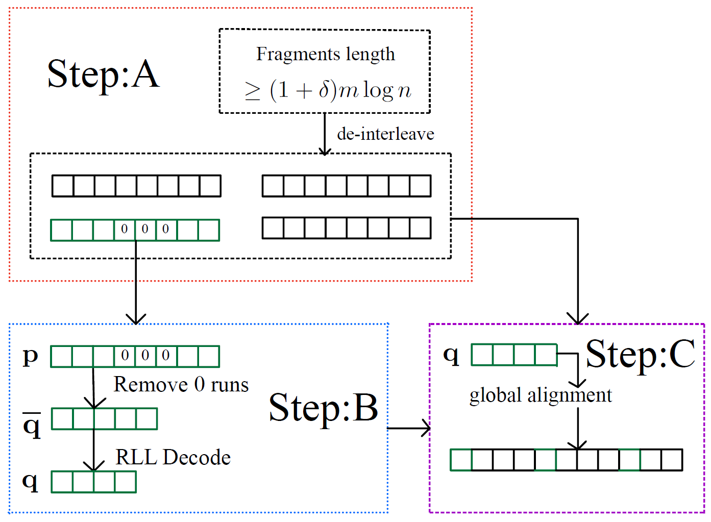
Step A (local alignment) is detailed in Algorithm 1, whose correctness is established in Lemma 5 below. Throughout the proof, recall that a transmitted word $\mathbf{c}_{v}$ is obtained by interleaving $\mathbf{p}$ with codewords $\bar{\mathbf{s}}_{v(1)},\ldots,\bar{\mathbf{s}}_{v(m-1)}$ from $\bar{\mathcal{C}}_{\text{er}}$ for some $v:[m-1]\to|\bar{\mathcal{C}}_{\text{er}}|$. Additionally, let $\mathcal{F}$ be the set of all fragments whose length is at least $(1+\delta)m\log n$.

Once the bits $\mathbf{p}_{\mathbf{f}}$ of the pilot sequence $\mathbf{p}$ and the bits $\mathbf{y}_{\mathbf{f}}^{i}$ of every $\bar{\mathbf{s}}_{v(i)}$ have been located within every fragment, step A (local alignment) is concluded. Then, step B (global alignment) is conducted via the following sub-steps, which are executed in Algorithm 2.

1. B1

   Extraction of modified De Bruijn sequence bits: For every $\mathbf{f}\in\mathcal{F}$, we identify and extract the substring $\bar{\mathbf{q}}_{\mathbf{f}}$ of $\bar{\mathbf{q}}$ inside $\mathbf{p}_{\mathbf{f}}$.

2. B2

   Extraction of De Bruijn sequence bits: For every $\mathbf{f}\in\mathcal{F}$, we run the $\widetilde{\mathrm{RLL}}(0,\beta-2)$ decoder over $\bar{\mathbf{q}}_{\mathbf{f}}$ to extract the bits $\mathbf{q}_{\mathbf{f}}$ of $\mathbf{q}$ inside $\mathbf{p}_{\mathbf{f}}$.

3. B3

   Perform global alignment: Determine the global positions of every $\mathbf{f}\in\mathcal{F}$ using $\mathbf{q}_{\mathbf{f}}$.

The correctness of steps B1 and B2 is proved in Lemma 6 and Lemma 7; the fact that $\mathbf{q}_{\mathbf{f}}$ is sufficiently long to conduct B3 is proved in Lemma 8.

By Lemma 6, the bits corresponding to the modified De Bruijn sequence $\bar{\mathbf{q}}_{\mathbf{f}}$ can be identified and extracted from every $\mathbf{f}\in\mathcal{F}$. Following that, we apply an $\widetilde{\mathrm{RLL}}(0,\beta-2)$ decoder over $\bar{\mathbf{q}}_{\mathbf{f}}$ to obtain the De Bruijn sequence bits $\mathbf{q}_{\mathbf{f}}$, (Line 7), and use $\mathbf{q}_{\mathbf{f}}$ for global alignment. The detailed process is given in Algorithm 2 and proved in Lemma 7.

Next, we show that $\mathbf{q}_{\mathbf{f}}$ identified in Lemma 7 can be used for global alignment, thereby proving the correctness of B3.

Finally, RLL and erasure decoding (step C) is executed via the following sub-steps, which are implemented in Algorithm 3 and proved in Lemma 9 below.

1. C1

   Removal of $\mathrm{RLL}$-added bits: The output of step B3 is an estimated codeword $\hat{\mathbf{c}}_{v}$, which contains all fragments $\mathbf{f}\in\mathcal{F}$ placed in their correct global positions, and erasures (say, $\star$ symbols) in all other positions. Since the $\mathrm{RLL}(0,\beta-1)$ encoder inserts $1$’s at prescribed locations, these positions are known from the construction. We remove all such positions from $\hat{\mathbf{c}}_{v}$, resulting in a partially observed version of the interleaved codewords from $\mathcal{C}_{\mathrm{er}}$.

2. C2

   De-interleaving: After removing the $\mathrm{RLL}$-added bits, we de-interleave the resulting sequence to obtain estimates $\hat{\mathbf{r}}_{v(1)},\hat{\mathbf{r}}_{v(2)},\dots,\hat{\mathbf{r}}_{v(m-1)}$ of the codewords in $\mathcal{C}_{\mathrm{er}}$ used to construct $\mathbf{c}_{v}$ as in (4). Each $\hat{\mathbf{r}}_{v(i)}$ contains erasures in positions that were not covered by sufficiently long fragments.

3. C3

   Erasure decoding: For each $\hat{\mathbf{r}}_{v(1)},\hat{\mathbf{r}}_{v(2)},\dots,\hat{\mathbf{r}}_{v(m-1)}$, we apply standard erasure decoding.

We comment that steps C1 and C2 above are implemented in Algorithm 3 via a linear pass over the bits of each fragment (Lines 4-12), while skipping $\textrm{RLL}(0,\beta-1)$ bits (Line 8) and sorting the remaining bits to $\mathcal{C}_{\text{er}}$ codewords (Line 9). The proof of correctness of Algorithm 3 is as follows.

References

- [1] (2020) Low cost dna data storage using photolithographic synthesis and advanced information reconstruction and error correction. Nature communications 11 (1), pp. 5345. Cited by: §I.
- [2] (2023) Adversarial torn-paper codes. IEEE Trans. on Inf. Th. 69 (10), pp. 6414–6427. Cited by: §I.
- [3] (2016) Forward error correction for dna data storage. Procedia Computer Science 80, pp. 1011–1022. Cited by: §I.
- [4] (2012) A logic-gated nanorobot for targeted transport of molecular payloads. Science 335 (6070), pp. 831–834. Cited by: §I.
- [5] (2013) Towards practical, high-capacity, low-maintenance information storage in synthesized DNA. nature 494 (7435), pp. 77–80. Cited by: §I.
- [6] (1990) Runlength-limited sequences. Proceedings of the IEEE 78 (11), pp. 1745–1759. Cited by: §III-A.
- [7] (2025) Efficient nested hash reassembly codes for torn paper channels. IEEE Transactions on Communications. Cited by: §I, §II.
- [8] (2026) Improvement for torn paper codes by local alignment technique. 2026 IEEE Intl. Symp. on Inf. Th. (ISIT). Cited by: Figure 1, §I, §III-E.
- [9] (2025) Single fragment forensic coding from van der corput sets. In 2025 IEEE International Symposium on Information Theory (ISIT), pp. 1–6. Cited by: §I.
- [10] (2023) DNA merge-sort: a family of nested varshamov-tenengolts reassembly codes for out-of-order media. IEEE Transactions on Communications 72 (3), pp. 1303–1317. Cited by: §I, §II.
- [11] (2024) Recovering a message from an incomplete set of noisy fragments. arXiv preprint arXiv:2407.05544. Cited by: §I, §I, §II, §IV, §IV, §IV, Lemma 13.
- [12] (2021) Torn-paper coding. IEEE Transactions on Information Theory 67 (12), pp. 7904–7913. Cited by: Figure 1, §I, §I, §I, §I, §II-A, §II-A, §II-A, §II-A, §II, §II, §II, §III-B, §III-E, TABLE I, TABLE I, TABLE I, Definition 5, Lemma 15.
- [13] (2023) Error correction for DNA storage. IEEE BITS the Inf. Th. Magazine 3 (3), pp. 78–94. Cited by: §I.
- [14] (2024) Break-resilient codes for forensic 3d fingerprinting. In 2024 IEEE Intl. Symp. on Inf. Th. (ISIT), pp. 3148–3153. Cited by: §I.
- [15] (2025) Secure information embedding and extraction in forensic 3d fingerprinting. USENIX Security. Cited by: §I, §II.
- [16] (2026) Directionality (molecular biology) — Wikipedia, the free encyclopedia. Note: [Online; accessed 31-March-2026] External Links: Link Cited by: §II.
- [17] (2026) Dominated convergence theorem — Wikipedia, the free encyclopedia. Note: [Online; accessed 4-June-2026] External Links: Link Cited by: footnote 2.
Appendix A Omitted proof
Proof of Lemma 10.
Fix , let , and let denote the submatrix of formed by the columns indexed by . A binary linear code successfully decodes the erasure pattern if and only if the columns of are linearly independent, which is equivalent to . Since the entries of are chosen independently and uniformly from , we can analyze the linear independence of by building the submatrix column by column. Conditioned on the first columns being linearly independent, their span contains exactly vectors out of the vectors in . The probability that the -th randomly chosen column belongs to this span (an individual failure) is .
Since rank deficiency occurs if any individual column belongs to the span of its predecessors, we can apply the union bound to sum these individual failure probabilities. Thus, the probability that is rank deficient is at most:
Since and , it follows that , and hence we obtain the bound . Since where , , and , we have that whenever . Therefore, since , this failure probability tends to zero exponentially fast when . ∎
Appendix B Proofs regarding good erasure patterns
In this appendix, we show that the erasure pattern induced by the torn paper channel belongs to (see (7)) with probability tending to as . The following Definition 5, Lemma 14 and Lemma 15 are used to prove Lemma 16.
Definition 5.
[12, Definition 1] For a constant , the coverage is the fraction of output bits which reside in fragments of length at least , i.e.,
where is the indicator function of the event .
Lemma 14.
Let be the smallest index such that
where are i.i.d. random variables representing the lengths of broken fragments. Then
with high probability.
Proof.
For each , let be the indicator of the event that a break occurred between and . Then
and the random variables are independent. Since every break increases the number of fragments by one, we have
Since , there exists a constant such that, for all sufficiently large ,
and hence
By Chernoff’s bound, for all sufficiently large ,
which tends to zero as . Therefore, with high probability,
Lemma 15.
[12, Lemma 6] For a constant , the coverage satisfies the following two properties