Signatures of the Quantum Geometric Dipole of Interlayer Excitons in Counterflow Conductivity
Abstract
Collective excitations of many-body electron systems can carry internal structure, supporting novel quantum geometric and topological properties. Among these are a quantum geometric dipole (QGD), which for excitons have direct significance as an internal polarization. For interlayer excitons of a bilayer system, this represents an in-plane dipole moment, which can be used to drive them with in-plane electric fields. In this work, we consider counterflow electric currents associated with driven excitons in such a bilayer system as a probe of their QGD structure. As a simple but non-trivial example, we analyze a structure with a one-dimensional periodic potential in a strong perpendicular magnetic field. The resulting magnetoexciton bands host QGD structure that distinguishes it from the exciton QGD of a uniform system. To model exciton transport we adopt a Boltzmann approach that includes inter-band tunneling, allowing us to consider non-equilibrium momentum distributions that result from strong layer-antisymmetric driving fields. We show how linear response to a layer-symmetric component of the driving fields provide information about the QGD, and that the broad QGD structure of the exciton bands can be probed by the varying the layer-antisymmetric field. Our results demonstrate that counterflow conductivity serves as a tunable probe of the internal quantum geometric structure carried by the interlayer excitons, connecting transport to the quantum geometry of many-body excitations.
I Introduction
The emergence of two-dimensional Van der Waals (vdW) materials has in recent years allowed the realization of a number of exotic electron states in a variety of multilayer systems [1, 2, 3, 4]. These systems host striking behaviors made possible by the effects of electron-electron interactions on the system, including correlated insulators, superconducting states, magnetic states, and integer and fractional Chern insulators [5, 6, 7, 8, 9, 10, 11, 12, 13]. In many of these states, quantum geometry plays a crucial role, and the unusual behavior this brings is enriched by interactions among the electrons. The role of these interactions can be important both within and across layers.
For insulating states – typically semiconductors – a fundamental marker of interaction effects is the presence of exciton states in the low-energy spectrum of the system [14, 15]. Excitons are bound particle-hole excitations akin to hydrogen atoms, in which the electronic structure of the electron and hole bands have important qualitative effects [16, 17]. In two-dimensional materials such as van der Waals layers, they are often particularly low in energy (i.e., more strongly bound) than is the case for bulk materials, due to the relatively weak screening of the Coulomb interaction by the material itself [18, 19]. While band energetics have long been known to impact exciton energies and behaviors, it has more recently been appreciated that the quantum geometries of these bands impact the exciton properties as well [20, 21]. Indeed, as collective modes with well-defined momenta, exciton states have their own quantum geometries [22, 23], and because of their internal structure they admit a richer set of quantum geometric characterizations than is possible for single-electron bands [24].
In this work, we focus on a unique quantum geometric property of excitons: their quantum geometric dipole (QGD) [25]. This is an internal polarization of the exciton that is tied to its momentum in the Hilbert space of an exciton band [26, 27, 28, 29, 30]. Direct analogs of this quantum geometric structure may also be found in magnons [31] and plasmons [32, 33]. Of particular interest in this context are interlayer excitons, in which the electron and hole reside in different layers of a multilayer structure. The segregation of the constituents into these separate spaces endows the exciton with attractive properties and possibilities: control of its energy with perpendicular electric field [34], enhanced lifetime due to the physical separation between the particle and hole [35], and the possibility of applying different electric fields in the two layers, yielding different forces on the electron and hole [36, 37, 38, 39]. In vdW materials, such interlayer excitons have been realized [34, 35, 40] in pairs of transition metal dichalcogenide (TMD) layers separated by one or more layers of hexagonal boron nitride (hBN), for which tunneling between the layers is negligibly small. Analogous systems may be fabricated using graphene layers to host electrons and holes, with a strong magnetic field introducing gaps in their electronic spectra [38, 39]. In this latter case, the relevant excitations are magnetoexcitons.


The connection between the electric dipole moment of a magnetoexciton in the strong field limit and its momentum is well-known[41, 42, 43, 44], but more recently this connection has been reinterpreted and generalized to other systems from a quantum geometric perspective [24, 45]. One consequence of this is that the semiclassical dynamical equation of motion of an exciton wave packet is influenced by quantum geometry not just through the anomalous velocity associated with the Berry’s curvature, but also through a drift velocity [24, 26] associated with the QGD. The consequences of this are largely unexplored and are the subject of this study. Specifically, we develop a Boltzmann approach to counterflow conductivity carried by a collection of interlayer excitons, focusing on contributions from the QGD. By exploiting the freedom to consider different in-plane components of the electric field in each layer (see Fig. 1), we show it is possible to vary the momentum distribution of the interlayer excitons (through a strong layer-antisymmetric component of the electric field) while isolating the contribution of the QGD to counterflow transport (via linear response to a layer-symmetric electric field component). We solve these equations for the specific case of a collection of interlayer magnetoexcitons in the strong magnetic field limit, subject to a unidirectional periodic potential that introduces an exciton band structure with an associated QGD profile for each band (see Fig. 2.) We show that the counterflow conductivity provides information on how the QGD evolves as higher bands are occupied, through increasingly strong antisymmetric driving fields. We note that, analogously, semiclassical transport has been explored as an indicator for Berry’s curvature effects in both Bloch electrons and excitons [46, 47, 48, 49, 50, 51, 52]. Indeed, non-linear transport of electrons through a band structure has recently been proposed as a probe that indirectly maps its Berry’s curvature profile [53].
Transport of interlayer excitons naturally leads to counterflow currents in a bilayer: when moving in real space, the motion of the particle and hole constituents in their respective layers represents oppositely directed electric currents [54, 55, 56, 57, 58, 59]. The transverse component of this counterflow current is quantified by , the linear response to an interlayer symmetric electric field. As we show below, this quantity is an average of the derivative of the QGD with respect to the crystal momentum along the periodic potential axis, and it depends non-trivially on both the strength of the periodic potential and the antisymmetric component of the electric field. In general, we find that increasing the periodic potential magnitude tends to suppress , in accord with the accompanying suppression of the QGD one finds for the low-lying bands (see Fig. 2b.) By contrast, increasing the layer - antisymmetric driving field enhances , as the exciton population moves to higher energy states, which on average host higher QGD slopes. In this way, the transverse counterflow conductivity provides information about the QGD structure hosted by the exciton bands.


The remainder of this article is organized as follows. In Sec. II.1 we review the QGD and its connection to the exciton electric dipole moment. Section II.2 presents the semiclassical equations of motion for the band-projected exciton dynamics, and how the QGD of interlayer magnetoexcitons of a two-dimensional bilayer in the presence of a unidirectional periodic potential enters them. In Section II.3 we discuss counterflow conductivity from exciton transport and how this can be described in terms of the exciton QGD and a Boltzmann distribution of excitons. We complete our formal discussion in Section II.4, where we explain our approach to computing the multi-band Boltzmann distribution, including interband tunneling in the model. Section III presents numerical results that emerge from our formalism. We conclude with a summary and discussion of our results in Section IV. In addition, we provide details of our calculations in two appendices. Appendix A provides details of our band structure and QGD calculations. Appendix B supplies further details of our counterflow conductivity calculations.
II General Formulation
II.1 Quantum Geometric Dipole
We begin by briefly reviewing the derivation of the QGD and its connection to the internal electric dipole moment of an exciton. We define as the two-body wavefunction for the exciton, where and are the hole and electron positions and is the total exciton momentum. Cell-periodic functions may be constructed via a family of mappings of the form
| (1) |
This construction takes account of the internal structure of an exciton state, with specific form determined by the parameter . For the connection associates the Bloch phase solely with the hole (electron), allowing one to define Berry’s connections specific to each constituent,
| (2) |
| (3) |
where and are the connections associated with electron and hole, respectively. The electric dipole moment may then be shown [24] to obey , where . Because of its quantum geometric construction, the latter quantity is referred to as the quantum geometric dipole (QGD). Note that, while (as usual) the Berry connections are gauge-dependent, their difference is gauge-invariant. Thus, the in-plane dipole moment of a two-dimensional exciton may be understood as being entirely determined by the quantum geometry of the excitonic wavefunctions, as illustrated in Fig. 1b. The QGD produces a correction to the exciton velocity beyond that of the Berry’s curvature, as we discuss below.
While the existence of an internal dipole moment is well-established for magnetoexcitons in a strong magnetic field [24, 25], its interpretation in terms of quantum geometric quantities suggests that it is not limited to this setting. We emphasize that the formulation of is quite general, and applies to any collective mode that can be labeled by and continuously evolves with a well-defined momentum , making it a broadly applicable quantum geometric quantity [25]. Nevertheless, because of its relative analytical simplicity, in what follows we focus on a system of interlayer magnetoexcitons in a two-layer system, subject to a unidirectional periodic potential. Exciton currents in such systems naturally manifest counterflow electric currents [54, 56, 58], and our goal in this study is to understand how exciton QGD’s impact these currents. We thus turn next to their dynamics.
II.2 Semiclassical Equations of motion
Our starting point is the band-projected semiclassical theory of interlayer exciton dynamics in a two-layer system. The equations of motion for the center of mass position and average momentum of an exciton wavepacket are given by [24]
| (4) |
| (5) |
where is the effective Berry’s curvature for the exciton, are the symmetric and antisymmetric combinations of the electric fields applied to the hole and electron layers respectively, is the exciton energy dispersion, and is the exciton quantum geometric dipole. Note in these expressions, the subscript is a band index. It is important to note that the exciton equations of motion involve three quantities that are specific to the particular system they are describing: the energy dispersion , the Berry’s curvature , and the quantum geometric dipole . In the case of magnetoexcitons in a strong magnetic field, for exciton constituents confined to the lowest Landau levels, a non-trivial band structure can be induced via the insertion of a periodic potential, which we assume to be unidirectional. As a simple model, we adopt for this potential the form
| (6) |
where , is the superlattice constant, is the strength of the modulation potential, and () are the two-dimensional hole (electron) positions in each layer.
Among the quantities needed for the semiclassical equations of motion are the QGD’s for the different bands, which may be shown to have the form (see Appendix A)
| (7) |
where is the QGD of a magnetoexciton for a uniform two-dimensional electron gas [24, 25], is a cutoff chosen so that the results are not noticeably affected if made larger, and are expansion coefficients of the nth exciton band eigenstate in terms of states in the absence of the periodic potential.
Representative QGD’s for various strengths of the periodic potential are illustrated in Fig. 2. In the full two-dimensional momentum space, one observes for the QGD of the lowest band in a repeated zone scheme (Fig. 2a) a helical structure [45] near the origin which is inherited from the form of . In addition, the QGD at a Brillouin zone (BZ) boundary is perpendicular to it, a requirement of the identification of momentum points separated by the reciprocal lattice vector . A broader view of the QGD structure may be seen in an extended zone scheme, as illustrated in Fig. 2b for . Three features are noteworthy for this value of . (i) The QGD vanishes at a BZ boundary. This occurs due to the periodicity of the wavefunctions across it. Its complete elimination is specific to ; more generally the component of parallel to a BZ boundary vanishes. (ii) For stronger periodic potentials (larger in our model), the QGD tends to be suppressed for the lowest bands. This is an indication that for the lowest energy states, the exciton wave functions vary only weakly with K, keeping a form that tends to minimize the potential energy term . Note that the energy dispersion is relatively flat for such states as well. (The computation of exciton band structure energies is described in Appendix A.) (iii) For high bands, away from BZ boundaries, the QGD tends to develop a larger magnitude than would be expected based purely on zone-folding of . This occurs because the energy dispersion of exciton states at high tends to weaken as the electron and hole become increasingly remote from one another. A coarse-grained density of states thus increases with energy, so that there are effectively more states of high total momentum than of low total momentum admixed into a state at some crystal momentum K. Thus, the distribution of values contributing to in Eq. 7 skew towards large magnitudes as the band index increases. Because of the underlying mechanism, the effect becomes more pronounced as the periodic potential increases relative to the electron-hole interaction. This is evident in the inset to Fig. 2b.
We next turn to our analysis of the counterflow conductivity from a collection of excitons, and explain how these features impact its behavior.
II.3 Counterflow Conductivity
Our approach to the computation of the counterflow conductivity proceeds using a Boltzmann equation approach. In practice, this means we focus on situations in which the excitons are sufficiently dilute and the temperature is sufficiently high that interactions among them may be ignored. Note this means we do not include the possibility of Bose-Einstein condensation of the excitons in our analysis. We consider a simple geometry in which there is a uniform spatial distribution of excitons, but a drift current flows due to an externally applied layer-symmetric electric field. This exciton current is controlled by a Boltzmann distribution function which describes the density of excitons in -space for the band, as well as the equation of motion Eq. 4.
The counterflow (electric) current associated with real-space motion of the excitons may be expressed as
| (8) |
Note that the distribution is a function of the layer antisymmetric electric field . This parameter plays an important role in what follows, in that we use it to manipulate the exciton distribution, allowing the excitons to explore QGD effects from different regions of the band structure. Since we are solely interested in the QGD effects on exciton transport, we define ; one sees from Eqs. 4 and 5 that this quantity encodes the contribution of the QGD to the motion of an exciton. The counterflow current that emerges from this quantity is a linear response to the symmetric field in the presence of the static antisymmetric electric field . Defining a counterflow conductivity matrix via the relation , its components can be expressed as (see Appendix B)
| (9) |
As shown in Appendix B,
| (10) |
so that
| (11) |
where is the exciton number density. Interestingly, the difference in the magnitudes of and directly reflects the impact of the periodic potential on the QGD structure of the excitons. Finally, we note that the diagonal components of the counterflow conductivity are strongly suppressed: vanishes as a direct consequence of Eq. (10), while is nonzero but negligibly small compared to and throughout the parameter space considered.

II.4 Boltzmann Distribution
The quantity of interest is thus , and from Eq. 9 it is clear one needs a concrete form for the nonequilibrium distribution function to compute it. We do so using a steady-state time-independent Boltzmann transport equation in the relaxation-time approximation, adapted to a multi-band setting. Crucially, we allow excitons to tunnel between bands at avoided crossings in the band structure, capturing the very different behaviors one expects for rapid or slow transit of excitons across regions of near degeneracy in the band structure. With input from Eq. 5, our phenomenological Boltzmann equation takes the form
| (12) |
where is the momentum-relaxation time and is the equilibrium distribution, which we take to have a simple Maxwell-Boltzmann form. Note that we have not introduced generation or recombination terms, in which case we are completely ignoring tunneling of of electrons and/or holes between the layers. To focus on the physics of interest, we assume is applied along the superlattice axis (x-axis). With this choice, Eq. 12 becomes a one-dimensional equation for each .
The elements of this equation which are unusual are the terms, which represent tunneling rates between bands and , assumed to occur at an avoided crossing located at [60]. In the unidirectional periodic structure, avoided crossings occur only at and , which we refer to as the and points, respectively, and we exclusively consider tunneling between bands that actually anticross, so that non-zero values of are retained only when . Our model for these tunneling rates is based on Landau-Zener tunneling, for which the probability of a system jumping between tunnel-coupled bands and is [61]
| (13) |
where is the band gap, and is the rate at which the exciton passes through the avoided crossing (see Eq. 5), which we refer to as the slew rate, for concreteness taken as positive in our analysis. Note that is always evaluated at or . To form tunneling rates from Eq. 13, we divide the distribution function between regions, defining and , as illustrated schematically in Fig. 3. The direction of exciton flow along each band is indicated, and the dashed lines crossing the gap represent the interband tunneling rates at the avoided crossing. We then write
| (14) |
| (15) |
Since away from the avoided crossings the band occupations evolve independently, Eq. (12) takes the same form for each band . It is therefore convenient to collect the distribution functions for all bands into a column vector , whereupon Eq. (12) takes the compact matrix form
| (16) |
where is a column vector containing the Maxwell-Boltzmann equilibrium distribution. Using an integrating factor, the solution in each region takes the form
| (17) |
A key feature of this approximation scheme is that is discontinuous across the tunneling gaps when the excitons are driven by . This is encoded by the differences in and as approaches either or the point. Specifically, integrating Eq. (12) around yields the matching condition
| (18) |
and integrating around yields
| (19) |
where and are tridiagonal matrices and is the total number of bands retained in the calculation. Convergence is assessed by monitoring the tails of the Boltzmann distribution function- when increasing leaves the tails essentially unaffected, the truncation is considered sufficient and the higher bands are found not to contribute noticeably to the counterflow conductivity.
and encode the Landau-Zener tunneling probabilities at each avoided crossing and have the concrete forms
| (20) |
| (21) |
Each row of and is normalized so that probability is conserved at the crossing: an exciton arriving at a gap either tunnels to the adjacent band with probability or continues in the same band with probability . Eqs. (17), (18) and (19) provide unique solutions for throughout the Brillouin zone, which in turn can be substituted into Eq. 9 to compute .
Further details regarding the computation of the counterflow conductivity matrix may be found in Appendix B. At this point we turn to our numerical results.
(a)

(b)

(a)
(b)
III Numerical Results
We begin by examining the exciton band structure at , shown in Fig. 4 for two values of the periodic potential strength . The electronic structure provides the foundation for all subsequent results: the avoided crossing gaps that govern the Landau-Zener tunneling, the band dispersion that enters the steady state Boltzmann transport equation, and the band-projected QGD that enters Eq. 9. We assume that the systems we consider are in strong enough magnetic fields and that the carriers are of low enough density that we can assume they reside in the lowest Landau level. For the exciton energy takes the form [62]
| (22) |
where is a Bessel function of the first kind, is the electron charge, is the interlayer separation, is the magnetic length, and is the dielectric constant.
Typical results for are illustrated in Fig. 4. For small , the band structure can be understood largely in terms of zone folding. In the absence of the periodic potential, the magnetoexciton dispersion increases from its minimum at and asymptotically approaches a constant value at large , reflecting the vanishing of the electron-hole binding energy as the pair separation grows. The introduction of a unidirectional periodic potential with reciprocal lattice vector folds this dispersion into the first Brillouin zone , producing multiple bands indexed by the orbital integer with unperturbed energies . At the zone center and the zone boundaries, for fixed bands from adjacent Brillouin zones become degenerate. The periodic potential lifts these degeneracies, opening avoided crossings whose magnitudes grow with . For small , the resulting gaps are small and the bands nearly cross, as is apparent in Fig. 4 (a), particularly at high energy. As increases, the gaps become well-resolved at higher energies; moreover, the low-energy bands become increasingly flat. An example is illustrated in Fig. 4 (b).
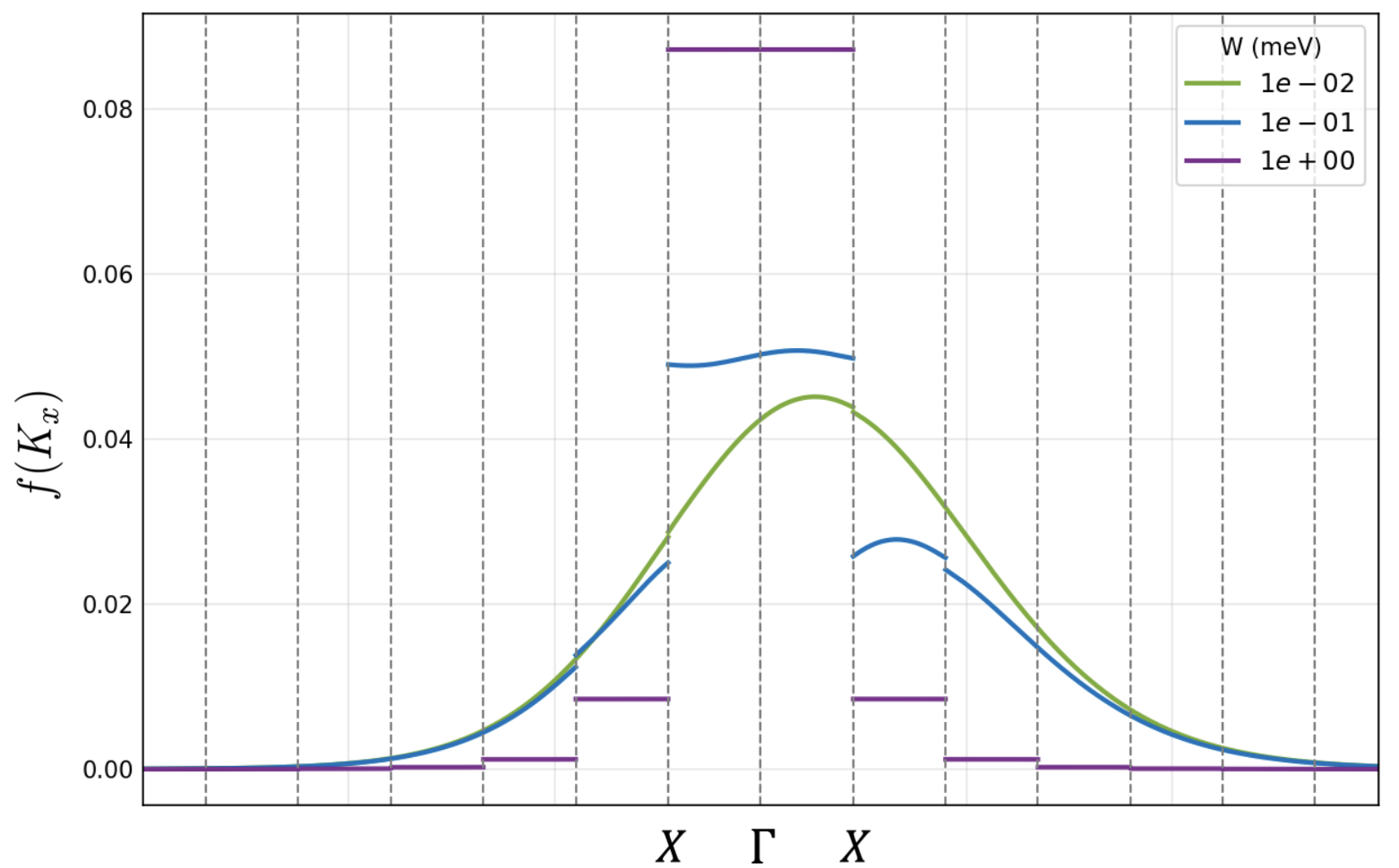
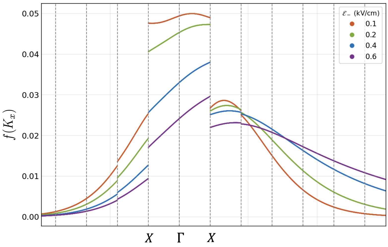
With this information, we can compute the nonequilibrium Boltzmann distribution function and the resulting counterflow conductivity. Typical results for are presented in Fig. 5 in the extended zone scheme for fixed , for different potential strengths [panel (a)] and for different values of [panel (b)] for a system at temperature K and magnetic field T. As is evident in Fig. 5 (a), for meV the distribution functions are nearly identical to that of , indicating that the periodic potential has little effect on the exciton distribution below this potential scale. As increases above this value, visible jumps open at the avoided crossings located at and , and the exciton population increasingly favors the lower over the higher bands, signaling a crossover towards a single-band regime, in which higher bands contribute little to the exciton flow. Moreover, for meV and above, the distribution within each band becomes essentially independent of (for fixed ), so that even highly occupied bands contribute little to the overall counterflow conductivity. This leads to significant suppression of (see below).
The flattening of the distribution function as increases has a direct physical origin in the band structure itself. The periodic potential in Eq. (6) opens increasingly large gaps at the avoided crossings and simultaneously flattens the dispersions of the lowest energy bands (see Fig. 4). The large gaps effectively confine the excitons to single bands, and their lack of energetic dispersion effectively makes all momenta equivalent from the perspective of the equations of motion, resulting in the nearly uniform occupation within a band.
By contrast, raising from small values tends to reduce the effects of gaps in the spectrum. This is illustrated in Fig. 5 (b), where one sees the jumps in the distribution tending to close as increases. Since the total exciton number density is conserved, the lowest band becomes progressively depleted as excitons are driven into higher bands via Landau-Zener tunneling. Here the underlying physics is the increasing probability of interband tunneling as the slew rate increases. In addition, the distribution overall becomes increasingly asymmetric, in a manner reminiscent of the non-equilibrium Boltzmann distribution for electrons in a strong driving field [63].


Fig. 6 illustrates typical results for that result from our numerical computations of the QGD and the non-equilibrium Boltzmann distribution. Panel (a) shows results from Eq. (9) as a function of both and for , , , , , , and . Several features are notable. As , approaches , recovering the results expected for a uniform system, as expected. As increases, the crossover from a dispersive to a flat-band regime and the relatively larger occupation of the lowest band, tends to suppress . This may be understood as a reflection of the suppressed magnitudes that accompanies the energetic flattening of the lowest energy bands. By contrast, increasing while keeping fixed tends to increase the magnitude of . The increased Landau-Zener tunneling and resulting enhancement of higher band occupation brings in the somewhat greater slopes in the QGD evident in Fig. 2(a) as one moves to higher energies, which tends to increase the magnitude of (see Eq. (9).)
Fig. 6 (b) shows as a function of and at fixed meV. Increasing the dielectric constant decreases the electron-hole interaction relative to other energy scales in the problem, effectively weakening the effect of their correlated positions. Several features are notable. (i) Increasing has an effect analogous to increasing : it flattens the QGD at small momentum (see Fig. 7 in Appendix A); however, (ii) as increases, more bands become occupied since the reduced electron-hole binding energy lowers the energy cost of populating higher bands. For the parameters associated with Fig. 6 (b), this effect is larger than (i) above, leading to a net increase in the magnitude of the counterflow conductivity. (iii) As increases at fixed , the Landau-Zener tunneling drives the excitons into higher bands and the magnitude of grows, as was the case in Fig. 6 (a).
IV Summary and Discussion
Excitons generically may be characterized by a quantum geometric dipole, an internal polarization that is tied to the structure of the exciton Hilbert space. In this work we have developed a theory of counterflow conductivity in a system of interlayer excitons, with the goal of identifying features that provide information on this QGD. As a basic example, we have focused on a system of interlayer magnetoexcitons in a strong magnetic field and in a unidirectional periodic potential, inducing a simple exciton band structure. To model transport we developed a semiclassical theory using a Boltzmann distribution function that takes into account both the multiband structure and the Landau-Zener tunneling that may occur between bands in a driven system. Our modeling demonstrates that broad features of the QGD may be inferred from the behavior of , in particular a tendency to be suppressed in the lowest-energy bands when the periodic potential is sufficiently large, and a tendency to be enhanced at relatively high energies. In this way, counterflow conductivity offers a window on the internal quantum geometric structure of excitons.
Not all features of the QGD are captured in a clear way by . Most prominent are the sharp spikes as a function of at the avoided crossings (see Fig. 2). For most bands, these features occupy a very small region of momentum space relative to the full Brillouin zone, in practice yielding only a small contribution to Eq. (9). Better probes of these features could involve co-flow electrical conductivity, which directly probes relative motion of the electrons and holes. A particularly interesting quantity in this context could be frequency-dependent noise [63], which would capture the swift turnaround of the QGD as it passes through an avoided crossing as a high-frequency component. Related to this, one might consider whether high-frequency radiation could be detected as excitons move through the band structure and their dipole moments oscillate. The sharp changes in QGD would be expected to lead to high harmonics of the Bloch oscillation frequency [64] associated with motion through the band structure.
Our model does not include the possibility of generation and recombination of excitons, as well any inhomogeneity in the exciton density in real space. For this reason, the analysis applies most directly to systems in which electron and hole carriers are injected by contacts in the separate layers, and relax into exciton states through inelastic scattering processes. Generalizations of what we have done could incorporate regions of inhomogeneous exciton density, as well as the impact of effectively unbound carriers near contact regions. This would involve generalizing our Boltzmann approach to model non-trivial real-space distributions. Incorporation of generation and recombination would also allow more direct modeling of geometries in which the excitons are generated by laser excitation.
The platform we have considered includes only (magneto-)excitons as current carriers in the two layers. The most directly applicable platforms for such situations would be double layers in which one layer is doped into an electron-like Landau level, and the other into a hole-like Landau level. In principle, graphene and TMD materials could offer such environments. By contrast, one can consider quantum Hall bilayers of total filling factor 1, with a bias such that one layer hosts a nearly filled Landau level with a small density of missing electrons, while the other layer hosts the depleted electrons. With such strong biases, the system is not expected to Bose condense [37]; however, it is quite interesting to consider how Bose condensation would affect the behavior of the system. In addition, a fuller analysis of the bilayer quantum Hall system would require incorporation of the “exciton vacuum” – a filled Landau level – into the computation of
Finally, our choice of excitons in a strong magnetic field as a platform for QGD effects in exciton transport was made because of the relative simplicity it allows in computing the exciton bands and their associated QGD’s. Other platforms are also relevant, particularly excitons in moiré lattice systems which can host relatively large QGD’s [45]. In addition to offering a rich and tunable environment for excitons, the nature of these lattices will likely host behaviors stemming from their two-dimensionality which are not present in our simple unidirectional lattice system. Moreover, it will be interesting to examine whether topological indices may be present in the exciton band structures that impact transport in either the one- or two-dimensional platforms. We leave these questions for future work.
V Acknowledgements
H.A.F. and F.I.M. would like to thank Kaijie Yang and P. Myles Eugenio for comments and discussions. Computational work was supported in part by the Lilly Endowment, Inc., through its support for the Indiana University Pervasive Technology Institute. This work was supported by the NSF through Grant No. DMR-2531425, and by the IU Research Emerging Frontiers program. L.B. acknowledges financial support from the Ministerio de Ciencia e Innovación through the grant PID22024-161156NB-I00. L.B. also acknowledges Severo Ochoa Centres of Excellence program through Grant CEX2024-001445-S.
Appendix A Exciton Band Structure and Multiband QGD
In this Appendix, we provide details on the construction of the exciton band structure and the band-projected QGD in the presence of the one-dimensional periodic potential defined in Eq. (6). In the absence of the periodic potential, exciton states are labeled by the total exciton momentum and take the form
| (23) |
where and are the single-particle wavefunctions provided in Ref. [24] corresponding to the hole and electron residing in Landau levels and respectively, is the magnetic length, and are expansion coefficients, determined by the two-body eigenvalue equation. We work in the strong field limit, where both the electron and hole reside in the lowest Landau level (LLL).
The unperturbed magnetoexciton energy in the LLL is given by [62]
| (24) |
where is a Bessel function of the first kind, is the electron charge, is the interlayer separation, and is the dielectric constant. This expression reflects the Coulomb binding energy of the electron-hole pair in the lowest Landau level, which decreases monotonically in magnitude as increases and asymptotically approaches zero at large , reflecting the vanishing of the binding energy as the pair separation grows [41].
In the presence of the one-dimensional periodic potential
| (25) |
where , the exciton Hamiltonian acquires off-diagonal matrix elements that mix states at momenta and . The matrix elements of the periodic potential between unperturbed exciton states are
| (26) |
The Hamiltonian takes a tridiagonal form in the basis of momentum states. We seek the exciton band structure by constructing the variational wavefunction for the band as an expansion over unperturbed states shifted by reciprocal lattice vectors:
| (27) |
where is a cutoff band retained in the expansion and the coefficients are determined variationally by minimizing the energy . This leads to the eigenvalue equation
| (28) |
where the Hamiltonian matrix elements are
| (29) |
The matrix is thus an tridiagonal Hermitian matrix with , which we diagonalize numerically to obtain the band energies and the expansion coefficients for each band and momentum in the first Brillouin zone.
Our interest is in the evolution of the quantum geometric dipole (QGD) in the presence of a periodic potential as the exciton traverses the Brillouin zone. In this Appendix, we follow closely Ref. [24] in order to derive the band-projected QGD in the presence of a unidirectional periodic potential for the general multiband case. We define the band-projected cell-periodic functions constructed from Eq. (27)
| (30) |
where and label the hole and electron constituents of the exciton, respectively. These allow us to define the band-projected Berry connections for each constituent in accordance with Ref. [24]:
| (31) |
with the band-projected QGD formally defined as their difference
| (32) |
To compute this, we introduce the generalized overlap matrix element
| (33) |
which allows us to express the difference of the Berry’s connections as
| (34) |
Substituting Eq. (30) into Eq. (33), we find
| (35) |
| (36) |
where and are the overlaps analogous to Eq. 33 for the uniform system (see Ref. [24]), and cross terms between different values of vanish because states at momenta and with are orthogonal when . Taking the gradient of the difference of the overlaps with respect to , and substituting into Eq. (34), we obtain
| (37) |
Recognizing that the quantity inside the sum is precisely the QGD of a uniform magnetoexciton evaluated at momentum [24], we arrive at the central result of this Appendix,
| (38) |
where is the QGD of a magnetoexciton for a uniform system [24, 25].
Results for the QGD at different values of are presented in the main text. To conclude this Appendix, we illustrate the effect of the dielectric constant on the band-projected QGD. Fig. 7 shows at fixed for several values of . As increases, the Coulomb interaction between the electron and hole is increasingly screened, which modifies the unperturbed magnetoexciton dispersion and consequently the expansion coefficients . The result is a suppression and flattening of the band-projected QGD at small momentum, reflecting the reduced electron-hole binding and the redistribution of spectral weight among the shifted momentum states . This behavior is analogous to increasing in that both suppress the QGD gradient that enters the counterflow conductivity Eq. (9). Competing with this, for high bands the QGD grows in magnitude with increasing faster than would be expected based purely on zone-folding, in a way analogous to what happens with increasing at fixed : the contribution from states of higher momenta to the exciton wavefunctions tends to increasingly outweigh those of lower momenta as the band index (and exciton energy) increases, giving extra weight to contributions with larger QGD.

Appendix B Counterflow Conductivity
In this Appendix, we provide details of the derivation of the counterflow conductivity tensor starting from the semiclassical equations of motion. This is constructed from the exciton number current, which induces electric currents in opposite directions in the two layers, leading to an electric counterflow current
| (39) |
where is the velocity of an exciton center-of-mass coordinate in band , whose evolution is given by the equations of motion Eq. (4), and is the nonequilibrium distribution function obtained from the Boltzmann equation described in the main text. Since we are interested in the contribution of the QGD to transport, the form of Eq. (4) suggest we should consider the deviation of the current from its value in the absence of the symmetric field ,
| (40) |
Note that the distribution function depends on but not on , since the antisymmetric field drives the exciton momentum while the symmetric field couples only to the QGD. This separation is what makes a linear response to .
Decomposing Eq. (40) into component form, valid whether is static or dynamic,
| (41) |
Identifying the quantity in braces with the conductivity tensor via , we arrive at the general expression for the counterflow conductivity,
| (42) |
as displayed in the main text. It shows that the counterflow conductivity is determined by two ingredients: the nonequilibrium distribution function , which encodes the response of the exciton population to , and the gradient of the band-projected QGD , which encodes the quantum geometric structure of the exciton band.
In what follows, we evaluate each component of using the explicit form of the band-projected QGD derived in Appendix A. Recalling that , the two components of the band-projected QGD are
| (43) |
and
| (44) |
where we used the normalization condition . Note that the -component is independent of both the band index and , while the -component retains a nontrivial and dependence through the weighted sum .
From Eq. (43), is independent of and , and its derivative with respect to is simply
| (45) |
Substituting into Eq. (42), one obtains
| (46) |
where we used , the total exciton number density [65]. This recovers Eq. (11) of the main text, and holds for any distribution function , independently of the periodic potential strength or the driving field .
For , we require . Differentiating Eq. (44) with respect to yields
| (47) |
which depends nontrivially on through the -dependence of the expansion coefficients . These are determined by the diagonalization of the tridiagonal Hamiltonian matrix described in Appendix A and must be evaluated numerically. Substituting into Eq. (42) yields
| (48) |
In our computations we evaluate this numerically using the band-projected QGD (Appendix A) and the nonequilibrium distribution function obtained from the Boltzmann equation as described in in the main text.
We now demonstrate that vanishes exactly. From Eq. (42) we have
| (49) |
Eq. (43),tells us that is independent of for all bands . Therefore,
| (50) |
from which it immediately follows that
Finally we consider , which requires . In the absence of the periodic potential, this quantity vanishes identically because the QGD in this situation is purely transverse. In the presence of the periodic potential, differentiating Eq. (44) with respect to yields
| (51) |
There is a weak -dependence in the eigenvector coefficients , making small but generically nonzero. For example, typical values of are less than . For this reason we focus on and in the main text.
References
- Geim and Grigorieva [2013] A. K. Geim and I. V. Grigorieva, Nature 499, 419 (2013).
- Novoselov et al. [2016] K. S. Novoselov, A. Mishchenko, A. Carvalho, and A. H. Castro Neto, Science 353, aac9439 (2016).
- Novoselov et al. [2005] K. S. Novoselov, D. Jiang, F. Schedin, T. Booth, V. Khotkevich, S. Morozov, and A. K. Geim, Proceedings of the National Academy of Sciences 102, 10451 (2005).
- Liu et al. [2016] Y. Liu, N. O. Weiss, X. Duan, H.-C. Cheng, Y. Huang, and X. Duan, Nature Reviews Materials 1, 16042 (2016).
- Cao et al. [2018a] Y. Cao et al., Nature 556, 80 (2018a).
- Cao et al. [2018b] Y. Cao et al., Nature 556, 43 (2018b).
- Huang et al. [2017] B. Huang et al., Nature 546, 270 (2017).
- Gong et al. [2017] C. Gong et al., Nature 546, 265 (2017).
- Cai et al. [2023] J. Cai et al., Nature 622, 63 (2023).
- Park et al. [2023] H. Park, J. Cai, E. Anderson, Y. Zhang, J. Zhu, X. Liu, C. Wang, W. Holtzmann, C. Hu, Z. Liu, et al., Nature 622, 74 (2023).
- Zeng et al. [2023] Y. Zeng et al., Nature 622, 69 (2023).
- Kennes et al. [2021] D. M. Kennes et al., Nature Physics 17, 155 (2021).
- Gibertini et al. [2019] M. Gibertini et al., Nature Nanotechnology 14, 408 (2019).
- Rohlfing and Louie [2000] M. Rohlfing and S. G. Louie, Physical Review B 62, 4927 (2000).
- Wang et al. [2018] G. Wang, A. Chernikov, M. M. Glazov, T. F. Heinz, X. Marie, T. Amand, and B. Urbaszek, Reviews of Modern Physics 90, 021001 (2018).
- Wannier [1937] G. H. Wannier, Physical Review 52, 191 (1937).
- Knox [1963] R. Knox, Press, NY (1963).
- Chernikov et al. [2014] A. Chernikov, T. C. Berkelbach, H. M. Hill, A. Rigosi, Y. Li, B. Aslan, D. R. Reichman, M. S. Hybertsen, and T. F. Heinz, Physical review letters 113, 076802 (2014).
- Mueller and Malic [2018] T. Mueller and E. Malic, npj 2D Materials and Applications 2, 29 (2018).
- Srivastava and Imamoğlu [2015] A. Srivastava and A. Imamoğlu, Physical Review Letters 115, 166802 (2015).
- Zhou et al. [2015] J. Zhou, W.-Y. Shan, W. Yao, and D. Xiao, Physical Review Letters 115, 166803 (2015).
- Yao and Niu [2008] W. Yao and Q. Niu, Physical Review Letters 101, 106401 (2008).
- Kwan et al. [2021] Y. H. Kwan, Y. Hu, S. H. Simon, and S. A. Parameswaran, Physical Review Letters 126, 137601 (2021).
- Cao et al. [2021a] J. Cao, H. A. Fertig, and L. Brey, Physical Review B 103, 115422 (2021a).
- Fertig and Brey [2025] H. A. Fertig and L. Brey, Physical Review B 111, 035158 (2025).
- Chaudhary et al. [2021] S. Chaudhary, C. Knapp, and G. Refael, Physical Review B 103, 165119 (2021).
- Paiva et al. [2024] C. Paiva, T. Holder, and R. Ilan, arXiv preprint arXiv:2408.10300 (2024).
- Davenport et al. [2026] H. Davenport, J. Knolle, and F. Schindler, Physical Review B 113, 045125 (2026).
- Xie et al. [2024] H.-Y. Xie, P. Ghaemi, M. Mitrano, and B. Uchoa, Proceedings of the National Academy of Sciences 121, e2401644121 (2024).
- Lozano et al. [2025] M. Lozano, H.-Y. Xie, and B. Uchoa, arXiv:2509.03601 (2025).
- Chen et al. [2025] L. Chen, S. A. A. Ghorashi, J. Cano, and V. Crépel, Quantum-geometric dipole: a topological boost to flavor ferromagnetism in flat bands (2025).
- Cao et al. [2021b] J. Cao, H. Fertig, and L. Brey, Physical review letters 127, 196403 (2021b).
- Cao et al. [2022] J. Cao, H. Fertig, and L. Brey, Physical Review B 106, 165125 (2022).
- Jauregui et al. [2019] L. A. Jauregui, A. Y. Joe, K. Pistunova, D. S. Wild, A. A. High, Y. Zhou, G. Scuri, K. De Greve, A. Sushko, C.-H. Yu, T. Taniguchi, K. Watanabe, D. J. Needleman, M. D. Lukin, H. Park, and P. Kim, Science 366, 870 (2019).
- Rivera et al. [2015] P. Rivera et al., Nature Communications 6, 6242 (2015).
- Eisenstein et al. [1990] J. Eisenstein, L. Pfeiffer, and K. West, Applied physics letters 57, 2324 (1990).
- Eisenstein and MacDonald [2004] J. P. Eisenstein and A. H. MacDonald, Nature 432, 691 (2004).
- Liu et al. [2017] X. Liu, K. Watanabe, T. Taniguchi, B. I. Halperin, and P. Kim, Nature Physics 13, 746 (2017).
- Li et al. [2017] J. I. A. Li, T. Taniguchi, K. Watanabe, J. Hone, and C. R. Dean, Nature Physics 13, 751 (2017).
- Wang et al. [2019] Z. Wang, D. A. Rhodes, K. Watanabe, T. Taniguchi, J. C. Hone, J. Shan, and K. F. Mak, Nature 574, 76 (2019).
- Kallin and Halperin [1984] C. Kallin and B. I. Halperin, Physical Review B 30, 5655 (1984).
- Lerner and Lozovik [1980] I. V. Lerner and Y. E. Lozovik, Sov. Phys. JETP 51, 588 (1980).
- Bychkov et al. [1996] Y. A. Bychkov, S. V. Iordanskii, and G. M. Éliashberg, in World Scientific Series in 20th Century Physics, Vol. 11 (WORLD SCIENTIFIC, 1996) pp. 190–193.
- Kozin et al. [2021] V. Kozin, V. Shabashov, A. Kavokin, and I. Shelykh, Physical Review Letters 126, 036801 (2021).
- Yang et al. [2026] K. Yang, H. Zheng, X. Xu, D. Xiao, and T. Cao, arXiv preprint arXiv:2604.12295 (2026).
- Xiao et al. [2010] D. Xiao, M.-C. Chang, and Q. Niu, Reviews of modern physics 82, 1959 (2010).
- Nagaosa et al. [2010] N. Nagaosa, J. Sinova, S. Onoda, A. H. MacDonald, and N. P. Ong, Reviews of modern physics 82, 1539 (2010).
- Xiao et al. [2005] D. Xiao, J. Shi, and Q. Niu, Physical review letters 95, 137204 (2005).
- Sodemann and Fu [2015] I. Sodemann and L. Fu, Physical review letters 115, 216806 (2015).
- Guo et al. [2025] W. Guo, L. Li, Q. Tong, and C. Li, arXiv preprint arXiv:2512.24153 (2025).
- Jauregui and Kim [2017] L. A. Jauregui and P. Kim, Nature Materials 16, 1169 (2017).
- Kovalev and Savenko [2019] V. Kovalev and I. Savenko, Physical Review B 100, 121405 (2019).
- De Beule and Mele [2023] C. De Beule and E. Mele, Physical Review Letters 131, 196603 (2023).
- Finck et al. [2011] A. D. K. Finck, J. P. Eisenstein, L. N. Pfeiffer, and K. W. West, Physical Review Letters 106, 236807 (2011).
- Su and MacDonald [2008] J.-J. Su and A. H. MacDonald, Nature Physics 4, 799 (2008).
- Kellogg et al. [2002] M. Kellogg, I. Spielman, J. Eisenstein, L. Pfeiffer, and K. West, Physical review letters 88, 126804 (2002).
- Kellogg et al. [2004] M. Kellogg, J. Eisenstein, L. Pfeiffer, and K. West, Physical review letters 93, 036801 (2004).
- Tutuc et al. [2004] E. Tutuc, M. Shayegan, and D. Huse, Physical review letters 93, 036802 (2004).
- Wiersma et al. [2004] R. Wiersma, J. Lok, S. Kraus, W. Dietsche, K. Von Klitzing, D. Schuh, M. Bichler, H.-P. Tranitz, and W. Wegscheider, Physical review letters 93, 266805 (2004).
- Yan et al. [2009] J.-Y. Yan, S. Duan, W. Zhang, and X.-G. Zhao, Physical Review A—Atomic, Molecular, and Optical Physics 79, 053613 (2009).
- Rubbmark et al. [1981] J. R. Rubbmark, M. M. Kash, M. G. Littman, and D. Kleppner, Physical Review A 23, 3107 (1981).
- Fertig [1989] H. Fertig, Physical Review B 40, 1087 (1989).
- Stanton and Wilkins [1987] C. J. Stanton and J. W. Wilkins, Physical Review B 35, 9722 (1987).
- Fahimniya et al. [2021] A. Fahimniya, Z. Dong, E. I. Kiselev, and L. Levitov, Physical Review Letters 126, 256803 (2021).
- Girvin and Yang [2019] S. M. Girvin and K. Yang, Modern condensed matter physics (Cambridge University Press, 2019).
