跳到论文正文
W Papers独立论文阅读器 arXiv:2605.21296 论文正文 计算阅读时间 · 0%
引用这篇论文根据当前论文元数据生成,正式投稿前建议核对。


License: arXiv.org perpetual non-exclusive license
arXiv:2605.21296v1 [math.AP] 20 May 2026

Well-posedness and asymptotic limits for a degenerate Keller–Segel system with volume filling

Noah Geltner Institute of Analysis and Scientific Computing, TU Wien, Wiedner Hauptstraße 8–10, 1040 Wien, Austria noah.geltner@tuwien.ac.at , Ansgar Jüngel Institute of Analysis and Scientific Computing, TU Wien, Wiedner Hauptstraße 8–10, 1040 Wien, Austria juengel@tuwien.ac.at and Mingyue Zhang Institute of Analysis and Scientific Computing, TU Wien, Wiedner Hauptstraße 8–10, 1040 Wien, Austria mingyue.zhang@tuwien.ac.at
Abstract.

A class of parabolic–parabolic Keller–Segel systems with degenerate diffusion and volume filling is studied in a bounded domain subject to no-flux boundary conditions. The equations are derived from a multiphase fluid model. The interplay between nonlinear diffusion and density saturation leads to a rich variety of behaviors across different parameter regimes. We establish the existence of global weak solutions, a weak–strong uniqueness result, the exponential convergence to the homogeneous steady state, pattern formation in one spatial dimension, as well as the parabolic–elliptic and vanishing diffusion limits. The analysis relies on a priori estimates derived from suitable entropy functionals. Pattern formation is demonstrated by reducing the system to a first-order equation and conducting a detailed analysis of the resulting nonlinearity. Numerical simulations from a one-dimensional finite-volume scheme illustrate the asymptotic regimes.

Key words and phrases:
Keller–Segel equations, existence of weak solutions, weak–strong uniqueness, steady states, pattern formation, parabolic–elliptic limit, vanishing diffusion limit.
2000 Mathematics Subject Classification:
35K51, 35K65, 35B36, 35Q92, 92C17.
The authors acknowledge partial support from the Austrian Science Fund (FWF), grant 10.55776/PAT2687825, and from the Austrian Federal Ministry for Women, Science and Research and implemented by ÖAD, project MultHeFlo. This work has received funding from the European Research Council (ERC) under the European Union’s Horizon 2020 research and innovation programme, ERC Advanced Grant NEUROMORPH, no. 101018153. For open-access purposes, the authors have applied a CC BY public copyright license to any author-accepted manuscript version arising from this submission.

1. Introduction

The Keller–Segel equations provide a fundamental mathematical framework for describing how populations of cells sense and collectively migrate along chemical signals [16]. While the classical Keller–Segel model assumes linear diffusion and constant sensitivity, generalized models account for finite-speed propagation or the prevention of overcrowding. Mathematically, this can be modeled by degenerate diffusion [6, 23] or a modification of the chemotactic sensitivity which diminishes as the cell density approaches a maximal packing threshold [8, 21]. The resulting system, derived from a multiphase fluid model and studied here for the first time, combines degenerate diffusion with nonlinear, density-limited chemotactic drift, yielding a rich mathematical structure: It prevents unphysical blowup present in classical Keller–Segel models, while still capturing pattern formation, aggregation, and saturation phenomena observed in real biological systems. Moreover, depending on the nonlinear diffusion, we distinguish parameter regimes in which pattern formation either emerges or is inhibited.

The Keller–Segel equations for the cell density ρ​(t,x)\rho(t,x) and the concentration of the chemoattractant c​(t,x)c(t,x) are given by

(1) ∂tρ\displaystyle\partial_{t}\rho =div⁡((1−ρ)​ρm−1​∇ρ−χ​ρ​(1−ρ)​∇c),\displaystyle=\operatorname{div}\big((1-\rho)\rho^{m-1}\nabla\rho-\chi\rho(1-\rho)\nabla c\big),
(2) τ​∂tc\displaystyle\tau\partial_{t}c =η​Δ​c−c+ρin ​Ω,t>0,\displaystyle=\eta\Delta c-c+\rho\quad\mbox{in }\Omega,\ t>0,

supplemented with the initial and no-flux boundary conditions

(3) ρ​(0)=ρ0,c​(0)=c0,in ​Ω,\displaystyle\rho(0)=\rho^{0},\quad c(0)=c^{0},\quad\mbox{in }\Omega,
(1−ρ)​ρm−1​∇ρ⋅ν=∇c⋅ν=0on ​∂Ω,t>0,\displaystyle(1-\rho)\rho^{m-1}\nabla\rho\cdot\nu=\nabla c\cdot\nu=0\quad\mbox{on }\partial\Omega,\ t>0,

where 0≤ρ0,c0≤10\leq\rho^{0},c^{0}\leq 1 in Ω\Omega. The biological parameters are the degeneracy exponent m>1m>1, the chemotactic sensitivity χ\chi, the characteristic time τ\tau, and the chemical diffusion rate η>0\eta>0.

Both diffusion and drift in (1) vanish as the cell density approaches a maximal packing threshold. The exponent m>1m>1, which expresses slow diffusion, plays a crucial role in pattern formation: For instance, steady states (more precisely: equilibrium solutions) are positive for m=1m=1, whereas for m>1m>1, they may vanish on subsets of the domain.

Our model can be derived formally from mass and momentum balance equations in the multiphase approach by assuming that the total interaction force is given by interphase, chemotactic, and drag forces; see Appendix A. Equations (1)–(2) can also be interpreted as the formal gradient flow

∂tρ=div⁡(M​(ρ)​∇δ​Eδ​ρ),χ​τ​∂tc=−δ​Eδ​c,\displaystyle\partial_{t}\rho=\operatorname{div}\bigg(M(\rho)\nabla\frac{\delta E}{\delta\rho}\bigg),\quad\chi\tau\partial_{t}c=-\frac{\delta E}{\delta c},
whereE​(ρ,c)=∫Ω(ρmm​(m−1)+χ2​(η​|∇c|2+c2)−χ​ρ​c)​𝑑x\displaystyle\mbox{where}\quad E(\rho,c)=\int_{\Omega}\bigg(\frac{\rho^{m}}{m(m-1)}+\frac{\chi}{2}(\eta|\nabla c|^{2}+c^{2})-\chi\rho c\bigg)dx

is the energy and the mobility reads as M​(ρ)=ρ​(1−ρ)M(\rho)=\rho(1-\rho), used in [6]. Such a relation also holds in the case m=1m=1, with ρm/(m​(m−1))\rho^{m}/(m(m-1)) replaced by ρ​(log⁡ρ−1)\rho(\log\rho-1).

The mathematical modeling of chemotaxis phenomena dates back to the pioneering works of Patlak in the 1950s [22] and Keller and Segel in the 1970s [16]. Since then, the body of mathematical literature on the Keller–Segel equations has grown extensively. We highlight only some contributions concerning degenerate and volume-filling models. For notational convenience, we write the general Keller–Segel equations as

(4) ∂tρ=div⁡(a​(ρ)​∇ρ−b​(ρ)​∇c),τ​∂tc=η​Δ​c−c+ρ,\displaystyle\partial_{t}\rho=\operatorname{div}\big(a(\rho)\nabla\rho-b(\rho)\nabla c\big),\quad\tau\partial_{t}c=\eta\Delta c-c+\rho,

where aa and bb are nonlinear functions.

Degenerate Keller–Segel equations with a​(ρ)=ρm−1a(\rho)=\rho^{m-1} (m>1m>1) and b​(ρ)=χ​ρb(\rho)=\chi\rho exhibit a finite speed of propagation of the cell movement, which seems to be a realistic cell behavior. The existence of global weak solutions for m>3−4/dm>3-4/d was proved in [17] and later improved to the optimal range m>2−2/dm>2-2/d [24]. The convergence to possibly nonconstant steady states for m≥2m\geq 2 and to the constant steady state for m=2m=2 was proved in [14]. A complete phase transition diagram for the one-dimensional model with m=2m=2 was given in [8].

Hillen and Painter [21] derived a volume-filling Keller–Segel system from a lattice model with the functions a​(ρ)=q​(ρ)−ρ​q′​(ρ)a(\rho)=q(\rho)-\rho q^{\prime}(\rho) and b​(ρ)=ρ​q​(ρ)b(\rho)=\rho q(\rho), where qq is nonnegative and satisfies q​(1)=0q(1)=0. The simplest choice q​(ρ)=1−ρq(\rho)=1-\rho leads to a​(ρ)=1a(\rho)=1 (analyzed in [12]); thus, this class of models is different from our system. Conditions on a​(ρ)a(\rho) and b​(ρ)b(\rho) such that the solutions do not blow up were given in [6, 7] for the elliptic case τ=0\tau=0 and in [11] for the parabolic case τ>0\tau>0. In [25], pattern formation of the parabolic model τ>0\tau>0 was investigated. For a comprehensive review of volume-filling chemotaxis models, we refer the reader to [27].

Also combined degenerate and volume-filling Keller–Segel equations have been studied in the literature. The model of Hillen and Painter with the choice q​(ρ)=(1−ρ)rq(\rho)=(1-\rho)^{r} with r>1r>1 was investigated in [26], and general functions qq have been considered in [18]. Bendahmane and co-workers [4] proved the existence of Hölder continuous solutions to (4) with a​(0)=a​(1)=0a(0)=a(1)=0 and b​(1)=0b(1)=0. Although these properties are satisfied in our model, the other assumptions imposed in [4] do not hold in our situation. Solutions to (4) blow up in finite time if the nonlinear chemosensitivity is strong enough and an adequate relation between nonlinear diffusion and chemosensitivity holds [9]. Pattern formation for a​(ρ)=ρm−1a(\rho)=\rho^{m-1} and b​(ρ)=χ​ρ​(1−ρ)b(\rho)=\chi\rho(1-\rho) was shown in [23] when m>2m>2, while the steady state for m≤2m\leq 2 is shown to be unique and constant. Notice that in our model, the function a​(ρ)=(1−ρ)​ρm−1a(\rho)=(1-\rho)\rho^{m-1} features a stronger nonlinearity, which complicates the analysis. Finally, we mention the reviews [2, 3], which provide an overview of the various variants of the Keller–Segel equations.

In this paper, we prove the existence of global weak solutions to (1)–(3), investigate the weak–strong uniqueness, study pattern formation for m>2m>2, study the long-time behavior for m≤2m\leq 2, as well as perform the parabolic–elliptic limit τ→0\tau\to 0 and the vanishing diffusion limit η→0\eta\to 0. In the following, we make precise our main results.

Let Ω⊂ℝd\Omega\subset{\mathbb{R}}^{d} (d≥1d\geq 1) be a bounded domain with boundary ∂Ω∈C1,1\partial\Omega\in C^{1,1} and let χ\chi, τ\tau, η>0\eta>0. The initial data satisfies ρ0∈Lm​(Ω)\rho^{0}\in L^{m}(\Omega), c0∈H1​(Ω)c^{0}\in H^{1}(\Omega), and 0≤ρ00\leq\rho^{0}, c0≤1c^{0}\leq 1 in Ω\Omega. We set ΩT=(0,T)×Ω\Omega_{T}=(0,T)\times\Omega for T>0T>0. Our first result is the existence of global weak solutions.

Theorem 1 (Existence of weak solutions).

Let m≥1m\geq 1 and set f​(ρ)=ρm/m−ρm+1/(m+1)f(\rho)=\rho^{m}/m-\rho^{m+1}/(m+1). Then there exists a weak solution (ρ,c)(\rho,c) to (1)–(3) on [0,∞)[0,\infty) satisfying 0≤ρ,c≤10\leq\rho,\,c\leq 1 a.e. in [0,∞)×Ω[0,\infty)\times\Omega,

f​(ρ)∈L2​(0,T;H1​(Ω)),c∈L∞​(0,T;H1​(Ω)),\displaystyle f(\rho)\in L^{2}(0,T;H^{1}(\Omega)),\quad c\in L^{\infty}(0,T;H^{1}(\Omega)),
∂tρ∈L2​(0,T;H1​(Ω)′),∂tc,Δ​c∈L2​(ΩT)\displaystyle\partial_{t}\rho\in L^{2}(0,T;H^{1}(\Omega)^{\prime}),\quad\partial_{t}c,\,\Delta c\in L^{2}(\Omega_{T})

for any T>0T>0, and (ρ,c)(\rho,c) satisfies (1)–(2) in the weak sense.

To prove this theorem, we regularize equation (1) by adding the diffusion ε​Δ​ρ\varepsilon\Delta\rho with ε>0\varepsilon>0 to (1) and truncating the nonlinearities. The regularized problem is solved by a fixed-point argument. The approximate entropy inequality yields estimates uniform in ε\varepsilon, which allow for the limit ε→0\varepsilon\to 0 by applying the Aubin–Lions lemma in the version of [20] to the (monotone) function f​(ρ)f(\rho).

The proof of uniqueness of weak solutions to degenerate Keller–Segel systems is very delicate, and we are aware of results mainly for a​(ρ)=ρma(\rho)=\rho^{m} and b​(ρ)=χ​ρb(\rho)=\chi\rho only [15, 17]. A nonlocal sensitivity was considered in [13]. The proof in [10] requires that b′b^{\prime} vanishes at ρ=0\rho=0, which is not the case in our model. Therefore, we prove the (weaker) weak–strong uniqueness property. The aim is to show that a weak solution and a strong solution (if it exists) emanating from the same initial data coincide. Weak–strong uniqueness means that classical solutions are stable within the class of weak solutions.

Theorem 2 (Weak–strong uniqueness).

Let 1<m≤21<m\leq 2, let (ρ,c)(\rho,c) and (ρ¯,c¯)(\bar{\rho},\bar{c}) be two weak solutions to (1)–(3) with the same initial data. Assume that there exists κ∈(0,1)\kappa\in(0,1) such that κ≤ρ¯≤1−κ\kappa\leq\bar{\rho}\leq 1-\kappa in ΩT\Omega_{T} and that ∇ρ¯\nabla\bar{\rho}, ∇c¯∈L∞​(ΩT)\nabla\bar{c}\in L^{\infty}(\Omega_{T}). Furthermore, we suppose that (ρ¯,c¯)(\bar{\rho},\bar{c}) satisfies for all λ>0\lambda>0 the entropy equality

∫Ω\displaystyle\int_{\Omega} (ρ¯​(log⁡ρ¯−1)+(1−ρ¯)​(log⁡(1−ρ¯)−1)+λ2​τ​c2)​d​x|0t\displaystyle\bigg(\bar{\rho}(\log\bar{\rho}-1)+(1-\bar{\rho})(\log(1-\bar{\rho})-1)+\frac{\lambda}{2}\tau c^{2}\bigg)dx\bigg|_{0}^{t}
+∫0t∫Ω(ρ¯m−2​|∇ρ¯|2+λ​(η​|∇c¯|2+c¯2))​𝑑x​𝑑s=∫0t∫Ω(χ​∇c¯⋅∇ρ¯+λ​ρ¯​c¯)​𝑑x​𝑑s.\displaystyle+\int_{0}^{t}\int_{\Omega}\big(\bar{\rho}^{m-2}|\nabla\bar{\rho}|^{2}+\lambda(\eta|\nabla\bar{c}|^{2}+\bar{c}^{2})\big)dxds=\int_{0}^{t}\int_{\Omega}\big(\chi\nabla\bar{c}\cdot\nabla\bar{\rho}+\lambda\bar{\rho}\bar{c}\big)dxds.

Then ρ=ρ¯\rho=\bar{\rho} and c=c¯c=\bar{c} a.e. in ΩT\Omega_{T}.

The proof of the weak–strong uniqueness property is based on the relative entropy

H​(ρ,c|ρ¯,c¯)=∫Ω(ρ​log⁡ρρ¯+(1−ρ)​log⁡1−ρ1−ρ¯+λ2​τ​(c−c¯)2)​𝑑x,\displaystyle H(\rho,c|\bar{\rho},\bar{c})=\int_{\Omega}\bigg(\rho\log\frac{\rho}{\bar{\rho}}+(1-\rho)\log\frac{1-\rho}{1-\bar{\rho}}+\frac{\lambda}{2}\tau(c-\bar{c})^{2}\bigg)dx,

where (ρ,c)(\rho,c) is a weak solution and (ρ¯,c¯)(\bar{\rho},\bar{c}) is a strong solution (i.e. a weak solutions satisfying the regularity stated in Theorem 2) with the same initial data. The aim is to show that there exists C>0C>0 such that

dd​t​H​(ρ,c|ρ¯,c¯)≤C​H​(ρ,c|ρ¯,c¯)for ​t>0,\displaystyle\frac{d}{dt}H(\rho,c|\bar{\rho},\bar{c})\leq CH(\rho,c|\bar{\rho},\bar{c})\quad\mbox{for }t>0,

which implies that H​((ρ,c)​(t)|(ρ¯,c¯)​(t))=0H((\rho,c)(t)|(\bar{\rho},\bar{c})(t))=0 and hence ρ​(t)=ρ¯​(t)\rho(t)=\bar{\rho}(t), c​(t)=c¯​(t)c(t)=\bar{c}(t) for all t>0t>0. The restriction on the parameter mm comes from the different exponents in the diffusion and drift terms of (1) that need to be estimated. The condition κ≤ρ¯≤1−κ\kappa\leq\bar{\rho}\leq 1-\kappa is technical; it ensures that the relative entropy is well defined.

Next, we investigate the steady states and the long-time behavior. More precisely, we consider equilibrium solutions, i.e. stationary solutions with vanishing flux. We show that for 1<m≤21<m\leq 2, the steady state is unique and constant; see Proposition 8. When m>2m>2 and χ\chi is in some range, we prove for the one-dimensional equations that there exist increasing steady states, thus showing pattern formation; see Proposition 9. The proof relies on a reduction of the problem to a first-order equation for cc and a careful analysis of the involved nonlinearities and parameter dependencies. Because of these results, the convergence to the (unique) steady state can only be expected in the case 1<m≤21<m\leq 2.

Theorem 3 (Exponential time decay).

Let 1<m≤21<m\leq 2, χ≤1\chi\leq 1, |Ω|=1|\Omega|=1, M=∫Ωρ0​𝑑x=∫Ωc0​𝑑xM=\int_{\Omega}\rho_{0}dx=\int_{\Omega}c^{0}dx, and let (ρ,c)(\rho,c) be the solution constructed in Theorem 1. Then there exist C>0C>0, depending on (τ,ρ0,c0,Ω,M)(\tau,\rho^{0},c^{0},\Omega,M), and μ>0\mu>0, depending on (η,τ,Ω,M)(\eta,\tau,\Omega,M), such that for all t>0t>0,

‖ρ​(t)−M‖L2​(Ω)+‖c​(t)−M‖H1​(Ω)≤C​e−μ​t.\displaystyle\|\rho(t)-M\|_{L^{2}(\Omega)}+\|c(t)-M\|_{H^{1}(\Omega)}\leq Ce^{-\mu t}.

The proof is based on the relative entropy method, similar as for the weak–strong uniqueness proof, but here for the functional

(5) H1​(ρ,c|M,M)=∫Ω(ρ​log⁡ρM+(1−ρ)​log⁡1−ρ1−M+τ2​|∇c|2)​𝑑x.\displaystyle H_{1}(\rho,c|M,M)=\int_{\Omega}\bigg(\rho\log\frac{\rho}{M}+(1-\rho)\log\frac{1-\rho}{1-M}+\frac{\tau}{2}|\nabla c|^{2}\bigg)dx.

We prove that there exists μ>0\mu>0 such that for t>0t>0,

dd​t​H1​(ρ,c|M,M)+μ​H1​(ρ,c|M,M)≤0,\displaystyle\frac{d}{dt}H_{1}(\rho,c|M,M)+\mu H_{1}(\rho,c|M,M)\leq 0,

implying that H1​((ρ,c)​(t)|M,M)≤H1​(ρ0,c0|M,M)​e−μ​tH_{1}((\rho,c)(t)|M,M)\leq H_{1}(\rho^{0},c^{0}|M,M)e^{-\mu t}. The result then follows from a Taylor expansion of the relative entropy and an L2​(Ω)L^{2}(\Omega)-type estimation for equation (2).

We also prove the limit τ→0\tau\to 0, leading to the parabolic–elliptic model, and the vanishing diffusion limit η→0\eta\to 0.

Theorem 4 (Parabolic–elliptic limit).

Let m>1m>1 and let (ρτ,cτ)(\rho_{\tau},c_{\tau}) be a weak solution to (1)–(3). Then there exists a subsequence (not relabeled) such that, as τ→0\tau\to 0,

ρτ→ρstrongly in ​Lp​(ΩT)​ for all ​p<∞,cτ→cstrongly in ​L2​(0,T;H1​(Ω)),\displaystyle\rho_{\tau}\to\rho\quad\mbox{strongly in }L^{p}(\Omega_{T})\mbox{ for all }p<\infty,\quad c_{\tau}\to c\quad\mbox{strongly in }L^{2}(0,T;H^{1}(\Omega)),

and (ρ,c)(\rho,c) is a weak solution to

(6) ∂tρ=div⁡((1−ρ)​ρm−1​∇ρ−χ​ρ​(1−ρ)​∇c),0=−η​Δ​c−c+ρin ​Ω,t>0,\displaystyle\partial_{t}\rho=\operatorname{div}\big((1-\rho)\rho^{m-1}\nabla\rho-\chi\rho(1-\rho)\nabla c\big),\quad 0=-\eta\Delta c-c+\rho\quad\mbox{in }\Omega,\ t>0,

with the initial and boundary conditions (3).

Theorem 5 (Vanishing diffusion limit).

Let 1<m≤21<m\leq 2 and let (ρη,cη)(\rho_{\eta},c_{\eta}) be a weak solution to (1)–(3). Then there exists a subsequence (not relabeled) such that, as η→0\eta\to 0,

ρη→ρ,cη→cstrongly in ​L2​(ΩT),\displaystyle\rho_{\eta}\to\rho,\quad c_{\eta}\to c\quad\mbox{strongly in }L^{2}(\Omega_{T}),

and (ρ,c)(\rho,c) is a weak solution to

(7) ∂tρ=div⁡((1−ρ)​ρm−1​∇ρ−χ​ρ​(1−ρ)​∇c),∂tc=−c+ρin ​Ω,t>0,\displaystyle\partial_{t}\rho=\operatorname{div}\big((1-\rho)\rho^{m-1}\nabla\rho-\chi\rho(1-\rho)\nabla c\big),\quad\partial_{t}c=-c+\rho\quad\mbox{in }\Omega,\ t>0,

with the initial and boundary conditions (3).

If the limit equations are uniquely solvable, we recover the convergence for the whole sequence. To prove Theorems 4 and 5, we derive uniform estimates from entropy functionals. For the limit τ→0\tau\to 0, we use

(8) Fτ​(ρ,c)=∫Ω(ρ​(log⁡ρ−1)+(1−ρ)​(log⁡(1−ρ)−1)+χ​τ​ρ​c)​𝑑x,\displaystyle F_{\tau}(\rho,c)=\int_{\Omega}\big(\rho(\log\rho-1)+(1-\rho)(\log(1-\rho)-1)+\chi\tau\rho c\big)dx,

while the proof for η→0\eta\to 0 is based on

(9) Fη​(ρ,c)=∫Ω(ρ​(log⁡ρ−1)+(1−ρ)​(log⁡(1−ρ)−1)+τ2​|∇c|2)​𝑑x.\displaystyle F_{\eta}(\rho,c)=\int_{\Omega}\bigg(\rho(\log\rho-1)+(1-\rho)(\log(1-\rho)-1)+\frac{\tau}{2}|\nabla c|^{2}\bigg)dx.

The associated entropy inequalities yield uniform bounds that allow us to conclude compactness of (ρ,c)(\rho,c) via the Aubin–Lions lemma. While the compactness arguments are standard, the difficulty is the justification of the entropy inequality, which is done by an approximation argument to deal with the logarithmic terms.

The paper is organized as follows. The existence result is proved in Section 2, and the weak–strong uniqueness of solutions is shown in Section 3. In Section 4, we compute the steady states for the cases 1<m≤21<m\leq 2 and m>2m>2. The exponential decay of the solution to the unique steady state for 1<m≤21<m\leq 2 is verified in Section 5. The asymptotic limits of Theorems 4 and 5 are proved in Section 6. We present in Section 7 numerical simulations in one space dimension to illustrate the behavior of the solutions for various parameters mm, τ\tau, and η\eta. Finally, the derivation of equation (1) from a multiphase fluid model is presented in Appendix A.

2. Existence of weak solutions

In this section, we prove Theorem 1. Because of the degeneracy, we first solve an approximate equation with an additional linear diffusion term with parameter ε\varepsilon by using the Leray–Schauder fixed-point theorem. Then estimates uniform in ε\varepsilon allow us to perform the limit ε→0\varepsilon\to 0.

2.1. Solution to an approximate problem

We consider the following approximate equations:

(10) ∂tρε\displaystyle\partial_{t}\rho_{\varepsilon} =div⁡(ε​∇ρε+(1−ρε)​ρεm−1​∇ρε−χ​ρε​(1−ρε)​∇cε),\displaystyle=\operatorname{div}\big(\varepsilon\nabla\rho_{\varepsilon}+(1-\rho_{\varepsilon})\rho_{\varepsilon}^{m-1}\nabla\rho_{\varepsilon}-\chi\rho_{\varepsilon}(1-\rho_{\varepsilon})\nabla c_{\varepsilon}\big),
(11) τ​∂tcε\displaystyle\tau\partial_{t}c_{\varepsilon} =η​Δ​cε−cε+ρεin ​Ω,t>0,\displaystyle=\eta\Delta c_{\varepsilon}-c_{\varepsilon}+\rho_{\varepsilon}\quad\mbox{in }\Omega,\ t>0,

together with the initial and boundary conditions (3). We apply a fixed-point argument. For this, let ρ¯∈L2​(ΩT)\bar{\rho}\in L^{2}(\Omega_{T}) and σ∈[0,1]\sigma\in[0,1]. There exists a unique weak solution c∈L2​(0,T;H1​(Ω))∩H1​(0,T;H1​(Ω)′)c\in L^{2}(0,T;H^{1}(\Omega))\cap H^{1}(0,T;H^{1}(\Omega)^{\prime}) to

(12) τ​∂tc=η​Δ​c−c+[ρ¯]in ​Ω,t>0,∇c⋅ν=0on ​∂Ω,c​(0)=c0in ​Ω,\displaystyle\tau\partial_{t}c=\eta\Delta c-c+[\bar{\rho}]\quad\mbox{in }\Omega,\ t>0,\quad\nabla c\cdot\nu=0\quad\mbox{on }\partial\Omega,\quad c(0)=c^{0}\quad\mbox{in }\Omega,

where [z]=max⁡{0,min⁡{1,z}}[z]=\max\{0,\min\{1,z\}\} for z∈ℝz\in{\mathbb{R}}. Multiplying this equation by (c−1)+=max⁡{0,c−1}(c-1)^{+}=\max\{0,c-1\}, we find that

τ2dd​t∫Ω|(c−1)+|2dx+∫Ω(η|∇(c−1)+|2+|(c−1)+|2)dx=∫Ω([ρ¯]−1)(c−1)+dx≤0.\displaystyle\frac{\tau}{2}\frac{d}{dt}\int_{\Omega}|(c-1)^{+}|^{2}dx+\int_{\Omega}\big(\eta|\nabla(c-1)^{+}|^{2}+|(c-1)^{+}|^{2}\big)dx=\int_{\Omega}([\bar{\rho}]-1)(c-1)^{+}dx\leq 0.

Since c​(0)=c0≤1c(0)=c^{0}\leq 1, this shows that (c−1)+=0(c-1)^{+}=0 and hence c≤1c\leq 1 in ΩT\Omega_{T}. Similarly, using the test function c−=min⁡{0,c}c^{-}=\min\{0,c\}, we obtain c≥0c\geq 0 in ΩT\Omega_{T}. Now, there exists a unique weak solution ρ∈L2​(0,T;H1​(Ω))∩H1​(0,T;H1​(Ω)′)\rho\in L^{2}(0,T;H^{1}(\Omega))\cap H^{1}(0,T;H^{1}(\Omega)^{\prime}) to the linear problem

(13) ∂tρ=ε​Δ​ρ+σ​div⁡([1−ρ¯]​[ρ¯]m−1​∇ρ−χ​[ρ¯]​[1−ρ¯]​∇c)​in ​Ω,t>0,\displaystyle\partial_{t}\rho=\varepsilon\Delta\rho+\sigma\operatorname{div}\big([1-\bar{\rho}][\bar{\rho}]^{m-1}\nabla\rho-\chi[\bar{\rho}][1-\bar{\rho}]\nabla c\big)\mbox{in }\Omega,\ t>0,
[1−ρ¯]​[ρ¯]m−1​∇ρ⋅ν=0on ​∂Ω,ρ​(0)=σ​ρ0in ​Ω.\displaystyle[1-\bar{\rho}][\bar{\rho}]^{m-1}\nabla\rho\cdot\nu=0\quad\mbox{on }\partial\Omega,\quad\rho(0)=\sigma\rho_{0}\quad\mbox{in }\Omega.

This defines the fixed-point operator S:L2​(ΩT)×[0,1]→L2​(ΩT)S:L^{2}(\Omega_{T})\times[0,1]\to L^{2}(\Omega_{T}), S​(ρ¯,σ)=ρS(\bar{\rho},\sigma)=\rho. It holds that S​(ρ¯,0)=0S(\bar{\rho},0)=0. The continuity of SS follows from standard arguments. We deduce from the compactness of the embedding L2​(0,T;H1​(Ω))∩H1​(0,T;H1​(Ω)′)↪C0​([0,T];L2​(Ω))L^{2}(0,T;H^{1}(\Omega))\cap H^{1}(0,T;H^{1}(\Omega)^{\prime})\hookrightarrow C^{0}([0,T];L^{2}(\Omega)) that SS is also compact.

It remains to derive a uniform bound for all fixed points of S​(⋅,σ)S(\cdot,\sigma) for σ>0\sigma>0. Let ρ\rho be such a fixed point. First, with the test function cc in (12) with ρ¯=ρ\bar{\rho}=\rho,

(14) τ2​dd​t​∫Ωc2​𝑑x+∫Ω(η​|∇c|2+c2)​𝑑x=∫Ω[ρ]​c​𝑑x≤meas​(Ω),\displaystyle\frac{\tau}{2}\frac{d}{dt}\int_{\Omega}c^{2}dx+\int_{\Omega}(\eta|\nabla c|^{2}+c^{2})dx=\int_{\Omega}[\rho]cdx\leq\mbox{meas}(\Omega),

which yields a uniform bound for cc in L2​(0,T;H1​(Ω))L^{2}(0,T;H^{1}(\Omega)). Then we use the test function ρ\rho in the weak formulation to (13) with ρ¯=ρ\bar{\rho}=\rho:

12​dd​t​∫Ωρ2​𝑑x+∫Ω(ε+σ​[1−ρ]​[ρ]m−1)​|∇ρ|2​𝑑x\displaystyle\frac{1}{2}\frac{d}{dt}\int_{\Omega}\rho^{2}dx+\int_{\Omega}(\varepsilon+\sigma[1-\rho][\rho]^{m-1})|\nabla\rho|^{2}dx =χ​σ​∫Ω[ρ]​[1−ρ]​∇c⋅∇ρ​d​x\displaystyle=\chi\sigma\int_{\Omega}[\rho][1-\rho]\nabla c\cdot\nabla\rho dx
≤ε2​∫Ω|∇ρ|2​𝑑x+χ22​ε​∫Ω|∇c|2​𝑑x.\displaystyle\leq\frac{\varepsilon}{2}\int_{\Omega}|\nabla\rho|^{2}dx+\frac{\chi^{2}}{2\varepsilon}\int_{\Omega}|\nabla c|^{2}dx.

We conclude a uniform bound for ρ\rho in L∞​(0,T;L2​(Ω))∩L2​(0,T;H1​(Ω))L^{\infty}(0,T;L^{2}(\Omega))\cap L^{2}(0,T;H^{1}(\Omega)) (not uniform in ε\varepsilon). This provides the required bound for ρ\rho in L2​(ΩT)L^{2}(\Omega_{T}), and we infer the existence of a fixed point ρε\rho_{\varepsilon} of S​(⋅,1)S(\cdot,1), which is a weak solution to (3), (13) with ρ¯=ρε\bar{\rho}=\rho_{\varepsilon} and σ=1\sigma=1. Accordingly, let cεc_{\varepsilon} be the solution to (3), (12).

We claim that 0≤ρε≤10\leq\rho_{\varepsilon}\leq 1 in ΩT\Omega_{T}. Indeed, we use the test function (ρε−1)+(\rho_{\varepsilon}-1)^{+} in the weak formulation to (13) with ρ¯=ρε\bar{\rho}=\rho_{\varepsilon} and σ=1\sigma=1:

12​dd​t​∫Ω|(ρε−1)+|2​𝑑x\displaystyle\frac{1}{2}\frac{d}{dt}\int_{\Omega}|(\rho_{\varepsilon}-1)^{+}|^{2}dx +ε∫Ω|∇(ρε)+|2dx=−∫Ω[1−ρε][ρε]m−11{ρε>1}|∇ρε|2dx\displaystyle+\varepsilon\int_{\Omega}|\nabla(\rho_{\varepsilon})^{+}|^{2}dx=-\int_{\Omega}[1-\rho_{\varepsilon}][\rho_{\varepsilon}]^{m-1}\mathrm{1}_{\{\rho_{\varepsilon}>1\}}|\nabla\rho_{\varepsilon}|^{2}dx
+χ​∫Ω[ρε]​[1−ρε]​1{ρε>1}​∇cε⋅∇ρε​d​x=0,\displaystyle+\chi\int_{\Omega}[\rho_{\varepsilon}][1-\rho_{\varepsilon}]\mathrm{1}_{\{\rho_{\varepsilon}>1\}}\nabla c_{\varepsilon}\cdot\nabla\rho_{\varepsilon}dx=0,

since [1−ρε]​1{ρε>1}=0[1-\rho_{\varepsilon}]\mathrm{1}_{\{\rho_{\varepsilon}>1\}}=0. Hence ρε≤1\rho_{\varepsilon}\leq 1 in ΩT\Omega_{T}. Similarly, we show that ρε≥0\rho_{\varepsilon}\geq 0 in ΩT\Omega_{T}. Thus, (ρε,cε)(\rho_{\varepsilon},c_{\varepsilon}) solves equations (10)–(11).

2.2. Uniform bounds

We derive bounds for ρε\rho_{\varepsilon} and cεc_{\varepsilon} uniform in ε\varepsilon. We know from (14) that (cε)(c_{\varepsilon}) is bounded in L2​(0,T;H1​(Ω))∩H1​(0,T;H1​(Ω)′)L^{2}(0,T;H^{1}(\Omega))\cap H^{1}(0,T;H^{1}(\Omega)^{\prime}). Now, we use the function ε​ρε\varepsilon\rho_{\varepsilon} in the weak formulation of (10):

ε2​dd​t\displaystyle\frac{\varepsilon}{2}\frac{d}{dt} ∫Ωρε2​𝑑x+ε2​∫Ω|∇ρε|2​𝑑x+ε​∫Ωρε​(1−ρε)​ρεm−1​|∇ρε|2​𝑑x\displaystyle\int_{\Omega}\rho_{\varepsilon}^{2}dx+\varepsilon^{2}\int_{\Omega}|\nabla\rho_{\varepsilon}|^{2}dx+\varepsilon\int_{\Omega}\rho_{\varepsilon}(1-\rho_{\varepsilon})\rho_{\varepsilon}^{m-1}|\nabla\rho_{\varepsilon}|^{2}dx
=χ​ε​∫Ωρε​(1−ρε)​∇cε⋅∇ρε​d​x≤ε22​∫Ω|∇ρε|2​𝑑x+χ22​∫Ω|∇cε|2​𝑑x.\displaystyle=\chi\varepsilon\int_{\Omega}\rho_{\varepsilon}(1-\rho_{\varepsilon})\nabla c_{\varepsilon}\cdot\nabla\rho_{\varepsilon}dx\leq\frac{\varepsilon^{2}}{2}\int_{\Omega}|\nabla\rho_{\varepsilon}|^{2}dx+\frac{\chi^{2}}{2}\int_{\Omega}|\nabla c_{\varepsilon}|^{2}dx.

We infer that, for a constant C>0C>0 independent of ε\varepsilon,

(15) ε​‖∇ρε‖L2​(ΩT)≤C.\displaystyle\varepsilon\|\nabla\rho_{\varepsilon}\|_{L^{2}(\Omega_{T})}\leq C.

To derive a uniform gradient bound involving ρε\rho_{\varepsilon}, we introduce the function

ϕε​(z)=∫1/2z(εs​(1−s)+sm−2)​𝑑s=ε​log⁡z1−z+zm−1m−1−1m−1​(12)m−1\displaystyle\phi_{\varepsilon}(z)=\int_{1/2}^{z}\bigg(\frac{\varepsilon}{s(1-s)}+s^{m-2}\bigg)ds=\varepsilon\log\frac{z}{1-z}+\frac{z^{m-1}}{m-1}-\frac{1}{m-1}\bigg(\frac{1}{2}\bigg)^{m-1}

and set Φε​(z)=∫0zϕε​(s)​𝑑s\Phi_{\varepsilon}(z)=\int_{0}^{z}\phi_{\varepsilon}(s)ds for 0<z<10<z<1. Equation (10) can be written equivalently as

(16) ∂tρε=div⁡(ρε​(1−ρε)​∇(ϕε​(ρε)−χ​cε))in ​Ω,t>0.\displaystyle\partial_{t}\rho_{\varepsilon}=\operatorname{div}\big(\rho_{\varepsilon}(1-\rho_{\varepsilon})\nabla(\phi_{\varepsilon}(\rho_{\varepsilon})-\chi c_{\varepsilon})\big)\quad\mbox{in }\Omega,\ t>0.

Since ϕ​(ρε)\phi(\rho_{\varepsilon}) is not an admissible test function, we need to regularize:

ϕεδ​(z)=∫1/2z(ε(s+δ)​(1−s+δ)+(s+δ)m−2)​𝑑s,Φεδ​(z)=∫0zϕεδ​(s)​𝑑s,\displaystyle\phi_{\varepsilon}^{\delta}(z)=\int_{1/2}^{z}\bigg(\frac{\varepsilon}{(s+\delta)(1-s+\delta)}+(s+\delta)^{m-2}\bigg)ds,\quad\Phi_{\varepsilon}^{\delta}(z)=\int_{0}^{z}\phi_{\varepsilon}^{\delta}(s)ds,

where now, we can choose 0≤z≤10\leq z\leq 1. Then ϕεδ​(ρε)\phi_{\varepsilon}^{\delta}(\rho_{\varepsilon}) is an admissible test function in (10):

(17) ∫ΩΦεδ​(ρε)​𝑑x|0t\displaystyle\int_{\Omega}\Phi_{\varepsilon}^{\delta}(\rho_{\varepsilon})dx\Big|_{0}^{t} =−∫0t∫Ωρε​(1−ρε)​ϕε′​(ρε)​(ϕεδ)′​(ρε)​|∇ρε|2​𝑑x​𝑑s\displaystyle=-\int_{0}^{t}\int_{\Omega}\rho_{\varepsilon}(1-\rho_{\varepsilon})\phi^{\prime}_{\varepsilon}(\rho_{\varepsilon})(\phi_{\varepsilon}^{\delta})^{\prime}(\rho_{\varepsilon})|\nabla\rho_{\varepsilon}|^{2}dxds
+χ​∫0t∫Ωρε​(1−ρε)​(ϕεδ)′​(ρε)​∇cε⋅∇ρε​d​x​d​s\displaystyle\phantom{xx}+\chi\int_{0}^{t}\int_{\Omega}\rho_{\varepsilon}(1-\rho_{\varepsilon})(\phi_{\varepsilon}^{\delta})^{\prime}(\rho_{\varepsilon})\nabla c_{\varepsilon}\cdot\nabla\rho_{\varepsilon}dxds
=−∫0t∫Ω|∇Aδ​(ρε)|2​𝑑x​𝑑s+χ​∫0t∫Ω∇cε⋅∇Bδ​(ρε)​𝑑x​𝑑s,\displaystyle=-\int_{0}^{t}\int_{\Omega}|\nabla A_{\delta}(\rho_{\varepsilon})|^{2}dxds+\chi\int_{0}^{t}\int_{\Omega}\nabla c_{\varepsilon}\cdot\nabla B_{\delta}(\rho_{\varepsilon})dxds,

where Aδ′​(z)=z​(1−z)​ϕε′​(z)​(ϕεδ)′​(z)A^{\prime}_{\delta}(z)=\sqrt{z(1-z)\phi_{\varepsilon}^{\prime}(z)(\phi_{\varepsilon}^{\delta})^{\prime}(z)} and Bδ′​(z)=z​(1−z)​(ϕεδ)′​(z)B^{\prime}_{\delta}(z)=z(1-z)(\phi_{\varepsilon}^{\delta})^{\prime}(z). Since Bδ′B^{\prime}_{\delta} is bounded uniformly in δ\delta, Bδ​(ρε)B_{\delta}(\rho_{\varepsilon}) is bounded in L2​(0,T;H1​(Ω))L^{2}(0,T;H^{1}(\Omega)) uniformly in δ\delta. Hence, (17) shows that Aδ​(ρε)A_{\delta}(\rho_{\varepsilon}) is bounded in L2​(0,T;H1​(Ω))L^{2}(0,T;H^{1}(\Omega)) as well. By compactness, we can extract a subsequence (not relabeled) such that, Aδ​(ρε)A_{\delta}(\rho_{\varepsilon}) and Bδ​(ρε)B_{\delta}(\rho_{\varepsilon}) converge weakly in L2​(ΩT)L^{2}(\Omega_{T}) as δ→0\delta\to 0. By dominated convergence, using Aδ​(z)→A0​(z)A_{\delta}(z)\to A_{0}(z), Bδ​(z)→B0​(z)B_{\delta}(z)\to B_{0}(z) a.e. for z∈(0,1)z\in(0,1), we can identify the limits. We conclude that

Aδ​(ρε)→A0​(ρε),Bδ​(ρε)→B0​(ρε)strongly in ​L2​(ΩT).\displaystyle A_{\delta}(\rho_{\varepsilon})\to A_{0}(\rho_{\varepsilon}),\quad B_{\delta}(\rho_{\varepsilon})\to B_{0}(\rho_{\varepsilon})\quad\mbox{strongly in }L^{2}(\Omega_{T}).

Similarly, by dominated convergence, Φεδ​(ρε)→Φε​(ρε)\Phi_{\varepsilon}^{\delta}(\rho_{\varepsilon})\to\Phi_{\varepsilon}(\rho_{\varepsilon}) in L1​(Ω)L^{1}(\Omega). Thus, we can pass to the limit δ→0\delta\to 0 in (17) and, together with the weak lower semicontinuity of the quadratic terms, we obtain

(18) ∫ΩΦε​(ρε)​𝑑x|0t+∫0t∫Ω|∇A0​(ρε)|2​𝑑x​𝑑s\displaystyle\int_{\Omega}\Phi_{\varepsilon}(\rho_{\varepsilon})dx\Big|_{0}^{t}+\int_{0}^{t}\int_{\Omega}|\nabla A_{0}(\rho_{\varepsilon})|^{2}dxds ≤χ​∫0t∫Ω∇cε⋅∇B0​(ρε)​𝑑x​𝑑s\displaystyle\leq\chi\int_{0}^{t}\int_{\Omega}\nabla c_{\varepsilon}\cdot\nabla B_{0}(\rho_{\varepsilon})dxds
=χ​∫0t∫Ωρε​(1−ρε)​∇cε⋅∇ϕ​(ρε)​𝑑x​𝑑s.\displaystyle=\chi\int_{0}^{t}\int_{\Omega}\rho_{\varepsilon}(1-\rho_{\varepsilon})\nabla c_{\varepsilon}\cdot\nabla\phi(\rho_{\varepsilon})dxds.

Using the test function −χ​cε-\chi c_{\varepsilon} in the weak formulation of (16), we have

−χ​∫0t∫Ωρε​(1−ρε)​∇(ϕε​(ρε)−χ​cε)⋅∇cε​d​x​d​s=χ​∫0t⟨∂tρε,cε⟩​𝑑s.\displaystyle-\chi\int_{0}^{t}\int_{\Omega}\rho_{\varepsilon}(1-\rho_{\varepsilon})\nabla(\phi_{\varepsilon}(\rho_{\varepsilon})-\chi c_{\varepsilon})\cdot\nabla c_{\varepsilon}dxds=\chi\int_{0}^{t}\langle\partial_{t}\rho_{\varepsilon},c_{\varepsilon}\rangle ds.

Then we add this equation to (18), and observing that |∇A0​(ρε)|2=ρε​(1−ρε)​|∇ϕε​(ρε)|2|\nabla A_{0}(\rho_{\varepsilon})|^{2}=\rho_{\varepsilon}(1-\rho_{\varepsilon})|\nabla\phi_{\varepsilon}(\rho_{\varepsilon})|^{2}, we arrive at

∫ΩΦ​(ρε)​𝑑x|0t+∫0t∫Ωρε​(1−ρε)​|∇(ϕε​(ρε)−χ​cε)|2​𝑑x​𝑑s≤χ​∫0t⟨∂tρε,cε⟩​𝑑s.\displaystyle\int_{\Omega}\Phi(\rho_{\varepsilon})dx\Big|_{0}^{t}+\int_{0}^{t}\int_{\Omega}\rho_{\varepsilon}(1-\rho_{\varepsilon})|\nabla(\phi_{\varepsilon}(\rho_{\varepsilon})-\chi c_{\varepsilon})|^{2}dxds\leq\chi\int_{0}^{t}\langle\partial_{t}\rho_{\varepsilon},c_{\varepsilon}\rangle ds.

We rewrite the right-hand side by replacing ρε\rho_{\varepsilon} by τ​∂tcε−η​Δ​cε+cε\tau\partial_{t}c_{\varepsilon}-\eta\Delta c_{\varepsilon}+c_{\varepsilon}:

⟨∂tρε,cε⟩\displaystyle\langle\partial_{t}\rho_{\varepsilon},c_{\varepsilon}\rangle =dd​t​∫Ωρε​cε​𝑑x−∫Ωρε​∂tcε​d​x\displaystyle=\frac{d}{dt}\int_{\Omega}\rho_{\varepsilon}c_{\varepsilon}dx-\int_{\Omega}\rho_{\varepsilon}\partial_{t}c_{\varepsilon}dx
=dd​t​∫Ωρε​cε​𝑑x−∫Ω(τ​∂tcε−η​Δ​cε+cε)​∂tcε​d​x\displaystyle=\frac{d}{dt}\int_{\Omega}\rho_{\varepsilon}c_{\varepsilon}dx-\int_{\Omega}(\tau\partial_{t}c_{\varepsilon}-\eta\Delta c_{\varepsilon}+c_{\varepsilon})\partial_{t}c_{\varepsilon}dx
=−τ​∫Ω|∂tcε|2​𝑑x−12​dd​t​∫Ω(η​|∇cε|2+cε2)​𝑑x.\displaystyle=-\tau\int_{\Omega}|\partial_{t}c_{\varepsilon}|^{2}dx-\frac{1}{2}\frac{d}{dt}\int_{\Omega}(\eta|\nabla c_{\varepsilon}|^{2}+c_{\varepsilon}^{2})dx.

An integration over time leads to

(19) ∫Ω(Φ(ρε)\displaystyle\int_{\Omega}\bigg(\Phi(\rho_{\varepsilon}) +χ2(η|∇cε|2+cε2)−χρεcε)dx|0t+χτ∫0t∫Ω|∂scε|2dxds\displaystyle+\frac{\chi}{2}(\eta|\nabla c_{\varepsilon}|^{2}+c_{\varepsilon}^{2})-\chi\rho_{\varepsilon}c_{\varepsilon}\bigg)dx\Big|_{0}^{t}+\chi\tau\int_{0}^{t}\int_{\Omega}|\partial_{s}c_{\varepsilon}|^{2}dxds
+∫0t∫Ωρε​(1−ρε)​|∇(ϕε​(ρε)−χ​cε)|2​𝑑x​𝑑s≤0.\displaystyle+\int_{0}^{t}\int_{\Omega}\rho_{\varepsilon}(1-\rho_{\varepsilon})|\nabla(\phi_{\varepsilon}(\rho_{\varepsilon})-\chi c_{\varepsilon})|^{2}dxds\leq 0.

Because of ρε​cε≤1\rho_{\varepsilon}c_{\varepsilon}\leq 1, this gives the estimate

(20) ∫0t∫Ωρε(1−ρε)|∇(ϕε(ρε)|2dxds\displaystyle\int_{0}^{t}\int_{\Omega}\rho_{\varepsilon}(1-\rho_{\varepsilon})|\nabla(\phi_{\varepsilon}(\rho_{\varepsilon})|^{2}dxds ≤2​∫0t∫Ωρε​(1−ρε)​|∇(ϕε​(ρε)−χ​cε)|2​𝑑x​𝑑s\displaystyle\leq 2\int_{0}^{t}\int_{\Omega}\rho_{\varepsilon}(1-\rho_{\varepsilon})|\nabla(\phi_{\varepsilon}(\rho_{\varepsilon})-\chi c_{\varepsilon})|^{2}dxds
+2​χ2​∫0t∫Ωρε​(1−ρε)​|∇cε|2​𝑑x​𝑑s≤C,\displaystyle\phantom{xx}+2\chi^{2}\int_{0}^{t}\int_{\Omega}\rho_{\varepsilon}(1-\rho_{\varepsilon})|\nabla c_{\varepsilon}|^{2}dxds\leq C,

where we used bound (14) in the last step.

2.3. Limit ε→0\varepsilon\to 0

Let f​(z)=zm/m−zm+1/(m+1)f(z)=z^{m}/m-z^{m+1}/(m+1) for z≥0z\geq 0. Then (f​(ρε))ε(f(\rho_{\varepsilon}))_{\varepsilon} is bounded in L∞​(ΩT)L^{\infty}(\Omega_{T}) and

‖∇f​(ρε)‖L2​(ΩT)\displaystyle\|\nabla f(\rho_{\varepsilon})\|_{L^{2}(\Omega_{T})} =‖(1−ρε)​ρεm−1​∇ρε‖L2​(ΩT)\displaystyle=\|(1-\rho_{\varepsilon})\rho_{\varepsilon}^{m-1}\nabla\rho_{\varepsilon}\|_{L^{2}(\Omega_{T})}
≤‖ρε​(1−ρε)​(ερε​(1−ρε)+ρεm−2)​∇ρε‖L2​(ΩT)+ε​‖∇ρε‖L2​(ΩT)\displaystyle\leq\bigg\|\rho_{\varepsilon}(1-\rho_{\varepsilon})\bigg(\frac{\varepsilon}{\rho_{\varepsilon}(1-\rho_{\varepsilon})}+\rho_{\varepsilon}^{m-2}\bigg)\nabla\rho_{\varepsilon}\bigg\|_{L^{2}(\Omega_{T})}+\varepsilon\|\nabla\rho_{\varepsilon}\|_{L^{2}(\Omega_{T})}
=‖ρε​(1−ρε)​∇ϕε​(ρε)‖L2​(ΩT)+ε​‖∇ρε‖L2​(ΩT)≤C,\displaystyle=\|\rho_{\varepsilon}(1-\rho_{\varepsilon})\nabla\phi_{\varepsilon}(\rho_{\varepsilon})\|_{L^{2}(\Omega_{T})}+\varepsilon\|\nabla\rho_{\varepsilon}\|_{L^{2}(\Omega_{T})}\leq C,

where the last step follows from (15) and (20). Furthermore, by (16) and (19),

‖∂tρε‖L2​(0,T;H1​(Ω)′)≤‖ρε​(1−ρε)​∇(ϕε​(ρε)−χ​cε)‖L2​(ΩT)≤C.\displaystyle\|\partial_{t}\rho_{\varepsilon}\|_{L^{2}(0,T;H^{1}(\Omega)^{\prime})}\leq\|\rho_{\varepsilon}(1-\rho_{\varepsilon})\nabla(\phi_{\varepsilon}(\rho_{\varepsilon})-\chi c_{\varepsilon})\|_{L^{2}(\Omega_{T})}\leq C.

The function ff and the family (ρε)(\rho_{\varepsilon}) satisfy the conditions of the Aubin–Lions lemma of [20, Theorem 1], which allows us to extract a subsequence that is not relabeled such that

ρε→ρstrongly in ​L2​(ΩT)as ​ε→0.\displaystyle\rho_{\varepsilon}\to\rho\quad\mbox{strongly in }L^{2}(\Omega_{T})\quad\mbox{as }\varepsilon\to 0.

Thanks to the uniform L∞​(ΩT)L^{\infty}(\Omega_{T}) bound of ρε\rho_{\varepsilon}, this convergence holds in Lp​(ΩT)L^{p}(\Omega_{T}) for any p<∞p<\infty. In particular, up to a subsequence, ρε→ρ\rho_{\varepsilon}\to\rho a.e. in ΩT\Omega_{T}. Thus, f​(ρε)→f​(ρ)f(\rho_{\varepsilon})\to f(\rho) a.e. in ΩT\Omega_{T} and

∇f​(ρε)⇀∇f​(ρ)weakly in ​L2​(ΩT).\displaystyle\nabla f(\rho_{\varepsilon})\rightharpoonup\nabla f(\rho)\quad\mbox{weakly in }L^{2}(\Omega_{T}).

Moreover, ∂tρε⇀∂tρ\partial_{t}\rho_{\varepsilon}\rightharpoonup\partial_{t}\rho weakly in L2​(0,T;H1​(Ω)′)L^{2}(0,T;H^{1}(\Omega)^{\prime}). The strong convergence of (ρε)(\rho_{\varepsilon}) implies that ε​∇ρε→0\varepsilon\nabla\rho_{\varepsilon}\to 0 in the sense of distributions. Consequently,

ρε​(1−ρε)​∇ϕε​(ρε)=ε​∇ρε+∇f​(ρε)→∇f​(ρ)in the sense of distributions.\displaystyle\rho_{\varepsilon}(1-\rho_{\varepsilon})\nabla\phi_{\varepsilon}(\rho_{\varepsilon})=\varepsilon\nabla\rho_{\varepsilon}+\nabla f(\rho_{\varepsilon})\to\nabla f(\rho)\quad\mbox{in the sense of distributions}.

Thanks to the bounds for (cε)(c_{\varepsilon}) from (14), we can apply the Aubin–Lions lemma to infer that (up to a subsequence)

cε→cstrongly in ​L2​(ΩT).\displaystyle c_{\varepsilon}\to c\quad\mbox{strongly in }L^{2}(\Omega_{T}).

Moreover, ∇cε⇀∇c\nabla c_{\varepsilon}\rightharpoonup\nabla c weakly in L2​(ΩT)L^{2}(\Omega_{T}) and ∂tcε⇀∂tc\partial_{t}c_{\varepsilon}\rightharpoonup\partial_{t}c weakly in L2​(0,T;H1​(Ω)′)L^{2}(0,T;H^{1}(\Omega)^{\prime}). Hence,

ρε​(1−ρε)​∇cε⇀ρ​(1−ρ)​∇cweakly in ​L2​(ΩT).\displaystyle\rho_{\varepsilon}(1-\rho_{\varepsilon})\nabla c_{\varepsilon}\rightharpoonup\rho(1-\rho)\nabla c\quad\mbox{weakly in }L^{2}(\Omega_{T}).

Thus, we can pass to the limit in the weak formulation of (10)–(11) to find that

∫0T⟨∂tρ,ψ⟩​𝑑t+∫0T∫Ωρ​(1−ρ)​∇(ϕ​(ρ)−χ​c)⋅∇ψ​d​x​d​t\displaystyle\int_{0}^{T}\langle\partial_{t}\rho,\psi\rangle dt+\int_{0}^{T}\int_{\Omega}\rho(1-\rho)\nabla(\phi(\rho)-\chi c)\cdot\nabla\psi dxdt =0,\displaystyle=0,
τ​∫0T⟨∂tc,ψ⟩​𝑑t+∫0T∫Ω(η​∇c⋅∇ψ+c​ψ−ρ​ψ)​𝑑x​𝑑t\displaystyle\tau\int_{0}^{T}\langle\partial_{t}c,\psi\rangle dt+\int_{0}^{T}\int_{\Omega}(\eta\nabla c\cdot\nabla\psi+c\psi-\rho\psi)dxdt =0\displaystyle=0

for all ψ∈C0∞​(ΩT)\psi\in C_{0}^{\infty}(\Omega_{T}). By density, the weak formulations also hold for all ψ∈L2​(0,T;H1​(Ω))\psi\in L^{2}(0,T;H^{1}(\Omega)). Since c0∈H1​(Ω)c^{0}\in H^{1}(\Omega), elliptic regularity implies that Δ​c\Delta c, ∂tc∈L2​(ΩT)\partial_{t}c\in L^{2}(\Omega_{T}).

3. Weak–strong uniqueness of solutions

In this section, we prove Theorem 2. Introducing the entropy density

h​(ρ,c)=ρ​(log⁡ρ−1)+(1−ρ)​(log⁡(1−ρ)−1)+λ2​c2,\displaystyle h(\rho,c)=\rho(\log\rho-1)+(1-\rho)(\log(1-\rho)-1)+\frac{\lambda}{2}c^{2},

where λ>0\lambda>0 will be determined later, the relative entropy is computed according to

(21) H​(ρ,ρ¯|c,c¯)\displaystyle H(\rho,\bar{\rho}|c,\bar{c}) =∫Ω(h​(ρ,c)−h​(ρ¯,c¯)−h′​(ρ¯,c¯)⋅(ρ−ρ¯,c−c¯)T)​𝑑x\displaystyle=\int_{\Omega}\big(h(\rho,c)-h(\bar{\rho},\bar{c})-h^{\prime}(\bar{\rho},\bar{c})\cdot(\rho-\bar{\rho},c-\bar{c})^{T}\big)dx
=∫Ω(ρ​log⁡ρρ¯+(1−ρ)​log⁡1−ρ1−ρ¯+λ2​(c−c¯)2)​𝑑x.\displaystyle=\int_{\Omega}\bigg(\rho\log\frac{\rho}{\bar{\rho}}+(1-\rho)\log\frac{1-\rho}{1-\bar{\rho}}+\frac{\lambda}{2}(c-\bar{c})^{2}\bigg)dx.

We first show the associated entropy inequality for weak solutions and then prove the weak–strong uniqueness property.

Lemma 6 (Entropy inequality).

The weak solution constructed in Theorem 1 satisfies for a.e. 0<t<T0<t<T,

(22) ∫Ωh​(ρ,c)​𝑑x|0t\displaystyle\int_{\Omega}h(\rho,c)dx\Big|_{0}^{t} +∫0t∫Ω(ρm−2​|∇ρ|2+λτ​(η​|∇c|2+c2))​𝑑x​𝑑s\displaystyle+\int_{0}^{t}\int_{\Omega}\bigg(\rho^{m-2}|\nabla\rho|^{2}+\frac{\lambda}{\tau}(\eta|\nabla c|^{2}+c^{2})\bigg)dxds
≤∫0t∫Ω(χ​∇c⋅∇ρ+λτ​ρ​c)​𝑑x​𝑑s.\displaystyle\leq\int_{0}^{t}\int_{\Omega}\bigg(\chi\nabla c\cdot\nabla\rho+\frac{\lambda}{\tau}\rho c\bigg)dxds.
Proof.

We show below that

(23) ∫Ω(ρ(logρ−1)\displaystyle\int_{\Omega}\big(\rho(\log\rho-1) +(1−ρ)(log(1−ρ)−1))dx|0t+∫0t∫Ωρm−2|∇ρ|2dxds\displaystyle+(1-\rho)(\log(1-\rho)-1)\big)dx\Big|_{0}^{t}+\int_{0}^{t}\int_{\Omega}\rho^{m-2}|\nabla\rho|^{2}dxds
≤χ​∫0t∫Ω∇ρ⋅∇c​d​x​d​s.\displaystyle\leq\chi\int_{0}^{t}\int_{\Omega}\nabla\rho\cdot\nabla cdxds.

Adding this inequality and the identity

λ2​∫Ωc2​𝑑x|0t\displaystyle\frac{\lambda}{2}\int_{\Omega}c^{2}dx\Big|_{0}^{t} =λ2​∫0tdd​t​∫Ωc2​𝑑x​𝑑s=λ​∫0t∫Ωc​∂tc​d​x​d​s\displaystyle=\frac{\lambda}{2}\int_{0}^{t}\frac{d}{dt}\int_{\Omega}c^{2}dxds=\lambda\int_{0}^{t}\int_{\Omega}c\partial_{t}cdxds
=−λτ​∫0t∫Ω(η​|∇c|2+c2−c​ρ)​𝑑x​𝑑s\displaystyle=-\frac{\lambda}{\tau}\int_{0}^{t}\int_{\Omega}(\eta|\nabla c|^{2}+c^{2}-c\rho)dxds

then proves the lemma.

We proceed with the proof of (23). Let (ρε,cε)(\rho_{\varepsilon},c_{\varepsilon}) be a solution to the approximate problem (3), (10)–(11). For some given 0<δ<10<\delta<1, we set

Fδ​(ρε)=(ρε+δ)​(log⁡(ρε+δ)−1)+(1−ρε+δ)​(log⁡(1−ρε+δ)−1).\displaystyle F_{\delta}(\rho_{\varepsilon})=(\rho_{\varepsilon}+\delta)\big(\log(\rho_{\varepsilon}+\delta)-1\big)+(1-\rho_{\varepsilon}+\delta)\big(\log(1-\rho_{\varepsilon}+\delta)-1\big).

We use the test function log⁡(ρε+δ)−log⁡(1−ρε+δ)\log(\rho_{\varepsilon}+\delta)-\log(1-\rho_{\varepsilon}+\delta) in the weak formulation of (10):

∫ΩFδ​(ρε)​𝑑x|0t\displaystyle\int_{\Omega}F_{\delta}(\rho_{\varepsilon})dx\Big|_{0}^{t} =−∫0t∫Ω(ε+(1−ρε)​ρεm−1)​1+2​δ(ρε+δ)​(1−ρε+δ)​|∇ρε|2​𝑑x​𝑑s\displaystyle=-\int_{0}^{t}\int_{\Omega}\big(\varepsilon+(1-\rho_{\varepsilon})\rho_{\varepsilon}^{m-1}\big)\frac{1+2\delta}{(\rho_{\varepsilon}+\delta)(1-\rho_{\varepsilon}+\delta)}|\nabla\rho_{\varepsilon}|^{2}dxds
+χ​∫0t∫Ωρε​(1−ρε)​1+2​δ(ρε+δ)​(1−ρε+δ)​∇cε⋅∇ρε​d​x​d​s.\displaystyle\phantom{xx}+\chi\int_{0}^{t}\int_{\Omega}\rho_{\varepsilon}(1-\rho_{\varepsilon})\frac{1+2\delta}{(\rho_{\varepsilon}+\delta)(1-\rho_{\varepsilon}+\delta)}\nabla c_{\varepsilon}\cdot\nabla\rho_{\varepsilon}dxds.

We neglect the ε\varepsilon-part in the first integral on the right-hand side and rewrite the other expressions by defining

Cδ​(ρε)\displaystyle C_{\delta}(\rho_{\varepsilon}) =∫0ρεz​(1−z)​1+2​δ(z+δ)​(1−z+δ)​𝑑z,\displaystyle=\int_{0}^{\rho_{\varepsilon}}z(1-z)\frac{1+2\delta}{(z+\delta)(1-z+\delta)}dz,
Dδ​(ρε)\displaystyle D_{\delta}(\rho_{\varepsilon}) =∫0ρε((1−z)​zm−1​1+2​δ(z+δ)​(1−z+δ))1/2​𝑑z.\displaystyle=\int_{0}^{\rho_{\varepsilon}}\bigg((1-z)z^{m-1}\frac{1+2\delta}{(z+\delta)(1-z+\delta)}\bigg)^{1/2}dz.

This yields

(24) ∫ΩFδ​(ρε)​𝑑x|0t≤−∫0t∫Ω|∇Dδ​(ρε)|2​𝑑x​𝑑s+χ​∫0t∫Ω∇cε⋅∇Cδ​(ρε)​𝑑x​𝑑s.\displaystyle\int_{\Omega}F_{\delta}(\rho_{\varepsilon})dx\Big|_{0}^{t}\leq-\int_{0}^{t}\int_{\Omega}|\nabla D_{\delta}(\rho_{\varepsilon})|^{2}dxds+\chi\int_{0}^{t}\int_{\Omega}\nabla c_{\varepsilon}\cdot\nabla C_{\delta}(\rho_{\varepsilon})dxds.

It follows from (Dδ′​(z))2=Cδ′​(z)​zm−2(D_{\delta}^{\prime}(z))^{2}=C^{\prime}_{\delta}(z)z^{m-2} for 0≤z≤10\leq z\leq 1 that |∇Dδ​(ρε)|2=Cδ′​(ρε)​ρεm−2​|∇ρε|2|\nabla D_{\delta}(\rho_{\varepsilon})|^{2}=C^{\prime}_{\delta}(\rho_{\varepsilon})\rho_{\varepsilon}^{m-2}|\nabla\rho_{\varepsilon}|^{2}. We conclude from the condition 1≤m≤21\leq m\leq 2 that

Cδ′​(ρε)​ρε2−m=(1+2​δ)​ρερε+δ​1−ρε1−ρε+δ​ρε2−m≤3\displaystyle C^{\prime}_{\delta}(\rho_{\varepsilon})\rho_{\varepsilon}^{2-m}=(1+2\delta)\frac{\rho_{\varepsilon}}{\rho_{\varepsilon}+\delta}\frac{1-\rho_{\varepsilon}}{1-\rho_{\varepsilon}+\delta}\rho_{\varepsilon}^{2-m}\leq 3

and consequently

χ​∇cε⋅∇Cδ​(ρε)≤12​|∇Dδ​(ρε)|2+χ22​Cδ′​(ρε)​ρε2−m​|∇cε|2≤12​|∇Dδ​(ρε)|2+32​χ2​|∇cε|2.\displaystyle\chi\nabla c_{\varepsilon}\cdot\nabla C_{\delta}(\rho_{\varepsilon})\leq\frac{1}{2}|\nabla D_{\delta}(\rho_{\varepsilon})|^{2}+\frac{\chi^{2}}{2}C^{\prime}_{\delta}(\rho_{\varepsilon})\rho_{\varepsilon}^{2-m}|\nabla c_{\varepsilon}|^{2}\leq\frac{1}{2}|\nabla D_{\delta}(\rho_{\varepsilon})|^{2}+\frac{3}{2}\chi^{2}|\nabla c_{\varepsilon}|^{2}.

Then we can estimate (24) as

∫ΩFδ​(ρε)​𝑑x|0t≤−12​∫0t∫Ω|∇Dδ​(ρε)|2​𝑑x​𝑑s+32​χ2​∫0t∫Ω|∇cε|2​𝑑x​𝑑s.\displaystyle\int_{\Omega}F_{\delta}(\rho_{\varepsilon})dx\Big|_{0}^{t}\leq-\frac{1}{2}\int_{0}^{t}\int_{\Omega}|\nabla D_{\delta}(\rho_{\varepsilon})|^{2}dxds+\frac{3}{2}\chi^{2}\int_{0}^{t}\int_{\Omega}|\nabla c_{\varepsilon}|^{2}dxds.

We know from the proof of Theorem 1 that (cε)(c_{\varepsilon}) is bounded in L2​(0,T;H1​(Ω))L^{2}(0,T;H^{1}(\Omega)) and, moreover, that Fδ​(ρε)F_{\delta}(\rho_{\varepsilon}) is uniformly bounded in (δ,ε)(\delta,\varepsilon). Then the previous inequality shows that ∇Dδ​(ρε)\nabla D_{\delta}(\rho_{\varepsilon}) is bounded uniformly in (δ,ε)(\delta,\varepsilon). We deduce from 1<m≤21<m\leq 2 that Cδ′​(ρε)≤1+2​δ​Dδ′​(ρε)≤3​Dδ′​(ρε)C^{\prime}_{\delta}(\rho_{\varepsilon})\leq\sqrt{1+2\delta}D^{\prime}_{\delta}(\rho_{\varepsilon})\leq\sqrt{3}D^{\prime}_{\delta}(\rho_{\varepsilon}), which yields the uniform bound

∫0t∫Ω|∇Cδ​(ρε)|2​𝑑x​𝑑s≤3​∫0t∫Ω|∇Dδ′​(ρε)|2​𝑑x​𝑑s≤C.\displaystyle\int_{0}^{t}\int_{\Omega}|\nabla C_{\delta}(\rho_{\varepsilon})|^{2}dxds\leq 3\int_{0}^{t}\int_{\Omega}|\nabla D^{\prime}_{\delta}(\rho_{\varepsilon})|^{2}dxds\leq C.

Since ρε→ρ\rho_{\varepsilon}\to\rho pointwise a.e. in ΩT\Omega_{T} and both CδC_{\delta}, DδD_{\delta} are continuous and bounded uniformly in δ\delta, we can apply the dominated convergence theorem to conclude that

Cδ​(ρε)→ρ,Dδ​(ρε)→2m​ρm/2pointwise a.e. as ​(δ,ε)→0.\displaystyle C_{\delta}(\rho_{\varepsilon})\to\rho,\quad D_{\delta}(\rho_{\varepsilon})\to\frac{2}{m}\rho^{m/2}\quad\mbox{pointwise a.e. as }(\delta,\varepsilon)\to 0.

Thus, it follows from the uniform bounds for ∇Cδ​(ρε)\nabla C_{\delta}(\rho_{\varepsilon}) and ∇Dδ​(ρε)\nabla D_{\delta}(\rho_{\varepsilon}) in L2​(ΩT)L^{2}(\Omega_{T}) that

∇Cδ​(ρε)⇀∇ρ,∇Dδ​(ρε)⇀2m​∇ρm/2weakly in ​L2​(ΩT).\displaystyle\nabla C_{\delta}(\rho_{\varepsilon})\rightharpoonup\nabla\rho,\quad\nabla D_{\delta}(\rho_{\varepsilon})\rightharpoonup\frac{2}{m}\nabla\rho^{m/2}\quad\mbox{weakly in }L^{2}(\Omega_{T}).

Passing to the limit (δ,ε)→0(\delta,\varepsilon)\to 0 in (24) and applying weakly lower semicontinuity, we have shown (23), which finishes the proof. ∎

Lemma 7 (Gradient regularity for the density).

Let 1<m≤21<m\leq 2. Then there exists C>0C>0 only depending on the initial data such that

‖ρ‖L2​(0,T;H1​(Ω))≤C.\displaystyle\|\rho\|_{L^{2}(0,T;H^{1}(\Omega))}\leq C.
Proof.

The condition m≤2m\leq 2 and the property ρ≤1\rho\leq 1 imply that |∇ρ|2≤ρm−2​|∇ρ|2|\nabla\rho|^{2}\leq\rho^{m-2}|\nabla\rho|^{2}. Hence, we infer from the entropy inequality (22) and ρ\rho, c≤1c\leq 1 that

∫Ω\displaystyle\int_{\Omega} h​(ρ,c)​d​x|0t+∫0t∫Ω(|∇ρ|2+λτ​(η​|∇c|2+c2))​𝑑x​𝑑s\displaystyle h(\rho,c)dx\Big|_{0}^{t}+\int_{0}^{t}\int_{\Omega}\bigg(|\nabla\rho|^{2}+\frac{\lambda}{\tau}(\eta|\nabla c|^{2}+c^{2})\bigg)dxds
≤12​∫0t∫Ω|∇ρ|2​𝑑x​𝑑s+χ22​∫0t∫Ω|∇c|2​𝑑x​𝑑s.\displaystyle\leq\frac{1}{2}\int_{0}^{t}\int_{\Omega}|\nabla\rho|^{2}dxds+\frac{\chi^{2}}{2}\int_{0}^{t}\int_{\Omega}|\nabla c|^{2}dxds.

The first term on the right-hand side can be absorbed by the left-hand side, and we know from (14) that the second term is bounded. ∎

We are now ready to prove Theorem 2.

Proof of Theorem 2.

We split the relative entropy (21) into three parts:

H​(ρ,c|ρ¯,c¯)\displaystyle H(\rho,c|\bar{\rho},\bar{c}) =∫Ω(ρ​(log⁡ρ−1)+(1−ρ)​(log⁡(1−ρ)−1))​𝑑x\displaystyle=\int_{\Omega}\big(\rho(\log\rho-1)+(1-\rho)(\log(1-\rho)-1)\big)dx
+∫Ω(−ρ​log⁡ρ¯−(1−ρ)​log⁡(1−ρ¯)+1)​𝑑x+λ2​∫Ω(c−c¯)2​𝑑x.\displaystyle\phantom{xx}+\int_{\Omega}\big(-\rho\log\bar{\rho}-(1-\rho)\log(1-\bar{\rho})+1\big)dx+\frac{\lambda}{2}\int_{\Omega}(c-\bar{c})^{2}dx.

Then

H​(ρ,c|ρ¯,c¯)|0t\displaystyle H(\rho,c|\bar{\rho},\bar{c})\Big|_{0}^{t} =∫0tdd​s​H​(ρ,c|ρ¯,c¯)​𝑑s=∫Ω(ρ​(log⁡ρ−1)+(1−ρ)​(log⁡(1−ρ)−1))​𝑑x|0t\displaystyle=\int_{0}^{t}\frac{d}{ds}H(\rho,c|\bar{\rho},\bar{c})ds=\int_{\Omega}\big(\rho(\log\rho-1)+(1-\rho)(\log(1-\rho)-1)\big)dx\Big|_{0}^{t}
−∫0t⟨∂tρ,log⁡ρ¯−log⁡(1−ρ¯)⟩​𝑑s+∫0t⟨∂tρ¯,−ρρ¯+1−ρ1−ρ¯⟩​𝑑s\displaystyle\phantom{xx}-\int_{0}^{t}\big\langle\partial_{t}\rho,\log\bar{\rho}-\log(1-\bar{\rho})\big\rangle ds+\int_{0}^{t}\bigg\langle\partial_{t}\bar{\rho},-\frac{\rho}{\bar{\rho}}+\frac{1-\rho}{1-\bar{\rho}}\bigg\rangle ds
+λ​∫0t⟨∂t(c−c¯),c−c¯⟩​𝑑s.\displaystyle\phantom{xx}+\lambda\int_{0}^{t}\langle\partial_{t}(c-\bar{c}),c-\bar{c}\rangle ds.

Observe that the expressions in the second and third integrals on the right-hand side are well defined thanks to the lower and upper bounds for ρ¯\bar{\rho}. The expression in the third integral exists since ρ∈L2​(0,T;H1​(Ω))\rho\in L^{2}(0,T;H^{1}(\Omega)). We use inequality (23) for the first integral on the right-hand side, replace the gradients of ρ\rho according to

ρm−2​|∇ρ|2\displaystyle\rho^{m-2}|\nabla\rho|^{2} =(1−ρ)​ρm−1​∇(log⁡ρ−log⁡(1−ρ))⋅∇ρand\displaystyle=(1-\rho)\rho^{m-1}\nabla(\log\rho-\log(1-\rho))\cdot\nabla\rho\quad\mbox{and}
∇ρ\displaystyle\nabla\rho =ρ​(1−ρ)​∇(log⁡ρ−log⁡(1−ρ)),\displaystyle=\rho(1-\rho)\nabla(\log\rho-\log(1-\rho)),

and insert equations (1) and (2) in the remaining integrals. Then a computation gives

H​(ρ,c|ρ¯,c¯)|0t\displaystyle H(\rho,c|\bar{\rho},\bar{c})\Big|_{0}^{t} =−∫0t∫Ω((1−ρ)​ρm−1​∇ρ−χ​ρ​(1−ρ)​∇c)⋅∇(log⁡ρρ¯−log⁡1−ρ1−ρ¯)⁡d​x​d​s\displaystyle=-\int_{0}^{t}\int_{\Omega}\big((1-\rho)\rho^{m-1}\nabla\rho-\chi\rho(1-\rho)\nabla c\big)\cdot\nabla\bigg(\log\frac{\rho}{\bar{\rho}}-\log\frac{1-\rho}{1-\bar{\rho}}\bigg)dxds
(25) +∫0t∫Ω((1−ρ¯)​ρ¯m−1​∇ρ¯−χ​ρ¯​(1−ρ¯)​∇c¯)⋅∇(ρρ¯−1−ρ1−ρ¯)⁡d​x​d​s\displaystyle\phantom{xx}+\int_{0}^{t}\int_{\Omega}\big((1-\bar{\rho})\bar{\rho}^{m-1}\nabla\bar{\rho}-\chi\bar{\rho}(1-\bar{\rho})\nabla\bar{c}\big)\cdot\nabla\bigg(\frac{\rho}{\bar{\rho}}-\frac{1-\rho}{1-\bar{\rho}}\bigg)dxds
−λτ​∫0t∫Ω(η​|∇(c−c¯)|2+(c−c¯)2−(ρ−ρ¯)​(c−c¯))​𝑑x​𝑑s.\displaystyle\phantom{xx}-\frac{\lambda}{\tau}\int_{0}^{t}\int_{\Omega}\big(\eta|\nabla(c-\bar{c})|^{2}+(c-\bar{c})^{2}-(\rho-\bar{\rho})(c-\bar{c})\big)dxds.

We abbreviate

L:=(1−ρ)​∇(log⁡ρ1−ρ−log⁡ρ¯1−ρ¯).\displaystyle L:=(1-\rho)\nabla\bigg(\log\frac{\rho}{1-\rho}-\log\frac{\bar{\rho}}{1-\bar{\rho}}\bigg).

Then the identity

ρ​∇log⁡ρρ¯+(1−ρ)​∇log⁡1−ρ1−ρ¯=−(ρ−ρ¯)​∇log⁡ρ¯1−ρ¯\displaystyle\rho\nabla\log\frac{\rho}{\bar{\rho}}+(1-\rho)\nabla\log\frac{1-\rho}{1-\bar{\rho}}=-(\rho-\bar{\rho})\nabla\log\frac{\bar{\rho}}{1-\bar{\rho}}

implies that

∇log⁡ρρ¯=L+ρ​∇log⁡ρρ¯+(1−ρ)​∇log⁡1−ρ1−ρ¯=L−(ρ−ρ¯)​∇log⁡ρ¯1−ρ¯.\displaystyle\nabla\log\frac{\rho}{\bar{\rho}}=L+\rho\nabla\log\frac{\rho}{\bar{\rho}}+(1-\rho)\nabla\log\frac{1-\rho}{1-\bar{\rho}}=L-(\rho-\bar{\rho})\nabla\log\frac{\bar{\rho}}{1-\bar{\rho}}.

Equation (25) becomes

H\displaystyle H (ρ,c|ρ¯,c¯)|0t=−∫0t∫Ωρm​L⋅∇log⁡ρρ¯​d​x​d​s\displaystyle(\rho,c|\bar{\rho},\bar{c})\Big|_{0}^{t}=-\int_{0}^{t}\int_{\Omega}\rho^{m}L\cdot\nabla\log\frac{\rho}{\bar{\rho}}dxds
−∫0t∫Ω{ρm​L−(1−ρ¯)​ρ¯m​∇(ρρ¯−1−ρ1−ρ¯)}⋅∇log⁡ρ¯​d​x​d​s\displaystyle-\int_{0}^{t}\int_{\Omega}\bigg\{\rho^{m}L-(1-\bar{\rho})\bar{\rho}^{m}\nabla\bigg(\frac{\rho}{\bar{\rho}}-\frac{1-\rho}{1-\bar{\rho}}\bigg)\bigg\}\cdot\nabla\log\bar{\rho}dxds
+χ​∫0t∫Ωρ​L⋅∇(c−c¯)⁡d​x​d​s+χ​∫0t∫Ω{ρ​L−ρ¯​(1−ρ¯)​∇(ρρ¯−1−ρ1−ρ¯)}⋅∇c¯​d​x​d​s\displaystyle+\chi\int_{0}^{t}\int_{\Omega}\rho L\cdot\nabla(c-\bar{c})dxds+\chi\int_{0}^{t}\int_{\Omega}\bigg\{\rho L-\bar{\rho}(1-\bar{\rho})\nabla\bigg(\frac{\rho}{\bar{\rho}}-\frac{1-\rho}{1-\bar{\rho}}\bigg)\bigg\}\cdot\nabla\bar{c}dxds
−λτ​∫0t∫Ω(η​|∇(c−c¯)|2+(c−c¯)2−(ρ−ρ¯)​(c−c¯))​𝑑x​𝑑s.\displaystyle-\frac{\lambda}{\tau}\int_{0}^{t}\int_{\Omega}\big(\eta|\nabla(c-\bar{c})|^{2}+(c-\bar{c})^{2}-(\rho-\bar{\rho})(c-\bar{c})\big)dxds.

A computation leads to

(26) H​(ρ,c|ρ¯,c¯)|0t=I1+⋯+I5,where\displaystyle H(\rho,c|\bar{\rho},\bar{c})\Big|_{0}^{t}=I_{1}+\cdots+I_{5},\quad\mbox{where}
I1=−∫0t∫Ω(ρm​|L|2−ρm​(ρ−ρ¯)​L⋅∇log⁡ρ¯1−ρ¯)​𝑑x​𝑑s,\displaystyle I_{1}=-\int_{0}^{t}\int_{\Omega}\bigg(\rho^{m}|L|^{2}-\rho^{m}(\rho-\bar{\rho})L\cdot\nabla\log\frac{\bar{\rho}}{1-\bar{\rho}}\bigg)dxds,
I2=−∫0t∫Ω(ρm​L−(1−ρ¯)​ρ¯m−1​ρ​∇log⁡ρρ¯+(1−ρ)​ρ¯m​∇log⁡1−ρ1−ρ¯)⋅∇log⁡ρ¯​d​x​d​s,\displaystyle I_{2}=-\int_{0}^{t}\int_{\Omega}\bigg(\rho^{m}L-(1-\bar{\rho})\bar{\rho}^{m-1}\rho\nabla\log\frac{\rho}{\bar{\rho}}+(1-\rho)\bar{\rho}^{m}\nabla\log\frac{1-\rho}{1-\bar{\rho}}\bigg)\cdot\nabla\log\bar{\rho}dxds,
I3=χ​∫0t∫Ω(ρ​L−(1−ρ¯)​ρ​∇log⁡ρρ¯+(1−ρ)​ρ¯​∇log⁡1−ρ1−ρ¯)⋅∇c¯​d​x​d​s,\displaystyle I_{3}=\chi\int_{0}^{t}\int_{\Omega}\bigg(\rho L-(1-\bar{\rho})\rho\nabla\log\frac{\rho}{\bar{\rho}}+(1-\rho)\bar{\rho}\nabla\log\frac{1-\rho}{1-\bar{\rho}}\bigg)\cdot\nabla\bar{c}dxds,
I4=−λτ​∫0t∫Ω(η​|∇(c−c¯)|2+(c−c¯)2−(ρ−ρ¯)​(c−c¯))​𝑑x​𝑑s,\displaystyle I_{4}=-\frac{\lambda}{\tau}\int_{0}^{t}\int_{\Omega}\big(\eta|\nabla(c-\bar{c})|^{2}+(c-\bar{c})^{2}-(\rho-\bar{\rho})(c-\bar{c})\big)dxds,
I5=χ​∫0t∫Ωρ​L⋅∇(c−c¯)⁡d​x​d​s.\displaystyle I_{5}=\chi\int_{0}^{t}\int_{\Omega}\rho L\cdot\nabla(c-\bar{c})dxds.

By Young’s inequality with δ>0\delta>0,

I1≤∫0t∫Ω(−ρm+δ​ρ2​m)​|L|2​𝑑x​𝑑s+C​(δ,ρ¯)​∫0t∫Ω(ρ−ρ¯)2​𝑑x​𝑑s,\displaystyle I_{1}\leq\int_{0}^{t}\int_{\Omega}(-\rho^{m}+\delta\rho^{2m})|L|^{2}dxds+C(\delta,\bar{\rho})\int_{0}^{t}\int_{\Omega}(\rho-\bar{\rho})^{2}dxds,

where C​(δ,ρ¯)>0C(\delta,\bar{\rho})>0 depends on the L∞​(ΩT)L^{\infty}(\Omega_{T}) norm of ∇ρ¯\nabla\bar{\rho} and the (positive) infimum of ρ¯\bar{\rho}. Similarly, we estimate I4+I5I_{4}+I_{5}:

I4+I5\displaystyle I_{4}+I_{5} ≤∫0t∫Ω{δρ2|L|2+(C(δ,χ)−λτη)|∇(c−c¯)|2\displaystyle\leq\int_{0}^{t}\int_{\Omega}\bigg\{\delta\rho^{2}|L|^{2}+\bigg(C(\delta,\chi)-\frac{\lambda}{\tau}\eta\bigg)|\nabla(c-\bar{c})|^{2}
−λ2​τ(c−c¯)2+λ2​τ(ρ−ρ¯)2}dxds.\displaystyle\phantom{xx}-\frac{\lambda}{2\tau}(c-\bar{c})^{2}+\frac{\lambda}{2\tau}(\rho-\bar{\rho})^{2}\bigg\}dxds.

Inserting the definition of LL, formulated as

L=(1−ρ)​∇log⁡ρρ¯−(1−ρ)​∇log⁡1−ρ1−ρ¯,\displaystyle L=(1-\rho)\nabla\log\frac{\rho}{\bar{\rho}}-(1-\rho)\nabla\log\frac{1-\rho}{1-\bar{\rho}},

and observing that

ρ​(ρ−ρ¯)​∇log⁡ρρ¯+(1−ρ)​(ρ−ρ¯)​∇log⁡1−ρ1−ρ¯=−(ρ−ρ¯)2​∇log⁡ρ¯1−ρ¯,\displaystyle\rho(\rho-\bar{\rho})\nabla\log\frac{\rho}{\bar{\rho}}+(1-\rho)(\rho-\bar{\rho})\nabla\log\frac{1-\rho}{1-\bar{\rho}}=-(\rho-\bar{\rho})^{2}\nabla\log\frac{\bar{\rho}}{1-\bar{\rho}},

we can reformulate I2I_{2} according to

I2\displaystyle I_{2} =−∫0t∫Ω(ρm−1−ρ¯m−1)​ρ​L⋅∇log⁡ρ¯​d​x​d​s\displaystyle=-\int_{0}^{t}\int_{\Omega}(\rho^{m-1}-\bar{\rho}^{m-1})\rho L\cdot\nabla\log\bar{\rho}dxds
+∫0t∫Ωρ¯m−1​(ρ​(ρ−ρ¯)​∇log⁡ρρ¯+(1−ρ)​(ρ−ρ¯)​∇log⁡1−ρ1−ρ¯)​𝑑x​𝑑s\displaystyle\phantom{xx}+\int_{0}^{t}\int_{\Omega}\bar{\rho}^{m-1}\bigg(\rho(\rho-\bar{\rho})\nabla\log\frac{\rho}{\bar{\rho}}+(1-\rho)(\rho-\bar{\rho})\nabla\log\frac{1-\rho}{1-\bar{\rho}}\bigg)dxds
=−∫0t∫Ω(ρm−1−ρ¯m−1)​ρ​L⋅∇log⁡ρ¯​d​x​d​s\displaystyle=-\int_{0}^{t}\int_{\Omega}(\rho^{m-1}-\bar{\rho}^{m-1})\rho L\cdot\nabla\log\bar{\rho}dxds
−∫0t∫Ωρ¯m−1​(ρ−ρ¯)2​∇log⁡ρ¯1−ρ¯⋅∇log⁡ρ¯​d​x​d​s.\displaystyle\phantom{xx}-\int_{0}^{t}\int_{\Omega}\bar{\rho}^{m-1}(\rho-\bar{\rho})^{2}\nabla\log\frac{\bar{\rho}}{1-\bar{\rho}}\cdot\nabla\log\bar{\rho}dxds.

Next, we exploit the fact that 1≤m≤21\leq m\leq 2 to find that

|ρm−1−ρ¯m−1|\displaystyle|\rho^{m-1}-\bar{\rho}^{m-1}| =1m−1​∫01(θ​ρ+(1−θ)​ρ¯)m−2​𝑑θ​|ρ−ρ¯|\displaystyle=\frac{1}{m-1}\int_{0}^{1}(\theta\rho+(1-\theta)\bar{\rho})^{m-2}d\theta|\rho-\bar{\rho}|
≤ρ¯m−2m−1​∫01(1−θ)m−2​𝑑θ​|ρ−ρ¯|≤C​(ρ¯)​|ρ−ρ¯|,\displaystyle\leq\frac{\bar{\rho}^{m-2}}{m-1}\int_{0}^{1}(1-\theta)^{m-2}d\theta|\rho-\bar{\rho}|\leq C(\bar{\rho})|\rho-\bar{\rho}|,

where C​(ρ¯)>0C(\bar{\rho})>0 depends on the (positive) infimum of ρ¯\bar{\rho}. Therefore, by the Cauchy–Schwarz inequality with δ>0\delta>0,

I2\displaystyle I_{2} ≤δ​∫0t∫Ωρ2​|L|2​𝑑x​𝑑s+C​(δ,ρ¯)​∫0t∫Ω|ρm−1−ρ¯m−1|2​𝑑x​𝑑s+C​(ρ¯)​∫0t∫Ω(ρ−ρ¯)2​𝑑x​𝑑s\displaystyle\leq\delta\int_{0}^{t}\int_{\Omega}\rho^{2}|L|^{2}dxds+C(\delta,\bar{\rho})\int_{0}^{t}\int_{\Omega}|\rho^{m-1}-\bar{\rho}^{m-1}|^{2}dxds+C(\bar{\rho})\int_{0}^{t}\int_{\Omega}(\rho-\bar{\rho})^{2}dxds
≤δ​∫0t∫Ωρ2​|L|2​𝑑x​𝑑s+C​(δ,ρ¯)​∫0t∫Ω|ρ−ρ¯|2​𝑑x​𝑑s,\displaystyle\leq\delta\int_{0}^{t}\int_{\Omega}\rho^{2}|L|^{2}dxds+C(\delta,\bar{\rho})\int_{0}^{t}\int_{\Omega}|\rho-\bar{\rho}|^{2}dxds,

and the constants depend on the L∞​(ΩT)L^{\infty}(\Omega_{T}) norm of ∇ρ¯\nabla\bar{\rho} and the (positive) infimum of ρ¯\bar{\rho}. Since the term I3I_{3} equals I2I_{2} with m=1m=1, we can estimate this expression in a similar way. Combining the estimates, we conclude from (26) that

H\displaystyle H (ρ,c|ρ¯,c¯)|0t≤∫0t∫Ω(−ρm+δ​ρ2​m+2​δ​ρ2)​|L|2​𝑑x​𝑑s\displaystyle(\rho,c|\bar{\rho},\bar{c})\Big|_{0}^{t}\leq\int_{0}^{t}\int_{\Omega}(-\rho^{m}+\delta\rho^{2m}+2\delta\rho^{2})|L|^{2}dxds
+∫0t∫Ω(C​(δ,χ)−λτ)​|∇(c−c¯)|2​𝑑x​𝑑s+C​(δ,ρ¯,λ/τ)​∫0t∫Ω(ρ−ρ¯)2​𝑑x​𝑑s.\displaystyle+\int_{0}^{t}\int_{\Omega}\bigg(C(\delta,\chi)-\frac{\lambda}{\tau}\bigg)|\nabla(c-\bar{c})|^{2}dxds+C(\delta,\bar{\rho},\lambda/\tau)\int_{0}^{t}\int_{\Omega}(\rho-\bar{\rho})^{2}dxds.

It follows from m≤2m\leq 2 and ρ≤1\rho\leq 1 that

−ρm+δ​ρ2​m+2​δ​ρ2≤−ρm+δ​ρm+2​δ​ρm=(−1+3​δ)​ρm≤0,\displaystyle-\rho^{m}+\delta\rho^{2m}+2\delta\rho^{2}\leq-\rho^{m}+\delta\rho^{m}+2\delta\rho^{m}=(-1+3\delta)\rho^{m}\leq 0,

if we choose δ≤1/3\delta\leq 1/3. Then taking λ≥τ​C​(δ,χ)\lambda\geq\tau C(\delta,\chi), we find that

H​(ρ,c|ρ¯,c¯)|0t≤C​(δ,ρ¯,λ/τ)​∫0t∫Ω(ρ−ρ¯)2​𝑑x​𝑑s.\displaystyle H(\rho,c|\bar{\rho},\bar{c})\Big|_{0}^{t}\leq C(\delta,\bar{\rho},\lambda/\tau)\int_{0}^{t}\int_{\Omega}(\rho-\bar{\rho})^{2}dxds.

If the following lower bound for the relative entropy

(27) H​(ρ,c​ρ¯,c¯)≥2​∫Ω(ρ−ρ¯)2​𝑑x\displaystyle H(\rho,c\bar{\rho},\bar{c})\geq 2\int_{\Omega}(\rho-\bar{\rho})^{2}dx

holds, we can apply Gronwall’s inequality to conclude that H​((ρ,c)​(t)|(ρ¯,c¯)​(t))=0H((\rho,c)(t)|(\bar{\rho},\bar{c})(t))=0 for all t≥0t\geq 0, since the initial data are the same. This shows that ρ​(t)=ρ¯​(t)\rho(t)=\bar{\rho}(t) and c​(t)=c¯​(t)c(t)=\bar{c}(t) for t≥0t\geq 0. It remains to verify (27). Let h0​(s)=s​(log⁡s−1)+(1−s)​(log⁡(1−s)−1)h_{0}(s)=s(\log s-1)+(1-s)(\log(1-s)-1). Then h′′​(s)=1/(s​(1−s))≥4h^{\prime\prime}(s)=1/(s(1-s))\geq 4 and, by Taylor’s expansion, for some ξ\xi between ρ\rho and ρ¯\bar{\rho},

H​(ρ,c|ρ¯,c¯)\displaystyle H(\rho,c|\bar{\rho},\bar{c}) =∫Ω(h0​(ρ)−h0​(ρ¯)−h0′​(ρ¯)​(ρ−ρ¯))​𝑑x+λ2​∫Ω(c−c¯)2​𝑑x\displaystyle=\int_{\Omega}\big(h_{0}(\rho)-h_{0}(\bar{\rho})-h^{\prime}_{0}(\bar{\rho})(\rho-\bar{\rho})\big)dx+\frac{\lambda}{2}\int_{\Omega}(c-\bar{c})^{2}dx
≥12​∫Ωh0′′​(ξ)​(ρ−ρ¯)2​𝑑x≥2​∫Ω(ρ−ρ¯)2​𝑑x,\displaystyle\geq\frac{1}{2}\int_{\Omega}h_{0}^{\prime\prime}(\xi)(\rho-\bar{\rho})^{2}dx\geq 2\int_{\Omega}(\rho-\bar{\rho})^{2}dx,

which shows the claim and completes the proof. ∎

4. Steady states and pattern formation

We consider in this section stationary solutions. We show that they are unique if 1<m≤21<m\leq 2 (and χ≤1\chi\leq 1) and that they are not unique if m>2m>2. In the latter situation, there exist increasing solutions, which indicates pattern formation. To simplify the notation, we set τ=1\tau=1 and η=1\eta=1.

4.1. Uniqueness of the steady state for 1<m≤21<m\leq 2

We define a steady state (ρ,c)(\rho,c) to (1)–(3) as a solution to

(28) (1−ρ)​ρm−1​∇ρ=χ​ρ​(1−ρ)​∇c,Δ​c−c+ρ=0in ​Ω,\displaystyle(1-\rho)\rho^{m-1}\nabla\rho=\chi\rho(1-\rho)\nabla c,\quad\Delta c-c+\rho=0\quad\mbox{in }\Omega,

with the boundary conditions (1−ρ)​ρm−1​∇ρ⋅ν=∇c⋅ν=0(1-\rho)\rho^{m-1}\nabla\rho\cdot\nu=\nabla c\cdot\nu=0 on ∂Ω\partial\Omega. Let

φ​(ρ)=ρm−1m−1for ​ρ>0.\displaystyle\varphi(\rho)=\frac{\rho^{m-1}}{m-1}\quad\mbox{for }\rho>0.

Then, if 0<ρ<10<\rho<1 in Ω\Omega, we can divide (28) by ρ​(1−ρ)\rho(1-\rho), yielding ∇φ​(ρ)=ρm−2​∇ρ=χ​∇c\nabla\varphi(\rho)=\rho^{m-2}\nabla\rho=\chi\nabla c or φ​(ρ)=χ​(c+λ)\varphi(\rho)=\chi(c+\lambda) for some constant λ∈ℝ\lambda\in{\mathbb{R}}. Therefore, any nonnegative steady state (ρ,c)(\rho,c) with vanishing flux and the property 0<ρ<10<\rho<1 solves

(29) −Δ​c+c=ρ:=φ−1​(χ​(c+λ))in ​Ω,∇c⋅ν=0on ​∂Ω.\displaystyle-\Delta c+c=\rho:=\varphi^{-1}(\chi(c+\lambda))\quad\mbox{in }\Omega,\quad\nabla c\cdot\nu=0\quad\mbox{on }\partial\Omega.

Because of 0<ρ=φ−1​(χ​(c+λ))<10<\rho=\varphi^{-1}(\chi(c+\lambda))<1, the parameter λ\lambda needs to satisfy the bounds 0<χ​(c+λ)<1/(m−1)0<\chi(c+\lambda)<1/(m-1). Below we construct a solution (c,λ)(c,\lambda) to this problem in one space dimension. Let M:=∫Ωρ​𝑑xM:=\int_{\Omega}\rho dx be the total mass. We claim that, under certain assumptions, (ρ,c)=(M/|Ω|,M/|Ω|)(\rho,c)=(M/|\Omega|,M/|\Omega|) is the unique steady state.

Proposition 8.

Let 1<m≤21<m\leq 2 and χ≤1\chi\leq 1, or let m>2m>2 and χ>0\chi>0 be sufficiently small. Then problem (29) admits the unique solution c=M/|Ω|c=M/|\Omega|. Consequently, for sufficiently small χ\chi, system (1)–(3) has the unique steady state (ρ,c)=(M/|Ω|,M/|Ω|)(\rho,c)=(M/|\Omega|,M/|\Omega|).

Proof.

To simplify the computations, we set |Ω|=1|\Omega|=1. Clearly, (ρ,c)=(M,M)(\rho,c)=(M,M) is a steady state to (29), i.e., there exists λM\lambda_{M} such that

Mm−1m−1=φ​(M)=χ​(M+λM).\displaystyle\frac{M^{m-1}}{m-1}=\varphi(M)=\chi(M+\lambda_{M}).

Let first λ≤λM\lambda\leq\lambda_{M} and let (ρ,c)(\rho,c) be a solution to (29). We prove c≤Mc\leq M, which requires the smallness condition on χ\chi. Indeed, choosing the test function (c−M)+=max⁡{0,c−M}(c-M)^{+}=\max\{0,c-M\} in (29) and applying the mean-value theorem, we obtain, because of λ≤λM\lambda\leq\lambda_{M},

∫Ω|\displaystyle\int_{\Omega}| ∇(c−M)+|2dx+∫Ω|(c−M)+|2dx\displaystyle\nabla(c-M)^{+}|^{2}dx+\int_{\Omega}|(c-M)^{+}|^{2}dx
≤∫Ω(φ−1​(χ​(c+λM))−φ−1​(χ​(M+λM)))​(c−M)+​𝑑x\displaystyle\leq\int_{\Omega}\big(\varphi^{-1}(\chi(c+\lambda_{M}))-\varphi^{-1}(\chi(M+\lambda_{M}))\big)(c-M)^{+}dx
=χ​∫Ω(φ−1)′​(ξ)​(c−M)2​𝑑x=χ​∫Ω[(m−1)​ξ](2−m)/(m−1)​|(c−M)+|2​𝑑x,\displaystyle=\chi\int_{\Omega}(\varphi^{-1})^{\prime}(\xi)(c-M)^{2}dx=\chi\int_{\Omega}[(m-1)\xi]^{(2-m)/(m-1)}|(c-M)^{+}|^{2}dx,

where ξ\xi is between χ​(c+λM)\chi(c+\lambda_{M}) and χ​(M+λM)\chi(M+\lambda_{M}).

Let 1<m≤21<m\leq 2. By definition of λM\lambda_{M}, we have (m−1)​ξ≤(m−1)​χ​(M+λM)=Mm−1≤1(m-1)\xi\leq(m-1)\chi(M+\lambda_{M})=M^{m-1}\leq 1. This implies that

∫Ω|∇(c−M)+|2dx+∫Ω|(c−M)+|2dx≤χ∫Ω|(c−M)+|2dx,\displaystyle\int_{\Omega}|\nabla(c-M)^{+}|^{2}dx+\int_{\Omega}|(c-M)^{+}|^{2}dx\leq\chi\int_{\Omega}|(c-M)^{+}|^{2}dx,

and the right-hand side can be absorbed by the left-hand side if χ<1\chi<1. We conclude that (c−M)+=0(c-M)^{+}=0 and hence c≤Mc\leq M in Ω\Omega.

Next, let m>2m>2. Here, we need another smallness condition on χ\chi. Indeed, it follows from (m−1)​ξ≥(m−1)​χ​λM=Mm−1−(m−1)​χ​M(m-1)\xi\geq(m-1)\chi\lambda_{M}=M^{m-1}-(m-1)\chi M that

∫Ω\displaystyle\int_{\Omega} |∇(c−M)+|2dx+∫Ω|(c−M)+|2dx\displaystyle|\nabla(c-M)^{+}|^{2}dx+\int_{\Omega}|(c-M)^{+}|^{2}dx
≤χ(Mm−1−(m−1)​χ​M)(m−2)/(m−1)​∫Ω|(c−M)+|2​𝑑x.\displaystyle\leq\frac{\chi}{(M^{m-1}-(m-1)\chi M)^{(m-2)/(m-1)}}\int_{\Omega}|(c-M)^{+}|^{2}dx.

Assuming that

χ<Mm−2m−1andχ(Mm−1−(m−1)​χ​M)(m−2)/(m−1)<1,\displaystyle\chi<\frac{M^{m-2}}{m-1}\quad\mbox{and}\quad\frac{\chi}{(M^{m-1}-(m-1)\chi M)^{(m-2)/(m-1)}}<1,

we find that (c−M)+=0(c-M)^{+}=0 and c≤Mc\leq M in Ω\Omega. Because of mass conservation, M=∫Ωc​𝑑x≤MM=\int_{\Omega}cdx\leq M, and we obtain c=Mc=M a.e. in Ω\Omega. The case λ≥λM\lambda\geq\lambda_{M} is treated in a similar way.

To show that the steady state with vanishing flux to (1)–(3) is equivalent to problem (29), we verify that 0<ρ<10<\rho<1 in Ω\Omega, where ρ:=φ−1​(χ​(c+λ))\rho:=\varphi^{-1}(\chi(c+\lambda)). For this, we need sufficiently small values of χ>0\chi>0. Let (c,λ)(c,\lambda) be a solution to (29) such that 0≤ρ≤10\leq\rho\leq 1 (we suppose that such a solution exists). By elliptic regularity,

(30) ‖∇c‖L∞​(Ω)≤C​‖c‖W2,p​(Ω)≤C​‖ρ‖Lp​(Ω)≤Cfor ​p>d.\displaystyle\|\nabla c\|_{L^{\infty}(\Omega)}\leq C\|c\|_{W^{2,p}(\Omega)}\leq C\|\rho\|_{L^{p}(\Omega)}\leq C\quad\mbox{for }p>d.

We apply the gradient to φ​(ρ)=χ​(c+λ)\varphi(\rho)=\chi(c+\lambda) to find that ρm−1​∇ρ=ρ​∇φ​(ρ)=χ​ρ​∇c\rho^{m-1}\nabla\rho=\rho\nabla\varphi(\rho)=\chi\rho\nabla c. It follows from (30) and 0≤ρ≤10\leq\rho\leq 1 that

‖∇ρm‖L∞​(Ω)=m​‖χ​ρ​∇c‖L∞​(Ω)≤m​χ​‖∇c‖L∞​(Ω)≤χ​CL,\displaystyle\|\nabla\rho^{m}\|_{L^{\infty}(\Omega)}=m\|\chi\rho\nabla c\|_{L^{\infty}(\Omega)}\leq m\chi\|\nabla c\|_{L^{\infty}(\Omega)}\leq\chi C_{L},

where CL>0C_{L}>0 is independent of χ\chi. Hence, ρm\rho^{m} is Lipschitz continuous. Since |a−b|m≤C​|am−bm||a-b|^{m}\leq C|a^{m}-b^{m}| for m≥1m\geq 1, we compute

‖ρ‖C0,1/m​(Ω¯)=supx1≠x2|ρ​(x1)−ρ​(x2)||x1−x2|1/m≤C​supx1≠x2(|ρ​(x1)m−ρ​(x2)m||x1−x2|)1/m≤C​(χ​CL)1/m.\displaystyle\|\rho\|_{C^{0,1/m}(\overline{\Omega})}=\sup_{x_{1}\neq x_{2}}\frac{|\rho(x_{1})-\rho(x_{2})|}{|x_{1}-x_{2}|^{1/m}}\leq C\sup_{x_{1}\neq x_{2}}\bigg(\frac{|\rho(x_{1})^{m}-\rho(x_{2})^{m}|}{|x_{1}-x_{2}|}\bigg)^{1/m}\leq C(\chi C_{L})^{1/m}.

Now, assume that ρ​(x0)=0\rho(x_{0})=0 for some x0∈Ωx_{0}\in\Omega. Then

M\displaystyle M =∫Ωρ​(x)​𝑑x=∫Ω|ρ​(x)−ρ​(x0)||x−x0|1/m​|x−x0|1/m​𝑑x\displaystyle=\int_{\Omega}\rho(x)dx=\int_{\Omega}\frac{|\rho(x)-\rho(x_{0})|}{|x-x_{0}|^{1/m}}|x-x_{0}|^{1/m}dx
≤‖ρ‖C0,1/m​(Ω¯)​∫Ω|x−x0|1/m​𝑑x≤C​(χ​CL)1/m\displaystyle\leq\|\rho\|_{C^{0,1/m}(\overline{\Omega})}\int_{\Omega}|x-x_{0}|^{1/m}dx\leq C(\chi C_{L})^{1/m}

or Mm≤Cm​CL​χM^{m}\leq C^{m}C_{L}\chi. Thus, choosing χ<Mm/(Cm​CL)\chi<M^{m}/(C^{m}C_{L}), this leads to a contradiction. Therefore, ρ>0\rho>0 in Ω\Omega. Similarly, we can prove that ρ<1\rho<1 in Ω\Omega. Indeed, assume that ρ​(x1)=1\rho(x_{1})=1 for some x1∈Ωx_{1}\in\Omega. Then, using |Ω|=1|\Omega|=1,

1−M\displaystyle 1-M =∫Ω(1−ρ​(x))​𝑑x=∫Ω|ρ​(x1)−ρ​(x)||x−x0|1/m​|x−x0|1/m​𝑑x\displaystyle=\int_{\Omega}(1-\rho(x))dx=\int_{\Omega}\frac{|\rho(x_{1})-\rho(x)|}{|x-x_{0}|^{1/m}}|x-x_{0}|^{1/m}dx
≤‖ρ‖C0,1/m​(Ω¯)​∫Ω|x−x1|1/m​𝑑x≤C​(χ​CL)1/m,\displaystyle\leq\|\rho\|_{C^{0,1/m}(\overline{\Omega})}\int_{\Omega}|x-x_{1}|^{1/m}dx\leq C(\chi C_{L})^{1/m},

which leads to (1−M)m≤Cm​CL​χ(1-M)^{m}\leq C^{m}C_{L}\chi, giving a contradiction if χ<(1−M)m/(Cm​CL)\chi<(1-M)^{m}/(C^{m}C_{L}). We conclude that for sufficiently small χ\chi, the pair (ρ,c)=(M,M)(\rho,c)=(M,M) is the unique steady state to (1)–(3). ∎

4.2. Pattern formation for m>2m>2

Pattern formation is understood here as the existence of an increasing one-dimensional steady state. In such a situation, the steady solution is not unique. Let Ω=(0,1)\Omega=(0,1). We know that the steady state is characterized by finding (c,λ)(c,\lambda) such that

(31) −c′′+c=φ−1​(χ​(c+λ))for ​x∈(0,1),c′​(0)=c′​(1)=0.\displaystyle-c^{\prime\prime}+c=\varphi^{-1}(\chi(c+\lambda))\quad\mbox{for }x\in(0,1),\quad c^{\prime}(0)=c^{\prime}(1)=0.

We multiply (31) by c′c^{\prime} and integrate. Then there exists a constant μ\mu such that

(32) (c′)2=Gλ​(c)−μ,−λ≤c≤1,where\displaystyle(c^{\prime})^{2}=G_{\lambda}(c)-\mu,\quad-\lambda\leq c\leq 1,\quad\mbox{where}
Gλ​(c)=c2−2​∫−λcφ−1​(χ​(z+λ))​𝑑z,Gμ​(c​(0))=Gμ​(c​(1))=μ,\displaystyle G_{\lambda}(c)=c^{2}-2\int_{-\lambda}^{c}\varphi^{-1}(\chi(z+\lambda))dz,\quad G_{\mu}(c(0))=G_{\mu}(c(1))=\mu,

where the last two equations come from the Neumann boundary conditions. We reformulate (32) (choosing the positive sign):

(33) c′​(x)=Gλ​(c​(x))−μfor ​x∈(0,1),c​(0)=c−,c​(1)=c+,\displaystyle c^{\prime}(x)=\sqrt{G_{\lambda}(c(x))-\mu}\quad\mbox{for }x\in(0,1),\quad c(0)=c_{-},\quad c(1)=c_{+},
Gλ​(c±)=μ,Gλ​(z)>μfor ​z∈(c−,c+).\displaystyle G_{\lambda}(c_{\pm})=\mu,\quad G_{\lambda}(z)>\mu\quad\mbox{for }z\in(c_{-},c_{+}).

Notice that c′​(x)>0c^{\prime}(x)>0 implies that c−<c+c_{-}<c_{+}, so the interval (c−,c+)(c_{-},c_{+}) is well defined.

Next, we construct an increasing solution to (33) satisfying the Neumann boundary conditions at x=0x=0 and x=X​(λ,μ)x=X(\lambda,\mu),

c′​(x)>0for ​x∈(0,X​(λ,μ)),c​(0)=c−,c​(X​(λ,μ))=c+.\displaystyle c^{\prime}(x)>0\quad\mbox{for }x\in(0,X(\lambda,\mu)),\quad c(0)=c_{-},\quad c(X(\lambda,\mu))=c_{+}.

The aim is to find (λ,μ)(\lambda,\mu) such that X​(λ,μ)=1X(\lambda,\mu)=1 (Figure 1). We integrate (33):

X(λ,μ)=∫0X​(λ,μ)c′​(x)​d​xGλ​(c​(x))−μ=∫c−c+d​zGλ​(z)−μ=:X1(λ,μ)+X2(λ,μ),\displaystyle X(\lambda,\mu)=\int_{0}^{X(\lambda,\mu)}\frac{c^{\prime}(x)dx}{\sqrt{G_{\lambda}(c(x))-\mu}}=\int_{c_{-}}^{c_{+}}\frac{dz}{\sqrt{G_{\lambda}(z)-\mu}}=:X_{1}(\lambda,\mu)+X_{2}(\lambda,\mu),
whereX1​(λ,μ)=∫c−c~d​zGλ​(z)−μ,X2​(λ,μ)=∫c~c+d​zGλ​(z)−μ,\displaystyle\mbox{where}\quad X_{1}(\lambda,\mu)=\int_{c_{-}}^{\widetilde{c}}\frac{dz}{\sqrt{G_{\lambda}(z)-\mu}},\quad X_{2}(\lambda,\mu)=\int_{\widetilde{c}}^{c_{+}}\frac{dz}{\sqrt{G_{\lambda}(z)-\mu}},

and c~∈(c−,c+)\widetilde{c}\in(c_{-},c_{+}) satisfies Gλ′​(c~)=0G^{\prime}_{\lambda}(\widetilde{c})=0 and Gλ′′​(c~)<0G^{\prime\prime}_{\lambda}(\widetilde{c})<0. Such a value exists, since Gλ​(c−)=Gλ​(c+)G_{\lambda}(c_{-})=G_{\lambda}(c_{+}) and Gλ​(c)≥μG_{\lambda}(c)\geq\mu for c∈(c−,c+)c\in(c_{-},c_{+}).

Refer to caption
Figure 1. Schematic profile of an increasing solution c​(x)c(x) in [0,X​(λ,μ)][0,X(\lambda,\mu)].

Our strategy is to construct first an increasing solution cc on [0,X​(λ,μ)][0,X(\lambda,\mu)] and then to find a pair (λ∗,μ∗)(\lambda^{*},\mu^{*}) satisfying X​(λ∗,μ∗)=1X(\lambda^{*},\mu^{*})=1 as well as the mass conservation condition

M​(λ∗,μ∗):=∫0X​(λ∗,μ∗)ρ​(x)​𝑑x=∫0X​(λ∗,μ∗)φ−1​(χ​(c​(x)+λ∗))​𝑑x.\displaystyle M(\lambda^{*},\mu^{*}):=\int_{0}^{X(\lambda^{*},\mu^{*})}\rho(x)dx=\int_{0}^{X(\lambda^{*},\mu^{*})}\varphi^{-1}(\chi(c(x)+\lambda^{*}))dx.
Proposition 9 (Existence of increasing solutions).
Let m>2m>2 and 0<χ<1/(m−1)0<\chi<1/(m-1). Then there exists a solution (c,λ∗,μ∗)(c,\lambda^{*},\mu^{*}) to (33) satisfying c>0c>0 and c′>0c^{\prime}>0 in (0,1)(0,1). Consequently, (c,λ∗)(c,\lambda^{*}) solves (31) and the mass satisfies 0<M<10<M<1.

Refer to caption
Refer to caption
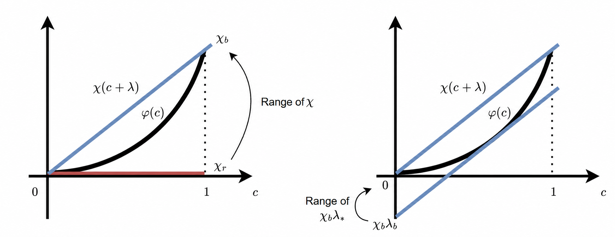
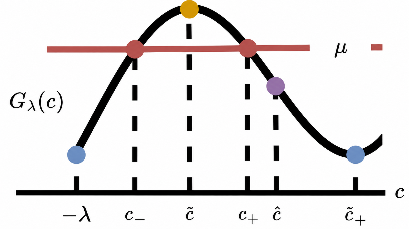
Figure 2. Left: Profile of the function GλG_{\lambda}. Right: Intersection points of φ\varphi and c↦χ(c+λ))c\mapsto\chi(c+\lambda)).

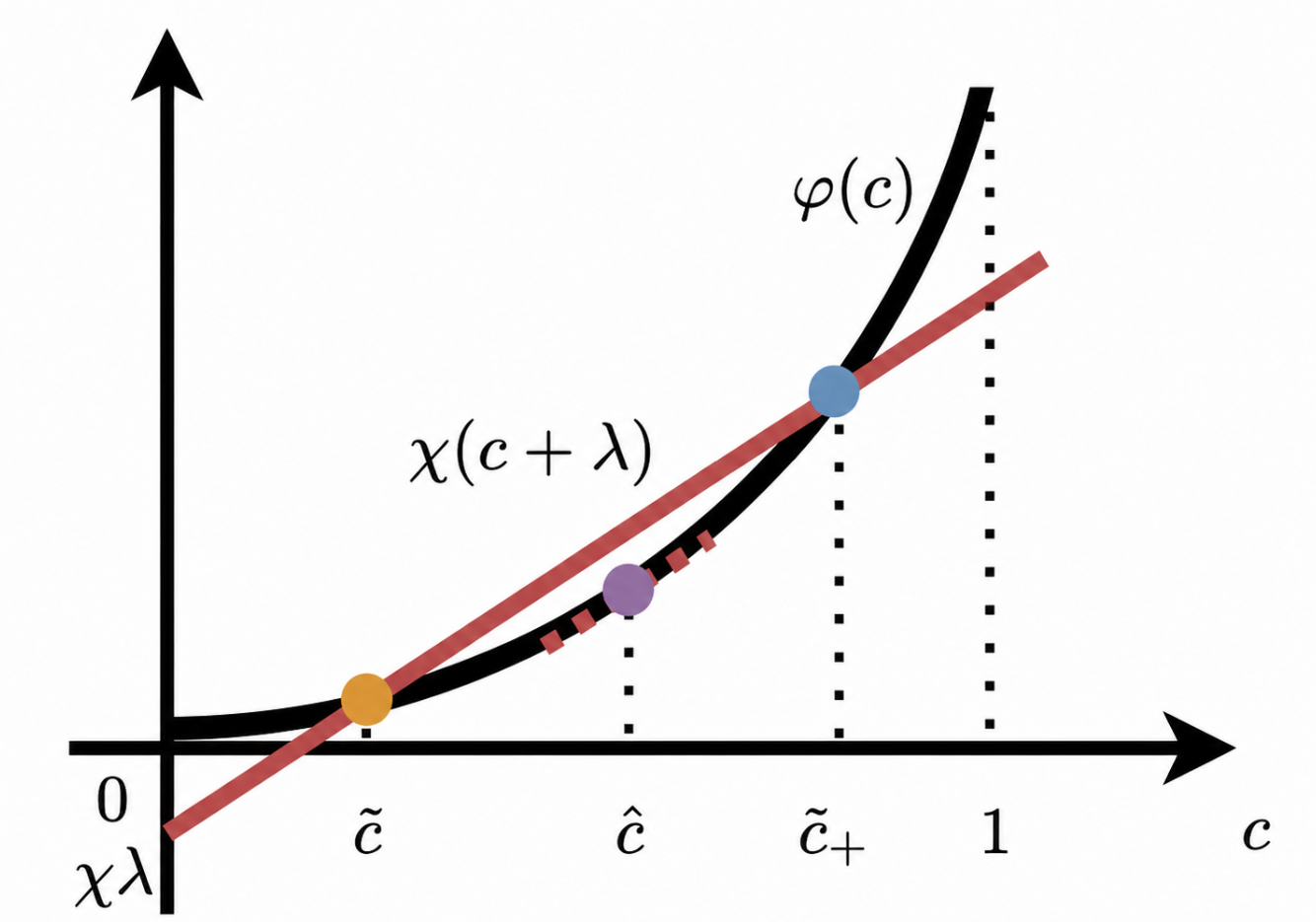
Before we prove this result, we study the profile of GλG_{\lambda}. We determine the parameter regime in which GλG_{\lambda} possesses two extremas c~\widetilde{c} and c~+\widetilde{c}_{+}; see Figure 2 (left). It holds 0=Gλ′​(c)=2​c−2​φ−1​(χ​(c+λ))0=G^{\prime}_{\lambda}(c)=2c-2\varphi^{-1}(\chi(c+\lambda)) if and only if

(34) cm−1m−1=φ​(c)=χ​(c+λ).\displaystyle\frac{c^{m-1}}{m-1}=\varphi(c)=\chi(c+\lambda).

This problem may have one or two solutions in [0,1][0,1], depending on the value of λ\lambda; see Figure 3 (right). The line c↦χ​(c+λ)c\mapsto\chi(c+\lambda) may intersect with the graph of φ\varphi only once. This happens if φ′​(c)=χ\varphi^{\prime}(c)=\chi, giving c=χ1/(m−2)c=\chi^{1/(m-2)}. Inserting this value into (34) leads to

χ(m−1)/(m−2)m−1=χ​(χ1/(m−2)+λ)and thusλ=−m−2m−1​χ1/(m−2)<0.\displaystyle\frac{\chi^{(m-1)/(m-2)}}{m-1}=\chi(\chi^{1/(m-2)}+\lambda)\quad\mbox{and thus}\quad\lambda=-\frac{m-2}{m-1}\chi^{1/(m-2)}<0.

On the other hand, if the line c↦χ​(c+λ)c\mapsto\chi(c+\lambda) is shifted upwards as in Figure 3 (right), there are two intersection points. Let one intersection point be equal to zero. The abscissa of the second intersection point may be larger than one, which is outside of the interval [0,1][0,1] and which does not provide a restriction on the value of λ\lambda. Let the abscissa equal to one (or smaller) and let χ≤1/(m−1)\chi\leq 1/(m-1). Then 0<c=φ−1​(χ​(c+λ))<10<c=\varphi^{-1}(\chi(c+\lambda))<1 implies that 1/(χ​(m−1))>1+λ1/(\chi(m-1))>1+\lambda and λ<0\lambda<0. Thus, we choose λ\lambda satisfying

−m−2m−1​χ1/(m−2)<λ<min⁡{0,1(m−1)​χ−1}=0.\displaystyle-\frac{m-2}{m-1}\chi^{1/(m-2)}<\lambda<\min\bigg\{0,\frac{1}{(m-1)\chi}-1\bigg\}=0.

For λ\lambda from this interval, there exist two solutions c~\widetilde{c} and c~+\widetilde{c}_{+} to (34) satisfying 0<c~<c~+<10<\widetilde{c}<\widetilde{c}_{+}<1. These two values are critical points of GλG_{\lambda}; see Figure 3 (left).

Refer to caption
Figure 3. Illustration of the solution to (34) with χr=0\chi_{r}=0 and χb=1/(m−1)\chi_{b}=1/(m-1).

We determine c^\widehat{c} such that

0=Gλ′′​(c)=2−2​χ​(φ−1)′​(χ​(c+λ))=2​(1−χφ′​(ρ)),\displaystyle 0=G^{\prime\prime}_{\lambda}(c)=2-2\chi(\varphi^{-1})^{\prime}(\chi(c+\lambda))=2\bigg(1-\frac{\chi}{\varphi^{\prime}(\rho)}\bigg),

recalling that ρ=φ−1​(χ​(c+λ))\rho=\varphi^{-1}(\chi(c+\lambda)). Since φ′​(0)=0\varphi^{\prime}(0)=0, φ′​(1)=1\varphi^{\prime}(1)=1, and φ′\varphi^{\prime} is increasing, there exists a unique ρ^\widehat{\rho} such that φ′​(ρ^)=χ\varphi^{\prime}(\widehat{\rho})=\chi. Then, defining c^\widehat{c} by ρ^=φ−1​(χ​(c^+λ))\widehat{\rho}=\varphi^{-1}(\chi(\widehat{c}+\lambda)), it holds that Gλ′′​(c^)=0G^{\prime\prime}_{\lambda}(\widehat{c})=0. Since φ′\varphi^{\prime} is positive, we have

Gλ′′​(c)<0if and only ifφ′​(ρ)<χif and only ifρ<ρ^,c<c^,\displaystyle G^{\prime\prime}_{\lambda}(c)<0\quad\mbox{if and only if}\quad\varphi^{\prime}(\rho)<\chi\quad\mbox{if and only if}\quad\rho<\widehat{\rho},\ c<\widehat{c},
Gλ′′​(c)>0if and only ifφ′​(ρ)>χif and only ifρ>ρ^,c>c^.\displaystyle G^{\prime\prime}_{\lambda}(c)>0\quad\mbox{if and only if}\quad\varphi^{\prime}(\rho)>\chi\quad\mbox{if and only if}\quad\rho>\widehat{\rho},\ c>\widehat{c}.

We know already that Gλ′′​(c~)<0G^{\prime\prime}_{\lambda}(\widetilde{c})<0. Furthermore, the inequality φ′​(ρ)>χ\varphi^{\prime}(\rho)>\chi is satisfied by c~+\widetilde{c}_{+} such that Gλ′′​(c~+)>0G^{\prime\prime}_{\lambda}(\widetilde{c}_{+})>0. This situation is illustrated in Figure 2 (left).

We show now that there exists λ∗<0\lambda^{*}<0 such that Gλ∗​(−λ∗)=Gλ∗​(c~+)G_{\lambda^{*}}(-\lambda^{*})=G_{\lambda^{*}}(\widetilde{c}_{+}).

Lemma 10.

Let m>2m>2 and χr:=0<χ<χb:=1/(m−1)\chi_{r}:=0<\chi<\chi_{b}:=1/(m-1). Then there exists λ∗\lambda^{*} satisfying

(35) −m−2m−1​χ1/(m−2)<λ∗<(1(π2+1)​(m−1)−1)​(χπ2+1)1/(m−2),\displaystyle-\frac{m-2}{m-1}\chi^{1/(m-2)}<\lambda^{*}<\bigg(\frac{1}{(\pi^{2}+1)(m-1)}-1\bigg)\bigg(\frac{\chi}{\pi^{2}+1}\bigg)^{1/(m-2)},

such that Gλ∗​(−λ∗)≤Gλ∗​(c~+)G_{\lambda^{*}}(-\lambda^{*})\leq G_{\lambda^{*}}(\widetilde{c}_{+}).

Remark 11.

We verify the well-posedness of (35), i.e., we show that

(36) m−2m−1>(1−1(π2+1)​(m−1))​(1π2+1)1/(m−2).\displaystyle\frac{m-2}{m-1}>\bigg(1-\frac{1}{(\pi^{2}+1)(m-1)}\bigg)\bigg(\frac{1}{\pi^{2}+1}\bigg)^{1/(m-2)}.

To this end, we introduce

F​(m)\displaystyle F(m) =log⁡m−2m−1−log⁡{(1−1(π2+1)​(m−1))​(1π2+1)1/(m−2)}\displaystyle=\log\frac{m-2}{m-1}-\log\bigg\{\bigg(1-\frac{1}{(\pi^{2}+1)(m-1)}\bigg)\bigg(\frac{1}{\pi^{2}+1}\bigg)^{1/(m-2)}\bigg\}
=log⁡(m−2)−log⁡(m−1)−log⁡(1−1(π2+1)​(m−1))+log⁡(π2+1)m−2.\displaystyle=\log(m-2)-\log(m-1)-\log\bigg(1-\frac{1}{(\pi^{2}+1)(m-1)}\bigg)+\frac{\log(\pi^{2}+1)}{m-2}.

Determining the values of the derivative

F′​(m)\displaystyle F^{\prime}(m) =((π2+2)−(π2+1)​m)​log⁡(π2+1)+π2​(m−2)(m−2)2​((π2+1)​m−(π2+2))\displaystyle=\frac{((\pi^{2}+2)-(\pi^{2}+1)m)\log(\pi^{2}+1)+\pi^{2}(m-2)}{(m-2)^{2}((\pi^{2}+1)m-(\pi^{2}+2))}
=−log⁡(π2+1)(m−2)2+π2(m−2)​((π2+1)​m−(π2+2))\displaystyle=-\frac{\log(\pi^{2}+1)}{(m-2)^{2}}+\frac{\pi^{2}}{(m-2)((\pi^{2}+1)m-(\pi^{2}+2))}

shows that F′​(m)<0F^{\prime}(m)<0 for m>2m>2. Then it follows from F​(m)→+∞F(m)\to+\infty as m→2+m\to 2^{+} and F​(m)→0F(m)\to 0 as m→∞m\to\infty that F​(m)>0F(m)>0 for all m>2m>2. This shows inequality (36).

Proof of Lemma 10.

Let χr<χ<χb\chi_{r}<\chi<\chi_{b}. We introduce the function

J​(χ,c):=Gλ​(c)−Gλ​(−λ)=c2−λ2−2​∫−λcφ−1​(χ​(z+λ))​𝑑z.\displaystyle J(\chi,c):=G_{\lambda}(c)-G_{\lambda}(-\lambda)=c^{2}-\lambda^{2}-2\int_{-\lambda}^{c}\varphi^{-1}(\chi(z+\lambda))dz.

Let λ=λb:=−(m−2)​χ1/(m−2)/(m−1)\lambda=\lambda_{b}:=-(m-2)\chi^{1/(m-2)}/(m-1). This corresponds to the case when the curves φ\varphi and c↦χ​(c+λ)c\mapsto\chi(c+\lambda) intersect at one point, implying that χ​(c+λ)\chi(c+\lambda) is below the curve φ\varphi, i.e. φ​(c)≥χ​(c+λ)\varphi(c)\geq\chi(c+\lambda) or c≥φ−1​(λ​(c+λ))c\geq\varphi^{-1}(\lambda(c+\lambda)) for all c∈(−λ,1)c\in(-\lambda,1). Consequently,

J​(χ,c)≥c2−λ2−2​∫−λcz​𝑑z=0for all ​c∈(−λ,1),\displaystyle J(\chi,c)\geq c^{2}-\lambda^{2}-2\int_{-\lambda}^{c}zdz=0\quad\mbox{for all }c\in(-\lambda,1),

which implies that Gλ​(−λ)≤Gλ​(c)G_{\lambda}(-\lambda)\leq G_{\lambda}(c).

Let λ=0\lambda=0. The intersection points of φ\varphi and c↦χ​cc\mapsto\chi c are exactly zero and c~+\widetilde{c}_{+}. We know that c~\widetilde{c} is an extremal point of GλG_{\lambda}. We find, for sufficiently small c>0c>0, that

G0​(0)−G0​(c)\displaystyle G_{0}(0)-G_{0}(c) =−c2+2​∫0cφ−1​(χ​z)​𝑑z=−c2+2​∫0c[(m−1)​χ​z]1/(m−1)​𝑑z\displaystyle=-c^{2}+2\int_{0}^{c}\varphi^{-1}(\chi z)dz=-c^{2}+2\int_{0}^{c}[(m-1)\chi z]^{1/(m-1)}dz
=c​(−c(m−2)/(m−1)+2​[(m−1)​χ]1/(m−1)​mm−1)>0,\displaystyle=c\bigg(-c^{(m-2)/(m-1)}+2[(m-1)\chi]^{1/(m-1)}\frac{m}{m-1}\bigg)>0,

so zero is a local maximum of GλG_{\lambda}, and since c~<c~+\widetilde{c}<\widetilde{c}_{+}, we infer that c~=0\widetilde{c}=0. The case λ=0\lambda=0 corresponds to the situation when the curve φ\varphi is below the line c↦χ​cc\mapsto\chi c, i.e. φ​(c)≤χ​c\varphi(c)\leq\chi c or c≤φ−1​(χ​c)c\leq\varphi^{-1}(\chi c) for all c∈(0,c~+)c\in(0,\widetilde{c}_{+}). Hence,

G0′​(c)=2​(c−φ−1​(χ​c))<0for ​c∈(0,c~+)\displaystyle G_{0}^{\prime}(c)=2(c-\varphi^{-1}(\chi c))<0\quad\mbox{for }c\in(0,\widetilde{c}_{+})

Consequently, G0​(c~+)<G0​(0)G_{0}(\widetilde{c}_{+})<G_{0}(0) and Gλ​(−λ)>Gλ​(c~+)G_{\lambda}(-\lambda)>G_{\lambda}(\widetilde{c}_{+}) for λ=0\lambda=0. By continuity, there exists λ∗\lambda^{*} in the desired range such that Gλ∗​(−λ∗)≤Gλ∗​(c~+)G_{\lambda^{*}}(-\lambda^{*})\leq G_{\lambda^{*}}(\widetilde{c}_{+}). ∎

We are now ready to prove Proposition 9.

Proof of Proposition 9.

The idea is to show that there exists μ∗\mu^{*} such that X​(λ∗,μ∗)=1X(\lambda^{*},\mu^{*})=1. First, we prove that there exists μ\mu such that X​(λ∗,μ)<1X(\lambda^{*},\mu)<1. Recall the boundary values c±=c±​(μ)c_{\pm}=c_{\pm}(\mu); see (33). A Taylor expansion of Gλ∗​(c)G_{\lambda^{*}}(c) around c~\widetilde{c} shows that

limμ→Gλ∗​(c~),c∈(c−​(μ),c+​(μ))Aμ​(c)=−12​Gλ∗′′​(c~),whereAμ​(c):=Gλ∗​(c)−μ(c+−c)​(c−c−).\displaystyle\lim_{\begin{subarray}{c}\mu\to G_{\lambda^{*}}(\widetilde{c}),\\ c\in(c_{-}(\mu),c_{+}(\mu))\end{subarray}}A_{\mu}(c)=-\frac{1}{2}G^{\prime\prime}_{\lambda^{*}}(\widetilde{c}),\quad\mbox{where}\quad A_{\mu}(c):=\frac{G_{\lambda^{*}}(c)-\mu}{(c_{+}-c)(c-c_{-})}.

We set

c​(z):=z2​(c+​(μ)−c−​(μ))+12​(c+​(μ)+c−​(μ))for ​z∈[−1,1].\displaystyle c(z):=\frac{z}{2}\big(c_{+}(\mu)-c_{-}(\mu)\big)+\frac{1}{2}\big(c_{+}(\mu)+c_{-}(\mu)\big)\quad\mbox{for }z\in[-1,1].

Observing that c​(±1)=c±​(μ)c(\pm 1)=c_{\pm}(\mu), a substitution leads to

X​(λ∗,μ)\displaystyle X(\lambda^{*},\mu) =∫c−​(μ)c+​(μ)d​cGλ∗​(c)−μ=∫c−​(μ)c+​(μ)d​c(c+​(μ)−c)​(c−c−​(μ))​Aμ​(c)\displaystyle=\int_{c_{-}(\mu)}^{c_{+}(\mu)}\frac{dc}{\sqrt{G_{\lambda^{*}}(c)-\mu}}=\int_{c_{-}(\mu)}^{c_{+}(\mu)}\frac{dc}{\sqrt{(c_{+}(\mu)-c)(c-c_{-}(\mu))A_{\mu}(c)}}
=∫−11d​z(1−z)​(1+z)​Aμ​(c​(z)).\displaystyle=\int_{-1}^{1}\frac{dz}{\sqrt{(1-z)(1+z)A_{\mu}(c(z))}}.

By dominated convergence,

limμ→Gλ∗​(c~)X​(λ∗,μ)=limμ→Gλ∗​(c~)∫−112​d​z−(1−z)​(1+z)​Gλ∗′′​(v~)=2​π−Gλ∗′′​(v~).\displaystyle\lim_{\mu\to G_{\lambda^{*}}(\widetilde{c})}X(\lambda^{*},\mu)=\lim_{\mu\to G_{\lambda^{*}}(\widetilde{c})}\int_{-1}^{1}\frac{\sqrt{2}dz}{\sqrt{-(1-z)(1+z)G^{\prime\prime}_{\lambda^{*}}(\widetilde{v})}}=\frac{\sqrt{2}\pi}{\sqrt{-G^{\prime\prime}_{\lambda^{*}}(\widetilde{v})}}.

We claim that Gλ∗′′​(c~)<−2​π2G^{\prime\prime}_{\lambda^{*}}(\widetilde{c})<-2\pi^{2}. Then, choosing μ\mu smaller than but close to Gλ∗′′​(c~)G^{\prime\prime}_{\lambda^{*}}(\widetilde{c}), we obtain X​(λ∗,μ)<1X(\lambda^{*},\mu)<1. To prove the claim, we recall that Gλ∗′′​(c~)=2​(1−χ/φ′​(c~))G^{\prime\prime}_{\lambda^{*}}(\widetilde{c})=2(1-\chi/\varphi^{\prime}(\widetilde{c})). Therefore, the inequality Gλ∗′′​(c~)<−2​π2G^{\prime\prime}_{\lambda^{*}}(\widetilde{c})<-2\pi^{2} is equivalent to

(37) (π2+1)​c~m−2=(π2+1)​φ′​(c~)<χ=φ​(c~)c~+λ∗=c~m−1(m−1)​(c~+λ∗).\displaystyle(\pi^{2}+1)\widetilde{c}^{m-2}=(\pi^{2}+1)\varphi^{\prime}(\widetilde{c})<\chi=\frac{\varphi(\widetilde{c})}{\widetilde{c}+\lambda^{*}}=\frac{\widetilde{c}^{m-1}}{(m-1)(\widetilde{c}+\lambda^{*})}.

We solve this inequality for λ∗\lambda^{*}:

λ∗<c~​(1(π2+1)​(m−1)−1).\displaystyle\lambda^{*}<\widetilde{c}\bigg(\frac{1}{(\pi^{2}+1)(m-1)}-1\bigg).

This inequality holds true in view of our assumption (35) and the property c~<(χ/(π2+1))1/(m−2)\widetilde{c}<(\chi/(\pi^{2}+1))^{1/(m-2)} from (37).

Next, we prove that X​(λ∗,μ)=+∞X(\lambda^{*},\mu)=+\infty if μ=Gλ∗​(c~+)\mu=G_{\lambda^{*}}(\widetilde{c}_{+}). We observe that in this case c+=c~+c_{+}=\widetilde{c}_{+} and Gλ∗′​(c+)=0G^{\prime}_{\lambda^{*}}(c_{+})=0, Gλ∗′′​(c+)>0G^{\prime\prime}_{\lambda^{*}}(c_{+})>0 (see Figure 2 left). Then, by Taylor expansion around c+c_{+},

limc→c+c+−cGλ∗​(c)−Gλ∗​(c+)\displaystyle\lim_{c\to c_{+}}\frac{c_{+}-c}{\sqrt{G_{\lambda^{*}}(c)-G_{\lambda^{*}}(c_{+})}} =limc→c+c−c+Gλ∗​(c+)​(c−c+)2/2+o​((c−c+)2)\displaystyle=\lim_{c\to c_{+}}\frac{c-c_{+}}{\sqrt{G_{\lambda^{*}}(c_{+})(c-c_{+})^{2}/2+o((c-c_{+})^{2})}}
=2Gλ∗′′​(c+)>0.\displaystyle=\sqrt{\frac{2}{G_{\lambda^{*}}^{\prime\prime}(c_{+})}}>0.

Thus, the integrand of

X​(λ∗,μ)=∫c−c+d​zGλ∗​(z)−Gλ∗​(c+)\displaystyle X(\lambda^{*},\mu)=\int_{c_{-}}^{c_{+}}\frac{dz}{\sqrt{G_{\lambda^{*}}(z)-G_{\lambda^{*}}(c_{+})}}

behaves like 1/(c+−c)1/(c_{+}-c) for c→c+c\to c_{+}, which means that X​(λ∗,μ)X(\lambda^{*},\mu) diverges. This shows that X​(λ∗,μ)=+∞X(\lambda^{*},\mu)=+\infty, proving the claim. ∎

5. Long-time behavior of solutions

We have shown in the previous section that for 1<m≤21<m\leq 2 and χ≤1\chi\leq 1, the unique steady state to (1)–(3) is the constant pair (M,M)(M,M) (if |Ω|=1|\Omega|=1). In this section, we show that the solution constructed in Theorem 1 converges to this steady state as t→∞t\to\infty.

Recall definition (5) of the relative entropy H1H_{1} and let |Ω|=1|\Omega|=1. We deduce from (23) and mass conservation that

H1​(ρ,c|M,M)|st\displaystyle H_{1}(\rho,c|M,M)\Big|_{s}^{t} =∫Ω(ρ​(log⁡ρ−1)+(1−ρ)​(log⁡(1−ρ)−1))​𝑑x|st−τ​∫st∫Ω∂tc​Δ​c​d​x​d​s\displaystyle=\int_{\Omega}\big(\rho(\log\rho-1)+(1-\rho)(\log(1-\rho)-1)\big)dx\Big|_{s}^{t}-\tau\int_{s}^{t}\int_{\Omega}\partial_{t}c\Delta cdxds
≤−∫st∫Ωρm−2​|∇ρ|2​𝑑x​𝑑s+(χ+1)​∫st∫Ω∇ρ⋅∇c​d​x​d​s\displaystyle\leq-\int_{s}^{t}\int_{\Omega}\rho^{m-2}|\nabla\rho|^{2}dxds+(\chi+1)\int_{s}^{t}\int_{\Omega}\nabla\rho\cdot\nabla cdxds
−∫st∫Ω(η​(Δ​c)2+|∇c|2)​𝑑x​𝑑s.\displaystyle\phantom{xx}-\int_{s}^{t}\int_{\Omega}(\eta(\Delta c)^{2}+|\nabla c|^{2})dxds.

We use the Poincaré inequality

K1​∫Ω|∇c|2​𝑑x≤∫Ω|Δ​c|2​𝑑x,\displaystyle K_{1}\int_{\Omega}|\nabla c|^{2}dx\leq\int_{\Omega}|\Delta c|^{2}dx,

where K1>0K_{1}>0 is the principal Neumann eigenvalue (see the proof of [8, Theorem 2.1]), Young’s inequality with ε>0\varepsilon>0, the property ρm−2≥1\rho^{m-2}\geq 1 (which follows from m≤2m\leq 2), and the bound χ≤1\chi\leq 1 to estimate as follows:

H1\displaystyle H_{1} (ρ,c|M,M)|st≤−∫st∫Ω(ρm−2​|∇ρ|2+(η​K1+1)​|∇c|2)​𝑑x​𝑑σ\displaystyle(\rho,c|M,M)\Big|_{s}^{t}\leq-\int_{s}^{t}\int_{\Omega}\big(\rho^{m-2}|\nabla\rho|^{2}+(\eta K_{1}+1)|\nabla c|^{2}\big)dxd\sigma
+(χ+1)​∫0t∫Ω∇ρ⋅∇c​d​x​d​σ\displaystyle\phantom{xx}+(\chi+1)\int_{0}^{t}\int_{\Omega}\nabla\rho\cdot\nabla cdxd\sigma
≤−∫st∫Ω{(1−11+ε)​|∇ρ|2+(η​K1+1−1+ε4​(χ+1)2)​|∇c|2}​𝑑x​𝑑σ.\displaystyle\leq-\int_{s}^{t}\int_{\Omega}\bigg\{\bigg(1-\frac{1}{1+\varepsilon}\bigg)|\nabla\rho|^{2}+\bigg(\eta K_{1}+1-\frac{1+\varepsilon}{4}(\chi+1)^{2}\bigg)|\nabla c|^{2}\bigg\}dxd\sigma.

Since χ≤1\chi\leq 1, the choice ε=η​K1\varepsilon=\eta K_{1} leads to

η​K1+1−1+ε4​(χ+1)2≥η​K1+1−(1+ε)=0\displaystyle\eta K_{1}+1-\frac{1+\varepsilon}{4}(\chi+1)^{2}\geq\eta K_{1}+1-(1+\varepsilon)=0

and hence to

(38) H1​(ρ,c|M,M)|st≤−(1−11+η​K1)​∫st∫Ω|∇ρ|2​𝑑x​𝑑σ.\displaystyle H_{1}(\rho,c|M,M)\Big|_{s}^{t}\leq-\bigg(1-\frac{1}{1+\eta K_{1}}\bigg)\int_{s}^{t}\int_{\Omega}|\nabla\rho|^{2}dxd\sigma.

We use the following variant of the logarithmic Sobolev inequality [1, Theorem 1]:

∫Ωρ​log⁡ρM​d​x\displaystyle\int_{\Omega}\rho\log\frac{\rho}{M}dx ≤C​(Ω)​M​∫Ω|∇ρ|2​𝑑x,\displaystyle\leq C(\Omega)M\int_{\Omega}|\nabla\rho|^{2}dx,
∫Ω(1−ρ)​log⁡1−ρ1−M​d​x\displaystyle\int_{\Omega}(1-\rho)\log\frac{1-\rho}{1-M}dx ≤C​(Ω)​(1−M)​∫Ω|∇ρ|2​𝑑x,\displaystyle\leq C(\Omega)(1-M)\int_{\Omega}|\nabla\rho|^{2}dx,

where C​(Ω)>1C(\Omega)>1 only depends on dd and the diameter of Ω\Omega, implying that

∫Ω(ρ​log⁡ρM+(1−ρ)​log⁡1−ρ1−M)​𝑑x≤C​(Ω)​∫Ω|∇ρ|2​𝑑x.\displaystyle\int_{\Omega}\bigg(\rho\log\frac{\rho}{M}+(1-\rho)\log\frac{1-\rho}{1-M}\bigg)dx\leq C(\Omega)\int_{\Omega}|\nabla\rho|^{2}dx.

Then (38) becomes

H1​(ρ,c|M,M)|st≤−μ0​∫stH1​(ρ,c|M,M)​𝑑x​𝑑σ,where​μ0=1C​(Ω)​η​K11+η​K1,\displaystyle H_{1}(\rho,c|M,M)\Big|_{s}^{t}\leq-\mu_{0}\int_{s}^{t}H_{1}(\rho,c|M,M)dxd\sigma,\quad\mbox{where}\ \mu_{0}=\frac{1}{C(\Omega)}\frac{\eta K_{1}}{1+\eta K_{1}},

and after division by s−ts-t and passing to the limit s→ts\to t,

dd​t​H1​(ρ,c|M,M)≤−μ0​H1​(ρ,c|M,M).\displaystyle\frac{d}{dt}H_{1}(\rho,c|M,M)\leq-\mu_{0}H_{1}(\rho,c|M,M).

We conclude from Gronwall’s inequality that

H1​(ρ​(t),c​(t)|M,M)≤H1​(ρ0,c0|M,M)​e−μ0​t,t>0.\displaystyle H_{1}(\rho(t),c(t)|M,M)\leq H_{1}(\rho^{0},c^{0}|M,M)e^{-\mu_{0}t},\quad t>0.

A Taylor expansion around MM leads for some ξ\xi between ρ\rho and MM to

ρ​log⁡ρM+(1−ρ)​log⁡1−ρ1−M=12​(ρ−M)2ξ​(1−ξ)≥2​(ρ−M)2.\displaystyle\rho\log\frac{\rho}{M}+(1-\rho)\log\frac{1-\rho}{1-M}=\frac{1}{2}\frac{(\rho-M)^{2}}{\xi(1-\xi)}\geq 2(\rho-M)^{2}.

This shows that

(39) 2​‖ρ​(t)−M‖L2​(Ω)2≤H1​(ρ0,c0|M,M)​e−μ0​t.\displaystyle 2\|\rho(t)-M\|_{L^{2}(\Omega)}^{2}\leq H_{1}(\rho^{0},c^{0}|M,M)e^{-\mu_{0}t}.

The exponential decay of c​(t)c(t) follows from (39). Indeed, using the test function c−Mc-M, we find from (2) that

τ2​dd​t​∫Ω(c−M)2​𝑑x\displaystyle\frac{\tau}{2}\frac{d}{dt}\int_{\Omega}(c-M)^{2}dx +∫Ω(η​|∇(c−M)|2+(c−M)2)​𝑑x=∫Ω(ρ−M)​(c−M)​𝑑x\displaystyle+\int_{\Omega}\big(\eta|\nabla(c-M)|^{2}+(c-M)^{2}\big)dx=\int_{\Omega}(\rho-M)(c-M)dx
≤−12​∫Ω(c−M)2​𝑑x+12​∫Ω(ρ−M)2​𝑑x\displaystyle\leq-\frac{1}{2}\int_{\Omega}(c-M)^{2}dx+\frac{1}{2}\int_{\Omega}(\rho-M)^{2}dx

and hence,

τ​dd​t​∫Ω(c−M)2​𝑑x+∫Ω(c−M)2​𝑑x≤∫Ω(ρ−M)2​𝑑x≤12​H1​(ρ0,c0|M,M)​e−μ0​t.\displaystyle\tau\frac{d}{dt}\int_{\Omega}(c-M)^{2}dx+\int_{\Omega}(c-M)^{2}dx\leq\int_{\Omega}(\rho-M)^{2}dx\leq\frac{1}{2}H_{1}(\rho^{0},c^{0}|M,M)e^{-\mu_{0}t}.

We apply Gronwall’s inequality:

‖c​(t)−M‖L2​(Ω)2≤C​e−min⁡{1/τ,μ0}​t,t>0,\displaystyle\|c(t)-M\|_{L^{2}(\Omega)}^{2}\leq Ce^{-\min\{1/\tau,\mu_{0}\}t},\quad t>0,

where C>0C>0 depends on τ\tau, (ρ0,c0)(\rho^{0},c^{0}), and Ω\Omega. With the test function −Δ​(c−M)-\Delta(c-M), we infer that

τ2​dd​t\displaystyle\frac{\tau}{2}\frac{d}{dt} ∫Ω|∇(c−M)|2​𝑑x+∫Ω(η​|Δ​(c−M)|2+|∇(c−M)|2)​𝑑x\displaystyle\int_{\Omega}|\nabla(c-M)|^{2}dx+\int_{\Omega}\big(\eta|\Delta(c-M)|^{2}+|\nabla(c-M)|^{2}\big)dx
=−∫Ω(ρ−M)Δ(c−M)dx≤η∫Ω|Δ(c−M)|2+η4∫Ω(ρ−M)|2dx.\displaystyle=-\int_{\Omega}(\rho-M)\Delta(c-M)dx\leq\eta\int_{\Omega}|\Delta(c-M)|^{2}+\frac{\eta}{4}\int_{\Omega}(\rho-M)|^{2}dx.

Applying Gronwall’s inequality again leads to

‖∇(c​(t)−M)‖L2​(Ω)2≤C​e−min⁡{1/τ,μ0}​t,t>0,\displaystyle\|\nabla(c(t)-M)\|_{L^{2}(\Omega)}^{2}\leq Ce^{-\min\{1/\tau,\mu_{0}\}t},\quad t>0,

finishing the proof of Theorem 3.

6. Asymptotic limits

In this section, we prove the asymptotic limits τ→0\tau\to 0 (Theorem 4) and η→0\eta\to 0 (Theorem 5).

6.1. Parabolic–elliptic limit

We wish to perform the limit τ→0\tau\to 0 in equations (1)–(2), leading to the parabolic–elliptic Keller–Segel model. Let (ρτ,cτ)(\rho_{\tau},c_{\tau}) be a solution to

(40) ∂tρτ\displaystyle\partial_{t}\rho_{\tau} =div⁡((1−ρτ)​ρτm−1​∇ρτ−χ​ρτ​(1−ρτ)​∇cτ),\displaystyle=\operatorname{div}\big((1-\rho_{\tau})\rho_{\tau}^{m-1}\nabla\rho_{\tau}-\chi\rho_{\tau}(1-\rho_{\tau})\nabla c_{\tau}\big),
τ​∂tcτ\displaystyle\tau\partial_{t}c_{\tau} =η​Δ​cτ−cτ+ρτin ​Ω,t>0,\displaystyle=\eta\Delta c_{\tau}-c_{\tau}+\rho_{\tau}\quad\mbox{in }\Omega,\ t>0,

satisfying the initial and no-flux boundary conditions (3). The proof is based on uniform estimates derived from the entropy functional (8).

Lemma 12.

Let (ρτ,cτ)(\rho_{\tau},c_{\tau}) be a weak solution to (3), (40). Then there exists a constant C>0C>0, independent of τ\tau, such that

Fτ​(ρτ,cτ)|0t+12​∫0t∫Ωρτm−2​|∇ρτ|2​𝑑x​𝑑s≤C​τ.\displaystyle F_{\tau}(\rho_{\tau},c_{\tau})\Big|_{0}^{t}+\frac{1}{2}\int_{0}^{t}\int_{\Omega}\rho_{\tau}^{m-2}|\nabla\rho_{\tau}|^{2}dxds\leq C\tau.
Proof.

We sum (23), rewritten as

∫Ω(ρτ(logρτ−1)\displaystyle\int_{\Omega}\big(\rho_{\tau}(\log\rho_{\tau}-1) +(1−ρτ)(log(1−ρτ)−1))dx|0t+∫0t∫Ωρτm−2|∇ρτ|2dxds\displaystyle+(1-\rho_{\tau})(\log(1-\rho_{\tau})-1)\big)dx\Big|_{0}^{t}+\int_{0}^{t}\int_{\Omega}\rho_{\tau}^{m-2}|\nabla\rho_{\tau}|^{2}dxds
≤χ​∫0t∫Ω∇ρτ⋅∇cτ​d​x​d​s,\displaystyle\leq\chi\int_{0}^{t}\int_{\Omega}\nabla\rho_{\tau}\cdot\nabla c_{\tau}dxds,

and

τ​χη​∫Ωρτ​cτ​𝑑x|0t\displaystyle\frac{\tau\chi}{\eta}\int_{\Omega}\rho_{\tau}c_{\tau}dx\Big|_{0}^{t} =τ​χη​∫0t⟨∂tρτ,cτ⟩​𝑑s+τ​χη​∫0t∫Ωρτ​∂tcτ​d​x​d​s\displaystyle=\frac{\tau\chi}{\eta}\int_{0}^{t}\langle\partial_{t}\rho_{\tau},c_{\tau}\rangle ds+\frac{\tau\chi}{\eta}\int_{0}^{t}\int_{\Omega}\rho_{\tau}\partial_{t}c_{\tau}dxds
=−τ​χη​∫0t∫Ω((1−ρτ)​ρτm−1​∇ρτ⋅∇cτ−χ​ρτ​(1−ρτ)​|∇cτ|2)​𝑑x​𝑑s\displaystyle=-\frac{\tau\chi}{\eta}\int_{0}^{t}\int_{\Omega}\big((1-\rho_{\tau})\rho_{\tau}^{m-1}\nabla\rho_{\tau}\cdot\nabla c_{\tau}-\chi\rho_{\tau}(1-\rho_{\tau})|\nabla c_{\tau}|^{2}\big)dxds
−χ​∫0t∫Ω∇ρτ⋅∇cτ​d​x​d​s+χη​∫0t∫Ω(ρτ−cτ)​ρτ​𝑑x​𝑑s.\displaystyle\phantom{xx}-\chi\int_{0}^{t}\int_{\Omega}\nabla\rho_{\tau}\cdot\nabla c_{\tau}dxds+\frac{\chi}{\eta}\int_{0}^{t}\int_{\Omega}(\rho_{\tau}-c_{\tau})\rho_{\tau}dxds.

Then the term involving ∇ρτ⋅∇cτ\nabla\rho_{\tau}\cdot\nabla c_{\tau} cancels and, observing that (ρτ−cτ)​cτ≤1(\rho_{\tau}-c_{\tau})c_{\tau}\leq 1 and applying Young’s inequality, we obtain

Fτ​(ρτ,cτ)|0t\displaystyle F_{\tau}(\rho_{\tau},c_{\tau})\Big|_{0}^{t} +∫0t∫Ωρτm−2​|∇ρτ|2​𝑑x​𝑑s\displaystyle+\int_{0}^{t}\int_{\Omega}\rho_{\tau}^{m-2}|\nabla\rho_{\tau}|^{2}dxds
≤12​∫0t∫Ωρτm−2​|∇ρτ|2​𝑑x​𝑑s+12​(τ​χη)2​∫0t∫Ω(1−ρτ)2​ρτm​|∇cτ|2​𝑑x​𝑑s\displaystyle\leq\frac{1}{2}\int_{0}^{t}\int_{\Omega}\rho_{\tau}^{m-2}|\nabla\rho_{\tau}|^{2}dxds+\frac{1}{2}\bigg(\frac{\tau\chi}{\eta}\bigg)^{2}\int_{0}^{t}\int_{\Omega}(1-\rho_{\tau})^{2}\rho_{\tau}^{m}|\nabla c_{\tau}|^{2}dxds
+τ​χ2η​∫0t∫Ωρτ​(1−ρτ)​|∇cτ|2​𝑑x​𝑑s+χ​meas​(ΩT).\displaystyle\phantom{xx}+\frac{\tau\chi^{2}}{\eta}\int_{0}^{t}\int_{\Omega}\rho_{\tau}(1-\rho_{\tau})|\nabla c_{\tau}|^{2}dxds+\chi\mbox{meas}(\Omega_{T}).

Using the test function cτc_{\tau} in equation (2) gives

τ​∫Ωcτ​(t)2​𝑑x−τ​∫Ω(c0)2​𝑑x+∫0t∫Ω(η​|∇cτ|2+cτ2)​𝑑x​𝑑s=∫0t∫Ωρτ​cτ​𝑑x​𝑑s≤C,\displaystyle\tau\int_{\Omega}c_{\tau}(t)^{2}dx-\tau\int_{\Omega}(c^{0})^{2}dx+\int_{0}^{t}\int_{\Omega}\big(\eta|\nabla c_{\tau}|^{2}+c_{\tau}^{2}\big)dxds=\int_{0}^{t}\int_{\Omega}\rho_{\tau}c_{\tau}dxds\leq C,

and we conclude a uniform bound for (cτ)(c_{\tau}) in L2​(0,T;H1​(Ω))L^{2}(0,T;H^{1}(\Omega)), finishing the proof. ∎

Lemma 13.

Let c0∈H1​(Ω)c^{0}\in H^{1}(\Omega). Then there exists C>0C>0 independent of τ\tau such that

τ​‖∂tcτ‖L2​(ΩT)+‖cτ‖L∞​(0,T;H1​(Ω))≤C.\displaystyle\sqrt{\tau}\|\partial_{t}c_{\tau}\|_{L^{2}(\Omega_{T})}+\|c_{\tau}\|_{L^{\infty}(0,T;H^{1}(\Omega))}\leq C.
Proof.

We multiply the second equation in (40) by ∂tcτ\partial_{t}c_{\tau}, integrate over Ω\Omega and (0,t)(0,t), and integrate by parts:

τ\displaystyle\tau ∫0t∫Ω(∂tcτ)2​𝑑x​𝑑s=−∫0t∫Ω(η​Δ​cτ−cτ+ρτ)​∂tcτ​d​x​d​s\displaystyle\int_{0}^{t}\int_{\Omega}(\partial_{t}c_{\tau})^{2}dxds=-\int_{0}^{t}\int_{\Omega}(\eta\Delta c_{\tau}-c_{\tau}+\rho_{\tau})\partial_{t}c_{\tau}dxds
=−12​∫Ω(η​|∇cτ|2+cτ)​𝑑x|0t+∫0tdd​t​∫Ωρτ​cτ​𝑑x​𝑑s−∫0t⟨∂tρτ,cτ⟩​𝑑s\displaystyle=-\frac{1}{2}\int_{\Omega}\big(\eta|\nabla c_{\tau}|^{2}+c_{\tau}\big)dx\Big|_{0}^{t}+\int_{0}^{t}\frac{d}{dt}\int_{\Omega}\rho_{\tau}c_{\tau}dxds-\int_{0}^{t}\langle\partial_{t}\rho_{\tau},c_{\tau}\rangle ds
≤−12​∫Ω(η​|∇cτ​(t)|2+cτ​(t)2)​𝑑x+∫Ωρτ​(t)​cτ​(t)​𝑑x\displaystyle\leq-\frac{1}{2}\int_{\Omega}\big(\eta|\nabla c_{\tau}(t)|^{2}+c_{\tau}(t)^{2}\big)dx+\int_{\Omega}\rho_{\tau}(t)c_{\tau}(t)dx
+‖∂tρτ‖L2​(0,T;H1​(Ω)′)​‖cτ‖L2​(0,T;H1​(Ω))+C​(ρ0,c0)\displaystyle\phantom{xx}+\|\partial_{t}\rho_{\tau}\|_{L^{2}(0,T;H^{1}(\Omega)^{\prime})}\|c_{\tau}\|_{L^{2}(0,T;H^{1}(\Omega))}+C(\rho^{0},c^{0})
≤−12​∫Ω(η​|∇cτ​(t)|2+cτ​(t)2)​𝑑x+C,\displaystyle\leq-\frac{1}{2}\int_{\Omega}\big(\eta|\nabla c_{\tau}(t)|^{2}+c_{\tau}(t)^{2}\big)dx+C,

where the last step follows from Lemma 12 and ρτ≤1\rho_{\tau}\leq 1 and cτ≤1c_{\tau}\leq 1. This concludes the proof. ∎

We deduce from Lemma 12 that (ρτm/2)(\rho_{\tau}^{m/2}) is bounded in L2​(0,T;H1​(Ω))L^{2}(0,T;H^{1}(\Omega)) and

‖∂tρτ‖L2​(0,T;H1​(Ω)′)≤‖2m​(1−ρτ)​ρτm/2​∇ρτm/2−χ​ρτ​(1−ρτ)​∇cτ‖L2​(ΩT)≤C\displaystyle\|\partial_{t}\rho_{\tau}\|_{L^{2}(0,T;H^{1}(\Omega)^{\prime})}\leq\bigg\|\frac{2}{m}(1-\rho_{\tau})\rho_{\tau}^{m/2}\nabla\rho_{\tau}^{m/2}-\chi\rho_{\tau}(1-\rho_{\tau})\nabla c_{\tau}\bigg\|_{L^{2}(\Omega_{T})}\leq C

for some C>0C>0 independent of τ\tau. This allows us to apply the Aubin–Lions lemma in the version of [20] to conclude the existence of a subsequence that is not relabeled such that

ρτ→ρstrongly in ​L2​(ΩT)​as ​τ→0.\displaystyle\rho_{\tau}\to\rho\quad\mbox{strongly in }L^{2}(\Omega_{T})\ \mbox{as }\tau\to 0.

Because of the uniform L∞​(ΩT)L^{\infty}(\Omega_{T}) bound for ρτ\rho_{\tau}, the family (ρτ)(\rho_{\tau}) converges strongly in any Lp​(ΩT)L^{p}(\Omega_{T}) with p<∞p<\infty. Lemma 12 shows that (cτ)(c_{\tau}) is bounded in L2​(0,T;H1​(Ω))L^{2}(0,T;H^{1}(\Omega)), hence, for a subsequence, cτ⇀cc_{\tau}\rightharpoonup c and ∇cτ⇀∇c\nabla c_{\tau}\rightharpoonup\nabla c weakly in L2​(ΩT)L^{2}(\Omega_{T}). By Lemma 13, τ​∂tcτ→0\tau\partial_{t}c_{\tau}\to 0 strongly in L2​(ΩT)L^{2}(\Omega_{T}). Furthermore, the following weak convergences hold (up to subsequences):

∇ρτm/2⇀∇ρm/2weakly in ​L2​(ΩT),∂tρτ⇀∂tρweakly in ​L2​(0,T;H1​(Ω)′).\displaystyle\nabla\rho_{\tau}^{m/2}\rightharpoonup\nabla\rho^{m/2}\quad\mbox{weakly in }L^{2}(\Omega_{T}),\quad\partial_{t}\rho_{\tau}\rightharpoonup\partial_{t}\rho\quad\mbox{weakly in }L^{2}(0,T;H^{1}(\Omega)^{\prime}).

This implies that

(1−ρτ)​ρτm−1​∇ρτ=2m​(1−ρτ)​ρτm/2​∇ρτm/2⇀2m​(1−ρ)​ρm/2​∇ρm/2=(1−ρ)​ρm−1​∇ρ\displaystyle(1-\rho_{\tau})\rho_{\tau}^{m-1}\nabla\rho_{\tau}=\frac{2}{m}(1-\rho_{\tau})\rho_{\tau}^{m/2}\nabla\rho_{\tau}^{m/2}\rightharpoonup\frac{2}{m}(1-\rho)\rho^{m/2}\nabla\rho^{m/2}=(1-\rho)\rho^{m-1}\nabla\rho

weakly in L1​(ΩT)L^{1}(\Omega_{T}), and since (1−ρτ)​ρτm/2​∇ρτm/2(1-\rho_{\tau})\rho_{\tau}^{m/2}\nabla\rho_{\tau}^{m/2} is uniformly bounded in L2​(ΩT)L^{2}(\Omega_{T}), this convergence also holds in L2​(ΩT)L^{2}(\Omega_{T}). Similarly,

ρτ​(1−ρτ)​∇cτ⇀ρ​(1−ρ)​∇cweakly in ​L2​(ΩT).\displaystyle\rho_{\tau}(1-\rho_{\tau})\nabla c_{\tau}\rightharpoonup\rho(1-\rho)\nabla c\quad\mbox{weakly in }L^{2}(\Omega_{T}).

Thus, we can pass to the limit τ→0\tau\to 0 in the weak formulation of (40) to infer that (ρ,c)(\rho,c) solves equations (6), together with the initial and boundary conditions (3).

6.2. Vanishing diffusion limit

The aim is the limit η→0\eta\to 0 in equations (1)–(2). Let (ρη,cη)(\rho_{\eta},c_{\eta}) be a weak solution to (1)–(2).

Lemma 14.

Let 1<m≤21<m\leq 2. Then there exists C>0C>0, independent of η\eta, such that

(41) ‖ρη‖L2​(0,T;H1​(Ω))+‖cη‖L2​(0,T;H1​(Ω))+η​‖Δ​cη‖L2​(ΩT)≤C​(T),\displaystyle\|\rho_{\eta}\|_{L^{2}(0,T;H^{1}(\Omega))}+\|c_{\eta}\|_{L^{2}(0,T;H^{1}(\Omega))}+\sqrt{\eta}\|\Delta c_{\eta}\|_{L^{2}(\Omega_{T})}\leq C(T),
Proof.

We compute, using Young’s inequality,

τ2​∫Ω|∇cη|2​𝑑x|0t\displaystyle\frac{\tau}{2}\int_{\Omega}|\nabla c_{\eta}|^{2}dx\Big|_{0}^{t} =−∫0t∫Ω(η​Δ​cη−cε+ρη)​Δ​cη​𝑑x​𝑑s\displaystyle=-\int_{0}^{t}\int_{\Omega}(\eta\Delta c_{\eta}-c_{\varepsilon}+\rho_{\eta})\Delta c_{\eta}dxds
=−∫0t∫Ω(η​(Δ​cη)2+|∇cη|2)​𝑑x​𝑑s+∫0t∫Ω∇ρε⋅∇cε​d​x​d​s.\displaystyle=-\int_{0}^{t}\int_{\Omega}\big(\eta(\Delta c_{\eta})^{2}+|\nabla c_{\eta}|^{2}\big)dxds+\int_{0}^{t}\int_{\Omega}\nabla\rho_{\varepsilon}\cdot\nabla c_{\varepsilon}dxds.

The condition 1<m≤21<m\leq 2 implies that ρεm−2≥1\rho_{\varepsilon}^{m-2}\geq 1. Therefore, taking into account (23) and the previous computation, recalling definition (9) of FηF_{\eta} and summing the expressions,

(42) Fη​(ρη,cη)|0t\displaystyle F_{\eta}(\rho_{\eta},c_{\eta})\Big|_{0}^{t} ≤−∫0t∫Ωρηm−2​|∇ρη|2​𝑑x​𝑑s−∫0t∫Ω(η​(Δ​cη)2+|∇cη|2)​𝑑x​𝑑s\displaystyle\leq-\int_{0}^{t}\int_{\Omega}\rho_{\eta}^{m-2}|\nabla\rho_{\eta}|^{2}dxds-\int_{0}^{t}\int_{\Omega}\big(\eta(\Delta c_{\eta})^{2}+|\nabla c_{\eta}|^{2}\big)dxds
+(χ+1)​∫0t∫Ω∇ρη⋅∇cη​d​x​d​s\displaystyle\phantom{xx}+(\chi+1)\int_{0}^{t}\int_{\Omega}\nabla\rho_{\eta}\cdot\nabla c_{\eta}dxds
≤−12​∫0t∫Ω|∇ρη|2​𝑑x​𝑑s−η​∫0t∫Ω(Δ​cη)2​𝑑x​𝑑s\displaystyle\leq-\frac{1}{2}\int_{0}^{t}\int_{\Omega}|\nabla\rho_{\eta}|^{2}dxds-\eta\int_{0}^{t}\int_{\Omega}(\Delta c_{\eta})^{2}dxds
+(12​(χ+1)2−1)​∫0t∫Ω|∇cη|2​𝑑x​𝑑s\displaystyle\phantom{xx}+\bigg(\frac{1}{2}(\chi+1)^{2}-1\bigg)\int_{0}^{t}\int_{\Omega}|\nabla c_{\eta}|^{2}dxds
≤−12​∫0t∫Ω|∇ρη|2​𝑑x​𝑑s−η​∫0t∫Ω(Δ​cη)2​𝑑x​𝑑s\displaystyle\leq-\frac{1}{2}\int_{0}^{t}\int_{\Omega}|\nabla\rho_{\eta}|^{2}dxds-\eta\int_{0}^{t}\int_{\Omega}(\Delta c_{\eta})^{2}dxds
+(12​(χ+1)2−1)​∫0t(Fη​(ρη,cη)+2)​𝑑s.\displaystyle\phantom{xx}+\bigg(\frac{1}{2}(\chi+1)^{2}-1\bigg)\int_{0}^{t}(F_{\eta}(\rho_{\eta},c_{\eta})+2)ds.

By Gronwall’s inequality,

Fη​(ρη​(t),cη​(t))≤C​(T)​Fη​(ρ0,c0)for ​t≤T.\displaystyle F_{\eta}(\rho_{\eta}(t),c_{\eta}(t))\leq C(T)F_{\eta}(\rho^{0},c^{0})\quad\mbox{for }t\leq T.

Going back to (42), we obtain (41), finishing the proof. ∎

The previous lemma shows that

‖∂tρη‖L2​(0,T;H1​(Ω)′)\displaystyle\|\partial_{t}\rho_{\eta}\|_{L^{2}(0,T;H^{1}(\Omega)^{\prime})} ≤‖(1−ρη)​ρηm−1​∇ρη−χ​ρη​(1−ρη)​∇cη‖L2​(ΩT)≤C,\displaystyle\leq\|(1-\rho_{\eta})\rho_{\eta}^{m-1}\nabla\rho_{\eta}-\chi\rho_{\eta}(1-\rho_{\eta})\nabla c_{\eta}\|_{L^{2}(\Omega_{T})}\leq C,
‖∂tcη‖L2​(ΩT)\displaystyle\|\partial_{t}c_{\eta}\|_{L^{2}(\Omega_{T})} ≤‖η​Δ​cη−cη+ρη‖L2​(ΩT)≤C,\displaystyle\leq\|\eta\Delta c_{\eta}-c_{\eta}+\rho_{\eta}\|_{L^{2}(\Omega_{T})}\leq C,

and we can apply the classical Aubin–Lions lemma to find that, for a subsequence,

ρη→ρ,cη→cstrongly in ​L2​(ΩT)​as ​η→0,\displaystyle\rho_{\eta}\to\rho,\quad c_{\eta}\to c\quad\mbox{strongly in }L^{2}(\Omega_{T})\ \mbox{as }\eta\to 0,

and the convergences also hold in Lp​(ΩT)L^{p}(\Omega_{T}) with p<∞p<\infty. Moreover, again for subsequences,

∇ρη⇀∇ρ,∇cη⇀∇c,∂tcη⇀∂tcweakly in ​L2​(ΩT),\displaystyle\nabla\rho_{\eta}\rightharpoonup\nabla\rho,\quad\nabla c_{\eta}\rightharpoonup\nabla c,\quad\partial_{t}c_{\eta}\rightharpoonup\partial_{t}c\quad\mbox{weakly in }L^{2}(\Omega_{T}),
∂tρη⇀∇ρweakly in ​L2​(0,T;H1​(Ω)′),η​Δ​cη→0strongly in ​L2​(ΩT).\displaystyle\partial_{t}\rho_{\eta}\rightharpoonup\nabla\rho\quad\mbox{weakly in }L^{2}(0,T;H^{1}(\Omega)^{\prime}),\quad\eta\Delta c_{\eta}\to 0\quad\mbox{strongly in }L^{2}(\Omega_{T}).

These convergences are sufficient to pass to the limit η→0\eta\to 0 in the weak formulation of (1)–(3) to infer that (ρ,c)(\rho,c) solves (7), together with the initial and boundary conditions (3).

7. Numerical simulations

We present numerical experiments using a one-dimensional finite-volume scheme.

7.1. Numerical scheme

Equations (1)–(2) are solved in one space dimension by an upwind finite-volume scheme. The domain Ω=(0,1)\Omega=(0,1) is divided into the uniform intervals Ii=[xx−1/2,xi+1/2]I_{i}=[x_{x-1/2},x_{i+1/2}], where xi±1/2=(i±1/2)​Δ​xx_{i\pm 1/2}=(i\pm 1/2)\Delta x, Δ​x>0\Delta x>0, and i=1,…,Ni=1,\ldots,N. The time steps are given by tk=k​Δ​tt_{k}=k\Delta t, where Δ​t>0\Delta t>0 and k∈ℕk\in{\mathbb{N}}. The initial densities are defined by

ρi0=1Δ​x​∫Iiρ0​𝑑x,ci0=1Δ​x​∫Iic0​𝑑x,i=1,…,N.\displaystyle\rho_{i}^{0}=\frac{1}{\Delta x}\int_{I_{i}}\rho^{0}dx,\quad c_{i}^{0}=\frac{1}{\Delta x}\int_{I_{i}}c^{0}dx,\quad i=1,\ldots,N.

The scheme reads as

1Δ​t​(ρik−ρik−1)+1Δ​x​(Fi+1/2k−Fi−1/2k)\displaystyle\frac{1}{\Delta t}(\rho_{i}^{k}-\rho_{i}^{k-1})+\frac{1}{\Delta x}(F_{i+1/2}^{k}-F_{i-1/2}^{k}) =0,\displaystyle=0,
1Δ​t​(cik−cik−1)−1Δ​x2​(ci+1k−1−2​cik−1+ci−1k−1)+cik−1−ρik−1\displaystyle\frac{1}{\Delta t}(c_{i}^{k}-c_{i}^{k-1})-\frac{1}{\Delta x^{2}}(c_{i+1}^{k-1}-2c_{i}^{k-1}+c_{i-1}^{k-1})+c_{i}^{k-1}-\rho_{i}^{k-1} =0,\displaystyle=0,

where i=1,…,Ni=1,\ldots,N, the fluxes are defined by

Fi+1/2k=−1Δ​x​(ψi+1/2k​(ρi+1k−ρik)−χ​ϕi+1/2k​(ci+1k−cik)),i=1,…,N−1,\displaystyle F_{i+1/2}^{k}=-\frac{1}{\Delta x}\big(\psi_{i+1/2}^{k}(\rho_{i+1}^{k}-\rho_{i}^{k})-\chi\phi_{i+1/2}^{k}(c_{i+1}^{k}-c_{i}^{k})\big),\quad i=1,\ldots,N-1,

F1/2k=FN+1/2k=0F_{1/2}^{k}=F_{N+1/2}^{k}=0, and the interface values ψi+1/2k\psi_{i+1/2}^{k} and ϕi+1/2k\phi_{i+1/2}^{k} are given by the upwind scheme

ψi+1/2k\displaystyle\psi_{i+1/2}^{k} ={(1−ρik)​(ρi+1k)m−1if ​ρi+1k−ρik≥0,(1−ρi+1k)​(ρik)m−1if ​ρi+1k−ρik<0,\displaystyle=\begin{cases}(1-\rho_{i}^{k})(\rho_{i+1}^{k})^{m-1}&\mbox{if }\rho_{i+1}^{k}-\rho_{i}^{k}\geq 0,\\ (1-\rho_{i+1}^{k})(\rho_{i}^{k})^{m-1}&\mbox{if }\rho_{i+1}^{k}-\rho_{i}^{k}<0,\end{cases}
ϕi+1/2k\displaystyle\phi_{i+1/2}^{k} ={ρik​(1−ρi+1k)if ​ci+1k−cik≥0,ρi+1k​(1−ρik)if ​ci+1k−cik<0.\displaystyle=\begin{cases}\rho_{i}^{k}(1-\rho_{i+1}^{k})&\mbox{if }c_{i+1}^{k}-c_{i}^{k}\geq 0,\\ \rho_{i+1}^{k}(1-\rho_{i}^{k})&\mbox{if }c_{i+1}^{k}-c_{i}^{k}<0.\end{cases}

We choose the numerical parameters Δ​x=0.01\Delta x=0.01 and Δ​t=10−6\Delta t=10^{-6}. The nonlinear discrete system is solved by Newton’s method.

In Figure 4, we illustrate the long-time behavior of (ρ,c)(\rho,c) for χ=1\chi=1 (top row) and χ=10\chi=10 (bottom row). The parameters are m=2m=2, τ=1\tau=1, and M=1/2M=1/2. In accordance with the theoretical results of Proposition 8, the solution (ρ,c)​(t)(\rho,c)(t) converges to the unique constant steady state (M,M)(M,M) if χ=1\chi=1, while (ρ,c)​(t)(\rho,c)(t) converges to a nonconstant steady state if χ\chi is sufficiently large (here χ=10\chi=10).

Refer to caption
Refer to caption
Refer to caption
Refer to caption
Refer to caption
Refer to caption
Figure 4. Time evolution of ρ\rho (solid line) and cc (dotted line) with χ=1\chi=1 (top row) and χ=10\chi=10 (bottom row) at times t=0t=0 (left), t=5t=5 (middle), and t=100t=100 (right).

Next, we present snapshots of the solution (ρ,c)(\rho,c) for different values of τ\tau, choosing t=10t=10, m=2m=2, and M=1/2M=1/2. Figure 5 shows that the solution to the parabolic–parabolic system with τ=1\tau=1 clearly differs from the one of the parabolic–elliptic system with τ=0\tau=0. The difference between both solutions become smaller when τ→0\tau\to 0, and they coincide when τ=0\tau=0.

Refer to caption
Refer to caption
Refer to caption
Figure 5. Time snapshot of ρτ\rho_{\tau} (solid line) and ρ\rho (dotted line) with τ=ε=1\tau=\varepsilon=1 (left), τ=0.1\tau=0.1 (middle), and τ=0\tau=0 (right).

Finally, we study the behavior of the solution (ρ,c)(\rho,c) for different values of η\eta. We choose the parameters t=10t=10, m=2m=2, τ=1\tau=1, and M=1/2M=1/2. Figure 6 illustrates the numerical convergence of the solution ρη\rho_{\eta} to the solution ρ\rho to the reduced system (7) as η→0\eta\to 0. The solutions ρη\rho_{\eta} and ρ\rho converge towards each other as η\eta decreases.

Refer to caption
Refer to caption
Refer to caption
Figure 6. Time snapshot of ρη\rho_{\eta} (solid line) and ρ\rho (dotted line) with η=5\eta=5 (left), η=0.5\eta=0.5 (middle), and η=0\eta=0 (right).

Appendix A Derivation of the chemotaxis model

We derive equation (1) for the cell density using a multiphase approach inspired by [19]. Let ρ0​(x,t)\rho_{0}(x,t) and ρ1​(x,t)\rho_{1}(x,t) be the volume fractions occupied by water and cells, respectively, and let v0​(x,t)v_{0}(x,t) and v1​(x,t)v_{1}(x,t) be the corresponding velocities. The starting point are the mass and momentum balance equations

(43) ∂tρi+div⁡(ρi​vi)=0,∇(ρi​pi)=Fifor ​i=0,1,\displaystyle\partial_{t}\rho_{i}+\operatorname{div}(\rho_{i}v_{i})=0,\quad\nabla(\rho_{i}p_{i})=F_{i}\quad\mbox{for }i=0,1,

where pip_{i} is the phase-specific pressure and FiF_{i} represents the force acting between the phases. We assume that the total flux vanishes, ρ0​v0+ρ1​v1=0\rho_{0}v_{0}+\rho_{1}v_{1}=0. Then the sum of the mass balance equations yields ∂t(ρ0+ρ1)=0\partial_{t}(\rho_{0}+\rho_{1})=0, and assuming that ρ0+ρ1=1\rho_{0}+\rho_{1}=1 initially, we conclude that (ρ0+ρ1)​(t)=1(\rho_{0}+\rho_{1})(t)=1 for all times t>0t>0. Thus, it is sufficient to derive an equation for the cell fraction ρ1\rho_{1}.

The pressures are assumed to be defined by

p1=p+q,p0=p,where ​q=1m​ρ1m−1.\displaystyle p_{1}=p+q,\quad p_{0}=p,\quad\mbox{where }q=\frac{1}{m}\rho_{1}^{m-1}.

Here, pp is the overall pressure that is common to both the cells and water and qq is the intraphase pressure that is only present in the cell phase. The interaction force Fi=Fi,ip+Fi,ch+Fi,vdF_{i}=F_{i,{\rm ip}}+F_{i,{\rm ch}}+F_{i,{\rm vd}} is supposed to be the sum of the interphase, chemotactic, and viscous drag forces. Following [19], the interphase forces read as

F1,ip=p​(ρ0​∇ρ1−ρ1​∇ρ0)=p​∇ρ1,F0,ip=p​(ρ1​∇ρ0−ρ0​∇ρ1)=−p​∇ρ1.\displaystyle F_{1,{\rm ip}}=p(\rho_{0}\nabla\rho_{1}-\rho_{1}\nabla\rho_{0})=p\nabla\rho_{1},\quad F_{0,{\rm ip}}=p(\rho_{1}\nabla\rho_{0}-\rho_{0}\nabla\rho_{1})=-p\nabla\rho_{1}.

The chemotactic force Fi,chF_{i,{\rm ch}} is the difference between the force fif_{i} (action) and the opposing force fi′f^{\prime}_{i} (reaction). The action f1f_{1} is given by the gradient of the chemical signal, weighted by the volume fraction ρ1\rho_{1}, giving f1=χ​ρ1​∇cf_{1}=\chi\rho_{1}\nabla c for some constant χ>0\chi>0. The reaction f1′f^{\prime}_{1} is shared among all the phases present in the fluid, again weighted by the volume fraction, f1′=ρ1​(f0+f1)f^{\prime}_{1}=\rho_{1}(f_{0}+f_{1}). We suppose that the force on the water phase vanishes, f0=0f_{0}=0. Consequently, we obtain

F1,ch\displaystyle F_{1,{\rm ch}} =f1−ρ1​(f0+f1)=χ​ρ1​(1−ρ1)​∇c,\displaystyle=f_{1}-\rho_{1}(f_{0}+f_{1})=\chi\rho_{1}(1-\rho_{1})\nabla c,
F0,ch\displaystyle F_{0,{\rm ch}} =f0−ρ0​(f0+f1)=−χ​ρ1​(1−ρ1)​∇c.\displaystyle=f_{0}-\rho_{0}(f_{0}+f_{1})=-\chi\rho_{1}(1-\rho_{1})\nabla c.

Finally, the drag forces are given by

F1,vd=−k​ρ0​ρ1​(v0−v1)=−k​ρ1​v1,F0,vd=−k​ρ0​ρ1​(v1−v0)=−k​ρ0​v0,\displaystyle F_{1,{\rm vd}}=-k\rho_{0}\rho_{1}(v_{0}-v_{1})=-k\rho_{1}v_{1},\quad F_{0,{\rm vd}}=-k\rho_{0}\rho_{1}(v_{1}-v_{0})=-k\rho_{0}v_{0},

where k>0k>0 is the drag coefficient and we used ρ0​v0=−ρ1​v1\rho_{0}v_{0}=-\rho_{1}v_{1}. This implies that

F1=p​∇ρ1−χ​ρ1​(1−ρ1)​∇c−k​ρ1​v1,F0=p​∇ρ0+χ​ρ1​(1−ρ1)​∇c−k​ρ0​v0.\displaystyle F_{1}=p\nabla\rho_{1}-\chi\rho_{1}(1-\rho_{1})\nabla c-k\rho_{1}v_{1},\quad F_{0}=p\nabla\rho_{0}+\chi\rho_{1}(1-\rho_{1})\nabla c-k\rho_{0}v_{0}.

Observe that the total force vanishes, F0+F1=0F_{0}+F_{1}=0, which means that there are no external forces.

We insert the expression for the forces into the momentum balance equation in (43):

(44) 0\displaystyle 0 =−∇(ρ1​p1)+F1=−∇(ρ1​p+1m​ρ1m)+p​∇ρ1−χ​ρ1​(1−ρ1)​∇c−k​ρ1​v1\displaystyle=-\nabla(\rho_{1}p_{1})+F_{1}=-\nabla\bigg(\rho_{1}p+\frac{1}{m}\rho_{1}^{m}\bigg)+p\nabla\rho_{1}-\chi\rho_{1}(1-\rho_{1})\nabla c-k\rho_{1}v_{1}
=−ρ1​∇p−ρ1m−1​∇ρ1−χ​ρ1​(1−ρ1)​∇c−k​ρ1​v1,\displaystyle=-\rho_{1}\nabla p-\rho_{1}^{m-1}\nabla\rho_{1}-\chi\rho_{1}(1-\rho_{1})\nabla c-k\rho_{1}v_{1},
0\displaystyle 0 =−∇(ρ0​p0)+F0=−∇(ρ0​p)+p​∇ρ0+χ​ρ1​(1−ρ1)​∇c−k​ρ0​v0\displaystyle=-\nabla(\rho_{0}p_{0})+F_{0}=-\nabla(\rho_{0}p)+p\nabla\rho_{0}+\chi\rho_{1}(1-\rho_{1})\nabla c-k\rho_{0}v_{0}
=−ρ0​∇p+χ​ρ1​(1−ρ1)​∇c−k​ρ0​v0.\displaystyle=-\rho_{0}\nabla p+\chi\rho_{1}(1-\rho_{1})\nabla c-k\rho_{0}v_{0}.

The sum of both equations leads to an expression for ∇p\nabla p (since ρ0+ρ1=1\rho_{0}+\rho_{1}=1):

∇p=−ρ1m−1​∇ρ1.\displaystyle\nabla p=-\rho_{1}^{m-1}\nabla\rho_{1}.

We insert this expression into (44):

0\displaystyle 0 =−ρ1​∇p−ρ1m−1​∇ρ1−χ​ρ1​(1−ρ1)​∇c−k​ρ1​v1\displaystyle=-\rho_{1}\nabla p-\rho_{1}^{m-1}\nabla\rho_{1}-\chi\rho_{1}(1-\rho_{1})\nabla c-k\rho_{1}v_{1}
=(1−ρ1)​ρ1m−1​∇ρ1−χ​ρ1​(1−ρ1)​∇c−k​ρ1​v1.\displaystyle=(1-\rho_{1})\rho_{1}^{m-1}\nabla\rho_{1}-\chi\rho_{1}(1-\rho_{1})\nabla c-k\rho_{1}v_{1}.

Finally, we solve this equation for ρ1​v1\rho_{1}v_{1} and insert the terms into (43):

∂tρ1\displaystyle\partial_{t}\rho_{1} =k−1​div⁡((1−ρ1)​ρ1m−1​∇ρ1−χ​ρ1​(1−ρ1)​∇c)\displaystyle=k^{-1}\operatorname{div}\big((1-\rho_{1})\rho_{1}^{m-1}\nabla\rho_{1}-\chi\rho_{1}(1-\rho_{1})\nabla c\big)
=k−1​div⁡[ρ1​(1−ρ1)​∇(ρ1m−1/(m−1)−χ​c)],\displaystyle=k^{-1}\operatorname{div}\big[\rho_{1}(1-\rho_{1})\nabla\big(\rho_{1}^{m-1}/(m-1)-\chi c\big)\big],

which equals (1) with k=1k=1.

We remark that a similar derivation has been performed in [5, Sec. 2]. In that work, the chemotaxis effect is taken into account in the pressure p1p_{1} in the cell phase instead in the chemotaxis force F1,chF_{1,{\rm ch}} by setting p1=p+q​(ρ1,c)p_{1}=p+q(\rho_{1},c), which leads to

∂tρ1=div⁡((1−ρ1)​∇(ρ1​q​(ρ1,c)))=div⁡(ρ1​(1−ρ1)​∇q​(ρ1,c)+(1−ρ1)​q​(ρ1,c)​∇c).\displaystyle\partial_{t}\rho_{1}=\operatorname{div}\big((1-\rho_{1})\nabla(\rho_{1}q(\rho_{1},c))\big)=\operatorname{div}\big(\rho_{1}(1-\rho_{1})\nabla q(\rho_{1},c)+(1-\rho_{1})q(\rho_{1},c)\nabla c\big).

This model is different from ours because of the additional gradient of the chemical concentration.

References

  • [1] E. Abdo and F.-N. Lee. Logarithmic Sobolev inequalities for bounded domains and applications to drift-diffusion equations. J. Funct. Anal. 288 (2025), no. 110716, 13 pages.
  • [2] G. Arumugam and J. Tyagi. Keller–Segel chemotaxis models: a review. Acta Appl. Math. 171 (2021), 1–82.
  • [3] N. Bellomo, A. Bellouquid, Y. Tao, and M. Winkler. Toward a mathematical theory of Keller–Segel models of pattern formation in biological tissues. Math. Models Meth. Appl. Sci. 25 (2015), 1663–1763.
  • [4] M. Bendahmane, K. Karlsen, and J. Urbano. On a two-sidedly degenerate chemotaxis model with volume-filling effect. Math. Models Meth. Appl. Sci. 17 (2007), 783–804.
  • [5] H. Byrne and M. Owen. A new interpretation of the Keller–Segel model based on multiphase modelling. J. Math. Biol. 49 (2004), 604–626.
  • [6] M. Burger, M. Di Francesco, and Y. Dulak-Struss. The Keller–Segel model for chemotaxis with prevention of overcrowding: linear vs. nonlinear diffusion. SIAM J. Math. Anal. 38 (2006), 1288–1315.
  • [7] V. Calvez and J. A. Carrillo. Volume effects in the Keller–Segel model: energy estimates preventing blow-up. J. Math. Pures Appl. 86 (2006), 155–175.
  • [8] J. A. Carrillo, X. Chen, Q. Wang, Z. Wang, and L. Zhang. Phase transitions and bump solutions of the Keller–Segel model with volume exclusion. SIAM J. Appl. Math. 80 (2020), 232–261.
  • [9] T. Cieślak and C. Stinner. Finite-time blowup and global-in-time unbounded solutions to a parabolic–parabolic quasi-linear Keller–Segel system in higher dimensions. J. Differ. Eqs. 252 (2012), 5832–5851.
  • [10] I. Díaz, G. Galiano, and A. Jüngel. On a quasilinear degenerate system arising in semiconductors theory. Part I: Existence and uniqueness of solutions. Nonlin. Anal. Real World Appl. 2 (2001), 305–336.
  • [11] M. Di Francesco and J. Rosado. Fully parabolic Keller–Segel model for chemotaxis with prevention of overcrowding. Nonlinearity 21 (2008), 2715–2730.
  • [12] T. Hillen and K. Painter. Global existence for a parabolic chemotaxis model with prevention of overcrowding. Adv. Appl. Math. 26 (2001), 280–301.
  • [13] L. Hong, W. Wang, and S. Zheng. Uniqueness of weak solutions to a high dimensional Keller–Segel equation with degenerate diffusion and nonlocal aggregation. Nonlin. Anal. 134 (2016), 204–214.
  • [14] J. Jiang. Convergence to equilibria of global solutions to a degenerate quasilinear Keller–Segel system. Z. Angew. Math. Phys. 69 (2018), no. 130, 20 pages.
  • [15] T. Kawakami and Y. Sugiyama. Uniqueness theorem on weak solutions to the Keller–Segel system of degenerate and singular types. J. Differ. Eqs. 257 (2014), 4064–4086.
  • [16] E. Keller and L. Segel. Initiation of slime mold aggregation viewed as an instability. J. Theor. Biol. 26 (1970), 399–415.
  • [17] R. Kowalczyk and Z. Szymańska. On the global existence of solutions to an aggregation model. J. Math. Anal. Appl. 343 (2008), 379–398.
  • [18] P. Laurençot and D. Wrzosek. A chemotaxis model with threshold density and degenerate diffusion. In: H. Brezis, M. Chipot, and J. Escher (eds.), Nonlinear Elliptic and Parabolic Problems, pp. 273–290. Birkhäuser, Basel, 2005.
  • [19] G. Lemon, J. King, H. Byrne, O. Jensen, and K. Shakesheff. Mathematical modelling of engineered tissue growth using a multiphase porous flow mixture theory. J. Math. Biol. 52 (2006), 571–594.
  • [20] A. Moussa. Some variants of the classical Aubin–Lions lemma. J. Evol. Eqs. 16 (2016), 65–93.
  • [21] K. Painter and T. Hillen. Volume-filling and quorum-sensing in models for chemosensitive movement. Canad. Appl. Math. Quart. 10 (2002), 501–543.
  • [22] C. Patlak. Random walk with persistence and external bias. Bull. Math. Biophys. 15 (1953), 311–338.
  • [23] B. Perthame and M. Zhang. Patterns in the Keller–Segel system with density cut-off. To appear in EMS Series of Congress Reports, 2026. hal-04825133.
  • [24] Y. Tao and M. Winkler. Boundedness in a quasilinear parabolic-parabolic Keller–Segel system with subcritical sensitivity. J. Differ. Eqs. 252 (2012), 692–715.
  • [25] Z. Wang and T. Hillen. Classical solutions and pattern formation for a volume filling chemotaxis model. Chaos 17 (2007), no. 037108, 13 pages.
  • [26] Z.-A. Wang, M. Winkler, and D. Wrzosek. Global regularity versus infinite-time singularity formation in a chemotaxis model with volume-filling and degenerate diffusion. SIAM J. Math. Anal. 44 (2012), 3502–3525.
  • [27] D. Wrzosek. Volume filling effect in modelling chemotaxis. Math. Model. Nat. Phenom. 5 (2010), 123–147.