跳到论文正文
W Papers独立论文阅读器 arXiv:2605.20899 论文正文 计算阅读时间 · 0%
引用这篇论文根据当前论文元数据生成,正式投稿前建议核对。


Instability estimates for the recovery of absorption in the diffusive regime of radiative transfer

Elena Demattè Address: Max-Planck Institute for Mathematics in the Sciences, Inselstraße 22, 04103 Leipzig, Germany Email address: elena.dematte@mis.mpg.de , Alessandro Felisi Address: Institute for Applied Mathematics, University of Bonn, 53115 Bonn, Germany Email address: afelisi@uni-bonn.de , Angkana Rüland Address: Institute for Applied Mathematics, University of Bonn, 53115 Bonn, Germany Email address: rueland@uni-bonn.de and Juan J. L. Velázquez Address: Institute for Applied Mathematics, University of Bonn, 53115 Bonn, Germany Email address: velazquez@iam.uni-bonn.de
Abstract.

We revisit the instability properties of the recovery of the absorption coefficient for the radiative transfer equation in the diffusive regime. To this end, we develop a rather robust framework building on [KRS21] which allows us to deal with nonlinear critical stability transition phenomena. In particular, this permits us to consider rather general geometries based on the identification of compression properties of the forward operator. Given the albedo operator as the measurement data, we show that in the regime of vanishing Knudsen number there is a transition from Hölder to logarithmic stability in the inverse problem for the radiative transfer equation. As a central ingredient, we rely on suitable a priori estimates for the radiative transfer equation which we deduce by building on the strategy from [DV25].

1. Introduction

We study the stability properties of an inverse problem for the radiative transfer equation in the diffusive regime. We prove that there is a critical transition behaviour between Hölder and logarithmic stability estimates, even in the presence of rather general geometries.

To this end, we consider the (stationary) radiative transfer equation:

(1.1) v⋅∇u​(x,v)+(Kn​σa​(x)+1Kn​σs​(x))​u​(x,v)=1Kn​σs​(x)​⟨u⟩​ for ​(x,v)∈D×Ω,u​(x,v)=f​(x)​ on ​Γ−.\displaystyle\begin{split}v\cdot\nabla u(x,v)+\left(K_{n}\sigma_{a}(x)+\frac{1}{K_{n}}\sigma_{s}(x)\right)u(x,v)&=\frac{1}{K_{n}}\sigma_{s}(x)\langle u\rangle\mbox{ for }(x,v)\in D\times\Omega,\\ u(x,v)&=f(x)\mbox{ on }\Gamma_{-}.\end{split}

Here uu models the particle density, σs\sigma_{s} models the scattering coefficient and σa\sigma_{a} is the unknown absorption coefficient. The parameter Kn>0K_{n}>0 models the Knudsen number. The set D⊂ℝdD\subset\mathbb{R}^{d} denotes the spatial domain, Ω=Sd−1\Omega=S^{d-1} the velocity domain and Γ−={(x,v)∈Γ:v⋅nx<0}\Gamma_{-}=\{(x,v)\in\Gamma\colon\,v\cdot n_{x}<0\} is the incoming boundary. Here nxn_{x} denotes the outer unit normal vector at x∈∂Dx\in\partial D. In what follows below, we will assume that the scattering coefficient σs\sigma_{s} is constant and that the boundary datum ff is isotropic, i.e., that it depends only on the spatial variable xx and not on the velocity variable vv.

For our inverse problem we assume that the measurements are given in terms of the angularly averaged albedo operator

Λσa:f(x)↦Λσaf(x):=1Kn∫Ωv⋅nxu(x,v)dμ(v),x∈∂D,\displaystyle\Lambda_{\sigma_{a}}:f(x)\mapsto\Lambda_{\sigma_{a}}f(x):=\frac{1}{K_{n}}\int\limits_{\Omega}v\cdot n_{x}u(x,v)d\mu(v),\ x\in\partial D,

where μ\mu denotes a given velocity distribution. We remark that, up to a constant, formally, the operator converges to the Dirichlet-to-Neumann operator associated to the Schrödinger operator (−Δ+q)(-\Delta+q) for some potential qq depending on σa\sigma_{a} – see, for instance, [LLU19, Theorem 1.1].

We are interested in the stability properties of the inverse problem of reconstructing σa\sigma_{a} from the knowledge of Λσa\Lambda_{\sigma_{a}} in the regime in which the Knudsen number KnK_{n} tends to zero.

We highlight that our problem setting is in a critical regime between two limiting extremes: On the one hand, the limit Kn→∞K_{n}\rightarrow\infty corresponds to a pure transport regime, while, on the other hand, for Kn→0K_{n}\rightarrow 0 the problem turns into the elliptic Calderón problem. One hence expects a transition between the associated stability moduli with Hölder stability dominating the regime of large Knudsen numbers, while logarithmic features enter in the setting of small Knudsen numbers. Such a transition had been earlier discussed in [LLU19] in terms of upper bounds and in [ZZ19] for lower bounds. The main novelty of our work is to provide a robust framework for lower bound estimates that also in the setting of this critical problem allows one to deal with rather general geometries instead of requiring extremely strong symmetry conditions as in earlier work. Moreover, we provide self-contained a priori estimates for the radiative transfer equation building on the strategy developed in [DV25].

1.1. Main result

As one of our main objectives, we seek to robustify the findings from [ZZ19] by adopting the perspective from [KRS21], suitably adapted to our critical transition problem. To this end, we formulate an abstract framework which builds on the arguments in [KRS21] and which is particularly well adapted to our transition regime (see Sec. 4).

More precisely, as our main result, we will prove the following lower bound on the transition between the Hölder and logarithmic stability regimes.

Theorem 1.1.

Let s1=92+⌊d2⌋s_{1}=\frac{9}{2}+\lfloor\frac{d}{2}\rfloor, let s>2​d+s1s>2d+s_{1}, let γ>⌊d2⌋+3\gamma>\lfloor\frac{d}{2}\rfloor+3, let K⋐DK\Subset D, let M>0M>0, and let

(1.2) 𝒮={σa∈L+∞​(D)∩Hγ​(D):supp⁡(σa)⊂K,‖σa‖Hγ​(D)≤M}.\mathcal{S}=\{\sigma_{a}\in L^{\infty}_{+}(D)\cap H^{\gamma}(D)\colon\ \operatorname{supp}(\sigma_{a})\subset K,\ \|\sigma_{a}\|_{H^{\gamma}(D)}\leq M\}.

Then, the following holds: If there exists some modulus of continuity ω:[0,1)→[0,∞)\omega:[0,1)\rightarrow[0,\infty) such that

‖σa,1−σa,2‖L2​(D)≤ω​(‖Λσa,1−Λσa,2‖Hs→H−s),σa,j∈𝒮,\displaystyle\|\sigma_{a,1}-\sigma_{a,2}\|_{L^{2}(D)}\leq\omega(\|\Lambda_{\sigma_{a,1}}-\Lambda_{\sigma_{a,2}}\|_{H^{s}\rightarrow H^{-s}}),\quad\sigma_{a,j}\in\mathcal{S},

then, for small t>0t>0, the following lower bound is valid:

(1.3) ω​(t)≥C1​min⁡{|log⁡(C2​t)|−2​γ,Kn−γ/(s−s1)​t8​γ/(s−s1)}​(1+|log⁡(C3​t)|)−γ/d.\omega(t)\geq C_{1}\min\{|\log(C_{2}t)|^{-2\gamma},K_{n}^{-\gamma/(s-s_{1})}t^{8\gamma/(s-s_{1})}\}\left(1+|\log(C_{3}t)|\right)^{-\gamma/d}.

Equivalently, for every small ε>0\varepsilon>0, there exist absorption coefficients σa,1,σa,2∈𝒮\sigma_{a,1},\sigma_{a,2}\in\mathcal{S} and associated measurement operators Λσa,1,Λσa,2\Lambda_{\sigma_{a,1}},\Lambda_{\sigma_{a,2}} satisfying the following bounds

(1.4) ‖σa,1−σa,2‖L2​(D)≥ε,‖Λσa,1−Λσa,2‖Hs→H−s≤C​max⁡{exp⁡(−c​ε−1/d),Kn1/4​ε(s−s1)/4​d}⋅(log factors).\displaystyle\begin{split}&\|\sigma_{a,1}-\sigma_{a,2}\|_{L^{2}(D)}\geq\varepsilon,\\ &\|\Lambda_{\sigma_{a,1}}-\Lambda_{\sigma_{a,2}}\|_{H^{s}\rightarrow H^{-s}}\leq C\max\{\exp(-c\varepsilon^{-1/d}),K_{n}^{1/4}\varepsilon^{(s-s_{1})/4d}\}\cdot(\text{log factors}).\end{split}
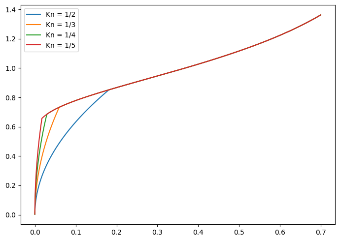
Refer to caption
Figure 1. Plot of t↦min⁡{|log⁡(C2​t)|−2​γ,Kn−γ/(s−s1)​t8​γ/(s−s1)}t\mapsto\min\{|\log(C_{2}t)|^{-2\gamma},K_{n}^{-\gamma/(s-s_{1})}t^{8\gamma/(s-s_{1})}\} for some values of the parameters and for variable KnK_{n}. For small tt, the behaviour of the modulus of continuity is Hölder, while for large tt it transitions to logarithmic. The scaling of the critical threshold t∗t_{*} is of order KnβK_{n}^{\beta} for some β>0\beta>0, up to log factors.

We highlight that the above result, in particular recovers the instability results from [ZZ19]. Indeed, relying on the more robust framework from [KRS21] in the form laid out in Sec. 4, we are able to relax the strong geometric assumptions from [ZZ19]. In particular, while in the setting of [ZZ19] it is assumed that

  • •

    σs​(x)=σs\sigma_{s}(x)=\sigma_{s} is independent of xx,

  • •

    D=B1​(0)D=B_{1}(0),

  • •

    σa∈𝒮:={σa∈L∞​(D):σa≥0,supp⁡(σa)⊂Br0​(0),σa∈Cq​(Br0​(0))}\sigma_{a}\in\mathcal{S}:=\{\sigma_{a}\in L^{\infty}(D):\ \sigma_{a}\geq 0,\ \operatorname{supp}(\sigma_{a})\subset B_{r_{0}}(0),\ \sigma_{a}\in C^{q}(B_{r_{0}}(0))\} for some r0∈(0,1)r_{0}\in(0,1), and q>0q>0,

in our instability framework we can investigate rather general geometries DD and compact sets K⋐DK\Subset D (which are not necessarily balls). This is a consequence of relying on more robust mapping properties which do not require symmetry conditions and, in particular, avoid the determination of explicit singular values and bases. As in [KRS21] we instead rely on compression properties which follow from the mapping properties of the forward operator.

1.2. Outline of the proof

In order to prove our main result (Theorem 1.1), we seek to use the abstract instability framework carried out in [KRS21]. We briefly outline the main ideas of the proof in what follows below.

Let X=L+∞​(D)X=L^{\infty}_{+}(D), let Y=ℬ​(Hs​(∂D),H−s​(∂D))Y=\mathcal{B}(H^{s}(\partial D),H^{-s}(\partial D)), where ss is as in Theorem 1.1, and let 𝒮⊂X\mathcal{S}\subset X be a compact set of absorption coefficients supported in K⋐DK\Subset D. We consider the forward operator

(1.5) Λ:X⟶Y\Lambda\colon X\longrightarrow Y

associated to the inverse problem, mapping σa∈L+∞​(D)\sigma_{a}\in L^{\infty}_{+}(D) to the corresponding albedo operator Λσa\Lambda_{\sigma_{a}} as defined in (2.3). A conditional stability estimate for the inverse problem, such as

(1.6) ‖σa,1−σa,2‖L∞​(D)≤ω​(‖Λσa,1−Λσa,2‖),σa,1,σa,2∈𝒮,\|\sigma_{a,1}-\sigma_{a,2}\|_{L^{\infty}(D)}\leq\omega(\|\Lambda_{\sigma_{a,1}}-\Lambda_{\sigma_{a,2}}\|),\quad\sigma_{a,1},\sigma_{a,2}\in\mathcal{S},

implies the following condition on the covering numbers of KK and of Λ​(𝒮)\Lambda(\mathcal{S}):

(1.7) 𝒩​(𝒮,ω​(ε),dX)≤𝒩​(Λ​(𝒮),ε,dY);\mathcal{N}(\mathcal{S},\omega(\varepsilon),d_{X})\leq\mathcal{N}(\Lambda(\mathcal{S}),\varepsilon,d_{Y});

we refer the reader to Sec. 4 for the definition and properties of covering numbers. Therefore, in order to prove a lower bound for ω=ω​(ε)\omega=\omega(\varepsilon) as in Theorem 1.1, it suffices to prove a lower bound for 𝒩​(𝒮,δ,dX)\mathcal{N}(\mathcal{S},\delta,d_{X}) and an upper bound for 𝒩​(Λ​(𝒮),ε,dY)\mathcal{N}(\Lambda(\mathcal{S}),\varepsilon,d_{Y}).

The lower bound for 𝒩​(𝒮,δ,dX)\mathcal{N}(\mathcal{S},\delta,d_{X}) comes from known entropy estimates for the embedding of Sobolev spaces into L∞​(D)L^{\infty}(D); see, for instance, [ET96] and Proposition 4.8. A crucial step in our proof is then to provide an upper bound for 𝒩​(Λ​(𝒮),ε,dY)\mathcal{N}(\Lambda(\mathcal{S}),\varepsilon,d_{Y}). In order to do this, we adopt the comparison strategy from [KRS21]: more precisely, we seek to derive an estimate of the following type (see Proposition 3.9)

(1.8) ‖(Λσa−Λ0)​f‖H−1/2​(∂D)≤C​(‖ρ0,0‖Hs0​(K)+Kn​‖f‖Hs1​(∂D)),σa∈𝒮,f∈Hs1​(∂D),\|(\Lambda_{\sigma_{a}}-\Lambda_{0})f\|_{H^{-1/2}(\partial D)}\leq C(\|\rho_{0,0}\|_{H^{s_{0}}(K)}+K_{n}\|f\|_{H^{s_{1}}(\partial D)}),\quad\sigma_{a}\in\mathcal{S},\ f\in H^{s_{1}}(\partial D),

where Λ0\Lambda_{0} is the albedo operator relative to the zero absorption coefficient, ρ0,0\rho_{0,0} is defined in Sec. 3, KnK_{n} is the Knudsen number and s0,s1>0s_{0},s_{1}>0. Roughly speaking, the structure of this estimate reflects the diffusion approximation of radiative transfer, namely the fact that a solution to the radiative transfer equation approaches a solution ρ0,0\rho_{0,0} to an elliptic boundary value problem (BVP) as Kn→0+K_{n}\rightarrow 0^{+}; the second terms accounts for a remainder that vanishes as Kn→0+K_{n}\rightarrow 0^{+}.

Equation (1.8) implies the existence of an orthonormal basis (fk)k(f_{k})_{k} of Hs​(∂D)H^{s}(\partial D) such that

‖(Λσa−Λ0)​fk‖H−1/2​(∂D)≤C​(exp⁡(−c​kμ)+Kn​k−ν),σa∈𝒮\displaystyle\|(\Lambda_{\sigma_{a}}-\Lambda_{0})f_{k}\|_{H^{-1/2}(\partial D)}\leq C(\exp(-ck^{\mu})+K_{n}k^{-\nu}),\quad\sigma_{a}\in\mathcal{S}

for some C,c,μ,ν>0C,c,\mu,\nu>0, which in turn implies the desired upper bound on 𝒩​(Λ​(𝒮),ε,dY)\mathcal{N}(\Lambda(\mathcal{S}),\varepsilon,d_{Y}) – see Sec. 4. The exponential decay in kk of the first term is related to the exponential instability of unique continuation for the solution of an elliptic equation from K⋐DK\Subset D to the boundary ∂D\partial D, while the power decay of the second term comes from entropy estimates for embeddings between Sobolev spaces.

We are then left to prove (1.8). In order to do this, we consider a test function g∈H1/2​(∂D)g\in H^{1/2}(\partial D) and its harmonic extension g~∈H1​(D)\tilde{g}\in H^{1}(D). The following formula holds (see Lemma 2.2):

(1.9) ⟨(Λσa−Λ0)​f,g⟩=−∫Dσa​⟨ua⟩​g~+1Kn​∫D⟨v​(ua−u0)⟩⋅∇g~.\langle(\Lambda_{\sigma_{a}}-\Lambda_{0})f,g\rangle=-\int_{D}\sigma_{a}\langle u_{a}\rangle\tilde{g}+\frac{1}{K_{n}}\int_{D}\langle v(u_{a}-u_{0})\rangle\cdot\nabla{\tilde{g}}.

Here, ⟨⋅,⋅⟩\langle\cdot,\cdot\rangle denotes the duality pairing between the respective Sobolev spaces on the left hand side. In this context, the functions uau_{a} and u0u_{0} solve (1.1) with absorption coefficients σa\sigma_{a} and 0, respectively, and boundary datum ff. The idea to obtain (1.8) is to plug in (1.9) the diffusion approximation expansion for both uau_{a} and u0u_{0}; the first terms in the expansion will be estimated by ‖ρ0,0‖Hs0​(K)\|\rho_{0,0}\|_{H^{s_{0}}(K)}, while the remainders will be estimated by Kn​‖f‖Hs1​(∂D)K_{n}\|f\|_{H^{s_{1}}(\partial D)}.

The diffusion approximation expansions to the first order for ua,u0u_{a},u_{0} are given by

ua∼ψa,0+ψa,1​Kn+ϕa,1​Kn,\displaystyle u_{a}\sim\psi_{a,0}+\psi_{a,1}K_{n}+\phi_{a,1}K_{n},
u0∼ψ0,0+ψ0,1​Kn+ϕ0,1​Kn,\displaystyle u_{0}\sim\psi_{0,0}+\psi_{0,1}K_{n}+\phi_{0,1}K_{n},

where ψa,0,ψa,1,ψ0,0,ψ0,1\psi_{a,0},\psi_{a,1},\psi_{0,0},\psi_{0,1} are referred to as interior solutions, while ϕa,1,ϕ0,1\phi_{a,1},\phi_{0,1} are referred to as boundary layer solutions – see, for instance, [BLP79, BdSS84]. The zeroth order boundary layers ϕa,0,ϕ0,0\phi_{a,0},\phi_{0,0} vanish due to the isotropic data ff. The zeroth order interior solutions ψa,0,ψ0,0\psi_{a,0},\psi_{0,0} coincide with the isotropic solutions ρa,0,ρ0,0\rho_{a,0},\rho_{0,0} to some elliptic BVP. In Sec. 3, we will define precisely the first terms in the diffusion approximation, show rigorously how to estimate them and how to deal with the remainder.

Although the construction of interior and boundary layers solutions outlined above is the classical approach to diffusion approximation expansions, the estimates concerning the higher order boundary layers require some care, as shown, for instance, in [WG14]. In order to avoid such technical issues, we adopt a different approach, already introduced in [DV25]: we write u=ua−u0u=u_{a}-u_{0} as

(1.10) u=ψ0+ψ1​Kn+Kn2​R,\displaystyle u=\psi_{0}+\psi_{1}K_{n}+K_{n}^{2}R,

where ψ0=ψa,0−ψ0,0\psi_{0}=\psi_{a,0}-\psi_{0,0}, ψ1=ψa,1−ψ1,0\psi_{1}=\psi_{a,1}-\psi_{1,0}, and estimate RR by studying the BVP it satisfies and leveraging estimates provided by the maximum principle for radiative transfer applied to specifically designed supersolutions. Using this strategy, we provide the following a priori estimates for the remainder RR from (1.10) and for the analogous error RaR_{a} in the diffusion approximation for uau_{a}.

Theorem 1.2.

Let K⋐DK\Subset D, let M>0M>0 and let σa∈𝒦\sigma_{a}\in\mathcal{K}, where 𝒦\mathcal{K} is defined as in (2.1). Then there exists C>0C>0 depending on D,K,MD,\ K,\ M and s0=3+⌊d2⌋,s1=92+⌊d2⌋s_{0}=3+\lfloor\frac{d}{2}\rfloor,\ s_{1}=\frac{9}{2}+\lfloor\frac{d}{2}\rfloor such that

(1.11) ‖⟨Ra⟩‖L∞​(D)≤C​(Kn−2​‖ρ0,0‖Hs0​(K)+Kn−1​‖f‖Hs1​(∂D)),\|\langle R_{a}\rangle\|_{L^{\infty}(D)}\leq C(K_{n}^{-2}\|\rho_{0,0}\|_{H^{s_{0}}(K)}+K_{n}^{-1}\|f\|_{H^{s_{1}}(\partial D)}),

and

(1.12) ‖⟨v​R⟩‖L∞​(D)≤C​(Kn−1​‖ρ0,0‖Hs0​(K)+‖f‖Hs1​(∂D)),\|\langle vR\rangle\|_{L^{\infty}(D)}\leq C(K_{n}^{-1}\|\rho_{0,0}\|_{H^{s_{0}}(K)}+\|f\|_{H^{s_{1}}(\partial D)}),

where RR, RaR_{a} and ρ0,0\rho_{0,0} are defined in Sec. 3 by (3.6), (3.5) and (3.1), respectively.

Both estimates are central in the estimates for our inverse problem. In particular, the proof of Theorem 1.2 will constitute the main technical part of the estimates on the diffusion approximation, and will be provided in Sec. 3.

1.3. Comparison with the literature

The study of the inverse problem for the radiative transfer equation is a classical theme with a large literature on it, see for instance [Bal09] for an overview. Uniqueness questions were addressed in the seminal works [CS96, CS99, SU23]. Building on these ideas, [Wan99] and [BJ08] investigated the associated stability properties for fixed Knudsen numbers. Relying on microlocal tools, a stability result in the critical regime of vanishing Knudsen numbers was derived in [LLU19]. Here the authors deduced a transition between a Hölder (for fixed Knudsen numbers) and a logarithmic (for increasingly small Knudsen numbers) stability regime.

A first indication of the optimality of this transition between a logarithmic and a Hölder regime was provided in [CLW18] in the linearized setting and confirmed in [ZZ19] in the full nonlinear regime (however with slightly different measurement operators than in [LLU19]). A key observation in these instability results is the proximity (in form of a diffusion approximation) of the nonlinear equation to the Calderón problem in the setting of small Knudsen numbers. Our work builds on these seminal contributions. It provides a robust framework for extending the available instability results to rather general geometries which do no longer require strong symmetry assumptions (such as spherical symmetry). Indeed, we work in an abstract framework similar as in [KRS21] adapted to our critical transition setting. This allows us to avoid the explicit computation of singular value bases but instead only requires good PDE bounds for the forward operator and for a suitable “comparison map”. We expect that this will also allow us to study variations and extensions of the above setting for this and related problems. Moreover, a key contribution of our work is also to provide precise quantitative estimates for the boundary behaviour of the remainder (see Theorem 1.2 and Sec. 3), which is fundamental to understand the contribution of first order terms in the diffusion expansion.

The diffusion approximation of the radiative transfer equation has been extensively studied both in the absence and in the presence of absorption, in the time-dependent case as well as in the stationary one. We refer to [BLP79, GW17, Wu21] for the diffusion approximation of the radiative transfer equation in the abscence of absorption-emission processes. The one-dimensional boundary layer equation has been studied for instance in [BdSS84] in the absence of absorption, in [Gol87] in the absence of scattering processes and in [Sen87] when both radiation processes are present. Finally, in [DV25] the diffusion approximation of the radiative transfer equation for the absorption-emission processes only has been studied through its formulation as a nonlocal integral equation via maximum principle arguments. This is the method that we will use also in this article. For further references concerning the study of the radiative transfer equation we refer to the PhD thesis [Dem25], which contains an exhaustive summary of the available literature.

1.4. Outline of the article

The remainder of the article is structured as follows. In Sec. 2, we introduce appropriate function spaces and recall some results about solutions for radiative transfer equations, together with the definition and some properties of the albedo operator in Subsec. 2.3. In Sec. 3, we provide a proof of the fine estimates for the diffusion approximation and for the remainder (see Theorem 1.2), and in Subsec. 3.7 we show how these imply the required estimates for the albedo operator. In Sec. 4, we prove our main result (Theorem 1.1) using the abstract framework from [KRS21] and the estimates provided later in the paper.

2. Preliminaries

In this section, we introduce appropriate function spaces and recall some results about solvability of radiative transfer equations.

2.1. Notation and function spaces

Let D⊂ℝdD\subset\mathbb{R}^{d} be a strictly convex, bounded domain with ∂D∈C5+⌊d2⌋\partial D\in C^{5+\lfloor\frac{d}{2}\rfloor},111This is the regularity of the boundary needed to derive the diffusion approximation estimates of Theorem 1.2; see Sec. 3. let Ω=Sd−1\Omega=S^{d-1} and let μ\mu denote the normalized (d−1)(d-1)-dimensional Hausdorff measure on Sd−1S^{d-1}. In the sequel, we will also consider a fixed compact set K⋐DK\Subset D and M>0M>0. We also introduce the spaces

L+∞​(D)\displaystyle L^{\infty}_{+}(D) ={σa∈L∞​(D):σa≥0}\displaystyle=\{\sigma_{a}\in L^{\infty}(D)\colon\ \sigma_{a}\geq 0\}

and the subset

(2.1) 𝒦={σa∈L+∞​(D):supp⁡(σa)⊂K,‖σa‖C2,1/2​(D)≤M}.\mathcal{K}=\{\sigma_{a}\in L^{\infty}_{+}(D)\colon\ \operatorname{supp}(\sigma_{a})\subset K,\ \|\sigma_{a}\|_{C^{2,1/2}(D)}\leq M\}.

Notice that, by Sobolev embedding, the set 𝒮\mathcal{S} defined in (1.2) is contained in 𝒦\mathcal{K}. We will often use the notation ‖σa‖𝒦\|\sigma_{a}\|_{\mathcal{K}} to denote the C2,1/2C^{2,1/2} norm of an element σa∈𝒦\sigma_{a}\in\mathcal{K}. Given a function u=u​(x,v)u=u(x,v), we will use the notation ⟨u⟩\langle u\rangle to denote the average in the velocity variable with respect to μ\mu. Unless otherwise noted, we use ∇\nabla to denote the gradient with respect to the space variables xx.

We define the anisotropic Sobolev space

W2​(D×Ω)={u∈𝒟′​(D×Ω):u∈L2​(D×Ω),v⋅∇u∈L2​(D×Ω)}.\displaystyle W^{2}(D\times\Omega)=\{u\in\mathcal{D}^{\prime}(D\times\Omega)\colon\,u\in L^{2}(D\times\Omega),\ v\cdot\nabla{u}\in L^{2}(D\times\Omega)\}.

This is a Hilbert space endowed with the inner product

(u1,u2)W2=(u1,u2)L2+(v⋅∇u1,v⋅∇u2)L2.\displaystyle(u_{1},u_{2})_{W^{2}}=(u_{1},u_{2})_{L^{2}}+(v\cdot\nabla{u_{1}},v\cdot\nabla{u_{2}})_{L^{2}}.

We define

Γ=∂D×Ω,\displaystyle\Gamma=\partial D\times\Omega,
Γ+={(x,v)∈Γ:v⋅nx>0},\displaystyle\Gamma_{+}=\{(x,v)\in\Gamma\colon\,v\cdot n_{x}>0\},
Γ−={(x,v)∈Γ:v⋅nx<0},\displaystyle\Gamma_{-}=\{(x,v)\in\Gamma\colon\,v\cdot n_{x}<0\},

and endow them with the measure

d​ξ=|v⋅nx|​d​x​d​μ​(v),\displaystyle d{\xi}=|v\cdot n_{x}|d{x}d\mu(v),

where d​xd{x} is the (d−1)(d-1)-dimensional Hausdorff measure on ∂D\partial D.

Theorem 2.1 (Traces in W2W^{2}).

There exist unique bounded operators

T±:W2​(D×Ω)→Lloc2​(Γ±,d​ξ)\displaystyle T_{\pm}\colon W^{2}(D\times\Omega)\rightarrow L^{2}_{\mathrm{loc}}(\Gamma_{\pm},d\xi)

that extend the operators T±​u=u|Γ±T_{\pm}u=u|_{\Gamma_{\pm}} defined on the dense subspace C∞​(D¯×Ω)⊂W2​(D×Ω)C^{\infty}(\overline{D}\times\Omega)\subset W^{2}(D\times\Omega).

Proof.

See [DL93, Ch. XXI, Sec. 2.2, Thm. 1]. ∎

We now define the following space

W∗2​(D×Ω)\displaystyle W^{2}_{*}(D\times\Omega) ={u∈W2​(D×Ω):u|Γ−∈L2​(Γ−,d​ξ)}.\displaystyle=\{u\in W^{2}(D\times\Omega)\colon\,u|_{\Gamma_{-}}\in L^{2}(\Gamma_{-},d\xi)\}.

This is a Hilbert space endowed with the inner product

(u1,u2)W∗2=(u1,u2)W2+(u1|Γ−,u2|Γ−)L2.\displaystyle(u_{1},u_{2})_{W^{2}_{*}}=(u_{1},u_{2})_{W^{2}}+(u_{1}|_{\Gamma_{-}},u_{2}|_{\Gamma_{-}})_{L^{2}}.
Theorem 2.2 (Traces in W∗2W_{*}^{2}).

The image of W∗2​(D×Ω)W^{2}_{*}(D\times\Omega) via the trace operator T+T_{+} is contained in L2​(Γ+,d​ξ)L^{2}(\Gamma_{+},d\xi). Moreover, the operator

T+:W∗2​(D×Ω)→L2​(Γ+,d​ξ)\displaystyle T_{+}\colon W_{*}^{2}(D\times\Omega)\rightarrow L^{2}(\Gamma_{+},d\xi)

is bounded.

Proof.

See [Bar70, Ces85]. ∎

Theorem 2.3 (Poincaré-Friedrichs inequality).

There exists a constant C=C​(D)>0C=C(D)>0 such that the following holds for u∈W∗2​(D×Ω)u\in W^{2}_{*}(D\times\Omega):

‖u‖L2​(D×Ω)≤C​(‖v⋅∇u‖L2​(D×Ω)+‖u|Γ−∥L2​(Γ−,d​ξ))\displaystyle\|u\|_{L^{2}(D\times\Omega)}\leq C\big(\|v\cdot\nabla{u}\|_{L^{2}(D\times\Omega)}+\|u|_{\Gamma_{-}}\|_{L^{2}(\Gamma_{-},d\xi)}\big)

In particular, the right hand side defines an equivalent norm on W∗2​(D×Ω)W^{2}_{*}(D\times\Omega).

Proof.

See [MRS00, Lemma 3.1]. ∎

2.2. Radiative transfer and the albedo operator

In this section, we recall some results about BVP for radiative transfer, and define the albedo operator.

Theorem 2.4.

Given σa∈L+∞​(D)\sigma_{a}\in L^{\infty}_{+}(D) with ‖σa‖L∞​(D)≤M\|\sigma_{a}\|_{L^{\infty}(D)}\leq M, F∈L2​(D×Ω)F\in L^{2}(D\times\Omega) and G∈L2​(Γ−,d​ξ)G\in L^{2}(\Gamma_{-},d{\xi}), there exists a unique (strong) solution u∈W∗2​(D×Ω)u\in W^{2}_{*}(D\times\Omega) of

(2.2) {v⋅∇u+Kn​σa​u+1Kn​(u−⟨u⟩)=Fin D×Ω,u|Γ−=G.\begin{cases}v\cdot\nabla{u}+K_{n}\sigma_{a}u+\frac{1}{K_{n}}(u-\langle u\rangle)=F&\text{in $D\times\Omega$},\\ u|_{\Gamma_{-}}=G.\end{cases}

Moreover, the following estimate holds for some C=C​(D,M)>0C=C(D,M)>0 and for Kn∈(0,1]K_{n}\in(0,1]:

‖u‖W∗2​(D×Ω)≤C​(Kn−1​‖F‖L2​(D×Ω)+Kn−1/2​‖G‖L2​(Γ−,d​ξ)).\displaystyle\|u\|_{W_{*}^{2}(D\times\Omega)}\leq C(K_{n}^{-1}\|F\|_{L^{2}(D\times\Omega)}+K_{n}^{-1/2}\|G\|_{L^{2}(\Gamma_{-},d{\xi})}).
Proof.

See [DL93, Ch. XXI, Sec. 4.1, Thm. 4], together with Remark 15 and Appendix 2 to Ch. XXI in the same reference, for a proof of existence and uniqueness. For the stability estimates, we first multiply (2.2) by uu and integrate over D×ΩD\times\Omega to obtain

12​∫D×Ωv⋅∇(u2)+Kn​∫D×Ωσa​u2+1Kn​∫D×Ω(u−⟨u⟩)​u\displaystyle\frac{1}{2}\int_{D\times\Omega}v\cdot\nabla(u^{2})+K_{n}\int_{D\times\Omega}\sigma_{a}u^{2}+\frac{1}{K_{n}}\int_{D\times\Omega}(u-\langle u\rangle)u =∫D×ΩF​u,\displaystyle=\int_{D\times\Omega}Fu,

and therefore

12​‖u‖L2​(Γ+,d​ξ)2−12​‖u‖L2​(Γ−,d​ξ)2+Kn​‖σa​u‖L2​(D×Ω)2+1Kn​‖u−⟨u⟩‖L2​(D×Ω)2\displaystyle\frac{1}{2}\|u\|_{L^{2}(\Gamma_{+},\mathrm{d}{\xi})}^{2}-\frac{1}{2}\|u\|_{L^{2}(\Gamma_{-},\mathrm{d}{\xi})}^{2}+K_{n}\|\sqrt{\sigma_{a}}u\|_{L^{2}(D\times\Omega)}^{2}+\frac{1}{K_{n}}\|u-\langle u\rangle\|_{L^{2}(D\times\Omega)}^{2} =(F,u)L2​(D×Ω),\displaystyle=(F,u)_{L^{2}(D\times\Omega)},

from which we deduce that

Kn​‖σa​u‖L2​(D×Ω)2+1Kn​‖u−⟨u⟩‖L2​(D×Ω)2≤|(F,u)L2​(D×Ω)|+12​‖G‖L2​(Γ−,d​ξ)2.\displaystyle K_{n}\|\sqrt{\sigma_{a}}u\|_{L^{2}(D\times\Omega)}^{2}+\frac{1}{K_{n}}\|u-\langle u\rangle\|_{L^{2}(D\times\Omega)}^{2}\leq|(F,u)_{L^{2}(D\times\Omega)}|+\frac{1}{2}\|G\|_{L^{2}(\Gamma_{-},\mathrm{d}{\xi})}^{2}.

We now use the equation for uu to estimate ‖v⋅∇u‖L2​(D×Ω)\|v\cdot\nabla{u}\|_{L^{2}(D\times\Omega)}:

‖v⋅∇u‖L2​(D×Ω)2\displaystyle\|v\cdot\nabla{u}\|_{L^{2}(D\times\Omega)}^{2} ≲Kn2​‖σa​u‖L2​(D×Ω)2+1Kn2​‖u−⟨u⟩‖L2​(D×Ω)2+‖F‖L2​(D×Ω)2\displaystyle\lesssim K_{n}^{2}\|\sigma_{a}u\|_{L^{2}(D\times\Omega)}^{2}+\frac{1}{K_{n}^{2}}\|u-\langle u\rangle\|_{L^{2}(D\times\Omega)}^{2}+\|F\|_{L^{2}(D\times\Omega)}^{2}
≤max⁡(M,1)Kn​(Kn​‖σa​u‖L2​(D×Ω)2+1Kn​‖u−⟨u⟩‖L2​(D×Ω)2)+‖F‖L2​(D×Ω)2\displaystyle\leq\frac{\max(M,1)}{K_{n}}\left(K_{n}\|\sqrt{\sigma_{a}}u\|_{L^{2}(D\times\Omega)}^{2}+\frac{1}{K_{n}}\|u-\langle u\rangle\|_{L^{2}(D\times\Omega)}^{2}\right)+\|F\|_{L^{2}(D\times\Omega)}^{2}
≲CεKn2​‖F‖L2​(D×Ω)2+ε​‖u‖L2​(D×Ω)2+1Kn​‖G‖L2​(Γ−,d​ξ)2.\displaystyle\lesssim\frac{C_{\varepsilon}}{K_{n}^{2}}\|F\|_{L^{2}(D\times\Omega)}^{2}+\varepsilon\|u\|_{L^{2}(D\times\Omega)}^{2}+\frac{1}{K_{n}}\|G\|_{L^{2}(\Gamma_{-},\mathrm{d}{\xi})}^{2}.

By Poincaré’s inequality (Theorem 2.3), we conclude that

‖u‖W∗2​(D×Ω)\displaystyle\|u\|_{W^{2}_{*}(D\times\Omega)} ≲‖v⋅∇u‖L2​(D×Ω)+‖G‖L2​(Γ−,d​ξ)\displaystyle\lesssim\|v\cdot\nabla{u}\|_{L^{2}(D\times\Omega)}+\|G\|_{L^{2}(\Gamma_{-},\mathrm{d}{\xi})}
≲Kn−1​‖F‖L2​(D×Ω)+ε​‖u‖L2​(D×Ω)+Kn−1/2​‖G‖L2​(Γ−,d​ξ).\displaystyle\lesssim K_{n}^{-1}\|F\|_{L^{2}(D\times\Omega)}+\varepsilon\|u\|_{L^{2}(D\times\Omega)}+K_{n}^{-1/2}\|G\|_{L^{2}(\Gamma_{-},\mathrm{d}{\xi})}.

Choosing ε\varepsilon sufficiently small implies the claim. ∎

2.3. Properties of the albedo operator

In this section, we deduce basic properties of the albedo operator. We begin by providing the strong form of the definition of the albedo operator which we will use in what follows below.

Definition 2.1.

Let s≥0s\geq 0 be fixed. Given σa∈L+∞​(D)\sigma_{a}\in L^{\infty}_{+}(D), we define the albedo operator Λσa∈ℬ​(Hs​(∂D),H−s​(∂D))\Lambda_{\sigma_{a}}\in\mathcal{B}(H^{s}(\partial D),H^{-s}(\partial D)) as follows: For f∈Hs​(∂D)f\in H^{s}(\partial D)

(2.3) Λσa​f=1Kn​∫Ω(v⋅nx)​ua|Γ​d​μ​(v)=1Kn​⟨(v⋅nx)​ua|Γ⟩,\Lambda_{\sigma_{a}}f=\frac{1}{K_{n}}\int_{\Omega}(v\cdot n_{x})u_{a}|_{\Gamma}\,d{\mu}(v)=\frac{1}{K_{n}}\langle(v\cdot n_{x})u_{a}|_{\Gamma}\rangle,

where ua∈W∗2​(D×Ω)u_{a}\in W^{2}_{*}(D\times\Omega) solves (2.2) with F=0F=0 and G=fG=f. We define the forward map

Λ:L+∞​(D)→ℬ​(Hs​(∂D),H−s​(∂D))\displaystyle\Lambda\colon L^{\infty}_{+}(D)\rightarrow\mathcal{B}(H^{s}(\partial D),H^{-s}(\partial D))

as Λ​(σa)=Λσa\Lambda(\sigma_{a})=\Lambda_{\sigma_{a}}.

We next provide a weak form of the albedo operator.

Lemma 2.2.

Let σa∈L+∞​(D)\sigma_{a}\in L^{\infty}_{+}(D), let f∈L2​(∂D)f\in L^{2}(\partial D) and let ua∈W∗2​(D×Ω)u_{a}\in W^{2}_{*}(D\times\Omega) be the solution of (2.2) with F=0F=0 and G=fG=f. Let g∈H1/2​(∂D)g\in H^{1/2}(\partial D) and let g~∈H1​(D)\tilde{g}\in H^{1}(D) be such that g~|∂D=g\tilde{g}|_{\partial D}=g. Then the following holds:

(2.4) ⟨Λσa​f,g⟩=−∫Dσa​⟨ua⟩​g~+1Kn​∫D⟨v​ua⟩⋅∇g~.\langle\Lambda_{\sigma_{a}}f,g\rangle=-\int_{D}\sigma_{a}\langle u_{a}\rangle\tilde{g}+\frac{1}{K_{n}}\int_{D}\langle vu_{a}\rangle\cdot\nabla{\tilde{g}}.
Proof.

Using the definition of Λσa\Lambda_{\sigma_{a}} and the divergence theorem, we have that

⟨Λσa​f,g⟩\displaystyle\langle\Lambda_{\sigma_{a}}f,g\rangle =1Kn​∫∂D⟨(v⋅nx)​ua⟩​g\displaystyle=\frac{1}{K_{n}}\int_{\partial D}\langle(v\cdot n_{x})u_{a}\rangle g
=1Kn​∫∂D⟨v​ua⟩​g⋅nx\displaystyle=\frac{1}{K_{n}}\int_{\partial D}\langle vu_{a}\rangle g\cdot n_{x}
=1Kn​∫D⟨v⋅∇ua⟩​g~+1Kn​∫D⟨v​ua⟩⋅∇g~.\displaystyle=\frac{1}{K_{n}}\int_{D}\langle v\cdot\nabla{u_{a}}\rangle\tilde{g}+\frac{1}{K_{n}}\int_{D}\langle vu_{a}\rangle\cdot\nabla\tilde{g}.

Using the equation satisfied by uau_{a} in the first term proves the lemma. ∎

For later use in the derivation of our instability estimates, we finally deduce the precise form of the Banach space adjoint operator Λσa′\Lambda_{\sigma_{a}}^{\prime} for the albedo operator. Here we make use of the isotropic boundary data under consideration.

Proposition 2.3.

Let f,g∈Hs​(∂D)f,g\in H^{s}(\partial D). Let ua∈W∗2​(D×Ω)u_{a}\in W_{*}^{2}(D\times\Omega) be the solution of (2.2) with F=0F=0 and G=fG=f, and let wa∈W∗2​(D×Ω)w_{a}\in W_{*}^{2}(D\times\Omega) be the solution of

(2.5) {−v⋅∇w+Kn​σa​w+1Kn​(w−⟨w⟩)=0in D×Ωw|Γ+=g.\begin{cases}-v\cdot\nabla{w}+K_{n}\sigma_{a}w+\frac{1}{K_{n}}(w-\langle w\rangle)=0&\text{in $D\times\Omega$}\\ w|_{\Gamma_{+}}=g.\end{cases}

Then the following holds:

⟨Λσa​f,g⟩=−1Kn​∫∂Df​⟨(v⋅nx)​wa⟩.\displaystyle\langle\Lambda_{\sigma_{a}}f,g\rangle=-\frac{1}{K_{n}}\int_{\partial D}f\langle(v\cdot n_{x})w_{a}\rangle.

In particular, we have that the adjoint operator Λσa′\Lambda_{\sigma_{a}}^{\prime} is given by

Λσa′​g=−1Kn​∫Ω(v⋅nx)​wa|Γ.\displaystyle\Lambda_{\sigma_{a}}^{\prime}g=-\frac{1}{K_{n}}\int_{\Omega}(v\cdot n_{x})w_{a}|_{\Gamma}.
Proof.

Integrating (2.2) (with F=0F=0) against waw_{a} on D×ΩD\times\Omega, we get

∫D×Ω(v⋅∇ua)​wa+Kn​∫D×Ωua​wa+1Kn​∫D×Ω(ua−⟨ua⟩)​wa=0.\displaystyle\int_{D\times\Omega}(v\cdot\nabla{u_{a}})w_{a}+K_{n}\int_{D\times\Omega}u_{a}w_{a}+\frac{1}{K_{n}}\int_{D\times\Omega}(u_{a}-\langle u_{a}\rangle)w_{a}=0.

The first term can be written as

∫D×Ω(v⋅∇ua)​wa=∫Γ(v⋅nx)​ua​wa−∫D×Ωua​(v⋅∇wa).\displaystyle\int_{D\times\Omega}(v\cdot\nabla{u_{a}})w_{a}=\int_{\Gamma}(v\cdot n_{x})u_{a}w_{a}-\int_{D\times\Omega}u_{a}(v\cdot\nabla w_{a}).

The last term can be written as

1Kn​∫D×Ω(ua−⟨ua⟩)​wa=1Kn​∫D×Ωua​(wa−⟨wa⟩).\displaystyle\frac{1}{K_{n}}\int_{D\times\Omega}(u_{a}-\langle u_{a}\rangle)w_{a}=\frac{1}{K_{n}}\int_{D\times\Omega}u_{a}(w_{a}-\langle w_{a}\rangle).

We conclude that

0\displaystyle 0 =∫Γ(v⋅nx)​ua​wa−∫D×Ωua​(v⋅∇wa)+Kn​∫D×Ωua​wa+1Kn​∫D×Ωua​(wa−⟨wa⟩)\displaystyle=\int_{\Gamma}(v\cdot n_{x})u_{a}w_{a}-\int_{D\times\Omega}u_{a}(v\cdot\nabla w_{a})+K_{n}\int_{D\times\Omega}u_{a}w_{a}+\frac{1}{K_{n}}\int_{D\times\Omega}u_{a}(w_{a}-\langle w_{a}\rangle)
=∫Γ(v⋅nx)​ua​wa,\displaystyle=\int_{\Gamma}(v\cdot n_{x})u_{a}w_{a},

where we have used the equation for waw_{a} in the last equality. Therefore, we have that

(2.6) ∫Γ+(v⋅nx)​ua​g=∫Γ+(v⋅nx)​ua​wa=−∫Γ−(v⋅nx)​ua​wa=−∫Γ−(v⋅nx)​f​wa.\int_{\Gamma_{+}}(v\cdot n_{x})u_{a}g=\int_{\Gamma_{+}}(v\cdot n_{x})u_{a}w_{a}=-\int_{\Gamma_{-}}(v\cdot n_{x})u_{a}w_{a}=-\int_{\Gamma_{-}}(v\cdot n_{x})fw_{a}.

Using the fact that f​gfg is isotropic, we infer that

∫Γ(v⋅nx)​f​g=0,\displaystyle\int_{\Gamma}(v\cdot n_{x})fg=0,

and therefore

(2.7) ∫Γ+(v⋅nx)​f​g=−∫Γ−(v⋅nx)​f​g.\int_{\Gamma_{+}}(v\cdot n_{x})fg=-\int_{\Gamma_{-}}(v\cdot n_{x})fg.

Adding (2.7) to (2.6), we deduce that

∫Γ(v⋅nx)​ua​g=−∫Γ(v⋅nx)​f​wa,\displaystyle\int_{\Gamma}(v\cdot n_{x})u_{a}g=-\int_{\Gamma}(v\cdot n_{x})fw_{a},

and we conclude. ∎

3. Diffusion approximation

In this section, we aim to prove Theorem 1.2. To this end, we will establish several estimates which can be obtained using the diffusion approximation. First of all we define the terms involved in the diffusion approximation. As we anticipated in the introduction, we consider the expansions

u0\displaystyle u_{0} =∑j=0∞Knj​ψ0,j​(x,v)=ψ0,0​(x,v)+Kn​ψ0,1​(x,v)+Kn2​R0​(x,v);\displaystyle=\sum_{j=0}^{\infty}K_{n}^{j}\psi_{0,j}(x,v)=\psi_{0,0}(x,v)+K_{n}\psi_{0,1}(x,v)+K_{n}^{2}R_{0}(x,v);
ua\displaystyle u_{a} =∑j=0∞Knj​ψa,j​(x,v)=ψa,0​(x,v)+Kn​ψa,1​(x,v)+Kn2​Ra​(x,v);\displaystyle=\sum_{j=0}^{\infty}K_{n}^{j}\psi_{a,j}(x,v)=\psi_{a,0}(x,v)+K_{n}\psi_{a,1}(x,v)+K_{n}^{2}R_{a}(x,v);
u\displaystyle u =ua−u0=∑j=0∞Knj​ψj​(x,v)=ψ0​(x,v)+Kn​ψ1​(x,v)+Kn2​R​(x,v).\displaystyle=u_{a}-u_{0}=\sum_{j=0}^{\infty}K_{n}^{j}\psi_{j}(x,v)=\psi_{0}(x,v)+K_{n}\psi_{1}(x,v)+K_{n}^{2}R(x,v).

We plug now these expressions into (1.1) and we compare the terms of the same order of magnitude. Therefore, we see that the zeroth order solutions ψa,0\psi_{a,0} and ψ0,0\psi_{0,0} are isotropic and satisfy ψa,0=ρa,0\psi_{a,0}=\rho_{a,0} and ψ0,0=ρ0,0\psi_{0,0}=\rho_{0,0}, where ρa,0,ρ0,0∈Hs0​(D)\rho_{a,0},\rho_{0,0}\in H^{s_{0}}(D) for s0=3+⌊d2⌋s_{0}=3+\lfloor\frac{d}{2}\rfloor are the solution to the following elliptic BVP:

(3.1) {−Cd​Δ​ρa,0+σa​ρa,0=0in D,ρa,0|∂D=f,{−Cd​Δ​ρ0,0=0in D,ρ0,0|∂D=f,\begin{cases}-C_{d}\Delta{\rho_{a,0}}+\sigma_{a}\rho_{a,0}=0&\text{in $D$},\\ \rho_{a,0}|_{\partial D}=f,\end{cases}\qquad\begin{cases}-C_{d}\Delta{\rho_{0,0}}=0&\text{in $D$},\\ \rho_{0,0}|_{\partial D}=f,\end{cases}

where Cd>0C_{d}>0 is such that ⟨v⊗v⟩=Cd​I\langle v\otimes v\rangle=C_{d}I and where f∈Hs1​(∂D)f\in H^{s_{1}}(\partial D) for s1=92+⌊d2⌋s_{1}=\frac{9}{2}+\lfloor\frac{d}{2}\rfloor. Notice, in particular, that ψ0=ψa,0−ψ0,0=ρa,0−ρ0,0\psi_{0}=\psi_{a,0}-\psi_{0,0}=\rho_{a,0}-\rho_{0,0} satisfies

(3.2) {−Cd​Δ​ψ0+σa​ψ0=−σa​ρ0,0in D,ψ0|∂D=0.\begin{cases}-C_{d}\Delta{\psi_{0}}+\sigma_{a}\psi_{0}=-\sigma_{a}\rho_{0,0}&\text{in $D$},\\ \psi_{0}|_{\partial D}=0.\end{cases}

We remark that, according to the method of matched asymptotic expansions, the boundary conditions of the problems (3.1) and (3.2) are determined by the limit as y→∞y\to\infty of the solutions to the boundary layer equations associated to the problems solved by the functions u0u_{0}, uau_{a} and uu, respectively. Indeed, the one-dimensional boundary layer equations are given at any point p∈∂Dp\in\partial D by

(3.3) {−(v⋅np)​∂yϕ​(y,v;p)=⟨ϕ⟩​(y;p)−ϕ​(y,v;p)y>0,v∈Sd−1,ϕa,0​(0,v;p)=g​(p)v⋅np<0,\begin{cases}-(v\cdot n_{p})\partial_{y}\phi(y,v;p)=\langle\phi\rangle(y;p)-\phi(y,v;p)&y>0,\;v\in S^{d-1},\\ \phi_{a,0}(0,v;p)=g(p)&v\cdot n_{p}<0,\end{cases}

where

g​(p)={f​(p) for the problem associated to ​u,ua,0 for the problem associated to ​u.g(p)=\begin{cases}f(p)&\text{ for the problem associated to }u,\ u_{a},\\ 0&\text{ for the problem associated to }u.\end{cases}

Since gg is isotropic, Theorem 4 in [BdSS84] implies that the unique bounded solution to (3.3) is given exactly by ϕ=g\phi=g.

The inverse of the operator

ϕ​(x,v)↦ϕ​(x,v)−⟨ϕ⟩​(x)\phi(x,v)\mapsto\phi(x,v)-\langle\phi\rangle(x)

is unique up to isotropic functions, therefore the first order terms are given by

ψ0,1​(x,v)=\displaystyle\psi_{0,1}(x,v)= −v⋅∇ρ0,0​(x)+c0​(x),\displaystyle-v\cdot\nabla\rho_{0,0}(x)+c_{0}(x),
ψa,1​(x,v)=\displaystyle\psi_{a,1}(x,v)= −v⋅∇ρa,0​(x)+ca​(x),\displaystyle-v\cdot\nabla\rho_{a,0}(x)+c_{a}(x),
ψ1​(x,v)=\displaystyle\psi_{1}(x,v)= −v⋅∇ψ0​(x)+c​(x),\displaystyle-v\cdot\nabla\psi_{0}(x)+c(x),

where c0c_{0}, cac_{a} and cc depend only on x∈Dx\in D.

First of all, we see that comparing the terms in the radiative transfer equation of order Kn2K_{n}^{2} these functions solve in the interior

−Cd​Δ​c0​(x)=0,−Cd​Δ​ca​(x)=−σa​ca​(x)​ and −Cd​Δ​c​(x)=−σa​(c0​(x)+c​(x)).\displaystyle-C_{d}\Delta c_{0}(x)=0,\quad-C_{d}\Delta c_{a}(x)=-\sigma_{a}c_{a}(x)\;\text{ and }\;-C_{d}\Delta c(x)=-\sigma_{a}(c_{0}(x)+c(x)).

The boundary conditions will be specified later and will be chosen in a specific way. Specifically, we will choose the functions c0,cac_{0},\ c_{a} and cc so that the contribution due to the boundary conditions of the remainders R0,RaR_{0},\ R_{a} and RR vanish in the interior of the domain. This is a key step for the proof of the estimates of Theorem 1.2.

With the definition of the zeroth and first order terms we see that the remainders R0R_{0}, RaR_{a} and RR solve (exactly) the following boundary value problems. The function R0R_{0} is a solution to

(3.4) {v⋅∇R0=1Kn​(⟨R0⟩−R0)+1Kn​(div​(v⊗v​∇ρ0,0)−v⋅∇c0)in ​D×ΩR0|Γ−=1Kn​(v⋅∇ρ0,0−c0)|Γ−.\begin{cases}v\cdot\nabla R_{0}=\frac{1}{K_{n}}\left(\langle R_{0}\rangle-R_{0}\right)+\frac{1}{K_{n}}\left(\mathrm{div}\left(v\otimes v\nabla\rho_{0,0}\right)-v\cdot\nabla c_{0}\right)&\text{in }D\times\Omega\\ \left.R_{0}\right|_{\Gamma_{-}}=\frac{1}{K_{n}}\left.\left(v\cdot\nabla\rho_{0,0}-c_{0}\right)\right|_{\Gamma_{-}}.\end{cases}

Notice that by construction ⟨div​(v⊗v​∇ρ0,0)−v⋅∇c0⟩=0\langle\mathrm{div}\left(v\otimes v\nabla\rho_{0,0}\right)-v\cdot\nabla c_{0}\rangle=0.

Similarly,

(3.5) {v⋅∇Ra=1Kn​(⟨Ra⟩−Ra)−Kn​σa​Ra+1Kn​(div​(v⊗v​∇ρa,0)−v⋅∇ca−σa​ρa,0)in ​D×Ω+σa​(v⋅∇ρa,0−ca)Ra|Γ−=1Kn​(v⋅∇ρa,0−ca)|Γ−\begin{cases}v\cdot\nabla R_{a}=\frac{1}{K_{n}}\left(\langle R_{a}\rangle-R_{a}\right)-K_{n}\sigma_{a}R_{a}\\ \qquad\qquad\qquad+\frac{1}{K_{n}}\left(\mathrm{div}\left(v\otimes v\nabla\rho_{a,0}\right)-v\cdot\nabla c_{a}-\sigma_{a}\rho_{a,0}\right)&\text{in }D\times\Omega\\ \qquad\qquad\qquad+\sigma_{a}\left(v\cdot\nabla\rho_{a,0}-c_{a}\right)\\ \left.R_{a}\right|_{\Gamma_{-}}=\frac{1}{K_{n}}\left.\left(v\cdot\nabla\rho_{a,0}-c_{a}\right)\right|_{\Gamma_{-}}\par\end{cases}

and

(3.6) {v⋅∇R=1Kn​(⟨R⟩−R)−Kn​σa​R+1Kn​(div​(v⊗v​∇ψ0)−v⋅∇c−σa​(ψ0+ρ0,0))+σa​(v⋅∇(ψ0+ρ0,0)−(c+c0))−Kn​σa​R0in ​D×ΩR|Γ−=1Kn​(v⋅∇ψ0−c)|Γ−.\begin{cases}v\cdot\nabla R=\frac{1}{K_{n}}\left(\langle R\rangle-R\right)-K_{n}\sigma_{a}R\\ \qquad\qquad\qquad+\frac{1}{K_{n}}\left(\mathrm{div}\left(v\otimes v\nabla\psi_{0}\right)-v\cdot\nabla c-\sigma_{a}\left(\psi_{0}+\rho_{0,0}\right)\right)\\ \qquad\qquad\qquad+\sigma_{a}\left(v\cdot\nabla\left(\psi_{0}+\rho_{0,0}\right)-\left(c+c_{0}\right)\right)-K_{n}\sigma_{a}R_{0}&\text{in }D\times\Omega\\ \left.R\right|_{\Gamma_{-}}=\frac{1}{K_{n}}\left.\left(v\cdot\nabla\psi_{0}-c\right)\right|_{\Gamma_{-}}.\end{cases}

According to Theorem 1.2 we aim to prove

|⟨Ra⟩​(x)|≤C​(D,σa,K)​‖ρ0,0‖Hs0​(D)Kn2+C​(D,σa,K)​‖f‖Hs1​(∂D)Kn\left|\langle R_{a}\rangle(x)\right|\leq C(D,\sigma_{a},K)\frac{\Arrowvert\rho_{0,0}\Arrowvert_{H^{s_{0}}(D)}}{K_{n}^{2}}+C(D,\sigma_{a},K)\frac{\Arrowvert f\Arrowvert_{H^{s_{1}}(\partial D)}}{K_{n}}

as well as

|⟨v​R⟩​(x)|≤C​(D,σa,K)​‖ρ0,0‖Hs0​(D)Kn+C​(D,σa,K)​‖f‖Hs1​(∂D).\left|\langle vR\rangle(x)\right|\leq C(D,\sigma_{a},K)\frac{\Arrowvert\rho_{0,0}\Arrowvert_{H^{s_{0}}(D)}}{K_{n}}+C(D,\sigma_{a},K)\Arrowvert f\Arrowvert_{H^{s_{1}}(\partial D)}.

Notice that, since Ra=R+R0R_{a}=R+R_{0}, it is enough to consider only R0R_{0} and RR.

Before proving rigorously these estimates, we first give some formal justification, why we expect such estimates to hold and how we expect the remainder to behave.

3.1. Formal discussion: The diffusion approximation

As Kn→0K_{n}\to 0 we expect by the diffusion approximation that the leading order of R0R_{0} and of RR solve in the bulk the following elliptic problems: For the leading order R0,0R_{0,0} of R0R_{0} we expect that it is a solution to

(3.7) −Cd​Δ​⟨R0,0⟩=⟨div​(v⊗v​∇div​(v⊗v​∇ρ0,0))⟩=0-C_{d}\Delta\langle R_{0,0}\rangle=\langle\mathrm{div}\left(v\otimes v\nabla\mathrm{div}\left(v\otimes v\nabla\rho_{0,0}\right)\right)\rangle=0

where we used that ⟨div​(v⊗v​∇div​(v⊗v​∇g​(x)))⟩=C¯d​Δ2​g​(x)\langle\mathrm{div}\left(v\otimes v\nabla\mathrm{div}\left(v\otimes v\nabla g(x)\right)\right)\rangle=\overline{C}_{d}\Delta^{2}g(x) and the properties of ρ0,0\rho_{0,0}.

Let R~0\tilde{R}_{0} denote the leading order of the remainder RR. We expect it to approximate in the bulk the solution of

(3.8) −Cd​Δ​⟨R~0⟩=−σa​⟨R~0⟩−σa​⟨R0,0⟩+C~d​Δ​(σa​(ψ0+ρ0,0,))−Cd​div​(σa​∇(ψ0+ρ0,0)),-C_{d}\Delta\langle\tilde{R}_{0}\rangle=-\sigma_{a}\langle\tilde{R}_{0}\rangle-\sigma_{a}\langle R_{0,0}\rangle+\tilde{C}_{d}\Delta\left(\sigma_{a}\left(\psi_{0}+\rho_{0,0,}\right)\right)-C_{d}\mathrm{div}\left(\sigma_{a}\nabla\left(\psi_{0}+\rho_{0,0}\right)\right),

where C~d=C¯dCd−Cd\tilde{C}_{d}=\frac{\overline{C}_{d}}{C_{d}}-C_{d}.

At this point it is worth to explain how the elliptic equations (3.7) and (3.8) are derived. Let us start considering R0=∑j≥0Knj​R0,jR_{0}=\sum_{j\geq 0}K_{n}^{j}R_{0,j}. Plugging this expansion into (3.4) and studying all terms of the same order of magnitude we see that

R0,0=⟨R0,0⟩+div​(v⊗v​∇ρ0,0)−v⋅∇c0,R_{0,0}=\langle R_{0,0}\rangle+\mathrm{div}\left(v\otimes v\nabla\rho_{0,0}\right)-v\cdot\nabla c_{0},

which is solvable since ⟨div​(v⊗v​∇ρ0,0)−v⋅∇c0⟩=0\langle\mathrm{div}\left(v\otimes v\nabla\rho_{0,0}\right)-v\cdot\nabla c_{0}\rangle=0. The first order terms give

v⋅∇R0,0=⟨R0,1⟩−R0,1v\cdot\nabla R_{0,0}=\langle R_{0,1}\rangle-R_{0,1}

which can be also solved since ⟨v⋅∇R0,0⟩=−Cd​Δ​c0=0\langle v\cdot\nabla R_{0,0}\rangle=-C_{d}\Delta c_{0}=0. Thus,

R0,1=⟨R0,1⟩−v⋅∇⟨R0,0⟩−v⋅∇div​(v⊗v​∇ρ0,0)−div​(v⊗v​∇c0).R_{0,1}=\langle R_{0,1}\rangle-v\cdot\nabla\langle R_{0,0}\rangle-v\cdot\nabla\mathrm{div}\left(v\otimes v\nabla\rho_{0,0}\right)-\mathrm{div}\left(v\otimes v\nabla c_{0}\right).

Finally, integrating the next order terms v⋅∇R0,1=⟨R0,2⟩−R0,2v\cdot\nabla R_{0,1}=\langle R_{0,2}\rangle-R_{0,2} over Sd−1S^{d-1} we obtain (3.7).

Moreover, near the boundary ∂D\partial D the behavior of R0R_{0} is given at the leading order by the solution of the following (1-dimensional) boundary layer equation defined for any p∈∂Dp\in\partial D

(3.9) {−(v⋅np)​∂yR¯0​(y,v;p)=⟨R¯0⟩−R¯0+div​(v⊗v​∇ρ0,0)|x=p−v⋅∇c0|x=py>0,v∈Sd−1,R¯0​(0,v;p)=1Kn​(v⋅∇ρ0,0−c0)|x=pv⋅np<0.\begin{cases}-(v\cdot n_{p})\partial_{y}\overline{R}_{0}(y,v;p)=\langle\overline{R}_{0}\rangle-\overline{R}_{0}+\mathrm{div}\left.\left(v\otimes v\nabla\rho_{0,0}\right)\right|_{x=p}-v\cdot\left.\nabla c_{0}\right|_{x=p}&y>0,\;v\in S^{d-1},\\ \overline{R}_{0}(0,v;p)=\frac{1}{K_{n}}\left.\left(v\cdot\nabla\rho_{0,0}-c_{0}\right)\right|_{x=p}&v\cdot n_{p}<0.\end{cases}

Thus, choosing c0|∂D\left.c_{0}\right|_{\partial D} to be such that limy→∞R¯0​(y,v;p)\lim\limits_{y\to\infty}\overline{R}_{0}(y,v;p) is bounded independently of KnK_{n} we can expect ⟨R0⟩\langle R_{0}\rangle, and thus also R0R_{0}, to be bounded in the bulk. Moreover, Theorem 4 in [BdSS84] and the linearity of the first equation in (3.9) will imply, as we will see later in a more rigorous way, that

|⟨R¯0⟩​(y,p)|≤C​(‖f‖)Kn​e−A​y+C​(‖f‖,‖ρ0,0‖),\left|\langle\overline{R}_{0}\rangle(y,p)\right|\leq\frac{C\left(\Arrowvert f\Arrowvert\right)}{K_{n}}e^{-Ay}+C\left(\Arrowvert f\Arrowvert,\Arrowvert\rho_{0,0}\Arrowvert\right),

so that we expect

(3.10) |⟨R0,0⟩​(x)|≤C​(‖f‖)Kn​e−A​d​(x)Kn+C​(‖f‖,‖ρ0,0‖),\left|\langle R_{0,0}\rangle(x)\right|\leq\frac{C\left(\Arrowvert f\Arrowvert\right)}{K_{n}}e^{-\frac{Ad(x)}{K_{n}}}+C\left(\Arrowvert f\Arrowvert,\Arrowvert\rho_{0,0}\Arrowvert\right),

where d​(x)=dist​(x,∂D)d(x)=\text{dist}(x,\partial D) and ∥⋅∥\|\cdot\| denotes some norms which are to be specified in what follows below. Notice that approximating the leading order of R0R_{0} using matched asymptotic expansions we can see that estimate (3.10) cannot be improved.

In a similar way we can argue for R=∑j≥0Knj​R~jR=\sum\limits_{j\geq 0}K_{n}^{j}\tilde{R}_{j} solving (3.6). The leading order satisfies

R~0=⟨R~0⟩+f1,\tilde{R}_{0}=\langle\tilde{R}_{0}\rangle+f_{1},

where f1=div​(v⊗v​∇ψ0)−v⋅∇c−σa​(ψ0+ρ0,0)f_{1}=\mathrm{div}\left(v\otimes v\nabla\psi_{0}\right)-v\cdot\nabla c-\sigma_{a}\left(\psi_{0}+\rho_{0,0}\right) with ⟨f1⟩=0\langle f_{1}\rangle=0. Since ⟨v⋅∇f1⟩=−Cd​Δ​c\langle v\cdot\nabla f_{1}\rangle=-C_{d}\Delta c and ⟨f2⟩=σa​(c+c0)\langle f_{2}\rangle=\sigma_{a}(c+c_{0}), where f2=−σa​(v⋅∇(ψ0+ρ0,0)−(c+c0))f_{2}=-\sigma_{a}\left(v\cdot\nabla\left(\psi_{0}+\rho_{0,0}\right)-\left(c+c_{0}\right)\right), we see that

R~1=⟨R~1⟩+f2−v⋅∇⟨R~0⟩−v⋅∇f1\tilde{R}_{1}=\langle\tilde{R}_{1}\rangle+f_{2}-v\cdot\nabla\langle\tilde{R}_{0}\rangle-v\cdot\nabla f_{1}

is solvable. Finally, we conclude that

v⋅∇R~1=⟨R~2⟩−R~2−σa​R~0−σa​R0,0.v\cdot\nabla\tilde{R}_{1}=\langle\tilde{R}_{2}\rangle-\tilde{R}_{2}-\sigma_{a}\tilde{R}_{0}-\sigma_{a}R_{0,0}.

Thus, integrating over Sd−1S^{d-1} we obtain (3.8). Notice that we used also

⟨div​(v⊗v​∇f1)⟩=C~d​Δ​(σa​(ψ0+ρ0,0))​ and ​⟨v⋅∇f2⟩=Cd​div​(σa​∇(ψ0+ρ0,0)).\displaystyle\langle\mathrm{div}\left(v\otimes v\nabla f_{1}\right)\rangle=\tilde{C}_{d}\Delta\left(\sigma_{a}(\psi_{0}+\rho_{0,0})\right)\;\text{ and }\;\langle v\cdot\nabla f_{2}\rangle=C_{d}\mathrm{div}\left(\sigma_{a}\nabla\left(\psi_{0}+\rho_{0,0}\right)\right).

Near the boundary ∂D\partial D the remainder RR behaves according to the boundary layer equation

(3.11) {−(v⋅np)​∂yR¯​(y,v;p)=⟨R¯⟩−R¯+f1​(v,p)y>0,v∈Sd−1,R¯​(0,v;p)=1Kn​(v⋅∇ψ0−c)|x=pv⋅np<0.\begin{cases}-(v\cdot n_{p})\partial_{y}\overline{R}(y,v;p)=\langle\overline{R}\rangle-\overline{R}+f_{1}(v,p)&y>0,\;v\in S^{d-1},\\ \overline{R}(0,v;p)=\frac{1}{K_{n}}\left.\left(v\cdot\nabla\psi_{0}-c\right)\right|_{x=p}&v\cdot n_{p}<0.\end{cases}

Once more we see that choosing in a proper way c|∂D\left.c\right|_{\partial D}

|⟨R¯⟩|≤C​(‖ψ0‖)Kn​ and ​limy→∞R¯​(y,v;p)​ is bounded,\left|\langle\overline{R}\rangle\right|\leq\frac{C(\Arrowvert\psi_{0}\Arrowvert)}{K_{n}}\text{ and }\lim\limits_{y\to\infty}\overline{R}(y,v;p)\text{ is bounded,}

where ∥⋅∥\Arrowvert\cdot\Arrowvert denotes some suitable norm that will be specified later. It is important also to notice that, while the bounds on the boundary layer solution R¯\overline{R} seem not to depend on ff, the elliptic equation (3.8) solved by the leading order in the bulk yields a bound of RR in terms of σa​R0\sigma_{a}R_{0}, among others. This is the reason why we will have to consider carefully the behaviour of R0R_{0}, especially near the boundary ∂D\partial D, where we expect the solution to explode as Kn→0K_{n}\rightarrow 0. This behaviour is substantiated by (formal) matched asymptotic expansions which yield the optimality of the estimate (3.10) (see also Proposition 3.5).

We remark also that because of the boundary layer equations we can expect neither R0R_{0} nor RR to be uniformly bounded in D¯\overline{D}. Due to the same reason, we can also not expect their LpL^{p}-norms to be bounded.

3.2. Construction of the auxiliary functions c0,cac_{0},\ c_{a} and cc

In this subsection we determine the function cc (respectively c0,cac_{0},\ c_{a}) such that the main contribution of the remainder RR (respectively R0,RaR_{0},\ R_{a}) is concentrated in a boundary layer of thickness KnK_{n} near the boundary.

As we introduced above, we set ψ0,1=−v⋅∇ρ0,0+c0\psi_{0,1}=-v\cdot\nabla\rho_{0,0}+c_{0} and ψ1=−v⋅∇ψ0+c\psi_{1}=-v\cdot\nabla\psi_{0}+c, where −Δ​c0=0-\Delta c_{0}=0 and −Cd​Δ​c=−σa​(c+c0)-C_{d}\Delta c=-\sigma_{a}(c+c_{0}) in the bulk. In this subsection we determine the boundary conditions that we should impose in order to guarantee that the solutions to the boundary layer equations (3.9) and (3.11) converge to a constant independent on KnK_{n} as y→∞y\to\infty. To this end, because of linearity, we consider the equation

{−(v⋅np)​∂yu​(y,v;p)=⟨u⟩−uy>0,v∈Sd−1,u​(0,v;p)=1Kn​(v⋅∇ϕ​(p)−a​(p))v⋅np<0\begin{cases}-(v\cdot n_{p})\partial_{y}u(y,v;p)=\langle u\rangle-u&y>0,\;v\in S^{d-1},\\ u(0,v;p)=\frac{1}{K_{n}}\left(v\cdot\nabla\phi(p)-a(p)\right)&v\cdot n_{p}<0\end{cases}

for some ∇ϕ∈C0​(D)\nabla\phi\in C^{0}(D) and some suitable function a​(p)a(p) to be determined below. Solving the ODE we obtain

u​(y,v;p)=\displaystyle u(y,v;p)= 1Kn​𝟙{v⋅np<0}​e−y|v⋅np|​(v⋅∇ϕ​(p)−a​(p))+𝟙{v⋅np<0}​(∫0ye−y−s|v⋅np||v⋅np|​⟨u⟩​(s;p)​𝑑s)\displaystyle\frac{1}{K_{n}}\mathbb{1}_{\{v\cdot n_{p}<0\}}e^{-\frac{y}{|v\cdot n_{p}|}}\left(v\cdot\nabla\phi(p)-a(p)\right)+\mathbb{1}_{\{v\cdot n_{p}<0\}}\left(\int_{0}^{y}\frac{e^{-\frac{y-s}{|v\cdot n_{p}|}}}{|v\cdot n_{p}|}\langle u\rangle(s;p)ds\right)
+𝟙{v⋅np>0}​(∫y∞ey−s|v⋅np||v⋅np|​⟨u⟩​(s;p)​𝑑s).\displaystyle+\mathbb{1}_{\{v\cdot n_{p}>0\}}\left(\int_{y}^{\infty}\frac{e^{\frac{y-s}{|v\cdot n_{p}|}}}{|v\cdot n_{p}|}\langle u\rangle(s;p)ds\right).

Integrating this expression over Sd−1S^{d-1} and using the symmetry properties of the function v↦𝟙{v⋅np<0}​e−y|v⋅np|​(v⋅τ)​(τ⋅∇ϕ​(p))v\mapsto\mathbb{1}_{\{v\cdot n_{p}<0\}}e^{-\frac{y}{|v\cdot n_{p}|}}(v\cdot\tau)(\tau\cdot\nabla\phi(p)), where τ⟂np\tau\perp n_{p}, we conclude that ⟨u⟩\langle u\rangle solves the following nonlocal equation

(3.12) ⟨u⟩​(y;p)−∫0∞E​(y−ξ)​⟨u⟩(ξ;p)​d​ξ=−1Kn​14​π​∫{v⋅np<0}[(v⋅np)​∂nϕ​(p)+a​(p)]​e−y|v⋅np|​𝑑v=12​Kn​[∂nϕ​(p)2​(e−y+y​e−y−y2​E1​(y))−a​(p)​(e−y−y​E1​(y))],\begin{split}\langle u\rangle(y;p)-\int_{0}^{\infty}E(y-\xi)\langle u\rangle&(\xi;p)d\xi=-\frac{1}{K_{n}}\frac{1}{4\pi}\int_{\{v\cdot n_{p}<0\}}\left[(v\cdot n_{p})\partial_{n}\phi(p)+a(p)\right]e^{-\frac{y}{|v\cdot n_{p}|}}dv\\ =&\frac{1}{2K_{n}}\left[\frac{\partial_{n}\phi(p)}{2}\left(e^{-y}+ye^{-y}-y^{2}E_{1}(y)\right)-a(p)\left(e^{-y}-yE_{1}(y)\right)\right],\end{split}

where E​(x)=E1​(x)2=12​∫|x|∞e−tt​𝑑tE(x)=\frac{E_{1}(x)}{2}=\frac{1}{2}\int_{|x|}^{\infty}\frac{e^{-t}}{t}dt is the normalized exponential integral. The nonlocal equation (3.12) has been obtained using a suitable change of variables as done in [DV25]. Moreover, we used also that

∫01e−ys​(1s)​𝑑s=(e−y−y​E1​(y)12​(e−y+y​e−y−y2​E1​(y))).\int_{0}^{1}e^{-\frac{y}{s}}\begin{pmatrix}1\\ s\end{pmatrix}ds=\begin{pmatrix}e^{-y}-yE_{1}(y)\\ \frac{1}{2}\left(e^{-y}+ye^{-y}-y^{2}E_{1}(y)\right)\end{pmatrix}.

Let us denote by ℒ\mathcal{L} the linear operator acting on L∞​(ℝ+)L^{\infty}(\mathbb{R}_{+}) defined as

(3.13) ℒ​(w)​(y)=w​(y)−∫0∞E​(y−ξ)​w​(ξ)​𝑑ξ.\mathcal{L}(w)(y)=w(y)-\int_{0}^{\infty}E(y-\xi)w(\xi)\ d\xi.

Since the sources are positive and have exponential decay, the results of Theorem 3.2, Theorem 3.3 and Lemma 3.4 in [DV25] imply the existence of unique non-negative continuous functions w1​(y)w_{1}(y), w2​(y)w_{2}(y) solving

ℒ​(w1)​(y)=12​(e−y+y​e−y−y2​E1​(y))andℒ​(w2)​(y)=e−y−y​E1​(y).\mathcal{L}(w_{1})(y)=\frac{1}{2}\left(e^{-y}+ye^{-y}-y^{2}E_{1}(y)\right)\qquad\text{and}\qquad\mathcal{L}(w_{2})(y)=e^{-y}-yE_{1}(y).

Moreover, there exist positive constants W1,W2>0W_{1},\ W_{2}>0 and C1,C2>0C_{1},\ C_{2}>0 such that

|w1​(y)−W1|≤C1​e−y2and|w2​(y)−W2|≤C2​e−y2.\left|w_{1}(y)-W_{1}\right|\leq C_{1}e^{-\frac{y}{2}}\qquad\text{and}\qquad\left|w_{2}(y)-W_{2}\right|\leq C_{2}e^{-\frac{y}{2}}.

Thus, defining for any p∈∂Dp\in\partial D

a​(p)=W1W2​∂nϕ​(p)a(p)=\frac{W_{1}}{W_{2}}\partial_{n}\phi(p)

we can conclude that ⟨u⟩​(y;p)\langle u\rangle(y;p) converges to zero as y→∞y\to\infty for every p∈∂Dp\in\partial D with exponential rate

|⟨u⟩​(y;p)|≤(C1+W1W2​C2)​|∂nϕ​(p)|2​Kn​e−y2.\left|\langle u\rangle(y;p)\right|\leq\left(C_{1}+\frac{W_{1}}{W_{2}}C_{2}\right)\frac{|\partial_{n}\phi(p)|}{2K_{n}}e^{-\frac{y}{2}}.

Hence, we define c0c_{0} and cc to be the solutions of the following Dirichlet problems

(3.14) {−Cd​Δ​c0=0 in ​D,c0|∂D=W1W2​∂nρ0,0|∂D,and{−Cd​Δ​c=−σa​(c+c0) in ​D,c|∂D=W1W2​∂nψ0|∂D.\begin{cases}-C_{d}\Delta c_{0}=0&\text{ in }D,\\ \left.c_{0}\right|_{\partial D}=\frac{W_{1}}{W_{2}}\left.\partial_{n}\rho_{0,0}\right|_{\partial D},\end{cases}\qquad\text{and}\qquad\begin{cases}-C_{d}\Delta c=-\sigma_{a}(c+c_{0})&\text{ in }D,\\ \left.c\right|_{\partial D}=\frac{W_{1}}{W_{2}}\left.\partial_{n}\psi_{0}\right|_{\partial D}.\end{cases}

In the following we will carry on the proof for Theorem 1.2 for the spacial dimension d=3d=3. Later, in Subsec. 3.6 we will generalize the result for any spacial dimension d≥3d\geq 3. Thus, we consider now s0=4s_{0}=4 and s1=5+12s_{1}=5+\frac{1}{2} as well as f∈Hs1​(∂D)f\in H^{s_{1}}(\partial D).

3.3. A rough estimate for the remainders

In this subsection we compute some first (rougher) estimates for the remainders RR and R0R_{0}, which are obtained mainly using in a straightforward way the triangle inequality. However, the resulting estimate for ⟨v​R⟩\langle vR\rangle turns out, as we will see, not to be the optimal one as stated in Theorem 1.2. We will show the following.

Lemma 3.1.

Let Kn∈(0,1]K_{n}\in(0,1]. The solution R∈L∞​(D×S2)R\in L^{\infty}(D\times S^{2}) of (3.6) satisfies the following bound

(3.15) |⟨R⟩​(x)|≤C1​(D,‖σa‖𝒦)​‖ρ0,0‖H4​(K)Kn+C2​(D,‖σa‖𝒦)​‖f‖Hs1​(∂D)+C3​(D)​‖σa​R0‖∞,\left|\langle R\rangle(x)\right|\leq C_{1}(D,\Arrowvert\sigma_{a}\Arrowvert_{\mathcal{K}})\frac{\|\rho_{0,0}\|_{H^{4}(K)}}{K_{n}}+C_{2}\left(D,\Arrowvert\sigma_{a}\Arrowvert_{\mathcal{K}}\right)\|f\|_{H^{s_{1}}(\partial D)}+C_{3}(D)\Arrowvert\sigma_{a}R_{0}\Arrowvert_{\infty},

where C1,C2,C3C_{1},\ C_{2},\ C_{3} are independent of KnK_{n}, C1C_{1} is independent of ff and C3C_{3} is a numerical constant independent on the data of the problem.

We will prove this lemma applying the maximum principle in a similar way as it has been done in Theorem 4.2. in [DV25]. Before giving the proof of Lemma 3.1, we need to derive a nonlocal equation solved by ⟨R⟩\langle R\rangle.

First of all, let us recall that f1=div​(v⊗v​∇ψ0)−v⋅∇c−σa​(ψ0+ρ0,0)f_{1}=\mathrm{div}\left(v\otimes v\nabla\psi_{0}\right)-v\cdot\nabla c-\sigma_{a}\left(\psi_{0}+\rho_{0,0}\right) and ⟨f2⟩=−σa​(c+c0)\langle f_{2}\rangle=-\sigma_{a}(c+c_{0}). Let also f3=σa​R0f_{3}=\sigma_{a}R_{0}. Then, by linearity, R=R0+R1+R2+R3R=R^{0}+R^{1}+R^{2}+R^{3}, where R0R^{0} solves

(3.16) {v⋅∇R0=1Kn​(⟨R0⟩−R0)−Kn​σa​R0in ​D×ΩR0|Γ−=1Kn​(v⋅∇ψ0−c)|Γ−\begin{cases}v\cdot\nabla R^{0}=\frac{1}{K_{n}}\left(\langle R^{0}\rangle-R^{0}\right)-K_{n}\sigma_{a}R^{0}&\text{in }D\times\Omega\\ \left.R^{0}\right|_{\Gamma_{-}}=\frac{1}{K_{n}}\left.\left(v\cdot\nabla\psi_{0}-c\right)\right|_{\Gamma_{-}}\end{cases}

and RiR^{i} solves for i∈{1,2,3}i\in\{1,2,3\}

(3.17) {v⋅∇Ri=1Kn​(⟨Ri⟩−Ri)−Kn​σa​R+Kni−2​fi​(x,v)in ​D×ΩRi|Γ−=0.\begin{cases}v\cdot\nabla R^{i}=\frac{1}{K_{n}}\left(\langle R^{i}\rangle-R^{i}\right)-K_{n}\sigma_{a}R+K_{n}^{i-2}f_{i}(x,v)&\text{in }D\times\Omega\\ \left.R^{i}\right|_{\Gamma_{-}}=0.\end{cases}

For any x∈Dx\in D and v∈Sd−1v\in S^{d-1}, let us define by y​(x,v)∈∂Dy(x,v)\in\partial D the unique intersection point of the half-line starting in xx and moving in direction −v-v with the boundary, i.e. y​(x,v)=∂D∩{x−t​v:t≥0}y(x,v)=\partial D\cap\left\{x-tv:t\geq 0\right\}. Moreover, we also define s​(x,v)=|x−y​(x,v)|s(x,v)=\left|x-y(x,v)\right|. Hence, solving by characteristics (3.16) and (3.17) yield

(3.18) R0​(x,v)=1Kn​(v⋅∇ψ0​(y​(x,v))−W1W2​∂nψ0​(y​(x,v)))​exp⁡(−∫0s​(x,v)1+Kn2​σa​(x−r​v)Kn​𝑑r)+∫0s​(x,v)1Kn​exp⁡(−∫0r1+Kn2​σa​(x−τ​v)Kn​𝑑τ)​⟨R0⟩​(x−r​v)​𝑑r\begin{split}R^{0}(x,v)=&\frac{1}{K_{n}}\left(v\cdot\nabla\psi_{0}(y(x,v))-\frac{W_{1}}{W_{2}}\partial_{n}\psi_{0}(y(x,v))\right)\exp\left(-\int_{0}^{s(x,v)}\frac{1+K_{n}^{2}\sigma_{a}(x-rv)}{K_{n}}\ dr\right)\\ &+\int_{0}^{s(x,v)}\frac{1}{K_{n}}\exp{\left(-\int_{0}^{r}\frac{1+K_{n}^{2}\sigma_{a}(x-\tau v)}{K_{n}}\ d\tau\right)}\langle R^{0}\rangle(x-rv)\ dr\end{split}

and for i∈{1,2,3}i\in\{1,2,3\}

(3.19) Ri​(x,v)=∫0s​(x,v)1Kn​exp⁡(−∫0r1+Kn2​σa​(x−τ​v)Kn​𝑑τ)​⟨R0⟩​(x−r​v)​𝑑r+∫0s​(x,v)Kni−2​exp⁡(−∫0r1+Kn2​σa​(x−τ​v)Kn​𝑑τ)​fi​(x−r​v,v)​𝑑r.\begin{split}R^{i}(x,v)=&\int_{0}^{s(x,v)}\frac{1}{K_{n}}\exp{\left(-\int_{0}^{r}\frac{1+K_{n}^{2}\sigma_{a}(x-\tau v)}{K_{n}}\ d\tau\right)}\langle R^{0}\rangle(x-rv)\ dr\\ &+\int_{0}^{s(x,v)}K_{n}^{i-2}\exp{\left(-\int_{0}^{r}\frac{1+K_{n}^{2}\sigma_{a}(x-\tau v)}{K_{n}}\ d\tau\right)}f_{i}(x-rv,v)\ dr.\end{split}

We remark that the considerations above, in particular equations (3.16), (3.17), (3.18) and (3.19) hold for any spacial dimension d≥3d\geq 3. Integrating now over S2S^{2} and using the change of variables (0,∞)×S2∋(r,v)↦η=x−r​v∈D(0,\infty)\times S^{2}\ni(r,v)\mapsto\eta=x-rv\in D we obtain, similarly as in [DV25], the following nonlocal equations solved by the averages in v∈S2v\in S^{2} of RiR^{i}

(3.20) ⟨R0⟩(x)−∫Dexp⁡(−∫[x,η]1+Kn2​σa​(ξ)Kn​𝑑ξ)4​π​Kn​|x−η|2⟨R0⟩(η)dη=14​π​Kn​∫S2(v⋅∇ψ0​(y​(x,v))−W1W2​∂nψ0​(y​(x,v)))​exp⁡(−∫0s​(x,v)1+Kn2​σa​(x−r​v)Kn​𝑑r)​𝑑v,\begin{split}\langle&R^{0}\rangle(x)-\int_{D}\frac{\exp{\left(-\int_{[x,\eta]}\frac{1+K_{n}^{2}\sigma_{a}(\xi)}{K_{n}}\ d\xi\right)}}{4\pi K_{n}|x-\eta|^{2}}\langle R^{0}\rangle(\eta)\ d\eta\\ =&\frac{1}{4\pi K_{n}}\int_{S^{2}}\left(v\cdot\nabla\psi_{0}(y(x,v))-\frac{W_{1}}{W_{2}}\partial_{n}\psi_{0}(y(x,v))\right)\exp\left(-\int_{0}^{s(x,v)}\frac{1+K_{n}^{2}\sigma_{a}(x-rv)}{K_{n}}\ dr\right)\ dv,\end{split}

where ∫[x,η]f​(ξ)​𝑑ξ=∫0|x−y|f​(x−t​x−y|x−y|)​𝑑t\int_{[x,\eta]}f(\xi)\ d\xi=\int_{0}^{|x-y|}f\left(x-t\frac{x-y}{|x-y|}\right)\ dt denotes the integral along the line connecting xx to η\eta. Moreover, for i∈{1,2,3}i\in\{1,2,3\} we have

(3.21) ⟨Ri⟩​(x)−∫Dexp⁡(−∫[x,η]1+Kn2​σa​(ξ)Kn​𝑑ξ)4​π​Kn​|x−η|2​⟨Ri⟩​(η)​𝑑η=Kni−24​π​∫S2∫0s​(x,v)exp⁡(−∫0r1+Kn2​σa​(x−τ​v)Kn​𝑑τ)​fi​(x−r​v,v)​𝑑r​𝑑v.\begin{split}\langle R^{i}\rangle(x)&-\int_{D}\frac{\exp{\left(-\int_{[x,\eta]}\frac{1+K_{n}^{2}\sigma_{a}(\xi)}{K_{n}}\ d\xi\right)}}{4\pi K_{n}|x-\eta|^{2}}\langle R^{i}\rangle(\eta)\ d\eta\\ =&\frac{K_{n}^{i-2}}{4\pi}\int_{S^{2}}\int_{0}^{s(x,v)}\exp\left(-\int_{0}^{r}\frac{1+K_{n}^{2}\sigma_{a}(x-\tau v)}{K_{n}}\ d\tau\right)f_{i}(x-rv,v)\ dr\ dv.\end{split}

In order to simplify the notation we define the kernel

EKn,σa​(x,η)=exp⁡(−∫[x,η]1+Kn2​σa​(ξ)Kn​𝑑ξ)4​π​Kn​|x−η|2E^{K_{n},\sigma_{a}}(x,\eta)=\frac{\exp{\left(-\int_{[x,\eta]}\frac{1+K_{n}^{2}\sigma_{a}(\xi)}{K_{n}}\ d\xi\right)}}{4\pi K_{n}|x-\eta|^{2}}

and the nonlocal operator

ℒDKn,σa​(u)​(x)=u​(x)−∫DEKn,σa​(x,η)​u​(η)​𝑑η.\mathcal{L}_{D}^{K_{n},\sigma_{a}}(u)(x)=u(x)-\int_{D}E^{K_{n},\sigma_{a}}(x,\eta)u(\eta)\ d\eta.

Notice that

(3.22) ∫ℝ3EKn,σa​(x,η)​dη=∫S2∫0s​(x,v)r2​EKn,σa​(x,x−r​v)​𝑑r​𝑑v≤∫S2∫0s​(x,v)r2​EKn,0​(x,x−r​v)​𝑑r​𝑑v≤∫0∞exp⁡(−rKn)Kn=1,\begin{split}\int_{\mathbb{R}^{3}}E^{K_{n},\sigma_{a}}(x,\eta)\,\mathrm{d}{\eta}&=\int_{S^{2}}\int_{0}^{s(x,v)}r^{2}E^{K_{n},\sigma_{a}}(x,x-rv)\ dr\ dv\\ &\leq\int_{S^{2}}\int_{0}^{s(x,v)}r^{2}E^{K_{n},0}(x,x-rv)\ dr\ dv\\ &\leq\int_{0}^{\infty}\frac{\exp\left(-\frac{r}{K_{n}}\right)}{K_{n}}=1,\end{split}

where we used σa≥0\sigma_{a}\geq 0. Thus, if ϕ≥0\phi\geq 0 then ℒDKn,σa​(ϕ)≥ℒDKn,0​(ϕ).\mathcal{L}_{D}^{K_{n},\sigma_{a}}(\phi)\geq\mathcal{L}_{D}^{K_{n},0}(\phi). We remark that ℒDKn,0\mathcal{L}_{D}^{K_{n},0} is the nonlocal operator considered in [DV25]. As in [DV25], the Banach fixed-point theorem guarantees the existence of unique solutions ⟨Ri⟩∈L∞​(D)\langle R^{i}\rangle\in L^{\infty}(D) for all i∈{0,1,2,3}i\in\{0,1,2,3\}. In addition to that, due to the regularity assumptions on σa\sigma_{a} and on ff the solution ⟨Ri⟩\langle R^{i}\rangle is continuous. Moreover, for any σa≥0\sigma_{a}\geq 0 the operator ℒDKn,σa\mathcal{L}_{D}^{K_{n},\sigma_{a}} satisfies the following global maximum principle.

Proposition 3.2.

Let u∈C​(D¯)u\in C(\overline{D}). Assume that uu satisfies one of the following assumptions

  1. (1)

    ℒDKn,σa​(u)​(x)≥0\mathcal{L}_{D}^{K_{n},\sigma_{a}}(u)(x)\geq 0 for all x∈Dx\in D,

  2. (2)

    ℒDKn,σa​(u)​(x)≥0\mathcal{L}_{D}^{K_{n},\sigma_{a}}(u)(x)\geq 0 for all x∈O⊂Dx\in O\subset D open and u≥0u\geq 0 in D∖OD\setminus O.

Then u≥0u\geq 0 in DD.

Proof.

Assume that there exists y∈D¯y\in\overline{D} such that minD¯⁡u=u​(y)<0\min\limits_{\overline{D}}u=u(y)<0. Then using the property (3.22) the following contradiction arises

0≤ℒDKn,σa​(u)​(y)≤u​(y)​∫DcEKn,σa​(y,η)​𝑑η+∫DEKn,σa​(y,η)​(u​(y)−u​(η))​𝑑η<0.0\leq\mathcal{L}_{D}^{K_{n},\sigma_{a}}(u)(y)\leq u(y)\int_{D^{c}}E^{K_{n},\sigma_{a}}(y,\eta)d\eta+\int_{D}E^{K_{n},\sigma_{a}}(y,\eta)\left(u(y)-u(\eta)\right)d\eta<0.

∎

The property ℒDKn,σa​[ϕ]≥ℒDKn,0​[ϕ]\mathcal{L}_{D}^{K_{n},\sigma_{a}}[\phi]\geq\mathcal{L}_{D}^{K_{n},0}[\phi] for ϕ≥0\phi\geq 0 implies that the supersolutions constructed in [DV25] are supersolutions also for the operator ℒDKn,σa\mathcal{L}_{D}^{K_{n},\sigma_{a}} for σa≢0\sigma_{a}\not\equiv 0. In particular, the function given in Lemma 4.1 of [DV25] given by

(3.23) ϕKn1​(x)=CD−|x|2,\phi_{K_{n}}^{1}(x)=C_{D}-|x|^{2},

where CD=2​maxD¯⁡|x|2+2​(diam​(D))2+4​diam​(D)+4C_{D}=2\max\limits_{\overline{D}}|x|^{2}+2\left(\text{diam}(D)\right)^{2}+4\text{diam}(D)+4, satisfies

ℒDKn,σa​[ϕKn1]≥2​Kn2.\mathcal{L}_{D}^{K_{n},\sigma_{a}}\left[\phi_{K_{n}}^{1}\right]\geq 2K_{n}^{2}.

Moreover, consider the function

(3.24) ϕKn,A2​(x)=C1​(D)​ϕKn1​(x)+C2​(D)​[(1−γ1+(d​(x)A​Kn)2)∧(1−γ1+(μ​RA​Kn)2)]\phi_{K_{n},A}^{2}(x)=C_{1}(D)\phi_{K_{n}}^{1}(x)+C_{2}(D)\left[\left(1-\frac{\gamma}{1+\left(\frac{d(x)}{AK_{n}}\right)^{2}}\right)\wedge\left(1-\frac{\gamma}{1+\left(\frac{\mu R}{AK_{n}}\right)^{2}}\right)\right]

defined in Theorem 4.2 of [DV25] for A≥1A\geq 1, suitable γ,μ∈(0,1)\gamma,\mu\in(0,1) and suitable constants C1​(D)C_{1}(D) and C2​(D)C_{2}(D) which depend only on the domain DD whose minimal radius of curvature is denoted by R=min∂D⁡R​(x)R=\min\limits_{\partial D}R(x). Then, also in this case we have

ℒDKn,σa​[ϕKn,A2]≥e−d​(x)A​Kn.\mathcal{L}_{D}^{K_{n},\sigma_{a}}\left[\phi_{K_{n},A}^{2}\right]\geq e^{-\frac{d(x)}{AK_{n}}}.

We are now ready to prove Lemma 3.1.

Proof of Lemma 3.1.

Let f∈H5+12​(∂D)f\in H^{5+\frac{1}{2}}(\partial D). Then there exists an extension f~∈H6​(D)\tilde{f}\in H^{6}(D) such that f~=f\tilde{f}=f in ∂D\partial D in the trace sense. Thus, elliptic Sobolev regularity implies that ρ0,0∈H6​(D)\rho_{0,0}\in H^{6}(D). By the Sobolev embedding we conclude also that ρ0,0∈C4,12\rho_{0,0}\in C^{4,\frac{1}{2}}. Thus, by Schauder theory we obtain that ψ0∈C6,12​(D)\psi_{0}\in C^{6,\frac{1}{2}}(D) and it satisfies

(3.25) ‖D4​ψ0‖∞≤‖σa​ρ0,0‖C2,12​(D)≤‖σa‖𝒦​‖ρ0,0‖H4​(K)\Arrowvert D^{4}\psi_{0}\Arrowvert_{\infty}\leq\Arrowvert\sigma_{a}\rho_{0,0}\Arrowvert_{C^{2,\frac{1}{2}}(D)}\leq\Arrowvert\sigma_{a}\Arrowvert_{\mathcal{K}}\Arrowvert\rho_{0,0}\Arrowvert_{H^{4}(K)}

as well as

(3.26) ‖D2​ψ0‖∞≤‖σa​ρ0,0‖C0,12​(D)≤‖σa‖𝒦​‖ρ0,0‖H2​(K).\Arrowvert D^{2}\psi_{0}\Arrowvert_{\infty}\leq\Arrowvert\sigma_{a}\rho_{0,0}\Arrowvert_{C^{0,\frac{1}{2}}(D)}\leq\Arrowvert\sigma_{a}\Arrowvert_{\mathcal{K}}\Arrowvert\rho_{0,0}\Arrowvert_{H^{2}(K)}.

Moreover, c,c0∈C3,12​(D)c,c_{0}\in C^{3,\frac{1}{2}}(D) and satisfy

(3.27) ‖c‖C3,12​(D)≤‖σa‖𝒦​‖ρ0,0‖H4​(K)+‖σa‖𝒦​‖f‖H5+12​(∂D),\Arrowvert c\Arrowvert_{C^{3,\frac{1}{2}}(D)}\leq\Arrowvert\sigma_{a}\Arrowvert_{\mathcal{K}}\Arrowvert\rho_{0,0}\Arrowvert_{H^{4}(K)}+\Arrowvert\sigma_{a}\Arrowvert_{\mathcal{K}}\Arrowvert f\Arrowvert_{H^{5+\frac{1}{2}}(\partial D)},
(3.28) ‖c‖C1,12​(D)≤‖σa‖𝒦​‖ρ0,0‖H2​(K)+‖σa‖𝒦​‖f‖H5+12​(∂D),\Arrowvert c\Arrowvert_{C^{1,\frac{1}{2}}(D)}\leq\Arrowvert\sigma_{a}\Arrowvert_{\mathcal{K}}\Arrowvert\rho_{0,0}\Arrowvert_{H^{2}(K)}+\Arrowvert\sigma_{a}\Arrowvert_{\mathcal{K}}\Arrowvert f\Arrowvert_{H^{5+\frac{1}{2}}(\partial D)},

and

(3.29) ‖c0‖C3,12​(D)≤‖f‖H5+12​(∂D).\Arrowvert c_{0}\Arrowvert_{C^{3,\frac{1}{2}}(D)}\leq\Arrowvert f\Arrowvert_{H^{5+\frac{1}{2}}(\partial D)}.

Let us consider first |⟨R0⟩||\langle R^{0}\rangle|. Since ψ0|∂D=0\left.\psi_{0}\right|_{\partial D}=0 we can estimate

|ℒDKn,σa​[⟨R0⟩]​(x)|≤14​π​Kn​|∫S2(v⋅ny​(x,v)−W1W2)​∂nψ0​(y​(x,v))​exp⁡(−∫0s​(x,v)1+Kn2​σa​(x−r​v)Kn​𝑑r)​d​v|≤(1+W1W2)​‖σa‖𝒦​‖ρ0,0‖H2​(K)Kn​e−d​(x)Kn.\begin{split}&\bigg|\mathcal{L}_{D}^{K_{n},\sigma_{a}}[\langle R^{0}\rangle](x)\bigg|\\ &\leq\frac{1}{4\pi K_{n}}\left|\int_{S^{2}}\left(v\cdot n_{y(x,v)}-\frac{W_{1}}{W_{2}}\right)\partial_{n}\psi_{0}(y(x,v))\exp\left(-\int_{0}^{s(x,v)}\frac{1+K_{n}^{2}\sigma_{a}(x-rv)}{K_{n}}\ dr\right)\ dv\right|\\ &\leq\left(1+\frac{W_{1}}{W_{2}}\right)\frac{\Arrowvert\sigma_{a}\Arrowvert_{\mathcal{K}}\Arrowvert\rho_{0,0}\Arrowvert_{H^{2}(K)}}{K_{n}}e^{-\frac{d(x)}{K_{n}}}.\end{split}

Therefore, an application of the maximum principle stated in Proposition 3.2 with the supersolution A​ϕKn,12A\phi_{K_{n},1}^{2} (for a suitable constant A>0A>0 independent of KnK_{n}) implies

|⟨R0⟩​(x)|≤C​(D)​‖σa‖𝒦​‖ρ0,0‖H2​(K)Kn.\left|\langle R^{0}\rangle(x)\right|\leq C(D)\Arrowvert\sigma_{a}\Arrowvert_{\mathcal{K}}\frac{\Arrowvert\rho_{0,0}\Arrowvert_{H^{2}(K)}}{K_{n}}.

Next we consider ⟨R1+R2⟩\langle R^{1}+R^{2}\rangle. To this end we consider the Taylor expansions

(3.30) f1​(x−r​v,v)=f1​(x,v)−r​v⋅∇f1​(x,v)+r22​vT​∇x2f1​(x,v)​v+𝒪​(|r​v|2​‖D2​f1‖∞)f_{1}(x-rv,v)=f_{1}(x,v)-rv\cdot\nabla f_{1}(x,v)+\frac{r^{2}}{2}v^{T}\nabla^{2}_{x}f_{1}(x,v)v+\mathcal{O}\left(|rv|^{2}\Arrowvert D^{2}f_{1}\Arrowvert_{\infty}\right)

and

(3.31) f2​(x−r​v,v)=f2​(x,v)−r​v⋅∇f2​(x,v)+𝒪​(|r​v|​‖D​f2‖∞),f_{2}(x-rv,v)=f_{2}(x,v)-rv\cdot\nabla f_{2}(x,v)+\mathcal{O}\left(|rv|\Arrowvert Df_{2}\Arrowvert_{\infty}\right),

where by definition

‖D2​f1‖∞≤C​(‖σa‖𝒦)​(‖ρ0,0‖H4​(K)+‖f‖H5+12​(∂D)),\displaystyle\Arrowvert D^{2}f_{1}\Arrowvert_{\infty}\leq C(\Arrowvert\sigma_{a}\Arrowvert_{\mathcal{K}})(\|\rho_{0,0}\|_{H^{4}(K)}+\Arrowvert f\Arrowvert_{H^{5+\frac{1}{2}}(\partial D)}),
‖D​f2‖∞≤C​(‖σa‖𝒦)​(‖ρ0,0‖H4​(K)+‖f‖H5+12​(∂D)).\displaystyle\Arrowvert Df_{2}\Arrowvert_{\infty}\leq C(\Arrowvert\sigma_{a}\Arrowvert_{\mathcal{K}})(\|\rho_{0,0}\|_{H^{4}(K)}+\Arrowvert f\Arrowvert_{H^{5+\frac{1}{2}}(\partial D)}).

Moreover, we will use that ⟨f1⟩=0\langle f_{1}\rangle=0 and that ⟨v⋅∇f1⟩=−Cd​Δ​c=−σa​(c+c0)=⟨f2⟩\langle v\cdot\nabla f_{1}\rangle=-C_{d}\Delta c=-\sigma_{a}(c+c_{0})=\langle f_{2}\rangle. The next results are also helpful for the estimate of ℒDKn,σa​[⟨R1+R2⟩]\mathcal{L}_{D}^{K_{n},\sigma_{a}}\left[\langle R^{1}+R^{2}\rangle\right].

∫0s​(x,v)exp⁡(−∫0r1+Kn2​σa​(x−τ​v)Kn​𝑑τ)​𝑑r=\displaystyle\int_{0}^{s(x,v)}\exp{\left(-\int_{0}^{r}\frac{1+K_{n}^{2}\sigma_{a}(x-\tau v)}{K_{n}}\ d\tau\right)}\ dr= Kn1+Kn2​σa\displaystyle\frac{K_{n}}{1+K_{n}^{2}\sigma_{a}}
+𝒪​(Kn​e−d​(x)Kn+Kn3​‖∇σa‖∞​(1−e−d​(x)Kn)),\displaystyle+\mathcal{O}\left(K_{n}e^{-\frac{d(x)}{K_{n}}}+K_{n}^{3}\Arrowvert\nabla\sigma_{a}\Arrowvert_{\infty}\left(1-e^{-\frac{d(x)}{K_{n}}}\right)\right),
∫0s​(x,v)r​exp⁡(−∫0r1+Kn2​σa​(x−τ​v)Kn​𝑑τ)​𝑑r=\displaystyle\int_{0}^{s(x,v)}r\exp{\left(-\int_{0}^{r}\frac{1+K_{n}^{2}\sigma_{a}(x-\tau v)}{K_{n}}\ d\tau\right)}\ dr= Kn2(1+Kn2​σa)2\displaystyle\frac{K_{n}^{2}}{\left(1+K_{n}^{2}\sigma_{a}\right)^{2}}
+𝒪​(Kn2​e−d​(x)2​Kn+Kn4​‖∇σa‖∞​(1−e−d​(x)2​Kn)),\displaystyle+\mathcal{O}\left(K_{n}^{2}e^{-\frac{d(x)}{2K_{n}}}+K_{n}^{4}\Arrowvert\nabla\sigma_{a}\Arrowvert_{\infty}\left(1-e^{-\frac{d(x)}{2K_{n}}}\right)\right),
∫0s​(x,v)r2​exp⁡(−∫0r1+Kn2​σa​(x−τ​v)Kn​𝑑τ)​𝑑r=\displaystyle\int_{0}^{s(x,v)}r^{2}\exp{\left(-\int_{0}^{r}\frac{1+K_{n}^{2}\sigma_{a}(x-\tau v)}{K_{n}}\ d\tau\right)}\ dr= 2​Kn3(1+Kn2​σa)3\displaystyle\frac{2K_{n}^{3}}{\left(1+K_{n}^{2}\sigma_{a}\right)^{3}}
+𝒪​(Kn3​e−d​(x)2​Kn+Kn5​‖∇σa‖∞​(1−e−d​(x)2​Kn)).\displaystyle+\mathcal{O}\left(K_{n}^{3}e^{-\frac{d(x)}{2K_{n}}}+K_{n}^{5}\Arrowvert\nabla\sigma_{a}\Arrowvert_{\infty}\left(1-e^{-\frac{d(x)}{2K_{n}}}\right)\right).

Thus,

|ℒDKn,σa[⟨R1+R2⟩](x)|≤Kn3(1+Kn2​σa)2∥σa2(c+c0)∥∞+C​(‖σa‖𝒦​(‖ρ0,0‖H2​(K)+‖f‖H5+12​(∂D)))​(e−d​(x)2​Kn+Kn2(1+Kn2​σa)2+Kn2​‖∇σa‖∞​(1−e−d​(x)2​Kn)).\begin{split}\bigg|&\mathcal{L}_{D}^{K_{n},\sigma_{a}}\left[\langle R^{1}+R^{2}\rangle\right](x)\bigg|\leq\frac{K_{n}^{3}}{\left(1+K_{n}^{2}\sigma_{a}\right)^{2}}\Arrowvert\sigma_{a}^{2}(c+c_{0})\Arrowvert_{\infty}\\ &+C\left(\Arrowvert\sigma_{a}\Arrowvert_{\mathcal{K}}\left(\Arrowvert\rho_{0,0}\Arrowvert_{H^{2}(K)}+\Arrowvert f\Arrowvert_{H^{5+\frac{1}{2}}(\partial D)}\right)\right)\left(e^{-\frac{d(x)}{2K_{n}}}+\frac{K_{n}^{2}}{\left(1+K_{n}^{2}\sigma_{a}\right)^{2}}+K_{n}^{2}\Arrowvert\nabla\sigma_{a}\Arrowvert_{\infty}\left(1-e^{-\frac{d(x)}{2K_{n}}}\right)\right).\end{split}

An application of the maximum principle (with A​ϕKn1A\phi^{1}_{K_{n}} for a suitable constant A>0A>0) stated in Proposition 3.2 implies that

|⟨R1+R2⟩​(x)|≤C​(D,‖σa‖𝒦)​(‖ρ0,0‖H4​(K)+‖f‖H5+12​(∂D)).\left|\langle R^{1}+R^{2}\rangle(x)\right|\leq C\left(D,\Arrowvert\sigma_{a}\Arrowvert_{\mathcal{K}}\right)\left(\Arrowvert\rho_{0,0}\Arrowvert_{H^{4}(K)}+\Arrowvert f\Arrowvert_{H^{5+\frac{1}{2}}(\partial D)}\right).

Finally, we estimate the term |⟨R3⟩|\left|\langle R^{3}\rangle\right| in the following way

|ℒDKn,σa​[⟨R3⟩]​(x)|≤|Kn4​π​∫S2∫0s​(x,v)exp⁡(−∫0r1+Kn2​σa​(x−τ​v)Kn​𝑑τ)​σa​(x−r​v)​R0​(x−r​v,v)​𝑑r​𝑑v|≤Kn​‖σa​R0‖∞​|14​π​∫S2∫0s​(x,v)e−rKn​𝑑r​𝑑v|≤Kn2​‖σa​R0‖∞​(1−e−d​(x)Kn).\begin{split}\bigg|&\mathcal{L}_{D}^{K_{n},\sigma_{a}}\left[\langle R^{3}\rangle\right](x)\bigg|\leq\\ &\left|\frac{K_{n}}{4\pi}\int_{S^{2}}\int_{0}^{s(x,v)}\exp\left(-\int_{0}^{r}\frac{1+K_{n}^{2}\sigma_{a}(x-\tau v)}{K_{n}}\ d\tau\right)\sigma_{a}(x-rv)R_{0}(x-rv,v)\ dr\ dv\right|\\ &\leq K_{n}\Arrowvert\sigma_{a}R_{0}\Arrowvert_{\infty}\left|\frac{1}{4\pi}\int_{S^{2}}\int_{0}^{s(x,v)}e^{-\frac{r}{K_{n}}}\ dr\ dv\right|\\ &\leq K_{n}^{2}\Arrowvert\sigma_{a}R_{0}\Arrowvert_{\infty}\left(1-e^{-\frac{d(x)}{K_{n}}}\right).\end{split}

An application of the maximum principle stated in Proposition 3.2 with the supersolution ϕKn1\phi_{K_{n}}^{1} as in (3.23) gives

(3.32) |⟨R3⟩​(x)|≤C​(D)​‖σa​R0‖∞.\left|\langle R^{3}\rangle(x)\right|\leq C(D)\Arrowvert\sigma_{a}R_{0}\Arrowvert_{\infty}.

This concludes the proof of Lemma 3.1.∎

From Lemma 3.1 it is clear that we need also to estimate ‖σa​R0‖∞\Arrowvert\sigma_{a}R_{0}\Arrowvert_{\infty}. As a first ansatz, we try to repeat the same approach of Lemma 3.1 for R0R_{0}. On the one hand, we see that the problem (3.4) can be solved by characteristics, so that

(3.33) R0​(x,v)=1Kn​(v⋅∇ρ0,0​(y​(x,v))−W1W2​∂nρ0,0​(y​(x,v)))​e−s​(x,v)Kn+∫0s​(x,v)1Kn​e−rKn​⟨R0⟩​(x−r​v)​𝑑r+∫0s​(x,v)1Kn​e−rKn​(div​(v⊗v​∇ρ0,0​(x−r​v))−v⋅∇c0​(x−r​v))​𝑑r\begin{split}R_{0}(x,v)=&\frac{1}{K_{n}}\left(v\cdot\nabla\rho_{0,0}(y(x,v))-\frac{W_{1}}{W_{2}}\partial_{n}\rho_{0,0}(y(x,v))\right)e^{-\frac{s(x,v)}{K_{n}}}\\ &+\int_{0}^{s(x,v)}\frac{1}{K_{n}}e^{-\frac{r}{K_{n}}}\langle R_{0}\rangle(x-rv)\ dr\\ &+\int_{0}^{s(x,v)}\frac{1}{K_{n}}e^{-\frac{r}{K_{n}}}\left(\mathrm{div}\left(v\otimes v\nabla\rho_{0,0}(x-rv)\right)-v\cdot\nabla c_{0}(x-rv)\right)\ dr\end{split}

and, similarly as for ⟨R⟩\langle R\rangle,

(3.34) ℒDKn,0​[⟨R0⟩]​(x)=14​π​Kn​∫S2(v⋅∇ρ0,0​(y​(x,v))−W1W2​∂nρ0,0​(y​(x,v)))​e−s​(x,v)Kn​𝑑v++14​π​Kn​∫S2∫0s​(x,v)e−rKn​(div​(v⊗v​∇ρ0,0​(x−r​v))−v⋅∇c0​(x−r​v))​𝑑r​𝑑v.\begin{split}\mathcal{L}_{D}^{K_{n},0}\left[\langle R_{0}\rangle\right](x)=&\frac{1}{4\pi K_{n}}\int_{S^{2}}\left(v\cdot\nabla\rho_{0,0}(y(x,v))-\frac{W_{1}}{W_{2}}\partial_{n}\rho_{0,0}(y(x,v))\right)e^{-\frac{s(x,v)}{K_{n}}}\ dv+\\ &+\frac{1}{4\pi K_{n}}\int_{S^{2}}\int_{0}^{s(x,v)}e^{-\frac{r}{K_{n}}}\left(\mathrm{div}\left(v\otimes v\nabla\rho_{0,0}(x-rv)\right)-v\cdot\nabla c_{0}(x-rv)\right)\ dr\ dv.\end{split}

Thus, similarly as we proved Lemma 3.1 we can prove the following result:

Lemma 3.3.

The solution R0∈L∞​(D×S2)R_{0}\in L^{\infty}(D\times S^{2}) of (3.4) satisfies the following bound

(3.35) |⟨R0⟩​(x)|≤C1​‖f‖H5+12​(∂D)Kn+C2​(D)​‖f‖H5+12​(∂D),\left|\langle R_{0}\rangle(x)\right|\leq C_{1}\frac{\Arrowvert f\Arrowvert_{H^{5+\frac{1}{2}}(\partial D)}}{K_{n}}+C_{2}(D)\Arrowvert f\Arrowvert_{H^{5+\frac{1}{2}}(\partial D)},

where C1,C2C_{1},\ C_{2} are independent of KnK_{n}.

Proof.

By linearity we split R0=R01+R02R_{0}=R_{0}^{1}+R_{0}^{2}, where

(3.36) {v⋅∇R01=1Kn​(⟨R01⟩−R01)in ​D×ΩR01|Γ−=1Kn​(v⋅∇ρ0,0−W1W2​∂nρ0,0)|Γ−.\begin{cases}v\cdot\nabla R_{0}^{1}=\frac{1}{K_{n}}\left(\langle R_{0}^{1}\rangle-R_{0}^{1}\right)&\text{in }D\times\Omega\\ \left.R_{0}^{1}\right|_{\Gamma_{-}}=\frac{1}{K_{n}}\left.\left(v\cdot\nabla\rho_{0,0}-\frac{W_{1}}{W_{2}}\partial_{n}\rho_{0,0}\right)\right|_{\Gamma_{-}}.\end{cases}

and

{v⋅∇R02=1Kn​(⟨R02⟩−R02)+1Kn​(div​(v⊗v​∇ρ0,0)−v⋅∇c0)in ​D×ΩR02|Γ−=0.\begin{cases}v\cdot\nabla R_{0}^{2}=\frac{1}{K_{n}}\left(\langle R_{0}^{2}\rangle-R_{0}^{2}\right)+\frac{1}{K_{n}}\left(\mathrm{div}\left(v\otimes v\nabla\rho_{0,0}\right)-v\cdot\nabla c_{0}\right)&\text{in }D\times\Omega\\ \left.R_{0}^{2}\right|_{\Gamma_{-}}=0.\end{cases}

Thus, R01R_{0}^{1} and R02R_{0}^{2} are solutions to

ℒDKn,0​[⟨R01⟩]​(x)=14​π​Kn​∫S2(v⋅∇ρ0,0​(y​(x,v))−W1W2​∂nρ0,0​(y​(x,v)))​e−s​(x,v)Kn​𝑑vℒDKn,0​[⟨R02⟩]​(x)=14​π​Kn​∫S2∫0s​(x,v)e−rKn​(div​(v⊗v​∇ρ0,0​(x−r​v))−v⋅∇c0​(x−r​v))​𝑑r​𝑑v.\begin{split}\mathcal{L}_{D}^{K_{n},0}\left[\langle R_{0}^{1}\rangle\right](x)=&\frac{1}{4\pi K_{n}}\int_{S^{2}}\left(v\cdot\nabla\rho_{0,0}(y(x,v))-\frac{W_{1}}{W_{2}}\partial_{n}\rho_{0,0}(y(x,v))\right)e^{-\frac{s(x,v)}{K_{n}}}\ dv\\ \mathcal{L}_{D}^{K_{n},0}\left[\langle R_{0}^{2}\rangle\right](x)=&\frac{1}{4\pi K_{n}}\int_{S^{2}}\int_{0}^{s(x,v)}e^{-\frac{r}{K_{n}}}\left(\mathrm{div}\left(v\otimes v\nabla\rho_{0,0}(x-rv)\right)-v\cdot\nabla c_{0}(x-rv)\right)\ dr\ dv.\end{split}

We proceed in the same way as we did for Lemma 3.1 using the maximum principle of Proposition 3.2, the supersolutions ϕKn1\phi_{K_{n}}^{1} and ϕKn2\phi_{K_{n}}^{2} defined in (3.23) and (3.24), respectively, as well as the properties of ρ0,0\rho_{0,0} and c0c_{0}, whose norms are bounded depending on ff. Moreover, ⟨div​(v⊗v​∇ρ0,0)−v⋅∇c0⟩=0\langle\mathrm{div}\left(v\otimes v\nabla\rho_{0,0}\right)-v\cdot\nabla c_{0}\rangle=0 as well as ⟨v⋅∇div​(v⊗v​∇ρ0,0)−div​(v⊗v​∇c0)⟩=0\langle v\cdot\nabla\mathrm{div}\left(v\otimes v\nabla\rho_{0,0}\right)-\mathrm{div}\left(v\otimes v\nabla c_{0}\right)\rangle=0. Notice that the regularity of ff implies that ρ0,0\rho_{0,0} has four bounded derivatives as well as that c0c_{0} has three bounded derivatives. Hence,

|ℒDKn,0​[⟨R01⟩]​(x)|≤C​‖f‖H5+12​(∂D)Kn​e−d​(x)Kn\left|\mathcal{L}_{D}^{K_{n},0}\left[\langle R_{0}^{1}\rangle\right](x)\right|\leq C\frac{\Arrowvert f\Arrowvert_{H^{5+\frac{1}{2}}(\partial D)}}{K_{n}}e^{-\frac{d(x)}{K_{n}}}

and

|ℒDKn,0​[⟨R02⟩]​(x)|≤C​‖f‖H5+12​(∂D)​(e−d​(x)2​Kn+Kn2),\left|\mathcal{L}_{D}^{K_{n},0}\left[\langle R_{0}^{2}\rangle\right](x)\right|\leq C\Arrowvert f\Arrowvert_{H^{5+\frac{1}{2}}(\partial D)}\left(e^{-\frac{d(x)}{2K_{n}}}+K_{n}^{2}\right),

which implies

|⟨R01⟩​(x)|≤C1​‖f‖H5+12​(∂D)Kn and |⟨R02⟩​(x)|≤C2​(D)​‖f‖H5+12​(∂D).\left|\langle R_{0}^{1}\rangle(x)\right|\leq C_{1}\frac{\Arrowvert f\Arrowvert_{H^{5+\frac{1}{2}}(\partial D)}}{K_{n}}\qquad\text{ and }\qquad\left|\langle R_{0}^{2}\rangle(x)\right|\leq C_{2}(D)\Arrowvert f\Arrowvert_{H^{5+\frac{1}{2}}(\partial D)}.

Thus, Lemma 3.3 is proved. ∎

Notice that the estimate of Lemma 3.3 and equation (3.33) imply that

(3.37) |R0​(x,v)|≤C​‖f‖H5+12​(∂D)Kn​e−d​(x)Kn+C​‖f‖H5+12​(∂D)Kn+C​‖f‖H5+12​(∂D) for all ​v∈S2.|R_{0}(x,v)|\leq C\frac{\Arrowvert f\Arrowvert_{H^{5+\frac{1}{2}}(\partial D)}}{K_{n}}e^{-\frac{d(x)}{K_{n}}}+C\frac{\Arrowvert f\Arrowvert_{H^{5+\frac{1}{2}}(\partial D)}}{K_{n}}+C\Arrowvert f\Arrowvert_{H^{5+\frac{1}{2}}(\partial D)}\qquad\text{ for all }v\in S^{2}.

This estimate is unfortunately not enough in order to estimate |⟨v​R⟩||\langle vR\rangle| as in Proposition 3.9. Hence, we need to improve the estimates for R0R_{0} near the boundary ∂D\partial D.

3.4. A refined estimate for the remainder R0R_{0}

In this subsection we will improve on the rough bound (3.37) and will show that |⟨R0⟩||\langle R_{0}\rangle| behaves like ‖f‖H5+12​(∂D)Kn\frac{\Arrowvert f\Arrowvert_{H^{5+\frac{1}{2}}(\partial D)}}{K_{n}} near the boundary ∂D\partial D, while it is bounded by ‖f‖H5+12​(∂D)\Arrowvert f\Arrowvert_{H^{5+\frac{1}{2}}(\partial D)} at distances of order 11 from the boundary.

To this end, we see that it is enough to consider R01R_{0}^{1} as in (3.36), where R0=R01+R02R_{0}=R_{0}^{1}+R_{0}^{2} solves (3.4). Indeed, in the proof of Lemma 3.3 we showed |⟨R02⟩|≤C2​(D)​‖f‖H5+12​(∂D)|\langle R_{0}^{2}\rangle|\leq C_{2}(D)\Arrowvert f\Arrowvert_{H^{5+\frac{1}{2}}(\partial D)} and hence |R02​(x,v)|≤C​‖f‖H5+12​(∂D)|R_{0}^{2}(x,v)|\leq C\Arrowvert f\Arrowvert_{H^{5+\frac{1}{2}}(\partial D)}.

Since we want to study the behaviour of R01R_{0}^{1} near the boundary ∂D\partial D, we need to consider also the boundary layer equation solved by R01R_{0}^{1}. Therefore, we define for p∈∂Dp\in\partial D the variable ξ1=−x−pKn⋅np\xi_{1}=-\frac{x-p}{K_{n}}\cdot n_{p}, where np∈S2n_{p}\in S^{2} is the outer normal, and we assume that near the boundary R01R_{0}^{1} depends only on the direction −np-n_{p}. Denoting by y=ξ1y=\xi_{1}, we study the one-dimensional problem

{−(v⋅np)​∂yR¯01​(y,v;p)=⟨R¯01⟩−R¯01y>0,v∈Sd−1,R¯01​(0,v;p)=1Kn​(v⋅∇ρ0,0​(p)−W1W2​∂nρ0,0​(p))v⋅np<0.\begin{cases}-(v\cdot n_{p})\partial_{y}\overline{R}_{0}^{1}(y,v;p)=\langle\overline{R}_{0}^{1}\rangle-\overline{R}_{0}^{1}&y>0,\;v\in S^{d-1},\\ \overline{R}_{0}^{1}(0,v;p)=\frac{1}{K_{n}}\left(v\cdot\nabla\rho_{0,0}(p)-\frac{W_{1}}{W_{2}}\partial_{n}\rho_{0,0}(p)\right)&v\cdot n_{p}<0.\end{cases}

As we have seen in Subsec. 3.2, ⟨R¯01⟩\langle\overline{R}_{0}^{1}\rangle solves

ℒ​[⟨R¯01⟩]​(y;p)=1Kn​14​π​∫{v⋅np<0}[(v⋅np)​∂nρ0,0​(p)−W1W2​∂nρ0,0]​e−y|v⋅np|​𝑑v,\mathcal{L}\left[\langle\overline{R}_{0}^{1}\rangle\right](y;p)=\frac{1}{K_{n}}\frac{1}{4\pi}\int_{\{v\cdot n_{p}<0\}}\left[(v\cdot n_{p})\partial_{n}\rho_{0,0}(p)-\frac{W_{1}}{W_{2}}\partial_{n}\rho_{0,0}\right]e^{-\frac{y}{|v\cdot n_{p}|}}dv,

where ℒ\mathcal{L} is the one-dimensional nonlinear operator defined in (3.13). Moreover, the results in [DV25] imply that ⟨R¯01⟩​(y;p)\langle\overline{R}_{0}^{1}\rangle(y;p) is Lipschitz-continuous with respect to pp as well as

(3.38) |⟨R¯01⟩​(y;p)|≤(C1+W1W2​C2)​‖f‖H5+12​(∂D)Kn​e−y2.\left|\langle\overline{R}_{0}^{1}\rangle(y;p)\right|\leq\left(C_{1}+\frac{W_{1}}{W_{2}}C_{2}\right)\frac{\Arrowvert f\Arrowvert_{H^{5+\frac{1}{2}}(\partial D)}}{K_{n}}e^{-\frac{y}{2}}.

Let 0<μ<10<\mu<1 small enough such that the projection π:D∩{x:d​(x)<μ}→∂D\pi:D\cap\{x:\ d(x)<\mu\}\to\partial D is well-defined, where π​(x)\pi(x) is the unique point of the boundary such that d​(x)=|x−π​(x)|d(x)=|x-\pi(x)|. Moreover, the segment x−π​(x)x-\pi(x) is orthogonal to the boundary at the point π​(x)\pi(x). Let us also fix ϕ∈C∞​(D)\phi\in C^{\infty}(D) such that 0≤ϕ≤10\leq\phi\leq 1 and

ϕ={0 if ​d​(x)>μ,1 if ​d​(x)<μ2.\phi=\begin{cases}0&\text{ if }d(x)>\mu,\\ 1&\text{ if }d(x)<\frac{\mu}{2}.\end{cases}

We consider the following function

(3.39) w¯​(x):=⟨R¯01⟩​(−x−π​(x)Kn⋅nπ​(x);π​(x))​ϕ​(x).\overline{w}(x):=\langle\overline{R}_{0}^{1}\rangle\left(-\frac{x-\pi(x)}{K_{n}}\cdot n_{\pi(x)};\pi(x)\right)\phi(x).

Notice that the function is well-defined in the domain DD. We aim to show the following Lemma.

Lemma 3.4.

The solution R01∈L∞​(D×S2)R_{0}^{1}\in L^{\infty}(D\times S^{2}) of (3.36) satisfies the following bound

(3.40) |ℒDKn,0​[⟨R01⟩−w¯]​(x)|≤C​(D)​‖f‖H5+12​(∂D)​(e−A​d​(x)Kn+Kn2),\left|\mathcal{L}_{D}^{K_{n},0}\left[\langle R_{0}^{1}\rangle-\overline{w}\right](x)\right|\leq C(D)\Arrowvert f\Arrowvert_{H^{5+\frac{1}{2}}(\partial D)}(e^{-\frac{Ad(x)}{K_{n}}}+K_{n}^{2}),

where C​(D),A=A​(D)C(D),A=A(D) are independent of KnK_{n} and of ff.

Then, as shown in the end of this subsection, the maximum principle formulated in Proposition 3.2 and the properties of the boundary layer solution imply the following estimate.

Proposition 3.5.

The solution R01∈L∞​(D×S2)R_{0}^{1}\in L^{\infty}(D\times S^{2}) of (3.36) satisfies the following bound

(3.41) |⟨R01⟩​(x)|≤C1​(D)​‖f‖H5+12​(∂D)Kn​e−d​(x)2​Kn+C2​(D)​‖f‖H5+12​(∂D),\left|\langle R_{0}^{1}\rangle(x)\right|\leq\frac{C_{1}(D)\Arrowvert f\Arrowvert_{H^{5+\frac{1}{2}}(\partial D)}}{K_{n}}e^{-\frac{d(x)}{2K_{n}}}+C_{2}\left(D\right)\Arrowvert f\Arrowvert_{H^{5+\frac{1}{2}}(\partial D)},

where C1​(D),C2​(D)C_{1}(D),\ C_{2}(D) are independent of KnK_{n} and of ff.

We now focus on the proof of Lemma 3.4 and then, at the end of the section, we will provide the proof of Proposition 3.5. In order to show Lemma 3.4 we need first to collect some properties of the solution to the (more general) problem

(3.42) ℒ​[u]​(y;p)=Sp​(y):=14​π​∫{v⋅np<0}g​(v,p)​e−y|v⋅np|,\mathcal{L}[u](y;p)=S_{p}(y):=\frac{1}{4\pi}\int_{\{v\cdot n_{p}<0\}}g(v,p)e^{-\frac{y}{|v\cdot n_{p}|}},

where ‖g‖∞≤1\Arrowvert g\Arrowvert_{\infty}\leq 1 such that uu satisfies |u​(y;p)|≤C​e−y2|u(y;p)|\leq Ce^{-\frac{y}{2}} uniformly with respect to p∈∂Dp\in\partial D.

Proposition 3.6 (Collection of the results in [DV25]).

The solution u∈L∞​(D×S2)u\in L^{\infty}(D\times S^{2}) of (3.42) satisfies the following properties:

  1. (i)

    uu is bounded and unique;

  2. (ii)

    uu converges with exponential rate to zero as y→∞y\to\infty, i.e. |u​(y;p)|≤C​e−y2|u(y;p)|\leq Ce^{-\frac{y}{2}} uniformly with respect of p∈∂Dp\in\partial D;

  3. (iii)

    if p→g​(v,p)p\to g(v,p) is Lipschitz-continuous with respect to pp, then

    |u​(y,p)−u​(y,q)|≤C​(D)​|p−q|\displaystyle|u(y,p)-u(y,q)|\leq C(D)|p-q|

    uniformly with respect to yy.

Moreover, if the the assumption of (iii) holds, we have also

(3.43) |u​(y;p)−u​(y;q)|≤C​(D)​|p−q|​e−y2,\left|u(y;p)-u(y;q)\right|\leq C(D)|p-q|e^{-\frac{y}{2}},

and finally for α∈(0,1)\alpha\in(0,1) small enough and strcitly positive

(3.44) |u​(y1;p)−u​(y2;p)|≤C​(α)​|y1−y2|1−α​e−min⁡(y1,y2)4.\left|u(y_{1};p)-u(y_{2};p)\right|\leq C(\alpha)\left|y_{1}-y_{2}\right|^{1-\alpha}e^{-\frac{\min(y_{1},y_{2})}{4}}.

In particular,

(3.45) |u​(y1;p)−u​(y2;p)|≤C​(α)​e−min⁡(y1,y2)4​{|y11−α−y21−α| if ​y1,y2<1|y1−y2| if ​y1≥1​or​y2≥1.\left|u(y_{1};p)-u(y_{2};p)\right|\leq C(\alpha)e^{-\frac{\min(y_{1},y_{2})}{4}}\begin{cases}\left|y_{1}^{1-\alpha}-y_{2}^{1-\alpha}\right|&\text{ if }\ y_{1},\ y_{2}<1\\ |y_{1}-y_{2}|&\text{ if }\ y_{1}\geq 1\ \text{or}\ y_{2}\geq 1.\end{cases}
Proof.

The statements (i)-(iii) are the results of Theorem 3.2, Theorem 3.3, Lemma 3.4, Lemma 3.5, Corollary 3.2 and Lemma 3.6 in [DV25].

The estimate (3.43) is a consequence of Lemma 3.4 and Lemma 3.6 in [DV25]. Indeed, by assumption |Sp​(y)−Sq​(y)|≤C​(D)​|p−q|​e−y|S_{p}(y)-S_{q}(y)|\leq C(D)|p-q|e^{-y} (cf. Lemma 3.6 in [DV25]). Therefore, w​(y)=u​(y;p)−u​(y;q)C​(D)​|p−q|w(y)=\frac{u(y;p)-u(y;q)}{C(D)|p-q|} satisfies also Lemma 3.4 in [DV25]. Hence, there exists w∞∈ℝw_{\infty}\in\mathbb{R} such that

|w​(y)−w∞|≤C​e−y2.\left|w(y)-w_{\infty}\right|\leq Ce^{-\frac{y}{2}}.

Since uu converges to zero, w∞=0w_{\infty}=0. This implies (3.43).

As this also requires rather lengthy computations and arguments, we postpone the proof of (3.44) and of (3.45) to Subsec. 3.8 at the end of Sec. 3. ∎

We turn now back to the proof of Lemma 3.4.

Proof of Lemma 3.4..

We argue in several steps.

Step 1: Set-up and a first estimate. Let 0<μ<10<\mu<1 sufficiently small as assumed in the construction of w¯\overline{w}, cf. (3.39). Notice that μ\mu is independent of KnK_{n}. For x∈Dx\in D with d​(x)<μd(x)<\mu we denote by nx:=nπ​(x)n_{x}:=n_{\pi(x)} the outer normal at the projected point π​(x)∈∂D\pi(x)\in\partial D. Moreover, Πx\Pi_{x} is the halfspace containing DD defined by Πx={y∈D:(y−π​(x))⋅nx<0}\Pi_{x}=\{y\in D:(y-\pi(x))\cdot n_{x}<0\}. Notice that ∂Πx∩∂D={π​(x)}\partial\Pi_{x}\cap\partial D=\{\pi(x)\}. We compute first

(3.46) |ℒDKn,0[⟨R01⟩−w¯](x)|≤|ℒDKn,0​[⟨R01⟩]​(x)−w¯​(x)+ϕ​(x)​∫DEKn,0​(x,η)​⟨R¯01⟩​(−η−π​(x)Kn⋅nx;π​(x))​𝑑η|+|∫DEKn,0​(x,η)​w¯​(η)​𝑑η−ϕ​(x)​∫DEKn,0​(x,η)​⟨R¯01⟩​(−η−π​(x)Kn⋅nx;π​(x))​𝑑η|\begin{split}\bigg|&\mathcal{L}_{D}^{K_{n},0}\left[\langle R_{0}^{1}\rangle-\overline{w}\right](x)\bigg|\\ \leq&\left|\mathcal{L}_{D}^{K_{n},0}\left[\langle R_{0}^{1}\rangle\right](x)-\overline{w}(x)+\phi(x)\int_{D}E^{K_{n},0}(x,\eta)\langle\overline{R}_{0}^{1}\rangle\left(-\frac{\eta-\pi(x)}{K_{n}}\cdot n_{x};\pi(x)\right)\ d\eta\right|\\ &+\left|\int_{D}E^{K_{n},0}(x,\eta)\overline{w}(\eta)\ d\eta-\phi(x)\int_{D}E^{K_{n},0}(x,\eta)\langle\overline{R}_{0}^{1}\rangle\left(-\frac{\eta-\pi(x)}{K_{n}}\cdot n_{x};\pi(x)\right)\ d\eta\right|\\ \end{split}
≤|ℒDKn,0​[⟨R01⟩]​(x)−ϕ​(x)​ℒ​[R¯01]​(−x−π​(x)Kn⋅nx;π​(x))|+|ϕ​(x)​∫Πx∖DEKn,0​(x,η)​⟨R¯01⟩​(−η−π​(x)Kn⋅nx;π​(x))​𝑑η|+|∫DEKn,0​(x,η)​[w¯​(η)−ϕ​(x)​⟨R¯01⟩​(−η−π​(x)Kn⋅nx;π​(x))]​𝑑η|=I1+I2+I3.\begin{split}\leq&\left|\mathcal{L}_{D}^{K_{n},0}\left[\langle R_{0}^{1}\rangle\right](x)-\phi(x)\mathcal{L}\left[\overline{R}_{0}^{1}\right]\left(-\frac{x-\pi(x)}{K_{n}}\cdot n_{x};\pi(x)\right)\right|\\ &+\left|\phi(x)\int_{\Pi_{x}\setminus D}E^{K_{n},0}(x,\eta)\langle\overline{R}_{0}^{1}\rangle\left(-\frac{\eta-\pi(x)}{K_{n}}\cdot n_{x};\pi(x)\right)\ d\eta\right|\\ &+\left|\int_{D}E^{K_{n},0}(x,\eta)\left[\overline{w}(\eta)-\phi(x)\langle\overline{R}_{0}^{1}\rangle\left(-\frac{\eta-\pi(x)}{K_{n}}\cdot n_{x};\pi(x)\right)\right]\ d\eta\right|\\ =&I_{1}+I_{2}+I_{3}.\end{split}

We next consider the three contributions I1,I2,I3I_{1},I_{2},I_{3} separately.

Step 2: Estimate for I2I_{2}. First of all, notice that I2=0I_{2}=0 if d​(x)>μd(x)>\mu. Otherwise, we notice that I2I_{2} can be estimated as it has been done for region A1A_{1} in Lemma 4.3 in [DV25]. Therefore, using the estimate (3.38) for ⟨R¯01⟩\langle\overline{R}_{0}^{1}\rangle we compute

(3.47) I2≤C​‖f‖H5+12​(∂D)Kn​|∫Πx∖DEKn,0​(x,η)​𝑑η|≤C​‖f‖H5+12​(∂D)Kn​C​(D)​Kn​e−d​(x)4​Kn=C​(D)​‖f‖H5+12​(∂D)​e−d​(x)4​Kn.\begin{split}I_{2}&\leq C\frac{\Arrowvert f\Arrowvert_{H^{5+\frac{1}{2}}(\partial D)}}{K_{n}}\left|\int_{\Pi_{x}\setminus D}E^{K_{n},0}(x,\eta)\ d\eta\right|\leq C\frac{\Arrowvert f\Arrowvert_{H^{5+\frac{1}{2}}(\partial D)}}{K_{n}}C(D)K_{n}e^{-\frac{d(x)}{4K_{n}}}\\ &=C(D)\Arrowvert f\Arrowvert_{H^{5+\frac{1}{2}}(\partial D)}e^{-\frac{d(x)}{4K_{n}}}.\end{split}

Step 3: Estimate for I1I_{1}. We next turn to the estimate for I1I_{1}. First of all, by construction

I1=1Kn​14​π|∫S2[v⋅∇ρ0,0​(y​(x,v))−W1W2​∂nρ0,0​(y​(x,v))]​e−|x−y​(x,v)|Kn​𝑑v−∫{v⋅nx<0}[(v⋅nx)∂nρ0,0(π(x))−W1W2∂nρ0,0(π(x))]e−|x−π​(x)|Kn​|v⋅nx|dv|.\begin{split}I_{1}=&\frac{1}{K_{n}}\frac{1}{4\pi}\left|\int_{S^{2}}\left[v\cdot\nabla\rho_{0,0}(y(x,v))-\frac{W_{1}}{W_{2}}\partial_{n}\rho_{0,0}(y(x,v))\right]e^{-\frac{|x-y(x,v)|}{K_{n}}}\ dv\right.\\ &\qquad\qquad-\left.\int_{\{v\cdot n_{x}<0\}}\left[(v\cdot n_{x})\partial_{n}\rho_{0,0}(\pi(x))-\frac{W_{1}}{W_{2}}\partial_{n}\rho_{0,0}(\pi(x))\right]e^{-\frac{|x-\pi(x)|}{K_{n}|v\cdot n_{x}|}}dv\right|.\end{split}

Let us first consider d​(x)≥μ2d(x)\geq\frac{\mu}{2}. Since |x−y​(x,v)|≥d​(x)|x-y(x,v)|\geq d(x) as well as |x−π​(x)|=d​(x)|x-\pi(x)|=d(x) we can estimate

I1≤C​‖f‖H5+12​(∂D)μ​e−d​(x)2​Kn.I_{1}\leq C\frac{\Arrowvert f\Arrowvert_{H^{5+\frac{1}{2}}(\partial D)}}{\mu}e^{-\frac{d(x)}{2K_{n}}}.

We turn to the case d​(x)<μ2d(x)<\frac{\mu}{2}. In order to obtain the desired estimate, we will split this term into three integrals over three different subsets of S2S^{2}. Specifically, we divide S2=A1∪A2∪A3S^{2}=A_{1}\cup A_{2}\cup A_{3} in three disjoint sets with the following properties: A1⊂{v∈S2:v⋅nx>0}A_{1}\subset\{v\in S^{2}:v\cdot n_{x}>0\}, A3⊂{v∈S2:v⋅nx<0}A_{3}\subset\{v\in S^{2}:v\cdot n_{x}<0\} and A2A_{2} has small measure. Moreover, we will perform some geometric estimates making repeatedly use of the local approximation of the boundary by the interior sphere or paraboloid with radius RR, where RR is the minimal radius of curvature of ∂D\partial D. In the following we also set μ<R\mu<R.

We define

(3.48) A1=\displaystyle A_{1}= {v∈S2:d​(x)<v⋅nx≤1},\displaystyle\left\{v\in S^{2}:\ \sqrt{d(x)}<v\cdot n_{x}\leq 1\right\},
(3.49) A2=\displaystyle A_{2}= {v∈S2:−4R​d​(x)≤v⋅nx≤d​(x)},\displaystyle\left\{v\in S^{2}:\ -\frac{4}{\sqrt{R}}\sqrt{d(x)}\leq v\cdot n_{x}\leq\sqrt{d(x)}\right\},
(3.50) A3=\displaystyle A_{3}= {v∈S2:−1≤v⋅nx<−4R​d​(x)}.\displaystyle\left\{v\in S^{2}:\ -1\leq v\cdot n_{x}<-\frac{4}{\sqrt{R}}\sqrt{d(x)}\right\}.

Notice that |A2|=2​π​d​(x)​(1+4R)|A_{2}|=2\pi\sqrt{d(x)}\left(1+\frac{4}{\sqrt{R}}\right). In order to estimate I1I_{1} due to the integration over A1A_{1} and A2A_{2} we need the following geometric estimates. For x∈Dx\in D, d​(x)<μ2d(x)<\frac{\mu}{2} and v∈S2v\in S^{2} we define by y¯​(x,v)\overline{y}(x,v) the intersection of the line {x−t​v:t≥0}\{x-tv:t\geq 0\} with the sphere of radius RR approximating ∂D\partial D at π​(x)\pi(x) in the interior, see also Fig. 2. Thus,

|x−y​(x,v)|≥|x−y¯​(x,v)|,|x-y(x,v)|\geq|x-\overline{y}(x,v)|,

which is what we aim to estimate now. Without loss of generality we can assume π​(x)=0\pi(x)=0, nx=−e1n_{x}=-e_{1} and x=(d​(x),0,0)Tx=(d(x),0,0)^{T}. Then, y¯\overline{y} solves for λ≥0\lambda\geq 0

(3.51) {(R−y¯1)2+y¯22+y¯32=R2y¯=d​(x)​e1−λ​v.\begin{cases}(R-\bar{y}_{1})^{2}+\bar{y}_{2}^{2}+\bar{y}_{3}^{2}=R^{2}\\ \bar{y}=d(x)e_{1}-\lambda v.\end{cases}

We are interested in a bound for λ\lambda, since |x−y¯|=λ|x-\bar{y}|=\lambda.

Step 3a: Estimate in A1A_{1}. Let us first consider the case in which v∈A1v\in A_{1}. Then, v1<0v_{1}<0 and |v1|≥d​(x)|v_{1}|\geq\sqrt{d(x)}. Hence,

0=(R−d​(x)−λ​|v1|)2+λ2​(v22+v32)−R2=λ2−2​λ​|v1|​(R−d​(x))−d​(x)​(2​R−d​(x)).0=(R-d(x)-\lambda|v_{1}|)^{2}+\lambda^{2}(v_{2}^{2}+v_{3}^{2})-R^{2}=\lambda^{2}-2\lambda|v_{1}|(R-d(x))-d(x)(2R-d(x)).

Assuming that 0<μ<10<\mu<1 is sufficiently small so that d<R2d<\frac{R}{2} we conclude, since λ>0\lambda>0, that

λ=|v1|​(R−d​(x))+|v1|2​(R−d​(x))2+d​(x)​(2​R−d​(x))≥2​|v1|​(R−d​(x))≥R​|v⋅nx|.\lambda=|v_{1}|(R-d(x))+\sqrt{|v_{1}|^{2}(R-d(x))^{2}+d(x)(2R-d(x))}\geq 2|v_{1}|(R-d(x))\geq R|v\cdot n_{x}|.

Hence, since {v⋅nx<0}∩A1=∅\{v\cdot n_{x}<0\}\cap A_{1}=\emptyset

(3.52) I1|A1≤C​‖f‖H5+12​(∂D)Kn​∫A1e−|x−y​(x,v)|Kn​𝑑v≤C​‖f‖H5+12​(∂D)Kn​∫A1e−R​|v⋅nx|Kn​𝑑v≤C​‖f‖H5+12​(∂D)Kn​∫d​(x)1e−R​sKn​𝑑s≤C​‖f‖H5+12​(∂D)R​e−d​(x)​RKn≤C​(D)​‖f‖H5+12​(∂D)​e−d​(x)​RKn,\begin{split}I_{1}\bigg|_{A_{1}}\leq&C\frac{\Arrowvert f\Arrowvert_{H^{5+\frac{1}{2}}(\partial D)}}{K_{n}}\int_{A_{1}}e^{-\frac{|x-y(x,v)|}{K_{n}}}dv\leq C\frac{\Arrowvert f\Arrowvert_{H^{5+\frac{1}{2}}(\partial D)}}{K_{n}}\int_{A_{1}}e^{-\frac{R|v\cdot n_{x}|}{K_{n}}}dv\\ \leq&C\frac{\Arrowvert f\Arrowvert_{H^{5+\frac{1}{2}}(\partial D)}}{K_{n}}\int_{\sqrt{d(x)}}^{1}e^{-\frac{Rs}{K_{n}}}ds\leq C\frac{\Arrowvert f\Arrowvert_{H^{5+\frac{1}{2}}(\partial D)}}{R}e^{-\frac{\sqrt{d(x)}R}{K_{n}}}\leq C(D)\Arrowvert f\Arrowvert_{H^{5+\frac{1}{2}}(\partial D)}e^{-\frac{d(x)R}{K_{n}}},\end{split}

where at the end we used that d​(x)≥d​(x)\sqrt{d(x)}\geq d(x) since d​(x)<1d(x)<1.

Step 3b: Estimate in A2A_{2}. Next, we consider the case in which v∈A2v\in A_{2}. A geometric argument shows that infv∈A2|x−y¯​(x,v)|≥infv~∈A2,v~⋅nx<0|x−y¯​(x,v~)|\inf\limits_{v\in A_{2}}|x-\bar{y}(x,v)|\geq\inf\limits_{\tilde{v}\in A_{2},\ \tilde{v}\cdot n_{x}<0}|x-\bar{y}(x,\tilde{v})|. Thus, we consider now (3.51) for 0<v1≤4R​d​(x)0<v_{1}\leq\frac{4}{\sqrt{R}}\sqrt{d(x)}. Thus,

λ2+2​λ​v1​(R−d​(x))−d​(x)​(2​R−d​(x))=0.\lambda^{2}+2\lambda v_{1}(R-d(x))-d(x)(2R-d(x))=0.

This implies again

λ=−v1​(R−d​(x))+v12​(R−d​(x))2+d​(x)​(2​R−d​(x))≥C​(R)​d​(x),\lambda=-v_{1}(R-d(x))+\sqrt{v_{1}^{2}(R-d(x))^{2}+d(x)(2R-d(x))}\geq C(R)\sqrt{d(x)},

where we used that for C​(R)=R8C(R)=\frac{\sqrt{R}}{8} the following holds

(v1​(R−d​(x))+C​d​(x))2≤v12​(R−d​(x))2+d​(x)​(8​CR​(R−d​(x))+C2)≤v12​(R−d​(x))2+d​(x)​(2​R−d​(x)).\begin{split}\left(v_{1}(R-d(x))+C\sqrt{d(x)}\right)^{2}\leq&v_{1}^{2}(R-d(x))^{2}+d(x)\left(\frac{8C}{\sqrt{R}}(R-d(x))+C^{2}\right)\\ \leq&v_{1}^{2}(R-d(x))^{2}+d(x)(2R-d(x)).\end{split}

Notice that the first inequality is because of 0<v1≤4R​d​(x)0<v_{1}\leq\frac{4}{\sqrt{R}}\sqrt{d(x)} while the second one is due to the definition of C​(R)C(R). Hence,

(3.53) I1|A2≤C​‖f‖H5+12​(∂D)Kn​(∫A2e−|x−y​(x,v)|Kn​𝑑v+∫{−4R​d​(x)≤v⋅nx<0}e−|x−π​(x)|Kn​|v⋅nx|​𝑑v)≤C​‖f‖H5+12​(∂D)Kn​|A2|​(2​e−C​(R)​d​(x)Kn)≤C​(D)​‖f‖H5+12​(∂D)​d​(x)Kn​e−C​(R)​d​(x)Kn≤C​(D)​‖f‖H5+12​(∂D)​e−C​(R)​d​(x)Kn,\begin{split}I_{1}\bigg|_{A_{2}}\leq&C\frac{\Arrowvert f\Arrowvert_{H^{5+\frac{1}{2}}(\partial D)}}{K_{n}}\left(\int_{A_{2}}e^{-\frac{|x-y(x,v)|}{K_{n}}}dv+\int_{\left\{-\frac{4}{R}\sqrt{d(x)}\leq v\cdot n_{x}<0\right\}}e^{-\frac{|x-\pi(x)|}{K_{n}|v\cdot n_{x}|}}dv\right)\\ \leq&C\frac{\Arrowvert f\Arrowvert_{H^{5+\frac{1}{2}}(\partial D)}}{K_{n}}|A_{2}|\left(2e^{-\frac{C(R)\sqrt{d(x)}}{K_{n}}}\right)\leq C(D)\Arrowvert f\Arrowvert_{H^{5+\frac{1}{2}}(\partial D)}\frac{\sqrt{d(x)}}{K_{n}}e^{-\frac{C(R)\sqrt{d(x)}}{K_{n}}}\\ \leq&C(D)\Arrowvert f\Arrowvert_{H^{5+\frac{1}{2}}(\partial D)}e^{-\frac{C(R)d(x)}{K_{n}}},\end{split}

where at the end we used once again that d​(x)>d​(x)\sqrt{d(x)}>d(x).

Step 3c: Estimate in A3A_{3}. When v∈A3v\in A_{3} we proceed in a similar way. We denote by y~​(x,v)\tilde{y}(x,v) the intersection of {x−t​v:t≥0}\{x-tv:\ t\geq 0\} with the paraboloid approximating from the interior the boundary ∂D\partial D at π​(x)\pi(x), we refer also to Fig. 2. For v=(sin⁡θ,cos⁡θ​sin⁡φ,cos⁡θ​cos⁡φ)∈A3v=\left(\sin\theta,\ \cos\theta\sin\varphi,\ \cos\theta\cos\varphi\right)\in A_{3} we can consider without loss of generality cos⁡φ=0\cos\varphi=0, i.e. v=(sin⁡θ,cos⁡θ, 0)v=(\sin\theta,\ \cos\theta,\ 0), and θ∈(θ1,π2)\theta\in\left(\theta_{1},\frac{\pi}{2}\right) where sin⁡θ1=4R​d​(x)\sin\theta_{1}=\frac{4}{\sqrt{R}}\sqrt{d(x)}. We also denote in the following by p​(x,v)p(x,v) the intersection of {x−t​v:t≥0}\{x-tv:\ t\geq 0\} with the boundary of Πx\Pi_{x}. Thus, |x−p​(x,v)|=|x−π​(x)||v⋅nx||x-p(x,v)|=\frac{|x-\pi(x)|}{|v\cdot n_{x}|}. Assuming again without loss of generality x=(d​(x),0,0)x=(d(x),0,0), π​(x)=0\pi(x)=0 and nx=−e1n_{x}=-e_{1}, we have

y~​(x,v)=(y~1,y~2,0) and p​(x,v)=σ​e2.\tilde{y}(x,v)=(\tilde{y}_{1},\tilde{y}_{2},0)\qquad\text{ and }\qquad p(x,v)=\sigma e_{2}.
Refer to caption
Figure 2. Illustration of the geometric constructions used in order to estimate the integral I1I_{1} over the three regions A1,A2A_{1},\ A_{2} and A3A_{3}. The point xx is in the interior of the domain DD with d​(x)<μ2d(x)<\frac{\mu}{2}. The boundary ∂D\partial D is approximated in a neighborhood of π​(x)\pi(x) from the interior by a paraboloid. The line {x−t​v:t≥0}\{x-tv:\ t\geq 0\} for v⋅nx=−sin⁡(θ1)v\cdot n_{x}=-\sin(\theta_{1}) intersects the approximated boundary in y~​(x,v)\tilde{y}(x,v) and the boundary ∂Πx\partial\Pi_{x} in p​(x,v)p(x,v). The point y¯​(x,v)\overline{y}(x,v) is the intersection of the approximated boundary with the line {x−t​v:t≥0}\{x-tv:\ t\geq 0\} for v⋅nx=d​(x)v\cdot n_{x}=\sqrt{d(x)}. The portion of the boundary ∂D\partial D in the blue region contains all boundary points y​(x,v)y(x,v) for v∈A2v\in A_{2}.

Notice that by definition σ​(x,θ)=d​(x)tan⁡θ\sigma(x,\theta)=\frac{d(x)}{\tan\theta}. Thus, since θ∈(θ1,π2)\theta\in\left(\theta_{1},\frac{\pi}{2}\right) we estimate

σ≤d​(x)tan⁡θ1≤R​d​(x)4​cos⁡θ1<R​d​(x)4.\sigma\leq\frac{d(x)}{\tan\theta_{1}}\leq\frac{\sqrt{Rd(x)}}{4}\cos\theta_{1}<\frac{\sqrt{Rd(x)}}{4}.

Moreover, we have

|p​(x,v)−y​(x,v)|≤|p​(x,v)−y~​(x,v)|=σ−y~2cos⁡θ.|p(x,v)-y(x,v)|\leq|p(x,v)-\tilde{y}(x,v)|=\frac{\sigma-\tilde{y}_{2}}{\cos\theta}.

By construction we see that

y~1=|p​(x,v)−y~​(x,v)|​sin⁡θ=(σ−y~2)​tan⁡θ.\tilde{y}_{1}=|p(x,v)-\tilde{y}(x,v)|\sin\theta=(\sigma-\tilde{y}_{2})\tan\theta.

Since y~​(x,v)\tilde{y}(x,v) lies on the paraboloid approximating the boundary, we impose y~1=2R​y~22\tilde{y}_{1}=\frac{2}{R}\tilde{y}_{2}^{2}. Hence,

y~22+R2​y~2​tan⁡θ−R2​σ​tan⁡θ=0.\tilde{y}_{2}^{2}+\frac{R}{2}\tilde{y}_{2}\tan\theta-\frac{R}{2}\sigma\tan\theta=0.

Using that y~2≥0\tilde{y}_{2}\geq 0 and the definition of σ\sigma we compute

y~2=R4​tan⁡θ​(1+8​d​(x)R​tan2⁡θ−1)≥d​(x)tan⁡θ−2​(d​(x))2R​tan3⁡θ,\tilde{y}_{2}=\frac{R}{4}\tan\theta\left(\sqrt{1+\frac{8d(x)}{R\tan^{2}\theta}}-1\right)\geq\frac{d(x)}{\tan\theta}-\frac{2(d(x))^{2}}{R\tan^{3}\theta},

where we used 1+s−1≥12​s−s28\sqrt{1+s}-1\geq\frac{1}{2}s-\frac{s^{2}}{8} for all s>0s>0. Thus, we estimate on the one hand using that tan⁡θ≥sin⁡θ≥4​d​(x)R\tan\theta\geq\sin\theta\geq\frac{4\sqrt{d(x)}}{\sqrt{R}}

|p​(x,v)−y​(x,v)|≤σ−y~2cos⁡θ=d​(x)sin⁡θ−y~2cos⁡θ≤2​d​(x)sin⁡θ​d​(x)R​tan2⁡θ≤2​(d​(x))2R​sin3⁡θ≤d​(x)8​sin⁡θ.|p(x,v)-y(x,v)|\leq\frac{\sigma-\tilde{y}_{2}}{\cos\theta}=\frac{d(x)}{\sin\theta}-\frac{\tilde{y}_{2}}{\cos\theta}\leq\frac{2d(x)}{\sin\theta}\frac{d(x)}{R\tan^{2}\theta}\leq\frac{2(d(x))^{2}}{R\sin^{3}\theta}\leq\frac{d(x)}{8\sin\theta}.

On the other hand, we also have

|x−y​(x,v)|≥|x−y~​(x,v)|=|p​(x,v)−x|−|p​(x,v)−y~​(x,v)|≥78​d​(x)sin⁡θ.|x-y(x,v)|\geq|x-\tilde{y}(x,v)|=|p(x,v)-x|-|p(x,v)-\tilde{y}(x,v)|\geq\frac{7}{8}\frac{d(x)}{\sin\theta}.

Changing to spherical coordinates, this implies that

14​π​Kn​∫A3|e−|x−y​(x,v)|Kn−e−|x−p​(x,v)|Kn|​d​v≤14​π​Kn​∫A3|p​(x,v)−y​(x,v)|Kn​e−|x−y​(x,v)|Kn​𝑑v≤12​∫θ1π22​(d​(x))2Kn2​R​sin3⁡θ​e−7​d​(x)8​Kn​sin⁡θ​cos⁡θ​d​θ≤C​(D)​∫θ1π2d​(x)Kn​sin2⁡θ​e−7​d​(x)16​Kn​sin⁡θ​cos⁡θ​d​θ≤C​(D)​e−7​d​(x)16​Kn,\begin{split}\frac{1}{4\pi K_{n}}\int_{A_{3}}&\left|e^{-\frac{|x-y(x,v)|}{K_{n}}}-e^{-\frac{|x-p(x,v)|}{K_{n}}}\right|\ dv\leq\frac{1}{4\pi K_{n}}\int_{A_{3}}\frac{|p(x,v)-y(x,v)|}{K_{n}}e^{-\frac{|x-y(x,v)|}{K_{n}}}\ dv\\ \leq&\frac{1}{2}\int_{\theta_{1}}^{\frac{\pi}{2}}\frac{2(d(x))^{2}}{K_{n}^{2}R\sin^{3}\theta}e^{-\frac{7d(x)}{8K_{n}\sin\theta}}\cos\theta\ d\theta\leq C(D)\int_{\theta_{1}}^{\frac{\pi}{2}}\frac{d(x)}{K_{n}\sin^{2}\theta}e^{-\frac{7d(x)}{16K_{n}\sin\theta}}\cos\theta\ d\theta\\ \leq&C(D)e^{-\frac{7d(x)}{16K_{n}}},\end{split}

since dd​θ​e−A/sin⁡(θ)=A​cos⁡(θ)sin2⁡(θ)​e−A/sin⁡(θ)\frac{d}{d\theta}e^{-A/\sin(\theta)}=\frac{A\cos(\theta)}{\sin^{2}(\theta)}e^{-A/\sin(\theta)} and d​(x)<d​(x)d(x)<\sqrt{d(x)}. Finally, using that sin⁡θ=|v⋅nx|\sin\theta=|v\cdot n_{x}| we have

|y​(x,v)−π​(x)|≤|p​(x,v)−y​(x,v)|+|p​(x,v)−π​(x)|≤98​d​(x)|v⋅nx|.|y(x,v)-\pi(x)|\leq|p(x,v)-y(x,v)|+|p(x,v)-\pi(x)|\leq\frac{9}{8}\frac{d(x)}{|v\cdot n_{x}|}.

Notice furthermore that by symmetry

∫A3v⋅∇g​(π​(x))​e−d​(x)|v⋅nx|​𝑑v=∫A3v⋅nx​∂ng​(π​(x))​e−d​(x)|v⋅nx|​d​v.\int_{A_{3}}v\cdot\nabla g(\pi(x))e^{-\frac{d(x)}{|v\cdot n_{x}|}}\ dv=\int_{A_{3}}v\cdot n_{x}\partial_{n}g(\pi(x))e^{-\frac{d(x)}{|v\cdot n_{x}|}}\ dv.

These observations imply

14​π​Kn​∫A3|v⋅∇[ρ0,0​(y​(x,v))−ρ0,0​(π​(x))]−W1W2​∂n[ρ0,0​(y​(x,v))−ρ0,0​(π​(x))]|​e−d​(x)Kn​|v⋅nx|​d​v≤C​‖∇2ρ0,0‖∞Kn​∫A3|y​(x,v)−π​(x)|​e−d​(x)Kn​|v⋅nx|​𝑑v≤C​‖f‖H5+12​(∂D)​∫A3d​(x)Kn​|v⋅nx|​e−d​(x)Kn​|v⋅nx|​𝑑v≤C​‖f‖H5+12​(∂D)​e−d​(x)2​Kn.\begin{split}\frac{1}{4\pi K_{n}}\int_{A_{3}}&\left|v\cdot\nabla\left[\rho_{0,0}(y(x,v))-\rho_{0,0}(\pi(x))\right]-\frac{W_{1}}{W_{2}}\partial_{n}\left[\rho_{0,0}(y(x,v))-\rho_{0,0}(\pi(x))\right]\right|e^{-\frac{d(x)}{K_{n}|v\cdot n_{x}|}}\ dv\\ &\leq C\frac{\Arrowvert\nabla^{2}\rho_{0,0}\Arrowvert_{\infty}}{K_{n}}\int_{A_{3}}|y(x,v)-\pi(x)|e^{-\frac{d(x)}{K_{n}|v\cdot n_{x}|}}\ dv\\ &\leq C\Arrowvert f\Arrowvert_{H^{5+\frac{1}{2}}(\partial D)}\int_{A_{3}}\frac{d(x)}{K_{n}|v\cdot n_{x}|}e^{-\frac{d(x)}{K_{n}|v\cdot n_{x}|}}\ dv\\ &\leq C\Arrowvert f\Arrowvert_{H^{5+\frac{1}{2}}(\partial D)}e^{-\frac{d(x)}{2K_{n}}}.\end{split}

Hence, using the triangle inequality we conclude that

I1|A3≤C​(D)​‖f‖H5+12​(∂D)​e−C​(D)​d​(x)Kn.I_{1}\bigg|_{A_{3}}\leq C(D)\Arrowvert f\Arrowvert_{H^{5+\frac{1}{2}}(\partial D)}e^{-\frac{C(D)d(x)}{K_{n}}}.

Thus, summarising

(3.54) I1≤C​(D)​‖f‖H5+12​(∂D)​e−A​d​(x)Kn,I_{1}\leq C(D)\Arrowvert f\Arrowvert_{H^{5+\frac{1}{2}}(\partial D)}e^{-\frac{Ad(x)}{K_{n}}},

for 0<μ<10<\mu<1 fixed and sufficiently small and 0<A​(D)<10<A(D)<1.

Step 4: Estimate for I3I_{3}. Finally, the integral term I3I_{3} has to be estimated in a careful way. Notice that if Kn≥Kn0K_{n}\geq K_{n_{0}}, the triangle inequality implies

I3≤C​‖f‖H5+12​(∂D)Kn​∫DEKn,0​(x,η)​𝑑η≤C​(D,Kn0)​‖f‖H5+12​(∂D)Kn​e−d​(x)Kn.I_{3}\leq\frac{C\Arrowvert f\Arrowvert_{H^{5+\frac{1}{2}}(\partial D)}}{K_{n}}\int_{D}E^{K_{n},0}(x,\eta)\ d\eta\leq C(D,K_{n_{0}})\frac{\Arrowvert f\Arrowvert_{H^{5+\frac{1}{2}}(\partial D)}}{K_{n}}e^{-\frac{d(x)}{K_{n}}}.

Thus, it is enough to prove the desired estimate for I3I_{3} for Kn<Kn0<1K_{n}<K_{n_{0}}<1 for some Kn0K_{n_{0}} fixed and small enough.

First of all, if d​(x)>μd(x)>\mu we conclude

(3.55) I3≤∫DEKn,0​(x,η)​|w¯​(η)|​𝑑η≤C​‖f‖H5+12​(∂D)Kn​∫DEKn,0​(x,η)​e−d​(η)Kn≤C​‖f‖H5+12​(∂D)Kn​(∫{d​(η)<μ/2}e−|x−η|2​Kn​e−μ2​Kn4​π​Kn​|x−η|2+∫{d​(η)>μ/2}e−|x−η|Kn​e−μ2​Kn4​π​Kn​|x−η|2)≤C​(μ)​‖f‖H5+12​(∂D)​Kn2.\begin{split}I_{3}&\leq\int_{D}E^{K_{n},0}(x,\eta)\left|\overline{w}(\eta)\right|\ d\eta\leq\frac{C\Arrowvert f\Arrowvert_{H^{5+\frac{1}{2}}(\partial D)}}{K_{n}}\int_{D}E^{K_{n},0}(x,\eta)e^{-\frac{d(\eta)}{K_{n}}}\\ &\leq\frac{C\Arrowvert f\Arrowvert_{H^{5+\frac{1}{2}}(\partial D)}}{K_{n}}\left(\int_{\{d(\eta)<\mu/2\}}\frac{e^{-\frac{|x-\eta|}{2K_{n}}}e^{-\frac{\mu}{2K_{n}}}}{4\pi K_{n}|x-\eta|^{2}}+\int_{\{d(\eta)>\mu/2\}}\frac{e^{-\frac{|x-\eta|}{K_{n}}}e^{-\frac{\mu}{2K_{n}}}}{4\pi K_{n}|x-\eta|^{2}}\right)\\ &\leq C(\mu)\Arrowvert f\Arrowvert_{H^{5+\frac{1}{2}}(\partial D)}K_{n}^{2}.\end{split}

In a very similar way, using that by construction |(η−π​(x))⋅nx|≥d​(η)|(\eta-\pi(x))\cdot n_{x}|\geq d(\eta) we can conclude that also if d​(x)≥μ2d(x)\geq\frac{\mu}{2} we can estimate I3≤C​(μ)​‖f‖H5+12​(∂D)​Kn2I_{3}\leq C(\mu)\Arrowvert f\Arrowvert_{H^{5+\frac{1}{2}}(\partial D)}K_{n}^{2}. Moreover, since for 0<μ<10<\mu<1 sufficiently small the distance function is Lipschitz continuous with Lipschitz constant 11 in {z:d​(z)<μ}\{z:d(z)<\mu\}, we can always estimate there e−d​(η)Kn≤e−d​(x)2​Kn​e|x−η|2​Kne^{-\frac{d(\eta)}{K_{n}}}\leq e^{-\frac{d(x)}{2K_{n}}}e^{\frac{|x-\eta|}{2K_{n}}} for all d​(x),d​(η)<μd(x),d(\eta)<\mu. This can be used in order to show that it is also enough to consider only the case in which d​(x)<Kn1−δ0<μ2d(x)<K_{n}^{1-\delta_{0}}<\frac{\mu}{2} for 0<δ0<10<\delta_{0}<1 and Kn<Kn0K_{n}<K_{n_{0}} small enough. Indeed, for Kn1−δ0≤d​(x)<μ2K_{n}^{1-\delta_{0}}\leq d(x)<\frac{\mu}{2} we estimate similarly as above in (3.55)

(3.56) I3≤C​‖f‖H5+12​(∂D)Kn​∫{d​(η)<μ}EKn,0​(x,η)​e−d​(η)Kn≤C​‖f‖H5+12​(∂D)​e−d​(x)2​KnKn​∫{d​(η)<μ}e−|x−η|2​Kn4​π​Kn​|x−η|2≤C​(D)​‖f‖H5+12​(∂D)​e−d​(x)4​Kn​e−Kn−δ04Kn≤C​(D,δ0)​‖f‖H5+12​(∂D)​e−d​(x)4​Kn.\begin{split}I_{3}\leq&\frac{C\Arrowvert f\Arrowvert_{H^{5+\frac{1}{2}}(\partial D)}}{K_{n}}\int_{\{d(\eta)<\mu\}}E^{K_{n},0}(x,\eta)e^{-\frac{d(\eta)}{K_{n}}}\leq\frac{C\Arrowvert f\Arrowvert_{H^{5+\frac{1}{2}}(\partial D)}e^{-\frac{d(x)}{2K_{n}}}}{K_{n}}\int_{\{d(\eta)<\mu\}}\frac{e^{-\frac{|x-\eta|}{2K_{n}}}}{4\pi K_{n}|x-\eta|^{2}}\\ \leq&C(D)\Arrowvert f\Arrowvert_{H^{5+\frac{1}{2}}(\partial D)}e^{-\frac{d(x)}{4K_{n}}}\frac{e^{-\frac{K_{n}^{-\delta_{0}}}{4}}}{K_{n}}\leq C(D,\delta_{0})\Arrowvert f\Arrowvert_{H^{5+\frac{1}{2}}(\partial D)}e^{-\frac{d(x)}{4K_{n}}}.\end{split}

Finally, since

∫{d​(η)≥μ/2}EKn,0​(x,η)​|w¯​(η)|​𝑑η≤C​‖f‖H5+12​(∂D)Kn​∫DEKn,0​(x,η)​e−μ2​Kn≤C​(μ)​‖f‖H5+12​(∂D)​Kn2,\begin{split}\int_{\{d(\eta)\geq\mu/2\}}E^{K_{n},0}(x,\eta)\left|\overline{w}(\eta)\right|\ d\eta\leq&\frac{C\Arrowvert f\Arrowvert_{H^{5+\frac{1}{2}}(\partial D)}}{K_{n}}\int_{D}E^{K_{n},0}(x,\eta)e^{-\frac{\mu}{2K_{n}}}\leq C(\mu)\Arrowvert f\Arrowvert_{H^{5+\frac{1}{2}}(\partial D)}K_{n}^{2},\end{split}

we see that it is enough to estimate for d​(x)<Kn1−δ0<μ2d(x)<K_{n}^{1-\delta_{0}}<\frac{\mu}{2} the following

(3.57) ∫{d​(η)<μ/2}EKn,0​(x,η)​|w¯​(η)−⟨R¯01⟩​(−η−π​(x)Kn⋅nx;π​(x))|​d​η≤∫{d​(η)<μ/2}EKn,0​(x,η)​|w¯​(η)−⟨R¯01⟩​(−η−π​(x)Kn⋅nx;π​(η))|​d​η+∫{d​(η)<μ/2}EKn,0​(x,η)​|⟨R¯01⟩​(−η−π​(x)Kn⋅nx;π​(η))−⟨R¯01⟩​(−η−π​(x)Kn⋅nx;π​(x))|​d​η=J1+J2.\begin{split}\int_{\{d(\eta)<\mu/2\}}&E^{K_{n},0}(x,\eta)\left|\overline{w}(\eta)-\langle\overline{R}_{0}^{1}\rangle\left(-\frac{\eta-\pi(x)}{K_{n}}\cdot n_{x};\pi(x)\right)\ \right|\ d\eta\\ \leq\int_{\{d(\eta)<\mu/2\}}&E^{K_{n},0}(x,\eta)\left|\overline{w}(\eta)-\langle\overline{R}_{0}^{1}\rangle\left(-\frac{\eta-\pi(x)}{K_{n}}\cdot n_{x};\pi(\eta)\right)\ \right|\ d\eta\\ +\int_{\{d(\eta)<\mu/2\}}&E^{K_{n},0}(x,\eta)\left|\langle\overline{R}_{0}^{1}\rangle\left(-\frac{\eta-\pi(x)}{K_{n}}\cdot n_{x};\pi(\eta)\right)-\langle\overline{R}_{0}^{1}\rangle\left(-\frac{\eta-\pi(x)}{K_{n}}\cdot n_{x};\pi(x)\right)\ \right|\ d\eta\\ =&J_{1}+J_{2}.\end{split}

In the following we will make use of some useful geometric estimates which are a consequence of basic differential geometry arguments. For d​(x),d​(y)<μ/2d(x),d(y)<\mu/2 and |π​(x)−π​(y)|<2​μ|\pi(x)-\pi(y)|<2\mu one can prove that

(3.58) |π​(x)−π​(y)|≤C​(R)​|x−y|;|(y−π​(y))⋅n−(y−π​(x))⋅n|≤C​(R)​|x−y|2​ and ​|nx−ny|≤C​(R)​|x−y|,|\pi(x)-\pi(y)|\leq C(R)|x-y|;\ |(y-\pi(y))\cdot n-(y-\pi(x))\cdot n|\leq C(R)|x-y|^{2}\text{ and }|n_{x}-n_{y}|\leq C(R)|x-y|,

where n∈{nx,ny}n\in\{n_{x},n_{y}\}.

Step 4a: Estimate of J2J_{2}. Let us first consider J2J_{2}. In this case, using (3.43) and (3.58) we estimate

(3.59) J2≤C​‖f‖H5+12​(∂D)​∫{d​(η)<μ/2}EKn,0​(x,η)​e−(η−π​(x))⋅nxKn​|π​(x)−π​(η)|Kn​𝑑η≤C​(D)​‖f‖H5+12​(∂D)​∫{d​(η)<μ/2}EKn,0​(x,η)​e−(η−π​(x))⋅nxKn​|x−η|Kn​𝑑η≤C​(D)​‖f‖H5+12​(∂D)​e−d​(x)2​Kn​∫De−|x−η|2​Kn4​π​Kn​|x−η|2​|x−η|Kn​𝑑η≤C​(D)​‖f‖H5+12​(∂D)​e−d​(x)2​Kn,\begin{split}J_{2}\leq&C\Arrowvert f\Arrowvert_{H^{5+\frac{1}{2}}(\partial D)}\int_{\{d(\eta)<\mu/2\}}E^{K_{n},0}(x,\eta)e^{-\frac{(\eta-\pi(x))\cdot n_{x}}{K_{n}}}\frac{|\pi(x)-\pi(\eta)|}{K_{n}}d\eta\\ \leq&C(D)\Arrowvert f\Arrowvert_{H^{5+\frac{1}{2}}(\partial D)}\int_{\{d(\eta)<\mu/2\}}E^{K_{n},0}(x,\eta)e^{-\frac{(\eta-\pi(x))\cdot n_{x}}{K_{n}}}\frac{|x-\eta|}{K_{n}}d\eta\\ \leq&C(D)\Arrowvert f\Arrowvert_{H^{5+\frac{1}{2}}(\partial D)}e^{-\frac{d(x)}{2K_{n}}}\int_{D}\frac{e^{-\frac{|x-\eta|}{2K_{n}}}}{4\pi K_{n}|x-\eta|^{2}}\frac{|x-\eta|}{K_{n}}d\eta\leq C(D)\Arrowvert f\Arrowvert_{H^{5+\frac{1}{2}}(\partial D)}e^{-\frac{d(x)}{2K_{n}}},\end{split}

where we used that (η−π​(x))⋅nx≥d​(η)(\eta-\pi(x))\cdot n_{x}\geq d(\eta).

Step 4b: Estimate of J1J_{1}. We move now to the last estimate, i.e. J1J_{1}. In order to obtain the desired estimate we divide the domain D∩{d​(y)<μ2}D\cap\left\{d(y)<\frac{\mu}{2}\right\} in the following four regions (cf. Fig. 3)

D∩{d​(y)<μ2}⊂A1∪A2∪A3∪A4D\cap\left\{d(y)<\frac{\mu}{2}\right\}\subset A_{1}\cup A_{2}\cup A_{3}\cup A_{4}

defined for δ>max⁡{δ0,α}\delta>\max\{\delta_{0},\alpha\} by

A1={Kn≤d​(y)<μ2},A2={d​(y)<Kn:|x−y|>Kn1−δ},A3={d​(y)<Kn:|x−y|≤4​Kn}A_{1}=\left\{K_{n}\leq d(y)<\frac{\mu}{2}\right\},\ A_{2}=\left\{d(y)<K_{n}:\ |x-y|>K_{n}^{1-\delta}\right\},\ A_{3}=\left\{d(y)<K_{n}:|x-y|\leq 4K_{n}\ \right\}

and

A4={{d​(y)<Kn:Kn<|x−y|<Kn1−δ}if ​d​(x)≥2​Kn,{d​(y)<4​Kn: 4​Kn<|x−y|<Kn1−δ}if ​d​(x)<2​Kn.A_{4}=\begin{cases}\left\{d(y)<K_{n}:\ K_{n}<|x-y|<K_{n}^{1-\delta}\right\}&\text{if }d(x)\geq 2K_{n},\\ \left\{d(y)<4K_{n}:\ 4K_{n}<|x-y|<K_{n}^{1-\delta}\right\}&\text{if }d(x)<2K_{n}.\end{cases}

We remark that the subdivision is not disjoint. Indeed, A3∩A4=A3A_{3}\cap A_{4}=A_{3} for d​(x)∈[2​Kn,5​Kn)d(x)\in[2K_{n},5K_{n}) as well as A3=∅A_{3}=\emptyset if d​(x)≥5​Knd(x)\geq 5K_{n}.

Refer to caption
Figure 3. Subdivision of the domain DD in the regions A1,A2,A3A_{1},\ A_{2},\ A_{3} and A4A_{4}. In this case d​(x)<2​Knd(x)<2K_{n}.

Since (η−π​(x))⋅nx≥d​(η)≥Kn(\eta-\pi(x))\cdot n_{x}\geq d(\eta)\geq K_{n} for all η∈A1\eta\in A_{1} we conclude, using (3.45), that for all η∈A1\eta\in A_{1}

(3.60) |w¯​(η)−⟨R¯01⟩​(−η−π​(x)Kn⋅nx;π​(η))|≤C​‖f‖H5+12​(∂D)​e−d​(η)Kn​|(η−π​(η))⋅nη−(η−π​(x))⋅nx|Kn2≤C​‖f‖H5+12​(∂D)​e−d​(η)Kn​|(π​(η)−π​(x))⋅nx|+|(η−π​(η))⋅(nη−nx)|Kn2≤C​(R)​‖f‖H5+12​(∂D)​e−d​(η)Kn​(|x−η|2Kn2+|x−η|​d​(η)Kn2)≤C​(R)​‖f‖H5+12​(∂D)​e−d​(x)4​Kn​e|x−η|2​Kn​(|x−η|2Kn2+|x−η|Kn),\begin{split}&\bigg|\overline{w}(\eta)-\langle\overline{R}_{0}^{1}\rangle\left(-\frac{\eta-\pi(x)}{K_{n}}\cdot n_{x};\pi(\eta)\right)\ \bigg|\leq C\Arrowvert f\Arrowvert_{H^{5+\frac{1}{2}}(\partial D)}e^{-\frac{d(\eta)}{K_{n}}}\frac{|(\eta-\pi(\eta))\cdot n_{\eta}-(\eta-\pi(x))\cdot n_{x}|}{K_{n}^{2}}\\ &\qquad\leq C\Arrowvert f\Arrowvert_{H^{5+\frac{1}{2}}(\partial D)}e^{-\frac{d(\eta)}{K_{n}}}\frac{|(\pi(\eta)-\pi(x))\cdot n_{x}|+|(\eta-\pi(\eta))\cdot(n_{\eta}-n_{x})|}{K_{n}^{2}}\\ &\qquad\leq C(R)\Arrowvert f\Arrowvert_{H^{5+\frac{1}{2}}(\partial D)}e^{-\frac{d(\eta)}{K_{n}}}\left(\frac{|x-\eta|^{2}}{K_{n}^{2}}+\frac{|x-\eta|d(\eta)}{K_{n}^{2}}\right)\\ &\qquad\leq{C(R)\Arrowvert f\Arrowvert_{H^{5+\frac{1}{2}}(\partial D)}e^{-\frac{d(x)}{4K_{n}}}e^{\frac{|x-\eta|}{2K_{n}}}\left(\frac{|x-\eta|^{2}}{K_{n}^{2}}+\frac{|x-\eta|}{K_{n}}\right)},\end{split}

where we used also (3.58). Hence,

(3.61) ∫A1EKn,0​(x,η)​|w¯​(η)−⟨R¯01⟩​(−η−π​(x)Kn⋅nx;π​(η))|​d​η≤C​(D)​‖f‖H5+12​(∂D)​e−d​(x)4​Kn​∫A1e−|x−η|2​Kn4​π​Kn​|x−η|2​(|x−η|2Kn2+|x−η|Kn)​𝑑η≤C​(D)​‖f‖H5+12​(∂D)​e−d​(x)4​Kn.\begin{split}\int_{A_{1}}&E^{K_{n},0}(x,\eta)\left|\overline{w}(\eta)-\langle\overline{R}_{0}^{1}\rangle\left(-\frac{\eta-\pi(x)}{K_{n}}\cdot n_{x};\pi(\eta)\right)\ \right|\ d\eta\\ \leq&C(D)\Arrowvert f\Arrowvert_{H^{5+\frac{1}{2}}(\partial D)}e^{-\frac{d(x)}{4K_{n}}}\int_{A_{1}}\frac{e^{-\frac{|x-\eta|}{2K_{n}}}}{4\pi K_{n}|x-\eta|^{2}}\left(\frac{|x-\eta|^{2}}{K_{n}^{2}}+\frac{|x-\eta|}{K_{n}}\right)d\eta\leq C(D)\Arrowvert f\Arrowvert_{H^{5+\frac{1}{2}}(\partial D)}e^{-\frac{d(x)}{4K_{n}}}.\end{split}

For η∈A2\eta\in A_{2} we use (3.44) obtaining in a similar way as in (3.60)

(3.62) |w¯(η)−⟨R¯01⟩(−η−π​(x)Kn⋅nx;π(η))|≤C(R)∥f∥H5+12​(∂D)e−d​(x)4​Kne|x−η|2​Kn(|x−η|2−2​αKn2−α+|x−η|1−αKn).\begin{split}\bigg|\overline{w}(\eta)-&\langle\overline{R}_{0}^{1}\rangle\left(-\frac{\eta-\pi(x)}{K_{n}}\cdot n_{x};\pi(\eta)\right)\ \bigg|\leq C(R)\Arrowvert f\Arrowvert_{H^{5+\frac{1}{2}}(\partial D)}e^{-\frac{d(x)}{4K_{n}}}e^{\frac{|x-\eta|}{2K_{n}}}\left(\frac{|x-\eta|^{2-2\alpha}}{K_{n}^{2-\alpha}}+\frac{|x-\eta|^{1-\alpha}}{K_{n}}\right).\end{split}

Thus, changing to spherical coordinates we conclude

(3.63) ∫A2EKn,0​(x,η)​|w¯​(η)−⟨R¯01⟩​(−η−π​(x)Kn⋅nx;π​(η))|​d​η≤C​(D)​‖f‖H5+12​(∂D)​e−d​(x)4​Kn​∫A2e−|x−η|2​Kn4​π​Kn​|x−η|2​(|x−η|2−2​αKn2−α+|x−η|1−αKn)​𝑑η≤C​(D,α)​‖f‖H5+12​(∂D)​e−d​(x)4​KnKnα​∫Kn−δ∞e−r4​𝑑r≤C​(D,α)​‖f‖H5+12​(∂D)​e−d​(x)4​Kn​e−(4​Kn)−δKnα≤C​(D,α,δ)​‖f‖H5+12​(∂D)​e−d​(x)4​Kn,\begin{split}\int_{A_{2}}&E^{K_{n},0}(x,\eta)\left|\overline{w}(\eta)-\langle\overline{R}_{0}^{1}\rangle\left(-\frac{\eta-\pi(x)}{K_{n}}\cdot n_{x};\pi(\eta)\right)\ \right|\ d\eta\\ \leq&C(D)\Arrowvert f\Arrowvert_{H^{5+\frac{1}{2}}(\partial D)}e^{-\frac{d(x)}{4K_{n}}}\int_{A_{2}}\frac{e^{-\frac{|x-\eta|}{2K_{n}}}}{4\pi K_{n}|x-\eta|^{2}}\left(\frac{|x-\eta|^{2-2\alpha}}{K_{n}^{2-\alpha}}+\frac{|x-\eta|^{1-\alpha}}{K_{n}}\right)d\eta\\ \leq&C(D,\alpha)\Arrowvert f\Arrowvert_{H^{5+\frac{1}{2}}(\partial D)}\frac{e^{-\frac{d(x)}{4K_{n}}}}{K_{n}^{\alpha}}\int_{K_{n}^{-\delta}}^{\infty}e^{-\frac{r}{4}}dr\\ \leq&C(D,\alpha)\Arrowvert f\Arrowvert_{H^{5+\frac{1}{2}}(\partial D)}e^{-\frac{d(x)}{4K_{n}}}\frac{e^{-(4K_{n})^{-\delta}}}{K_{n}^{\alpha}}\leq C(D,\alpha,\delta)\Arrowvert f\Arrowvert_{H^{5+\frac{1}{2}}(\partial D)}e^{-\frac{d(x)}{4K_{n}}},\end{split}

where we used several times that aκ​e−a≤c​(κ)​e−a/2a^{\kappa}e^{-a}\leq c(\kappa)e^{-a/2}. We remark that (3.62) holds for all η∈D\eta\in D with d​(η)<μ/2d(\eta)<\mu/2.

Let us now consider η∈A3∪A4\eta\in A_{3}\cup A_{4}. Without loss of generality we assume that π​(x)=0\pi(x)=0 and nx=−e1n_{x}=-e_{1}. Moreover, by construction η1≥d​(η)≥(η−π​(η))1\eta_{1}\geq d(\eta)\geq(\eta-\pi(\eta))_{1}. Thus, using the result of Lemma 3.15 we can estimate

(3.64) |w¯(η)−⟨R¯01⟩(−η−π​(x)Kn⋅nx;π(η))|≤C∥f∥H5+12​(∂D)e−d​(η)Kn∫d​(η)Knη1Kn1tαdt≤C​‖f‖H5+12​(∂D)​e−d​(x)2​Kn​e|x−η|2​Kn​∫(η−π​(η))1Knη1Kn1tα​𝑑t≤C​(α)​‖f‖H5+12​(∂D)​e−d​(x)2​Kn​e|x−η|2​Kn​((η1Kn)1−α​|1−(1−π​(η)1η1)1−α|).\begin{split}\bigg|\overline{w}(\eta)-&\langle\overline{R}_{0}^{1}\rangle\left(-\frac{\eta-\pi(x)}{K_{n}}\cdot n_{x};\pi(\eta)\right)\ \bigg|\leq C\Arrowvert f\Arrowvert_{H^{5+\frac{1}{2}}(\partial D)}e^{-\frac{d(\eta)}{K_{n}}}\int_{\frac{d(\eta)}{K_{n}}}^{\frac{\eta_{1}}{K_{n}}}\frac{1}{t^{\alpha}}dt\\ \leq&C\Arrowvert f\Arrowvert_{H^{5+\frac{1}{2}}(\partial D)}e^{-\frac{d(x)}{2K_{n}}}e^{\frac{|x-\eta|}{2K_{n}}}\int_{\frac{(\eta-\pi(\eta))_{1}}{K_{n}}}^{\frac{\eta_{1}}{K_{n}}}\frac{1}{t^{\alpha}}dt\\ \leq&C(\alpha)\Arrowvert f\Arrowvert_{H^{5+\frac{1}{2}}(\partial D)}e^{-\frac{d(x)}{2K_{n}}}e^{\frac{|x-\eta|}{2K_{n}}}\left(\left(\frac{\eta_{1}}{K_{n}}\right)^{1-\alpha}\left|1-\left(1-\frac{\pi(\eta)_{1}}{\eta_{1}}\right)^{1-\alpha}\right|\right).\end{split}

Thus, using that in [0,1/2][0,1/2] the function f​(x)=1−(1−x)1−αf(x)=1-(1-x)^{1-\alpha} is Lipschitz continuous together with (3.58) we obtain

((η1Kn)1−α​|1−(1−π​(η)1η1)1−α|)≤π​(η)1Kn​Knαη1α≤C​(D)​|x−η|2Kn​Knαη1α\left(\left(\frac{\eta_{1}}{K_{n}}\right)^{1-\alpha}\left|1-\left(1-\frac{\pi(\eta)_{1}}{\eta_{1}}\right)^{1-\alpha}\right|\right)\leq\frac{\pi(\eta)_{1}}{K_{n}}\frac{K_{n}^{\alpha}}{\eta_{1}^{\alpha}}\leq C(D)\frac{|x-\eta|^{2}}{K_{n}}\frac{K_{n}^{\alpha}}{\eta_{1}^{\alpha}}

if π​(η)1<12​η1\pi(\eta)_{1}<\frac{1}{2}\eta_{1}. If π​(η)1≤η1\pi(\eta)_{1}\leq\eta_{1} we conclude as well

((η1Kn)1−α​|1−(1−π​(η)1η1)1−α|)≤Kn1−αη11−α≤π​(η)12​Kn​Knαη1α≤C​(D)​|x−η|2Kn​Knαη1α.\left(\left(\frac{\eta_{1}}{K_{n}}\right)^{1-\alpha}\left|1-\left(1-\frac{\pi(\eta)_{1}}{\eta_{1}}\right)^{1-\alpha}\right|\right)\leq\frac{K_{n}^{1-\alpha}}{\eta_{1}^{1-\alpha}}\leq\frac{\pi(\eta)_{1}}{2K_{n}}\frac{K_{n}^{\alpha}}{\eta_{1}^{\alpha}}\leq C(D)\frac{|x-\eta|^{2}}{K_{n}}\frac{K_{n}^{\alpha}}{\eta_{1}^{\alpha}}.

Hence,

(3.65) |w¯​(η)−⟨R¯01⟩​(−η−π​(x)Kn⋅nx;π​(η))|≤C​(D,α)​‖f‖H5+12​(∂D)​e−d​(x)2​Kn​e|x−η|2​Kn​|x−η|2Kn2​Knαη1α.\bigg|\overline{w}(\eta)-\langle\overline{R}_{0}^{1}\rangle\left(-\frac{\eta-\pi(x)}{K_{n}}\cdot n_{x};\pi(\eta)\right)\ \bigg|\leq C(D,\alpha)\Arrowvert f\Arrowvert_{H^{5+\frac{1}{2}}(\partial D)}e^{-\frac{d(x)}{2K_{n}}}e^{\frac{|x-\eta|}{2K_{n}}}\frac{|x-\eta|^{2}}{K_{n}^{2}}\frac{K_{n}^{\alpha}}{\eta_{1}^{\alpha}}.

We turn now to the estimate for the region A3A_{3}. Since for Kn>0K_{n}>0 small enough A3⊂D∩([0,2​Kn]×[−4​Kn,4​Kn]2)A_{3}\subset D\cap([0,2K_{n}]\times[-4K_{n},4K_{n}]^{2}) we can easily estimate

(3.66) ∫A3EKn,0​(x,η)​|w¯​(η)−⟨R¯01⟩​(−η−π​(x)Kn⋅nx;π​(η))|​d​η≤C​(D,α)​‖f‖H5+12​(∂D)​e−d​(x)2​Kn​∫[0,2​Kn]×[−4​Kn,4​Kn]2e−|x−η|2​Kn4​π​Kn​|x−η|2​|x−η|2Kn2​Knαη1α​𝑑η≤C​(D,α)​‖f‖H5+12​(∂D)​e−d​(x)2​Kn​∫[0,2​Kn]×[−4​Kn,4​Kn]214​π​Kn3​Knαη1α​𝑑η≤C​(D,α)​‖f‖H5+12​(∂D)​e−d​(x)2​Kn​∫02​Kn1Kn1−α​η1α​𝑑η1≤C​(D,α)​‖f‖H5+12​(∂D)​e−d​(x)2​Kn.\begin{split}\int_{A_{3}}&E^{K_{n},0}(x,\eta)\left|\overline{w}(\eta)-\langle\overline{R}_{0}^{1}\rangle\left(-\frac{\eta-\pi(x)}{K_{n}}\cdot n_{x};\pi(\eta)\right)\ \right|\ d\eta\\ \leq&C(D,\alpha)\Arrowvert f\Arrowvert_{H^{5+\frac{1}{2}}(\partial D)}e^{-\frac{d(x)}{2K_{n}}}\int_{[0,2K_{n}]\times[-4K_{n},4K_{n}]^{2}}\frac{e^{-\frac{|x-\eta|}{2K_{n}}}}{4\pi K_{n}|x-\eta|^{2}}\frac{|x-\eta|^{2}}{K_{n}^{2}}\frac{K_{n}^{\alpha}}{\eta_{1}^{\alpha}}d\eta\\ \leq&C(D,\alpha)\Arrowvert f\Arrowvert_{H^{5+\frac{1}{2}}(\partial D)}e^{-\frac{d(x)}{2K_{n}}}\int_{[0,2K_{n}]\times[-4K_{n},4K_{n}]^{2}}\frac{1}{4\pi K_{n}^{3}}\frac{K_{n}^{\alpha}}{\eta_{1}^{\alpha}}d\eta\\ \leq&C(D,\alpha)\Arrowvert f\Arrowvert_{H^{5+\frac{1}{2}}(\partial D)}e^{-\frac{d(x)}{2K_{n}}}\int_{0}^{2K_{n}}\frac{1}{K_{n}^{1-\alpha}\eta_{1}^{\alpha}}d\eta_{1}\leq C(D,\alpha)\Arrowvert f\Arrowvert_{H^{5+\frac{1}{2}}(\partial D)}e^{-\frac{d(x)}{2K_{n}}}.\end{split}

It remains to estimate the integral term over the region A4A_{4}. This is another cumbersome estimate. Let us first consider the case in which d​(x)≥2​Knd(x)\geq 2K_{n}. Then, for Kn>0K_{n}>0 small enough a simple geometric argument implies that A4⊂[0,32​Kn]×[−22​Kn1−δ,22​Kn1−δ]2A_{4}\subset\left[0,\frac{3}{2}K_{n}\right]\times\left[-\frac{\sqrt{2}}{2}K_{n}^{1-\delta},\frac{\sqrt{2}}{2}K_{n}^{1-\delta}\right]^{2}. In the following we consider η=x−r​n\eta=x-rn in spherical coordinates, where n1=cos⁡(θ)n_{1}=\cos(\theta) for θ∈[0,π2]\theta\in\left[0,\frac{\pi}{2}\right]. Let us define θ1,θ2∈[0,π2]\theta_{1},\ \theta_{2}\in\left[0,\frac{\pi}{2}\right] by tan⁡(θ1)=Kn1−δ2​d​(x)\tan(\theta_{1})=\frac{K_{n}^{1-\delta}}{\sqrt{2}d(x)} and tan⁡(θ2)=Kn1−δ2​(d​(x)−32​Kn)\tan(\theta_{2})=\frac{K_{n}^{1-\delta}}{\sqrt{2}\left(d(x)-\frac{3}{2}K_{n}\right)} . Since for KnK_{n} small enough and for δ>δ0\delta>\delta_{0} we have 22​Kn1−δ≤(d​(x)2+12​Kn2−2​δ)12≤Kn1−δ\frac{\sqrt{2}}{2}K_{n}^{1-\delta}\leq\left(d(x)^{2}+\frac{1}{2}K_{n}^{2-2\delta}\right)^{\frac{1}{2}}\leq K_{n}^{1-\delta}, we see that d​(x)Kn​Knδ≤cos⁡(θ1)≤2​d​(x)Kn​Knδ\frac{d(x)}{K_{n}}K_{n}^{\delta}\leq\cos(\theta_{1})\leq\frac{2d(x)}{K_{n}}K_{n}^{\delta}. Also, another simple geometric argument implies that 0≤θ2−θ1≤3​Knδ0\leq\theta_{2}-\theta_{1}\leq 3K_{n}^{\delta} for KnK_{n} small enough. Denoting by s​(x,n)s(x,n) the distance of xx to the boundary ∂D\partial D in direction −n-n we estimate s​(x,n)≤d​(x)cos⁡(θ)s(x,n)\leq\frac{d(x)}{\cos(\theta)}. Moreover, η1=d​(x)−r​cos⁡(θ)\eta_{1}=d(x)-r\cos(\theta) as well as r≥d​(x)cos⁡(θ)−32​Kncos⁡(θ)r\geq\frac{d(x)}{\cos(\theta)}-\frac{3}{2}\frac{K_{n}}{\cos(\theta)}. We now divide the region η=x−r​n∈[0,32​Kn]×[−22​Kn1−δ,22​Kn1−δ]2\eta=x-rn\in\left[0,\frac{3}{2}K_{n}\right]\times\left[-\frac{\sqrt{2}}{2}K_{n}^{1-\delta},\frac{\sqrt{2}}{2}K_{n}^{1-\delta}\right]^{2} in the regions in which θ∈[0,π4]\theta\in[0,\frac{\pi}{4}] (denoted by A41A_{4}^{1}), θ∈(π4,θ1)\theta\in(\frac{\pi}{4},\theta_{1}) (denoted by A42A_{4}^{2}) and θ∈[θ1,θ2]\theta\in[\theta_{1},\theta_{2}] (denoted by A43A_{4}^{3}) and we estimate the integral term changing to spherical coordinates. See also Fig. 4 for a picture of the subdivision of A4A_{4}.

Using (3.65) and that e−a​a2≤C​e−a2e^{-a}a^{2}\leq Ce^{-\frac{a}{2}} for a≥0a\geq 0, we estimate first

(3.67) ∫A41EKn,0​(x,η)​|w¯​(η)−⟨R¯01⟩​(−η−π​(x)Kn⋅nx;π​(η))|​d​η≤C​(D,α)​‖f‖H5+12​(∂D)​e−d​(x)2​Kn​∫A41e−|x−η|2​Kn4​π​Kn​|x−η|2​|x−η|2Kn2​Knαη1α​𝑑η≤C​(D,α)​‖f‖H5+12​(∂D)​e−d​(x)2​Kn​12​∫0π4sin⁡(θ)​∫d​(x)cos⁡(θ)−32​Kncos⁡(θ)d​(x)cos⁡(θ)e−r4​KnKn​Knα(d​(x)cos⁡(θ)−r)αcos(θ)α​𝑑r​𝑑θ\begin{split}\int_{A_{4}^{1}}&E^{K_{n},0}(x,\eta)\left|\overline{w}(\eta)-\langle\overline{R}_{0}^{1}\rangle\left(-\frac{\eta-\pi(x)}{K_{n}}\cdot n_{x};\pi(\eta)\right)\ \right|\ d\eta\\ \leq&C(D,\alpha)\Arrowvert f\Arrowvert_{H^{5+\frac{1}{2}}(\partial D)}e^{-\frac{d(x)}{2K_{n}}}\int_{A_{4}^{1}}\frac{e^{-\frac{|x-\eta|}{2K_{n}}}}{4\pi K_{n}|x-\eta|^{2}}\frac{|x-\eta|^{2}}{K_{n}^{2}}\frac{K_{n}^{\alpha}}{\eta_{1}^{\alpha}}d\eta\\ \leq&C(D,\alpha)\Arrowvert f\Arrowvert_{H^{5+\frac{1}{2}}(\partial D)}e^{-\frac{d(x)}{2K_{n}}}\frac{1}{2}\int_{0}^{\frac{\pi}{4}}\sin(\theta)\int_{\frac{d(x)}{\cos(\theta)}-\frac{3}{2}\frac{K_{n}}{\cos(\theta)}}^{\frac{d(x)}{\cos(\theta)}}\frac{e^{-\frac{r}{4K_{n}}}}{K_{n}}\frac{K_{n}^{\alpha}}{\left(\frac{d(x)}{\cos(\theta)}-r\right)^{\alpha}\cos(\theta)^{\alpha}}dr\ d\theta\\ \end{split}
≤C​(D,α)​‖f‖H5+12​(∂D)​e−d​(x)2​Kn​12​∫0π4sin⁡(θ)​∫d​(x)cos⁡(θ)−3​24​Knd​(x)cos⁡(θ)e−r4​KnKn​Knα(d​(x)cos⁡(θ)−r)αcos(θ)α​𝑑r​𝑑θ≤C​(D,α)​1(1−α)2​(3​24)1−α​‖f‖H5+12​(∂D)​e−d​(x)2​Kn,\begin{split}\leq&C(D,\alpha)\Arrowvert f\Arrowvert_{H^{5+\frac{1}{2}}(\partial D)}e^{-\frac{d(x)}{2K_{n}}}\frac{1}{2}\int_{0}^{\frac{\pi}{4}}\sin(\theta)\int_{\frac{d(x)}{\cos(\theta)}-\frac{3\sqrt{2}}{4}K_{n}}^{\frac{d(x)}{\cos(\theta)}}\frac{e^{-\frac{r}{4K_{n}}}}{K_{n}}\frac{K_{n}^{\alpha}}{\left(\frac{d(x)}{\cos(\theta)}-r\right)^{\alpha}\cos(\theta)^{\alpha}}dr\ d\theta\\ \leq&C(D,\alpha)\frac{1}{(1-\alpha)^{2}}\left(\frac{3\sqrt{2}}{4}\right)^{1-\alpha}\Arrowvert f\Arrowvert_{H^{5+\frac{1}{2}}(\partial D)}e^{-\frac{d(x)}{2K_{n}}},\end{split}

where we used that cos⁡(θ)≥22\cos(\theta)\geq\frac{\sqrt{2}}{2} for the set under consideration.

In a similar way changing also the order of integration we estimate

(3.68) ∫A42EKn,0​(x,η)​|w¯​(η)−⟨R¯01⟩​(−η−π​(x)Kn⋅nx;π​(η))|​d​η≤C​(D,α)​‖f‖H5+12​(∂D)​e−d​(x)2​Kn​12​∫π4θ1sin⁡(θ)​∫d​(x)cos⁡(θ)−32​Kncos⁡(θ)d​(x)cos⁡(θ)e−r4​KnKn​Knα(d​(x)cos⁡(θ)−r)αcos(θ)α​𝑑r​𝑑θ≤C​(D,α)​‖f‖H5+12​(∂D)​e−d​(x)2​Kn​12​∫π4θ1sin⁡(θ)cos⁡(θ)​∫d​(x)Kn−32d​(x)Kne−r4​cos⁡(θ)​1(d​(x)Kn−r)α​𝑑r​𝑑θ≤C​(D,α)​‖f‖H5+12​(∂D)​e−d​(x)2​Kn​12​∫d​(x)​KnδKn221z​∫d​(x)Kn−32d​(x)Kne−r4​z​1(d​(x)Kn−r)α​𝑑r​𝑑z=C​(D,α)​‖f‖H5+12​(∂D)​e−d​(x)2​Kn​12​∫d​(x)Kn−32d​(x)Kn1(d​(x)Kn−r)α​∫r​24r​Kn4​d​(x)​Knδe−yy​𝑑y​𝑑r≤C​(D,α)​E​(28)1−α​(32)1−α​‖f‖H5+12​(∂D)​e−d​(x)2​Kn,\begin{split}\int_{A_{4}^{2}}&E^{K_{n},0}(x,\eta)\left|\overline{w}(\eta)-\langle\overline{R}_{0}^{1}\rangle\left(-\frac{\eta-\pi(x)}{K_{n}}\cdot n_{x};\pi(\eta)\right)\ \right|\ d\eta\\ \leq&C(D,\alpha)\Arrowvert f\Arrowvert_{H^{5+\frac{1}{2}}(\partial D)}e^{-\frac{d(x)}{2K_{n}}}\frac{1}{2}\int_{\frac{\pi}{4}}^{\theta_{1}}\sin(\theta)\int_{\frac{d(x)}{\cos(\theta)}-\frac{3}{2}\frac{K_{n}}{\cos(\theta)}}^{\frac{d(x)}{\cos(\theta)}}\frac{e^{-\frac{r}{4K_{n}}}}{K_{n}}\frac{K_{n}^{\alpha}}{\left(\frac{d(x)}{\cos(\theta)}-r\right)^{\alpha}\cos(\theta)^{\alpha}}dr\ d\theta\\ \leq&C(D,\alpha)\Arrowvert f\Arrowvert_{H^{5+\frac{1}{2}}(\partial D)}e^{-\frac{d(x)}{2K_{n}}}\frac{1}{2}\int_{\frac{\pi}{4}}^{\theta_{1}}\frac{\sin(\theta)}{\cos(\theta)}\int_{\frac{d(x)}{K_{n}}-\frac{3}{2}}^{\frac{d(x)}{K_{n}}}e^{-\frac{r}{4\cos(\theta)}}\frac{1}{\left(\frac{d(x)}{K_{n}}-r\right)^{\alpha}}dr\ d\theta\\ \leq&C(D,\alpha)\Arrowvert f\Arrowvert_{H^{5+\frac{1}{2}}(\partial D)}e^{-\frac{d(x)}{2K_{n}}}\frac{1}{2}\int_{\frac{d(x)K_{n}^{\delta}}{K_{n}}}^{\frac{\sqrt{2}}{2}}\frac{1}{z}\int_{\frac{d(x)}{K_{n}}-\frac{3}{2}}^{\frac{d(x)}{K_{n}}}e^{-\frac{r}{4z}}\frac{1}{\left(\frac{d(x)}{K_{n}}-r\right)^{\alpha}}dr\ dz\\ =&C(D,\alpha)\Arrowvert f\Arrowvert_{H^{5+\frac{1}{2}}(\partial D)}e^{-\frac{d(x)}{2K_{n}}}\frac{1}{2}\int_{\frac{d(x)}{K_{n}}-\frac{3}{2}}^{\frac{d(x)}{K_{n}}}\frac{1}{\left(\frac{d(x)}{K_{n}}-r\right)^{\alpha}}\int_{\frac{r\sqrt{2}}{4}}^{\frac{rK_{n}}{4d(x)K_{n}^{\delta}}}\frac{e^{-y}}{y}dy\ dr\\ \leq&C(D,\alpha)\frac{E\left(\frac{\sqrt{2}}{8}\right)}{1-\alpha}\left(\frac{3}{2}\right)^{1-\alpha}\Arrowvert f\Arrowvert_{H^{5+\frac{1}{2}}(\partial D)}e^{-\frac{d(x)}{2K_{n}}},\end{split}

where we first changed the coordinates according to r↦rKn​cos⁡(θ)r\mapsto\frac{r}{K_{n}}\cos(\theta), then according to z=cos⁡(θ)z=\cos(\theta) and finally we changed the order of integration performing another change of coordinates replacing zz by r4​y\frac{r}{4y}. In the end we also used that r≥12r\geq\frac{1}{2}.

For the last region, i.e. A43A_{4}^{3}, we use estimate (3.62) together with the well-known inequality e−a​a2−2​α≤e−a2e^{-a}a^{2-2\alpha}\leq e^{-\frac{a}{2}} for a≥0a\geq 0 and we conclude

(3.69) ∫A43EKn,0​(x,η)​|w¯​(η)−⟨R¯01⟩​(−η−π​(x)Kn⋅nx;π​(η))|​d​η≤C​(D)​‖f‖H5+12​(∂D)​e−d​(x)4​Kn​∫A43e−|x−η|2​Kn4​π​Kn​|x−η|2​|x−η|2−2​αKn2−α​𝑑η≤C​(D,α)​‖f‖H5+12​(∂D)​e−d​(x)4​KnKnα​∫θ1θ2sin⁡(θ)​∫0∞e−r4​𝑑r​𝑑θ≤C​(D,α)​‖f‖H5+12​(∂D)​e−d​(x)4​Kn​θ2−θ1Knα≤C​(D,δ)​‖f‖H5+12​(∂D)​e−d​(x)4​Kn,\begin{split}\int_{A_{4}^{3}}&E^{K_{n},0}(x,\eta)\left|\overline{w}(\eta)-\langle\overline{R}_{0}^{1}\rangle\left(-\frac{\eta-\pi(x)}{K_{n}}\cdot n_{x};\pi(\eta)\right)\ \right|\ d\eta\\ \leq&C(D)\Arrowvert f\Arrowvert_{H^{5+\frac{1}{2}}(\partial D)}e^{-\frac{d(x)}{4K_{n}}}\int_{A_{4}^{3}}\frac{e^{-\frac{|x-\eta|}{2K_{n}}}}{4\pi K_{n}|x-\eta|^{2}}\frac{|x-\eta|^{2-2\alpha}}{K_{n}^{2-\alpha}}d\eta\\ \leq&C(D,\alpha)\Arrowvert f\Arrowvert_{H^{5+\frac{1}{2}}(\partial D)}\frac{e^{-\frac{d(x)}{4K_{n}}}}{K_{n}^{\alpha}}\int_{\theta_{1}}^{\theta_{2}}\sin(\theta)\int_{0}^{\infty}e^{-\frac{r}{4}}drd\theta\\ \leq&C(D,\alpha)\Arrowvert f\Arrowvert_{H^{5+\frac{1}{2}}(\partial D)}e^{-\frac{d(x)}{4K_{n}}}\frac{\theta_{2}-\theta_{1}}{K_{n}^{\alpha}}\leq C(D,\delta)\Arrowvert f\Arrowvert_{H^{5+\frac{1}{2}}(\partial D)}e^{-\frac{d(x)}{4K_{n}}},\end{split}

where we used that θ2−θ1≤Knδ≤Knα\theta_{2}-\theta_{1}\leq K_{n}^{\delta}\leq K_{n}^{\alpha} for δ≥α\delta\geq\alpha.

Refer to caption
Figure 4. Schematic illustration of the subdivision of region A4A_{4}. On the left it is represented the case in which d​(x)≥2​Knd(x)\geq 2K_{n}, while on the right the case in which d​(x)<2​Knd(x)<2K_{n}. Notice that only the upper region (i.e. the case in which η2>0\eta_{2}>0) is visible.

It remains to consider the case in which d​(x)<2​Knd(x)<2K_{n}. Again, a simple geometric argument shows that for KnK_{n} small enough we have A4⊂B4​Knc​(x)∩([0,(4+12)​Kn]×[−22​Kn1−δ,22​Kn1−δ]2)A_{4}\subset B_{4K_{n}}^{c}(x)\cap\left([0,(4+\frac{1}{2})K_{n}]\times\left[-\frac{\sqrt{2}}{2}K_{n}^{1-\delta},\frac{\sqrt{2}}{2}K_{n}^{1-\delta}\right]^{2}\right). We will divide this region again in three different regions and we will consider η=x−r​n\eta=x-rn in spherical coordinates with n1=cos⁡(θ)n_{1}=\cos(\theta). Hence, for θ∈(0,π2)\theta\in(0,\frac{\pi}{2}) we have again s​(x,n)≤d​(x)cos⁡(θ)s(x,n)\leq\frac{d(x)}{\cos(\theta)} and y1=d​(x)−r​cos⁡(θ)y_{1}=d(x)-r\cos(\theta), while if θ>π2\theta>\frac{\pi}{2} we estimate r≤(4+12)​Kn−d​(x)cos⁡(π−θ)r\leq\frac{(4+\frac{1}{2})K_{n}-d(x)}{\cos(\pi-\theta)} and y1=d​(x)+r​cos⁡(π−θ)y_{1}=d(x)+r\cos(\pi-\theta). Moreover, r≥4​Knr\geq 4K_{n}. We also define the following four angles. Let cos⁡(θ0)=d​(x)4​Kn\cos(\theta_{0})=\frac{d(x)}{4K_{n}} and cos⁡(θ3)=(4+12)​Kn−d​(x)4​Kn\cos(\theta_{3})=\frac{(4+\frac{1}{2})K_{n}-d(x)}{4K_{n}}. Moreover we define tan⁡(θ1)=Kn1−δ2​d​(x)\tan(\theta_{1})=\frac{K_{n}^{1-\delta}}{\sqrt{2}d(x)} and tan⁡(θ2)=Kn1−δ2​((4+12)​Kn−d​(x))\tan(\theta_{2})=\frac{K_{n}^{1-\delta}}{\sqrt{2}\left((4+\frac{1}{2})K_{n}-d(x)\right)}. In a similar way as we estimated before we see that for KnK_{n} small enough and for δ>δ0\delta>\delta_{0} it is true that d​(x)Kn​Knδ≤cos⁡(θ1)≤2​d​(x)Kn​Knδ\frac{d(x)}{K_{n}}K_{n}^{\delta}\leq\cos(\theta_{1})\leq 2\frac{d(x)}{K_{n}}K_{n}^{\delta} and that 0≤(π−θ2)−θ1≤3​Knδ0\leq(\pi-\theta_{2})-\theta_{1}\leq 3K_{n}^{\delta}. We divide then η=x−r​n∈B4​Knc​(x)∩([0,(4+12)​Kn]×[−22​Kn1−δ,22​Kn1−δ]2)\eta=x-rn\in B_{4K_{n}}^{c}(x)\cap\left([0,(4+\frac{1}{2})K_{n}]\times\left[-\frac{\sqrt{2}}{2}K_{n}^{1-\delta},\frac{\sqrt{2}}{2}K_{n}^{1-\delta}\right]^{2}\right) in the three regions A41,A42,A43A_{4}^{1},\ A_{4}^{2},\ A_{4}^{3} defined similarly as before by θ∈[θ0,θ1]\theta\in[\theta_{0},\theta_{1}], θ∈[π−θ2,π−θ3]\theta\in[\pi-\theta_{2},\pi-\theta_{3}] and θ∈(θ1,π−θ2)\theta\in(\theta_{1},\pi-\theta_{2}), respectively (cf. Fig. 4). Clearly, the integral term over A33A_{3}^{3} can be estimated by (3.69). For the regions A41A_{4}^{1} and A42A_{4}^{2} we proceed in a similar way as we did in (3.68) and we obtain on the one hand

(3.70) ∫A41EKn,0​(x,η)​|w¯​(η)−⟨R¯01⟩​(−η−π​(x)Kn⋅nx;π​(η))|​d​η≤C​(D,α)​‖f‖H5+12​(∂D)​e−d​(x)2​Kn​12​∫θ0θ1sin⁡(θ)cos⁡(θ)​∫4​cos⁡(θ)d​(x)Kne−r4​cos⁡(θ)​1(d​(x)Kn−r)α​𝑑r​𝑑θ≤C​(D,α)​‖f‖H5+12​(∂D)​e−d​(x)2​Kn​12​∫d​(x)​KnδKnd​(x)4​Kn1z​∫4​zd​(x)Kne−r4​z​1(d​(x)Kn−r)α​𝑑r​𝑑z\begin{split}\int_{A_{4}^{1}}&E^{K_{n},0}(x,\eta)\left|\overline{w}(\eta)-\langle\overline{R}_{0}^{1}\rangle\left(-\frac{\eta-\pi(x)}{K_{n}}\cdot n_{x};\pi(\eta)\right)\ \right|\ d\eta\\ \leq&C(D,\alpha)\Arrowvert f\Arrowvert_{H^{5+\frac{1}{2}}(\partial D)}e^{-\frac{d(x)}{2K_{n}}}\frac{1}{2}\int_{\theta_{0}}^{\theta_{1}}\frac{\sin(\theta)}{\cos(\theta)}\int_{4\cos(\theta)}^{\frac{d(x)}{K_{n}}}e^{-\frac{r}{4\cos(\theta)}}\frac{1}{\left(\frac{d(x)}{K_{n}}-r\right)^{\alpha}}dr\ d\theta\\ \leq&C(D,\alpha)\Arrowvert f\Arrowvert_{H^{5+\frac{1}{2}}(\partial D)}e^{-\frac{d(x)}{2K_{n}}}\frac{1}{2}\int_{\frac{d(x)K_{n}^{\delta}}{K_{n}}}^{\frac{d(x)}{4K_{n}}}\frac{1}{z}\int_{4z}^{\frac{d(x)}{K_{n}}}e^{-\frac{r}{4z}}\frac{1}{\left(\frac{d(x)}{K_{n}}-r\right)^{\alpha}}dr\ dz\\ \end{split}
=C​(D,α)​‖f‖H5+12​(∂D)​e−d​(x)2​Kn​12​∫4​d​(x)Kn​Knδd​(x)Kn1(d​(x)Kn−r)α​∫1r​Knd​(x)​Knδe−yy​𝑑y​𝑑r≤C​(D,α)​E​(1)1−α​(d​(x)Kn​(1−4​Knδ))1−α​‖f‖H5+12​(∂D)​e−d​(x)2​Kn≤C​(D,α)​‖f‖H5+12​(∂D)​e−d​(x)4​Kn.\begin{split}=&C(D,\alpha)\Arrowvert f\Arrowvert_{H^{5+\frac{1}{2}}(\partial D)}e^{-\frac{d(x)}{2K_{n}}}\frac{1}{2}\int_{4\frac{d(x)}{K_{n}}K_{n}^{\delta}}^{\frac{d(x)}{K_{n}}}\frac{1}{\left(\frac{d(x)}{K_{n}}-r\right)^{\alpha}}\int_{1}^{\frac{rK_{n}}{d(x)K_{n}^{\delta}}}\frac{e^{-y}}{y}dy\ dr\\ \leq&C(D,\alpha)\frac{E\left(1\right)}{1-\alpha}\left(\frac{d(x)}{K_{n}}(1-4K_{n}^{\delta})\right)^{1-\alpha}\Arrowvert f\Arrowvert_{H^{5+\frac{1}{2}}(\partial D)}e^{-\frac{d(x)}{2K_{n}}}\leq C(D,\alpha)\Arrowvert f\Arrowvert_{H^{5+\frac{1}{2}}(\partial D)}e^{-\frac{d(x)}{4K_{n}}}.\end{split}

On the other hand, using that sin⁡(θ)=sin⁡(π−θ)\sin(\theta)=\sin(\pi-\theta) we estimate also

(3.71) ∫A42EKn,0​(x,η)​|w¯​(η)−⟨R¯01⟩​(−η−π​(x)Kn⋅nx;π​(η))|​d​η≤C​(D,α)​‖f‖H5+12​(∂D)​e−d​(x)2​Kn​12​∫θ3θ2sin⁡(θ)cos⁡(θ)​∫4​cos⁡(θ)4+12−d​(x)Kne−r4​cos⁡(θ)​1(d​(x)Kn+r)α​𝑑r​𝑑θ=C​(D,α)​‖f‖H5+12​(∂D)​e−d​(x)2​Kn​12​∫arccos⁡(θ2)1+18−d​(x)4​Kn1z​∫4​z4+12−d​(x)Kne−r4​z​1(d​(x)Kn+r)α​𝑑r​𝑑z=C​(D,α)​‖f‖H5+12​(∂D)​e−d​(x)2​Kn​12​∫4​arccos⁡(θ2)4+12−d​(x)Kn1(d​(x)Kn+r)α​∫1r4​arccos⁡(θ2)e−yy​𝑑y​𝑑r≤C​(D,α)​E​(1)1−α​(92)1−α​‖f‖H5+12​(∂D)​e−d​(x)2​Kn.\begin{split}\int_{A_{4}^{2}}&E^{K_{n},0}(x,\eta)\left|\overline{w}(\eta)-\langle\overline{R}_{0}^{1}\rangle\left(-\frac{\eta-\pi(x)}{K_{n}}\cdot n_{x};\pi(\eta)\right)\ \right|\ d\eta\\ \leq&C(D,\alpha)\Arrowvert f\Arrowvert_{H^{5+\frac{1}{2}}(\partial D)}e^{-\frac{d(x)}{2K_{n}}}\frac{1}{2}\int_{\theta_{3}}^{\theta_{2}}\frac{\sin(\theta)}{\cos(\theta)}\int_{4\cos(\theta)}^{4+\frac{1}{2}-\frac{d(x)}{K_{n}}}e^{-\frac{r}{4\cos(\theta)}}\frac{1}{\left(\frac{d(x)}{K_{n}}+r\right)^{\alpha}}dr\ d\theta\\ =&C(D,\alpha)\Arrowvert f\Arrowvert_{H^{5+\frac{1}{2}}(\partial D)}e^{-\frac{d(x)}{2K_{n}}}\frac{1}{2}\int_{\arccos{(\theta_{2})}}^{1+\frac{1}{8}-\frac{d(x)}{4K_{n}}}\frac{1}{z}\int_{4z}^{4+\frac{1}{2}-\frac{d(x)}{K_{n}}}e^{-\frac{r}{4z}}\frac{1}{\left(\frac{d(x)}{K_{n}}+r\right)^{\alpha}}dr\ dz\\ =&C(D,\alpha)\Arrowvert f\Arrowvert_{H^{5+\frac{1}{2}}(\partial D)}e^{-\frac{d(x)}{2K_{n}}}\frac{1}{2}\int_{4\arccos{(\theta_{2})}}^{4+\frac{1}{2}-\frac{d(x)}{K_{n}}}\frac{1}{\left(\frac{d(x)}{K_{n}}+r\right)^{\alpha}}\int_{1}^{\frac{r}{4\arccos(\theta_{2})}}\frac{e^{-y}}{y}dy\ dr\\ \leq&C(D,\alpha)\frac{E\left(1\right)}{1-\alpha}\left(\frac{9}{2}\right)^{1-\alpha}\Arrowvert f\Arrowvert_{H^{5+\frac{1}{2}}(\partial D)}e^{-\frac{d(x)}{2K_{n}}}.\end{split}

Thus, estimates (3.67)-(3.71) imply

(3.72) ∫A4EKn,0​(x,η)​|w¯​(η)−⟨R¯01⟩​(−η−π​(x)Kn⋅nx;π​(η))|​d​η≤C​(D,α)​‖f‖H5+12​(∂D)​e−d​(x)4​Kn\begin{split}\int_{A_{4}}&E^{K_{n},0}(x,\eta)\left|\overline{w}(\eta)-\langle\overline{R}_{0}^{1}\rangle\left(-\frac{\eta-\pi(x)}{K_{n}}\cdot n_{x};\pi(\eta)\right)\ \right|\ d\eta\\ \leq&C(D,\alpha)\Arrowvert f\Arrowvert_{H^{5+\frac{1}{2}}(\partial D)}e^{-\frac{d(x)}{4K_{n}}}\end{split}

for every d​(x)<Kn1−δ0d(x)<K_{n}^{1-\delta_{0}}. Finally, putting together estimates (3.61), (3.63), (3.66) and (3.72) we can conclude that for any fixed 0<α<δ<10<\alpha<\delta<1, 0<δ0<δ<10<\delta_{0}<\delta<1 and 0<μ<10<\mu<1 sufficiently small and independent of KnK_{n} there exists a constant C​(D)>0C(D)>0 such that

J1≤C​(D)​‖f‖H5+12​(∂D)​e−d​(x)4​KnJ_{1}\leq C(D)\Arrowvert f\Arrowvert_{H^{5+\frac{1}{2}}(\partial D)}e^{-\frac{d(x)}{4K_{n}}}

so that

(3.73) I3≤C​(D)​‖f‖H5+12​(∂D)​(e−d​(x)4​Kn+Kn2).I_{3}\leq C(D)\Arrowvert f\Arrowvert_{H^{5+\frac{1}{2}}(\partial D)}\left(e^{-\frac{d(x)}{4K_{n}}}+K_{n}^{2}\right).

Estimates (3.54), (3.47) and (3.73) imply Lemma 3.4. ∎

Remark 3.7.

We emphasize that although the geometric constructions used in order to estimate (3.46) and in particular I1,I2I_{1},\ I_{2} and I3I_{3} have been done for D⊂ℝ3D\subset\mathbb{R}^{3}, these arguments can be repeated also for higher dimensions, i.e. for D⊂ℝdD\subset\mathbb{R}^{d} with d>3d>3. Indeed, the subdivision of S2=A1∪A2∪A3S^{2}=A_{1}\cup A_{2}\cup A_{3} as defined in (3.48), (3.49) and (3.50) can be generalized also for Sd−1S^{d-1} as well as the domain DD can be divided into D⊂A1∪A2∪A3∪A4D\subset A_{1}\cup A_{2}\cup A_{3}\cup A_{4} as we did in order to estimate I3I_{3} (cf. Figure 3). Moreover, all the geometric arguments in the proof of Lemma 3.4 have been achieved using that for any x∈Dx\in D with d​(x)≪1d(x)\ll 1 there exists an isometry ϕ\phi such that ϕ​(π​(x))=0\phi(\pi(x))=0 and nϕ​(x)=−e1n_{\phi(x)}=-e_{1}. In this way we could assume without of generality that x=d​(x)​e1x=d(x)e_{1}, π​(x)=0\pi(x)=0 and nx=−e1n_{x}=-e_{1}. This holds for any dimension d≥3d\geq 3.

We show now how Lemma 3.4 implies Proposition 3.5.

Proof of Proposition 3.5.

Lemma 3.4 and an application of the maximum principle of Proposition 3.2 with the supersolution ψ=C​(D)​‖f‖H5+12​(∂D)​(ϕKn,A2+12​ϕKn1)\psi=C(D)\Arrowvert f\Arrowvert_{H^{5+\frac{1}{2}}(\partial D)}\left(\phi^{2}_{K_{n},A}+\frac{1}{2}\phi^{1}_{K_{n}}\right), where AA and C​(D)C(D) are as in Lemma 3.4, implies that

|⟨R01⟩​(x)−w¯​(x)|≤ψ​(x).\left|\langle R_{0}^{1}\rangle(x)-\overline{w}(x)\right|\leq\psi(x).

Since |ψ​(x)|≤C2​(D)​‖f‖H5+12​(∂D)|\psi(x)|\leq C_{2}(D)\Arrowvert f\Arrowvert_{H^{5+\frac{1}{2}}(\partial D)} and by definition |w¯​(x)|≤C1​(D)​‖f‖H5+12​(∂D)Kn​e−d​(x)2​Kn\left|\overline{w}(x)\right|\leq C_{1}(D)\frac{\Arrowvert f\Arrowvert_{H^{5+\frac{1}{2}}(\partial D)}}{K_{n}}e^{-\frac{d(x)}{2K_{n}}} we conclude

|⟨R01⟩​(x)|≤|w¯​(x)|+|ψ​(x)|≤C1​(D)​‖f‖H5+12​(∂D)Kn​e−d​(x)2​Kn+C2​(D)​‖f‖H5+12​(∂D).\left|\langle R_{0}^{1}\rangle(x)\right|\leq\left|\overline{w}(x)\right|+|\psi(x)|\leq C_{1}(D)\frac{\Arrowvert f\Arrowvert_{H^{5+\frac{1}{2}}(\partial D)}}{K_{n}}e^{-\frac{d(x)}{2K_{n}}}+C_{2}(D)\Arrowvert f\Arrowvert_{H^{5+\frac{1}{2}}(\partial D)}.

∎

3.5. Proof of Theorem 1.2

With the previous results in hand, we provide the proof of Theorem 1.2. Let us first consider the case d=3d=3.

Proof of Theorem 1.2 for d=3d=3.

The rougher estimates of Lemma 3.1 and Lemma 3.3 and the estimate (3.37) imply the existence of two constants C1​(D,‖σa‖𝒦)>0C_{1}(D,\Arrowvert\sigma_{a}\Arrowvert_{\mathcal{K}})>0 and C2​(D,‖σa‖𝒦)C_{2}(D,\Arrowvert\sigma_{a}\Arrowvert_{\mathcal{K}}) such that for Kn∈(0,1]K_{n}\in(0,1]:

|⟨Ra⟩​(x)|≤|⟨R0⟩​(x)|+|⟨R⟩​(x)|≤C1​‖ρ0,0‖H4​(K)Kn+C2​‖f‖H5+12​(∂D)Kn,\left|\langle R_{a}\rangle(x)\right|\leq\left|\langle R_{0}\rangle(x)\right|+\left|\langle R\rangle(x)\right|\leq C_{1}\frac{\Arrowvert\rho_{0,0}\Arrowvert_{H^{4}(K)}}{K_{n}}+C_{2}\frac{\Arrowvert f\Arrowvert_{H^{5+\frac{1}{2}}(\partial D)}}{K_{n}},

which implies (1.11) since Kn≤1K_{n}\leq 1 and since the constants C1,C2C_{1},\ C_{2} are monotone in ‖σa‖𝒦\Arrowvert\sigma_{a}\Arrowvert_{\mathcal{K}} and ‖σa‖𝒦≤M\Arrowvert\sigma_{a}\Arrowvert_{\mathcal{K}}\leq M.

From Proposition 3.5 using that R0=R01+R02R_{0}=R_{0}^{1}+R_{0}^{2} we see that there exist two constants C1=C1​(D)>0C_{1}=C_{1}(D)>0 and C2=C2​(D)>0C_{2}=C_{2}(D)>0 which depend only on the domain DD such that

|⟨R0⟩​(x)|≤C1​‖f‖H5+12​(∂D)Kn​e−d​(x)2​Kn+C2​‖f‖H5+12​(∂D).\left|\langle R_{0}\rangle(x)\right|\leq C_{1}\frac{\Arrowvert f\Arrowvert_{H^{5+\frac{1}{2}}(\partial D)}}{K_{n}}e^{-\frac{d(x)}{2K_{n}}}+C_{2}\Arrowvert f\Arrowvert_{H^{5+\frac{1}{2}}(\partial D)}.

Thus, since for every x−r​v∈Dx-rv\in D, r≥0r\geq 0 and v∈Ωv\in\Omega the triangle inequality implies that d​(x)≤d​(x−r​v)+rd(x)\leq d(x-rv)+r we can estimate using equation (3.33)

supv∈Ω|R0​(x,v)|≤C​‖∇ρ0,0‖∞Kn​e−d​(x)Kn+supv∈Ω∫0s​(x,v)1Kn​e−rKn​|⟨R0⟩​(x−r​v)|​𝑑r+supv∈Ω∫0s​(x,v)1Kn​e−rKn​|div​(v⊗v​∇ρ0,0​(x−r​v))−v⋅∇c0​(x−r​v)|​𝑑r≤C​‖∇ρ0,0‖∞Kn​e−d​(x)Kn+C​(D)​‖f‖H5+12​(∂D)Kn​e−d​(x)2​Kn​∫0s​(x,v)1Kn​e−r2​Kn​𝑑r+C​(D)​‖f‖H5+12​(∂D)​∫0s​(x,v)1Kn​e−rKn​𝑑r+C​(‖∇2ρ0,0‖∞+‖∇c0‖∞)​∫0s​(x,v)1Kn​e−rKn​𝑑r≤C1​(D)​‖f‖H5+12​(∂D)Kn​e−d​(x)2​Kn+C2​(D)​‖f‖H5+12​(∂D),\begin{split}\sup\limits_{v\in\Omega}\left|R_{0}(x,v)\right|\leq&C\frac{\Arrowvert\nabla\rho_{0,0}\Arrowvert_{\infty}}{K_{n}}e^{-\frac{d(x)}{K_{n}}}+\sup\limits_{v\in\Omega}\int_{0}^{s(x,v)}\frac{1}{K_{n}}e^{-\frac{r}{K_{n}}}\left|\langle R_{0}\rangle(x-rv)\right|\ dr\\ &+\sup\limits_{v\in\Omega}\int_{0}^{s(x,v)}\frac{1}{K_{n}}e^{-\frac{r}{K_{n}}}\left|\mathrm{div}\left(v\otimes v\nabla\rho_{0,0}(x-rv)\right)-v\cdot\nabla c_{0}(x-rv)\right|\ dr\\ \leq&C\frac{\Arrowvert\nabla\rho_{0,0}\Arrowvert_{\infty}}{K_{n}}e^{-\frac{d(x)}{K_{n}}}+C(D)\frac{\Arrowvert f\Arrowvert_{H^{5+\frac{1}{2}}(\partial D)}}{K_{n}}e^{-\frac{d(x)}{2K_{n}}}\int_{0}^{s(x,v)}\frac{1}{K_{n}}e^{-\frac{r}{2K_{n}}}\ dr\\ &+C(D)\Arrowvert f\Arrowvert_{H^{5+\frac{1}{2}}(\partial D)}\int_{0}^{s(x,v)}\frac{1}{K_{n}}e^{-\frac{r}{K_{n}}}\ dr\\ &+C\left(\Arrowvert\nabla^{2}\rho_{0,0}\Arrowvert_{\infty}+\Arrowvert\nabla c_{0}\Arrowvert_{\infty}\right)\int_{0}^{s(x,v)}\frac{1}{K_{n}}e^{-\frac{r}{K_{n}}}\ dr\\ \leq&C_{1}(D)\frac{\Arrowvert f\Arrowvert_{H^{5+\frac{1}{2}}(\partial D)}}{K_{n}}e^{-\frac{d(x)}{2K_{n}}}+C_{2}(D)\Arrowvert f\Arrowvert_{H^{5+\frac{1}{2}}(\partial D)},\end{split}

where C1,C2C_{1},\ C_{2} depend only on DD and where we used also that ρ0,0\rho_{0,0} and c0c_{0} solve (3.1) and (3.14), which implies their regularity so that by Sobolev embedding and Schauder theory

‖ρ0,0‖C2,12​(D)≤‖f‖H5+12​(∂D) and ‖c0‖C1,12​(D)≤‖f‖H5+12​(∂D).\Arrowvert\rho_{0,0}\Arrowvert_{C^{2,\frac{1}{2}}(D)}\leq\Arrowvert f\Arrowvert_{H^{5+\frac{1}{2}}(\partial D)}\qquad\text{ and }\qquad\Arrowvert c_{0}\Arrowvert_{C^{1,\frac{1}{2}}}(D)\leq\Arrowvert f\Arrowvert_{H^{5+\frac{1}{2}}(\partial D)}.

Let us define by κ0=dist​(K,∂D)>0\kappa_{0}=\text{dist}(K,\partial D)>0. Since σa​(x)​R0​(x,v)≡0\sigma_{a}(x)R_{0}(x,v)\equiv 0 if x∈D∖Kx\in D\setminus K and hence if d​(x)<κ0d(x)<\kappa_{0}, we can conclude that

|σa​(x)​R0​(x,v)|≤C​(κ0,D)​‖σa‖∞​‖f‖H5+12​(∂D),\left|\sigma_{a}(x)R_{0}(x,v)\right|\leq C(\kappa_{0},D)\Arrowvert\sigma_{a}\Arrowvert_{\infty}\Arrowvert f\Arrowvert_{H^{5+\frac{1}{2}}(\partial D)},

where we used that e−d​(x)Kn​𝟙K≤e−κ0Kn​𝟙K≤𝟙K​Knκ0.e^{-\frac{d(x)}{K_{n}}}\mathbb{1}_{K}\leq e^{-\frac{\kappa_{0}}{K_{n}}}\mathbb{1}_{K}\leq\mathbb{1}_{K}\frac{K_{n}}{\kappa_{0}}. We can therefore refine the estimate for ⟨R⟩\langle R\rangle since

|⟨R3⟩​(x)|≤C​(D)​‖σa​R0‖∞≤C​(D,K,‖σa‖𝒦)​‖f‖H5+12​(∂D),\left|\langle R^{3}\rangle(x)\right|\leq C(D)\Arrowvert\sigma_{a}R_{0}\Arrowvert_{\infty}\leq C(D,K,\Arrowvert\sigma_{a}\Arrowvert_{\mathcal{K}})\Arrowvert f\Arrowvert_{H^{5+\frac{1}{2}}(\partial D)},

where R3R^{3} solves (3.17) and satisfies (3.32) as proved in Lemma 3.1. Thus, we compute using the results in Lemma 3.1

(3.74) |⟨R⟩​(x)|≤C1​(D,‖σa‖𝒦)​‖ρ0,0‖H4​(K)Kn+C2​(D,K,‖σa‖𝒦)​‖f‖H5+12​(∂D),\left|\langle R\rangle(x)\right|\leq C_{1}(D,\Arrowvert\sigma_{a}\Arrowvert_{\mathcal{K}})\frac{\Arrowvert\rho_{0,0}\Arrowvert_{H^{4}(K)}}{K_{n}}+C_{2}(D,K,\Arrowvert\sigma_{a}\Arrowvert_{\mathcal{K}})\Arrowvert f\Arrowvert_{H^{5+\frac{1}{2}}(\partial D)},

where C1,C2C_{1},\ C_{2} are independent of Kn∈(0,1]K_{n}\in(0,1].

Next we can estimate |R​(x,v)|\left|R(x,v)\right| using the formulas (3.18) and (3.19) obtained solving (3.16) and (3.17) by characteristics. First of all we recall that by definition

‖f1‖∞≤‖ψ0‖C2​(D)+‖c‖C1​(D)+‖σa​(ψ0+ρ0,0)‖C0​(D)≤C​(‖σa‖𝒦)​(‖ρ0,0‖H2​(K)+‖f‖H5+12​(∂D))\Arrowvert f_{1}\Arrowvert_{\infty}\leq\Arrowvert\psi_{0}\Arrowvert_{C^{2}(D)}+\Arrowvert c\Arrowvert_{C^{1}(D)}+\Arrowvert\sigma_{a}(\psi_{0}+\rho_{0,0})\Arrowvert_{C^{0}(D)}\leq C(\Arrowvert\sigma_{a}\Arrowvert_{\mathcal{K}})\left(\Arrowvert\rho_{0,0}\Arrowvert_{H^{2}(K)}+\Arrowvert f\Arrowvert_{H^{5+\frac{1}{2}}(\partial D)}\right)

and

‖f2‖∞≤‖σa​(ψ0+ρ0,0)‖C1​(D)+‖σa​(c+c0)‖C0​(D)≤C​(‖σa‖𝒦)​(‖ρ0,0‖H2​(K)+‖f‖H5+12​(∂D)).\Arrowvert f_{2}\Arrowvert_{\infty}\leq\Arrowvert\sigma_{a}(\psi_{0}+\rho_{0,0})\Arrowvert_{C^{1}(D)}+\Arrowvert\sigma_{a}(c+c_{0})\Arrowvert_{C^{0}(D)}\leq C(\Arrowvert\sigma_{a}\Arrowvert_{\mathcal{K}})\left(\Arrowvert\rho_{0,0}\Arrowvert_{H^{2}(K)}+\Arrowvert f\Arrowvert_{H^{5+\frac{1}{2}}(\partial D)}\right).

Moreover, ‖ψ0‖C1​(D)≤C​(‖σa‖𝒦​a)​‖ρ0,0‖H2​(K)\Arrowvert\psi_{0}\Arrowvert_{C^{1}(D)}\leq C(\Arrowvert\sigma_{a}\Arrowvert_{\mathcal{K}}a)\Arrowvert\rho_{0,0}\Arrowvert_{H^{2}(K)}. Thus,

(3.75) |R​(x,v)|≤|R0​(x,v)|+|R1​(x,v)+R2​(x,v)|+|R3​(x,v)|≤C​(D,‖σa‖𝒦)​‖ρ0,0‖H2​(K)Kn+C​(D,‖σa‖𝒦)​(‖ρ0,0‖H4​(K)+‖f‖H5+12​(∂D))+C​(D,K,‖σa‖𝒦)​‖f‖H5+12​(∂D)≤C1​(D,‖σa‖𝒦)​‖ρ0,0‖H4​(K)Kn+C2​(D,K,‖σa‖𝒦)​‖f‖H5+12​(∂D),\begin{split}\left|R(x,v)\right|\leq&\left|R^{0}(x,v)\right|+\left|R^{1}(x,v)+R^{2}(x,v)\right|+\left|R^{3}(x,v)\right|\\ \leq&C(D,\Arrowvert\sigma_{a}\Arrowvert_{\mathcal{K}})\frac{\Arrowvert\rho_{0,0}\Arrowvert_{H^{2}(K)}}{K_{n}}+C(D,\Arrowvert\sigma_{a}\Arrowvert_{\mathcal{K}})\left(\Arrowvert\rho_{0,0}\Arrowvert_{H^{4}(K)}+\Arrowvert f\Arrowvert_{H^{5+\frac{1}{2}}(\partial D)}\right)\\ &+C(D,K,\Arrowvert\sigma_{a}\Arrowvert_{\mathcal{K}})\Arrowvert f\Arrowvert_{H^{5+\frac{1}{2}}(\partial D)}\\ \leq&C_{1}(D,\Arrowvert\sigma_{a}\Arrowvert_{\mathcal{K}})\frac{\Arrowvert\rho_{0,0}\Arrowvert_{H^{4}(K)}}{K_{n}}+C_{2}(D,K,\Arrowvert\sigma_{a}\Arrowvert_{\mathcal{K}})\Arrowvert f\Arrowvert_{H^{5+\frac{1}{2}}(\partial D)},\end{split}

for all Kn∈(0,1]K_{n}\in(0,1]. Finally, since once again the constants C1​(D,‖σa‖𝒦),C2​(D,‖σa‖𝒦,K)C_{1}(D,\Arrowvert\sigma_{a}\Arrowvert_{\mathcal{K}}),\ C_{2}(D,\Arrowvert\sigma_{a}\Arrowvert_{\mathcal{K}},K) are monotone with respect to ‖σa‖𝒦\Arrowvert\sigma_{a}\Arrowvert_{\mathcal{K}} and since ‖σa‖𝒦≤M\Arrowvert\sigma_{a}\Arrowvert_{\mathcal{K}}\leq M, we can conclude the proof of Theorem 1.2 as follows

‖⟨v​R⟩‖∞≤sup(x,v)∈D×Ω|R​(x,v)|≤C1​(D,M)​‖ρ0,0‖H4​(K)Kn+C2​(D,K,M)​‖f‖H5+12​(∂D).\Arrowvert\langle vR\rangle\Arrowvert_{\infty}\leq\sup\limits_{(x,v)\in D\times\Omega}\left|R(x,v)\right|\leq C_{1}(D,M)\frac{\Arrowvert\rho_{0,0}\Arrowvert_{H^{4}(K)}}{K_{n}}+C_{2}(D,K,M)\Arrowvert f\Arrowvert_{H^{5+\frac{1}{2}}(\partial D)}.

∎

3.6. Extension to higher dimensions

We extend now the proof of Theorem 1.2 to any spacial dimension d≥3d\geq 3. Notice that, as we already remarked, until Subsec. 3.3 the constructions and the results are obtained for general space dimensions d≥3d\geq 3. Indeed, the main differences appear in the explicit nonlocal equations obtained solving the transport equations by characteristics. We remark that the definition of the auxiliary functions f1,f2,f3f_{1},\ f_{2},\ f_{3} defining the remainder R=R0+R1+R2+R3R=R^{0}+R^{1}+R^{2}+R^{3} as in (3.16) and (3.17) are independent of the space dimension, as well as these latter transport equations and their solution formulas (3.18) and (3.19). The first main difference appears in the nonlocal equations (3.20) and (3.21). Integrating (3.18) and (3.19) over Sd−1S^{d-1} and changing to spherical coordinates we obtain nonlocal operators of the following form

ℒD,dKn,σa​(u)​(x)=u​(x)−∫DEdKn,σa​(x,η)​u​(η)​𝑑η,\mathcal{L}_{D,d}^{K_{n},\sigma_{a}}(u)(x)=u(x)-\int_{D}E_{d}^{K_{n},\sigma_{a}}(x,\eta)u(\eta)d\eta,

where

EdKn,σa​(x,η)=exp⁡(−∫[x,η]1+Kn2​σa​(ξ)Kn​𝑑ξ)cd​Kn​|x−η|d−1E_{d}^{K_{n},\sigma_{a}}(x,\eta)=\frac{\exp{\left(-\int_{[x,\eta]}\frac{1+K_{n}^{2}\sigma_{a}(\xi)}{K_{n}}\ d\xi\right)}}{c_{d}K_{n}|x-\eta|^{d-1}}

for cd=|Sd−1|c_{d}=|S^{d-1}|. Moreover, the maximum principle stated in Proposition 3.2 applies also for d≥3d\geq 3, since as in (3.22)

∫ℝdEdKn,σa​(x,η)​𝑑η\displaystyle\int\limits_{\mathbb{R}^{d}}E_{d}^{K_{n},\sigma_{a}}(x,\eta)d\eta =∫Sd−1∫0s​(x,v)rd−1​EdKn,σa​(x,x−r​v)​𝑑r​𝑑v\displaystyle=\int_{S^{d-1}}\int_{0}^{s(x,v)}r^{d-1}E_{d}^{K_{n},\sigma_{a}}(x,x-rv)\ dr\ dv
≤∫0∞exp⁡(−rKn)Kn=1.\displaystyle\leq\int_{0}^{\infty}\frac{\exp\left(-\frac{r}{K_{n}}\right)}{K_{n}}=1.

It is also important to notice that the supersolutions ϕKn1\phi_{K_{n}}^{1} in (3.23) and ϕKn,A2\phi_{K_{n},A}^{2} in (3.24) are supersolutions for ℒD,dKn,σa\mathcal{L}_{D,d}^{K_{n},\sigma_{a}} and satisfy (up to suitable constants multiplying them)

ℒD,dKn,σa​[ϕKn1]≥Kn2 and ℒD,dKn,σa​[ϕKn,A2]≥e−d​(x)A​Kn.\mathcal{L}_{D,d}^{K_{n},\sigma_{a}}[\phi_{K_{n}}^{1}]\geq K_{n}^{2}\qquad\text{ and }\qquad\mathcal{L}_{D,d}^{K_{n},\sigma_{a}}[\phi_{K_{n},A}^{2}]\geq e^{-\frac{d(x)}{AK_{n}}}.

Indeed, the construction of the supersolutions in [DV25] can be carried out in the same way also in higher dimensions d≥3d\geq 3.

Therefore, assuming f∈Hs1​(∂D)f\in H^{s_{1}}(\partial D) for s1=92+⌊d2⌋s_{1}=\frac{9}{2}+\lfloor\frac{d}{2}\rfloor we can extend it to some f~∈H5+⌊d2⌋​(D)\tilde{f}\in H^{5+\lfloor\frac{d}{2}\rfloor}(D) such that f~|∂D=f\tilde{f}|_{\partial D}=f in the sense of trace (cf. [Tay96]). By elliptic regularity theory, this implies that ρ0,0\rho_{0,0} solving (3.1) belongs also to H5+⌊d2⌋​(D)H^{5+\lfloor\frac{d}{2}\rfloor}(D), and thus in particular ρ0,0∈Hs0​(D)\rho_{0,0}\in H^{s_{0}}(D) since s0=3+⌊d2⌋<s1+12s_{0}=3+\lfloor\frac{d}{2}\rfloor<s_{1}+\frac{1}{2} with ‖ρ0,0‖Hs0​(K)≤C​(D)​‖f‖Hs1​(∂D)\|\rho_{0,0}\|_{H^{s_{0}}(K)}\leq C(D)\|f\|_{H^{s_{1}}(\partial D)}. By Sobolev embedding we can conclude that ρ0,0∈C4,12​(D)\rho_{0,0}\in C^{4,\frac{1}{2}}(D) as well as by Schauder theory ψ0∈C6,12​(D)\psi_{0}\in C^{6,\frac{1}{2}}(D) solving (3.2). Moreover, also c0,cc_{0},c solving (3.14) belong to C3,12​(D)C^{3,\frac{1}{2}}(D). Thus, the estimates of the norms of ψ0\psi_{0}, cc and c0c_{0} holds as in (3.25), (3.26), (3.27), (3.28) and (3.29) replacing ‖ρ0,0‖H2​(K)\|\rho_{0,0}\|_{H^{2}(K)}, ‖ρ0,0‖H4​(K)\|\rho_{0,0}\|_{H^{4}(K)} and ‖f‖H5+12​(∂D)\|f\|_{H^{5+\frac{1}{2}}(\partial D)} by ‖ρ0,0‖Hs0−2​(K)\|\rho_{0,0}\|_{H^{s_{0}-2}(K)}, ‖ρ0,0‖Hs0​(K)\|\rho_{0,0}\|_{H^{s_{0}}(K)} and ‖f‖Hs1​(∂D)\|f\|_{H^{s_{1}}(\partial D)}, respectively.

Thus, Lemma 3.1 and Lemma 3.3 hold for any dimension d≥3d\geq 3 replacing ‖ρ0,0‖H4​(K)\|\rho_{0,0}\|_{H^{4}(K)} by ‖ρ0,0‖Hs0​(K)\|\rho_{0,0}\|_{H^{s_{0}}(K)} and ‖f‖H5+12​(∂D)\|f\|_{H^{5+\frac{1}{2}}(\partial D)} by ‖f‖Hs1​(∂D)\|f\|_{H^{s_{1}}(\partial D)}. The same adaptation can be done for d≥3d\geq 3 for Lemma 3.4 and Proposition 3.5. In particular, all the estimates and geometrical arguments in the proof of Lemma 3.4 work also for higher dimensions once the kernel EKn,0E^{K_{n},0} is replaced by EdKn,0E^{K_{n},0}_{d}. Moreover, Proposition 3.5 is just an application of the maximum principle.

Notice that all constructions and results about the one-dimensional boundary layer problem apply for the radiative transfer problem in any dimension d≥3d\geq 3. Thus, Proposition 3.6 and the auxiliary Lemmata in Subsec. 3.8 hold for any d≥3d\geq 3.

Finally, we can prove Theorem 1.2 for any dimension d≥3d\geq 3.

Proof of Theorem 1.2 for d≥3d\geq 3.

Repeat the proof as for d=3d=3 replacing ‖ρ0,0‖H2​(K)\|\rho_{0,0}\|_{H^{2}(K)}, ‖ρ0,0‖H4​(K)\|\rho_{0,0}\|_{H^{4}(K)} and ‖f‖H5+12​(∂D)\|f\|_{H^{5+\frac{1}{2}}(\partial D)} by ‖ρ0,0‖Hs0−2​(K)\|\rho_{0,0}\|_{H^{s_{0}-2}(K)}, ‖ρ0,0‖Hs0​(K)\|\rho_{0,0}\|_{H^{s_{0}}(K)} and ‖f‖Hs1​(∂D)\|f\|_{H^{s_{1}}(\partial D)}, respectively. ∎

Remark 3.8.

We expect the results of Theorem 1.2 to hold also in the case of spacial dimension d=2d=2. Nevertheless, the estimates and the supersolutions that we would need in order to prove such a statement are more involved due to the appearance of logarithmic terms in the Green’s functions of the Laplace operator in two dimensions. For this reason, we have not included this case in our discussion.

3.7. Derivation of the a priori estimates for the albedo operator

Using Theorem 1.2, we are now in a position to deduce the main a priori bounds for the albedo operator. These will play a crucial role in the comparison strategy in Sec. 4.

Proposition 3.9.

Let K⋐DK\Subset D, let M>0M>0 and let σa∈𝒦\sigma_{a}\in\mathcal{K}, where 𝒦\mathcal{K} is defined as in (2.1). Then there exists a constant CC, depending on D,K,MD,K,M, and s0,s1s_{0},s_{1} as in Theorem 1.2 such that, for Kn∈(0,1]K_{n}\in(0,1],

‖(Λσa−Λ0)​f‖H−1/2​(∂D)≤C​(‖ρ0,0‖Hs0​(K)+Kn​‖f‖Hs1​(∂D)),∀f∈Hs1​(∂D).\displaystyle\|(\Lambda_{\sigma_{a}}-\Lambda_{0})f\|_{H^{-1/2}(\partial D)}\leq C(\|\rho_{0,0}\|_{H^{s_{0}}(K)}+K_{n}\|f\|_{H^{s_{1}}(\partial D)}),\quad\forall f\in H^{s_{1}}(\partial D).
Proof.

We refer to Sec. 3 for the definition of the terms in the diffusion approximation appearing throughout the proof. Given g∈H1/2​(∂D)g\in H^{1/2}(\partial D), we consider its harmonic extension g~∈H1​(D)\tilde{g}\in H^{1}(D). We then apply the formula from Lemma 2.2 to (Λσa−Λ0)(\Lambda_{\sigma_{a}}-\Lambda_{0}) to conclude that

⟨(Λσa−Λ0)​f,g⟩=−∫Dσa​⟨ua⟩​g~+1Kn​∫D⟨v​(ua−u0)⟩⋅∇g~=(I)+(I​I),\displaystyle\langle(\Lambda_{\sigma_{a}}-\Lambda_{0})f,g\rangle=-\int_{D}\sigma_{a}\langle u_{a}\rangle\tilde{g}+\frac{1}{K_{n}}\int_{D}\langle v(u_{a}-u_{0})\rangle\cdot\nabla{\tilde{g}}=(I)+(II),

where u0u_{0} solves (2.2) with σa=0\sigma_{a}=0, F=0F=0 and G=fG=f. We now estimate the two terms.

We write term (I)(I) as

−(I)=∫Dσa​⟨ua⟩​g~\displaystyle-(I)=\int_{D}\sigma_{a}\langle u_{a}\rangle\tilde{g} =∫Dσa​ψa,0​g~+Kn​∫Dσa​⟨ψa,1⟩​g~+Kn2​∫Dσa​⟨Ra⟩​g~\displaystyle=\int_{D}\sigma_{a}\psi_{a,0}\tilde{g}+K_{n}\int_{D}\sigma_{a}\langle\psi_{a,1}\rangle\tilde{g}+K_{n}^{2}\int_{D}\sigma_{a}\langle R_{a}\rangle\tilde{g}
=(J1)+(J2)+(J3).\displaystyle=(J_{1})+(J_{2})+(J_{3}).

For the term (J1J_{1}), we have that

|(J1)|\displaystyle|(J_{1})| ≤‖σa​ψa,0‖L2​(D)​‖g~‖L2​(D)\displaystyle\leq\|\sigma_{a}\psi_{a,0}\|_{L^{2}(D)}\|\tilde{g}\|_{L^{2}(D)}
≤(‖σa​ψ0‖L2​(D)+‖σa​ψ0,0‖L2​(D))​‖g‖H1/2​(∂D).\displaystyle\leq\left(\|\sigma_{a}\psi_{0}\|_{L^{2}(D)}+\|\sigma_{a}\psi_{0,0}\|_{L^{2}(D)}\right)\|g\|_{H^{1/2}(\partial D)}.

Using that ψ0\psi_{0} satisfies (3.2) and that ψ0,0=ρ0,0\psi_{0,0}=\rho_{0,0}, we conclude that

|(J1)|≲‖σa​ρ0,0‖L2​(D)​‖g‖H1/2​(∂D)≲‖ρ0,0‖L2​(K)​‖g‖H1/2​(∂D).\displaystyle|(J_{1})|\lesssim\|\sigma_{a}\rho_{0,0}\|_{L^{2}(D)}\|g\|_{H^{1/2}(\partial D)}\lesssim\|\rho_{0,0}\|_{L^{2}(K)}\|g\|_{H^{1/2}(\partial D)}.

For the term (J2J_{2}), we have that ⟨ψa,1⟩=ca\langle\psi_{a,1}\rangle=c_{a}, and therefore

|(J2)|≲Kn​‖ca‖L2​(D)​‖g~‖L2​(D)≲Kn​‖ca‖L2​(D)​‖g‖H1/2​(∂D).\displaystyle|(J_{2})|\lesssim K_{n}\|c_{a}\|_{L^{2}(D)}\|\tilde{g}\|_{L^{2}(D)}\lesssim K_{n}\|c_{a}\|_{L^{2}(D)}\|g\|_{H^{1/2}(\partial D)}.

Moreover, by (3.14), ca=ca​(x)=c​(x)+c0​(x)c_{a}=c_{a}(x)=c(x)+c_{0}(x) satisfies

{−Cd​Δ​ca+σa​ca=0in D,ca|∂D=W1W2​∂nψa,0,\displaystyle\begin{cases}-C_{d}\Delta{c_{a}}+\sigma_{a}c_{a}=0&\text{in $D$},\\ c_{a}|_{\partial D}=\frac{W_{1}}{W_{2}}\partial_{n}\psi_{a,0},\end{cases}

and therefore

|(J2)|\displaystyle|(J_{2})| ≲Kn​‖∂nψa,0‖H1/2​(∂D)​‖g‖H1/2​(∂D)\displaystyle\lesssim K_{n}\|\partial_{n}\psi_{a,0}\|_{H^{1/2}(\partial D)}\|g\|_{H^{1/2}(\partial D)}
≲Kn​‖ψa,0‖H2​(D)​‖g‖H1/2​(∂D)\displaystyle\lesssim K_{n}\|\psi_{a,0}\|_{H^{2}(D)}\|g\|_{H^{1/2}(\partial D)}
≲Kn​‖f‖Hs1​(∂D)​‖g‖H1/2​(∂D).\displaystyle\lesssim K_{n}\|f\|_{H^{s_{1}}(\partial D)}\|g\|_{H^{1/2}(\partial D)}.

For the term (J3)(J_{3}), using (1.11), we deduce that

|(J3)|≲(‖ρ0,0‖Hs0​(K)+Kn​‖f‖Hs1​(D))​‖g‖H1/2​(∂D).\displaystyle|(J_{3})|\lesssim\left(\|\rho_{0,0}\|_{H^{s_{0}}(K)}+K_{n}\|f\|_{H^{s_{1}}(D)}\right)\|g\|_{H^{1/2}(\partial D)}.

This concludes the estimate for term (I).

We now estimate term (II). We use the first order diffusion approximation for u=ua−u0u=u_{a}-u_{0} from Sec. 3 to get that

(I​I)\displaystyle(II) =1Kn​∫D⟨v​u⟩⋅∇g~\displaystyle=\frac{1}{K_{n}}\int_{D}\langle vu\rangle\cdot\nabla{\tilde{g}}
=1Kn​∫D⟨v​ψ0⟩⋅∇g~+∫D⟨v​ψ1⟩⋅∇g~+Kn​∫D⟨v​R⟩⋅∇g~\displaystyle=\frac{1}{K_{n}}\int_{D}\langle v\psi_{0}\rangle\cdot\nabla{\tilde{g}}+\int_{D}\langle v\psi_{1}\rangle\cdot\nabla{\tilde{g}}+K_{n}\int_{D}\langle vR\rangle\cdot\nabla{\tilde{g}}
=(J4)+(J5)+(J6).\displaystyle=(J_{4})+(J_{5})+(J_{6}).

The term (J4J_{4}) vanishes, as ψ0=ψa,0−ψ0,0\psi_{0}=\psi_{a,0}-\psi_{0,0} is isotropic. For term (J5J_{5}), we get that ψ1=−v⋅∇ψ0+c\psi_{1}=-v\cdot\nabla{\psi_{0}}+c where c=c​(x)c=c(x) is isotropic, and therefore

⟨v​ψ1⟩=−Cd​∇ψ0.\displaystyle\langle v\psi_{1}\rangle=-C_{d}\nabla{\psi_{0}}.

Using that ψ0\psi_{0} satisfies (3.2), we conclude that

|(J5)|\displaystyle|(J_{5})| =Cd​|∫D∇ψ0⋅∇g~|\displaystyle=C_{d}\bigg|\int_{D}\nabla{\psi_{0}}\cdot\nabla{\tilde{g}}\bigg|
≲‖∇ψ0‖L2​(D)​‖∇g~‖L2​(D)\displaystyle\lesssim\|\nabla{\psi_{0}}\|_{L^{2}(D)}\|\nabla{\tilde{g}}\|_{L^{2}(D)}
≲‖σa​ρ0,0‖L2​(D)​‖g‖H1/2​(∂D)\displaystyle\lesssim\|\sigma_{a}\rho_{0,0}\|_{L^{2}(D)}\|g\|_{H^{1/2}(\partial D)}
≲‖ρ0,0‖L2​(K)​‖g‖H1/2​(∂D),\displaystyle\lesssim\|\rho_{0,0}\|_{L^{2}(K)}\|g\|_{H^{1/2}(\partial D)},

which concludes the estimates for term (J5J_{5}). Finally, for term (J6J_{6}) we use (1.12) to conclude that

|(J6)|\displaystyle|(J_{6})| ≤Kn​∫D|⟨v​R⟩|​|∇g~|\displaystyle\leq K_{n}\int_{D}|\langle vR\rangle||\nabla{\tilde{g}}|
≲Kn​‖⟨v​R⟩‖L∞​(D)​‖∇g~‖L2​(D)\displaystyle\lesssim K_{n}\|\langle vR\rangle\|_{L^{\infty}(D)}\|\nabla{\tilde{g}}\|_{L^{2}(D)}
≲(‖ρ0,0‖Hs0​(K)+Kn​‖f‖Hs1​(∂D))​‖g‖H1/2​(∂D).\displaystyle\lesssim(\|\rho_{0,0}\|_{H^{s_{0}}(K)}+K_{n}\|f\|_{H^{s_{1}}(\partial D)})\|g\|_{H^{1/2}(\partial D)}.

This concludes the proof. ∎

3.8. Conclusion of the proof of Proposition 3.6 – proof of the estimates (3.44) and (3.45)

In this subsection we aim to complete the proof of Proposition 3.6, in particular we will show (3.44) and (3.45). This requires several auxiliary Lemmata for the solution uu to the equation

(3.76) ℒ​[u]​(y)=S​(y)\mathcal{L}[u](y)=S(y)

where ℒ\mathcal{L} is defined in (3.13) and with S​(y)S(y) exponentially decaying and with |u​(y)|≤C​e−y2|u(y)|\leq Ce^{-\frac{y}{2}}. Notice that (3.76) corresponds to equation (3.42) neglecting the dependence on the point p∈∂Dp\in\partial D. Indeed, it is enough to prove (3.44) and (3.45) for the solution uu to (3.76).

Lemma 3.10.

Let ε>0\varepsilon>0, ψε∈C∞​(ℝ+)\psi_{\varepsilon}\in C^{\infty}(\mathbb{R}_{+}) such that 0≤ψε≤10\leq\psi_{\varepsilon}\leq 1 and

ψε​(y)={0 if ​y≤ε2,1 if ​y≥ε.\psi_{\varepsilon}(y)=\begin{cases}0&\text{ if }y\leq\frac{\varepsilon}{2},\\ 1&\text{ if }y\geq\varepsilon.\end{cases}

Let also c∈ℝc\in\mathbb{R}. Then there exists a unique solution vεc∈C​(ℝ+)v_{\varepsilon}^{c}\in C(\mathbb{R}_{+}) solving

ℒ[vεc](y)=ψε(y)(S′(y)+cE(y))=:Sε(y),\mathcal{L}[v_{\varepsilon}^{c}](y)=\psi_{\varepsilon}(y)\left(S^{\prime}(y)+cE(y)\right)=:S_{\varepsilon}(y),

where EE is the normalized exponential integral. Moreover, for α∈(0,1)\alpha\in(0,1) small enough and strcitly positive there exist C0,C>0C_{0},\ C>0 (independent of ϵ\epsilon) such that

(3.77) |vεc​(y)|≤C0+C​y−α.\left|v_{\varepsilon}^{c}(y)\right|\leq C_{0}+Cy^{-\alpha}.

Hence, there exists vc∈C​(ℝ)v^{c}\in C(\mathbb{R}) with |vc​(y)|≤C0+C​y−α\left|v^{c}(y)\right|\leq C_{0}+Cy^{-\alpha} such that ℒ​[vc]​(y)=S′​(y)+c​E​(y)\mathcal{L}[v^{c}](y)=S^{\prime}(y)+cE(y).

Proof.

Since by definition

|Sε​(y)|≤ψε​(y)​12​∫011x​e−yx​𝑑x+ψε​(y)​|c|​E​(y)≤ψε​(y)​(1+|c|)​E​(y)≤ln⁡(1+2ε)​(1+|c|)2​e−y,\left|S_{\varepsilon}(y)\right|\leq\psi_{\varepsilon}(y)\frac{1}{2}\int_{0}^{1}\frac{1}{x}e^{-\frac{y}{x}}\ dx+\psi_{\varepsilon}(y)|c|E(y)\leq\psi_{\varepsilon}(y)(1+|c|)E(y)\leq\ln\left(1+\frac{2}{\varepsilon}\right)\frac{(1+|c|)}{2}e^{-y},

Theorem 3.1 in [DV25] implies the existence of a unique bounded and continuous solution vεcv_{\varepsilon}^{c}. Moreover, the results (i)-(iii) of Proposition 3.6 hold also in this case in which SεS_{\varepsilon} is the source. Thus, as y→∞y\rightarrow\infty a limit exists and vεc​(y)→vεc​(∞)v_{\varepsilon}^{c}(y)\to v_{\varepsilon}^{c}(\infty) exponentially fast. Next we will show that vεcv_{\varepsilon}^{c} is uniformly bounded by the locally integrable function given in (3.77).

First of all we show the following claim: There exists L0>3L_{0}>3 such that 2​e2​E​(y+1)−E​(y−1)>02e^{2}E(y+1)-E(y-1)>0 for all y>L0y>L_{0}. In order to prove this claim we notice that the following limit holds

limy→∞E​(y−1)E​(y+1)=e2.\lim\limits_{y\to\infty}\frac{E(y-1)}{E(y+1)}=e^{2}.

This can be proved using that e−x4​ln⁡(1+2x)≤E​(x)≤e−x2​ln⁡(1+1x)\frac{e^{-x}}{4}\ln\left(1+\frac{2}{x}\right)\leq E(x)\leq\frac{e^{-x}}{2}\ln\left(1+\frac{1}{x}\right). There exists thus some L0>3L_{0}>3 such that E​(y−1)E​(y+1)>e2+1=κ\frac{E(y-1)}{E(y+1)}>e^{2}+1=\kappa for all y>L0y>L_{0}. Moreover, since the exponential integral converges to zero we see that the function f​(y)=κ​E​(y+1)−E​(y−1)f(y)=\kappa E(y+1)-E(y-1) satisfies f​(L0)>0f(L_{0})>0 as well as limy→∞f​(y)=0\lim\limits_{y\to\infty}f(y)=0. Finally, we compute

f′​(y)=−2​e2​e−(y+1)y+1+e−y+1y−1=ey−1​3−y(y+1)​(y−1)<0f^{\prime}(y)=-2e^{2}\frac{e^{-(y+1)}}{y+1}+\frac{e^{-y+1}}{y-1}=e^{y-1}\frac{3-y}{(y+1)(y-1)}<0

for y>L0>3y>L_{0}>3.

Let us now define m1=inf[0,1]∫y∞E​(η)​𝑑ηm_{1}=\inf\limits_{[0,1]}\int_{y}^{\infty}E(\eta)\ d\eta and mL0=inf[1,L0]∫y∞E​(η)​𝑑ηm_{L_{0}}=\inf\limits_{[1,L_{0}]}\int_{y}^{\infty}E(\eta)\ d\eta. For α∈(0,14)\alpha\in\left(0,\frac{1}{4}\right) we define

(3.78) C0=C0​(α):=‖E‖L2​(ℝ)12m1​1−2​α+‖E‖L2​(ℝ)12mL0​1−2​α+2​e21−α.C_{0}=C_{0}(\alpha):=\frac{\Arrowvert E\Arrowvert_{L^{2}(\mathbb{R})}^{\frac{1}{2}}}{m_{1}\sqrt{1-2\alpha}}+\frac{\Arrowvert E\Arrowvert_{L^{2}(\mathbb{R})}^{\frac{1}{2}}}{m_{L_{0}}\sqrt{1-2\alpha}}+\frac{2e^{2}}{1-\alpha}.

The continuous function w​(y)=C0+y−α​𝟙{y<1}+𝟙{y≥1}w(y)=C_{0}+y^{-\alpha}\mathbb{1}_{\{y<1\}}+\mathbb{1}_{\{y\geq 1\}} satisfies

ℒ​(w)≥{y−α​∫y∞E​(η)​𝑑η if ​y<1,0 if ​y≥1.\mathcal{L}(w)\geq\begin{cases}y^{-\alpha}\int_{y}^{\infty}E(\eta)\ d\eta&\text{ if }\ y<1,\\ 0&\text{ if }\ y\geq 1.\end{cases}

Indeed, for y∈[0,1)y\in[0,1) we have, using Hölder’s inequality and (3.78)

ℒ​(w)​(y)=C0​∫y∞E​(η)​𝑑η+y−α​∫−∞0E​(η−y)​𝑑η+∫01E​(η−y)​(y−α−η−α)​𝑑η+(y−α−1)​∫1∞E​(η−y)​𝑑η≥C0​∫y∞E​(η)​𝑑η+y−α​∫y∞E​(η)​𝑑η−∫0yE​(η−y)​(η−α−y−α)​𝑑η≥y−α​∫y∞E​(η)​𝑑η+C0​∫y∞E​(η)​𝑑η−‖E‖L2​(ℝ)121−2​α​y1−2​α2≥y−α​∫y∞E​(η)​𝑑η.\begin{split}\mathcal{L}(w)(y)=&C_{0}\int_{y}^{\infty}E(\eta)\ d\eta+y^{-\alpha}\int_{-\infty}^{0}E(\eta-y)\ d\eta+\int_{0}^{1}E(\eta-y)\left(y^{-\alpha}-\eta^{-\alpha}\right)\ d\eta\\ &+\left(y^{-\alpha}-1\right)\int_{1}^{\infty}E(\eta-y)d\eta\\ \geq&C_{0}\int_{y}^{\infty}E(\eta)\ d\eta+y^{-\alpha}\int_{y}^{\infty}E(\eta)\ d\eta-\int_{0}^{y}E(\eta-y)\left(\eta^{-\alpha}-y^{-\alpha}\right)\ d\eta\\ \geq&y^{-\alpha}\int_{y}^{\infty}E(\eta)\ d\eta+C_{0}\int_{y}^{\infty}E(\eta)\ d\eta-\frac{\Arrowvert E\Arrowvert_{L^{2}(\mathbb{R})}^{\frac{1}{2}}}{\sqrt{1-2\alpha}}y^{\frac{1-2\alpha}{2}}\\ \geq&y^{-\alpha}\int_{y}^{\infty}E(\eta)\ d\eta.\end{split}

Moreover, in a similar way we compute for y∈[1,L0]y\in[1,L_{0}] using (3.78)

ℒ​(w)​(y)=C0​∫y∞E​(η)​𝑑η+∫−∞1E​(η−y)​𝑑η−∫01E​(η−y)​η−α​𝑑η≥∫−∞1E​(η−y)​𝑑η+C0​∫y∞E​(η)​𝑑η−‖E‖L2​(ℝ)121−2​α≥∫−∞1E​(η−y)​𝑑η>0.\begin{split}\mathcal{L}(w)(y)=&C_{0}\int_{y}^{\infty}E(\eta)\ d\eta+\int_{-\infty}^{1}E(\eta-y)\ d\eta-\int_{0}^{1}E(\eta-y)\eta^{-\alpha}\ d\eta\\ \geq&\int_{-\infty}^{1}E(\eta-y)\ d\eta+C_{0}\int_{y}^{\infty}E(\eta)\ d\eta-\frac{\Arrowvert E\Arrowvert_{L^{2}(\mathbb{R})}^{\frac{1}{2}}}{\sqrt{1-2\alpha}}\\ \geq&\int_{-\infty}^{1}E(\eta-y)\ d\eta>0.\end{split}

Finally, for y>L0y>L_{0} using that EE is even and monotonously decreasing in ℝ+\mathbb{R}_{+} we estimate using (3.78)

ℒ​(w)​(y)=C0​∫y∞E​(η)​𝑑η+∫−∞1E​(η−y)​𝑑η−∫01E​(η−y)​η−α​𝑑η≥∫−∞1E​(η−y)​𝑑η+C0​∫−∞0E​(η−y)​𝑑η−∫01E​(η−y)​η−α​𝑑η≥∫−∞1E​(η−y)​𝑑η+C0​∫−10E​(η−y)​𝑑η−E​(y−1)​∫01η−α​𝑑η≥∫−∞1E​(η−y)​𝑑η+C0​E​(y+1)−E​(y−1)1−α​d​η≥0.\begin{split}\mathcal{L}(w)(y)=&C_{0}\int_{y}^{\infty}E(\eta)\ d\eta+\int_{-\infty}^{1}E(\eta-y)\ d\eta-\int_{0}^{1}E(\eta-y)\eta^{-\alpha}\ d\eta\\ \geq&\int_{-\infty}^{1}E(\eta-y)\ d\eta+C_{0}\int_{-\infty}^{0}E(\eta-y)\ d\eta-\int_{0}^{1}E(\eta-y)\eta^{-\alpha}\ d\eta\\ \geq&\int_{-\infty}^{1}E(\eta-y)\ d\eta+C_{0}\int_{-1}^{0}E(\eta-y)\ d\eta-E(y-1)\int_{0}^{1}\eta^{-\alpha}\ d\eta\\ \geq&\int_{-\infty}^{1}E(\eta-y)\ d\eta+C_{0}E(y+1)-\frac{E(y-1)}{1-\alpha}\ d\eta\geq 0.\end{split}

We will see then that for two suitable constants C1,A>0C_{1},\ A>0 the function C1+A​wC_{1}+Aw satisfies ℒ​(C1+A​w)≥Sε​(y)\mathcal{L}(C_{1}+Aw)\geq S_{\varepsilon}(y) for all ε>0\varepsilon>0. To this end, it is enough to show that the operator acting on C1+A​wC_{1}+Aw is larger than (1+|c|)​E​(y)(1+|c|)E(y). Since yα​E​(y)y^{\alpha}E(y) is bounded if α>0\alpha>0 and converges to zero if y→0y\to 0, for A=(1+|c|)m1​sup[0,1]yα​E​(y)A=\frac{(1+|c|)}{m_{1}}\sup\limits_{[0,1]}y^{\alpha}E(y) we see for y∈(0,1)y\in(0,1)

ℒ​(A​w)​(y)−Sε​(y)≥A​m1​y−α−(1+|c|)​E​(y)≥0.\mathcal{L}(Aw)(y)-S_{\varepsilon}(y)\geq Am_{1}y^{-\alpha}-(1+|c|)E(y)\geq 0.

Notice that α\alpha has to be strcitly positive in order to have A<∞A<\infty. Moreover, for

C1=(|c|+1)mL0​max[1,L0]⁡E​(y)+e2​e​(1+|c|)C_{1}=\frac{(|c|+1)}{m_{L_{0}}}\max\limits_{[1,L_{0}]}E(y)+e^{2e}(1+|c|)

we have on the one hand for y∈[1,L0]y\in[1,L_{0}]

ℒ​(C1)−Sε​(y)≥C1​∫y∞E​(η)​𝑑η−(1−|c|)​E​(y)≥C1​m1−(1−|c|)​E​(y)>0\mathcal{L}(C_{1})-S_{\varepsilon}(y)\geq C_{1}\int_{y}^{\infty}E(\eta)\ d\eta-(1-|c|)E(y)\geq C_{1}m_{1}-(1-|c|)E(y)>0

and on the other hand for y>L0y>L_{0} we see similarly as we did for ww

ℒ​(C1)−Sε​(y)≥C1​∫−∞0E​(η−y)​𝑑η−(1−|c|)​E​(y)≥C1​E​(y+1)−(1+|c|)​E​(y−1)≥0.\mathcal{L}(C_{1})-S_{\varepsilon}(y)\geq C_{1}\int_{-\infty}^{0}E(\eta-y)\ d\eta-(1-|c|)E(y)\geq C_{1}E(y+1)-(1+|c|)E(y-1)\geq 0.

Thus, by linearity ℒ​(C1+A​w)≥Sε​(y)\mathcal{L}(C_{1}+Aw)\geq S_{\varepsilon}(y) for all ε>0\varepsilon>0.

As we proved in Theorem 3.1 in [DV25], the function fδ​(y)=δ​(1+y)f_{\delta}(y)=\delta(1+y) for y≥0y\geq 0 satisfies ℒ​(fδ)≥0\mathcal{L}(f_{\delta})\geq 0. Thus, using that

ℒ​[C1+A​w+fδ±vεc]​(y)≥0\mathcal{L}\left[C_{1}+Aw+f_{\delta}\pm v_{\varepsilon}^{c}\right](y)\geq 0

and that limy→∞C1+A​w+fδ−vεc\lim\limits_{y\to\infty}C_{1}+Aw+f_{\delta}-v_{\varepsilon}^{c} exists and it is infinity, the maximum principle of Lemma 3.1 in [DV25] implies that on ℝ+\mathbb{R}_{+}

|vεc|≤C1+A​w+fδ.|v_{\varepsilon}^{c}|\leq C_{1}+Aw+f_{\delta}.

Hence, letting δ→0\delta\to 0 we conclude that

|vεc​(y)|≤C1+A​w​(y)≤(C1+A​C0)+A​C0​y−α.|v_{\varepsilon}^{c}(y)|\leq C_{1}+Aw(y)\leq(C_{1}+AC_{0})+AC_{0}y^{-\alpha}.

In order to prove the existence of the continuous function vcv^{c} as in the statement of Lemma 3.10, we show that for a subsequence εj\varepsilon_{j} the solutions vεjcv_{\varepsilon_{j}}^{c} converge uniformly in every compact set [a,b]⊂ℝ+[a,b]\subset\mathbb{R}_{+} to such a function vcv^{c}. First of all, by construction Sε​(y)→S′​(y)+c​E​(y)S_{\varepsilon}(y)\to S^{\prime}(y)+cE(y) both pointwise in ℝ+\mathbb{R}_{+} and uniformly in every compact set [a,b]⊂(0,∞)[a,b]\subset(0,\infty). Thus, we need to consider the continuous function fεc​(y)=∫0∞E​(y−η)​vεc​(η)f_{\varepsilon}^{c}(y)=\int_{0}^{\infty}E(y-\eta)v_{\varepsilon}^{c}(\eta). We show now that fεcf_{\varepsilon}^{c} is a sequence of uniformly bounded Hölder continuous functions. Then, the Theorem of Arzela Ascoli and a diagonal argument will imply the uniform convergence of fεjf_{\varepsilon_{j}} to some continuous function fcf^{c} in every compact set [a,b]⊂ℝ+[a,b]\subset\mathbb{R}_{+}.

Because of (3.77) the sequence fεcf_{\varepsilon}^{c} is uniformly bounded, indeed

|fεc​(y)|≤(C0+C)​∫01E​(y−η)​η−α​𝑑η+(C0+C)​∫1∞E​(η−y)​𝑑η≤(C0+C)​(‖E‖L2​(ℝ)121−2​α+1)<∞.\left|f_{\varepsilon}^{c}(y)\right|\leq(C_{0}+C)\int_{0}^{1}E(y-\eta)\eta^{-\alpha}d\eta+(C_{0}+C)\int_{1}^{\infty}E(\eta-y)\ d\eta\leq(C_{0}+C)\left(\frac{\Arrowvert E\Arrowvert_{L^{2}(\mathbb{R})}^{\frac{1}{2}}}{\sqrt{1-2\alpha}}+1\right)<\infty.

Thus, it is enough to show that |fεc​(x)−fεc​(y)|≤C​|x−y|δ\left|f_{\varepsilon}^{c}(x)-f_{\varepsilon}^{c}(y)\right|\leq C|x-y|^{\delta} for some δ∈(0,1)\delta\in(0,1) and for 0<y−x<10<y-x<1. In the following we will use that

∫0∞|E​(x−η)−E​(y−η)|​𝑑η=e−x−e−y2+2​(1−e−|y−x|2)+2​|x−y|​E​(|x−y|)+x​E​(x)−y​E​(y),\int_{0}^{\infty}|E(x-\eta)-E(y-\eta)|\ d\eta=\frac{e^{-x}-e^{-y}}{2}+2\left(1-e^{-\frac{|y-x|}{2}}\right)+2|x-y|E(|x-y|)+xE(x)-yE(y),

as computed in Lemma 3.3 in [DV25], and that

|x​E​(x)−y​E​(y)|≤x​(E​(x)−E​(y))+|x−y|​E​(y)≤e−x−e−y2+|x−y|​E​(y−x)≤|x−y|2+C​(α)​|x−y|2​α,\begin{split}|xE(x)-yE(y)|\leq&x\left(E(x)-E(y)\right)+|x-y|E(y)\leq\frac{e^{-x}-e^{-y}}{2}+|x-y|E(y-x)\\ \leq&\frac{|x-y|}{2}+C(\alpha)|x-y|^{2\alpha},\end{split}

which is obtained by the definition of E​(x)−E​(y)=12​∫xye−tt​𝑑t≤e−x−e−y2​xE(x)-E(y)=\frac{1}{2}\int_{x}^{y}\frac{e^{-t}}{t}\ dt\leq\frac{e^{-x}-e^{-y}}{2x}, by the monotonicity of EE as well as by the boundedness of the function z1−2​α​E​(z)z^{1-2\alpha}E(z) for z∈[0,1]z\in[0,1] and α∈(0,14)\alpha\in\left(0,\frac{1}{4}\right). Hence,

|fεc​(x)−fεc​(y)|≤∫0|x−y|2|E​(x−η)−E​(y−η)|​|vεc​(η)|​𝑑η+∫|x−y|2∞|E​(x−η)−E​(y−η)|​|vεc​(η)|​𝑑η≤2​‖E‖L2​(ℝ)12​(∫0|x−y|2(C0+C​η−α)2​𝑑η)12+(C0+2α​C​|x−y|−α)​∫0∞|E​(x−η)−E​(y−η)|​𝑑η≤C​(E,α,C0,C)​(|x−y|+|x−y|1−2​α2)+C​(C0,C,α,E)​(|x−y|+|x−y|α+|x−y|2​α+|x−y|1−α).\begin{split}\left|f_{\varepsilon}^{c}(x)-f_{\varepsilon}^{c}(y)\right|\leq&\int_{0}^{\frac{|x-y|}{2}}\left|E(x-\eta)-E(y-\eta)\right||v_{\varepsilon}^{c}(\eta)|\ d\eta+\int_{\frac{|x-y|}{2}}^{\infty}\left|E(x-\eta)-E(y-\eta)\right||v_{\varepsilon}^{c}(\eta)|\ d\eta\\ \leq&2\Arrowvert E\Arrowvert_{L^{2}(\mathbb{R})}^{\frac{1}{2}}\left(\int_{0}^{\frac{|x-y|}{2}}\left(C_{0}+C\eta^{-\alpha}\right)^{2}\ d\eta\right)^{\frac{1}{2}}\\ &+\left(C_{0}+2^{\alpha}C|x-y|^{-\alpha}\right)\int_{0}^{\infty}\left|E(x-\eta)-E(y-\eta)\right|\ d\eta\\ \leq&C(E,\alpha,C_{0},C)\left(|x-y|+|x-y|^{\frac{1-2\alpha}{2}}\right)\\ &+C(C_{0},C,\alpha,E)\left(|x-y|+|x-y|^{\alpha}+|x-y|^{2\alpha}+|x-y|^{1-\alpha}\right).\end{split}

Let δ=min⁡{1,α,1−α,2​α,1−2​α2}<14\delta=\min\left\{1,\alpha,1-\alpha,2\alpha,\frac{1-2\alpha}{2}\right\}<\frac{1}{4} since 0<α<140<\alpha<\frac{1}{4}. We conclude that the sequence fεcf_{\varepsilon}^{c} is uniformly δ\delta-Hölder continuous.

We can conclude now the proof of Lemma 3.10. We have just proved the existence of a limit function fcf^{c} and of a subsequence εj\varepsilon_{j} such that

vεjc​(y)→fc​(y)+S′​(y)+c​E​(y)​ pointwise in ℝ+ and uniformly in every compact set [a,b]⊂ℝ+.v_{\varepsilon_{j}}^{c}(y)\to f^{c}(y)+S^{\prime}(y)+cE(y)\text{ pointwise in $\mathbb{R}_{+}$ and uniformly in every compact set $[a,b]\subset\mathbb{R}_{+}$.}

Thus, we set vc​(y)=fc​(y)+S′​(y)+c​E​(y)v^{c}(y)=f^{c}(y)+S^{\prime}(y)+cE(y). Moreover, the pointwise convergence of vεjv_{\varepsilon_{j}} and the uniform estimate (3.77) imply

|vc​(y)|≤C0+C​y−α.|v^{c}(y)|\leq C_{0}+Cy^{-\alpha}.

Finally, since by (3.77) the sequence E​(y−η)​vεjc​(η)E(y-\eta)v^{c}_{\varepsilon_{j}}(\eta) is uniformly bounded by an integrable function and converges to E​(y−η)​vc​(η)E(y-\eta)v^{c}(\eta) pointwise for η∈ℝ+\eta\in\mathbb{R}_{+}, we can conclude by Lebesgue dominated theorem that

fc​(y)=∫0∞E​(η−y)​vc​(η)​𝑑η.f^{c}(y)=\int_{0}^{\infty}E(\eta-y)v^{c}(\eta)\ d\eta.

This yields

ℒ​(vc)​(y)=S′​(y)+c​E​(y).\mathcal{L}(v^{c})(y)=S^{\prime}(y)+cE(y).

∎

Lemma 3.11.

There exists a constant C>0C>0 independent of ε\varepsilon such that

|vεc​(y)−vεc​(∞)|≤C​e−y2.\left|v^{c}_{\varepsilon}(y)-v^{c}_{\varepsilon}(\infty)\right|\leq Ce^{-\frac{y}{2}}.
Proof.

This is based on the proof of Lemma 3.4 in [DV25]. First of all, since |Sε​(y)|≤S′​(y)+c​E​(y)≤(1+c)​E​(y)∈L1​(ℝ+)∩L2​(ℝ+)|S_{\varepsilon}(y)|\leq S^{\prime}(y)+cE(y)\leq(1+c)E(y)\in L^{1}(\mathbb{R}_{+})\cap L^{2}(\mathbb{R}_{+}) and since vεcv_{\varepsilon}^{c} is uniformly bounded by the locally integrable function C0+C1​y−αC_{0}+C_{1}y^{-\alpha} we see that if we can bound vεc​(0)v_{\varepsilon}^{c}(0) uniformly in ε\varepsilon, then the proof of Lemma 3.4 in [DV25] implies the claim. Using that Sε​(0)=0S_{\varepsilon}(0)=0 for all ε\varepsilon we see that |vεc​(0)|=|∫0∞E​(η)​vεc​(η)​𝑑η|≤∫0∞E​(η)​(C0+C1​η−α)​𝑑η<∞.|v_{\varepsilon}^{c}(0)|=\left|\int_{0}^{\infty}E(\eta)v_{\varepsilon}^{c}(\eta)\ d\eta\right|\leq\int_{0}^{\infty}E(\eta)\left(C_{0}+C_{1}\eta^{-\alpha}\right)\ d\eta<\infty. ∎

Lemma 3.12.

There exists v∞cv^{c}_{\infty} such that vcv^{c} converges to v∞cv_{\infty}^{c} as y→∞y\to\infty and such that

(3.79) |vc​(y)−v∞c|≤C​e−y2 for ​y≥1.\left|v^{c}(y)-v^{c}_{\infty}\right|\leq Ce^{-\frac{y}{2}}\qquad\text{ for }y\geq 1.
Proof.

As we have proved in Lemma 3.10, there exists a subsequence vεjcv_{\varepsilon_{j}}^{c} which converges uniformly in every compact subset of ℝ+\mathbb{R}_{+} to vcv^{c}. Moreover, by the uniform boundedness of the sequence vεjc​(∞)v_{\varepsilon_{j}}^{c}(\infty), a further subsequence (which we call vεjcv_{\varepsilon_{j}}^{c} for simplicity) has the property that vεjc​(∞)→v∞cv_{\varepsilon_{j}}^{c}(\infty)\to v^{c}_{\infty} for some v∞cv^{c}_{\infty}. Notice that by Lemma 3.11 |vεjc​(y)−vεjc​(∞)|≤C​e−y2\left|v^{c}_{\varepsilon_{j}}(y)-v^{c}_{\varepsilon_{j}}(\infty)\right|\leq Ce^{-\frac{y}{2}}. Let hence δ>0\delta>0. Then there exists R0​(δ)>0R_{0}(\delta)>0 such that C​e−R02<δ3Ce^{-\frac{R_{0}}{2}}<\frac{\delta}{3}. Moreover, there exists J0​(δ)J_{0}(\delta) and for y>R0y>R_{0} there exists J1​(δ,y)J_{1}(\delta,y) such that |vεjc​(y)−vc​(y)|<δ3\left|v^{c}_{\varepsilon_{j}}(y)-v^{c}(y)\right|<\frac{\delta}{3} for j>J1j>J_{1} and |vεjc​(∞)−v∞c|<δ3\left|v^{c}_{\varepsilon_{j}}(\infty)-v^{c}_{\infty}\right|<\frac{\delta}{3} for j>J0j>J_{0}. Thus, for all y>R0y>R_{0}

|vc​(y)−v∞c|<δ.\left|v^{c}(y)-v^{c}_{\infty}\right|<\delta.

We now show (3.79) To this end, we shall consider y>1y>1. Then, there exists R>0R>0 such that y∈[R,R+1]y\in[R,R+1]. By the convergence of vεjc​(∞)v_{\varepsilon_{j}}^{c}(\infty) we know that there exists J0​(R)J_{0}(R) such that |vεjc​(∞)−v∞c|<C​e−R+12\left|v^{c}_{\varepsilon_{j}}(\infty)-v^{c}_{\infty}\right|<Ce^{-\frac{R+1}{2}} for all j>J0j>J_{0}. Moreover, the uniform convergence of vεjcv_{\varepsilon_{j}}^{c} in [R,R+1][R,R+1] implies also that there exists J1​(R)J_{1}(R) such that sup[R,R+1]|vεjc​(y)−vc​(y)|<C​e−R+12\sup\limits_{[R,R+1]}\left|v^{c}_{\varepsilon_{j}}(y)-v^{c}(y)\right|<Ce^{-\frac{R+1}{2}} for all j>J1j>J_{1}. Therefore, applying the result of Lemma 3.11 we conclude that

|vc​(y)−v∞c|<3​C​e−y2.\left|v^{c}(y)-v^{c}_{\infty}\right|<3Ce^{-\frac{y}{2}}.

∎

The following Lemma provides a relation between u∞u_{\infty} and the properties of the source term.

Lemma 3.13.

Let F:ℝ→ℝF:\mathbb{R}\to\mathbb{R} be integrable and let x​F∈L1​(ℝ)xF\in L^{1}(\mathbb{R}). Let uu be the bounded solution to

u​(y)−∫ℝE​(y−η)​u​(η)​𝑑η=F​(y)u(y)-\int_{\mathbb{R}}E(y-\eta)u(\eta)\ d\eta=F(y)

satisfying u​(y)≡0u(y)\equiv 0 if y<0y<0. Assume also that there exists u∞∈ℝu_{\infty}\in\mathbb{R} and a function hh with exponential decay such that u=u∞+h​(y)u=u_{\infty}+h(y). If ∫ℝF​(y)​𝑑y=0\int_{\mathbb{R}}F(y)\ dy=0 and ∫ℝy​F​(y)​𝑑y=0\int_{\mathbb{R}}yF(y)\ dy=0, then u∞=0u_{\infty}=0.

Proof.

By assumption we know

(3.80) limR→∞(∫0Ry​u​(y)​𝑑y−∫−RRy​∫ℝE​(y−η)​u​(η)​𝑑η​𝑑y)=limR→∞∫−RRy​F​(y)​𝑑y=0.\lim\limits_{R\to\infty}\left(\int_{0}^{R}y\ u(y)\ dy-\int_{-R}^{R}y\int_{\mathbb{R}}E(y-\eta)u(\eta)\ d\eta\ dy\right)=\lim\limits_{R\to\infty}\int_{-R}^{R}yF(y)\ dy=0.

Moreover,

∫0Ry​u​(y)​𝑑y=u∞​∫0Ry​𝑑y+∫0Ry​h​(y)​𝑑y\int_{0}^{R}yu(y)\ dy=u_{\infty}\int_{0}^{R}y\ dy+\int_{0}^{R}yh(y)\ dy

and

(3.81) ∫−RRy​∫ℝE​(y−η)​u​(η)d​η​d​y=∫0∞u​(η)​∫−RRy​E​(y−η)​𝑑y​𝑑η=u∞​∫0∞∫−RRy​E​(y−η)​𝑑y​𝑑η+∫0∞h​(η)​∫−RRy​E​(y−η)​𝑑y​𝑑η=u∞​∫0∞∫−RR(y−η)​E​(y−η)​𝑑y​𝑑η+u∞​∫0∞η​∫−RRE​(y−η)​𝑑y​𝑑η+∫0∞h​(η)​∫−RR(y−η)​E​(y−η)​𝑑y​𝑑η+∫0∞η​h​(η)​∫−RRE​(y−η)​𝑑y​𝑑η,\begin{split}\int_{-R}^{R}y\int_{\mathbb{R}}E(y-\eta)u(\eta)&\ d\eta\ dy=\int_{0}^{\infty}u(\eta)\int_{-R}^{R}yE(y-\eta)\ dy\ d\eta\\ =&u_{\infty}\int_{0}^{\infty}\int_{-R}^{R}yE(y-\eta)\ dy\ d\eta+\int_{0}^{\infty}h(\eta)\int_{-R}^{R}yE(y-\eta)\ dy\ d\eta\\ =&u_{\infty}\int_{0}^{\infty}\int_{-R}^{R}(y-\eta)E(y-\eta)\ dy\ d\eta+u_{\infty}\int_{0}^{\infty}\eta\int_{-R}^{R}E(y-\eta)\ dy\ d\eta\\ &+\int_{0}^{\infty}h(\eta)\int_{-R}^{R}(y-\eta)E(y-\eta)\ dy\ d\eta+\int_{0}^{\infty}\eta h(\eta)\int_{-R}^{R}E(y-\eta)\ dy\ d\eta,\\ \end{split}

where the first equality is due to the fact that ∫ℝE​(y−η)​u​(η)​𝑑η\int_{\mathbb{R}}E(y-\eta)u(\eta)\ d\eta is bounded and that the integral on the variable yy is over a compact interval. The exponential decay of hh, the symmetry of the exponential integral as well as the fact that ∫ℝE​(z)​𝑑z=1\int_{\mathbb{R}}E(z)\ dz=1 imply that

∫0∞h​(η)​∫−RR(y−η)​E​(y−η)​𝑑y​𝑑η→0​ and ​∫0∞η​h​(η)​∫−RRE​(y−η)​𝑑y​𝑑η→∫0∞η​h​(η)​𝑑η\int_{0}^{\infty}h(\eta)\int_{-R}^{R}(y-\eta)E(y-\eta)\ dy\ d\eta\to 0\;\text{ and }\;\int_{0}^{\infty}\eta h(\eta)\int_{-R}^{R}E(y-\eta)\ dy\ d\eta\to\int_{0}^{\infty}\eta h(\eta)\ d\eta

as R→∞R\to\infty. Thus, equation (3.80) and the properties of EE imply that

(3.82) 0=limR→∞u∞​[∫0Ry​𝑑y−∫0∞∫−RR(y−η)​E​(y−η)​𝑑y​𝑑η−∫0∞η​∫−RRE​(y−η)​𝑑y​𝑑η]=limR→∞u∞[∫0Ry(∫−∞−RE(η−y)dη+∫R∞E(η−y)dη)dy−∫0∞∫−RR(y−η)E(y−η)dydη−∫R∞η∫−RRE(y−η)dydη].\begin{split}0=&\lim\limits_{R\to\infty}u_{\infty}\left[\int_{0}^{R}y\ dy-\int_{0}^{\infty}\int_{-R}^{R}(y-\eta)E(y-\eta)\ dy\ d\eta-\int_{0}^{\infty}\eta\int_{-R}^{R}E(y-\eta)\ dy\ d\eta\right]\\ =&\lim\limits_{R\to\infty}u_{\infty}\left[\int_{0}^{R}y\left(\int_{-\infty}^{-R}E(\eta-y)\ d\eta+\int_{R}^{\infty}E(\eta-y)\ d\eta\right)\ dy\right.\\ &\qquad\left.-\int_{0}^{\infty}\int_{-R}^{R}(y-\eta)E(y-\eta)\ dy\ d\eta-\int_{R}^{\infty}\eta\int_{-R}^{R}E(y-\eta)\ dy\ d\eta\right].\\ \end{split}

We recall that as seen in Proposition 2.1 in [DV25] the integrals

0≤∫|x|∞E​(z)​𝑑z≤e−|x|2 and 0≤∫|x|∞z​E​(z)​𝑑z≤(|x|+1)​e−|x|40\leq\int_{|x|}^{\infty}E(z)\ dz\leq\frac{e^{-|x|}}{2}\qquad\text{ and }\qquad 0\leq\int_{|x|}^{\infty}zE(z)\ dz\leq\frac{(|x|+1)e^{-|x|}}{4}

have exponential decay and satisfy ∫0∞E​(z)=12\int_{0}^{\infty}E(z)=\frac{1}{2} and ∫0∞z​E​(z)=14\int_{0}^{\infty}zE(z)=\frac{1}{4}. Moreover, it can be easily seen that ∫0∞z2​E​(z)​𝑑z=13\int_{0}^{\infty}z^{2}E(z)\ dz=\frac{1}{3}. Thus, with suitable change of coordinates we compute

(3.83) ∫0Ry​∫−∞−RE​(η−y)​𝑑η​𝑑y=∫0Ry​∫R+y∞E​(η)​𝑑η​𝑑y=∫R2​R(y−R)​∫y∞E​(z)​𝑑z​𝑑y→0\int_{0}^{R}y\int_{-\infty}^{-R}E(\eta-y)\ d\eta\ dy=\int_{0}^{R}y\int_{R+y}^{\infty}E(\eta)\ d\eta\ dy=\int_{R}^{2R}(y-R)\int_{y}^{\infty}E(z)\ dz\ dy\to 0

as R→∞R\to\infty,

(3.84) ∫0Ry​∫R∞E​(η−y)​𝑑η​𝑑y=∫0Ry​∫R−y∞E​(η)​𝑑η​𝑑y=∫0R(R−y)​∫y∞E​(z)​𝑑z​𝑑y=∫0∞(R−y)​∫y∞E​(z)​𝑑z​𝑑y+∫R∞(y−R)​∫yE​(z)​𝑑z​𝑑y=∫0∞E​(z)​(R​z−z22)​𝑑z+∫R∞(y−R)​∫yE​(z)​𝑑z​𝑑y=R4−16+∫R∞(y−R)​∫yE​(z)​𝑑z​𝑑y,\begin{split}\int_{0}^{R}y\int_{R}^{\infty}E(\eta-y)\ d\eta\ dy=&\int_{0}^{R}y\int_{R-y}^{\infty}E(\eta)\ d\eta\ dy=\int_{0}^{R}(R-y)\int_{y}^{\infty}E(z)\ dz\ dy\\ =&\int_{0}^{\infty}(R-y)\int_{y}^{\infty}E(z)\ dz\ dy+\int_{R}^{\infty}(y-R)\int_{y}E(z)\ dz\ dy\\ =&\int_{0}^{\infty}E(z)\left(Rz-\frac{z^{2}}{2}\right)\ dz+\int_{R}^{\infty}(y-R)\int_{y}E(z)\ dz\ dy\\ =&\frac{R}{4}-\frac{1}{6}+\int_{R}^{\infty}(y-R)\int_{y}E(z)\ dz\ dy,\end{split}

where the last integral converges to zero by the exponential decay of the exponential integral. Moreover, in a similar way we compute

(3.85) ∫R∞η​∫−RRE​(y−η)​𝑑y​𝑑η=∫R∞η​∫−(R+η)−(η−R)E​(z)​𝑑z​𝑑η=∫R∞η​[∫η−RE​(z)​𝑑z−∫R+η∞E​(z)​𝑑z]​𝑑η=∫0∞(η+R)​∫η∞E​(z)​𝑑z​𝑑η−∫2​R∞(η−R)​∫η∞E​(z)​𝑑z​𝑑η=16+R4−∫2​R∞(η−R)​∫η∞E​(z)​𝑑z​𝑑η\begin{split}\int_{R}^{\infty}\eta\int_{-R}^{R}E(y-\eta)\ dy\ d\eta=&\int_{R}^{\infty}\eta\int_{-(R+\eta)}^{-(\eta-R)}E(z)\ dz\ d\eta\\ =&\int_{R}^{\infty}\eta\left[\int_{\eta-R}E(z)\ dz-\int_{R+\eta}^{\infty}E(z)\ dz\right]\ d\eta\\ =&\int_{0}^{\infty}(\eta+R)\int_{\eta}^{\infty}E(z)\ dz\ d\eta-\int_{2R}^{\infty}(\eta-R)\int_{\eta}^{\infty}E(z)\ dz\ d\eta\\ =&\frac{1}{6}+\frac{R}{4}-\int_{2R}^{\infty}(\eta-R)\int_{\eta}^{\infty}E(z)\ dz\ d\eta\end{split}

and

(3.86) ∫0∞∫−RR(y−η)​E​(y−η)​𝑑y​𝑑η=∫0R∫−(R+η)−(R−η)z​E​(z)​𝑑z​𝑑η+∫R∞∫−(R+η)R−ηz​E​(z)​𝑑z​𝑑η=∫0R[∫(R+η)∞z​E​(z)​𝑑z−∫(R−η)∞z​E​(z)​𝑑z]​𝑑η+∫R∞[∫R+η∞z​E​(z)​𝑑z−∫η−R∞z​E​(z)​𝑑z]​𝑑η=2​∫R∞∫η∞z​E​(z)​𝑑z​𝑑η−2​∫0∞∫η∞z​E​(z)​𝑑z​𝑑η=−23+2​∫R∞∫η∞z​E​(z)​𝑑z​𝑑η.\begin{split}\int_{0}^{\infty}\int_{-R}^{R}(y-\eta)E(y-\eta)\ dy\ d\eta=&\int_{0}^{R}\int_{-(R+\eta)}^{-(R-\eta)}zE(z)\ dz\ d\eta+\int_{R}^{\infty}\int_{-(R+\eta)}^{R-\eta}zE(z)\ dz\ d\eta\\ =&\int_{0}^{R}\left[\int_{(R+\eta)}^{\infty}zE(z)\ dz-\int_{(R-\eta)}^{\infty}zE(z)\ dz\right]d\eta\\ +&\int_{R}^{\infty}\left[\int_{R+\eta}^{\infty}zE(z)\ dz-\int_{\eta-R}^{\infty}zE(z)\ dz\right]d\eta\\ =&2\int_{R}^{\infty}\int_{\eta}^{\infty}zE(z)\ dz\ d\eta-2\int_{0}^{\infty}\int_{\eta}^{\infty}zE(z)\ dz\ d\eta\\ =&-\frac{2}{3}+2\int_{R}^{\infty}\int_{\eta}^{\infty}zE(z)\ dz\ d\eta.\end{split}

Thus, from (3.82) we obtain that

0=limR→∞u∞​[2​∫R∞(y−R)​∫y∞E​(z)​𝑑z​𝑑y−2​∫R∞∫η∞z​E​(z)​𝑑z​𝑑η−26+23]=u∞3.0=\lim\limits_{R\to\infty}u_{\infty}\left[2\int_{R}^{\infty}(y-R)\int_{y}^{\infty}E(z)\ dz\ dy-2\int_{R}^{\infty}\int_{\eta}^{\infty}zE(z)\ dz\ d\eta-\frac{2}{6}+\frac{2}{3}\right]=\frac{u_{\infty}}{3}.

Hence, we conclude that u∞=0u_{\infty}=0. ∎

Lemma 3.14.

There exists c0∈ℝc_{0}\in\mathbb{R} such that vc0​(y)→0v^{c_{0}}(y)\to 0 as y→∞y\to\infty.

Proof.

We know that vcv^{c} solves

vc(y)−∫ℝE(y−η)vc(η)dη=𝟙y≥0(S′(y)+cE(y))−𝟙y<0∫0∞E(y−η)vc(η)dη=:F(y,c)v^{c}(y)-\int_{\mathbb{R}}E(y-\eta)v^{c}(\eta)\ d\eta=\mathbb{1}_{y\geq 0}\left(S^{\prime}(y)+cE(y)\right)-\mathbb{1}_{y<0}\int_{0}^{\infty}E(y-\eta)v^{c}(\eta)\ d\eta=:F(y,c)

and vc≡0v^{c}\equiv 0 on y<0y<0. It is not difficult to see that by definition ∫ℝF​(y,c)​𝑑y=0\int_{\mathbb{R}}F(y,c)\ dy=0 for all c∈ℝc\in\mathbb{R}. Moreover, Lemma 3.10 and the properties of the exponential integral imply that F∈L1​(ℝ)F\in L^{1}(\mathbb{R}) as well as y​F​(y,c)∈L1​(ℝ)yF(y,c)\in L^{1}(\mathbb{R}) for all c∈ℝc\in\mathbb{R}. Let us define ψ​(c)=∫ℝy​F​(y,c)​𝑑y\psi(c)=\int_{\mathbb{R}}yF(y,c)\ dy. We claim that ψ\psi is Lipschitz continuous. Indeed, let c1<c2c_{1}<c_{2}, then by linearity w=vc2−vc1c2−c1w=\frac{v^{c_{2}}-v^{c_{1}}}{c_{2}-c_{1}} solves ℒ​(w)​(y)=E​(y)\mathcal{L}(w)(y)=E(y) and repeating the maximum principle argument used in Lemma 3.10 we can conclude that |w​(y)|≤C0+C1​y−α|w(y)|\leq C_{0}+C_{1}y^{-\alpha} for constants C0,C1C_{0},\ C_{1} independent of c1,c2c_{1},\ c_{2}. Thus, |vc1​(y)−vc2​(y)|≤|c1−c2|​(C0+C1​y−α)\left|v^{c_{1}}(y)-v^{c_{2}}(y)\right|\leq|c_{1}-c_{2}|\left(C_{0}+C_{1}y^{-\alpha}\right). This implies

|ψ​(c1)−ψ​(c2)|≤|c1−c2|​(∫0∞y​E​(y)​𝑑y+|∫−∞0y​∫0∞E​(y−η)​(C0+C1​η−α)​𝑑η​𝑑y|).\left|\psi(c_{1})-\psi(c_{2})\right|\leq|c_{1}-c_{2}|\left(\int_{0}^{\infty}yE(y)\ dy+\left|\int_{-\infty}^{0}y\int_{0}^{\infty}E(y-\eta)\left(C_{0}+C_{1}\eta^{-\alpha}\right)\ d\eta\ dy\right|\right).

Moreover, there exists c−<0<c+c_{-}<0<c_{+} such that S′​(y)+c+​E​(y)>0S^{\prime}(y)+c_{+}E(y)>0 and S′​(y)+c−​E​(y)<0S^{\prime}(y)+c_{-}E(y)<0. Thus, Lemma 3.1 in [DV25] imply that vc−≤0v^{c_{-}}\leq 0 and that vc+≥0v^{c_{+}}\geq 0. This yield that ψ​(c−)<0<ψ​(c+)\psi(c_{-})<0<\psi(c_{+}). Hence, there exists c0∈(c−,c+)c_{0}\in(c_{-},c_{+}) such that ψ​(c0)=0\psi(c_{0})=0. Since vc0v^{c_{0}} satisfies the assumption of Lemma 3.13 we can conclude that vc0​(y)→0v^{c_{0}}(y)\to 0 as y→∞y\to\infty with exponential rate. ∎

Lemma 3.15.

Let uu be the solution to (3.76). Then uu has an integrable derivative which satisfies

|u′​(y)|≤C​e−y4yα.\left|u^{\prime}(y)\right|\leq C\frac{e^{-\frac{y}{4}}}{y^{\alpha}}.
Proof.

Let w=−∫y∞vc0​(η)​𝑑ηw=-\int_{y}^{\infty}v^{c_{0}}(\eta)\ d\eta for vc0v^{c_{0}} as in Lemma 3.14. We will show that u=u​(0)−w​(0)+w​(y)u=u(0)-w(0)+w(y). This implies the lemma, since |vc0​(y)|≤C​y−α=C​e14​y−α​e−y4|v^{c_{0}}(y)|\leq Cy^{-\alpha}=Ce^{\frac{1}{4}}y^{-\alpha}e^{-\frac{y}{4}} for y≤1y\leq 1 as well as |vc0​(y)|≤C​e−y2≤C​y−α​e−y4|v^{c_{0}}(y)|\leq Ce^{-\frac{y}{2}}\leq Cy^{-\alpha}e^{-\frac{y}{4}} for y>1y>1. In order to simplify the notation we denote v=vc0v=v^{c_{0}}.

On the one hand we have by linearity that ℒ​(u+A)=S​(y)+A​∫y∞E​(η)​𝑑η\mathcal{L}(u+A)=S(y)+A\int_{y}^{\infty}E(\eta)\ d\eta. On the other hand we compute

v​(y)−∫0∞E​(y−η)​v​(η)​𝑑η=S′​(y)+c0​E​(y).v(y)-\int_{0}^{\infty}E(y-\eta)v(\eta)\ d\eta=S^{\prime}(y)+c_{0}E(y).

Thus, integrating over the variable yy, using w′=vw^{\prime}=v and integrating by parts we compute

∫y∞v​(ξ)​d​ξ−∫y∞∫0∞E​(ξ−η)​v​(η)​𝑑η​𝑑ξ=−w​(y)+∫y∞E​(ξ)​w​(0)−∫y∞∫0∞∂ξE​(ξ−η)​w​(η)​d​η​d​ξ=−w​(y)+w​(0)​∫y∞E​(z)​𝑑z+∫0∞E​(y−η)​w​(η)​𝑑η=−ℒ​[w]​(y)+w​(0)​∫y∞E​(z)​𝑑z.\begin{split}\int_{y}^{\infty}&v(\xi)\ d\xi-\int_{y}^{\infty}\int_{0}^{\infty}E(\xi-\eta)v(\eta)\ d\eta\ d\xi\\ =&-w(y)+\int_{y}^{\infty}E(\xi)w(0)-\int_{y}^{\infty}\int_{0}^{\infty}\partial_{\xi}E(\xi-\eta)w(\eta)\ d\eta\ d\xi\\ =&-w(y)+w(0)\int_{y}^{\infty}E(z)\ dz+\int_{0}^{\infty}E(y-\eta)w(\eta)\ d\eta\\ =&-\mathcal{L}[w](y)+w(0)\int_{y}^{\infty}E(z)\ dz.\end{split}

Notice that since all the considered integrands are integrable we can change the order of integration. Moreover,

∫y∞(S′​(z)+c0​E​(z))​𝑑z=−S​(y)+c0​∫y∞E​(z)​𝑑z.\int_{y}^{\infty}\left(S^{\prime}(z)+c_{0}E(z)\right)\ dz=-S(y)+c_{0}\int_{y}^{\infty}E(z)\ dz.

Thus, we conclude

ℒ​[w]​(y)=S​(y)+(w​(0)−c0)​∫y∞E​(z)​𝑑z,\mathcal{L}[w](y)=S(y)+(w(0)-c_{0})\int_{y}^{\infty}E(z)\ dz,

which implies

ℒ​[u−w+(w​(0)−c0)]​(y)=0.\mathcal{L}[u-w+(w(0)-c_{0})](y)=0.

Theorem 3.1 in [DV25] implies that u=w−(w​(0)−c0)u=w-(w(0)-c_{0}) and therefore also that c0=u​(0)c_{0}=u(0). ∎

We can finally prove (3.44) of Proposition 3.6.

Proof of (3.44) and (3.45).

The result of Lemma 3.15 implies

|u​(y1;p)−u​(y2;p)|\displaystyle\left|u(y_{1};p)-u(y_{2};p)\right| ≤C​(α)​|∫y1y2e−t4tα​𝑑t|≤C​(α)​e−min⁡{y1,y2}4​|y11−α−y11−α|\displaystyle\leq C(\alpha)\left|\int_{y_{1}}^{y_{2}}\frac{e^{-\frac{t}{4}}}{t^{\alpha}}\ dt\right|\leq C(\alpha)e^{-\frac{\min\{y_{1},y_{2}\}}{4}}\left|y_{1}^{1-\alpha}-y_{1}^{1-\alpha}\right|
≤C​(α)​e−min⁡{y1,y2}4​|y1−y2|1−α.\displaystyle\leq C(\alpha)e^{-\frac{\min\{y_{1},y_{2}\}}{4}}|y_{1}-y_{2}|^{1-\alpha}.

Moreover, if y1<1≤y2y_{1}<1\leq y_{2} we compute

∫y1y2e−ssα​𝑑s≤{y11−α​e−y12​y1≤y22α​∫y1y2e−s​𝑑sy1>12​y2≥12≤C​(α)​|y1−y2|​e−y1.\int_{y_{1}}^{y_{2}}\frac{e^{-s}}{s^{\alpha}}ds\leq\begin{cases}\frac{y_{1}}{1-\alpha}e^{-y_{1}}&2y_{1}\leq y_{2}\\ 2^{\alpha}\int_{y_{1}}^{y_{2}}e^{-s}ds&y_{1}>\frac{1}{2}y_{2}\geq\frac{1}{2}\end{cases}\leq C(\alpha)|y_{1}-y_{2}|e^{-y_{1}}.

This concludes the proof of the estimate (3.45).

∎

4. The abstract instability framework and proof of Theorem 1.1

In this section, we provide the theoretical background for our abstract instability framework and finally provide a proof of Theorem 1.1. It builds on a similar strategy as outlined in [KRS21] which in turn relies on central ideas from [Man01, DCR03] and [KT59], see also [ET96]. As we are considering a critical transition between two regimes, in contrast to [KRS21], in the present text, we have opted to directly work with covering numbers instead of the concept of entropy numbers. This allows us to consider “continuous” and not only “discrete” information. Many of the auxiliary results will however be parallel to the arguments from [KRS21]. We also refer to [KSZ25] for a critical stability transition which however relies on the availability of singular value bases of the operator under consideration which simultaneously define the compact set under consideration.

We begin by recalling the central concept of the covering number function [KT59].

Definition 4.1.

Let XX be a metric space and let K⊂XK\subset X be a compact subset. A finite set {xi}i=1n⊂K\{x_{i}\}_{i=1}^{n}\subset K is called a tt-net for KK if

K⊂⋃i=1nBt​(xi),\displaystyle K\subset\bigcup_{i=1}^{n}B_{t}(x_{i}),

where Bt​(x)≔{z∈X:dX​(z,x)<t}B_{t}(x)\coloneqq\{z\in X\colon d_{X}(z,x)<t\}. The covering number function 𝒩\mathcal{N} is defined as

𝒩​(K,t,dX)≔min⁡{n∈ℕ:∃{xi}i=1n​ is a t-net for K}.\displaystyle\mathcal{N}(K,t,d_{X})\coloneqq\min\bigg\{n\in\mathbb{N}\colon\ \exists\{x_{i}\}_{i=1}^{n}\text{ is a $t$-net for $K$}\bigg\}.

The function

log⁡𝒩​(K,t,dX)\displaystyle\log\mathcal{N}(K,t,d_{X})

is referred to as metric entropy.

For later convenience, we prove some useful properties of covering numbers.

Proposition 4.2.

Let XX be a metric space. The following properties hold true.

  1. (1)

    (Monotonicity) If K1⊂K2⊂XK_{1}\subset K_{2}\subset X, then

    𝒩​(K1,t,dX)≤𝒩​(K2,t,dX).\displaystyle\mathcal{N}(K_{1},t,d_{X})\leq\mathcal{N}(K_{2},t,d_{X}).
  2. (2)

    (Scaling) If XX is a normed space, K⊂XK\subset X and α>0\alpha>0, then

    𝒩(αK,t,∥⋅∥X)=𝒩(K,t/α,∥⋅∥X).\displaystyle\mathcal{N}(\alpha K,t,\|\cdot\|_{X})=\mathcal{N}(K,t/\alpha,\|\cdot\|_{X}).
  3. (3)

    (Neighbourhood) If K⊂XK\subset X, then

    𝒩​(K+Bt/3,t,dX)≤𝒩​(K,t/3,dX).\displaystyle\mathcal{N}(K+B_{t/3},t,d_{X})\leq\mathcal{N}(K,t/3,d_{X}).
  4. (4)

    (Volume comparison) If X=ℂmX=\mathbb{C}^{m} and K⊂XK\subset X, then

    volm​(K)volm​(Bt)≤𝒩(K,t,∥⋅∥2)≤volm​(K+Bt/2)volm​(Bt/2).\displaystyle\frac{\mathrm{vol}_{m}(K)}{\mathrm{vol}_{m}(B_{t})}\leq\mathcal{N}(K,t,\|\cdot\|_{2})\leq\frac{\mathrm{vol}_{m}(K+B_{t/2})}{\mathrm{vol}_{m}(B_{t/2})}.
  5. (5)

    (Bounded linear operators) If X,YX,Y are normed spaces, K⊂XK\subset X and S∈ℬ​(X,Y)S\in\mathcal{B}(X,Y), then

    𝒩(S(K),t,∥⋅∥Y)≤∥S∥𝒩(K,t,∥⋅∥X).\displaystyle\mathcal{N}(S(K),t,\|\cdot\|_{Y})\leq\|S\|\,\mathcal{N}(K,t,\|\cdot\|_{X}).
Proof.

Properties (1), (2) and (5) are easy to check. We now prove property (3): Let {xi}i=1n\{x_{i}\}_{i=1}^{n} be a (t/3)(t/3)-net for KK. Then it is easy to check that it is also a tt-net for K+Bt/3K+B_{t/3}, which concludes the proof of (3).

Finally, we prove property (4). For the lower bound, we consider a tt-net {xi}i=1n⊂K\{x_{i}\}_{i=1}^{n}\subset K; comparing the volumes of KK and ∪i=1nBt​(xi)\cup_{i=1}^{n}B_{t}(x_{i}), we get that

volm​(K)≤volm​(∪i=1nBt​(xi))≤n​volm​(Bt),\displaystyle\mathrm{vol}_{m}(K)\leq\mathrm{vol}_{m}\left(\cup_{i=1}^{n}B_{t}(x_{i})\right)\leq n\,\mathrm{vol}_{m}\left(B_{t}\right),

which proves the lower bound. For the upper bound, we consider a maximal tt-discrete set {xi}i=1n⊂K\{x_{i}\}_{i=1}^{n}\subset K, namely a set that is maximal among all finite subsets of KK such that

‖xi−xj‖2≥t,i≠j.\displaystyle\|x_{i}-x_{j}\|_{2}\geq t,\quad i\neq j.

By maximality, it is also a tt-net. Moreover, the balls Bt/2​(xi)B_{t/2}(x_{i}) are pairwise disjoint, and therefore

n​volm​(Bt/2)=volm​(∪i=1nBt/2​(xi))≤volm​(K+Bt/2),\displaystyle n\,\mathrm{vol}_{m}(B_{t/2})=\mathrm{vol}_{m}\left(\cup_{i=1}^{n}B_{t/2}(x_{i})\right)\leq\mathrm{vol}_{m}(K+B_{t/2}),

which concludes the proof of the upper bound. ∎

Building on this, in the following subsection, we will relate mapping properties of possibly nonlinear maps by relating these to a linear comparison operator whose singular values we will estimate, similarly as in [KRS21].

4.1. Metric entropy and singular values

Let X,YX,Y be Hilbert spaces and let T∈𝒦​(X,Y)T\in\mathcal{K}(X,Y) be a compact operator. The goal of this section is to provide an upper bound for

log⁡𝒩​(T​(B1),t,dY),\displaystyle\log\mathcal{N}(T(B_{1}),t,d_{Y}),

where B1=B1​(0)B_{1}=B_{1}(0), in terms of the singular values of TT (see Theorem 4.2). We recall the Singular Value Decomposition (SVD) of TT.

Theorem 4.1 (Singular Value Decomposition).

Let T∈𝒦​(Z,X)T\in\mathcal{K}(Z,X) be a compact operator between Hilbert spaces. Then there exist

  1. (1)

    an orthonormal system (ϕk)k⊂Z(\phi_{k})_{k}\subset Z,

  2. (2)

    an orthonormal system (ψk)k⊂X(\psi_{k})_{k}\subset X,

  3. (3)

    a non-increasing sequence of positive values (σk)k(\sigma_{k})_{k} with σk→0\sigma_{k}\rightarrow 0 as k→∞k\rightarrow\infty,

such that the following representation holds:

T​z=∑kσk​(z,ϕk)​ψk.\displaystyle Tz=\sum_{k}\sigma_{k}(z,\phi_{k})\psi_{k}.

The sequence σk=σk​(T)\sigma_{k}=\sigma_{k}(T) is uniquely determined by TT, and elements of the sequence are called singular values of TT.

We are now ready to prove the main result of this subsection.

Theorem 4.2.

Let T∈𝒦​(Z,X)T\in\mathcal{K}(Z,X) be a compact operator between Hilbert spaces. Given t>0t>0, we define

m1=#​{σk≥2​t},m2=#​{σk≥t/3}.\displaystyle m_{1}=\#\{\sigma_{k}\geq 2t\},\quad m_{2}=\#\{\sigma_{k}\geq t/3\}.

Then the following holds:

∑k=1m1log(σkt)≤log𝒩(T(B1),t,∥⋅∥X)≤m2log(12)+∑k=1m2log(σkt).\displaystyle\sum_{k=1}^{m_{1}}\log\left(\frac{\sigma_{k}}{t}\right)\leq\log\mathcal{N}(T(B_{1}),t,\|\cdot\|_{X})\leq m_{2}\log(12)+\sum_{k=1}^{m_{2}}\log\left(\frac{\sigma_{k}}{t}\right).

In particular, we get that

cm1≤log𝒩(T(B1),t,∥⋅∥X)≤Cm2(1+log(‖T‖t))\displaystyle c\,m_{1}\leq\log\mathcal{N}(T(B_{1}),t,\|\cdot\|_{X})\leq C\,m_{2}\left(1+\log\left(\frac{\|T\|}{t}\right)\right)

for some universal constants c,C>0c,C>0.

Proof.

Let K=T​(B1)K=T(B_{1}). For each mm, we define

Em≔{∑k=1mσk​xk​ψk:∑k=1m|xk|2≤1}.\displaystyle E_{m}\coloneqq\bigg\{\sum_{k=1}^{m}\sigma_{k}x_{k}\psi_{k}\colon\ \sum_{k=1}^{m}|x_{k}|^{2}\leq 1\bigg\}.

If we identify

span​{ψk:k≤m}≅ℂm,\displaystyle\mathrm{span}\{\psi_{k}\colon k\leq m\}\cong\mathbb{C}^{m},

then EmE_{m} can be seen as an ellipsoid in ℂm\mathbb{C}^{m}. We get that

Em1⊂K⊂Em2+Bt/3,\displaystyle E_{m_{1}}\subset K\subset E_{m_{2}}+B_{t/3},

where the second inclusion follows from the representation

T​z=∑k=1m2σk​(z,ϕk)​ψk+∑k>m2σk​(z,ϕk)​ψk,\displaystyle Tz=\sum_{k=1}^{m_{2}}\sigma_{k}(z,\phi_{k})\psi_{k}+\sum_{k>m_{2}}\sigma_{k}(z,\phi_{k})\psi_{k},

and from the following estimate for the norm of the second term

(∑k>m2σk2​|(z,ϕk)|2)1/2<t/3​(∑k|(z,ϕk)|2)1/2≤t/3.\displaystyle\left(\sum_{k>m_{2}}\sigma_{k}^{2}|(z,\phi_{k})|^{2}\right)^{1/2}<t/3\left(\sum_{k}|(z,\phi_{k})|^{2}\right)^{1/2}\leq t/3.

By the volume comparison property, we get that

∏k=1m1(σkt)=volm1​(Em1)volm1​(Bt)≤𝒩(Em1,t,∥⋅∥X)≤𝒩(K,t,∥⋅∥X),\displaystyle\prod_{k=1}^{m_{1}}\left(\frac{\sigma_{k}}{t}\right)=\frac{\mathrm{vol}_{m_{1}}(E_{m_{1}})}{\mathrm{vol}_{m_{1}}(B_{t})}\leq\mathcal{N}(E_{m_{1}},t,\|\cdot\|_{X})\leq\mathcal{N}(K,t,\|\cdot\|_{X}),

which proves the lower bound. By the neighbourhood and volume comparison properties, we get that

𝒩(K,t,∥⋅∥X)\displaystyle\mathcal{N}(K,t,\|\cdot\|_{X}) ≤𝒩(Em2+Bt/3,t,∥⋅∥X)\displaystyle\leq\mathcal{N}(E_{m_{2}}+B_{t/3},t,\|\cdot\|_{X})
≤𝒩(Em2,t/3,∥⋅∥X)\displaystyle\leq\mathcal{N}(E_{m_{2}},t/3,\|\cdot\|_{X})
≤volm2​(Em2+Bt/6)volm2​(Bt/6).\displaystyle\leq\frac{\mathrm{vol}_{m_{2}}(E_{m_{2}}+B_{t/6})}{\mathrm{vol}_{m_{2}}(B_{t/6})}.

Using the fact that σk≥2​(t/6)\sigma_{k}\geq 2(t/6) for every k=1,…,m2k=1,\dots,m_{2}, we conclude that Em2+Bt/6⊂2​Em2E_{m_{2}}+B_{t/6}\subset 2E_{m_{2}}, and therefore

volm2​(Em2+Bt/6)volm2​(Bt/6)≤2m2​volm2​(Em2)volm2​(Bt/6)≤12m2​∏k=1m2(σkt).\displaystyle\frac{\mathrm{vol}_{m_{2}}(E_{m_{2}}+B_{t/6})}{\mathrm{vol}_{m_{2}}(B_{t/6})}\leq 2^{m_{2}}\frac{\mathrm{vol}_{m_{2}}(E_{m_{2}})}{\mathrm{vol}_{m_{2}}(B_{t/6})}\leq 12^{m_{2}}\prod_{k=1}^{m_{2}}\left(\frac{\sigma_{k}}{t}\right).

This concludes the proof. ∎

Example 4.3 (Polynomial decay).

Suppose that

σk=k−ν\displaystyle\sigma_{k}=k^{-\nu}

for some ν>0\nu>0. Then σk≥t\sigma_{k}\geq t if and only if

k≤t−1/ν,\displaystyle k\leq t^{-1/\nu},

and Theorem 4.2 implies that, for small tt,

ct−1/ν≤log𝒩(K,t,∥⋅∥X)≤Ct−1/νlog(‖T‖t).\displaystyle ct^{-1/\nu}\leq\log\mathcal{N}(K,t,\|\cdot\|_{X})\leq Ct^{-1/\nu}\log\left(\frac{\|T\|}{t}\right).
Example 4.4 (Exponential decay).

Suppose that

σk=exp⁡(−kμ)\displaystyle\sigma_{k}=\exp(-k^{\mu})

for some μ>0\mu>0. Then σk≥t\sigma_{k}\geq t if and only if

k≤|log⁡(t)|1/μ,\displaystyle k\leq|\log(t)|^{1/\mu},

and Theorem 4.2 implies that, for small tt,

c|log(ct)|1/μ≤log𝒩(K,t,∥⋅∥X)\displaystyle c|\log(ct)|^{1/\mu}\leq\log\mathcal{N}(K,t,\|\cdot\|_{X}) ≤C​|log⁡(C​t)|1/μ​log⁡(‖T‖t)\displaystyle\leq C|\log(Ct)|^{1/\mu}\log\left(\frac{\|T\|}{t}\right)
≤C​|log⁡(C​t)|1+μμ.\displaystyle\leq C|\log(Ct)|^{\frac{1+\mu}{\mu}}.

For later use, we also record a well-known lemma on the relation between singular value bounds for sums of operators.

Lemma 4.5.

Let X,YX,Y and Z1,Z2⊂YZ_{1},Z_{2}\subset Y be Hilbert spaces. Let A:X→YA:X\rightarrow Y and A1:X→Z1A_{1}:X\rightarrow Z_{1}, A2:X→Z2A_{2}:X\rightarrow Z_{2} with singular values (σk​(A))k(\sigma_{k}(A))_{k}, (σk​(A1))k(\sigma_{k}(A_{1}))_{k} and (σk​(A2))k(\sigma_{k}(A_{2}))_{k} be compact operators such that

‖A​f‖Y≤C​(‖A1​f‖Z1+‖A2​f‖Z2)​ for all ​f∈X.\displaystyle\|Af\|_{Y}\leq C(\|A_{1}f\|_{Z_{1}}+\|A_{2}f\|_{Z_{2}})\mbox{ for all }f\in X.

Then, σi+j−1​(A)≤σi​(A1)+σj​(A2)\sigma_{i+j-1}(A)\leq\sigma_{i}(A_{1})+\sigma_{j}(A_{2}).

Proof.

The claim follows from the Courant minimax principle. Indeed,

σi+j−1​(A)=minS⁡maxw⟂S,‖w‖X=1⁡‖A​w‖X,\displaystyle\sigma_{i+j-1}(A)=\min\limits_{S}\max_{w\perp S,\ \|w\|_{X}=1}\|Aw\|_{X},

where S⊂XS\subset X is any subspace of dimension dim(S)=i+j−2\dim(S)=i+j-2. Again by the minimax principle, there are subspaces U,V⊂YU,V\subset Y of dimensions i−1,j−1i-1,j-1, respectively, such that for u⟂U,v⟂Vu\perp U,v\perp V

‖A1​u‖Z1≤σi​(A1)​‖u‖X,‖A2​v‖Z2≤σj​(A2)​‖v‖X.\displaystyle\|A_{1}u\|_{Z_{1}}\leq\sigma_{i}(A_{1})\|u\|_{X},\ \|A_{2}v\|_{Z_{2}}\leq\sigma_{j}(A_{2})\|v\|_{X}.

As a consequence, for a subspace S⊂XS\subset X of dimension dim(S)=i+j−2\dim(S)=i+j-2 containing U,VU,V, we have

σi+j−1​(A)\displaystyle\sigma_{i+j-1}(A) =minS⁡maxw⟂S,‖w‖X=1⁡‖A​w‖X≤C​minS⁡maxw⟂S,‖w‖X=1⁡(‖A1​w‖Z1+‖A2​w‖Z2)\displaystyle=\min\limits_{S}\max_{w\perp S,\ \|w\|_{X}=1}\|Aw\|_{X}\leq C\min\limits_{S}\max_{w\perp S,\ \|w\|_{X}=1}(\|A_{1}w\|_{Z_{1}}+\|A_{2}w\|_{Z_{2}})
≤C(σi(A1))+σj(A2)).\displaystyle\leq C(\sigma_{i}(A_{1}))+\sigma_{j}(A_{2})).

∎

4.2. The comparison strategy

In this section, all the spaces considered will be Hilbert spaces. Consider the space Y=ℬ​(W,W′)Y=\mathcal{B}(W,W^{\prime}) and the subspace of Hilbert-Schmidt operators Y2=ℬ2​(W,W′)Y_{2}=\mathcal{B}_{2}(W,W^{\prime}). Let KY⊂YK_{Y}\subset Y be a set of operators such that

(4.1) max⁡(‖Λ​f‖W′,‖Λ′​f‖W′)≤‖A​f‖Z,Λ∈KY,f∈W,\max(\|\Lambda f\|_{W^{\prime}},\|\Lambda^{\prime}f\|_{W^{\prime}})\leq\|Af\|_{Z},\quad\Lambda\in K_{Y},\ f\in W,

where A∈𝒦​(W,Z)A\in\mathcal{K}(W,Z) is a compact operator. The goal of this section is to provide, under suitable assumptions on AA, an upper bound for

log⁡𝒩​(KY,t,dY)\displaystyle\log\mathcal{N}(K_{Y},t,d_{Y})

in terms of the singular values (τk)k(\tau_{k})_{k} of AA (see Theorem 4.3). We will do so by showing that KYK_{Y} is contained in ι​(BM)\iota(B_{M}) for some compact operator ι∈𝒦​(X,Y2)\iota\in\mathcal{K}(X,Y_{2}) with XX a suitable Hilbert space and for some M>0M>0, and by relating the singular values (σk)k(\sigma_{k})_{k} of ι\iota with the singular values (τk)k(\tau_{k})_{k} of AA; Theorem 4.2 will then imply the desired estimate.

As in the previous section, we consider the Singular Value Decomposition of AA, given by an orthonormal system (ϕk)k(\phi_{k})_{k} of WW, an orthonormal system (ψk)k(\psi_{k})_{k} of ZZ and the singular values (τk)k(\tau_{k})_{k}; we have that

A​f=∑kτk​fk​ψk,fk≔(z,ϕk)Z.\displaystyle Af=\sum_{k}\tau_{k}f_{k}\psi_{k},\quad f_{k}\coloneqq(z,\phi_{k})_{Z}.
Theorem 4.3.

Let W,ZW,Z be Hilbert spaces, let Y=ℬ​(W,W′)Y=\mathcal{B}(W,W^{\prime}), let A∈𝒦​(W,Z)A\in\mathcal{K}(W,Z) and let (τk)k(\tau_{k})_{k} be the singular values of AA. Let KY⊂YK_{Y}\subset Y be a subset such that

max⁡(‖Λ​f‖W′,‖Λ′​f‖W′)≤‖A​f‖Z,Λ∈KY,f∈W.\displaystyle\max(\|\Lambda f\|_{W^{\prime}},\|\Lambda^{\prime}f\|_{W^{\prime}})\leq\|Af\|_{Z},\quad\Lambda\in K_{Y},\ f\in W.

If Cτ≔∑kτk1/2<+∞C_{\tau}\coloneqq\sum_{k}\tau_{k}^{1/2}<+\infty, then KYK_{Y} is contained in ι​(BCτ)\iota(B_{C_{\tau}}), where XX is a suitable Hilbert space and ι:X→Y2\iota\colon X\rightarrow Y_{2} is an embedding with singular values given by σk,j=τk1/4​τj1/4\sigma_{k,j}=\tau_{k}^{1/4}\tau_{j}^{1/4}. In particular, the following estimate holds:

log⁡𝒩​(KY,t,dY)≤C​m​(1+log⁡(Cτ​‖ι‖t)),\displaystyle\log\mathcal{N}(K_{Y},t,d_{Y})\leq Cm\left(1+\log\left(\frac{C_{\tau}\|\iota\|}{t}\right)\right),

where C>0C>0 is a universal constant and

m=#​{τk1/4​τj1/4≥t3​Cτ}.\displaystyle m=\#\{\tau_{k}^{1/4}\tau_{j}^{1/4}\geq\tfrac{t}{3C_{\tau}}\}.
Proof.

Let (ϕk)k(\phi_{k})_{k} be the orthonormal system from the SVD of AA. Then

|⟨Λ​ϕk,ϕj⟩|≤‖Λ​ϕk‖W′​‖ϕj‖W≤‖A​ϕk‖Z=τk,\displaystyle|\langle\Lambda\phi_{k},\phi_{j}\rangle|\leq\|\Lambda\phi_{k}\|_{W^{\prime}}\|\phi_{j}\|_{W}\leq\|A\phi_{k}\|_{Z}=\tau_{k},
|⟨Λ​ϕk,ϕj⟩|=|⟨ϕk,Λ′​ϕj⟩|≤‖ϕk‖W​‖Λ′​ϕj‖W′≤‖A​ϕj‖Z=τj,\displaystyle|\langle\Lambda\phi_{k},\phi_{j}\rangle|=|\langle\phi_{k},\Lambda^{\prime}\phi_{j}\rangle|\leq\|\phi_{k}\|_{W}\|\Lambda^{\prime}\phi_{j}\|_{W^{\prime}}\leq\|A\phi_{j}\|_{Z}=\tau_{j},

which implies that

(4.2) |⟨Λ​ϕk,ϕj⟩|2≤τk​τj.|\langle\Lambda\phi_{k},\phi_{j}\rangle|^{2}\leq\tau_{k}\tau_{j}.

Recall that the norm on Y2=ℬ2​(W,W′)Y_{2}=\mathcal{B}_{2}(W,W^{\prime}) is defined by

‖T‖Y22≔∑k,j|⟨T​ϕk,ϕj⟩|2.\displaystyle\|T\|_{Y_{2}}^{2}\coloneqq\sum_{k,j}|\langle T\phi_{k},\phi_{j}\rangle|^{2}.

Moreover, Y2Y_{2} can be canonically identified with W′⊗W′W^{\prime}\otimes W^{\prime}. An orthonormal basis of W′⊗W′W^{\prime}\otimes W^{\prime} is given by (ϕk′⊗ϕj′)(\phi_{k}^{\prime}\otimes\phi_{j}^{\prime}), as the following holds in the identification:

(T,ϕk′⊗ϕj′)W′⊗W′=⟨T​ϕk,ϕj⟩.\displaystyle(T,\phi_{k}^{\prime}\otimes\phi_{j}^{\prime})_{W^{\prime}\otimes W^{\prime}}=\langle T\phi_{k},\phi_{j}\rangle.

Then the norm can be written as

‖T‖W′⊗W′2=∑k,j|(T,ϕk′⊗ϕj′)W′⊗W′|2.\displaystyle\|T\|_{W^{\prime}\otimes W^{\prime}}^{2}=\sum_{k,j}|(T,\phi_{k}^{\prime}\otimes\phi_{j}^{\prime})_{W^{\prime}\otimes W^{\prime}}|^{2}.

We now define the subspace X⊂W′⊗W′X\subset W^{\prime}\otimes W^{\prime} endowed with the norm

‖T‖X2=∑k,jτk−1/2​τj−1/2​|(T,ϕk′⊗ϕj′)W′⊗W′|2.\displaystyle\|T\|_{X}^{2}=\sum_{k,j}\tau_{k}^{-1/2}\tau_{j}^{-1/2}|(T,\phi_{k}^{\prime}\otimes\phi_{j}^{\prime})_{W^{\prime}\otimes W^{\prime}}|^{2}.

This defines a Hilbert space structure on XX. As in the statement of the theorem, we then consider the embedding ι:X→Y2\iota:X\rightarrow Y_{2}. From (4.2), we conclude that KY⊂ι​(BCτ)K_{Y}\subset\iota(B_{C_{\tau}}). Moreover, we have that (τk1/4​τj1/4​ϕk′⊗ϕj′)k,j(\tau_{k}^{1/4}\tau_{j}^{1/4}\phi_{k}^{\prime}\otimes\phi_{j}^{\prime})_{k,j} is an orthonormal basis of XX, and therefore

ι​(T)\displaystyle\iota(T) =∑k,j(T,ϕk′⊗ϕj′)W′⊗W′​(ϕk′⊗ϕj′)\displaystyle=\sum_{k,j}(T,\phi_{k}^{\prime}\otimes\phi_{j}^{\prime})_{W^{\prime}\otimes W^{\prime}}\,(\phi_{k}^{\prime}\otimes\phi_{j}^{\prime})
=∑k,jτk1/4​τj1/4​(T,τk1/4​τj1/4​ϕk′⊗ϕj′)X​(ϕk′⊗ϕj′),\displaystyle=\sum_{k,j}\tau_{k}^{1/4}\tau_{j}^{1/4}(T,\tau_{k}^{1/4}\tau_{j}^{1/4}\phi_{k}^{\prime}\otimes\phi_{j}^{\prime})_{X}\,(\phi_{k}^{\prime}\otimes\phi_{j}^{\prime}),

which implies that σk,j=τk1/4​τj1/4\sigma_{k,j}=\tau_{k}^{1/4}\tau_{j}^{1/4}. The final estimate follows from Theorem 4.2, together with the already recalled properties of covering numbers with respect to monotone inclusions and bounded linear operators, the latter being applied to the embedding Y2=ℬ2​(W,W′)→Y=ℬ​(W,W′)Y_{2}=\mathcal{B}_{2}(W,W^{\prime})\rightarrow Y=\mathcal{B}(W,W^{\prime}) whose operator norm is bounded by 11. ∎

Suppose now that we can prove that the hypotheses of Theorem 4.3 are satisfied by

τk1/4=f​(k),\displaystyle\tau_{k}^{1/4}=f(k),

where f:[1,+∞)→(0,η]f\colon[1,+\infty)\rightarrow(0,\eta] is a strictly decreasing continuous function, with

f​(1)=η≤1,f​(+∞)=0.\displaystyle f(1)=\eta\leq 1,\quad f(+\infty)=0.

We denote by g:(0,η]→[1,+∞)g\colon(0,\eta]\rightarrow[1,+\infty) the inverse of ff, i.e., g=f−1g=f^{-1}. Then we have that

σk,j=f​(k)​f​(j)≤η​f​(k∨j)≤f​(k∨j).\displaystyle\sigma_{k,j}=f(k)f(j)\leq\eta f(k\lor j)\leq f(k\lor j).

If σk,j≥t3​M\sigma_{k,j}\geq\tfrac{t}{3M}, then necessarily f​(k∨j)≥t3​Mf(k\lor j)\geq\tfrac{t}{3M}, and therefore

k∨j≤g​(t3​M).\displaystyle k\lor j\leq g\left(\tfrac{t}{3M}\right).

We conclude that with the notation from Theorem 4.3

m≤(g​(t3​M))2.\displaystyle m\leq\left(g\left(\tfrac{t}{3M}\right)\right)^{2}.

We have just proved the following result.

Corollary 4.6.

Let WW be a Hilbert space, let KY⊂Y=ℬ​(W,W′)K_{Y}\subset Y=\mathcal{B}(W,W^{\prime}) and let f:[1,+∞)→(0,η]f\colon[1,+\infty)\rightarrow(0,\eta] be a strictly decreasing continuous function such that

f​(1)=η≤1,f​(+∞)=0.\displaystyle f(1)=\eta\leq 1,\quad f(+\infty)=0.

Let A∈𝒦​(W,Z)A\in\mathcal{K}(W,Z) be a compact operator, with positive singular values given by (τk)k(\tau_{k})_{k}, where τk1/4=f​(k)\tau_{k}^{1/4}=f(k), such that the following holds:

(4.3) max⁡(‖Λ​z‖Z′,‖Λ′​z‖Z′)≤‖A​z‖W,Λ∈KY,z∈Z.\displaystyle\max(\|\Lambda z\|_{Z^{\prime}},\|\Lambda^{\prime}z\|_{Z^{\prime}})\leq\|Az\|_{W},\quad\Lambda\in K_{Y},\ z\in Z.

Suppose that

Cτ≔∑kτk1/2<+∞.\displaystyle C_{\tau}\coloneqq\sum_{k}\tau_{k}^{1/2}<+\infty.

Then the following estimate holds for the space YY:

(4.4) log⁡𝒩​(KY,t,dY)≤C​(g​(t3​Cτ))2​(1+log⁡(Cτt)),\log\mathcal{N}(K_{Y},t,d_{Y})\leq C\left(g\big(\tfrac{t}{3C_{\tau}}\big)\right)^{2}\left(1+\log\left(\frac{C_{\tau}}{t}\right)\right),

where C>0C>0 is a universal constant and g≔f−1g\coloneqq f^{-1}.

Remark 4.7.

We remark that in order to deduce an upper bound of the form (4.4) it suffices to have an upper bound for the singular values (τk)k(\tau_{k})_{k} at our disposal. Indeed, from this upper bound for (τk)k(\tau_{k})_{k} we can construct an operator A~\tilde{A}, defined on the singular vectors (ϕk)k(\phi_{k})_{k} of AA by A~​(ϕk):=τk​ψk\tilde{A}(\phi_{k}):=\tau_{k}\psi_{k} such that the equality τk14=f​(k)\tau_{k}^{\frac{1}{4}}=f(k) holds for the singular values of A~\tilde{A} and the estimate (4.3) from Corollary 4.6 remains valid.

4.3. Covering number estimates for spaces of non-negative functions

The constraints that defines the set 𝒮\mathcal{S} of admissible absorption coefficients (see (2.1)) include smoothness and non-negativity conditions; in particular, the latter is needed in order for the radiative transfer equation to be well-posed. As argued in Sec. 1.2, we want to deduce a lower bound for the covering numbers of 𝒮\mathcal{S}. In this section, we show that imposing a non-negativity constraint on Sobolev spaces does not change the scaling of the entropy numbers for the corresponding embeddings.

Proposition 4.8.

Let K⊂ℝdK\subset\mathbb{R}^{d} be a bounded domain, let M>0M>0, let γ>0\gamma>0 and consider 𝒮\mathcal{S} defined as in (1.2). Then there exists a constant c>0c>0 such that, for small t>0t>0,

log𝒩(𝒮,t,∥⋅∥L2)≥ct−d/γ.\displaystyle\log\mathcal{N}(\mathcal{S},t,\|\cdot\|_{L^{2}})\geq ct^{-d/\gamma}.
Proof.

We can suppose without loss of generality that KK is a cube QQ, as 𝒮\mathcal{S} contains the set

{σa∈H0γ​(Q):σa≥0,‖σa‖Hγ​(Q)≤M}\displaystyle\{\sigma_{a}\in H^{\gamma}_{0}(Q)\colon\ \sigma_{a}\geq 0,\ \|\sigma_{a}\|_{H^{\gamma}(Q)}\leq M\}

for a suitable small cube QQ. For simplicity, we will suppose that Q=[0,1]dQ=[0,1]^{d} and that M=1M=1.

We consider a fixed smooth non-negative function Ψ∈H0γ​(Q)\Psi\in H^{\gamma}_{0}(Q) with ‖Ψ‖Hγ​(Q)=1\|\Psi\|_{H^{\gamma}(Q)}=1. For every N∈ℕN\in\mathbb{N}, we can rescale it as

ΨN=2−N​(γ−d/2)Ψ(2N⋅)\displaystyle\Psi_{N}=2^{-N(\gamma-d/2)}\Psi(2^{N}\cdot)

and consider the translates

Ψk,N=τk/2N​ΨN,k∈{0,…,2N−1}d.\displaystyle\Psi_{k,N}=\tau_{k/2^{N}}\Psi_{N},\quad k\in\{0,\dots,2^{N}-1\}^{d}.

We then consider the spaces

ℳN={∑kak​ψk,N:ak≥0,∑k|ak|2≤1}.\displaystyle\mathcal{M}_{N}=\bigg\{\sum_{k}a_{k}\psi_{k,N}\colon\ a_{k}\geq 0,\ \sum_{k}|a_{k}|^{2}\leq 1\bigg\}.

Let γ~∈ℕ\tilde{\gamma}\in\mathbb{N}. By the choice of the rescaling, we get that, for all σa=∑kak​Ψk,N∈ℳN\sigma_{a}=\sum_{k}a_{k}\Psi_{k,N}\in\mathcal{M}_{N},

‖σa‖Hγ~​(Q)2=∑k|ak|2​‖Ψk,N‖Hγ~​(Q)2≲22​N​(γ~−γ)​∑k|ak|2.\displaystyle\|\sigma_{a}\|_{H^{\tilde{\gamma}}(Q)}^{2}=\sum_{k}|a_{k}|^{2}\|\Psi_{k,N}\|_{H^{\tilde{\gamma}}(Q)}^{2}\lesssim 2^{2N(\tilde{\gamma}-\gamma)}\sum_{k}|a_{k}|^{2}.

This implies that the map ℓ2∋(ak)k↦∑kak​Ψk,N∈Hγ~​(Q)\ell^{2}\ni(a_{k})_{k}\mapsto\sum_{k}a_{k}\Psi_{k,N}\in H^{\tilde{\gamma}}(Q) has operator norm bounded by C​2N​(γ~−γ)C2^{N(\tilde{\gamma}-\gamma)}. By interpolation, it follows that

‖σa‖Hγ​(Q)2≲∑k|ak|2,\displaystyle\|\sigma_{a}\|_{H^{\gamma}(Q)}^{2}\lesssim\sum_{k}|a_{k}|^{2},

and therefore, possibly up to multiplying the set by a constant, we have that ℳN⊂𝒮\mathcal{M}_{N}\subset\mathcal{S}. Moreover, we get that, for σa,j=∑kakj​Ψk,N∈ℳN\sigma_{a,j}=\sum_{k}a_{k}^{j}\Psi_{k,N}\in\mathcal{M}_{N} (j=1,2j=1,2),

‖σa,1−σa,2‖L2​(Q)2=∑k|ak1−ak2|2​‖Ψk,N‖L2​(Q)2=2−2​N​γ​∑k|ak1−ak2|2.\displaystyle\|\sigma_{a,1}-\sigma_{a,2}\|_{L^{2}(Q)}^{2}=\sum_{k}|a_{k}^{1}-a_{k}^{2}|^{2}\|\Psi_{k,N}\|_{L^{2}(Q)}^{2}=2^{-2N\gamma}\sum_{k}|a_{k}^{1}-a_{k}^{2}|^{2}.

This implies that

𝒩(𝒮,t,∥⋅∥L2)≥𝒩(B12d​N,+,t,2−N​γ|⋅|2)=𝒩(B12d​N,+,2N​γt,|⋅|2),\displaystyle\mathcal{N}(\mathcal{S},t,\|\cdot\|_{L^{2}})\geq\mathcal{N}(B^{2^{dN},+}_{1},t,2^{-N\gamma}|\cdot|_{2})=\mathcal{N}(B^{2^{dN},+}_{1},2^{N\gamma}t,|\cdot|_{2}),

where

B12d​N,+={a∈ℝ2d​N:ak≥0,∑k|ak|2≤1}.\displaystyle B^{2^{dN},+}_{1}=\{a\in\mathbb{R}^{2^{dN}}\colon\ a_{k}\geq 0,\ \sum_{k}|a_{k}|^{2}\leq 1\}.

We now have that

𝒩(B12d​N,+,2N​γt,|⋅|2)\displaystyle\mathcal{N}(B^{2^{dN},+}_{1},2^{N\gamma}t,|\cdot|_{2}) ≥vol2d​N⁡(B12d​N,+)vol2d​N⁡(B2N​γ​t2d​N)\displaystyle\geq\frac{\operatorname{vol}_{2^{dN}}(B^{2^{dN},+}_{1})}{\operatorname{vol}_{2^{dN}}(B^{2^{dN}}_{2^{N\gamma}t})}
=2−2d​N​vol2d​N⁡(B12d​N)vol2d​N⁡(B2N​γ​t2d​N)=2−(1+N​γ)​2d​N​t−2d​N.\displaystyle=2^{-2^{dN}}\frac{\operatorname{vol}_{2^{dN}}(B^{2^{dN}}_{1})}{\operatorname{vol}_{2^{dN}}(B^{2^{dN}}_{2^{N\gamma}t})}=2^{-(1+N\gamma)2^{dN}}t^{-2^{dN}}.

We infer that, for every N≥1N\geq 1,

log2𝒩(𝒮,t,∥⋅∥L2)≥2d​N(log2(1/t)−(1+Nγ)).\displaystyle\log_{2}\mathcal{N}(\mathcal{S},t,\|\cdot\|_{L^{2}})\geq 2^{dN}\left(\log_{2}(1/t)-(1+N\gamma)\right).

Choosing N=1γ​log2⁡(1/t)−2γN=\frac{1}{\gamma}\log_{2}(1/t)-\frac{2}{\gamma}, we get that

2d​N​(log2⁡(1/t)−(1+N​γ))=2−2​d/γ​t−d/γ\displaystyle 2^{dN}\left(\log_{2}(1/t)-(1+N\gamma)\right)=2^{-2d/\gamma}t^{-d/\gamma}

which concludes the proof. ∎

4.4. Abstract instability result and proof of Theorem 1.1

Building on the above arguments, we finally obtain the desired abstract instability estimate.

Theorem 4.4.

Let XX be a metric space, let 𝒮⊂X\mathcal{S}\subset X be a compact set, let WW be a Hilbert space, and let

Λ:X→ℬ​(W,W′)\displaystyle\Lambda\colon X\rightarrow\mathcal{B}(W,W^{\prime})

be a continuous map. Suppose that the following conditions are satisfied:

  1. (1)

    there exist c,α>0c,\alpha>0 such that

    (4.5) log⁡𝒩​(𝒮,t,dX)≥c​t−α,\log\mathcal{N}(\mathcal{S},t,d_{X})\geq ct^{-\alpha},
  2. (2)

    there exist a strictly decreasing continuous function f:[1,+∞)→(0,η]f\colon[1,+\infty)\rightarrow(0,\eta], with f​(1)=η≤1f(1)=\eta\leq 1 and f​(+∞)=0f(+\infty)=0, and a compact operator A∈𝒦​(W,Z)A\in\mathcal{K}(W,Z), with singular values given by (τk)k(\tau_{k})_{k} where

    τk1/4=f​(k),\displaystyle\tau_{k}^{1/4}=f(k),

    such that

    Cτ≔∑kτk1/2<+∞\displaystyle C_{\tau}\coloneqq\sum_{k}\tau_{k}^{1/2}<+\infty

    and such that the following holds:

    max⁡(‖Λ​(x)​f‖W′,‖(Λ​(x))′​f‖W′)≤‖A​f‖Z,x∈𝒮,f∈W.\displaystyle\max(\|\Lambda(x)f\|_{W^{\prime}},\|\left(\Lambda(x)\right)^{\prime}f\|_{W^{\prime}})\leq\|Af\|_{Z},\quad x\in\mathcal{S},\ f\in W.

If

(4.6) ‖x1−x2‖X≤ω​(‖Λ​(x1)−Λ​(x2)‖),x1,x2∈𝒮\|x_{1}-x_{2}\|_{X}\leq\omega(\|\Lambda(x_{1})-\Lambda(x_{2})\|),\quad x_{1},x_{2}\in\mathcal{S}

for some modulus of continuity ω\omega, then

(4.7) ω​(t)≥(C​(g​(t3​Cτ))2​(1+log⁡(Cτt)))−1/α,\omega(t)\geq\left(C\left(g\big(\tfrac{t}{3C_{\tau}}\big)\right)^{2}\left(1+\log\left(\frac{C_{\tau}}{t}\right)\right)\right)^{-1/\alpha},

where C>0C>0 depends only on cc in (4.5) and g≔f−1g\coloneqq f^{-1}.

Proof.

Condition (4.6) implies that

log⁡𝒩​(𝒮,ω​(t),dX)≤log⁡𝒩​(Λ​(𝒮),t,dY).\displaystyle\log\mathcal{N}(\mathcal{S},\omega(t),d_{X})\leq\log\mathcal{N}(\Lambda(\mathcal{S}),t,d_{Y}).

A lower bound for the left hand side is provided by (4.5), namely

c​(ω​(t))−α≤log⁡𝒩​(𝒮,ω​(t),dX).\displaystyle c\left(\omega(t)\right)^{-\alpha}\leq\log\mathcal{N}(\mathcal{S},\omega(t),d_{X}).

An upper bound for the right hand side is provided by Corollary 4.6, namely

log⁡𝒩​(KY,t,dY)≤C​(g​(t3​Cτ))2​(1+log⁡(Cτt)).\displaystyle\log\mathcal{N}(K_{Y},t,d_{Y})\leq C\left(g\big(\tfrac{t}{3C_{\tau}}\big)\right)^{2}\left(1+\log\left(\frac{C_{\tau}}{t}\right)\right).

This concludes the proof. ∎

With Theorem 4.4 and the diffusion approximation estimates from Sec. 2.3 in hand, we can finally turn to the proof of Theorem 1.1.

Proof of Theorem 1.1, radiative transfer in diffusive regime.

First, Proposition 4.8 implies that 𝒮\mathcal{S} satisfies (4.5) with α=d/γ\alpha=d/\gamma. Moreover, from Proposition 3.9 we conclude that, for σa∈𝒮⊂𝒦\sigma_{a}\in\mathcal{S}\subset\mathcal{K},

‖(Λσa−Λ0)​f‖H−s​(∂D)≤C​(‖ρ0,0‖Hs0​(K)+Kn​‖f‖Hs1​(∂D)),\displaystyle\|(\Lambda_{\sigma_{a}}-\Lambda_{0})f\|_{H^{-s}(\partial D)}\leq C(\|\rho_{0,0}\|_{H^{s_{0}}(K)}+K_{n}\|f\|_{H^{s_{1}}(\partial D)}),

where ρ0,0\rho_{0,0} is defined in Sec. 3. In addition, Proposition 2.3 implies that (Λσa−Λ0)′(\Lambda_{\sigma_{a}}-\Lambda_{0})^{\prime} satisfies the same bounds, as (2.5) reduces to (2.2) with F=0F=0 and G=gG=g via the change of variable (x,v)↦(x,−v)(x,v)\mapsto(x,-v).

Arguing as in [KRS21, Theorem 5.7], we can conclude that the map

A1:Hs​(∂D)∋f↦ρ0,0|K∈Hs0​(K)\displaystyle A_{1}:H^{s}(\partial D)\ni f\mapsto\rho_{0,0}|_{K}\in H^{s_{0}}(K)

has singular values upper bounded by C​exp⁡(−c​kμ)C\exp(-ck^{\mu}) for some C,cC,c and for μ=1/d\mu=1/d. On the other hand, by classical entropy estimates for embeddings between Sobolev spaces (see, for instance, [ET96]), we conclude that the map

A2:Hs​(∂D)∋f↦f∈Hs1​(∂D)\displaystyle A_{2}:H^{s}(\partial D)\ni f\mapsto f\in H^{s_{1}}(\partial D)

has singular values upper bounded by C​k−νCk^{-\nu} for some C>0C>0 and for ν=(s−s1)/d>2\nu=(s-s_{1})/d>2. Using Lemma 4.5 we can then conclude that (4.1) is satisfied by the singular values (τk)k(\tau_{k})_{k} of Λσa−Λ0\Lambda_{\sigma_{a}}-\Lambda_{0} with

τk≤σk2​(A1)+σk2​(A2)≤C​max⁡{exp⁡(−c​kμ),Kn​k−ν},\displaystyle\tau_{k}\leq\sigma_{\frac{k}{2}}(A_{1})+\sigma_{\frac{k}{2}}(A_{2})\leq C\max\{\exp(-ck^{\mu}),K_{n}k^{-\nu}\},

where μ>0\mu>0, ν>2\nu>2 and Kn∈(0,1]K_{n}\in(0,1]. Notice that τk\tau_{k} is ℓ1/2\ell^{1/2}-summable; moreover, using Remark 4.7, after possibly a small modification as outlined in the remark, it is possible to write

τk1/4=f​(k)\displaystyle\tau_{k}^{1/4}=f(k)

where ff is defined by

f​(s)=C​max⁡{exp⁡(−c​sμ/4),Kn1/4​s−ν/4}.\displaystyle f(s)=C\max\{\exp(-cs^{\mu}/4),K_{n}^{1/4}s^{-\nu/4}\}.

The inverse of ff is given by

g​(t)=C1​max⁡{|log⁡(C2​t)|1/μ,Kn1/ν​t−4/ν}.\displaystyle g(t)=C_{1}\max\{|\log(C_{2}t)|^{1/\mu},K_{n}^{1/\nu}t^{-4/\nu}\}.

Hence, by Corollary 4.6, we conclude that (4.7) holds for such gg, and therefore

ω​(t)≥C3​min⁡{|log⁡(C4​t)|−2​γ/d​μ,Kn−γ/d​ν​t8​γ/d​ν}​(1+log⁡(Cτt))−γ/d.\displaystyle\omega(t)\geq C_{3}\min\{|\log(C_{4}t)|^{-2\gamma/d\mu},K_{n}^{-\gamma/d\nu}t^{8\gamma/d\nu}\}\left(1+\log\left(\frac{C_{\tau}}{t}\right)\right)^{-\gamma/d}.

Substituting the values for μ\mu and ν\nu in the estimates concludes the proof of the theorem. ∎

Acknowledgement

All authors gratefully acknowledge support by the Deutsche Forschungsgemeinschaft (DFG) through CRC 1720 “Analysis of criticality: from complex phenomena to models and estimates”, 539309657. A.F. and A.R. also gratefully acknowledge support by the Deutsche Forschungsgemeinschaft (DFG) through the Leibniz prize.

References

  • [Bal09] Guillaume Bal. Inverse transport theory and applications. Inverse Problems, 25(5):053001, 2009.
  • [Bar70] Claude Bardos. Problèmes aux limites pour les équations aux dérivées partielles du premier ordre à coefficients réels; théorèmes d’approximation; application à l’équation de transport. Ann. Sci. École Norm. Sup. (4), 3:185–233, 1970.
  • [BdSS84] Claude W. Bardos, R.R. dos Santos, and Rémi Sentis. Diffusion approximation and computation of the critical size. Transactions of the American Mathematical Society, 284:617–649, 1984.
  • [BJ08] Guillaume Bal and Alexandre Jollivet. Stability estimates in stationary inverse transport. Inverse Problems and Imaging, 2(4):427–454, 2008.
  • [BLP79] Alain Bensoussan, Jacques L. Lions, and George C. Papanicolaou. Boundary layers and homogenization of transport processes. Publications of the Research Institute for Mathematical Sciences, 15(1):53–157, 1979.
  • [Ces85] Michel Cessenat. Théorèmes de trace pour des espaces de fonctions de la neutronique. C. R. Acad. Sci. Paris Sér. I Math., 300(3):89–92, 1985.
  • [CLW18] Ke Chen, Qin Li, and Li Wang. Stability of stationary inverse transport equation in diffusion scaling. Inverse Problems, 34(2):025004, 2018.
  • [CS96] Mourad Choulli and Plamen Stefanov. Inverse scattering and inverse boundary value problems for the linear Boltzmann equation. Communications in Partial Differential Equations, 21(5-6):763–785, 1996.
  • [CS99] Mourad Choulli and Plamen Stefanov. An inverse boundary value problem for the stationary transport equation. Osaka J. Math., 36:87–104, 1999.
  • [DCR03] Michele Di Cristo and Luca Rondi. Examples of exponential instability for inverse inclusion and scattering problems. Inverse Problems, 19(3):685, 2003.
  • [Dem25] Elena Demattè. The mathematical properties of the radiative transfer equation. PhD thesis, Rheinische Friedrich-Wilhelms-Universität Bonn, Dec 2025.
  • [DL93] Robert Dautray and Jacques-Louis Lions. Mathematical analysis and numerical methods for science and technology. Vol. 6. Springer-Verlag, Berlin, 1993. Evolution problems. II, With the collaboration of Claude Bardos, Michel Cessenat, Alain Kavenoky, Patrick Lascaux, Bertrand Mercier, Olivier Pironneau, Bruno Scheurer and Rémi Sentis, Translated from the French by Alan Craig.
  • [DV25] Elena Demattè and Juan J.L. Velázquez. On the diffusion approximation of the stationary radiative transfer equation with absorption and emission. Annales Henri Poincaré, 2025.
  • [ET96] David Eric Edmunds and Hans Triebel. Function spaces, entropy numbers, differential operators, volume 120. Cambridge Univ Pr, 1996.
  • [Gol87] François Golse. The Milne problem for the radiative transfer equations (with frequency dependence). Trans. Amer. Math. Soc., 303(1):125–143, 1987.
  • [GW17] Yan Guo and Lei Wu. Geometric correction in diffusive limit of neutron transport equation in 2D convex domains. Arch. Ration. Mech. Anal., 226(1):321–403, 2017.
  • [KRS21] Herbert Koch, Angkana Rüland, and Mikko Salo. On instability mechanisms for inverse problems. Ars Inveniendi Analytica, (7):93, 2021.
  • [KSZ25] Pu-Zhao Kow, Mikko Salo, and Sen Zou. Increasing resolution and instability for linear inverse scattering problems. Journal of Functional Analysis, 289(1):110923, 2025.
  • [KT59] Andrei Nikolaevich Kolmogorov and Vladimir Mikhailovich Tikhomirov. ε\varepsilon-entropy and ε\varepsilon-capacity of sets in function spaces. Uspekhi Matematicheskikh Nauk, 14(2):3–86, 1959.
  • [LLU19] Ru-Yu Lai, Qin Li, and Gunther Uhlmann. Inverse problems for the stationary transport equation in the diffusion scaling. SIAM Journal on Applied Mathematics, 79(6):2340–2358, 2019.
  • [Man01] Niculae Mandache. Exponential instability in an inverse problem for the Schrödinger equation. Inverse Problems, 17(5):1435, 2001.
  • [MRS00] Thomas A. Manteuffel, Klaus J. Ressel, and Gerhard Starke. A boundary functional for the least-squares finite-element solution of neutron transport problems. SIAM J. Numer. Anal., 37(2):556–586, 2000.
  • [Sen87] R. Sentis. Half space problems for frequency dependent transport equations. Application to the Rosseland approximation of the radiative transfer equations. In Proceedings of the conference on mathematical methods applied to kinetic equations (Paris, 1985), volume 16, pages 653–697, 1987.
  • [SU23] Plamen Stefanov and Gunther Uhlmann. Optical tomography in two dimensions. Methods and applications of analysis, 10(1):001–010, 2023.
  • [Tay96] Michael E. Taylor. Partial differential equations, volume 23 of Texts in Applied Mathematics. Springer-Verlag, New York, 1996. Basic theory.
  • [Wan99] Jenn-Nan Wang. Stability estimates of an inverse problem for the stationary transport equation. In Annales de l’IHP Physique théorique, volume 70, pages 473–495, 1999.
  • [WG14] Lei Wu and Yan Guo. Geometric correction for diffusive expansion of steady neutron transport equation. Communications in Mathematical Physics, 336:1473–1553, 2014.
  • [Wu21] Lei Wu. Diffusive limit of transport equation in 3D convex domains. Peking Math. J., 4(2):203–284, 2021.
  • [ZZ19] Hongkai Zhao and Yimin Zhong. Instability of an inverse problem for the stationary radiative transport near the diffusion limit. SIAM Journal on Mathematical Analysis, 51(5):3750–3768, 2019.