Recombination Thickness as an Uncertainty in Inflationary Observables

As we mentioned in the introduction, the aim of this work is to highlight a hidden assumption in current CMB inference frameworks. Specifically, we shall alter the deterministic mapping between angular multipoles $\ell$ and the primordial wavenumbers $k$. The CMB is not a sharp snapshot at one conformal time $\eta_{*}$, but if the recombination lasts for a redshift range $\Delta z_{rec}=80-100$, then the CMB is an integral over a $\eta$-shell of finite thickness $\Delta\eta$. This distribution of conformal times can be propagated in the inflationary modes. This assumption changes crucially the mapping between the inflationary wavenumbers $k$ and the CMB multipoles from nearly one-to-one, to a convolution over a range of horizon-crossing conformal times. Now let us built up the essential features of our work and gradually proceed to the main result of our analysis.

In the standard mapping $k\leftrightarrow\ell$, inflation produces a primordial power spectrum,

$$P_{\mathcal{R}}(k)=A_{s}\left(\frac{k}{k_{*}}\right)^{n_{s}-1}\,,$$

(1)

where $n_{s}$ is the spectral index of the scalar primordial curvature perturbations, $k_{*}$ is the CMB pivot scale $k_{*}=0.05\,\mathrm{Mpc}^{-1}$, and $A_{s}$ is the amplitude of the primordial scalar perturbations. Each mode contributes to the angular power spectrum via the relation,

$$C_{\ell}=\int\frac{dk}{k}\,P_{\mathcal{R}}(k)\,|\Delta_{\ell}(k)|^{2},$$

(2)

where $\Delta_{\ell}(k)$ is the radiation transfer function. In the standard instantaneous recombination approximation we have.

$$\Delta_{\ell}(k)\approx S(k,\eta_{*})\,j_{\ell}\bigl[k(\eta_{0}-\eta_{*})\bigr],$$

(3)

with all quantities evaluated at a single last-scattering time $\eta_{*}$. This leads to the well-known approximate correspondence

$$k\approx\frac{\ell}{D_{*}},$$

(4)

with $D_{*}=\eta_{0}-\eta_{*}$, so that each multipole $\ell$ effectively probes one characteristic inflationary wavenumber, thus the $k\leftrightarrow\ell$ correspondence. This is why the parameters are quoted at a single pivot scale $k_{*}$.

Now let us get into the core of our idea, and we shall assume a finite recombination time and quantify this as a convolution in the conformal time. With a realistic finite recombination duration, the transfer function generalizes to the following,

$$\Delta_{\ell}(k)=\int d\eta\,g(\eta)\,S(k,\eta)\,j_{\ell}\bigl[k(\eta_{0}-\eta)\bigr]\,,$$

(5)

and in conventional settings we have $g(\eta)=\delta(\eta-\eta_{*})$, thus the instantaneous nature of the recombination is assumed. In the generalized approach we introduce with a finite range of conformal times, $g(\eta)$ is not a Dirac delta function anymore, but a distribution of conformal times. Each multipole $\ell$ now receives contributions from a range of conformal times $\eta$, and therefore from a range of horizon sizes at the last scattering surface which now is not a slice, a 3-dimensional spacelike hypersurface, but a shell of thickness $\Delta\eta$ comprised by 3-dimensional spacelike hypersurfaces. Thus the multipole $\ell$ receives contributions not from one wavenumber corresponding to one conformal time, but from a range of wavenumbers,

$$k_{\rm hor}(\eta)\sim a(\eta)H(\eta).$$

(6)

Inflationary modes exit the horizon ($k=aH$) at a different e-folding time $N(k)$. Normally this mapping is (nearly) unique:

$$N_{*}\approx 50{-}60\quad\longleftrightarrow\quad k_{*}.$$

(7)

With a finite recombination thickness $\Delta\eta_{\rm rec}$, each observed multipole $\ell$ receives power from a band of e-foldings,

$$N\in[N_{1}(\ell),\ N_{2}(\ell)].$$

(8)

Thus, the pivot scale becomes a distribution of wavenumbers, a finite range of wavenumbers. Thus instead of a sharp one-to-one correspondence $k_{*}\leftrightarrow\ell_{*}$, each multipole probes a window of wavenumbers

$$\frac{\Delta k}{k}\sim\frac{\Delta\eta_{\rm rec}}{\eta_{*}}\,,$$

(9)

thus the inferred amplitude therefore becomes an average:

$$A_{s}(k_{*})\quad\to\quad\langle A_{s}\rangle_{W}.$$

(10)

In effect, the standard inference chain $\mathrm{Inflation}\to P(k)\to C_{\ell}$, is replace by the correspondence $\mathrm{Inflation}\to P(k)\to\text{convolution in }k\to C_{\ell}$. The likelihood therefore depends on the convolved spectrum,

$$P_{eff}(k^{\prime})=\int d\ln k\,P(k)\,W(k,k^{\prime})\,,$$

(11)

where $W(k,k^{\prime})$ will be found explicitly in the following. This effect introduces new degeneracies, the running of the spectral index $n_{s}$ is related to the recombination duration, the amplitude and shape of primordial features are related to the visibility width, and finally, the inferred number of e-folds $N_{*}$ becomes probabilistic, of the form $P(N|\ell)$. Hence we have a new correspondence between inflation physics and the recombination duration. In effect, the inflationary parameters are effectively smoothed over a range of scales and e-foldings. Hence, the CMB ceases to be a precise local measure of the primordial power spectrum $P(k)$ and it becomes a low-pass filtered, and smeared version of the primordial spectrum. This is the core idea of this article, and as we now evince, this effect may have quantifiable impact on the observational indices if the primordial spectrum has oscillating behavior. We can quantify these considerations by explicitly deriving the $k$-space convolution kernel $W(k,k^{\prime})$ in Eq. (11), from some realistic $g(\eta)$ and we shall calculate $\Delta k/k$ as a function of $\Delta z_{\rm rec}$ directly.

Before getting to this, let us discuss in brief what is already known in the literature about the effects of having a finite duration for the recombination epoch and explain quantitatively why the approach we shall adopt is different from known phenomena. It is known that recombination is not instantaneous, thus we observe photons from a finite-width last scattering surface, which is standard in cosmology. Specifically, the duration of the extended recombination is known, $\approx 115{,}000$ years which corresponds to a comoving thickness $\approx 19$ Mpc, which in turn, corresponds to $\Delta z\approx 80{-}100$. Hence it is known in the literature that the CMB is emitted over a range of conformal times, not from a single hypersurface corresponding to one conformal time. This finite thickness already causes damping of small-scale anisotropies and also causes a smoothing of acoustic peaks and finally it may have polarization signatures.

In addition, the finite last scattering surface thickness combined with photon diffusion, causes an exponential damping tail. Thus small-scale modes get averaged because photons random-walk before last scattering. However, in the literature, this frequency averaging effect is treated as a plasma microphysics damping effect and not as an inflationary scale-mapping problem. When experiments fit the CMB multipoles they assume,

$$C_{\ell}=\int dk\,P(k)\,|\Delta_{\ell}(k)|^{2}$$

(12)

with a fixed transfer function. In our case, the transfer function changes due to recombination width changes, and the experimental fit compensates by changing $P(k)$. This is the key conceptual point of this article. In ordinary cosmology contexts, the thickness of the last scattering surface is treated as a small smoothing kernel, but not as a conceptual uncertainty on the mapping of the mapping $\ell\leftrightarrow k\leftrightarrow\eta_{*}$. The core concept in our approach essentially breaks the one-to-one correspondence $\ell\leftrightarrow k\leftrightarrow\eta_{*}$, and we will essentially treat the mapping $\ell\leftrightarrow k$ not as one-to-one but rather as a probabilistic mapping $P(k|\ell)\leftrightarrow P(N|\ell)$. So we will propagate the visibility function distribution $g(\eta)$ in Eq. (5) into the pivot scale definition. In effect, the recombination thickness will induce an uncertainty in the inflationary observables. Therefore, $W(k,k^{\prime})$ in Eq. (11) will not be treated simply as a transfer function, but will be treated as an uncertainty in inflation mapping. In effect, we will not smooth out the anisotropies, but we will perform a smoothing of the inflationary time inference. This is an entirely new perspective in inflationary cosmology, in which the $\ell\leftrightarrow k$ and $N\leftrightarrow k$ one-to-one mappings to probability distributions.

Our aim is to turn the finite range visibility function $g(\eta)$ into a kernel $P(k|\ell)$ and propagate the probabilistic uncertainty into inflationary observables. The key result of our work is that CMB does not actually measure or constrain the power spectrum itself $P(k)$, but instead it measures and constrains an averaged version of it in a range of wavenumbers $\langle P(k)\rangle_{W_{\ell}(k,k^{\prime})}$. We start from the multipole $C_{\ell}$, defined as,

$$C_{\ell}=\int\frac{dk^{\prime}}{k^{\prime}}\,P(k^{\prime})\,|\Delta_{\ell}(k^{\prime})|^{2},$$

(13)

with the transfer function $\Delta_{\ell}(k^{\prime})$ being,

$$|\Delta_{\ell}(k^{\prime})|^{2}=\int_{0}^{\eta_{0}}d\eta\,g(\eta)\,|S(k^{\prime},\eta)|^{2}\,|j_{\ell}\bigl[k^{\prime}(\eta_{0}-\eta)\bigr]|^{2}\,,$$

(14)

and we define $r=\eta_{0}-\eta$ and $r_{*}=\eta_{0}-\eta_{*}$, and let $\delta\eta=\eta-\eta_{*}$, hence $r=r_{*}-\delta\eta$, therefore, $j_{\ell}(k^{\prime}r)=j_{\ell}(k^{\prime}(\eta_{0}-\eta))$. Also consider the change of variable from $\eta$ to $\chi=\eta_{0}-\eta$ and the central relation $k^{\prime}\chi_{*}=\ell$. Now since we assumed a finite duration for the recombination, the actual wavenumber related to the finite spread of the variable $\eta$ is not $k^{\prime}$, but the variable $k$, defined as follows,

$$k=\frac{\ell}{\chi_{*}+\delta\chi}\,.$$

(15)

so for small fluctuations $\chi=\chi_{*}+\delta\chi$ and we expand,

$$k=\frac{\ell}{\chi_{*}}\left(1-\frac{\delta\chi}{\chi_{*}}\right)\,,$$

(16)

so $\frac{\delta k}{k}=-\frac{\delta\chi}{\chi_{*}}$, or equivalently,

$$\delta\ln k=\frac{\delta k}{k}=-\frac{\delta\chi}{\chi_{*}}\,.$$

(17)

Thus, $k^{\prime}=\frac{k}{1+\delta\eta/r_{*}}$ or by Taylor expanding we get, $k^{\prime}=k-k\frac{\delta\eta}{r_{*}}$, thus we have,

$$|\Delta_{\ell}(k^{\prime})|^{2}=\int_{0}^{\eta_{0}}d\eta\,g(\eta)\,|S(k-k\frac{\delta\eta}{r_{*}},\eta_{*}+\delta\eta)|^{2}\,|j_{\ell}\bigl[(k-k\frac{\delta\eta}{r_{*}})(r_{*}-\delta\eta)\bigr]|^{2}\,.$$

(18)

We shall take a Gaussian visibility function

$$g(\eta)=\frac{1}{\sqrt{2\pi}\sigma_{\eta}}e^{-\frac{(\eta-\eta_{*})^{2}}{2\sigma_{\eta}^{2}}}\,,$$

(19)

where $\sigma_{\eta}\ll 1$ indicates the width of the recombination finite duration, so with the change of variable we performed earlier and the transformation of the $\eta$ integration to a $k$ integration, we have $\frac{\delta k}{k}=-\frac{\delta\chi}{\chi_{*}}$, or equivalently,

$$\delta\ln k=\frac{\delta k}{k}=-\frac{\delta\chi}{\chi_{*}}\,.$$

(20)

Now insert this in the multipole function (13), and we have,

$$C_{\ell}=\int d\ln k\int d\ln k^{\prime}\,P(k^{\prime})|S(k,\eta_{*})|^{2}\,|j_{\ell}\bigl[k(\eta_{0}-\eta_{*})\bigr]|^{2}\,\frac{1}{\sqrt{2\pi}\sigma_{\ln k}}e^{-\frac{(\ln k-\ln k^{\prime})^{2}}{2\sigma_{\ln k}^{2}}}\,,$$

(21)

thus we can recast this as follows,

$$C_{\ell}=\int d\ln kP_{eff}(k)|S(k,\eta_{*})|^{2}\,|j_{\ell}\bigl[k(\eta_{0}-\eta_{*})\bigr]|^{2}\,,$$

(22)

where $P_{eff}(k)$ is,

$$P_{eff}(k)=\int d\ln k^{\prime}P(k^{\prime})W(k,k^{\prime})\,,$$

(23)

and $W(k,k^{\prime})$ is defined as,

$$W(k,k^{\prime})=\frac{1}{\sqrt{2\pi}\sigma_{\ln k}}e^{-\frac{(\ln k-\ln k^{\prime})^{2}}{2\sigma_{\ln k}^{2}}}\,,$$

(24)

with normalization,

$$\int\ln kW(k,k^{\prime})=1$$

(25)

Note that we defined $\sigma_{\ln k}=\frac{\sigma_{\chi}}{\chi_{*}}$. Also note that the resulting expression in Eq. (22) is a leading order result which we obtained after Taylor expanding the expressions (18), in terms of $\delta\eta$. Note also that the result holds true for intermediate and high multipoles.

Equation (23) is central in our analysis and was obtained by propagating the $\eta$ uncertainty to the $k^{\prime}$ uncertainty. The is another more formal way to obtain Eq. (23) which we now quote. The primordial perturbations are a random field,

$$\langle\zeta(\mathbf{k})\,\zeta(\mathbf{k}^{\prime})\rangle=(2\pi)^{3}\delta^{(3)}(\mathbf{k}+\mathbf{k}^{\prime})\,P(k)$$

(26)

So $P(k)$ is basically the variance of the Fourier modes, a stochastic process and lives naturally in logarithmic wavenumber space.

Therefore $P(k)$ is not an observable directly, it is a latent spectrum. Any cosmological measurement reconstructs a scale from angular data. We define, $X=\ln k$ which is the true inflationary variable, and $Y=\ln k^{\prime}$ the reconstructed scale inferred from angular multipoles. Due to projection effects and finite radial thickness, the mapping between true $k$ and reconstructed $k^{\prime}$ is not deterministic and thus we introduce a random variable,

$$Y=X+\epsilon$$

(27)

where $\epsilon$ is a random variable with mean zero and finite variance $\sigma^{2}$. We assume,

$$\epsilon\sim f_{\epsilon}(\epsilon)\qquad\text{with}\qquad\int d\epsilon\,f_{\epsilon}(\epsilon)=1.$$

(28)

The conditional probability is then,

$$p(Y\mid X)=f_{\epsilon}(Y-X).$$

(29)

The effective spectrum inferred at the reconstructed scale $Y$ is the expectation value of the true power at all possible true scales that could produce this reconstructed scale,

$$P_{\mathrm{eff}}(Y)=\mathbb{E}\bigl[P(X)\,\big|\,Y\bigr].$$

(30)

Using marginalization,

$$P_{\mathrm{eff}}(Y)=\int dX\,P(X)\,p(Y\mid X)=\int dX\,P(X)\,f_{\epsilon}(Y-X),$$

(31)

and by turning to $k$ variables, we get,

$$P_{\mathrm{eff}}(k)=\int d\ln k^{\prime}\,P(k^{\prime})\,W(k,k^{\prime}),$$

(32)

where the convolution kernel is,

$$W(k,k^{\prime})=f_{\epsilon}(\ln k-\ln k^{\prime}),$$

(33)

which is a pure probability convolution. In this case, we did not invoke the conformal time, but we only assumed that the mapping between the true scale and the inferred scale contains additive noise in logarithmic space. The question is why additive? The angular projection relates scales multiplicatively:

$$\ell\sim kr\,,$$

(34)

and if the effective distance $r$ fluctuates slightly, $k\to k(1+\delta)$, then taking logarithms, we get,

$$\ln k\;\to\;\ln k+\delta.$$

(35)

Thus the noise is therefore additive in $\ln k$. Also we choose a Gaussian kernel, for the reason that, the uncertainty in the reconstructed scale arises from many small independent effects, a finite radial thickness, the projection geometry, the transfer function width. Thus the sum of many small fluctuations is a Gaussian. Plus, it is the simplest choice for random variables. Thus the natural choice is,

$$W(k,k^{\prime})=\frac{1}{\sqrt{2\pi}\sigma_{\ln k}}\exp\left[-\frac{(\ln k-\ln k^{\prime})^{2}}{2\sigma_{\ln k}^{2}}\right].$$

(36)

Therefore, the observed effective spectrum is the true primordial spectrum blurred by uncertainty in scale reconstruction which is mathematically identical to Bayesian marginalization over a latent variable and propagation of the measurement error in the independent variable. This behavior is unavoidable if the independent variable ($k$ or $\ln k$) is itself noisy.

Let us proceed to a quantitative level and we shall try to make contact of the effective primordial perturbation with the inflationary phenomenological observables. To this end, we recall the effective primordial spectrum,

$$P_{eff}(k)=\int_{0}^{\infty}d\ln k^{\prime}P(k^{\prime})W(k,k^{\prime})\,,$$

(37)

and we change the variable to $x=\ln k$ and $x^{\prime}=\ln k^{\prime}$, thus we get,

$$P_{eff}(x)=\int_{-\infty}^{\infty}dxP(x^{\prime})W(x,x^{\prime})\,,$$

(38)

with $\int_{-\infty}^{\infty}dxW(x,x^{\prime})=1$, and recall also that $W(x,x^{\prime})$ is sharply peaked around $x^{\prime}-x=0$, with a width $\sigma_{x}\ll 1$. We define $y=x^{\prime}-x$ so we have,

$$P_{eff}(x)=\int_{-\infty}^{\infty}W(y)P(x+y)dy\,,$$

(39)

since $y$ is narrowly peaked, we Taylor expand, and we get,

$$P(x+y)=P(x)+y\frac{dP}{dx}\Big|_{y=0}+\frac{y^{2}}{2}\frac{d^{2}P}{dx^{2}}\Big|_{y=0}+...\,,$$

(40)

and we insert the expression (40) in the integral (39), and therefore we have,

$$P_{eff}(x)=\int dyW(y)\left(P(x)+y\frac{dP}{dx}\Big|_{y=0}+\frac{y^{2}}{2}\frac{d^{2}P}{dx^{2}}\Big|_{y=0}+...\right)\,,$$

(41)

so we have,

		$\displaystyle\int_{-\infty}^{\infty}dyW(y)=1\,,$		(42)
		$\displaystyle\int_{-\infty}^{\infty}dyy\,W(y)=0\,,$
		$\displaystyle\int_{-\infty}^{\infty}dyy^{2}W(y)=\sigma_{x}^{2}\,,$

thus we obtain at leading order,

$$P_{eff}(x)=P(x)\left(1+\frac{\sigma_{x}^{2}}{2}\frac{P^{\prime\prime}}{P}\right)\,,$$

(43)

where the prime denotes differentiation with respect to $x$. Upon taking the logarithm, we have,

$$\ln P_{eff}(x)=\ln P(x)+\ln\left(1+\frac{\sigma_{x}^{2}}{2}\frac{P^{\prime\prime}}{P}\right)\,,$$

(44)

so by expanding for small $\sigma_{x}$, we have $\ln(1+\epsilon)=\epsilon-\frac{\epsilon^{2}}{2}$, with $\epsilon=\frac{\sigma_{x}^{2}}{2}\frac{P^{\prime\prime}}{P}$, so we have,

$$\ln P_{eff}(x)=\ln P(x)+\frac{\sigma_{x}^{2}}{2}\frac{P^{\prime\prime}}{P}\,.$$

(45)

Now using the identity,

$$\frac{P^{\prime\prime}}{P}=\left(\ln P\right)^{\prime\prime}+\left((\ln P)^{\prime}\right)^{2}\,,$$

(46)

and also by assuming a slowly varying power spectrum with $\frac{P^{\prime}}{P}\ll 1$, we finally get,

$$\ln P_{eff}(x)=\ln P(x)+\frac{\sigma_{x}^{2}}{2}\frac{d^{2}\ln P}{dx^{2}}\,,$$

(47)

which can be rewritten,

$$\ln P_{eff}(k)=\ln P(k)+\frac{\sigma_{\ln k}^{2}}{2}\frac{d^{2}\ln P}{d(\ln k)^{2}}\,.$$

(48)

The equation (47) is the major result of this article and we shall utilize this in order to find any phenomenological implications for inflation. The result basically changes the perspective in inflationary cosmology through the prism of an effective smoothed primordial power spectrum, standard inflation assumes the correlation

$$C_{\ell}\leftrightarrow P(k_{\ell})\,,$$

(49)

and according to this work, the multipole is correlated to an averaged power spectrum,

$$C_{\ell}\leftrightarrow\langle P(k)\rangle_{P(k\mid\ell)}.$$

(50)

This introduces a new fundamental smoothing scale in $\ln k$, which propagates into inflationary observables parameter inference. Let us discuss in brief where we expect to find observational hints. Firstly, it is obvious that a pure power-law spectrum cannot yield any observable effect, since the higher derivatives $\frac{\sigma_{\ln k}^{2}}{2}\frac{d^{n}\ln P}{d(\ln k)^{n}}$ are simply zero for a pure power-law spectrum. The only possibility to find observable effects is if the spectrum contains oscillatory features of the form,

$$P(k)=P_{0}(k)\left(1+A\cos\left(\omega\ln\frac{k}{k_{*}}+\phi\right)\right)\,,$$

(51)

with $P_{0}(k)=A_{s}\left(\frac{k}{k_{*}}\right)^{n_{s}-1}$. Hence we focus in the case of the oscillatory power spectrum of Eq. (51), which as we mentioned in the introduction can be produced by various string motivated theoretical frameworks. So what do we expect theoretically for this sort of spectrum? Planck fits $\Lambda$CDM, but it has no parameter describing the smoothing we introduced in this work. We expect the distortion of the smoothing to affect the scalar spectral index tilt $n_{s}$, the running $\alpha_{s}$, and more importantly, some measurable difference in $n_{s}^{EE}-n_{s}^{TT}$. The signal might already be there, but it remains undetectable in Planck. On the other hand, it might be hard to detect such effects because Planck is noise-limited at high multipoles $\ell$. The smoothing effect grows toward small angular scales, so we expect it to affect multipoles with $\sim\ell^{2}$, for $\sigma_{\ln k}\sim 10^{-3}$, hence it mainly affects $\ell\gtrsim 1500$, in which case the Planck precision is limited.

Now before closing, let us discuss what happens with the superhorizon modes in the context of our approach. The freezing of these modes at first horizon crossing is unquestionable, but when these enter the horizon they start oscillating. Specifically, when they reenter the horizon, modes start oscillating:

$$\delta_{\gamma}(k,\eta)\sim\cos(kc_{s}\eta)\,,$$

(52)

and this produces acoustic oscillations. The observed temperature anisotropy depends on the phase of these oscillations at the last scattering surface,

$$\Theta_{\ell}(k)\sim\cos(kr_{s}(\eta_{*})).$$

(53)

Hence, the observables depend on the time of the last scattering. If the recombination was instantaneous, we would observe each mode at a single phase of oscillation. However, in reality recombination lasts $\Delta t$. Thus we observe each mode at many phases,

$$\cos(kc_{s}\eta)\quad\text{with }\eta\in[\eta_{*}-\Delta\eta,\eta_{*}+\Delta\eta]\,,$$

(54)

so averaging over time we get,

$$\langle\cos(kc_{s}\eta)\rangle=\cos(kc_{s}\eta_{*})\,e^{-k^{2}c_{s}^{2}\sigma_{\eta}^{2}/2}\,,$$

(55)

which is the acoustic damping factor. Hence, the perturbation itself does not evolve differently, but the time at which we observe is uncertain. Since, inflation inference relies on the chain, Inflation time $\to k\to\ell$, the extended recombination breaks the last step, thus the correlation $k\to\ell$ becomes probabilistic. Hence, the inflation time of origin of a multipole becomes probabilistic. This blurs somewhat the mapping from the angular scale to the primordial scale $k$.

Let us further elaborate on the core idea of this article, and discuss the differences between inflationary smoothing and the finite range recombination width already taken into account in the literature and used in Boltzmann codes like CMB-Fast and its many successors, such as CLASS. A central point of the potential confusion concerns the distinction between what the Boltzmann solvers compute and how their outputs can be interpreted in the parameter inference. Let us try to make clear the new facts that inflationary smoothing brings along and how this is distinguished from the already known finite width of the recombination era effects already used in Boltzmann codes. So firstly let us explain more clearly what the Boltzmann codes calculate. Modern Boltzmann codes like CLASS and CAMB evaluate the angular power spectrum via,

$$C_{\ell}^{\mathrm{th}}=\int d\ln k\;P(k)\,|\Delta_{\ell}(k)|^{2},$$

(56)

with $P(k)$ being the primordial power spectrum, which serves as input in the code, and $\Delta_{\ell}(k)$ is the photon transfer function. Now the transfer function is given by the line-of-sight solution,

$$\Delta_{\ell}(k)=\int d\eta\,S(k,\eta)\,j_{\ell}\!\left[k(\eta_{0}-\eta)\right],$$

(57)

with $S(k,\eta)$ being the source function and $j_{\ell}$ the spherical Bessel function. The source contains the visibility function,

$$g(\eta)=\dot{\tau}e^{-\tau},$$

(58)

which of course has a finite width, of the order $\Delta z\sim 80$ or $\sigma_{\chi}\sim 15\text{--}20~\mathrm{Mpc}$. In effect, the kernel,

$$K_{\ell}(k)\equiv|\Delta_{\ell}(k)|^{2}$$

(59)

is explicitly broad in $\ln k$, and more importantly the mapping,

$$P(k)\;\longrightarrow\;C_{\ell}$$

(60)

is basically an integral transform of the following form,

$$C_{\ell}=\int d\ln k\;P(k)\,K_{\ell}(k).$$

(61)

Notably, at no stage does the Boltzmann solver assigns a unique wavenumber $k$ to a given multipole $\ell$. Now let us proceed by discussing how likelihood analyses do parameter inferences and how the implicit identification occurs. Specifically, likelihood analyses like Planck, one fits parameters of the theory like $\theta=\{A_{s},n_{s},\alpha_{s},\dots\}$ as follows,

$$\mathcal{L}(\theta)\propto\exp\left[-\frac{1}{2}(C_{\ell}^{\mathrm{obs}}-C_{\ell}^{\mathrm{th}}(\theta))^{T}\mathrm{Cov}^{-1}(C_{\ell}^{\mathrm{obs}}-C_{\ell}^{\mathrm{th}}(\theta))\right].$$

(62)

The primordial spectrum is typically parameterized as follows,

$$P(k)=A_{s}\left(\frac{k}{k_{*}}\right)^{n_{s}-1+\frac{1}{2}\alpha_{s}\ln(k/k_{*})+\cdots}.$$

(63)

The interpretation of constraints then implicitly assumes,

$$k_{\ell}\approx\frac{\ell}{\chi_{*}},$$

(64)

and basically, one explicitly states that multipoles around $\ell$ probe the scale $k_{\ell}$ and $n_{s}$ is the slope at scale $k_{*}$. This is somewhat an implicit assumption. To further highlight it, let us seek the origin of the $\ell\leftrightarrow k$ approximation. The identification

$$k_{\ell}\approx\frac{\ell}{\chi_{*}}$$

(65)

basically follows from the peak of the spherical Bessel function $j_{\ell}(x)$ which peaks at $x\sim\ell$, which leads to the approximation,

$$K_{\ell}(k)\approx\delta\!\left(k-k_{\ell}\right),$$

(66)

and therefore,

$$C_{\ell}\approx P(k_{\ell})\,\int d\ln k\,K_{\ell}(k).$$

(67)

This is a conceptual approximation, not what is numerically implemented. At this point, our smoothing idea comes in, and since recombination has a finite width, $\eta=\eta_{*}+\delta\eta$, we have,

$$k(\eta_{0}-\eta)=k(\chi_{*}+\delta\chi).$$

(68)

Hence, for a fixed $\ell$, the peak condition becomes,

$$k\sim\frac{\ell}{\chi_{*}+\delta\chi},$$

(69)

which implies a spread,

$$\frac{\delta k}{k}\sim\frac{\delta\chi}{\chi_{*}},$$

(70)

or numerically,

$$\sigma_{\ln k}\sim\frac{\sigma_{\chi}}{\chi_{*}}\sim 10^{-2}.$$

(71)

Hence, $K_{\ell}(k)$ is a broad kernel and not a delta function. Thus to better understand the inflationary smoothing, one must use a correct probabilistic interpretation. The correct statement is not,

$$C_{\ell}\leftrightarrow P(k_{\ell}),$$

(72)

but the following,

$$C_{\ell}\leftrightarrow\int d\ln k\;P(k)\,P(k|\ell),$$

(73)

with

$$P(k|\ell)\sim K_{\ell}(k).$$

(74)

Hence, each multipole probes a distribution of wavenumbers and not a specific wavenumber. This basically introduces an effective smoothing of $P(k)$. If we define the effective spectrum as in the previous section,

$$P_{\mathrm{eff}}(k)=\int d\ln k^{\prime}\,P(k^{\prime})\,W(k,k^{\prime}),$$

(75)

for small $\sigma_{\ln k}$, we showed that a Taylor expansion yields,

$$\ln P_{\mathrm{eff}}(k)=\ln P(k)+\frac{\sigma_{\ln k}^{2}}{2}\frac{d^{2}\ln P}{d(\ln k)^{2}}+\mathcal{O}(\sigma_{\ln k}^{4}),$$

(76)

which induces a shift in the inferred scalar tilt,

$$\delta n_{s}=\frac{\sigma_{\ln k}^{2}}{2}\frac{d^{3}\ln P}{d(\ln k)^{3}}.$$

(77)

This is the difference between the inflationary smoothing and the spread of the recombination width in the Boltzmann codes. The Boltzmann codes correctly compute the forward mapping,

$$P(k)\rightarrow C_{\ell},$$

including the full recombination physics, but the parameter inference implicitly assumes an inverse mapping,

$$C_{\ell}\rightarrow P(k_{\ell}),$$

which is based on a one-to-one identification $k_{\ell}\simeq\ell/\chi_{*}$. It is exactly this identification that neglects the finite width of the projection kernel. Our idea comes along at this point where we assume that the correct mapping is probabilistic:

$$\ell\rightarrow P(k|\ell),$$

which leads to an intrinsic smoothing of the primordial inflationary spectrum. This smoothing effectively induces systematic corrections to the inferred inflationary parameters. Schematically, we can compactify the above as follows, the previous approaches assume that

$$C_{\ell}=\int d\ln k\;P(k)\,K_{\ell}(k),$$

and they infer $C_{\ell}\leftrightarrow P(k_{\ell})$, and our approach instead assumes that

$$C_{\ell}\to\int d\ln k\;P(k)\,P(k|\ell),$$

hence the standard assumption of the deterministic mapping $k\to\ell$ is basically replaced by the probabilistic relation $P(k|\ell)$ which is the central result of this article.

Wrapping up the above, at the level of forward modelling the Boltzmann codes includes the physics of a finite recombination. However these codes do not include the inference-level assumption. Indeed, although the forward calculation includes the visibility function exactly, the interpretation of the resulting $C_{\ell}$ in terms of the primordial modes relies on an implicit approximation,

$$\ell\to k\simeq\frac{\ell}{\chi_{*}}.$$

(78)

It is exactly this identification which corresponds to treating the projection as effectively being a localized delta-function,

$$|\Delta_{\ell}(k)|^{2}\to\delta\!\left(\ln k-\ln k_{\ell}\right),$$

(79)

with $k_{\ell}=\ell/\chi_{*}$. This approximation is not part of the Boltzmann solver itself, but is implicitly used in a) the definition of the pivot scale $k_{*}$, b) the interpretation of $n_{s}$ as $d\ln P/d\ln k$ at a given specific scale, c) in the reconstruction of $P(k)$ from $C_{\ell}$, and d) the mapping between $k$ and the inflationary e-foldings number $N$. On the contrary, with this work we introduce an explicit projection kernel. Specifically, our work makes explicit that the mapping between $\ell$ and $k$ is not deterministic (like a delta function peak), but probabilistic. Starting from the line-of-sight solution and by expanding around the peak of the visibility function, we derived the effective kernel,

$$P(k\mid\ell)=\frac{1}{\sqrt{2\pi}\,\sigma_{\ln k}}\exp\!\left[-\frac{\left(\ln k-\ln k_{\ell}\right)^{2}}{2\sigma_{\ln k}^{2}}\right],$$

(80)

with a width,

$$\sigma_{\ln k}\simeq\frac{\sigma_{\chi}}{\chi_{*}}\sim 10^{-2}.$$

(81)

This leads to the following statement, that $C_{\ell}$ probes a distribution of k, and not a single mode. Hence, the observable spectrum is therefore a convolution,

$$P_{\mathrm{eff}}(k)=\int d\ln k^{\prime}\,P(k^{\prime})\,W(k,k^{\prime}),$$

(82)

with $W$ being directly related to $P(k|\ell)$ as we showed earlier. Hence in the previous section we expanded for small values of $\sigma_{\ln k}$ and we obtained,

$$\ln P_{\mathrm{eff}}(k)=\ln P(k)+\frac{\sigma_{\ln k}^{2}}{2}\frac{d^{2}\ln P}{d(\ln k)^{2}}+\mathcal{O}(\sigma_{\ln k}^{4}),$$

(83)

which in turn induced a shift in the scalar tilt,

$$\delta n_{s}=\frac{\sigma_{\ln k}^{2}}{2}\frac{d^{3}\ln P}{d(\ln k)^{3}}.$$

(84)

Now a based question is why this feature is not redundant in the Boltzmann codes. The key distinctions between our approach and what is already computed in Boltzmann codes is summed up in the following table:

In Boltzmann codes	Our Approach
Forward calculation $P(k)\to C_{\ell}$	Inference mapping $C_{\ell}\to P(k)$
Includes $g(\eta)$ exactly	Extracts effective $P(k|\ell)$
No reinterpretation of $k$	Introduces probabilistic $k$
Numerical integration	Analytic kernel + bias formulas

Hence, the inflationary smoothing effect is not a missing physical ingredient in the Boltzmann solvers, but it is a missing conceptual step in the interpretation of the observables. In standard likelihood analyses, one assumes that,

$$C_{\ell}^{\mathrm{th}}=\int d\ln k\,P(k)\,|\Delta_{\ell}(k)|^{2},$$

(85)

while we proposed replacing $P(k)$ with a smoothed spectrum,

$$P(k)\;\longrightarrow\;P_{\mathrm{eff}}(k;\sigma_{\ln k}),$$

(86)

or equivalently by inserting a kernel,

$$C_{\ell}=\int d\ln k\int d\ln k^{\prime}\,P(k^{\prime})\,W(k,k^{\prime})\,|\Delta_{\ell}(k)|^{2}.$$

(87)

In effect this introduces a new parameter $\sigma_{\ln k}$, which encodes the effective projection width. We need to note that the insightful previous studies of oscillatory features Dvorkin:2010dn ; Dvorkin:2009ne ; Mortonson:2010er ; Adshead:2011bw ; Chen:2008wn ; Adams:2001vc ; Hu:2001fb correctly included projection effects numerically. However, they did not isolate the projection as a universal kernel and they did not derive analytic bias formulas for $n_{s}$. Also, they did not propagate this effect into the $k\to N$ mapping. Our work is therefore complementary, since it provides a model-independent description, it identifies a systematic effect on parameter inference and it connects recombination physics directly to inflationary reconstruction. To be specific on what was done in the previous literature for oscillating spectrums Dvorkin:2010dn ; Dvorkin:2009ne ; Mortonson:2010er ; Adshead:2011bw ; Chen:2008wn ; Adams:2001vc ; Hu:2001fb , let us discuss this further. The previous literature answered a different question, compared to our article. Specifically, previous works on oscillatory spectrums answered the question, if one gives $P(k)$ with oscillatory features, what is the resulting $C_{\ell}$? On the contrary, in this work, we asked a different question, given that $C_{\ell}$ is a projection, what does it actually measure about the power spectrum $P(k)$? So basically these are two entirely different problems. The literature addresses the forward problem quantified by the relation $P(k)\to C_{\ell}$, while we consider the inverse inference problem $C_{\ell}\to P(k)$. This distinction has direct implications for parameter inference. The previous analyses effectively compute,

$$C_{\ell}=\int d\ln k\,P(k)\,K_{\ell}(k),$$

(88)

with $K_{\ell}(k)\equiv|\Delta_{\ell}(k)|^{2}$ being the transfer kernel, and they correctly observe that, rapid oscillations in $P(k)$ are smoothed in $C_{\ell}$, and also that the smoothing scale is set by the projection effects and recombination physics. However, what is missing in the literature and is discussed in this work, is that we extract an effective conditional kernel $P(k|\ell)\propto K_{\ell}(k)$ and we quantified its width in log-space $\sigma_{\ln k}\sim\frac{\sigma_{\chi}}{\chi_{*}}$, with $\sigma_{\chi}$ being the comoving thickness of the last scattering surface. Furthermore, we propagated this inference by defining an effective smoothed spectrum of the form,

$$P_{\rm eff}(k)=\int d\ln k^{\prime}\,P(k^{\prime})\,W(k,k^{\prime}),$$

(89)

and we derived the induced parameter shifts, for example in the spectral index,

$$\delta n_{s}\sim\frac{\sigma_{\ln k}^{2}}{2}\frac{d^{3}\ln P}{d(\ln k)^{3}}.$$

(90)

Hence, this work may considered as a complement of previous works, since we formulated the projection explicitly as a probabilistic kernel $P(k|\ell)$, we derived analytic expressions for its width $\sigma_{\ln k}$, we demonstrated that the standard mapping $\ell\to k$ is intrinsically probabilistic, we propagated this effect into biases and uncertainties on inflationary parameter estimation, and finally we showed that these biases and uncertainties induce a systematic floor in precision cosmology which is not explicitly parameterized in current inference studies.

In conclusion, the standard assumption $k\to\ell\leftrightarrow N$ is replaced by,

$$P(k\mid\ell),\quad P(N\mid\ell),$$

(91)

which implies firstly that inflationary observables are intrinsically smeared, secondly that there is a fundamental uncertainty floor from recombination physics and lastly that precision measurements of $n_{s}$ must account for this effect.

Let us proceed to the analysis of the possible observable effects that the primordial smoothing can have on the CMB. We shall consider the oscillating deformed power spectrum of Eq. (51) and we shall use the master equation (48) which quantifies the effects of the primordial smoothing. Note that a pure power-law primordial power spectrum would receive no contribution from the smoothing. Since the result of Eq. (48) was obtained using perturbations, we shall confine ourselves in small amplitudes $A$ in the range $A=[0,0.023]$ which is also supported by the literature Zeng:2018ufm ; Domenech:2019cyh ; Antony:2021bgp . We shall consider frequencies that make $\frac{P^{\prime}}{P}\ll 1$ for A in the range $A=[0,0.023]$. However, we shall also consider small frequencies, which are motivated by string theoretic arguments, for example small-frequency oscillations with $\omega<3$ are motivated in string-motivated axion monodromy models. These arise naturally as one limit of the microscopic parameters controlling the axion period, without invoking any fine-tuning or non-stringy ingredients. Small $\omega<3$ is not an exotic limit but a direct consequence of the compactification-dependent axion period $f$ being on the larger end of the string-allowed range ($f\sim 0.03$–$0.1\,M_{\mathrm{Pl}}$).

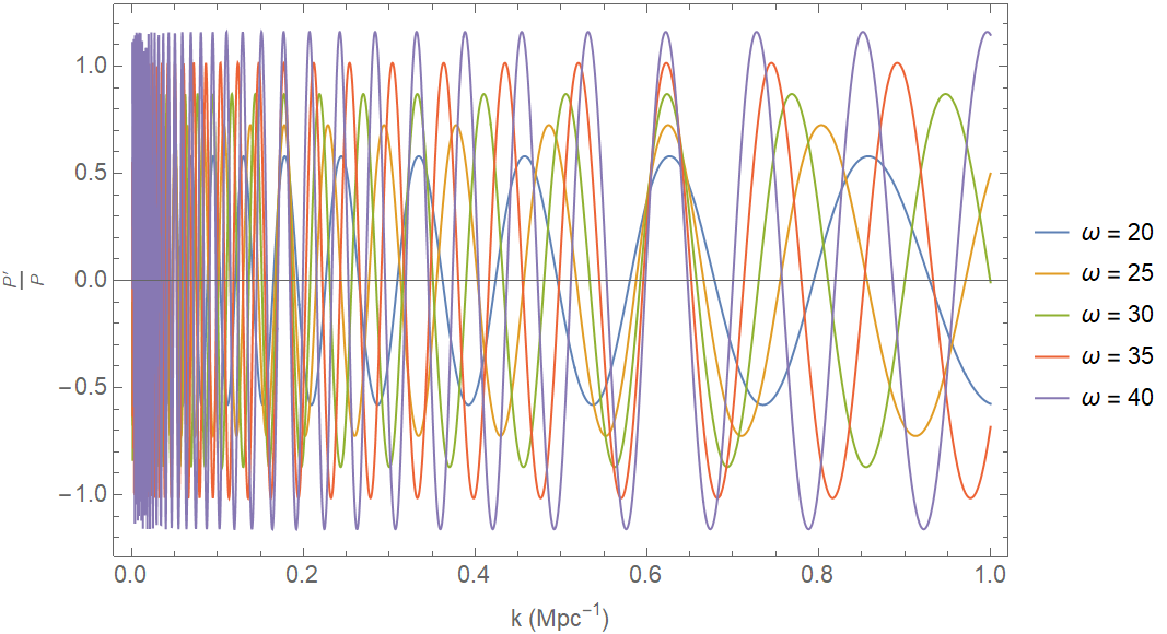
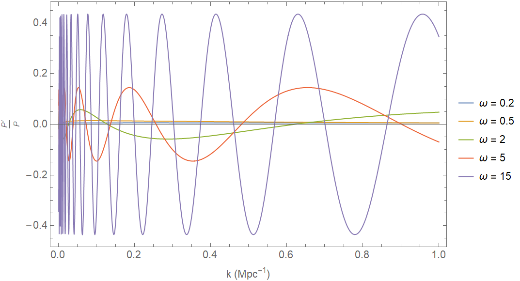
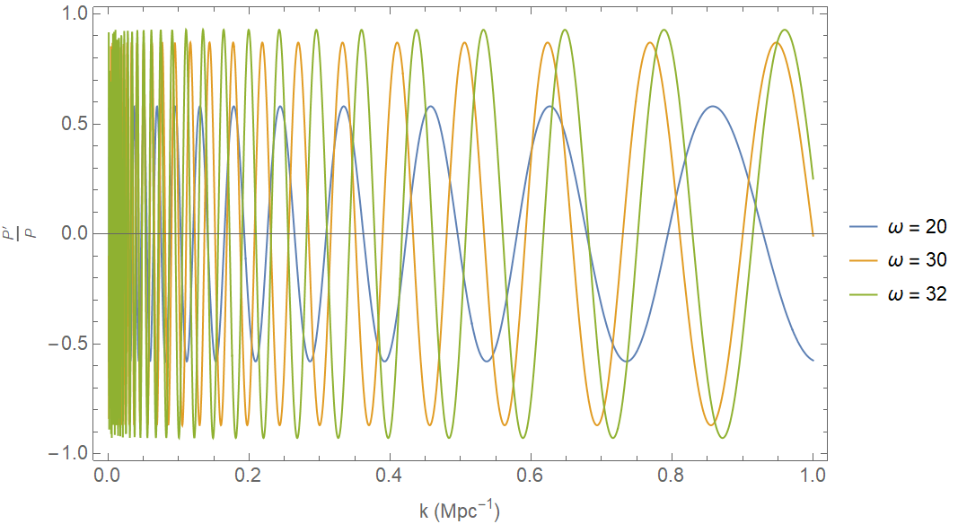
It corresponds physically to the inflaton traversing only a small fraction of one monodromy period during the CMB window, which is exactly what one expects in a broad class of controlled type IIB flux/brane constructions. These models remain Planck-viable with tiny modulation amplitudes and are fully embedded in the same string framework that produces the more commonly discussed high-frequency cases McAllister:2008hb ; Flauger:2009ab . Future experiments (CMB-S4, LiteBIRD) will be sensitive to this low-$\omega$ tail. To have a full understanding on the values of $\omega$ that are allowed, let us plot $\frac{P^{\prime}}{P}$ as a function of the wavenumber for various frequencies in the range $\omega=[0,40]$. Note that we take $P(k)=P_{0}(k)\left(1+A\cos\left(\omega\ln k+\phi-\omega\ln k_{*}\right)\right)$, with $k_{*}=0.05$Mpc^-1, $A=0.029$ and $\frac{\phi}{2\pi}=0.698$ which are the optimal values for $A$ and $\phi$ from CMB studies Zeng:2018ufm . As it can be seen in Fig. 1, the optimal frequency range that guarantees $\frac{P^{\prime}}{P}\ll 1$ is $\omega=[0,30]$, so we confine ourselves to this range of frequencies in what follows. Let us proceed to the possible observable effects in the context of our work, so by using the master equation (48) and the definition of the spectral index,

$$n_{s}^{X}=1+\frac{d\ln P_{X}(k)}{d\ln k}\,,$$

(92)

the true spectral index is essentially,

$$n_{s}^{eff}=1+\frac{d\ln P_{eff}(k)}{d\ln k}\,,$$

(93)

so in view of Eq. (48), the spectral index becomes,

$$n_{s}^{eff}=1+\frac{d\ln P(k)}{d\ln k}+\frac{\sigma_{\ln k}^{2}}{2}\frac{d^{3}\ln P(k)}{d(\ln k)^{3}}\,.$$

(94)

One major prediction of this work, which is absent in the pure oscillatory spectrum without smoothing, is that there might be measurable differences in the spectral index of the TT and EE modes, that is, in the quantity $n_{s}^{TT}-n_{s}^{EE}$. Let us calculate this in detail. We first consider the case that $\omega$ is allowed to take values in the range $\omega=[1,30]$, so $\omega>1$. For the TT and EE power spectrum for $\omega=[1,30]$ we have,

		$\displaystyle n_{s}^{TT}-1=n_{s}^{PL}-1-A\omega\sin(\omega\ln k-\omega\ln k_{TT}+\phi_{TT})$		(95)
		$\displaystyle+\frac{\sigma_{TT}^{2}}{2}\Big[-\frac{2A^{3}\omega^{3}\sin^{3}(\omega\ln k-\omega\ln k_{TT}+\phi_{TT})}{(A\cos(\omega\ln k-\omega\ln k_{TT}+\phi_{TT})+1)^{3}}-\frac{3A^{2}\omega^{3}\sin(\omega\ln k-\omega\ln k_{TT}+\phi_{TT})\cos(\omega\ln k-\omega\ln k_{TT}+\phi_{TT})}{(A\cos(\omega\ln k-\omega\ln k_{TT}+\phi_{TT})+1)^{2}}$
		$\displaystyle+\frac{A\omega^{3}\sin(\omega\ln k-\omega\ln k_{TT}+\phi_{TT})}{A\cos(\omega\ln k-\omega\ln k_{TT}+\phi_{TT})+1}\Big]\,,$

		$\displaystyle n_{s}^{EE}-1=n_{s}^{PL}-1-A\omega\sin(\omega\ln k-\omega\ln k_{EE}+\phi_{EE})$		(96)
		$\displaystyle+\frac{\sigma_{EE}^{2}}{2}\Big[-\frac{2A^{3}\omega^{3}\sin^{3}(\omega\ln k-\omega\ln k_{EE}+\phi_{EE})}{(A\cos(\omega\ln k-\omega\ln k_{EE}+\phi_{EE})+1)^{3}}-\frac{3A^{2}\omega^{3}\sin(\omega\ln k-\omega\ln k_{EE}+\phi_{EE})\cos(\omega\ln k-\omega\ln k_{EE}+\phi_{EE})}{(A\cos(\omega\ln k-\omega\ln k_{EE}+\phi_{EE})+1)^{2}}$
		$\displaystyle+\frac{A\omega^{3}\sin(\omega\ln k-\omega\ln k_{EE}+\phi_{EE})}{A\cos(\omega\ln k-\omega\ln k_{EE}+\phi_{EE})+1}\Big]\,,$

for the spectral indices of the TT and EE spectrums, thus, the difference $n_{s}^{TT}-n_{s}^{EE}$ becomes,

		$\displaystyle n_{s}^{TT}-n_{s}^{EE}=\frac{\sigma_{TT}^{2}}{2}\Big[-\frac{2A^{3}\omega^{3}\sin^{3}(\omega\ln k-\omega\ln k_{TT}+\phi_{TT})}{(A\cos(\omega\ln k-\omega\ln k_{TT}+\phi_{TT})+1)^{3}}$		(97)
		$\displaystyle-\frac{3A^{2}\omega^{3}\sin(\omega\ln k-\omega\ln k_{TT}+\phi_{TT})\cos(\omega\ln k-\omega\ln k_{TT}+\phi_{TT})}{(A\cos(\omega\ln k-\omega\ln k_{TT}+\phi_{TT})+1)^{2}}$
		$\displaystyle+\frac{A\omega^{3}\sin(\omega\ln k-\omega\ln k_{TT}+\phi_{TT})}{A\cos(\omega\ln k-\omega\ln k_{TT}+\phi_{TT})+1}\Big]$
		$\displaystyle-\frac{\sigma_{EE}^{2}}{2}\Big[-\frac{2A^{3}\omega^{3}\sin^{3}(\omega\ln k-\omega\ln k_{EE}+\phi_{EE})}{(A\cos(\omega\ln k-\omega\ln k_{EE}+\phi_{EE})+1)^{3}}-\frac{3A^{2}\omega^{3}\sin(\omega\ln k-\omega\ln k_{EE}+\phi_{EE})\cos(\omega\ln k-\omega\ln k_{EE}+\phi_{EE})}{(A\cos(\omega\ln k-\omega\ln k_{EE}+\phi_{EE})+1)^{2}}$
		$\displaystyle+\frac{A\omega^{3}\sin(\omega\ln k-\omega\ln k_{EE}+\phi_{EE})}{A\cos(\omega\ln k-\omega\ln k_{EE}+\phi_{EE})+1}\Big]-A\omega\sin(\omega\ln k-\omega\ln k_{TT}+\phi_{TT})+A\omega\sin(\omega\ln k-\omega\ln k_{EE}+\phi_{EE})\,,$

where $n_{s}^{PL}$ is the spectral index corresponding to $P_{0}(k)$ which is the power-law part of the primordial power spectrum. This difference between the TT and EE inferred spectral indices $n_{s}^{TT}-n_{s}^{EE}$ is absent in pure power-law power spectrum. Such an effect is below the sensitivity of current experiments, but may become detectable with upcoming high-resolution measurements, such as those from the Simons Observatory or future CMB Stage-4 experiments. However, such analysis must be performed with full statistical methods, a task which extends the purposes of this introductory work. Now we can also obtain a small frequency limit of the quantity $n_{s}^{TT}-n_{s}^{EE}$, so for small frequencies we have for the EE and TT spectral indices,

$$n_{s}^{TT}-1=n_{s}^{PL}-1-A\omega\left(1-\frac{1}{2}\omega^{2}\sigma_{TT}^{2}\right)\sin(\omega\ln k+\phi_{TT}-\omega\ln k_{TT})\,,$$

(98)

$$n_{s}^{EE}-1=n_{s}^{PL}-1-A\omega\left(1-\frac{1}{2}\omega^{2}\sigma_{EE}^{2}\right)\sin(\omega\ln k+\phi_{EE}-\omega\ln k_{EE})\,,$$

(99)

From the above two equations (98) and (99), the difference $n_{s}^{TT}-n_{s}^{EE}$ is,

$$n_{s}^{TT}-n_{s}^{EE}=-A\omega\left(1-\frac{1}{2}\omega^{2}\sigma_{TT}^{2}\right)\sin(\omega\ln k+\phi_{TT}-\omega\ln k_{TT})+A\omega\left(1-\frac{1}{2}\omega^{2}\sigma_{EE}^{2}\right)\sin(\omega\ln k+\phi_{EE}-\omega\ln k_{EE})\,.$$

(100)

The effect of the smoothing on the running of the spectral index $a_{s}=\frac{dn_{s}}{d\ln k}$ must also be taken into account, and by taking into account the effects of the smoothing, the running of the spectral index acquires an extra correction term,

		$\displaystyle\Big(\frac{dn_{s}}{d\ln k}\Big)^{smoothed}=\frac{1}{2}\sigma_{\ln k}^{2}\Big(-\frac{3A^{2}\omega^{4}\cos^{2}(\omega\ln k-\omega\ln k_{*}+\phi_{k})}{(A\cos(\omega\ln k-\omega\ln k_{*}+\phi_{k})+1)^{2}}+\frac{4A^{2}\omega^{4}\sin^{2}(\omega\ln k-\omega\ln k_{*}+\phi_{k})}{(A\cos(\omega\ln k-\omega\ln k_{*}+\phi_{k})+1)^{2}}$		(101)
		$\displaystyle-\frac{12A^{3}\omega^{4}\sin^{2}(\omega\ln k-\omega\ln k_{*}+\phi_{k})\cos(\omega\ln k-\omega\ln k_{*}+\phi_{k})}{(A\cos(\omega\ln k-\omega\ln k_{*}+\phi_{k})+1)^{3}}-\frac{6A^{4}\omega^{4}\sin^{4}(\omega\ln k-\omega\ln k_{*}+\phi_{k})}{(A\cos(\omega\ln k-\omega\ln k_{*}+\phi_{k})+1)^{4}}$
		$\displaystyle+\frac{A\omega^{4}\cos(\omega\ln k-\omega\ln k_{*}+\phi_{k})}{A\cos(\omega\ln k-\omega\ln k_{*}+\phi_{k})+1}\Big)\,.$

A comparison between the TT- and EE-derived constraints on the spectral index $n_{s}$ may provide a useful consistency test. Specifically, independent TT-only and EE-only fits may infer slightly different effective values of the spectral index $n_{s}$, because smoothing-induced distortions will project differently through the temperature and the polarization transfer functions. The detailed statistical significance of such effects requires a dedicated analysis, which lies beyond the scope of this introductory article. We mainly aimed to quantify the effects of a probabilistic smoothing on the power spectrum caused by an extended recombination era. A minimal Fisher matrix analysis is attempted though in the next section, for the general observable effects of the smoothing scale.

References

- (1) A. D. Linde, Lect. Notes Phys. 738 (2008) 1 [arXiv:0705.0164 [hep-th]].
- (2) D. S. Gorbunov and V. A. Rubakov, “Introduction to the theory of the early universe: Cosmological perturbations and inflationary theory,” Hackensack, USA: World Scientific (2011) 489 p;
- (3) A. Linde, arXiv:1402.0526 [hep-th];
- (4) D. H. Lyth and A. Riotto, Phys. Rept. 314 (1999) 1 [hep-ph/9807278].
- (5) M. H. Abitbol et al. [Simons Observatory], Bull. Am. Astron. Soc. 51 (2019), 147 [arXiv:1907.08284 [astro-ph.IM]].
- (6) E. Allys et al. [LiteBIRD], PTEP 2023 (2023) no.4, 042F01 doi:10.1093/ptep/ptac150 [arXiv:2202.02773 [astro-ph.IM]].
- (7) S. Hild, M. Abernathy, F. Acernese, P. Amaro-Seoane, N. Andersson, K. Arun, F. Barone, B. Barr, M. Barsuglia and M. Beker, et al. Class. Quant. Grav. 28 (2011), 094013 doi:10.1088/0264-9381/28/9/094013 [arXiv:1012.0908 [gr-qc]].
- (8) J. Baker, J. Bellovary, P. L. Bender, E. Berti, R. Caldwell, J. Camp, J. W. Conklin, N. Cornish, C. Cutler and R. DeRosa, et al. [arXiv:1907.06482 [astro-ph.IM]].
- (9) T. L. Smith and R. Caldwell, Phys. Rev. D 100 (2019) no.10, 104055 doi:10.1103/PhysRevD.100.104055 [arXiv:1908.00546 [astro-ph.CO]].
- (10) J. Crowder and N. J. Cornish, Phys. Rev. D 72 (2005), 083005 doi:10.1103/PhysRevD.72.083005 [arXiv:gr-qc/0506015 [gr-qc]].
- (11) T. L. Smith and R. Caldwell, Phys. Rev. D 95 (2017) no.4, 044036 doi:10.1103/PhysRevD.95.044036 [arXiv:1609.05901 [gr-qc]].
- (12) N. Seto, S. Kawamura and T. Nakamura, Phys. Rev. Lett. 87 (2001), 221103 doi:10.1103/PhysRevLett.87.221103 [arXiv:astro-ph/0108011 [astro-ph]].
- (13) S. Kawamura, M. Ando, N. Seto, S. Sato, M. Musha, I. Kawano, J. Yokoyama, T. Tanaka, K. Ioka and T. Akutsu, et al. [arXiv:2006.13545 [gr-qc]].
- (14) A. Weltman, P. Bull, S. Camera, K. Kelley, H. Padmanabhan, J. Pritchard, A. Raccanelli, S. Riemer-Sørensen, L. Shao and S. Andrianomena, et al. Publ. Astron. Soc. Austral. 37 (2020), e002 doi:10.1017/pasa.2019.42 [arXiv:1810.02680 [astro-ph.CO]].
- (15) P. Auclair et al. [LISA Cosmology Working Group], [arXiv:2204.05434 [astro-ph.CO]].
- (16) G. Agazie et al. [NANOGrav], Astrophys. J. Lett. 951 (2023) no.1, L8 doi:10.3847/2041-8213/acdac6 [arXiv:2306.16213 [astro-ph.HE]].
- (17) S. Vagnozzi, JHEAp 39 (2023), 81-98 doi:10.1016/j.jheap.2023.07.001 [arXiv:2306.16912 [astro-ph.CO]].
- (18) V. K. Oikonomou, Phys. Rev. D 108 (2023) no.4, 043516 doi:10.1103/PhysRevD.108.043516 [arXiv:2306.17351 [astro-ph.CO]].
- (19) C. Zeng, E. D. Kovetz, X. Chen, Y. Gong, J. B. Muñoz and M. Kamionkowski, Phys. Rev. D 99 (2019) no.4, 043517 doi:10.1103/PhysRevD.99.043517 [arXiv:1812.05105 [astro-ph.CO]].
- (20) G. Domènech and M. Kamionkowski, JCAP 11 (2019), 040 doi:10.1088/1475-7516/2019/11/040 [arXiv:1905.04323 [astro-ph.CO]].
- (21) U. H. Danielsson, Phys. Rev. D 66 (2002), 023511 doi:10.1103/PhysRevD.66.023511 [arXiv:hep-th/0203198 [hep-th]].
- (22) M. G. Jackson and G. Shiu, Phys. Rev. D 88 (2013) no.12, 123511 doi:10.1103/PhysRevD.88.123511 [arXiv:1303.4973 [hep-th]].
- (23) A. Kempf, Phys. Rev. D 63 (2001), 083514 doi:10.1103/PhysRevD.63.083514 [arXiv:astro-ph/0009209 [astro-ph]].
- (24) R. Easther, B. R. Greene, W. H. Kinney and G. Shiu, Phys. Rev. D 67 (2003), 063508 doi:10.1103/PhysRevD.67.063508 [arXiv:hep-th/0110226 [hep-th]].
- (25) J. Martin and R. Brandenberger, Phys. Rev. D 68 (2003), 063513 doi:10.1103/PhysRevD.68.063513 [arXiv:hep-th/0305161 [hep-th]].
- (26) X. Chen, R. Easther and E. A. Lim, JCAP 04 (2008), 010 doi:10.1088/1475-7516/2008/04/010 [arXiv:0801.3295 [astro-ph]].
- (27) R. Flauger, L. McAllister, E. Pajer, A. Westphal and G. Xu, JCAP 06 (2010), 009 doi:10.1088/1475-7516/2010/06/009 [arXiv:0907.2916 [hep-th]].
- (28) L. Covi, J. Hamann, A. Melchiorri, A. Slosar and I. Sorbera, Phys. Rev. D 74 (2006), 083509 doi:10.1103/PhysRevD.74.083509 [arXiv:astro-ph/0606452 [astro-ph]].
- (29) J. Hamann, L. Covi, A. Melchiorri and A. Slosar, Phys. Rev. D 76 (2007), 023503 doi:10.1103/PhysRevD.76.023503 [arXiv:astro-ph/0701380 [astro-ph]].
- (30) D. K. Hazra, M. Aich, R. K. Jain, L. Sriramkumar and T. Souradeep, JCAP 10 (2010), 008 doi:10.1088/1475-7516/2010/10/008 [arXiv:1005.2175 [astro-ph.CO]].
- (31) A. Shafieloo and T. Souradeep, Phys. Rev. D 70 (2004), 043523 doi:10.1103/PhysRevD.70.043523 [arXiv:astro-ph/0312174 [astro-ph]].
- (32) A. Achúcarro, V. Atal, P. Ortiz and J. Torrado, Phys. Rev. D 89 (2014) no.10, 103006 doi:10.1103/PhysRevD.89.103006 [arXiv:1311.2552 [astro-ph.CO]].
- (33) D. K. Hazra, A. Shafieloo and T. Souradeep, JCAP 11 (2014), 011 doi:10.1088/1475-7516/2014/11/011 [arXiv:1406.4827 [astro-ph.CO]].
- (34) X. Chen, M. H. Namjoo and Y. Wang, JCAP 02 (2015), 027 doi:10.1088/1475-7516/2015/02/027 [arXiv:1411.2349 [astro-ph.CO]].
- (35) G. Nicholson and C. R. Contaldi, JCAP 07 (2009), 011 doi:10.1088/1475-7516/2009/07/011 [arXiv:0903.1106 [astro-ph.CO]].
- (36) P. Hunt and S. Sarkar, JCAP 12 (2015), 052 doi:10.1088/1475-7516/2015/12/052 [arXiv:1510.03338 [astro-ph.CO]].
- (37) M. Braglia, X. Chen and D. K. Hazra, JCAP 06 (2021), 005 doi:10.1088/1475-7516/2021/06/005 [arXiv:2103.03025 [astro-ph.CO]].
- (38) M. Braglia, X. Chen and D. K. Hazra, Eur. Phys. J. C 82 (2022) no.5, 498 doi:10.1140/epjc/s10052-022-10461-3 [arXiv:2106.07546 [astro-ph.CO]].
- (39) A. Antony and S. Jain, Eur. Phys. J. C 82 (2022) no.8, 687 doi:10.1140/epjc/s10052-022-10616-2 [arXiv:2110.06837 [astro-ph.CO]].
- (40) D. K. Hazra, A. Antony and A. Shafieloo, JCAP 08 (2022) no.08, 063 doi:10.1088/1475-7516/2022/08/063 [arXiv:2201.12000 [astro-ph.CO]].
- (41) A. Antony, F. Finelli, D. K. Hazra and A. Shafieloo, Phys. Rev. Lett. 130 (2023) no.11, 111001 doi:10.1103/PhysRevLett.130.111001 [arXiv:2202.14028 [astro-ph.CO]].
- (42) E. Silverstein and A. Westphal, Phys. Rev. D 78 (2008), 106003 doi:10.1103/PhysRevD.78.106003 [arXiv:0803.3085 [hep-th]].
- (43) L. McAllister, E. Silverstein and A. Westphal, Phys. Rev. D 82 (2010), 046003 doi:10.1103/PhysRevD.82.046003 [arXiv:0808.0706 [hep-th]].
- (44) S. R. Behbahani, A. Dymarsky, M. Mirbabayi and L. Senatore, JCAP 12 (2012), 036 doi:10.1088/1475-7516/2012/12/036 [arXiv:1111.3373 [hep-th]].
- (45) X. Wang, B. Feng, M. Li, X. L. Chen and X. Zhang, Int. J. Mod. Phys. D 14 (2005), 1347 doi:10.1142/S0218271805006985 [arXiv:astro-ph/0209242 [astro-ph]].
- (46) R. Easther, B. R. Greene, W. H. Kinney and G. Shiu, Phys. Rev. D 66 (2002), 023518 doi:10.1103/PhysRevD.66.023518 [arXiv:hep-th/0204129 [hep-th]].
- (47) V. Bozza, M. Giovannini and G. Veneziano, JCAP 05 (2003), 001 doi:10.1088/1475-7516/2003/05/001 [arXiv:hep-th/0302184 [hep-th]].
- (48) C. Dvorkin and W. Hu, Phys. Rev. D 82 (2010), 043513 doi:10.1103/PhysRevD.82.043513 [arXiv:1007.0215 [astro-ph.CO]].
- (49) C. Dvorkin and W. Hu, Phys. Rev. D 81 (2010), 023518 doi:10.1103/PhysRevD.81.023518 [arXiv:0910.2237 [astro-ph.CO]].
- (50) M. J. Mortonson, H. V. Peiris and R. Easther, Phys. Rev. D 83 (2011), 043505 doi:10.1103/PhysRevD.83.043505 [arXiv:1007.4205 [astro-ph.CO]].
- (51) P. Adshead, W. Hu, C. Dvorkin and H. V. Peiris, Phys. Rev. D 84 (2011), 043519 doi:10.1103/PhysRevD.84.043519 [arXiv:1102.3435 [astro-ph.CO]].
- (52) J. A. Adams, B. Cresswell and R. Easther, Phys. Rev. D 64 (2001), 123514 doi:10.1103/PhysRevD.64.123514 [arXiv:astro-ph/0102236 [astro-ph]].
- (53) W. Hu, Phys. Rev. D 65 (2002), 023003 doi:10.1103/PhysRevD.65.023003 [arXiv:astro-ph/0108090 [astro-ph]].
- (54) Y. Akrami et al. [Planck], Astron. Astrophys. 641 (2020), A10 doi:10.1051/0004-6361/201833887 [arXiv:1807.06211 [astro-ph.CO]].