跳到论文正文
W Papers独立论文阅读器 arXiv:2605.19170 论文正文 计算阅读时间 · 0%
引用这篇论文根据当前论文元数据生成,正式投稿前建议核对。


License: CC BY 4.0
arXiv:2605.19170v2 [stat.ML] 23 May 2026

Reducing Diffusion Model Memorization with Higher Order Langevin Dynamics

Benjamin Sterling
Department of Applied Math & Statistics
Stony Brook University
Stony Brook, NY 11790
benjamin.sterling@stonybrook.edu
Mónica F. Bugallo
Department of Electrical and Computer Engineering
Stony Brook University
Stony Brook, NY 11790
monica.bugallo@stonybrook.edu
Tom Tirer
Faculty of Engineering
Bar-Ilan University
Ramat-Gan 5290002, Israel
tirer.tom@biu.ac.il
Abstract

Diffusion/score-based models have emerged as powerful generative models, capable of generating high-quality samples that mimic the training data distribution. However, it has been observed that they are prone to reproducing training samples—known as “memorization”—potentially violating copyright and privacy. In this paper, we study the effect of Higher-Order Langevin Dynamics (HOLD) on this phenomenon. HOLD diffusion processes introduce auxiliary variables; if the data variable is interpreted as “position,” then the auxiliary variables can be interpreted as “velocity” and “acceleration,” depending on the chosen order of the model. They were originally proposed based on the intuition that they regularize the trajectories of the data variable by implicitly imposing additional dynamical constraints. Our work provides, to our knowledge, the first theoretical characterization of the regularization effect of HOLD. Specifically, we show that in HOLD, the dynamics of the data variable are governed by a low-pass-filtered version of the learned score function, with smoothness increasing with the order of HOLD. We then analyze the optimal empirical score and the possibility of distribution collapse. Together, our results explain the mitigation of memorization as the model order increases. Finally, we present an empirical study on real-world data that supports our theory and highlights this distinct advantage of HOLD over standard diffusion in practice.

1 Introduction

First introduced in (Sohl-Dickstein et al., 2015) and later refined in (Song and Ermon, 2019; Ho et al., 2020; Song et al., 2021), Denoising Diffusion Models (DDMs) have demonstrated remarkable success in generating high quality samples from intractable, high-dimensional data distributions. They are based on generating samples from a tractable latent distribution (typically, standard normal) and converting them to samples from the target distribution via iterative denoising with gradually decreasing noise level. Trained DDMs have also emerged as powerful generative priors for editing and restoring signals and images (Meng et al., 2022; Kawar et al., 2022; Abu-Hussein et al., 2022; Garber and Tirer, 2024, 2025). Recently, however, it has been observed that DDMs are prone to exactly reproducing training samples (Carlini et al., 2023; Somepalli et al., 2023). This phenomenon, termed “memorization”, can have severe negative implications, such as violating copyright and privacy.

Memorization of DDMs has recently become a topic of interest both experimentally and theoretically. (Yoon et al., 2023) suggested that diffusion models either “generalize” or “memorize” in a mutually exclusive manner, and that overfitting in this context is not “benign” (unlike certain phenomena in linear regression (Bartlett et al., 2020)). In fact, a key factor for diffusion memorization is that, if one considers an unconstrained denoiser/score function, the optimum of the empirical mean squared error loss used in training has an analytical form (Karras et al., 2022), which necessarily outputs a sample from the training set as the noise level decreases (Yi et al., 2023; Zhang et al., 2024) (more details in Section 2). The work of (Kadkhodaie et al., 2024) argues that diffusion models generalize because of inductive biases; their network architecture encourages shrinkage towards geometry-adaptive harmonic bases that are informed by the data distribution. (Zhang et al., 2024) performs similar experiments, demonstrating a separation between memorization and generalization regimes depending on the dataset size. They argue that in the generalization regime, the learned distributions are largely independent of model architectures and are instead most heavily influenced by the training data. (Gu et al., 2025) empirically studies the relationship between dataset size, the memorization ratio, and different state-of-the-art architectures. Other works on diffusion memorization (Bonnaire et al., 2025; George et al., 2026) include theoretical analyses based on the random features model. In particular, (Bonnaire et al., 2025) empirically and theoretically studies the level of memorization along the optimization. Their results suggest that one can avoid or mitigate memorization using early stopping within a range of time that depends on the dataset size. However, in practice, especially in the presence of a biased validation dataset, it is hard to gauge when to stop. This study motivates the question of whether there are other ways to reduce memorization besides early stopping.

In parallel to the works analyzing memorization in diffusion models, there have been separate methods developed with the goals of shortening and smoothing the diffusion model’s path from target and latent distributions through the introduction of higher-order auxiliary variables. Intuitively, if the data variable is interpreted as “position,” then the auxiliary variables can be interpreted as “velocity” and “acceleration,” depending on the chosen order of the model. (Dockhorn et al., 2022) proposed critically-damped Langevin dynamics (CLD), which introduces a velocity variable, and studies the effect of critical damping on the diffusion dynamics. In this context, critical-damping refers to choosing parameters so that the diffusion forward process’s matrix has a single geometric eigenvalue and thus increases the speed of convergence along diffusion time. Inspired by this work, higher-order Langevin dynamics (HOLD) (Shi and Liu, 2024) was introduced to simplify the diffusion process of CLD as an Ornstein–Uhlenbeck process superimposed with a skew symmetric variable coupling. Follow ups of this work have showed that it is possible to critically damp HOLD (Sterling and Bugallo, 2025; Sterling et al., 2025b), and that using HOLD helps to defend DDMs against membership inference attacks (Sterling et al., 2025a).

In this paper, we study the effect of higher-order diffusion modeling on memorization. First, we close a gap in the literature regarding the regularization effect of these models. These models were originally proposed based on the intuition that they regularize the trajectories of the data variable by implicitly imposing additional dynamical constraints; this regularization effect lacks theoretical justification. We provide, to our knowledge, the first rigorous characterization of the regularization effect of HOLD. Specifically, we utilize the Laplace transform to demonstrate the low-pass filtering effect of the model order on the learned score function. Then, we analyze the optimal empirical score function of HOLD models and present a result on the impossibility of distribution collapse. Altogether, these findings explain the mitigation of memorization as the model order increases. Finally, we present an empirical study on real-world data that supports our theory. Namely, we measure the generation quality and memorization rate of models of different orders along training for two different datasets: the CelebA dataset (extending the setup of (Bonnaire et al., 2025)) and the CIFAR-10 dataset. The experiments show that HOLD models offer similar Fréchet Inception Distance (FID) results as plain (first-order) diffusion models, while memorization, measured as in previous works, is delayed and attenuated as the model order increases, aligned with our theory.

2 Background

2.1 Score-based generative modeling and memorization by the optimal empirical score

Previous works (Karras et al., 2022; Yi et al., 2023) have derived that the regular score matching, which uses an empirical training objective, has a closed form optimal score function that is based on a weighted average of the training data and even converges to being dependent solely on the single training sample closest to its input as t→0t\to 0.

Let us present this formally for the Ornstein–Uhlenbeck process, a standard DDM framework, which possesses the following stochastic differential equation (SDE):

d​𝐱t=−ξ​𝐱t​d​t+2​ξ​L−1​d​𝐰t,d\mathbf{x}_{t}=-\xi\mathbf{x}_{t}dt+\sqrt{2\xi L^{-1}}d\mathbf{w}_{t},

where L−1L^{-1} and ξ\xi are algorithmic parameters and 𝐰t\mathbf{w}_{t} represents the standard Wiener process. In this forward process, given a data sample 𝐱0\mathbf{x}_{0}, a sample 𝐱t\mathbf{x}_{t} can be drawn according to 𝐱t=exp⁡(−ξ​t)​𝐱0+σt​ϵ\mathbf{x}_{t}=\exp(-\xi t)\mathbf{x}_{0}+\sigma_{t}\boldsymbol{\epsilon}, where σt2=L−1​(1−exp⁡(−2​ξ​t))\sigma_{t}^{2}=L^{-1}(1-\exp(-2\xi t)) and ϵ∼𝒩​(𝟎,𝐈)\boldsymbol{\epsilon}\sim\mathcal{N}(\mathbf{0},\mathbf{I}).

The generation of data samples by DDMs is based on the fact that there is an associated backward SDE with the same marginal distribution of 𝐱t\mathbf{x}_{t} (Anderson, 1982; Song et al., 2021):

d​𝐱t\displaystyle d\mathbf{x}_{t} =−ξ​(𝐱t+2​L−1​𝐬​(𝐱t,t))​d​t+2​ξ​L−1​d​𝐰¯t,\displaystyle=-\xi\left(\mathbf{x}_{t}+2L^{-1}\mathbf{s}(\mathbf{x}_{t},t)\right)dt+\sqrt{2\xi L^{-1}}d\bar{\mathbf{w}}_{t}, (1)

where 𝐬​(⋅,t)=∇𝐱log⁡pt​(⋅)\mathbf{s}(\cdot,t)=\nabla_{\mathbf{x}}\log p_{t}(\cdot) is the score function of 𝐱t\mathbf{x}_{t} (with ptp_{t} denoting the distribution of 𝐱t\mathbf{x}_{t}). The score function is modeled by 𝐬θ​(⋅,t)\mathbf{s}_{\theta}(\cdot,t) and learned during training. For the standard training objective

ℒ\displaystyle\mathcal{L} =𝔼t∼𝒰​(0,1),𝐱0,ϵ∼𝒩​(𝟎,𝐈)​‖ϵ+σt​𝐬θ​(𝐱t,t)‖2,\displaystyle=\mathbb{E}_{t\sim\mathcal{U}(0,1),\mathbf{x}_{0},\boldsymbol{\epsilon}\sim\mathcal{N}(\mathbf{0},\mathbf{I})}||\boldsymbol{\epsilon}+\sigma_{t}\mathbf{s}_{\theta}(\mathbf{x}_{t},t)||^{2}, (2)

with the empirical distribution p​(𝐱0)=1ntrain​∑k=1ntrainδ​(𝐱0−𝐱0(k))p(\mathbf{x}_{0})=\frac{1}{n_{\text{train}}}\sum\nolimits_{k=1}^{n_{\text{train}}}\delta(\mathbf{x}_{0}-\mathbf{x}_{0}^{(k)}), the optimal (unconstrained) score function is given by 𝐬emp​(𝐱,t)=∇𝐱log⁡ptemp, OU​(𝐱)\mathbf{s}_{\text{emp}}(\mathbf{x},t)=\nabla_{\mathbf{x}}\log p^{\text{emp, OU}}_{t}(\mathbf{x}), where

ptemp, OU​(𝐱)\displaystyle p^{\text{emp, OU}}_{t}(\mathbf{x}) =1ntrain​∑k=1ntrain(2​π​σt2)−h/2​exp⁡(−12​σt2​‖𝐱−exp⁡(−ξ​t)​𝐱0(k)‖2).\displaystyle=\frac{1}{n_{\text{train}}}\sum_{k=1}^{n_{\text{train}}}(2\pi\sigma_{t}^{2})^{-h/2}\exp\left(-\frac{1}{2\sigma_{t}^{2}}\bigg\|\mathbf{x}-\exp(-\xi t)\mathbf{x}^{(k)}_{0}\bigg\|^{2}\right).

That is,

semp​(𝐱,t)\displaystyle s_{\text{emp}}(\mathbf{x},t) =−1σt2​(𝐱−exp⁡(−ξ​t)​∑k=1ntrain𝒩​(𝐱∣exp⁡(−ξ​t)​𝐱0(k),σt2​𝐈)​𝐱0(k)∑k=1ntrain𝒩​(𝐱∣exp⁡(−ξ​t)​𝐱0(k),σt2​𝐈)).\displaystyle=-\frac{1}{\sigma_{t}^{2}}\left(\mathbf{x}-\exp(-\xi t)\frac{\sum_{k=1}^{n_{\mathrm{train}}}\mathcal{N}(\mathbf{x}\mid\exp(-\xi t)\mathbf{x}^{(k)}_{0},\sigma_{t}^{2}\mathbf{I})\,\,\mathbf{x}^{(k)}_{0}}{\sum_{k=1}^{n_{\mathrm{train}}}\mathcal{N}(\mathbf{x}\mid\exp(-\xi t)\mathbf{x}^{(k)}_{0},\sigma_{t}^{2}\mathbf{I})}\right).

which follows the description above (i.e., weighted average of the training samples that converges to the nearest training sample as t→0t\to 0).

This conveys that diffusion models generalize due to explicit and implicit inductive biases, while approaching the unconstrained empirical optimum, e.g., due to a small number of training samples (Kadkhodaie et al., 2024; Zhang et al., 2024) and/or prolonged training (Bonnaire et al., 2025; George et al., 2026), increases memorization.

2.2 Overview of HOLD

We start this section by providing an overview of HOLD (Shi and Liu, 2024; Sterling et al., 2025b) following the variable conventions used in (Dockhorn et al., 2022). Suppose a data point is expressed as a vector 𝐱0∈ℝh\mathbf{x}_{0}\in\mathbb{R}^{h}. Let α,L−1,{γk}1≤k≤n−1,\alpha,L^{-1},\{\gamma_{k}\}_{1\leq k\leq n-1}, and ξ\xi denote algorithmic parameters, where nn denotes the order of the model. In HOLD, we define the initial diffusion variable 𝐮0=vec⁡(𝐱0,𝐯0(1),𝐯0(2)​…​𝐯0(n−1))\mathbf{u}_{0}=\operatorname{vec}(\mathbf{x}_{0},\mathbf{v}^{(1)}_{0},\mathbf{v}^{(2)}_{0}\ldots\mathbf{v}^{(n-1)}_{0}), where 𝐯0(1),𝐯0(2)​…​𝐯0(n−1)∼iid𝒩​(𝟎,α​L−1​𝐈)\mathbf{v}^{(1)}_{0},\mathbf{v}^{(2)}_{0}\ldots\mathbf{v}^{(n-1)}_{0}\sim_{\text{iid}}\mathcal{N}(\mathbf{0},\alpha L^{-1}\mathbf{I}) are auxiliary variables. Take the following system:

𝐅\displaystyle\mathbf{F} =∑i=1n−1γi​(𝐄i,i+1−𝐄i+1,i)−ξ​𝐄n,n,𝐆=2​ξ​L−1​𝐄n,n,\displaystyle=\sum_{i=1}^{n-1}\gamma_{i}\left(\mathbf{E}_{i,i+1}-\mathbf{E}_{i+1,i}\right)-\xi\mathbf{E}_{n,n},\quad\mathbf{G}=\sqrt{2\xi L^{-1}}\mathbf{E}_{n,n},

where 𝐄i,j∈ℝn×n\mathbf{E}_{i,j}\in\mathbb{R}^{n\times n} is the matrix of all zeros with a one at index pair (i,j)(i,j). The forward process evolves according to the SDE:

d​𝐮t\displaystyle d\mathbf{u}_{t} =ℱ​𝐮t​d​t+𝒢​d​𝐰t,\displaystyle=\mathcal{F}\mathbf{u}_{t}dt+\mathcal{G}d\mathbf{w}_{t}, (3)

where ℱ=𝐅⊗𝐈h\mathcal{F}=\mathbf{F}\otimes\mathbf{I}_{h}, 𝒢=𝐆⊗𝐈h\mathcal{G}=\mathbf{G}\otimes\mathbf{I}_{h} (with ⊗\otimes denoting the Kronecker product), and 𝐰t\mathbf{w}_{t} represents the standard Wiener process. For example, when n=3n=3, the dynamics are governed by:

{d​𝐱t=γ1​𝐯t(1)​d​t,d​𝐯t(1)=(−γ1​𝐱t+γ2​𝐯t(2))​d​t,d​𝐯t(2)=(−γ2​𝐯t(1)−ξ​𝐯t(2))​d​t+2​ξ​L−1​d​𝐰t.\displaystyle\begin{cases}d\mathbf{x}_{t}&=\gamma_{1}\mathbf{v}^{(1)}_{t}dt,\\ d\mathbf{v}^{(1)}_{t}&=\left(-\gamma_{1}\mathbf{x}_{t}+\gamma_{2}\mathbf{v}^{(2)}_{t}\right)dt,\\ d\mathbf{v}^{(2)}_{t}&=\left(-\gamma_{2}\mathbf{v}^{(1)}_{t}-\xi\mathbf{v}^{(2)}_{t}\right)dt+\sqrt{2\xi L^{-1}}d\mathbf{w}_{t}.\end{cases}

Here, the dynamics of 𝐱t\mathbf{x}_{t} are modeled by the “velocity” variable 𝐯t(1)\mathbf{v}^{(1)}_{t} and the “acceleration” variable 𝐯t(2)\mathbf{v}^{(2)}_{t}. In the notation of Equation (3), the 𝐅\mathbf{F} and 𝐆\mathbf{G} matrices for n=3n=3 become:

𝐅\displaystyle\mathbf{F} =(0γ10−γ10γ20−γ2−ξ),𝐆=(000000002​ξ​L−1).\displaystyle=\begin{pmatrix}0&\gamma_{1}&0\\ -\gamma_{1}&0&\gamma_{2}\\ 0&-\gamma_{2}&-\xi\end{pmatrix},\quad\mathbf{G}=\begin{pmatrix}0&0&0\\ 0&0&0\\ 0&0&\sqrt{2\xi L^{-1}}\end{pmatrix}.

It can be shown that 𝐮t\mathbf{u}_{t} that satisfies Equation (3) must be normally distributed (conditioned on 𝐱0\mathbf{x}_{0}), and expressions for the mean and covariance of 𝐮t\mathbf{u}_{t} must satisfy the following differential equations, which can be derived from the Fokker-Planck equations (Särkkä and Solin, 2019),

d​𝝁td​t\displaystyle\frac{d\boldsymbol{\mu}_{t}}{dt} =ℱ​𝝁t,d​𝚺td​t=ℱ​𝚺t+(ℱ​𝚺t)T+𝒢​𝒢T.\displaystyle=\mathcal{F}\boldsymbol{\mu}_{t},\quad\frac{d\boldsymbol{\Sigma}_{t}}{dt}=\mathcal{F}\boldsymbol{\Sigma}_{t}+\left(\mathcal{F}\boldsymbol{\Sigma}_{t}\right)^{T}+\mathcal{G}\mathcal{G}^{T}.

It is proven in (Sterling et al., 2025b) that 𝐮t\mathbf{u}_{t} must also possess the following distribution:

𝐮t\displaystyle\mathbf{u}_{t} ∼𝒩​(𝝁t,𝚺t),𝝁t=exp⁡(ℱ​t)​𝐮0,\displaystyle\sim\mathcal{N}(\boldsymbol{\mu}_{t},\boldsymbol{\Sigma}_{t}),\quad\boldsymbol{\mu}_{t}=\exp(\mathcal{F}t)\mathbf{u}_{0},
𝚺t\displaystyle\boldsymbol{\Sigma}_{t} =L−1𝐈+exp(ℱt)(𝚺0−L−1𝐈)exp(ℱt)T.\displaystyle=L^{-1}\mathbf{I}+\exp(\mathcal{F}t)\left(\boldsymbol{\Sigma}_{0}-L^{-1}\mathbf{I}\right)\exp(\mathcal{F}t)^{T}.

In the forward diffusion process, samples are generated according to 𝐮t=exp⁡(ℱ​t)​𝐮0+𝐋t​ϵfull\mathbf{u}_{t}=\exp(\mathcal{F}t)\mathbf{u}_{0}+\mathbf{L}_{t}\boldsymbol{\epsilon}_{\text{full}}, where ϵ1,ϵ2​…​ϵn∼𝒩​(𝟎,𝐈h),ϵfull=vec⁡(ϵ1,ϵ2​…​ϵn),\boldsymbol{\epsilon}_{1},\boldsymbol{\epsilon}_{2}\ldots\boldsymbol{\epsilon}_{n}\sim\mathcal{N}(\mathbf{0},\mathbf{I}_{h}),\boldsymbol{\epsilon}_{\text{full}}=\operatorname{vec}(\boldsymbol{\epsilon}_{1},\boldsymbol{\epsilon}_{2}\ldots\boldsymbol{\epsilon}_{n}), and 𝐋t=cholesky⁡(𝚺t)\mathbf{L}_{t}=\operatorname{cholesky}(\boldsymbol{\Sigma}_{t}).

The computation of the term exp⁡(ℱ​t)\exp(\mathcal{F}t) is not obvious, and (Shi and Liu, 2024) uses Putzer’s Lemma (Putzer, 1966) to compute it. However, when the parameters of ℱ\mathcal{F} are chosen so that it posses a single geometric eigenvalue s∗=2​n−3s_{*}=\sqrt{2n-3}, as in (Sterling et al., 2025b), then it may be calculated by a finite Taylor Series, understanding that ℱ−s∗​𝐈\mathcal{F}-s_{*}\mathbf{I} is nilpotent:

exp⁡(ℱ​t)=exp⁡(s∗​t)​∑k=0n−1(ℱ−s∗​𝐈)k​tkk!.\displaystyle\exp(\mathcal{F}t)=\exp(s_{*}t)\sum_{k=0}^{n-1}\frac{(\mathcal{F}-s_{*}\mathbf{I})^{k}t^{k}}{k!}. (4)

The loss function under this forward SDE is the same score matching objective that (Dockhorn et al., 2022; Shi and Liu, 2024) use. Instead of modeling the score of the data variable 𝐱t\mathbf{x}_{t} or the score of the full 𝐮t\mathbf{u}_{t}, it suffices to model the score of the last auxiliary variable 𝐯t(n−1)\mathbf{v}^{(n-1)}_{t} by 𝐬θ​(𝐮t,t)\mathbf{s}_{\theta}(\mathbf{u}_{t},t), and learn it with the objective

ℒ\displaystyle\mathcal{L} =𝔼t∼𝒰​(0,1),𝐮0,ϵfull​‖ϵn+𝐬θ​(𝐮t,t)​(𝐋t​[n​h,n​h])‖2.\displaystyle=\mathbb{E}_{t\sim\mathcal{U}(0,1),\mathbf{u}_{0},\boldsymbol{\epsilon}_{\text{full}}}\|\boldsymbol{\epsilon}_{n}+\mathbf{s}_{\theta}(\mathbf{u}_{t},t)\left(\mathbf{L}_{t}[nh,nh]\right)\|^{2}. (5)

The following ordinary differential equation (ODE) (Song et al., 2021) shares the same approximate marginal probability densities as the backwards SDE and may be used for sample generation:

d​𝐮t\displaystyle d\mathbf{u}_{t} =(ℱ​𝐮t−12​𝒢​𝒢T​𝐒θ​(𝐮t,t))​d​t,\displaystyle=\left(\mathcal{F}\mathbf{u}_{t}-\frac{1}{2}\mathcal{G}\mathcal{G}^{T}\mathbf{S}_{\theta}(\mathbf{u}_{t},t)\right)dt, (6)

where 𝐒θ​(𝐮t,t)=vec⁡(𝟎(n−1)​h,𝐬θ​(𝐮t,t))\mathbf{S}_{\theta}(\mathbf{u}_{t},t)=\operatorname{vec}(\mathbf{0}_{(n-1)h},\mathbf{s}_{\theta}(\mathbf{u}_{t},t)). It is further proven in (Sterling et al., 2025b) that the system is critically damped for n≥2n\geq 2, meaning 𝐅\mathbf{F} has a single geometric eigenvalue, if and only if

γn−i\displaystyle\gamma_{n-i} =2​n−3​n2−i24​i2−1,ξ=n​2​n−3,\displaystyle=\sqrt{2n-3}\sqrt{\frac{n^{2}-i^{2}}{4i^{2}-1}},\quad\xi=n\sqrt{2n-3},

assuming a scaling choice of γ1=1\gamma_{1}=1. For further convenience in this paper, define γ¯=∏i=1n−1γi\bar{\gamma}=\prod_{i=1}^{n-1}\gamma_{i}.

3 Theoretical Analysis

This section presents our theoretical analysis of the regularization introduced by the HOLD model and its ability to mitigate memorization.

3.1 In HOLD the score is being low-pass filtered

This subsection argues that HOLD introduces a low-pass filtering effect on the score during the generation procedure. While neither the reverse SDE nor reverse ODE have closed form solutions, we study the reverse ODE given by Equation (6) and analyze the relationship between the score function and generated samples from a signals and systems perspective (Oppenheim et al., 1997).

We start with Lemma 1 below, which assists the proof of our key Theorem 1. Essentially, it is based on taking the Laplace transform of both sides of Equation (6), and identifying recursive patterns.

Lemma 1.

Consider the ODE (6). If the Laplace transform of 𝐱t\mathbf{x}_{t} is 𝐱~​(s)\tilde{\mathbf{x}}(s), the Laplace transform of 𝐬θ​(𝐮t,t)\mathbf{s}_{\theta}(\mathbf{u}_{t},t) is 𝐬~​(s)\tilde{\mathbf{s}}(s) (accounting for tt from both arguments), and P​(s)P(s) is the characteristic polynomial of 𝐅\mathbf{F}, then

𝐱~​(s)\displaystyle\tilde{\mathbf{x}}(s) =−γ¯​ξ​L−1​𝐬~​(s)P​(s)+𝐱~natural​(s),\displaystyle=-\frac{\bar{\gamma}\xi L^{-1}\tilde{\mathbf{s}}(s)}{P(s)}+\tilde{\mathbf{x}}^{\mathrm{natural}}(s),

where 𝐱~natural​(s)\tilde{\mathbf{x}}^{\mathrm{natural}}(s) arises from nonzero 𝐮0\mathbf{u}_{0} and is independent of the score. Its full expression is available in the appendix.

See Appendix A.2 for the proof. Now that we have this result, we may proceed to the following theorem.

Theorem 1.

Let ht(n)=−γ¯​n​2​n−3​L−1​tn−1​exp⁡(−t​2​n−3)h_{t}^{(n)}=-\bar{\gamma}n\sqrt{2n-3}L^{-1}t^{n-1}\exp(-t\sqrt{2n-3}) for n≥2n\geq 2. For model order n≥2n\geq 2, the solution to (6) for the data variable 𝐱t\mathbf{x}_{t} is:

𝐱t=ht(n)∗𝐬θ​(𝐮t,t)+𝐱tnatural,\mathbf{x}_{t}=h_{t}^{(n)}*\mathbf{s}_{\theta}(\mathbf{u}_{t},t)+\mathbf{x}^{\mathrm{natural}}_{t},

where ‘∗*’ denotes the convolution operation (in the time domain).

See Appendix A.3 for the proof. The proof uses the Residue Theorem applied to the equation in Lemma 1. The variables 𝐱~natural​(s)\tilde{\mathbf{x}}^{\mathrm{natural}}(s) and 𝐱tnatural\mathbf{x}^{\mathrm{natural}}_{t} are referred to as “natural” parameters because they both come from nonzero 𝐮0\mathbf{u}_{0}, as opposed to the “forcing” term, −12​𝒢​𝒢T​𝐒θ​(𝐮t,t)-\frac{1}{2}\mathcal{G}\mathcal{G}^{T}\mathbf{S}_{\theta}(\mathbf{u}_{t},t) in Equation (6). It is also noteworthy that the score, 𝐬θ​(𝐮t,t)\mathbf{s}_{\theta}(\mathbf{u}_{t},t) affects 𝐱t\mathbf{x}_{t} only through convolution with ht(n)h_{t}^{(n)}.

Theorem 1 is a novel result that is most useful for theoretical analysis and may also benefit the design of the forward process itself. It does not directly lead to an algorithm to solve for 𝐱t\mathbf{x}_{t} because 𝐬θ\mathbf{s}_{\theta} is a function of 𝐮t\mathbf{u}_{t}, which is itself a function of 𝐱t\mathbf{x}_{t}, as well as the fact that 𝐱tnatural\mathbf{x}^{\mathrm{natural}}_{t} depends on 𝐱0\mathbf{x}_{0} (which is unknown during the backward process).

Both results speak to the optimality of choosing critically damped parameters. It was proven in (Sterling et al., 2025b) that the critically damped parameters are optimal for the following design objective involving the forward matrix 𝐅\mathbf{F}:

minγ2,γ3​…​γn−1,ξ⁡max⁡(Re⁡(eig⁡(𝐅))).\displaystyle\min_{\gamma_{2},\gamma_{3}\ldots\gamma_{n-1},\xi}\max\left(\operatorname{Re}\left(\operatorname{eig}(\mathbf{F})\right)\right). (7)

With Lemma 1 and Theorem 1, one may understand that not choosing critically damped parameters would result in the characteristic polynomial P​(s)=∏i=1n(s−si)P(s)=\prod_{i=1}^{n}(s-s_{i}), which leads to ht(n)=∑i=1nci​exp⁡(si​t)h_{t}^{(n)}=\sum_{i=1}^{n}c_{i}\exp(s_{i}t) (the cic_{i} are the coefficients obtained from the residue theorem). Because the critically damped parameters minimize (7), not using the critically damped parameter choices necessitates the existence of at least one eigenvalue of 𝐅\mathbf{F}, sks_{k} such that sk>s∗s_{k}>s_{*}. The consequence of such a mode ck​exp⁡(sk​t)c_{k}\exp(s_{k}t) is slower convergence along diffusion time, or from a frequency perspective: a mode that allows more high frequencies from 𝐬θ\mathbf{s}_{\theta} pass into 𝐱t\mathbf{x}_{t}. The critically damped parameters therefore represent the filter with the sharpest frequency cutoff.

A simple derivation in Appendix A.5 yields that the solution of the backward ODE associated with the (first-order) Ornstein–Uhlenbeck process: d​𝐱t=−ξ​𝐱t​d​t+2​ξ​L−1​d​𝐰td\mathbf{x}_{t}=-\xi\mathbf{x}_{t}dt+\sqrt{2\xi L^{-1}}d\mathbf{w}_{t} may be expressed with htOU=−ξ​L−1​exp⁡(−ξ​t)h_{t}^{\text{OU}}=-\xi L^{-1}\exp(-\xi t):

𝐱t=exp⁡(−ξ​t)​𝐱0−ξ​L−1​∫0texp⁡(−ξ​(t−τ))​𝐬θ​(𝐱τ,τ)​𝑑τ=exp⁡(−ξ​t)​𝐱0+htOU∗𝐬θ​(𝐱t,t).\mathbf{x}_{t}=\exp(-\xi t)\mathbf{x}_{0}-\xi L^{-1}\int_{0}^{t}\exp(-\xi(t-\tau))\mathbf{s}_{\theta}(\mathbf{x}_{\tau},\tau)d\tau=\exp(-\xi t)\mathbf{x}_{0}+h_{t}^{\text{OU}}*\mathbf{s}_{\theta}(\mathbf{x}_{t},t).

Contrasting this result with Theorem 1 sheds a new light on the inherent regularization of HOLD. It formally shows the smoothing effect of HOLD on the generated sample trajectories, where the “smoothing” is manifested by ht(n)h_{t}^{(n)} acting on the score function as a low-pass filter with stronger attenuation of high frequencies than htOUh_{t}^{\text{OU}}. This function, which constraints the generation trajectories, along with the theory developed in the following section, explains why HOLD reduces memorization.

We turn to visually demonstrate our findings on the filters that convolve with the score function. Figure 1 plots the Fourier transforms of htOUh_{t}^{\text{OU}} and ht(n)h_{t}^{(n)} for n=2,3,4n=2,3,4, which may be obtained from each Laplace transform by plugging in s=i​ωs=i\omega. An ideal low-pass filter takes the form of an indicator function: Hideal​(ω)={1,|ω|≤ωcutoff0,elseH_{\text{ideal}}(\omega)=\begin{cases}1,\quad|\omega|\leq\omega_{\text{cutoff}}\\ 0,\quad\text{else}\end{cases}; this is achieved by selecting ht(n)h_{t}^{(n)} as a scaled sinc⁡(t)=sin⁡(2​π​t)2​π​t\operatorname{sinc}(t)=\frac{\sin(2\pi t)}{2\pi t}. However this cannot be perfectly implemented as a causal ht(n)h_{t}^{(n)}, resulting in a complex valued Fourier transform, and it is hard to model such a function with a set of differential equations as is being done here. Therefore, the better low-pass filters in Figure 1 allow for a wider range of low frequencies to pass while more sharply attenuating higher frequencies. This sharper attenuation is achieved by the term tn−1t^{n-1} in ht(n)h^{(n)}_{t}, that is associated with a pole in Laplace space of multiplicity nn. Clearly, the HOLD filters are stronger low-pass filters than the Ornstein–Uhlenbeck filter.

Refer to caption
Figure 1: Magnitudes of the Fourier Transforms |H​(i​ω)||H(i\omega)| for different HOLD diffusion model orders nn, and the Ornstein–Uhlenbeck filter with ξ=1\xi=1. One may observe that the HOLD filters are better at attenuating higher frequencies than OU, while still allowing a wide band of lower frequencies.

3.2 HOLD mitigates memorization

We have shown above that HOLD regularizes the generation process. In this subsection, we provide reasoning for its reduced memorization (shown empirically to be attenuated and delayed) by adding to our regularized dynamics result the fact that the HOLD optimal empirical score function is more complicated to learn than the optimal empirical score of a standard (first-order) DDM. Then, under certain approximations, we formally show that HOLD prevents the learned distribution from collapsing to training samples, contrary to the standard Ornstein–Uhlenbeck diffusion process.

3.2.1 The HOLD optimal empirical score function is hard to learn

Here, we present the HOLD optimal empirical score function. That is, we derive the optimal unconstrained score function that minimizes the HOLD loss objective in Equation (5) under empirical data distribution. The derivation makes use of a technical approximation that each training data point gets assigned a set of auxiliary variables once at the algorithm’s initialization. A justification for this approximation is provided in subsection B.1.

Proposition 1.

For the empirical distribution p​(𝐮0)=1ntrain​∑k=1ntrainδ​(𝐮0−𝐮0(k))p(\mathbf{u}_{0})=\frac{1}{n_{\text{train}}}\sum\nolimits_{k=1}^{n_{\text{train}}}\delta(\mathbf{u}_{0}-\mathbf{u}_{0}^{(k)}), the distribution of 𝐮t\mathbf{u}_{t}, denoted by ptempp^{\mathrm{emp}}_{t}, obeys

ptemp​(𝐮)\displaystyle p^{\mathrm{emp}}_{t}(\mathbf{u}) =1ntrain​∑k=1ntrain(2​π​det𝚺t)−h/2​exp⁡(−12​‖𝚺t−1/2​(𝐮−exp⁡(ℱ​t)​𝐮0(k))‖2)\displaystyle=\frac{1}{n_{\mathrm{train}}}\sum_{k=1}^{n_{\mathrm{train}}}(2\pi\det\boldsymbol{\Sigma}_{t})^{-h/2}\exp\left(-\frac{1}{2}\bigg|\bigg|\boldsymbol{\Sigma}_{t}^{-1/2}\left(\mathbf{u}-\exp(\mathcal{F}t)\mathbf{u}^{(k)}_{0}\right)\bigg|\bigg|^{2}\right)
∇𝐮log⁡ptemp​(𝐮)\displaystyle\nabla_{\mathbf{u}}\log p^{\mathrm{emp}}_{t}(\mathbf{u}) =−𝚺t−1​𝐮+𝚺t−1​exp⁡(ℱ​t)​∑k=1ntrain𝒩​(𝐮∣exp⁡(ℱ​t)​𝐮0(k),𝚺t)​𝐮0(k)∑k=1ntrain𝒩​(𝐮∣exp⁡(ℱ​t)​𝐮0(k),𝚺t).\displaystyle=-\boldsymbol{\Sigma}^{-1}_{t}\mathbf{u}+\boldsymbol{\Sigma}^{-1}_{t}\exp(\mathcal{F}t)\frac{\sum_{k=1}^{n_{\mathrm{train}}}\mathcal{N}(\mathbf{u}\mid\exp(\mathcal{F}t)\mathbf{u}^{(k)}_{0},\boldsymbol{\Sigma}_{t})\,\,\mathbf{u}^{(k)}_{0}}{\sum_{k=1}^{n_{\mathrm{train}}}\mathcal{N}(\mathbf{u}\mid\exp(\mathcal{F}t)\mathbf{u}^{(k)}_{0},\boldsymbol{\Sigma}_{t})}.

The unconstrained score that minimizes (5) is given by 𝐬emp​(𝐮t,t)=[∇𝐮tlog⁡ptemp​(𝐮t)]n​(h−1):n​h\mathbf{s}_{\mathrm{emp}}(\mathbf{u}_{t},t)=\left[\nabla_{\mathbf{u}_{t}}\log p^{\mathrm{emp}}_{t}(\mathbf{u}_{t})\right]_{n(h-1):nh}.

See Appendix A.1 for the proof. It proceeds in a very similar manner to the proof for the standard diffusion model, but in a multivariate non-isotropic setting.

This proposition sheds some light on the hypothesized regularization of the training procedure. Specifically, note that the empirical distribution’s score is a function of each 𝐮0(k)\mathbf{u}^{(k)}_{0}, which contains initial auxiliary variables (𝐯0(1),(k),…,𝐯0(n−1),(k)\mathbf{v}_{0}^{(1),(k)},\ldots,\mathbf{v}_{0}^{(n-1),(k)}) that are completely independent of the training data 𝐱0(k)\mathbf{x}_{0}^{(k)}. HOLD thereby reduces the ability of the score network to fully memorize the true empirical distribution of the training data itself. It does so by forcing the score function to memorize the joint distribution containing the auxiliary variables instead.

3.2.2 HOLD prevents distribution collapse

Here, under certain simplifying assumptions, we formally show another distinction between HOLD and the standard first-order diffusion process. Specifically, we approximate the Mahalanobis distance between the kkth training sample and the empirical diffusion distribution as time approaches zero. It is shown below that this distance approaches zero for the Ornstein–Uhlenbeck diffusion process as t→0t\to 0, but approaches a finite limit for HOLD n=2n=2, and goes to infinity for HOLD n=3n=3.

Proposition 2.

Consider the kkth training data sample 𝐱t(k)\mathbf{x}^{(k)}_{t}, that including auxiliary variables becomes 𝐮0(k)\mathbf{u}^{(k)}_{0}. Supposing the training data samples are far enough apart, one may approximate the empirical distributions of the HOLD process for n={2,3}n=\{2,3\} and the Ornstein–Uhlenbeck process as follows:

ptemp,HOLD\displaystyle p^{\mathrm{emp,HOLD}}_{t} ≈𝒩(𝝁tHOLD,𝚺tHOLD):=𝒩(exp(ℱt)𝐮0(k),L−1(𝐈−exp(ℱt)exp(ℱt)T)),\displaystyle\approx\mathcal{N}(\boldsymbol{\mu}^{\mathrm{HOLD}}_{t},\boldsymbol{\Sigma}^{\mathrm{HOLD}}_{t}):=\mathcal{N}(\exp(\mathcal{F}t)\mathbf{u}^{(k)}_{0},L^{-1}(\mathbf{I}-\exp(\mathcal{F}t)\exp(\mathcal{F}t)^{T})),
ptemp,OU\displaystyle p^{\mathrm{emp,OU}}_{t} ≈𝒩​(𝝁tOU,𝚺tOU):=𝒩​(exp⁡(−ξ​t)​𝐱0(k),L−1​(1−exp⁡(−2​ξ​t))​𝐈).\displaystyle\approx\mathcal{N}(\boldsymbol{\mu}^{\mathrm{OU}}_{t},\boldsymbol{\Sigma}^{\mathrm{OU}}_{t}):=\mathcal{N}(\exp(-\xi t)\mathbf{x}^{(k)}_{0},L^{-1}(1-\exp(-2\xi t))\mathbf{I}).

Then, the following Mahalanobis distance limits apply:

limt→0+DM​(𝐱0(k),ptemp,OU)=0,limt→0+DM​(𝐮0(k),ptemp,HOLD)≫0.\displaystyle\lim_{t\to 0^{+}}D_{M}(\mathbf{x}^{(k)}_{0},p^{\mathrm{emp,OU}}_{t})=0,\quad\lim_{t\to 0^{+}}D_{M}(\mathbf{u}^{(k)}_{0},p^{\mathrm{emp,HOLD}}_{t})\gg 0.

See Appendix A.4 for the proof. This proposition is proven for the Ornstein–Uhlenbeck process and HOLD model orders n=2,3n=2,3 through direct computation of limits. It suggests that for time t→0t\to 0 the Ornstein–Uhlenbeck distribution collapses onto the data, but the HOLD distribution does not. Furthermore, Figure 2, numerically computes the determinants of the inverse covariance matrices used in Appendix A.4. This figure suggests that the Mahalanobis distances diverge for nn larger than 22. Therefore, HOLD is able to avoid distribution collapse, unlike the Ornstein–Uhlenbeck process.
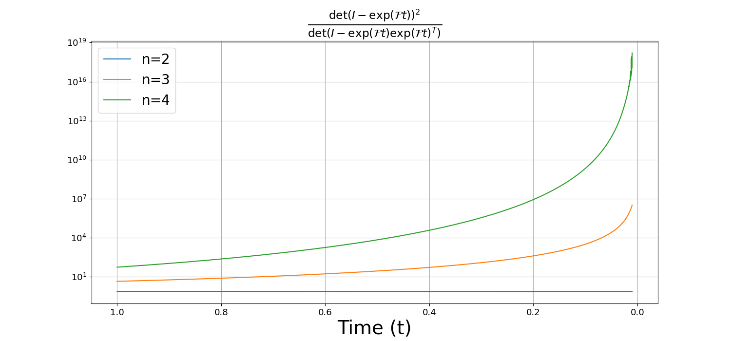
Refer to caption
Figure 2: Determinant of the inverse covariance matrix, assuming L−1=1L^{-1}=1, used to calculate the Mahalanobis distance in Proposition 2. As one raises model order, the determinant only increases, thereby improving resistance to distribution collapse.

4 Experiments

In order to validate the theory that HOLD regularizes the training and sample generation processes, we perform experiments in a setup similar to (Bonnaire et al., 2025). We compare memorization rate and generation quality along the training of HOLD diffusion models and first-order diffusion models based on the widely used Variance Preserving Stochastic Differential Equation (VPSDE) framework. Successful regularization should force memorization lower while preserving similar image qualities, measured by Fréchet Inception Distance (FID) (Heusel et al., 2017). Memorization measurement is performed on the sample level, as in (Bonnaire et al., 2025). The distances between every generated sample and every training sample are computed. For every generated sample, the gap ratio, the ratio of distances between the first closest and second closest training samples is computed. If it falls below a certain threshold, then that generated sample is declared to be memorized. Each reported memorization percentage is the ratio of memorized generated samples over the total number of generated samples in that batch.

Formally, we use a batch size B=1024B=1024 and a gap ratio threshold τ=0.333\tau=0.333 (as in (Bonnaire et al., 2025; Yoon et al., 2023; Gu et al., 2025)), and define dk(j)d^{(j)}_{k} as the ℓ2\ell_{2} distance between the kkth generated sample and the jjth closest image in the training set. The memorization metric, termed Fmem, is calculated as follows:

Mk\displaystyle M_{k} ={1,dk(1)/dk(2)<τ0,else,Fmem=1B​∑k=1BMk.\displaystyle=\begin{cases}1,\quad d^{(1)}_{k}/d^{(2)}_{k}<\tau\\ 0,\quad\text{else}\end{cases},\quad\text{Fmem}=\frac{1}{B}\sum_{k=1}^{B}M_{k}.

Confidence intervals are obtained recognizing that Fmem is a sample proportion. More experimental details appear in Appendix D.

4.1 CelebA Dataset

The main experimental setup in our paper examines the memorization behavior of HOLD throughout training on the CelebA dataset (Liu et al., 2015) for different dataset sizes. To facilitate extensive examination, before training, the images are shrunk from the center to size 32×3232\times 32, and are converted from RBG to grayscale. These are the exact same preprocessing steps that (Bonnaire et al., 2025) uses; we also use the same UNet architecture and data splits. The only architectural deviation was the additional inputs required for the auxiliary variables.

Figure 3 presents the FID and Fmem results during training for four different dataset sizes ntrainn_{\text{train}}. From inspection of this figure, HOLD orders 22 and 33 respectively improve memorization resistance for comparable FID levels at each selected ntrainn_{\text{train}}. The generated data samples in Figure 4 confirm these findings (See Appendix C for more visual results). Eight generated samples are drawn from each model and compared against their nearest neighbors in the training set. A majority the images generated by the VPSDE diffusion model either closely or identically resemble certain training data images. The HOLD n=2n=2 case significantly reduces the memorization percentage and for the most part produces images that look quite different from their nearest training neighbors. Finally HOLD n=3n=3 further improves HOLD n=2n=2 in the same fashion. Each diffusion model produces nearly equal FIDs at this number of training iterations, and visual image quality is similar overall.

Refer to caption
Figure 3: CelebA FIDs and fraction memorized (Fmem) percentages by the number of training samples. Memorization is presented with 95% confidence intervals. Using HOLD and increasing the model order helps to mitigate memorization for roughly the same FID levels.
Refer to caption
(a) VPSDE. Fmem: ​27.339%,FID: ​53.823\text{Fmem: }27.339\%,\text{FID: }53.823
Refer to caption
(b) HOLD n=2n=2. Fmem: ​4.029%,FID: ​55.819\text{Fmem: }4.029\%,\text{FID: }55.819
Refer to caption
(c) HOLD n=3n=3. Fmem: ​0.101%,FID: ​52.223\text{Fmem: }0.101\%,\text{FID: }52.223
Figure 4: Nearest training neighbors for different models at 2​e​62\mathrm{e}6 training iterations with 20482048 training images on the CelebA dataset. Each first row contains the generated images, and each second row contains the corresponding nearest neighbors. The VPSDE generated samples are heavily memorized, while the HOLD generated images, for the most part, are not nearly as memorized.

4.2 CIFAR-10 Dataset

We perform similar experiments with the same UNet architecture on the CIFAR-10 dataset (Krizhevsky et al., 2009) (converted to grayscale), and similar conclusions hold here. The key difference between CIFAR-10 and CelebA is that this dataset features ten different image categories, resulting in more dataset diversity and ultimately fewer images to learn from per category. However, this difference does not change the capabilities of HOLD that delay and attenuate memorization. Figure 5 demonstrates this, with memorization decreasing for higher orders, and plateauing to roughly the same FID. These curves do exhibit higher memorization variances and higher FIDs, but this is due to the fact that there are less images per category.

Refer to caption
Figure 5: CIFAR-10 FIDs and fraction memorized (Fmem) percentages by the number of training samples. Memorization presented with 95% confidence intervals. Using HOLD and increasing the model order helps to mitigate memorization for similar FID levels.

5 Conclusion

While diffusion models offer unparalleled generated image quality compared to earlier methods, they are also susceptible to memorization. Previous works have suggested early stopping as a solution, but when this is inconvenient to do, there are not many other techniques in the literature that are designed to prevent model memorization. The theoretical and empirical results presented in this work suggest that HOLD models may be used to perform statistical shrinkage on both the training and sampling procedures, alleviating this problem that is otherwise difficult to measure. One future point of work would be further exploration of diffusion models that implicitly act as low-pass filters on their score function. This work did not explore optimizing the forward SDE to obtain optimal filtering properties. It would be worthwhile to explore alternate models inspired by classical signal processing, and whether they could potentially further reduce memorization without compromising the generation quality.

Some limitations of HOLD are that it requires a slightly larger memory footprint. However, the number of necessary parameters do not increase by a factor of nn (the model order); in our experiments, only extra inputs were added to the network to include the auxiliary variables. It is also worth noting that n=4n=4 still achieves reasonable image qualities, but the qualities start to taper off for model orders higher than this (Sterling et al., 2025b). Regarding the broader impact of our work, reducing memorization in diffusion models is largely beneficial: when training data is used with consent, it helps protect copyright and user privacy by making such data harder to extract from the trained model. On the other hand, making diffusion models less prone to memorization may also make it harder to detect when users’ data has been used for training without their consent.

Acknowledgment

TT was supported by the Israel Science Foundation grant No. 1940/23 and MOST grant No. 0007091.

References

  • S. Abu-Hussein, T. Tirer, and R. Giryes (2022) Adir: adaptive diffusion for image reconstruction. arXiv preprint arXiv:2212.03221. Cited by: §1.
  • B. D. Anderson (1982) Reverse-time diffusion equation models. Stochastic Processes and their Applications 12 (3), pp. 313–326. Cited by: §2.1.
  • P. L. Bartlett, P. M. Long, G. Lugosi, and A. Tsigler (2020) Benign overfitting in linear regression. Proceedings of the National Academy of Sciences 117 (48), pp. 30063–30070. External Links: Document, Link, https://www.pnas.org/doi/pdf/10.1073/pnas.1907378117 Cited by: §1.
  • T. Bonnaire, R. Urfin, G. Biroli, and M. Mezard (2025) Why diffusion models don’t memorize: the role of implicit dynamical regularization in training. In The Thirty-ninth Annual Conference on Neural Information Processing Systems, External Links: Link Cited by: Appendix D, §1, §1, §2.1, §4.1, §4, §4.
  • N. Carlini, J. Hayes, M. Nasr, M. Jagielski, V. Sehwag, F. Tramer, B. Balle, D. Ippolito, and E. Wallace (2023) Extracting training data from diffusion models. In 32nd USENIX security symposium (USENIX Security 23), pp. 5253–5270. Cited by: §1.
  • T. Dockhorn, A. Vahdat, and K. Kreis (2022) Score-based generative modeling with critically-damped Langevin diffusion. In International Conference on Learning Representations, Cited by: §1, §2.2, §2.2.
  • T. Garber and T. Tirer (2024) Image restoration by denoising diffusion models with iteratively preconditioned guidance. In Proceedings of the IEEE/CVF conference on computer vision and pattern recognition, pp. 25245–25254. Cited by: §1.
  • T. Garber and T. Tirer (2025) Zero-shot image restoration using few-step guidance of consistency models (and beyond). In Proceedings of the Computer Vision and Pattern Recognition Conference, pp. 2398–2407. Cited by: §1.
  • A. J. George, R. Veiga, and N. Macris (2026) Denoising score matching with random features: insights on diffusion models from precise learning curves. In The 29th International Conference on Artificial Intelligence and Statistics, External Links: Link Cited by: §1, §2.1.
  • X. Gu, C. Du, T. Pang, C. Li, M. Lin, and Y. Wang (2025) On memorization in diffusion models. Transactions on Machine Learning Research. External Links: ISSN 2835-8856 Cited by: §1, §4.
  • M. Heusel, H. Ramsauer, T. Unterthiner, B. Nessler, and S. Hochreiter (2017) Gans trained by a two time-scale update rule converge to a local nash equilibrium. Advances in neural information processing systems 30. Cited by: §4.
  • J. Ho, A. Jain, and P. Abbeel (2020) Denoising diffusion probabilistic models. Advances in Neural Information Processing Systems 33, pp. 6840–6851. Cited by: §1.
  • Z. Kadkhodaie, F. Guth, E. P. Simoncelli, and S. Mallat (2024) Generalization in diffusion models arises from geometry-adaptive harmonic representations. In The Twelfth International Conference on Learning Representations, Cited by: §1, §2.1.
  • T. Karras, M. Aittala, T. Aila, and S. Laine (2022) Elucidating the design space of diffusion-based generative models. In Advances in Neural Information Processing Systems, A. H. Oh, A. Agarwal, D. Belgrave, and K. Cho (Eds.), External Links: Link Cited by: §1, §2.1.
  • B. Kawar, M. Elad, S. Ermon, and J. Song (2022) Denoising diffusion restoration models. Advances in neural information processing systems 35, pp. 23593–23606. Cited by: §1.
  • A. Krizhevsky, G. Hinton, et al. (2009) Learning multiple layers of features from tiny images. Cited by: §4.2.
  • Z. Liu, P. Luo, X. Wang, and X. Tang (2015) Deep learning face attributes in the wild. In Proceedings of the IEEE international conference on computer vision, pp. 3730–3738. Cited by: §4.1.
  • C. Meng, Y. He, Y. Song, J. Song, J. Wu, J. Zhu, and S. Ermon (2022) SDEdit: guided image synthesis and editing with stochastic differential equations. In International Conference on Learning Representations, Cited by: §1.
  • A. V. Oppenheim, A. S. Willsky, and S. H. Nawab (1997) Signals & systems. Pearson Educación. Cited by: §3.1.
  • E. J. Putzer (1966) Avoiding the Jordan canonical form in the discussion of linear systems with constant coefficients. The American Mathematical Monthly 73 (1), pp. 2–7. Cited by: §2.2.
  • S. Särkkä and A. Solin (2019) Applied stochastic differential equations. Vol. 10, Cambridge University Press. Cited by: §2.2.
  • Z. Shi and R. Liu (2024) Generative modelling with higher-order Langevin dynamics. arXiv preprint arXiv:2404.12814. Cited by: §1, §2.2, §2.2, §2.2.
  • J. Sohl-Dickstein, E. A. Weiss, N. Maheswaranathan, and S. Ganguli (2015) Deep unsupervised learning using nonequilibrium thermodynamics. External Links: 1503.03585 Cited by: §1.
  • G. Somepalli, V. Singla, M. Goldblum, J. Geiping, and T. Goldstein (2023) Diffusion art or digital forgery? investigating data replication in diffusion models. In Proceedings of the IEEE/CVF conference on computer vision and pattern recognition, pp. 6048–6058. Cited by: §1.
  • Y. Song and S. Ermon (2019) Generative modeling by estimating gradients of the data distribution. Advances in neural information processing systems 32. Cited by: §1.
  • Y. Song, J. Sohl-Dickstein, D. P. Kingma, A. Kumar, S. Ermon, and B. Poole (2021) Score-based generative modeling through stochastic differential equations. In International Conference on Learning Representations, External Links: Link Cited by: §1, §2.1, §2.2.
  • B. Sterling and M. F. Bugallo (2025) Critically-damped third-order Langevin dynamics. In ICASSP 2025 - 2025 IEEE International Conference on Acoustics, Speech and Signal Processing (ICASSP), Vol. , pp. 1–5. External Links: Document Cited by: §1.
  • B. Sterling, Y. El-Laham, and M. F. Bugallo (2025a) Defending diffusion models against membership inference attacks via higher-order Langevin dynamics. External Links: 2509.14225, Link Cited by: §1.
  • B. Sterling, C. Gueli, and M. F. Bugallo (2025b) Critically-damped higher-order Langevin dynamics. External Links: 2506.21741, Link Cited by: §1, §2.2, §2.2, §2.2, §2.2, §3.1, §5.
  • M. Yi, J. Sun, and Z. Li (2023) On the generalization of diffusion model. arXiv preprint arXiv:2305.14712. Cited by: §1, §2.1.
  • T. Yoon, J. Y. Choi, S. Kwon, and E. K. Ryu (2023) Diffusion probabilistic models generalize when they fail to memorize. In ICML 2023 Workshop on Structured Probabilistic Inference & Generative Modeling, Cited by: §1, §4.
  • H. Zhang, J. Zhou, Y. Lu, M. Guo, P. Wang, L. Shen, and Q. Qu (2024) The emergence of reproducibility and consistency in diffusion models. In Forty-first International Conference on Machine Learning, Cited by: §1, §2.1.

Appendix A Technical Proofs

This section of the appendix will be used to rigorously prove the theoretical claims of paper.

A.1 Proof of Proposition 1

Proof.

Start with training samples {𝐮0(k)},1≤k≤ntrain\{\mathbf{u}_{0}^{(k)}\},1\leq k\leq n_{\text{train}}. The data distribution, including initial auxiliary variables, may be expressed as the following linear combinations of Dirac delta distributions:

pdata​(𝐮)\displaystyle p_{\text{data}}(\mathbf{u}) =1ntrain​∑k=1ntrainδ​(𝐮−𝐮0(k))\displaystyle=\frac{1}{n_{\text{train}}}\sum_{k=1}^{n_{\text{train}}}\delta(\mathbf{u}-\mathbf{u}_{0}^{(k)})
ℒ​(sθ)\displaystyle\mathcal{L}(s_{\theta}) =𝔼t∼𝒰​(0,1),𝐮0,ϵfull​‖ϵn+𝐬θ​(𝐮t,t)​(𝐋t​[n​h,n​h])‖2\displaystyle=\mathbb{E}_{t\sim\mathcal{U}(0,1),\mathbf{u}_{0},\boldsymbol{\epsilon}_{\text{full}}}||\boldsymbol{\epsilon}_{n}+\mathbf{s}_{\theta}(\mathbf{u}_{t},t)\left(\mathbf{L}_{t}[nh,nh]\right)||^{2}
=∫𝔼t∼𝒰​(0,1),𝐮0​‖ϵn+𝐬θ​(𝐮t,t)​(𝐋t​[n​h,n​h])‖2​p​(ϵfull)​𝑑ϵfull=∫ℒ​(sθ,𝐮t)​𝑑ϵfull.\displaystyle=\int\mathbb{E}_{t\sim\mathcal{U}(0,1),\mathbf{u}_{0}}||\boldsymbol{\epsilon}_{n}+\mathbf{s}_{\theta}(\mathbf{u}_{t},t)\left(\mathbf{L}_{t}[nh,nh]\right)||^{2}p(\boldsymbol{\epsilon}_{\text{full}})d\boldsymbol{\epsilon}_{\text{full}}=\int\mathcal{L}(s_{\theta},\mathbf{u}_{t})d\boldsymbol{\epsilon}_{\text{full}}.

Minimizing ℒ​(sθ)\mathcal{L}(s_{\theta}) may be achieved by minimizing ℒ​(sθ,𝐮t)\mathcal{L}(s_{\theta},\mathbf{u}_{t}) instead. We do this by minimizing this loss over all 𝐬θ\mathbf{s}_{\theta} as follows. We define ϵfull(k)=𝐋t−1​(𝐮t−exp⁡(ℱ​t)​𝐮0(k))\boldsymbol{\epsilon}_{\text{full}}^{(k)}=\mathbf{L}_{t}^{-1}\left(\mathbf{u}_{t}-\exp(\mathcal{F}t)\mathbf{u}_{0}^{(k)}\right) and ϵn(k)=[ϵfull(k)]n​(h−1):n​h\boldsymbol{\epsilon}_{n}^{(k)}=\left[\boldsymbol{\epsilon}^{(k)}_{\text{full}}\right]_{n(h-1):nh}; that is the final n entries of the vector ϵfull(k\boldsymbol{\epsilon}^{(k}_{\text{full}}. Both come from the kkth sample.

ℒ​(𝐬θ,𝐮t)\displaystyle\mathcal{L}(\mathbf{s}_{\theta},\mathbf{u}_{t}) =1ntrain​∑k=1ntrain‖ϵn(k)+𝐬θ​(𝐮t,t)​(𝐋t​[n​h,n​h])‖2​p​(ϵfull(k)).\displaystyle=\frac{1}{n_{\text{train}}}\sum_{k=1}^{n_{\text{train}}}||\boldsymbol{\epsilon}^{(k)}_{n}+\mathbf{s}_{\theta}(\mathbf{u}_{t},t)\left(\mathbf{L}_{t}[nh,nh]\right)||^{2}p(\boldsymbol{\epsilon}_{\text{full}}^{(k)}).

Take the gradient with respect to 𝐬θ\mathbf{s}_{\theta} and set it to zero:

∑k=1ntrain(ϵn(k)+𝐬θ​(𝐮t,t)​(𝐋t​[n​h,n​h]))​p​(ϵfull(k))=0\displaystyle\sum_{k=1}^{n_{\text{train}}}\left(\boldsymbol{\epsilon}^{(k)}_{n}+\mathbf{s}_{\theta}(\mathbf{u}_{t},t)\left(\mathbf{L}_{t}[nh,nh]\right)\right)p(\boldsymbol{\epsilon}_{\text{full}}^{(k)})=0
𝐬θ​(𝐮t,t)=−∑k=1ntrainp​(ϵfull(k))​ϵn(k)/𝐋t​[n​h,n​h]∑k=1ntrainp​(ϵfull(k))=∑k=1ntrainp​(ϵfull(k))​∇𝐯t(n−1)log⁡p​(𝐮t∣𝐮0(k))∑k=1ntrainp​(ϵfull(k))\displaystyle\mathbf{s}_{\theta}(\mathbf{u}_{t},t)=-\frac{\sum_{k=1}^{n_{\text{train}}}p(\boldsymbol{\epsilon}^{(k)}_{\text{full}})\boldsymbol{\epsilon}_{n}^{(k)}/\mathbf{L}_{t}[nh,nh]}{\sum_{k=1}^{n_{\text{train}}}p(\boldsymbol{\epsilon}^{(k)}_{\text{full}})}=\frac{\sum_{k=1}^{n_{\text{train}}}p(\boldsymbol{\epsilon}^{(k)}_{\text{full}})\nabla_{\mathbf{v}^{(n-1)}_{t}}\log p(\mathbf{u}_{t}\mid\mathbf{u}^{(k)}_{0})}{\sum_{k=1}^{n_{\text{train}}}p(\boldsymbol{\epsilon}^{(k)}_{\text{full}})}
=[∑k=1ntrainp​(ϵfull(k))​∇𝐮tlog⁡p​(𝐮t∣𝐮0(k))∑k=1ntrainp​(ϵfull(k))]n​(h−1):n​h.\displaystyle=\left[\frac{\sum_{k=1}^{n_{\text{train}}}p(\boldsymbol{\epsilon}^{(k)}_{\text{full}})\nabla_{\mathbf{u}_{t}}\log p(\mathbf{u}_{t}\mid\mathbf{u}^{(k)}_{0})}{\sum_{k=1}^{n_{\text{train}}}p(\boldsymbol{\epsilon}^{(k)}_{\text{full}})}\right]_{n(h-1):nh}.

If one calculates the score function corresponding to ptempp_{t}^{\text{emp}}, then it follows that 𝐬θ​(𝐮t,t)=[∇𝐮tlog⁡ptemp​(𝐮t)]n​(h−1):n​h\mathbf{s}_{\theta}(\mathbf{u}_{t},t)=\left[\nabla_{\mathbf{u}_{t}}\log p^{\text{emp}}_{t}(\mathbf{u}_{t})\right]_{n(h-1):nh}. ∎

A.2 Proof of Lemma 1

Proof.

Note that 𝐮~​(s)=vec⁡(𝐱~​(s),𝐯~(1)​(s),…​𝐯~(n−1)​(s)),𝐒~​(s)=𝐒θ​(𝐮t,t)\tilde{\mathbf{u}}(s)=\operatorname{vec}(\tilde{\mathbf{x}}(s),\tilde{\mathbf{v}}^{(1)}(s),\ldots\tilde{\mathbf{v}}^{(n-1)}(s)),\tilde{\mathbf{S}}(s)=\mathbf{S}_{\theta}(\mathbf{u}_{t},t).

d​𝐮td​t\displaystyle\frac{d\mathbf{u}_{t}}{dt} =ℱ​𝐮t−ξ​L−1​𝐄n,n​𝐒θ​(𝐮t,t)\displaystyle=\mathcal{F}\mathbf{u}_{t}-\xi L^{-1}\mathbf{E}_{n,n}\mathbf{S}_{\theta}(\mathbf{u}_{t},t)
s​𝐮~​(s)−𝐮0\displaystyle s\tilde{\mathbf{u}}(s)-\mathbf{u}_{0} =ℱ​𝐮~​(s)−ξ​L−1​𝐄n,n​𝐒~​(s)\displaystyle=\mathcal{F}\tilde{\mathbf{u}}(s)-\xi L^{-1}\mathbf{E}_{n,n}\tilde{\mathbf{S}}(s)
((𝐅−s​𝐈)⊗𝐈h)​𝐮~​(s)\displaystyle((\mathbf{F}-s\mathbf{I})\otimes\mathbf{I}_{h})\tilde{\mathbf{u}}(s) =ξ​L−1​𝐄n,n​𝐒~​(s)−𝐮0.\displaystyle=\xi L^{-1}\mathbf{E}_{n,n}\tilde{\mathbf{S}}(s)-\mathbf{u}_{0}.

Now, use Cramer’s Rule to solve for 𝐱~​(s)\tilde{\mathbf{x}}(s). Take 𝟎,𝟏∈ℝh\mathbf{0},\mathbf{1}\in\mathbb{R}^{h} as the vector of all zeros and ones respectively. blockdet\mathrm{blockdet} takes determinants across each coordinate of the following vectors and returns them in a single vector. P​(s)=det(𝐅−s​𝐈)P(s)=\det(\mathbf{F}-s\mathbf{I}) is the characteristic polynomial of 𝐅\mathbf{F}. The second line follows from the multilinearity of the determinant.

𝐱~​(s)\displaystyle\tilde{\mathbf{x}}(s) =1P​(s)​blockdet​(−𝐱0γ1​𝟏…𝟎−𝐯0(1)−s​𝟏…𝟎…………−𝐯0(n−2)…−s​𝟏γn−1​𝟏ξ​L−1​𝐬~​(s)−𝐯0(n−1)…−γn−1​𝟏(−s−ξ)​𝟏)\displaystyle=\frac{1}{P(s)}\mathrm{blockdet}\begin{pmatrix}-\mathbf{x}_{0}&\gamma_{1}\mathbf{1}&\ldots&\mathbf{0}\\ -\mathbf{v}^{(1)}_{0}&-s\mathbf{1}&\ldots&\mathbf{0}\\ \ldots&\ldots&\ldots&\ldots\\ -\mathbf{v}^{(n-2)}_{0}&\ldots&-s\mathbf{1}&\gamma_{n-1}\mathbf{1}\\ \xi L^{-1}\tilde{\mathbf{s}}(s)-\mathbf{v}^{(n-1)}_{0}&\ldots&-\gamma_{n-1}\mathbf{1}&(-s-\xi)\mathbf{1}\end{pmatrix}
=ξ​L−1P​(s)​blockdet​(𝟎γ1​𝟏…𝟎𝟎−s​𝟏…𝟎…………𝟎…−s​𝟏γn−1​𝟏𝐬~​(s)…−γn−1​𝟏(−s−ξ)​𝟏)\displaystyle=\frac{\xi L^{-1}}{P(s)}\mathrm{blockdet}\begin{pmatrix}\mathbf{0}&\gamma_{1}\mathbf{1}&\ldots&\mathbf{0}\\ \mathbf{0}&-s\mathbf{1}&\ldots&\mathbf{0}\\ \ldots&\ldots&\ldots&\ldots\\ \mathbf{0}&\ldots&-s\mathbf{1}&\gamma_{n-1}\mathbf{1}\\ \tilde{\mathbf{s}}(s)&\ldots&-\gamma_{n-1}\mathbf{1}&(-s-\xi)\mathbf{1}\end{pmatrix}
+1P​(s)​blockdet​(−𝐱0γ1​𝟏…𝟎−𝐯0(1)−s​𝟏…𝟎…………−𝐯0(n−2)…−s​𝟏γn−1​𝟏−𝐯0(n−1)…−γn−1​𝟏(−s−ξ)​𝟏)\displaystyle+\frac{1}{P(s)}\mathrm{blockdet}\begin{pmatrix}-\mathbf{x}_{0}&\gamma_{1}\mathbf{1}&\ldots&\mathbf{0}\\ -\mathbf{v}^{(1)}_{0}&-s\mathbf{1}&\ldots&\mathbf{0}\\ \ldots&\ldots&\ldots&\ldots\\ -\mathbf{v}^{(n-2)}_{0}&\ldots&-s\mathbf{1}&\gamma_{n-1}\mathbf{1}\\ -\mathbf{v}^{(n-1)}_{0}&\ldots&-\gamma_{n-1}\mathbf{1}&(-s-\xi)\mathbf{1}\end{pmatrix}
=(−1)n−1​ξ​L−1​𝐬~​(s)P​(s)​det(γ10…0−sγ2…0……………0−sγn−1)+𝐱~natural​(s)\displaystyle=\frac{(-1)^{n-1}\xi L^{-1}\tilde{\mathbf{s}}(s)}{P(s)}\det\begin{pmatrix}\gamma_{1}&0&\ldots&0\\ -s&\gamma_{2}&\ldots&0\\ \ldots&\ldots&\ldots&\ldots\\ \ldots&0&-s&\gamma_{n-1}\end{pmatrix}+\tilde{\mathbf{x}}^{\text{natural}}(s)
𝐱~​(s)\displaystyle\tilde{\mathbf{x}}(s) =−γ¯​ξ​L−1​𝐬~​(s)P​(s)+𝐱~natural​(s).\displaystyle=-\frac{\bar{\gamma}\xi L^{-1}\tilde{\mathbf{s}}(s)}{P(s)}+\tilde{\mathbf{x}}^{\text{natural}}(s).

where 𝐱~natural​(s)\tilde{\mathbf{x}}^{\mathrm{natural}}(s) is given by:

𝐱~natural​(s)=1P​(s)​blockdet​(−𝐱0γ1​𝟏…𝟎−𝐯0(1)−s​𝟏…𝟎…………−𝐯0(n−2)…−s​𝟏γn−1​𝟏−𝐯0(n−1)…−γn−1​𝟏(−s−ξ)​𝟏).\tilde{\mathbf{x}}^{\mathrm{natural}}(s)=\frac{1}{P(s)}\mathrm{blockdet}\begin{pmatrix}-\mathbf{x}_{0}&\gamma_{1}\mathbf{1}&\ldots&\mathbf{0}\\ -\mathbf{v}^{(1)}_{0}&-s\mathbf{1}&\ldots&\mathbf{0}\\ \ldots&\ldots&\ldots&\ldots\\ -\mathbf{v}^{(n-2)}_{0}&\ldots&-s\mathbf{1}&\gamma_{n-1}\mathbf{1}\\ -\mathbf{v}^{(n-1)}_{0}&\ldots&-\gamma_{n-1}\mathbf{1}&(-s-\xi)\mathbf{1}\end{pmatrix}.

The last determinant is simply the product of gammas because the matrice’s main diagonal contains the gammas, and one minor row filled with −s-s. Note that the negative characteristic polynomial is also a valid characteristic polynomial, but we take the polynomial with a leading positive coefficient. ∎

A.3 Proof of Theorem 1

Proof.

According to Lemma 1,

𝐱~​(s)\displaystyle\tilde{\mathbf{x}}(s) =−γ¯​ξ​L−1​𝐬~​(s)(s−s∗)n+𝐱~natural​(s).\displaystyle=-\frac{\bar{\gamma}\xi L^{-1}\tilde{\mathbf{s}}(s)}{(s-s_{*})^{n}}+\tilde{\mathbf{x}}^{\text{natural}}(s).

This equation assumes that we use the critically-damped parameter selection. Further define H​(s)=−γ¯​ξ​L−1(s−s∗)nH(s)=-\frac{\bar{\gamma}\xi L^{-1}}{(s-s_{*})^{n}}. To solve for hth_{t}, we must take the inverse Laplace transform:

ht\displaystyle h_{t} =12​π​i​limT→∞∫γ−i​Tγ+i​TH​(s)​exp⁡(s​t)​𝑑s\displaystyle=\frac{1}{2\pi i}\lim_{T\to\infty}\int_{\gamma-iT}^{\gamma+iT}H(s)\exp(st)ds

for some γ>0\gamma>0. Now we utilize the Residue Theorem:

ht\displaystyle h_{t} =Res⁡(H​(s)​exp⁡(s​t))∣s=s∗\displaystyle=\operatorname{Res}(H(s)\exp(st))\mid_{s=s_{*}}
=lims→s∗dn−1d​sn−1​(H​(s)​exp⁡(s​t)​(s−s∗)n)\displaystyle=\lim_{s\to s_{*}}\frac{d^{n-1}}{ds^{n-1}}\left(H(s)\exp(st)(s-s_{*})^{n}\right)
=−γ¯​ξ​L−1​lims→s∗dn−1d​sn−1​(exp⁡(s​t))\displaystyle=-\bar{\gamma}\xi L^{-1}\lim_{s\to s_{*}}\frac{d^{n-1}}{ds^{n-1}}\left(\exp(st)\right)
=−γ¯​ξ​L−1​tn−1​exp⁡(s∗​t)=−γ¯​n​2​n−3​L−1​tn−1​exp⁡(−t​2​n−3).\displaystyle=-\bar{\gamma}\xi L^{-1}t^{n-1}\exp(s_{*}t)=-\bar{\gamma}n\sqrt{2n-3}L^{-1}t^{n-1}\exp(-t\sqrt{2n-3}).

Finally, the Convolution Theorem applied to 𝐱~​(s)=H​(s)​𝐬~​(s)+𝐱~natural​(s)\tilde{\mathbf{x}}(s)=H(s)\tilde{\mathbf{s}}(s)+\tilde{\mathbf{x}}^{\text{natural}}(s) proves the theorem. ∎

A.4 Proof of Proposition 2

Proof.
ptemp, HOLD\displaystyle p^{\text{emp, HOLD}}_{t} ≈𝒩(𝝁tOU,𝚺tHOLD)=𝒩(exp(ℱt)𝐮0(k),L−1(𝐈−exp(ℱt)exp(ℱt)T)),\displaystyle\approx\mathcal{N}(\boldsymbol{\mu}^{\text{OU}}_{t},\boldsymbol{\Sigma}^{\text{HOLD}}_{t})=\mathcal{N}(\exp(\mathcal{F}t)\mathbf{u}^{(k)}_{0},L^{-1}(\mathbf{I}-\exp(\mathcal{F}t)\exp(\mathcal{F}t)^{T})),
ptemp, OU\displaystyle p^{\text{emp, OU}}_{t} ≈𝒩​(𝝁tOU,𝚺tOU)=𝒩​(exp⁡(−ξ​t)​𝐱0(k),L−1​(1−exp⁡(−2​ξ​t))​𝐈).\displaystyle\approx\mathcal{N}(\boldsymbol{\mu}^{\text{OU}}_{t},\boldsymbol{\Sigma}^{\text{OU}}_{t})=\mathcal{N}(\exp(-\xi t)\mathbf{x}^{(k)}_{0},L^{-1}(1-\exp(-2\xi t))\mathbf{I}).

One may formally calculate that the Mahalanobis distance for the Ornstein–Uhlenbeck diffusion process is zero. Use L’Hôpital’s rule to solve the final limit.

DM​(𝐱0(k),ptemp, OU)2\displaystyle D_{M}(\mathbf{x}^{(k)}_{0},p^{\text{emp, OU}}_{t})^{2} =(𝐱0(k)−exp⁡(−ξ​t)​𝐱0(k))T​𝐈L−1​(1−exp⁡(−2​ξ​t))​(𝐱0(k)−exp⁡(−ξ​t)​𝐱0(k))\displaystyle=(\mathbf{x}^{(k)}_{0}-\exp(-\xi t)\mathbf{x}^{(k)}_{0})^{T}\frac{\mathbf{I}}{L^{-1}(1-\exp(-2\xi t))}(\mathbf{x}^{(k)}_{0}-\exp(-\xi t)\mathbf{x}^{(k)}_{0})
=(1−exp⁡(−ξ​t))2L−1​(1−exp⁡(−2​ξ​t))​‖𝐱0(k)‖2,\displaystyle=\frac{(1-\exp(-\xi t))^{2}}{L^{-1}(1-\exp(-2\xi t))}||\mathbf{x}^{(k)}_{0}||^{2},
limt→0+DM​(𝐱0(k),ptemp, OU)2\displaystyle\lim_{t\to 0^{+}}D_{M}(\mathbf{x}^{(k)}_{0},p^{\text{emp, OU}}_{t})^{2} =limt→0+(1−exp⁡(−ξ​t))2L−1​(1−exp⁡(−2​ξ​t))​‖𝐱0(k)‖2=0.\displaystyle=\lim_{t\to 0^{+}}\frac{(1-\exp(-\xi t))^{2}}{L^{-1}(1-\exp(-2\xi t))}||\mathbf{x}^{(k)}_{0}||^{2}=0.

However, this limit is different for HOLD:

DM​(𝐮0(k),ptemp, HOLD)2\displaystyle D_{M}(\mathbf{u}^{(k)}_{0},p^{\text{emp, HOLD}}_{t})^{2} =1L−1(𝐮0(k)−exp(ℱt)𝐮0(k))T(𝐈−exp(ℱt)exp(ℱt)T)−1(𝐮0(k)−exp(ℱt)𝐮0(k))\displaystyle=\frac{1}{L^{-1}}(\mathbf{u}^{(k)}_{0}-\exp(\mathcal{F}t)\mathbf{u}^{(k)}_{0})^{T}\left(\mathbf{I}-\exp(\mathcal{F}t)\exp(\mathcal{F}t)^{T}\right)^{-1}(\mathbf{u}^{(k)}_{0}-\exp(\mathcal{F}t)\mathbf{u}^{(k)}_{0})
=1L−1(𝐮0(k))T(𝐈−exp(ℱt)T)(𝐈−exp(ℱt)exp(ℱt)T)−1(𝐈−exp(ℱt))𝐮0(k).\displaystyle=\frac{1}{L^{-1}}(\mathbf{u}^{(k)}_{0})^{T}(\mathbf{I}-\exp(\mathcal{F}t)^{T})\left(\mathbf{I}-\exp(\mathcal{F}t)\exp(\mathcal{F}t)^{T}\right)^{-1}(\mathbf{I}-\exp(\mathcal{F}t))\mathbf{u}^{(k)}_{0}.

We are interested in the limit behavior as t→0+t\to 0^{+}. To analyze it, take the limit of the determinant of the inverse covariance matrix in the middle. For the purposes of this determinant, use 𝐅\mathbf{F} instead of ℱ=𝐅⊗𝐈h\mathcal{F}=\mathbf{F}\otimes\mathbf{I}_{h}. The proof works out identically since for any matrix 𝐀∈ℝn×n\mathbf{A}\in\mathbb{R}^{n\times n}, exp⁡(𝐀⊗𝐈h)=exp⁡(𝐀)⊗𝐈h\exp(\mathbf{A}\otimes\mathbf{I}_{h})=\exp(\mathbf{A})\otimes\mathbf{I}_{h}, and det(𝐀⊗𝐈h)=det(𝐀)h\det(\mathbf{A}\otimes\mathbf{I}_{h})=\det(\mathbf{A})^{h}; this does not change the determinant’s behavior as we mainly care whether it goes to zero, remains finite, or diverges to infinity.

limt→0+det((𝐈−exp(𝐅t)T)(𝐈−exp(𝐅t)exp(𝐅t)T)−1(𝐈−exp(𝐅t)))\displaystyle\lim_{t\to 0^{+}}\det\left((\mathbf{I}-\exp(\mathbf{F}t)^{T})\left(\mathbf{I}-\exp(\mathbf{F}t)\exp(\mathbf{F}t)^{T}\right)^{-1}(\mathbf{I}-\exp(\mathbf{F}t))\right)
=limt→0+det(𝐈−exp⁡(𝐅​t))2det(𝐈−exp(𝐅t)exp(𝐅t)T).\displaystyle=\lim_{t\to 0^{+}}\frac{\det(\mathbf{I}-\exp(\mathbf{F}t))^{2}}{\det(\mathbf{I}-\exp(\mathbf{F}t)\exp(\mathbf{F}t)^{T})}.

Firstly, a property of determinants is that it is the product of the eigenvalues of the argument. The eigenvalues of 𝐈−exp⁡(𝐅​t)\mathbf{I}-\exp(\mathbf{F}t) are all 1−exp⁡(s∗​t)1-\exp(s_{*}t), therefore det(𝐈−exp⁡(𝐅​t))=(1−exp⁡(s∗​t))n\det(\mathbf{I}-\exp(\mathbf{F}t))=(1-\exp(s_{*}t))^{n}. Furthermore, as t→0+t\to 0^{+}:

(1−exp⁡(s∗​t))n\displaystyle(1-\exp(s_{*}t))^{n} =(1−(1−s∗​t+𝒪​(t2)))n=(s∗​t+𝒪​(t2))n=(s∗​t)n+𝒪​(tn+1)\displaystyle=(1-(1-s_{*}t+\mathcal{O}(t^{2})))^{n}=(s_{*}t+\mathcal{O}(t^{2}))^{n}=(s_{*}t)^{n}+\mathcal{O}(t^{n+1})
det(𝐈−exp⁡(𝐅​t))2\displaystyle\det(\mathbf{I}-\exp(\mathbf{F}t))^{2} =(s∗​t)2​n+𝒪​(t2​n+1)=(2​n−3)n​t2​n+𝒪​(t2​n+1).\displaystyle=(s_{*}t)^{2n}+\mathcal{O}(t^{2n+1})=(2n-3)^{n}t^{2n}+\mathcal{O}(t^{2n+1}).

A.4.1 Case n=2n=2

Specifically for n=2n=2, by Equation (4), exp⁡(𝐅​t)=exp⁡(−t)​(𝐈+(𝐅−s∗​𝐈)​t)\exp(\mathbf{F}t)=\exp(-t)\left(\mathbf{I}+(\mathbf{F}-s_{*}\mathbf{I})t\right), and s∗=−1,ξ=2s_{*}=-1,\xi=2. Therefore

det(𝐈−exp⁡(𝐅​t))\displaystyle\det(\mathbf{I}-\exp(\mathbf{F}t)) =(1−exp⁡(−t))2=(1−(1−t+𝒪​(t2)))2=(t+𝒪​(t2))2=t2+𝒪​(t3)\displaystyle=(1-\exp(-t))^{2}=(1-(1-t+\mathcal{O}(t^{2})))^{2}=(t+\mathcal{O}(t^{2}))^{2}=t^{2}+\mathcal{O}(t^{3})
det(𝐈−exp⁡(𝐅​t))2\displaystyle\det(\mathbf{I}-\exp(\mathbf{F}t))^{2} =t4+𝒪​(t5).\displaystyle=t^{4}+\mathcal{O}(t^{5}).

Now moving onto the denominator.

exp⁡(𝐅​t)\displaystyle\exp(\mathbf{F}t) =exp⁡(−t)​(𝐈​(1+t)+𝐅​t)\displaystyle=\exp(-t)(\mathbf{I}(1+t)+\mathbf{F}t)
=exp⁡(−t)​(1+t−tt1−t)\displaystyle=\exp(-t)\begin{pmatrix}1+t&-t\\ t&1-t\end{pmatrix}
exp(𝐅t)exp(𝐅t)T\displaystyle\exp(\mathbf{F}t)\exp(\mathbf{F}t)^{T} =exp⁡(−2​t)​(1+t−tt1−t)​(1+tt−t1−t)\displaystyle=\exp(-2t)\begin{pmatrix}1+t&-t\\ t&1-t\end{pmatrix}\begin{pmatrix}1+t&t\\ -t&1-t\end{pmatrix}
=exp⁡(−2​t)​(2​t2+2​t+12​t22​t22​t2−2​t+1)\displaystyle=\exp(-2t)\begin{pmatrix}2t^{2}+2t+1&2t^{2}\\ 2t^{2}&2t^{2}-2t+1\end{pmatrix}
𝐈−exp(𝐅t)exp(𝐅t)T\displaystyle\mathbf{I}-\exp(\mathbf{F}t)\exp(\mathbf{F}t)^{T} =(1−exp⁡(−2​t)​(2​t2+2​t+1)−2​t2​exp⁡(−2​t)−2​t2​exp⁡(−2​t)1−exp⁡(−2​t)​(2​t2−2​t+1))\displaystyle=\begin{pmatrix}1-\exp(-2t)(2t^{2}+2t+1)&-2t^{2}\exp(-2t)\\ -2t^{2}\exp(-2t)&1-\exp(-2t)(2t^{2}-2t+1)\end{pmatrix}
det(𝐈−exp(𝐅t)exp(𝐅t)T)\displaystyle\det(\mathbf{I}-\exp(\mathbf{F}t)\exp(\mathbf{F}t)^{T}) =(1−exp⁡(−2​t)​(2​t2+2​t+1))​(1−exp⁡(−2​t)​(2​t2−2​t+1))−4​t4​exp⁡(−4​t).\displaystyle=(1-\exp(-2t)(2t^{2}+2t+1))(1-\exp(-2t)(2t^{2}-2t+1))-4t^{4}\exp(-4t).

Take the rest in pieces. 4​t4​exp⁡(−4​t)=4​t4+𝒪​(t5)4t^{4}\exp(-4t)=4t^{4}+\mathcal{O}(t^{5}), and

1−exp⁡(−2​t)​(2​t2+2​t+1)\displaystyle 1-\exp(-2t)(2t^{2}+2t+1) =1−(1−2​t+2​t2−8​t36+𝒪​(t4))​(2​t2+2​t+1)\displaystyle=1-(1-2t+2t^{2}-\frac{8t^{3}}{6}+\mathcal{O}(t^{4}))(2t^{2}+2t+1)
=1−(2​t2+2​t+1)+2​t​(2​t2+2​t+1)−2​t2​(2​t2+2​t+1)+8​t36+𝒪​(t4)\displaystyle=1-(2t^{2}+2t+1)+2t(2t^{2}+2t+1)-2t^{2}(2t^{2}+2t+1)+\frac{8t^{3}}{6}+\mathcal{O}(t^{4})
=4​t33+𝒪​(t4)\displaystyle=\frac{4t^{3}}{3}+\mathcal{O}(t^{4})
1−exp⁡(−2​t)​(2​t2−2​t+1)\displaystyle 1-\exp(-2t)(2t^{2}-2t+1) =1−(1−2​t+2​t2+𝒪​(t3))​(2​t2−2​t+1)\displaystyle=1-(1-2t+2t^{2}+\mathcal{O}(t^{3}))(2t^{2}-2t+1)
=1−(2​t2−2​t+1+4​t2−2​t+2​t2+𝒪​(t3))\displaystyle=1-\left(2t^{2}-2t+1+4t^{2}-2t+2t^{2}+\mathcal{O}(t^{3})\right)
=−2​t2+2​t−4​t2+2​t−2​t2+𝒪​(t3)\displaystyle=-2t^{2}+2t-4t^{2}+2t-2t^{2}+\mathcal{O}(t^{3})
=4​t+𝒪​(t2).\displaystyle=4t+\mathcal{O}(t^{2}).

Finally, one may derive:

limt→0+det(𝐈−exp⁡(𝐅​t))2det(𝐈−exp(𝐅t)exp(𝐅t)T)\displaystyle\lim_{t\to 0^{+}}\frac{\det(\mathbf{I}-\exp(\mathbf{F}t))^{2}}{\det(\mathbf{I}-\exp(\mathbf{F}t)\exp(\mathbf{F}t)^{T})} =limt→0+t44​t33​4​t−4​t4=34.\displaystyle=\lim_{t\to 0^{+}}\frac{t^{4}}{\frac{4t^{3}}{3}4t-4t^{4}}=\frac{3}{4}.

The inverse covariance matrix is therefore positive definite as t→0+t\to 0^{+}, so limt→0+DM​(𝐮0(k),ptemp, HOLD)≫0\lim_{t\to 0^{+}}D_{M}(\mathbf{u}^{(k)}_{0},p^{\text{emp, HOLD}}_{t})\gg 0. ∎

A.4.2 Case n=3n=3

exp⁡(𝐅​t)\displaystyle\exp(\mathbf{F}t) =exp⁡(−t​3)​(t2+t​3+1t2​3+tt2​2−t2​3−t−3​t2+t​3+1−t2​6+2​t​2t2​2t2​6−2​t​22​t2−2​t​3+1)\displaystyle=\exp(-t\sqrt{3})\begin{pmatrix}t^{2}+t\sqrt{3}+1&t^{2}\sqrt{3}+t&t^{2}\sqrt{2}\\ -t^{2}\sqrt{3}-t&-3t^{2}+t\sqrt{3}+1&-t^{2}\sqrt{6}+2t\sqrt{2}\\ t^{2}\sqrt{2}&t^{2}\sqrt{6}-2t\sqrt{2}&2t^{2}-2t\sqrt{3}+1\end{pmatrix}
(1−exp⁡(−3​t))3\displaystyle(1-\exp(-\sqrt{3}t))^{3} =(1−(1−3​t+𝒪​(t2)))3=(3​t+𝒪​(t2))3=33/2​t3+𝒪​(t4)\displaystyle=(1-(1-\sqrt{3}t+\mathcal{O}(t^{2})))^{3}=(\sqrt{3}t+\mathcal{O}(t^{2}))^{3}=3^{3/2}t^{3}+\mathcal{O}(t^{4})
det(𝐈−exp⁡(𝐅​t))2\displaystyle\det(\mathbf{I}-\exp(\mathbf{F}t))^{2} =(1−exp⁡(−3​t))6=(33/2​t3+𝒪​(t4))2=27​t6+𝒪​(t7).\displaystyle=(1-\exp(-\sqrt{3}t))^{6}=(3^{3/2}t^{3}+\mathcal{O}(t^{4}))^{2}=27t^{6}+\mathcal{O}(t^{7}).

The following was computed with python’s sympy library:

det(𝐈−exp(𝐅t)exp(𝐅t)T)\displaystyle\det(\mathbf{I}-\exp(\mathbf{F}t)\exp(\mathbf{F}t)^{T}) =((−36t4+243t3−36t2−3)exp(43t)\displaystyle=\bigg((-36t^{4}+24\sqrt{3}t^{3}-36t^{2}-3)\exp(4\sqrt{3}t)
+(36t4+243t3+36t2+3)exp(23t)+exp(63t)−1)exp(−63t)\displaystyle+(36t^{4}+24\sqrt{3}t^{3}+36t^{2}+3)\exp(2\sqrt{3}t)+\exp(6\sqrt{3}t)-1\bigg)\exp(-6\sqrt{3}t)
=24​35​t9+𝒪​(t10)\displaystyle=\frac{24\sqrt{3}}{5}t^{9}+\mathcal{O}(t^{10})
limt→0+det(𝐈−exp⁡(𝐅​t))2det(𝐈−exp(𝐅t)exp(𝐅t)T)=limt→0+27​t624​35​t9→∞.\displaystyle\lim_{t\to 0^{+}}\frac{\det(\mathbf{I}-\exp(\mathbf{F}t))^{2}}{\det(\mathbf{I}-\exp(\mathbf{F}t)\exp(\mathbf{F}t)^{T})}=\lim_{t\to 0^{+}}\frac{27t^{6}}{\frac{24\sqrt{3}}{5}t^{9}}\to\infty.

The determinant of the inverse covariance matrix grows infinitely large as t→0+t\to 0^{+}, so limt→0+DM​(𝐮0(k),ptemp, HOLD)→∞\lim_{t\to 0^{+}}D_{M}(\mathbf{u}^{(k)}_{0},p^{\text{emp, HOLD}}_{t})\to\infty.

A.5 Derivation of Ornstein–Uhlenbeck Convolution

The Ornstein–Uhlenbeck convolution formula is derived from the deterministic ODE as follows

d​𝐱t\displaystyle d\mathbf{x}_{t} =(−ξ​𝐱t−2​ξ​L−12​𝐬θ​(𝐱t,t))​d​t\displaystyle=\left(-\xi\mathbf{x}_{t}-\frac{2\xi L^{-1}}{2}\mathbf{s}_{\theta}(\mathbf{x}_{t},t)\right)dt
d​𝐱td​t+ξ​𝐱t\displaystyle\frac{d\mathbf{x}_{t}}{dt}+\xi\mathbf{x}_{t} =−ξ​L−1​𝐬θ​(𝐱t,t)\displaystyle=-\xi L^{-1}\mathbf{s}_{\theta}(\mathbf{x}_{t},t)
dd​t​(exp⁡(ξ​t)​𝐱t)\displaystyle\frac{d}{dt}\left(\exp(\xi t)\mathbf{x}_{t}\right) =−ξ​L−1​exp⁡(ξ​t)​𝐬θ​(𝐱t,t)\displaystyle=-\xi L^{-1}\exp(\xi t)\mathbf{s}_{\theta}(\mathbf{x}_{t},t)
𝐱t\displaystyle\mathbf{x}_{t} =exp⁡(−ξ​t)​𝐱0−ξ​L−1​∫0τexp⁡(−ξ​(t−τ))​𝐬θ​(𝐱τ,τ)​𝑑τ.\displaystyle=\exp(-\xi t)\mathbf{x}_{0}-\xi L^{-1}\int_{0}^{\tau}\exp(-\xi(t-\tau))\mathbf{s}_{\theta}(\mathbf{x}_{\tau},\tau)d\tau.

Appendix B Mini-Experiments

B.1 Role of Auxiliary Variable Initialization on Memorization

Figure 6 compares memorization and image quality on the modified CelebA dataset for the case that initial auxiliary variables are drawn once and assigned to each data sample, and for the case that initial auxiliary variables are drawn for each run. The latter method models the joint diffusion process more closely as each initial auxiliary variable is drawn from the true distribution. Assigning each data point an auxiliary variable could also promote further memorization; analyzing this possibility is the purpose of this experiment. However, Figure 6 suggests that whether auxiliary variables are initialized once or constantly during training hardly makes a difference. The difference is slightly larger for model order n=3n=3, but still not significant.

Refer to caption
(a) Initial auxiliary variable comparison for n=2n=2.
Refer to caption
(b) Initial auxiliary variable comparison for n=3n=3.
Figure 6: Initial auxiliary variable comparisons for n=2,3n=2,3. Memorization is shown with 95% confidence intervals. The red curves represent initial auxiliary variables being assigned to each data sample, whereas the blue curves represent initial auxiliary variables being newly drawn for each training iteration. There are four pairs of memorization and FID that correspond to ntrain=256,512,1024,2048n_{\text{train}}=256,512,1024,2048.

B.2 CIFAR-10 Nearest Neighbors

Figure 7, similarly to Figure 4, demonstrates that higher order dynamics are less prone to memorization by plotting generated images on the top rows with each corresponding nearest neighbor on the bottom rows. The non-memorized samples are visually lower quality than those of CelebA because of the CIFAR-10 category issue, and the fact these images were taken after only 1,000,0001{,}000{,}000 training iterations; these experiments were shortened due to time constraints.

Refer to caption
(a) VPSDE. Fmem: ​64.856%,FID: ​138.768\text{Fmem: }64.856\%,\text{FID: }138.768
Refer to caption
(b) HOLD n=2n=2. Fmem: ​14.410%,FID: ​131.407\text{Fmem: }14.410\%,\text{FID: }131.407
Refer to caption
(c) HOLD n=3n=3. Fmem: ​0.598%,FID: ​147.492\text{Fmem: }0.598\%,\text{FID: }147.492
Figure 7: Nearest training neighbors for different models at 1,000,0001{,}000{,}000 training iterations with 10241024 training images on the CIFAR-10 dataset. Each first row contains the generated images, and each second row contains the corresponding nearest neighbors.

B.3 Training Losses

This section contains Figure 8, that presents the training losses for ntrain=256n_{\text{train}}=256 for the VPSDE and HOLD n=2,3n=2,3. The slightly higher training losses of HOLD n=2n=2 and n=3n=3 respectively may be explained by the difficulty of learning the optimal empirical score and statistical regularization that is proposed in this work.

Refer to caption
Figure 8: Training losses for ntrain=256n_{\text{train}}=256 for the VPSDE and HOLD n=2,3n=2,3 SDEs.

Appendix C Additional CelebA images with FIDs and Fmem

This appendix section presents more generated samples from the CelebA experiment for different number of training images ntrainn_{\text{train}}.

Refer to caption
(a) VPSDE. Fmem: ​99.807%,FID: ​58.405\text{Fmem: }99.807\%,\text{FID: }58.405
Refer to caption
(b) HOLD n=2n=2. Fmem: ​99.522%,FID: ​58.421\text{Fmem: }99.522\%,\text{FID: }58.421
Refer to caption
(c) HOLD n=3n=3. Fmem: ​90.148%,FID: ​53.066\text{Fmem: }90.148\%,\text{FID: }53.066
Refer to caption
(d) Samples from Training dataset
Figure 9: Celeba comparison for ntrain=256n_{\text{train}}=256 training samples at 1,000,0001{,}000{,}000 training iterations.
Refer to caption
(a) VPSDE. Fmem: ​98.724%,FID: ​51.945\text{Fmem: }98.724\%,\text{FID: }51.945
Refer to caption
(b) HOLD n=2n=2. Fmem: ​89.363%,FID: ​46.601\text{Fmem: }89.363\%,\text{FID: }46.601
Refer to caption
(c) HOLD n=3n=3. Fmem: ​50.313%,FID: ​47.817\text{Fmem: }50.313\%,\text{FID: }47.817
Refer to caption
(d) Samples from Training dataset
Figure 10: Celeba comparison for ntrain=512n_{\text{train}}=512 training samples at 1,000,0001{,}000{,}000 training iterations.
Refer to caption
(a) VPSDE. Fmem: ​77.915%,FID: ​47.012\text{Fmem: }77.915\%,\text{FID: }47.012
Refer to caption
(b) HOLD n=2n=2. Fmem: ​47.024%,FID: ​42.328\text{Fmem: }47.024\%,\text{FID: }42.328
Refer to caption
(c) HOLD n=3n=3. Fmem: ​5.962%,FID: ​60.380\text{Fmem: }5.962\%,\text{FID: }60.380
Refer to caption
(d) Samples from Training dataset
Figure 11: Celeba comparison for ntrain=1024n_{\text{train}}=1024 training samples at 1,000,0001{,}000{,}000 training iterations.
Refer to caption
(a) VPSDE. Fmem: ​18.579%,FID: ​49.168\text{Fmem: }18.579\%,\text{FID: }49.168
Refer to caption
(b) HOLD n=2n=2. Fmem: ​2.845%,FID: ​54.236\text{Fmem: }2.845\%,\text{FID: }54.236
Refer to caption
(c) HOLD n=3n=3. Fmem: ​0.000%,FID: ​53.560\text{Fmem: }0.000\%,\text{FID: }53.560
Refer to caption
(d) Samples from Training dataset
Figure 12: Celeba comparison for ntrain=2048n_{\text{train}}=2048 training samples at 1,000,0001{,}000{,}000 training iterations.

Appendix D Miscellaneous details

For all experiments, a learning rate of 1×10−41\times 10^{-4}, the Adam optimizer, 32 base channels, a dropout rate of 0.1, and 1000 diffusion model steps were used. For the VPSDE, a linear noise schedule with β0=1×10⁻³,β1=10.0\beta_{0}=1\times 10^{-3},\beta_{1}=10.0 was used, and the HOLD runs used L−1=1.0L^{-1}=1.0. The UNet (the same architecture as in [Bonnaire et al., 2025]) uses channel multipliers (1, 2, 4) with self-attention applied at the middle two resolution levels. Experiments were conducted on a single NVIDIA H200 SXM5 GPU, with 141 GB of VRAM. For each experiment, training and generation combined took approximately 3 days of wall clock time, and separate FID and Fmem calculations took negligible amounts of time.