11email: louis-simon.guite@cea.fr 22institutetext: European Space Agency, ESTEC, Noordwijk, The Netherlands 33institutetext: Institut de Recherche en Astrophysique et Planétologie (IRAP), Université de Toulouse, CNRS, CNES, Toulouse, France 44institutetext: Collège Stanislas, 75006 Paris, France
Sungrazer comets as analogs of star-planet magnetic interactions
Abstract
Context. Star–planet magnetic interactions (SPMIs) can transfer energy from an exoplanet to its host star via Alfvén waves when the planet orbits within a sub-Alfvénic stellar wind. Similar conditions were encountered by the sungrazing comet Lovejoy as it passed through the solar corona in December 2011. The possibility that comets could trigger solar activity via magnetic interactions has never been investigated.
Aims. The aim of this paper is to quantify the energetics of potential magnetic interactions between comet Lovejoy and the Sun, and to assess if enough energy could be deposited to either form a hotspot or trigger eruptions on the Sun.
Methods. We used the magnetohydrodynamic WindPredict-AW model to reconstruct the coronal magnetic field and solar wind conditions along the comet’s orbit, and determined the magnetic footpoints that connected the comet to the solar surface. By estimating the travel time of hypothetical Alfvén waves, we identified a brightening event observed by EUVI aboard STEREO-A that is spatially and temporally consistent with comet Lovejoy’s passage. We then evaluated the associated energy budget using SPMI power scaling laws.
Results. We computed the SPMI power for all magnetic field lines whose footpoints are located within 5∘ of the brightening. The resulting power distribution spans approximately – W. The power associated with the field line whose hypothetical Alfvén waves arrive just before the brightening lies at the lower end of this distribution. In comparison, the estimated radiative power of the brightening event in the STEREO-A/EUVI channel is approximately W.
Conclusions. We find that comet Lovejoy does not generate sufficient SPMI power to be the energy source of the observed brightening intensity. However, it may still act as a perturbation to existing magnetic structures, and lead to the triggering of solar flares. Confirming this hypothesis would require additional observations that do not exist for this event, which make future passages of sungrazing comets valuable opportunities to study SPMI processes within our solar system.
Key Words.:
comets: individual (C/2011 W3) - Sun: flares - Sun: magnetic fields1 Introduction
Star–planet magnetic interactions (SPMIs) have been both modeled (see, for example, Strugarek 2018; Vidotto 2025) and observed (e.g., Shkolnik et al. 2008; Cauley et al. 2018, 2019; Strugarek et al. 2019), and offer a potential indirect means of probing exoplanetary magnetic fields. In the context of exoplanetary systems, these interactions occur when an exoplanet orbits within the Alfvén surface of its host star (e.g., Zarka 2007), i.e., the region where the stellar wind velocity is sub-Alfvénic. In this case, Alfvén waves can be launched from the exoplanet and travel back toward the star along structures called Alfvén wings (Neubauer 1998; Strugarek et al. 2015), if the exoplanet has a magnetosphere or is electrically conductive (Laine and Lin 2012; Strugarek 2018). Ultimately, these waves can dissipate and deposit energy in the stellar atmosphere (e.g., Cuntz et al. 2000; Paul et al. 2025).
In the solar system, there are no sub-Alfvénic SPMIs as no planet orbits within the Alfvén surface of the Sun, which roughly lies between 10 to 20 solar radii (e.g., Cranmer et al. 2023; Finley 2025; Badman et al. 2025). Moons orbiting Jupiter, such as Io or Ganymede, do exhibit bidirectional sub-Alfvénic energy transfer that leads to regions of enhanced emissions on the auroral oval of Jupiter (e.g., Clarke et al. 1996; Cowley and Bunce 2001), and this can be understood in the context of Alfvén wings (e.g., Saur et al. 2013). Recently, similar observations have been made for the moon Enceladus orbiting Saturn (Kim et al. 2024; Hadid et al. 2026). However, as shown by Paul and Strugarek (2026), these interactions are only rudimentary analogs to SPMIs, since the moons orbit within a planetary magnetosphere in the absence of solar wind, and under significantly smaller Alfvénic Mach numbers compared to those of exoplanetary systems.
Comets can enter the Sun’s Alfvén surface during their orbit. In the context of SPMIs, it is therefore reasonable to think that a comet with an ionized tail could perturb the local magnetic field and, as a consequence, launch Alfvén waves along connected field lines and deposit energy into the solar atmosphere. This energy could tentatively either form a localized hot spot (e.g., Ip et al. 2004; Klein et al. 2022; Strugarek et al. 2025) and/or destabilize a preexisting magnetic structure, potentially triggering an eruption (Ilin et al. 2025). Some comets, known as sungrazers, approach to within 2.45 solar radii of the solar surface (see Jones et al. 2018 for a review on sungrazers), well inside the corona, which makes them prime candidates for detecting solar-system analogs of SPMIs.

To maximize the likelihood of such a detection, an ideal case would involve a comet that survives its perihelion passage, allowing for a prolonged interaction with the coronal magnetic field during a period of continuous space-based extreme ultraviolet (EUV) observations, which are essential for detecting any associated activity. Under these conditions, the 2011 perihelion passage of comet C/2011 W3 (Lovejoy) represents the most promising event. Several aspects of this event have been investigated, including the EUV emission (McCauley et al. 2013; Bryans and Pesnell 2012), UV spectroscopy (Raymond et al. 2018), and time-dependent chemistry of the plasma tail (Pesnell and Bryans 2014); the use of the tail morphology to probe the coronal magnetic field (Downs et al. 2013; Raymond et al. 2014); multi-fluid magnetohydrodynamic (MHD) modeling of the plasma tail (Jia et al. 2014); and analyses of the comet’s orbit and dust tails (Sekanina and Chodas 2012). However, the potential impact of magnetic interactions on solar activity during this event has not yet been studied.
In this paper, we investigate whether comet–Sun magnetic interactions could deposit energy in the solar corona in the form of a hotspot and/or trigger flaring activity. In Section 2, we analyze the magnetic connectivity between comet Lovejoy and the Sun during its perihelion passage, for both potential field source surface (PFSS; Altschuler and Newkirk 1969; Schatten et al. 1969) and MHD models, and estimate the energetics of potential magnetic interactions mediated by propagating Alfvén waves. In Section 3, we situate our results in the broader context of SPMIs and identify future comets as potential candidates for such interactions. We summarize our findings in Section 4. In Appendix A, we examine the distribution of SPMI powers near the brightening event, while in Appendix B we look at the solar wind Alfvénic Mach number and the SPMI power along the comet’s orbit. Finally, we show the robustness of our results with respect to the chosen model parameters in Appendix C.

2 Case study: C/2011 W3 (Lovejoy)
2.1 Orbit and connectivity
Comet Lovejoy passed through the solar corona with a perihelion distance of roughly 0.2 from the surface on December 16, 2011. At this distance, well within the sub-Alfvénic solar wind region, magnetic interactions between the comet and the Sun could have occurred. This magnetic connection was probed by the morphology of the cometary tail in EUV emission by Downs et al. (2013) and Raymond et al. (2014). In the upper right corner of Figure 1, the tail of the comet during its egress is shown, as observed by the Atmospheric Imaging Assembly (AIA; Lemen et al. 2012 ) aboard the Solar Dynamics Observatory (SDO; Pesnell et al. 2012) with the 171 wavelength filter. In the main panel of Figure 1, we present the magnetic configuration, with field lines connecting the comet to the surface shown in orange and the comet’s trajectory111Horizons Ephemeris Tool: https://ssd.jpl.nasa.gov/horizons/app.html#/. shown in cyan. The coronal magnetic field is reconstructed with the MHD model WindPredict-AW (Réville et al. 2020, 2022; Parenti et al. 2022), which leverages the use of a transition region as described in Réville et al. (2021), with a temperature at the base of the domain of K. The model is set such that the input Poynting luminosity through the bottom boundary is on average W. We refer the reader to Réville et al. (2020) and Parenti et al. (2022) for details on the WindPredict-AW model. The input photospheric boundary condition is given by a synchronic map made available through SolarSoft (hereafter SSW; Freeland and Bentley 2000) from December 16, 2011222Map ID: Bfield_20111216_000400.h5., and is displayed on the surface (see Figure 1). Such a map is generated by evolving the magnetic flux of a full-disk magnetogram from the Helioseismic and Magnetic Imager (HMI; Scherrer et al. 2012) instrument with a surface flux transport model (SFT; Schrijver and De Rosa 2003). To avoid ringing patterns in the magnetic field map used at the boundary of the model due to the spherical harmonics cutoff , we used the method of Murteira et al. (2025) to smooth the high coefficients with .
By monitoring the solar activity from three vantage points (STEREO-A, STEREO-B, and SDO) during the perihelion, where we expect the SPMI power to be the highest (see Appendix B.2), we examined whether any intensity enhancements appeared to be correlated in space and time with the passage of the comet. We identified one tentative event during the egress, with a brightening observed around 04:35 UT on December 16 by the Extreme Ultraviolet Imager (EUVI) (Wuelser et al. 2004) aboard STEREO-A in the and channels. The heliographic Stonyhurst coordinates of the brightening are 101∘ in longitude and 12∘ in latitude, which means they are not visible from Earth. The EUVI image of this brightening in the filter is shown in Figure 1 at the bottom right. In this panel, the white field lines, whose yellow footpoints fall within of the brightening location, connect the comet orbit to the surface. In the rest of this paper, we focus on this particular event.
In Figure 2, we show the EUVI-A data before (left), during (middle), and after (right) the brightening indicated by the white arrow for the (top row) and (bottom row) channels. Due to the limited time resolution of the observations, the brightening is only seen in one frame in (10 minutes cadence) and one frame in (5 minutes cadence). The yellow dots correspond to the same footpoints shown in the bottom-right panel of Figure 1, whose field lines were traced from the WindPredict-AW model. We also verified the footpoint locations derived from a simpler PFSS extrapolation (blue squares), using a source surface height of and . Both models use the same SSW input synchronic map. We see a good agreement between them, even though the WindPredict-AW model generates connected field lines that reach lower latitudes. The field line footpoints fall close to the position of the brightening event. As the MHD model agrees well with the PFSS predictions, we used the computationally less expensive PFSS model to explore the sensitivity of the connectivity to different magnetic synchronic maps and PFSS parameters ( and ). This is discussed further in Appendix C, where we show that our results remain robust when varying , , and the synchronic map date. In the remainder of this analysis, we make use of the WindPredict-AW MHD model to assess the energetics of the hypothetical interaction.
We investigate whether the comet could have deposited enough energy at the surface to account for the brightening by examining the spatial and temporal correspondence between its trajectory and the eruption. For the temporal aspect, we assess whether perturbations, modeled as hypothetical Alfvén waves, could propagate fast enough in the solar wind from the comet’s trajectory to the corona and transition region to trigger the eruption. As shown in Figure 4, the WindPredict-AW MHD model indicates that the comet traversed a region where the solar wind was sub-Alfvénic when connected close to the brightening region, with a wind Alfvénic Mach number between 0.16 and 0.78 in the region delimited by the red band. In such a regime, Alfvén waves generated at the comet’s location can propagate upstream, back toward the Sun. Using the local Alfvén speed derived throughout the three-dimensional domain, we computed the travel time of an Alfvén wave from any point along the cometary orbit to a specified height in the solar atmosphere. The travel time was obtained by integrating along selected magnetic field lines while accounting for the background solar wind velocity. In the upper-left panel of Figure 2, the time annotations indicate the corresponding arrival times of these Alfvén waves in the solar atmosphere for a few field lines. Note that the travel time could only be computed for the WindPredict-AW model and not the PFSS model, since the Alfvén velocity along field lines is necessary. The travel time varies substantially between field lines: the earliest footpoints have associated travel times of only a few minutes, whereas it is on the order of a few hundred minutes for the latest footpoints (see the bottom panel of Figure 3). This spread is caused by the rapid expansion of the magnetic structure connected to the comet as it moves away from the Sun during egress (Figure 1), which modifies both the Alfvén speed and the propagation distance (varying between roughly one and three solar radii between the first and last footpoints). One field line shows an associated arrival time at 04:30 UT, only minutes before the STEREO-A/EUVI exposure around 04:35 UT on December 16 that observed the brightening. This may have deposited energy near a preexisting magnetic structure, seen as a circular dark feature in the upper left panel of Figure 2 inside the white box, and thereby triggering a brightening.
2.2 Energetics
Once we identified a candidate event of magnetic interaction between the comet and the Sun, we estimated the available energy that could be deposited at the surface to compare with the observations of the brightening. We used the power scaling law of Paul and Strugarek (2026) derived from numerical simulations in the context of SPMIs. Within this framework, the energy flux is transported by perturbations produced when the obstacle and the magnetic field lines connecting it to the host star obstruct the solar wind plasma. In this case, the obstacle is the nucleus of the comet and the ionized envelope around it that extends as a tail. Based on the multi-fluid MHD model of Jia et al. (2014), the estimated electron density in the cometary tail is of the order of cm-3; this corresponds to an ionization fraction close to unity, which is consistent with the observations reported in Raymond et al. (2014). Even though the MHD model considers a steady state, the results are still representative as the timescale for ionization, dominated by electron collisions, is below 1 second for sungrazing comets (Jones et al. 2018), which is much quicker than the orbital time inside the corona. Moreover, the MHD simulation of Jia et al. (2014) clearly shows that the comet is an obstacle to the magnetized solar wind, as the field lines drape around the nucleus and the tail. On top of that, Raymond et al. (2014) showed that oxygen ions from the comet could lose up to 40% of their kinetic energy in the form of waves during perihelion, which implies that magnetic perturbations are possible. The perturbations can travel as Alfvén waves back toward the Sun due to the sub-Alfvénic velocity of the solar wind at the height of the comet during its perihelion (e.g., Bandyopadhyay et al. 2022). The steady state interaction of a conductive obstacle in a magnetized medium can be estimated in the framework of Alfvén wings Neubauer (1998). It is not guaranteed that fast magnetic comets can sustain such wings. Nevertheless, the power carried through Alfvén wings provides a useful upper limit for this interaction and this power can be estimated by
| (1) |
where is the size of the obstacle (roughly 1 Mm for the width of the cometary tail along the orbital direction as modeled by Jia et al. 2014), is the magnetic field of the solar wind at the location of the comet, is the relative velocity between the comet and the solar wind, is the magnetic field of the obstacle, and 1T corresponds to units in Tesla. Although the comet does not posses an intrinsic magnetosphere generated by dynamo processes, the electrically conductive ionized tail can still perturb the flow of the solar wind. In this induced magnetosphere scenario (e.g., Luhmann et al. 2004), we can approximate , which assumes a magnetosphere of the same size as the obstacle itself. It is worth mentioning that analytical models also exist for the power estimate by SPMIs. In the case of the Saur et al. (2013) model, an upper limit for the power, assumed to be channeled by a Poynting flux along Alfvén wings, is given by
| (2) |
where is the Alfvén velocity and is the Alfvénic Mach number of the moving obstacle. This model assumes that in the reference frame of the moving obstacle, the flow of the solar wind around the obstacle is sub-Alfvénic () and gives values close to the original idea proposed by Zarka (2007), up to a factor of (Saur et al. 2013). However, even though the comet was orbiting in a region of sub-Alfvénic solar wind for most of its perihelion (see Figure 4), the comet itself was moving at a super-Alfvénic velocity according to the WindPredict-AW model. The only exception is between approximately 00:52 UT and 02:00 UT, when the comet Alfvén Mach number drops below unity, but still does not approach zero. Therefore, the condition for the moving comet is not satisfied for the entirety of the section of the orbit considered in our analysis, which makes this model not ideal for our case study. As for the ”stretch-and-break” model of Lanza (2013), the SPMI power is given by
| (3) |
where is the fraction of the obstacle’s surface magnetically connected to the Sun. In our assumption of an induced magnetosphere (), this parameter has a value of unity.
We estimated the power available along the field line whose Alfvén wave arrival time (04:30 UT) is just before the brightening. The whole power distribution for all field lines near the brightening is shown in Figure 3. We used Equations 1-3 to get a range of calculated SPMI powers. At the comet location along this field line, the relative velocity and magnetic field strength are s-1 and respectively, giving powers , , and . The discrepancy between the models is further discussed in Section 3. We use the power value for the rest of the analysis as it is derived from 3D MHD numerical simulations, and also gives the largest power. Note that we do not consider the decay or the reflection of Alfvén waves at the transition region as this would lead part of the waves being transported away from the Sun before the energy deposition (e.g., Paul et al. 2025). As a result, our estimate only provides an upper limit for the transferred power.
In the bottom-left panel of Figure 2, the white box outlines the region used to estimate the pre-brightening background intensity. We subtracted this background level from the intensity during the brightening and then summed over all pixels with a signal over 25 DN s-1. Varying this threshold value does not significantly affect the resulting total intensity. We find a value in the EUVI 195 channel of . We used this value for a comparison with the expected intensity if all the SPMI power deposited on the area is converted into radiation. We used a first approximation where all the emission is covered by the 195 wavelength band. We are aware that this is possibly not the case, thus we provide an upper limit on the expected emission in this wavelength range. Since the EUVI instrument is a non-monochromatic imager, we cannot isolate the energy of the photon falling on the detector. As a first approximation, we thus assumed that all photons are emitted at a single wavelength , corresponding to the peak of the EUVI 195 effective area. We calculated this function using the euv_parms.pro function available in SSW, and setting the inputs as obtained from the observation at the time of the brightening. The emission, assumed to be isotropic, originates from a brightening region with a projected area of , as measured from Figure 2. Under these assumptions, the radiative power at the emission location can be written as
| (4) |
where is the peak instrumental response function. The calculated radiative power is . We can also estimate the modeled intensity corresponding to the SPMI power value of by inverting Equation 4. This gives an intensity of , which is just above the estimated photon noise (González et al. 2016) and represents only a few percent of the averaged EUVI 195 intensity measured at the brightening location prior to the onset of the brightening (roughly 190 DN s-1). Therefore, we can conclude here that the potential magnetic interaction due to the comet’s passage cannot provide enough power to be the energy source of the observed brightening. We discuss the alternative scenario of the perturbation of an existing magnetic structure in the next section.
3 Discussion and future comets
3.1 Hotspot formation versus flare triggering due to SPMIs
The 195 radiative power estimated in Section 2.2 is significantly larger than the SPMI power predicted by the Paul and Strugarek (2026) model. We note that emission in the 304 band is not included in this estimate, since the plasma is optically thick for this emission line, and absorption effects are non-negligible. We would need to solve a radiative transfer problem to simulate the emission in this band, which is outside of the scope of this paper. Our approach represents a significant simplification of the radiative energy budget. As a result, the hotspot scenario as the cause for the brightening is not supported by our observations. The only plausible influence of the comet would therefore be through perturbation of a pre-existing magnetic structure, potentially triggering its eruption (Ilin et al. 2025). If we consider the event to be a regular flare, based on its size, duration, and intensity, we estimate it to be equivalent to a GOES B-class flare or lower. Such flares are expected to statistically occur (Veronig et al. 2002) during the time window of the comet interaction (a few hours, see Figure 4). Therefore, to rule out this event as a regular flare, one would need a more accurate estimate of the connectivity and a higher temporal cadence of the multiwavelength light curve. In addition, at the time of comet Lovejoy’s perihelion, the Sun was also quite active, which makes it difficult to unambiguously identify magnetic interactions given the limited observations of this event.
Magnetic interactions between a comet and the Sun could, in principle, produce radio emission (similar to SPMIs, see Zarka 1998; Zarka et al. 2018; Callingham et al. 2025). Such observations are not addressed in this study, as the brightening event of interest was not visible from Earth. Although our results do not support the hotspot scenario, these magnetic interactions could still accelerate energetic electrons, potentially generating radio bursts or auroral emission above regions of strong magnetic fields, as reported by Yu et al. (2024) who observed radio emission above a sunspot due to precipitating electrons accelerated by nearby flares. This is an interesting line of inquiry for future sungrazing comets.
As shown in Figure 5, the predicted SPMI power remains comparable during both the ingress and egress phases. However, it reaches a maximum of approximately 1017 W near perihelion, where the comet’s velocity and the solar wind magnetic field strength are both at their highest. This peak value is consistent with the estimated radiative power derived in Section 2.2. If we consider this maximum SPMI power value, the corresponding modeled intensity is , which would be readily detectable by the EUVI instrument, well above the estimated noise level of a few DN s-1 (González et al. 2016). Unfortunately, at perihelion, the footpoints of the magnetic field lines connecting the comet to the Sun were located near the solar limb from the perspectives of both STEREO-A and STEREO-B. For the few visible footpoints around perihelion, no brightenings were observed. This means that in the energy deposition scenario, a maximum of 0.1% of the SPMI power would have to be deposited to leave a signal below the noise level of EUVI and to explain its non-detection. Along those footpoints, no pre-existing magnetic structures susceptible to eruptions were observed, which implies that no flare triggering scenario could take place. As a result, we were unable to identify any brightenings or flaring activity associated with the comet’s passage during perihelion.
A clear detection of comet-Sun magnetic interactions as observed from Earth’s point of view, with SDO/AIA for instance, would be significant in improving our understanding of energy channeling and deposition due to SPMIs. Unlike observations of exoplanetary systems, with a sufficiently high temporal cadence it could be possible to see the heating sequence at different heights in the atmosphere as seen in different EUV channels. This would help discriminate between the two proposed scenarios: an intensity increase appearing first at higher altitudes would favor the energy deposition (hotspot) scenario, whereas an increase originating at lower altitudes could be consistent with either a hotspot or a flare-triggering mechanism. The typical flare profile as a function of altitude for different channels is well known. In the energy deposition scenario, we would expect to see a significantly different pattern with a clear phase delay from high to low altitudes. Observations of the magnetic field with SDO/HMI or Solar Orbiter/PHI, for example, would also provide crucial information about the magnetic connectivity for the region of interest.
3.2 Applicability of SPMI models to sungrazing comets
The strongest SPMIs occur when the obstacle perturbing the solar wind has a magnetosphere or is electrically conductive. For comets, the ionized envelope around the nucleus, which extends as a tail, can act as this conductive obstacle. For comet Lovejoy, the ionization fraction is inferred to be close to unity (Jia et al. 2014; Raymond et al. 2014), due to the rapid ionization of sublimated gases in the hot coronal environment (e.g., Downs et al. 2013). Comets passing farther from the Sun encounter cooler temperatures and lower coronal densities, potentially leading to lower ionization fractions and a reduced ability to perturb magnetic field lines and drive SPMIs (as long as they still orbit within a region of sub-Alfvénic solar wind). In this case, the assumption that could be invalid. Moreover, the transmitted power in Equation 1 also depends on the size of the obstacle, which introduces uncertainty through assumptions about the tail geometry. Here we assume a simple cylindrical geometry following Bryans and Pesnell (2012), with a circular cross-section of roughly 1 Mm for the envelope. However, observations of comet Lovejoy show that its tail morphology was shaped by the local magnetic field, with striations (Raymond et al. 2014) and an offset between the direction of motion and the plasma tail Downs et al. (2013), which are effects not captured by this simplified model.
As shown in Section 2.2, the SPMI power that could be transferred by the comet varies by up to two orders of magnitude depending on the model used (Lanza 2013; Saur et al. 2013; Paul and Strugarek 2026). Such a discrepancy is not unexpected given the results shown in Figure 4 of Paul and Strugarek (2026). The different models predict different scaling laws that diverge as the magnetic field strength changes. In the calculation performed in Section 2.2, the solar wind magnetic field value of lies well below the range explored in Figure 4 of Paul and Strugarek (2026). Extrapolating the scaling laws to this low-field regime, we therefore expect significant divergence between the models. In particular, the Lanza (2013) model, which has the steepest scaling, would probably give the lowest SPMI power, whereas the Paul and Strugarek (2026) model, with the shallowest scaling, would predict the highest power, which is consistent with our results. This trend is also observed for the whole power distribution when considering all magnetic field lines of Figure 2, as further discussed in Appendix A.
3.3 Other possible candidates for comet-induced SPMIs
Several sungrazing comets have passed close to the Sun over the past decade or so (see Jones et al. 2018 for a list). In addition to comet Lovejoy, we examined two such events, C/2011 N3 (SOHO) and C/2012 S1 (ISON), but found no evidence of intensity enhancements induced by magnetic interactions. In the case of C/2011 N3 (SOHO), the nucleus disintegrated within the solar atmosphere and did not survive perihelion (Schrijver et al. 2012), which resulted in a shorter interaction time with the coronal magnetic field compared to comet Lovejoy. For C/2012 S1 (ISON), no EUV emission was detected by AIA. Although its perihelion distance was only moderately larger than that of Lovejoy (by a factor of 8.8, but still close enough to be in a region of sub-Alfvénic solar wind), Bryans and Pesnell (2016) attributed the lack of emission to its smaller nucleus, which was estimated to be about four times smaller than Lovejoy. This reduced nucleus size would result in a smaller plasma tail and, consequently, weaker power transmission through SPMIs. Using the Minor Planet Center database of known comets from the International Astronomical Union333https://minorplanetcenter.net/data, we also searched for future candidate comets. Over the next decade, we only identified one such object: comet 322P/SOHO, which will reach a perihelion distance of 10.9 solar radii on August 11, 2027. Due to its larger perihelion distance, this object is classified as a sunskirting comet rather than a sungrazer (Jones et al. 2018). Other candidates might also be discovered in the upcoming years.
4 Conclusion
The passage of comet Lovejoy through the solar corona provided a rare opportunity to investigate star–planet magnetic interaction (SPMI) processes within our own solar system. Using the reconstructed magnetic connectivity between the comet and the Sun, we estimated the energy that could be transferred to the solar surface via Alfvén waves. Focusing on a brightening event that is spatially and temporally consistent with the comet’s passage, we find that the most plausible scenario is not direct energy deposition, but rather a magnetic perturbation capable of triggering an eruption in an already stressed configuration. Further observations of future sungrazing comets will be essential to test this scenario and better constrain the physics of comet–Sun magnetic interactions.
Acknowledgements.
This work utilizes data produced collaboratively between AFRL/ADAPT and NSO/NISP. This work used data provided by the MEDOC data and operations centre (CNES / CNRS / Univ. Paris-Saclay), http://medoc.ias.u-psud.fr/. This research has made use of data and/or services provided by the International Astronomical Union’s Minor Planet Center. This work has been supported by the European Research Council through the Consolidator Grant number 101125367 (“ExoMagnets”, ERC-2023-CoG), the French Agence Nationale de la Recherche (ANR) project STORMGENESIS #ANR-22-CE31-0013-01, the European Research Council through the Synergy Grant number 810218 (“The Whole Sun”, ERC-2018-SyG), the Centre National d’Etudes Spatiales (CNES) Solar Orbiter project, the Institut National des Sciences de l’Univers (INSU) via the Action Thématique Soleil-Terre (ATST), and Programme for Supercomputing, and by computing HPC and storage resources by GENCI thanks to the grant 2025-A0180410133. We thank F. Auchère for useful discussions on the STEREO-A/EUVI instrument.References
- Magnetic Fields and the Structure of the Solar Corona. I: Methods of Calculating Coronal Fields. Sol. Phys. 9 (1), pp. 131–149. External Links: Document, ADS entry Cited by: §1.
- Air Force Data Assimilative Photospheric Flux Transport (ADAPT) Model. In Twelfth International Solar Wind Conference, M. Maksimovic, K. Issautier, N. Meyer-Vernet, M. Moncuquet, and F. Pantellini (Eds.), American Institute of Physics Conference Series, Vol. 1216, pp. 343–346. External Links: Document, ADS entry Cited by: §C.1.
- Multispacecraft Measurements of the Evolving Geometry of the Solar Alfvén Surface over Half a Solar Cycle. ApJ 995 (2), pp. L37. External Links: Document, 2509.17149, ADS entry Cited by: §1.
- Sub-Alfvénic Solar Wind Observed by the Parker Solar Probe: Characterization of Turbulence, Anisotropy, Intermittency, and Switchback. ApJ 926 (1), pp. L1. External Links: Document, 2201.10718, ADS entry Cited by: §2.2.
- Implications of Different Solar Photospheric Flux-transport Models for Global Coronal and Heliospheric Modeling. ApJ 946 (2), pp. 105. External Links: Document, 2302.06496, ADS entry Cited by: §C.2.
- The Extreme-ultraviolet Emission from Sun-grazing Comets. ApJ 760 (1), pp. 18. External Links: Document, 1209.5708, ADS entry Cited by: §1, §3.2.
- On the Absence of EUV Emission from Comet C/2012 S1 (ISON). ApJ 822 (2), pp. 77. External Links: Document, ADS entry Cited by: §3.3.
- Radio burst from a stellar coronal mass ejection. Nature 647 (8090), pp. 603–607. External Links: Document, 2511.09289, ADS entry Cited by: §3.1.
- Evidence of Magnetic Star-Planet Interactions in the HD 189733 System from Orbitally Phased Ca II K Variations. AJ 156 (6), pp. 262. External Links: Document, 1810.05253, ADS entry Cited by: §1.
- Magnetic field strengths of hot Jupiters from signals of star-planet interactions. Nature Astronomy 3, pp. 1128–1134. External Links: Document, 1907.09068, ADS entry Cited by: §1.
- Far-Ultraviolet Imaging of Jupiter’s Aurora and the lo “Footprint”. Science 274 (5286), pp. 404–409. External Links: Document, ADS entry Cited by: §1.
- Origin of the main auroral oval in Jupiter’s coupled magnetosphere-ionosphere system. Planet. Space Sci. 49 (10-11), pp. 1067–1088. External Links: Document, ADS entry Cited by: §1.
- The Sun’s Alfvén Surface: Recent Insights and Prospects for the Polarimeter to Unify the Corona and Heliosphere (PUNCH). Sol. Phys. 298 (11), pp. 126. External Links: Document, 2310.05887, ADS entry Cited by: §1.
- On Stellar Activity Enhancement Due to Interactions with Extrasolar Giant Planets. ApJ 533 (2), pp. L151–L154. External Links: Document, ADS entry Cited by: §1.
- Probing the Solar Magnetic Field with a Sun-Grazing Comet. Science 340 (6137), pp. 1196–1199. External Links: Document, ADS entry Cited by: §1, §2.1, §3.2.
- Reconstructing the Sun’s Alfvén surface and wind braking torque with Parker Solar Probe. A&A 702, pp. A252. External Links: Document, 2509.07088, ADS entry Cited by: §1.
- SolarSoft. In Encyclopedia of Astronomy and Astrophysics, P. Murdin (Ed.), pp. 3390. External Links: Document, ADS entry Cited by: §2.1.
- Non-parametric PSF estimation from celestial transit solar images using blind deconvolution. Journal of Space Weather and Space Climate 6, pp. A1. External Links: Document, ADS entry Cited by: §2.2, §3.1.
- Evidence of an Extended Alfvén Wing System at Enceladus: Cassini’s Multi-Instrument Observations. Journal of Geophysical Research: Space Physics 131 (2), pp. e2025JA034657. Note: _eprint: https://agupubs.onlinelibrary.wiley.com/doi/pdf/10.1029/2025JA034657e2025JA034657 2025JA034657 External Links: Link, Document Cited by: §1.
- The Global Oscillation Network Group (GONG) Project. Science 272 (5266), pp. 1284–1286. External Links: Document, ADS entry Cited by: §C.1.
- Data Assimilation in the ADAPT Photospheric Flux Transport Model. Sol. Phys. 290 (4), pp. 1105–1118. External Links: Document, 1410.6185, ADS entry Cited by: §C.1.
- Close-in planet induces flares on its host star. Nature 643 (8072), pp. 645–648. External Links: Document, 2507.00791, ADS entry Cited by: §1, §3.1.
- On the Star-Magnetosphere Interaction of Close-in Exoplanets. ApJ 602 (1), pp. L53–L56. External Links: Document, ADS entry Cited by: §1.
- Multi-fluid Model of a Sun-grazing Comet in the Rapidly Ionizing, Magnetized Low Corona. ApJ 796 (1), pp. 42. External Links: Document, ADS entry Cited by: §1, §2.2, §2.2, §3.2.
- The Science of Sungrazers, Sunskirters, and Other Near-Sun Comets. Space Sci. Rev. 214 (1), pp. 20. External Links: Document, ADS entry Cited by: §1, §2.2, §3.3.
- Alfvén Wing-Like Structures in Titan’s Magnetotail During T122-T126 Flybys. Journal of Geophysical Research (Space Physics) 129 (6), pp. e2023JA032265. External Links: Document, ADS entry Cited by: §1.
- One year of AU Mic with HARPS - II. Stellar activity and star-planet interaction. MNRAS 512 (4), pp. 5067–5084. External Links: Document, 2203.08190, ADS entry Cited by: §1.
- Interaction of Close-in Planets with the Magnetosphere of Their Host Stars. II. Super-Earths as Unipolar Inductors and Their Orbital Evolution. ApJ 745 (1), pp. 2. External Links: Document, 1201.1584, ADS entry Cited by: §1.
- Star-planet magnetic interaction and evaporation of planetary atmospheres. A&A 557, pp. A31. External Links: Document, 1307.2341, ADS entry Cited by: Figure 3, Appendix A, §2.2, §3.2.
- The Atmospheric Imaging Assembly (AIA) on the Solar Dynamics Observatory (SDO). Sol. Phys. 275 (1-2), pp. 17–40. External Links: Document, ADS entry Cited by: §2.1.
- Induced magnetospheres. Advances in Space Research 33 (11), pp. 1905–1912. External Links: Document, ADS entry Cited by: §2.2.
- Extreme-ultraviolet and X-Ray Observations of Comet Lovejoy (C/2011 W3) in the Lower Corona. ApJ 768 (2), pp. 161. External Links: Document, 1304.1544, ADS entry Cited by: §1.
- Magnetogram filtering techniques for global coronal modelling. RAS Techniques and Instruments 4, pp. rzaf030. External Links: Document, ADS entry Cited by: §2.1.
- The sub-Alfvénic interaction of the Galilean satellites with the Jovian magnetosphere. J. Geophys. Res. 103 (E9), pp. 19843–19866. External Links: Document, ADS entry Cited by: §1, §2.2.
- Validation of a Wave Heated 3D MHD Coronal-wind Model using Polarized Brightness and EUV Observations. ApJ 929 (1), pp. 75. External Links: Document, 2203.10876, ADS entry Cited by: §2.1.
- Stellar hot spots due to star–planet magnetic interactions: Power transmission to the chromosphere. A&A 694, pp. A55. External Links: Document, 2501.03320, ADS entry Cited by: §1, §2.2.
- Energetics of star─planet magnetic interactions: Novel insights from 3D modelling. A&A 705, pp. A12. External Links: Document, 2510.23277, ADS entry Cited by: Figure 3, Appendix A, §B.2, §1, §2.2, §3.1, §3.2.
- The Time-dependent Chemistry of Cometary Debris in the Solar Corona. ApJ 785 (1), pp. 50. External Links: Document, ADS entry Cited by: §1.
- The Solar Dynamics Observatory (SDO). Sol. Phys. 275 (1-2), pp. 3–15. External Links: Document, ADS entry Cited by: §2.1.
- Comet C/2011 W3 (Lovejoy) between 2 and 10 Solar Radii: Physical Parameters of the Comet and the Corona. ApJ 858 (1), pp. 19. External Links: Document, ADS entry Cited by: §1.
- The Solar Corona as Probed by Comet Lovejoy (C/2011 W3). ApJ 788 (2), pp. 152. External Links: Document, 1405.1639, ADS entry Cited by: §1, §2.1, §2.2, §3.2.
- Flux rope and dynamics of the heliospheric current sheet. Study of the Parker Solar Probe and Solar Orbiter conjunction of June 2020. A&A 659, pp. A110. External Links: Document, 2112.07445, ADS entry Cited by: §2.1.
- Adding a transition region in global MHD models of the solar corona. In SF2A-2021: Proceedings of the Annual meeting of the French Society of Astronomy and Astrophysics, A. Siebert, K. Baillié, E. Lagadec, N. Lagarde, J. Malzac, J. -B. Marquette, M. N’Diaye, J. Richard, and O. Venot (Eds.), pp. 230–233. External Links: ADS entry Cited by: §2.1.
- The Role of Alfvén Wave Dynamics on the Large-scale Properties of the Solar Wind: Comparing an MHD Simulation with Parker Solar Probe E1 Data. ApJS 246 (2), pp. 24. External Links: Document, 1912.03777, ADS entry Cited by: §2.1.
- Magnetic energy fluxes in sub-Alfvénic planet star and moon planet interactions. A&A 552, pp. A119. External Links: Document, ADS entry Cited by: Figure 3, Appendix A, §1, §2.2, §2.2, §3.2.
- A model of interplanetary and coronal magnetic fields. Sol. Phys. 6 (3), pp. 442–455. External Links: Document, ADS entry Cited by: §1.
- The Helioseismic and Magnetic Imager (HMI) Investigation for the Solar Dynamics Observatory (SDO). Sol. Phys. 275 (1-2), pp. 207–227. External Links: Document, ADS entry Cited by: §2.1.
- Destruction of Sun-Grazing Comet C/2011 N3 (SOHO) Within the Low Solar Corona. Science 335 (6066), pp. 324–328. External Links: Document, ADS entry Cited by: §3.3.
- Photospheric and heliospheric magnetic fields. Sol. Phys. 212 (1), pp. 165–200. External Links: Document, ADS entry Cited by: §2.1.
- Comet C/2011 W3 (Lovejoy): Orbit Determination, Outbursts, Disintegration of Nucleus, Dust-tail Morphology, and Relationship to New Cluster of Bright Sungrazers. ApJ 757 (2), pp. 127. External Links: Document, 1205.5839, ADS entry Cited by: §1.
- The On/Off Nature of Star-Planet Interactions. ApJ 676 (1), pp. 628–638. External Links: Document, 0712.0004, ADS entry Cited by: §1.
- Detecting and characterising the magnetic field of exoplanets. arXiv e-prints, pp. arXiv:2507.02010. External Links: Document, 2507.02010, ADS entry Cited by: §1.
- Chasing Star-Planet Magnetic Interactions: The Case of Kepler-78. ApJ 881 (2), pp. 136. External Links: Document, 1907.01020, ADS entry Cited by: §1.
- Magnetic Games between a Planet and Its Host Star: The Key Role of Topology. ApJ 815 (2), pp. 111. External Links: Document, 1511.02837, ADS entry Cited by: §1.
- Models of Star-Planet Magnetic Interaction. In Handbook of Exoplanets, H. J. Deeg and J. A. Belmonte (Eds.), pp. 25. External Links: Document, ADS entry Cited by: §1.
- Temporal aspects and frequency distributions of solar soft X-ray flares. A&A 382, pp. 1070–1080. External Links: Document, astro-ph/0207234, ADS entry Cited by: §3.1.
- Star–Planet Interactions: A Computational View. ARA&A 63 (1), pp. 299–337. External Links: Document, 2506.00470, ADS entry Cited by: §1.
- An Evolving Synoptic Magnetic Flux map and Implications for the Distribution of Photospheric Magnetic Flux. Sol. Phys. 195 (2), pp. 247–268. External Links: Document, ADS entry Cited by: §C.1.
- EUVI: the STEREO-SECCHI extreme ultraviolet imager. In Telescopes and Instrumentation for Solar Astrophysics, S. Fineschi and M. A. Gummin (Eds.), Society of Photo-Optical Instrumentation Engineers (SPIE) Conference Series, Vol. 5171, pp. 111–122. External Links: Document, ADS entry Cited by: §2.1.
- Detection of long-lasting aurora-like radio emission above a sunspot. Nature Astronomy 8 (1), pp. 50–59. External Links: Document, 2310.01240, ADS entry Cited by: §3.1.
- Jupiter radio emission induced by Ganymede and consequences for the radio detection of exoplanets. A&A 618, pp. A84. External Links: Document, 1808.08055, ADS entry Cited by: §3.1.
- Auroral radio emissions at the outer planets: Observations and theories. J. Geophys. Res. 103 (E9), pp. 20159–20194. External Links: Document, ADS entry Cited by: §3.1.
- Plasma interactions of exoplanets with their parent star and associated radio emissions. Planet. Space Sci. 55 (5), pp. 598–617. External Links: Document, ADS entry Cited by: §1, §2.2.
Appendix A Distribution of SPMI power near the brightening
In Section 2.2, we computed the SPMI power for a single magnetic field line whose hypothetical Alfvén waves reach the Sun just before the brightening. The top panel of Figure 3 shows the distribution of SPMI powers obtained with the Saur et al. (2013) (blue), Lanza (2013) (green), and Paul and Strugarek (2026) (orange) models for all field lines anchored within of the brightening (Figure 2) with an Alfvén wave arrival time before the event. The values from Section 2.2 are indicated by vertical dashed lines and lie at the low end of each distribution. This reflects the fact that, at the time of the brightening, the comet is moving away from the Sun and connected to a rapidly expanding magnetic structure, leading to decreasing and along successive field lines and thus lower SPMI powers (Equation 1). For the Paul and Strugarek (2026) model, the distribution extends up to roughly above , approaching the estimated radiative power. Note that is the maximal SPMI power for field lines near the brightening, not when considering the whole perihelion orbit (discussed in Appendix B.2).

The bottom panel shows the Alfvén wave travel time as a function of SPMI power. Higher SPMI powers, primarily associated with larger , as does not vary significantly along this part of the orbit, correspond to shorter travel times, consistent with faster Alfvén propagation in stronger magnetic fields.
Appendix B Properties along the comet’s orbit near perihelion
B.1 Solar wind Alfvénic Mach number
Figure 4 shows the Alfvénic Mach number of the solar wind computed from the WindPredict-AW model along the orbit of comet Lovejoy near perihelion. Over most of the orbit, the solar wind remains sub-Alfvénic, except during the end of the egress, where the flow becomes super-Alfvénic. In this region, the rapid expansion of the magnetic structure reduces the magnetic field strength, which in turn lowers the local Alfvén speed. As a result, the solar wind speed exceeds the Alfvén speed, even if the radial distance from the Sun is only a few solar radii. Importantly, the segment of the orbit magnetically connecting the comet to the Sun near the location of the brightening (indicated by the red band) does not lie within this region of super-Alfvénic solar wind. Therefore, Alfvén waves generated at the comet’s position could still propagate back toward the solar surface.

B.2 SPMI power
Figure 5 is similar to Figure 4, but shows the SPMI power computed with the Paul and Strugarek (2026) model (Equation 1). As expected, the SPMI power peaks near perihelion (roughly ), where both the comet’s velocity and the solar wind magnetic field strength are maximal. This value is slightly over the upper end of the power distribution of field lines near the brightening (Figure 3) and is consistent with the estimated radiative power of the brightening calculated in Section 2.2. We note that many magnetic field lines connect to the surface near the brightening region, meaning that even though the SPMI power is not the highest in this section of the orbit, more energy could have been deposited there compared to the region connected to the perihelion.

Appendix C Influence of model parameters on the connectivity
C.1 Input magnetic synchronic maps
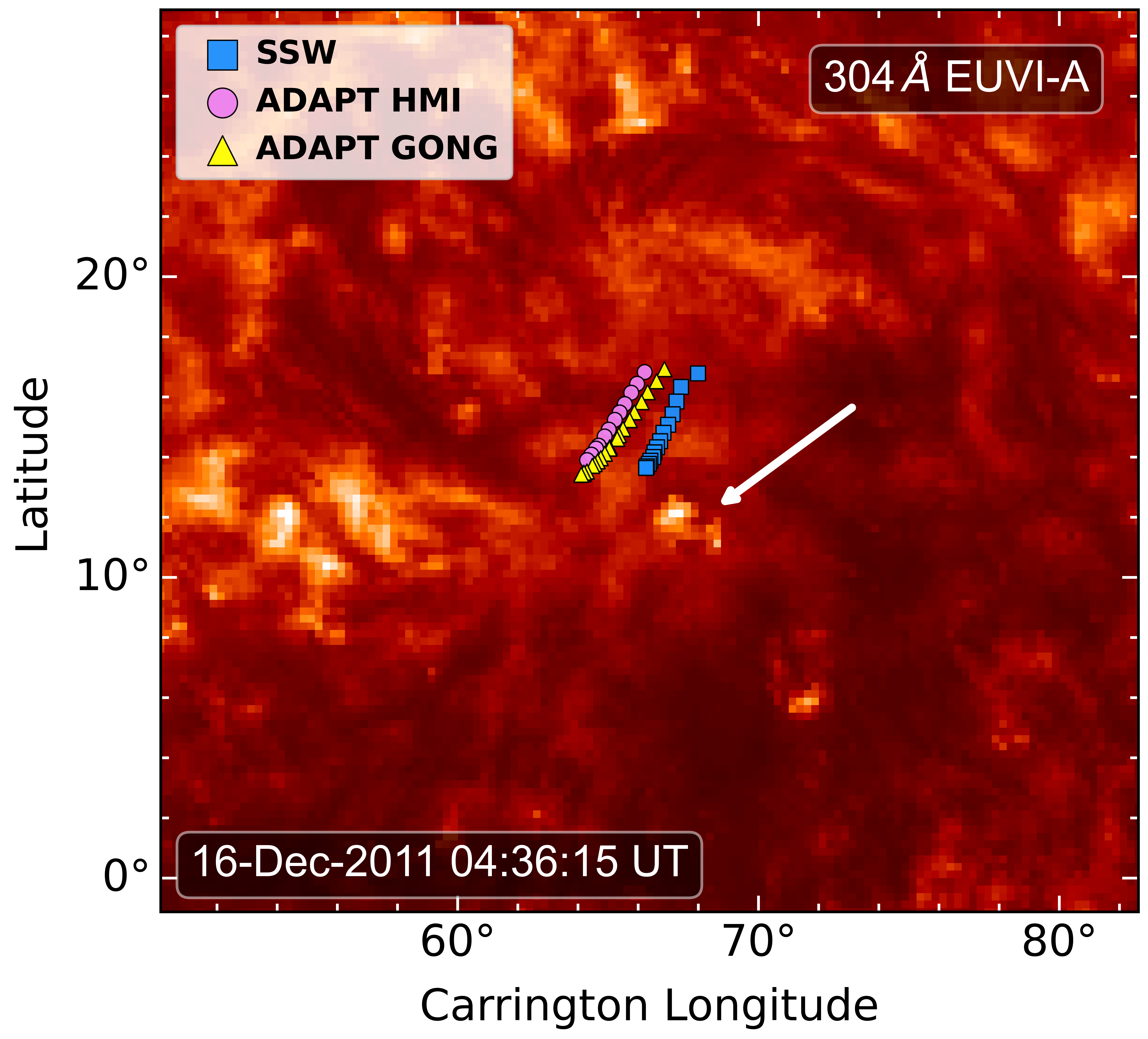
In Figure 2, we used the Bfield_20111216_000400.h5 SSW map as the photospheric boundary condition for the PFSS extrapolation. We now extend this analysis by performing PFSS extrapolations based on other synchronic magnetic maps, specifically Air Force Data Assimilative Photospheric Flux Transport (ADAPT) maps (Worden and Harvey 2000; Hickmann et al. 2015; Arge et al. 2010), using both HMI and Global Oscillation Network Group (GONG; Harvey et al. 1996) input magnetograms. Figure 6 compares the resulting connectivity footpoints for the SSW (blue squares), ADAPT HMI (pink dots), and ADAPT GONG (yellow squares) maps on December 16, 2011. The strong agreement among all three cases indicates that the inferred magnetic connectivity is not sensitive to the choice of synchronic map, demonstrating the robustness of our results.
C.2 Input PFSS parameters

We now evaluate the effect of using different input parameters on the PFSS extrapolations to test the robustness of the inferred footpoint locations and comet connectivity. In Figure 7, we compare the footpoint locations for different values of (left), (middle), and SSW synchronic map dates (right). We use SSW maps as we have seen in Figure 6 that the choice of map source does not make a significant difference in our results. In the left panel, the footpoint locations are consistent with each other, except for the coarser angular resolution with . Note that is the highest possible value based on the resolution of the input SSW synchronic map. In the middle panel, the value does not affect the connectivity.
In the right panel, we test different SSW synchronic magnetic map dates because the SFT model used to generate them assimilates observational data only within from the central meridian (Barnes et al. 2023). On December 16, the brightening site was located at 101∘ from the central meridian, meaning that the magnetic flux at this location was estimated by the model rather than directly constrained by observations. To assess whether this introduces additional uncertainties, we also use a synchronic map from a time when the brightening location lies within the assimilation window, around December 12. Although the date of the input synchronic map differs from the time of the brightening, each field line footpoint is reprojected at the correct Carrington coordinates during the brightening. We see a good agreement for the footpoint locations between the different input synchronic maps, meaning that the magnetic flux around the brightening region does not evolve a lot between December 12 and 16 and the model uncertainties remain small. These results confirm the robustness of the magnetic connectivity used throughout this paper.