Stochastic Convergence Analysis for Large-Scale Linear Discrete Ill-posed Problems
Abstract
We study weighted Tikhonov regularization for large-scale linear discrete ill-posed problems with random noise. Under a polynomial upper-bound assumption on the generalized eigenvalues of the discrete forward operator, we derive stochastic error bounds for two noise models: expectation bounds for independent zero-mean bounded-variance noise, and high-probability bounds for independent sub-Gaussian noise. The analysis yields an a priori parameter-choice rule and suggests an adaptive strategy suitable for large-scale computation. Numerical experiments support the theory and show that the predicted parameter is nearly optimal and that the adaptive method is effective in practice.
Keywords: Inverse problems, linear discrete ill-posed problems, regularization method, stochastic error estimates, optimal regularization parameter.
1 Introduction
Inverse problems play an important role in many areas of science and engineering, such as astronomy, geoscience, biomedical imaging, mining engineering, and medical diagnostics; see, for example, [1, 3, 4, 6, 8, 12, 15, 18, 17, 22, 26]. A fundamental objective in the study of inverse problems is to recover physically meaningful information from indirect measurements, which are typically contaminated by noise and other sources of uncertainty. In this paper, we consider a broad class of inverse problems that, after discretization, can be formulated as large-scale linear systems of the form
| (1.1) |
where denotes the unknown parameter vector or quantity of interest, represents the observed data, and is the discretized forward operator associated with the underlying physical or measurement process. The perturbation term accounts for measurement noise, model errors, discretization effects, and finite-precision inaccuracies. In many applications, the matrix is ill-conditioned and the data are contaminated by noise, rendering direct inversion highly unstable. As a result, the discretized system is typically a linear discrete ill-posed problem, and this has motivated a substantial body of work on regularization methods and parameter-choice strategies. Classical contributions in this direction include generalized cross-validation and the L-curve criterion; see, for example, [14, 16, 19].
Regularization is therefore indispensable for computing meaningful approximations. Among the available approaches, Tikhonov-type methods remain central because they offer a robust balance between data fidelity and stability and admit a transparent spectral interpretation. In this work we consider the weighted least-squares formulation
| (1.2) |
where is the regularization parameter, is a symmetric positive-definite weight matrix, and . This formulation includes classical Tikhonov regularization as the special case , while also allowing weighted penalties that incorporate prior structural information on the unknown. The practical success of this method depends crucially on the choice of the parameter , which must balance data fidelity against stability. If is chosen too small, the reconstruction is dominated by noise; if it is too large, important features of the exact solution are oversmoothed.
The computational difficulty becomes more pronounced in large-scale inverse problems, where fine discretizations or high-dimensional measurements make direct factorizations and full spectral decompositions impractical. In this regime, iterative regularization and hybrid projection methods have become fundamental tools. Representative contributions include hybrid LSMR for large-scale Tikhonov regularization, generalized hybrid methods for Bayesian inverse problems, recycling-based hybrid projection methods, and the recent survey on hybrid projection methods for large-scale inverse problems [10, 11, 23, 9].
Recent work has broadened this picture in several directions. On the algorithmic side, projected and iterated Tikhonov schemes with adaptive parameter choice have been developed for large-scale problems, together with refined convergence analyses for Arnoldi–Tikhonov-type methods [5, 2]. On the stochastic side, early stopping rules for stochastic mirror descent methods have been analyzed for ill-posed inverse problems [21]. At the same time, data-driven inversion has renewed attention to regularization methods that remain convergent in the classical sense [20]. These developments highlight the need for analyses that explicitly connect stochastic noise models, spectral decay, and computationally feasible regularization strategies.
Despite recent progress, stochastic convergence results for large-scale linear discrete ill-posed problems that simultaneously capture the effects of the problem size, noise strength, regularization parameter, and spectral decay remain relatively limited. This issue is particularly relevant when the data perturbation is random and one seeks estimates that are informative both theoretically and computationally, and that can also guide parameter selection.
In this paper, we investigate a Tikhonov-type regularization method for large-scale linear inverse problems with random noise. Our analysis is carried out under the following polynomial upper-bound assumption on the generalized eigenvalues associated with the discrete forward operator.
Assumption 1.1
The eigenvalues of the generalized eigenvalue problem
| (1.3) |
satisfy
for some constant .
We consider two noise models:
(M1) are independent random variables satisfying and ;
(M2) are independent sub-Gaussian random variables with parameter .
To facilitate a consistent comparison across different discretization levels and to reduce scaling effects induced by the discretization of the forward operator, we use the normalized Euclidean norm . Throughout the paper, denotes a generic positive constant whose value may change from line to line.
The main contributions of this paper are as follows. First, under the bounded-variance noise model (M1), we establish expectation-based stochastic convergence estimates for Tikhonov-regularized solutions, with explicit dependence on the noise level, the regularization parameter, and the spectral decay of the forward operator. Second, under the sub-Gaussian noise model (M2), we derive stronger high-probability bounds by combining concentration arguments with covering entropy estimates. Third, these results yield an a priori parameter-choice rule and further motivate an adaptive parameter-selection algorithm that is computationally feasible for large-scale problems. Finally, we validate the theory by numerical experiments on representative linear inverse problems, demonstrating both the near-optimality of the predicted parameter choice and the practical effectiveness of the proposed adaptive method.
The remainder of this paper is organized as follows. In Section 2, we study the case of independent noise with bounded variance and derive expectation-based stochastic convergence estimates for the weighted Tikhonov regularized solutions. Section 3 is devoted to the sub-Gaussian noise setting, where we combine concentration arguments with covering entropy estimates to establish sharper high-probability error bounds and the corresponding a priori parameter-choice rule. In Section 4, motivated by the theoretical analysis, we introduce a data-driven adaptive procedure for selecting the regularization parameter in large-scale problems. Finally, Section 5 presents numerical experiments, illustrating the near-optimality of the predicted parameter choice and the practical effectiveness of the proposed adaptive method.
2 Stochastic convergence for noisy data of variables with bounded variance
In this section, we consider the bounded-variance noise model (M1) and derive expectation-based stochastic convergence estimates for the error.
Lemma 2.1
Let be the eigenvalues of the generalized eigenvalue problem
Then the corresponding eigenvectors form an orthonormal basis of under the inner product , and satisfy .
Proof.
The eigenvalue problem (1.3) is equivalent to the generalized matrix eigenvalue problem
Define The matrix is symmetric and positive semidefinite. Hence, there exist real eigenvalues and an orthonormal basis of such that
Define , Then satisfies
and hence is an eigenvector of the generalized eigenvalue problem (1.3). Let and be eigenvectors corresponding to eigenvalues and , respectively. Then for any ,
Therefore, the eigenvectors form an orthonormal basis of under the inner product . Moreover,
Theorem 2.1
Proof. By the first-order optimality condition for the quadratic minimization problem (1.2), the unique minimizer satisfies
| (2.3) |
For , define the energy norm
Taking in (2.3), and using (1.1), we obtain
| (2.4) |
Let be the eigenvalues of
| (2.5) |
and let be the corresponding eigenvectors. By Lemma 2.1,
Hence, for any , we may write
Using the Cauchy–Schwarz inequality, we get
Therefore,
Taking expectations and using the independence, zero mean, and variance bound , we obtain
where we also used .
Finally, squaring (2.4), taking expectations, and using (2.6), we arrive at
Since
the estimates (2.1)–(2.2) follow immediately after dividing by .
Theorem 2.1 yields convergence in expectation for the output error , but only boundedness in expectation for the source error in the -norm. We next show that the source error is convergent in expectation in a weaker topology.
Lemma 2.2
3 Stochastic convergence for noisy data being sub-gaussian random variables
In this section, we turn to the case (M2) for the data model (1.1), namely,
| (3.1) |
Under this assumption, we study the stochastic convergence behavior of the errors and .
To facilitate the subsequent analysis, we first recall several basic notions and auxiliary results from the theory of sub-Gaussian random variables and empirical processes; see [7, 24, 25] for further details and general background. A fundamental feature of a sub-Gaussian random variable is that its tail decays exponentially fast. More precisely, if is sub-Gaussian, then its distribution satisfies
| (3.2) |
This tail bound plays a central role in deriving concentration inequalities for the stochastic quantities appearing in our analysis.
We shall also make use of Orlicz norms. Let be a nondecreasing convex function satisfying . Then the Orlicz norm of a random variable is defined by
| (3.3) |
In particular, throughout most of the analysis we work with the -Orlicz norm, corresponding to the function for . This norm provides a convenient way to quantify sub-Gaussian behavior. In particular, one has the estimate (see, for example, [7, (4.5)])
| (3.4) |
Next, let be a semi-metric space endowed with a semi-metric , and let be a stochastic process indexed by . The process is said to be sub-Gaussian if its increments satisfy
| (3.5) |
This increment condition is the natural analogue of sub-Gaussianity for stochastic processes and is particularly useful in conjunction with entropy estimates.
For a semi-metric space and , the covering number is defined as the minimal number of -balls required to cover . Its logarithm, , is called the covering entropy. This quantity serves as a standard measure of the complexity of the index set and will enter our estimates through a maximal inequality for sub-Gaussian processes.
More precisely, we shall use the following result from [25, Section 2.2.1].
Lemma 3.1
If is a separable sub-Gaussian random process, then there exists a constant such that
In addition, we shall also use the following two auxiliary results from [7].
Lemma 3.2
The family of random variables forms a sub-Gaussian process with respect to
Proof. For , set . Then
By independence and the sub-Gaussian assumption, for every ,
Hence
Thus is sub-Gaussian with variance proxy , which gives the asserted semi-distance
Lemma 3.3
Let and be constants, and let be a random variable satisfying
Then there exists a constant , depending only on and , such that
Lemma 3.4
Let Assumption 1.1 hold, and define Then there exists a constant , independent of , such that
| (3.6) |
for all sufficiently small .
Proof. Let be a -orthonormal family of eigenvectors associated with the generalized eigenvalue problem
so that
Then every admits the expansion and and hence
Moreover, by Lemma 2.1,
Therefore, for each with , the vectors form an orthonormal system in with respect to the Euclidean inner product. Consequently,
Denoting , the set can be represented as the ellipsoid
Now let be the constant in Assumption 1.1, so that
Define
Since , we have the inclusion
and therefore
Thus it suffices to estimate the covering number of .
Fix sufficiently small, and choose such that with the convention if . Let denote the orthogonal projection onto . For any we have
Hence
Thus every point of lies within distance of the truncated ellipsoid , and therefore
The set is the -dimensional ellipsoid with semi-axis lengths . By a standard volume comparison argument,
Taking , we obtain
Since for , it follows that and hence
Using and , we find so that
By Stirling’s formula,
and therefore
Consequently,
Finally, from we obtain which implies
Combining the above estimates yields
This completes the proof.
Theorem 3.1
Let and let be the solution of (1.2). If then there exists a constant , independent of , such that
Proof. By (3.4), it suffices to prove
| (3.7) |
Since the two estimates can be derived in the same manner, we prove only the first one by a peeling argument.
Let and be constants to be specified later, and define, for ,
| (3.10) |
Choose For , set
Then
| (3.11) |
We next estimate . For , define
Since and , we have
By Lemma 3.2, the process is sub-Gaussian with respect to For any , by the definition of ,
Therefore
Consequently,
| (3.12) |
Using Lemma 3.1, (3.12), and the definition of , we obtain
| (3.13) |
Since
we have
Therefore, by Lemma 3.4,
where the factor has been absorbed into the generic constant .
We now estimate . Suppose first that . On the event , (3.8) and (3.9) imply
Hence, by (3.14) and the -tail estimate (3.4),
| (3.15) |
For , choose
Then, under the condition
a direct computation shows that for ,
| (3.16) |
To simplify this bound, we apply Young’s inequality in the form
which gives
Substituting this into (3.16), we arrive at
The case , , is treated in the same way and gives
Combining these bounds over all , and using the facts that for ,
we obtain
Thus, by (3.11),
| (3.17) |
It then follows from Lemma 3.3 that
which is the first estimate in (3.7).
The -norm estimate is obtained by the same peeling argument, now taking and , which gives
and therefore
Using the operator introduced in Lemma 2.2, we can further derive a high-probability estimate in the corresponding weak topology.
Remark 3.1
The above results suggest the a priori parameter choice
| (3.18) |
Under this choice, one obtains the high-probability bounds
| (3.19) | ||||
| (3.20) |
4 Adaptive method to find the optimal regularization parameter
In practical applications, neither the exact solution nor, in some cases, the noise strength is available. Consequently, the a priori parameter-choice rule (2.9) is generally not directly implementable. We also note that (2.9) may be regarded as a practical approximation to the prior parameter-choice rule (3.18) in Section 3, since the two differ only by the additive term in the denominator, which is typically negligible when is large. Therefore, the two choices are asymptotically close. Motivated by this observation, we approximate the unknown solution norm by , and estimate the noise strength by the empirical residual . This leads to the following adaptive procedure for selecting the regularization parameter using only the observed data.
The proposed scheme is entirely data-driven and can be implemented in a straightforward manner. It starts from an explicit initial guess and then refines the parameter through a fixed-point type iteration until convergence. Since each update depends only on the current residual and the norm of the current regularized solution, the method is well suited for practical inverse problems in which the underlying noise characteristics are unavailable or difficult to estimate reliably.
5 Numerical results
In this section, we present several numerical experiments to complement the preceding theoretical analysis. Our main objective is to examine whether the observed numerical behavior is consistent with the theoretical predictions, including the near-optimality of the a priori parameter choice, the boundedness suggested by the error estimates, and the effectiveness of the adaptive parameter-selection algorithm. The noisy data are generated by
where consists of independent standard Gaussian random variables and
with denoting the prescribed relative noise level and representing the corresponding noise strength.
Example 5.1 (A prototypical linear inverse problem)
We consider a prototypical linear inverse problem induced by a continuous kernel , . The associated integral operator is defined by
| (5.1) |
Since the kernel is continuous on the compact set , the operator is compact on . Its adjoint operator is given by
To obtain a finite-dimensional approximation, we partition the interval into uniform subintervals and apply a quadrature rule to discretize the integral equation. This yields the linear system
where
In the present example, we choose the kernel function and the exact solution as
| (5.2) |
and respectively, and set the weight matrix to . It is well known that the kernel (5.2) is the Green’s function of the one-dimensional Dirichlet Laplacian on . Hence, the associated operator has singular values satisfying . Therefore, for a standard discretization of , the generalized eigenvalues of (1.3) behave like the squared singular values of , so that It is natural to take in Assumption (1.1) for this example.
-
•
Near-optimality of the a priori parameter choice (3.18) in terms of the output error .
With the noise level fixed at , we choose ten logarithmically equispaced values of in the interval . For each , we compute the regularized solution and evaluate the corresponding output error These values are then compared with the parameter predicted by rule (3.18), denoted by , where the implicit constant in the term is set equal to one. The same experiment is repeated for several discretization levels in order to assess whether the proposed parameter choice remains effective across different problem sizes. As shown in Figure 1, the parameter predicted by rule (3.18) is nearly optimal, in the sense that it lies close to the minimizer of the output error.


|
To examine the scaling predicted by the expectation bounds, we performed a Monte Carlo experiment for the discretization levels and the noise levels For each pair , the regularization parameter was chosen according to the predicted rule (3.18), where the implicit constant in the term is set equal to one. The corresponding regularized solution was then computed, and the expectations and with were approximated by sample averages over 2000 independent Gaussian noise realizations. The empirical means were then plotted against on log–log scales and fitted by least squares in logarithmic coordinates. As shown in Figure 2, the fitted slopes are and , respectively, which are in excellent agreement with the predicted exponents and . This provides numerical evidence for the bounds (2.10) and (2.11).
 |

|
-
•
Numerical verification of the effectiveness of Algorithm 1.
We consider the noise levels and the discretization sizes . Throughout the experiments, the stopping tolerance is set to , and Algorithm 1 is employed to determine the regularization parameter. For each pair , we report the final regularization parameter, the number of iterations, the relative reconstruction error the relative error with respect to the exact data and the relative residual with respect to the noisy data
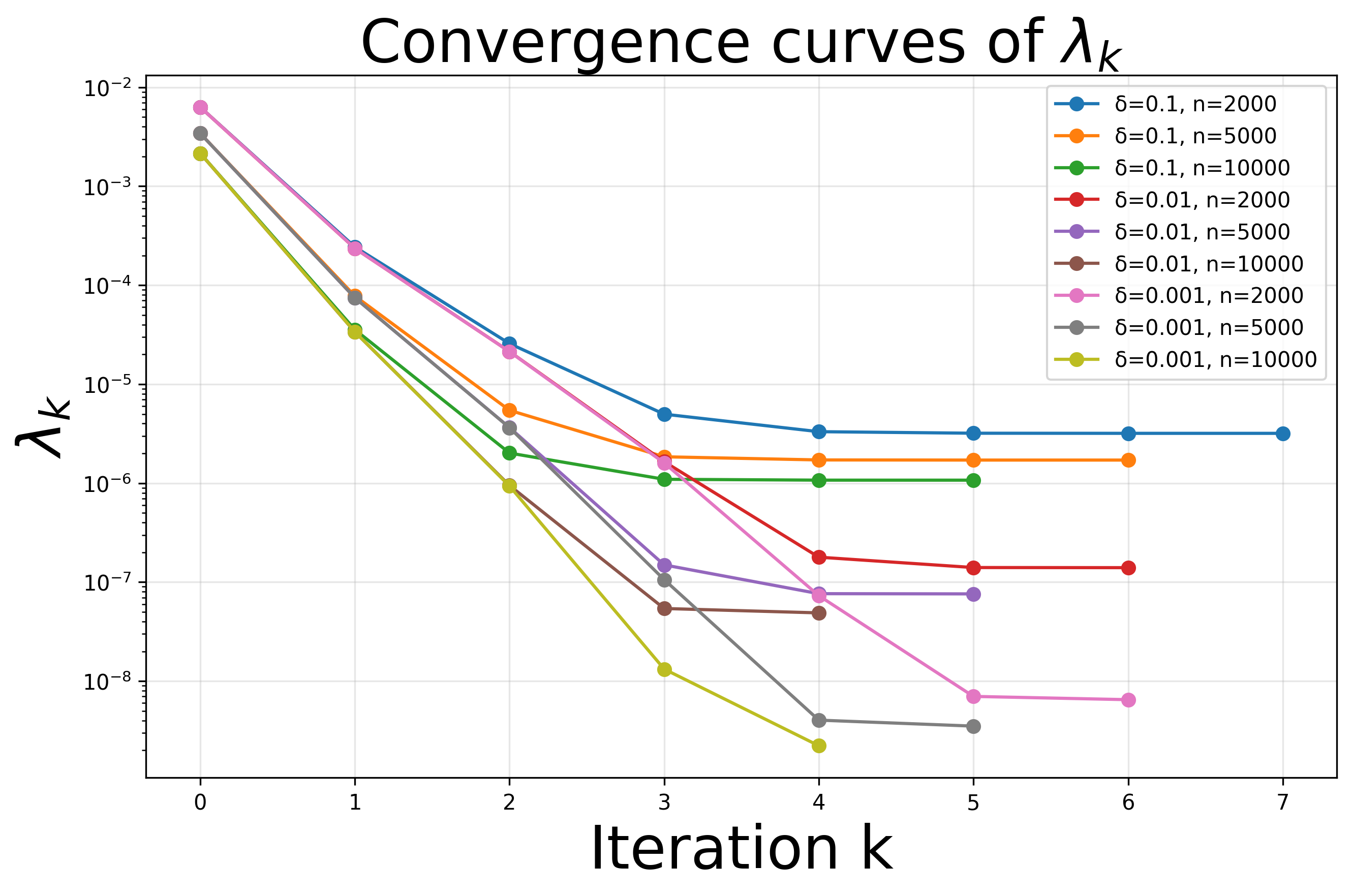
Table 1 summarizes the numerical results for all tested noise levels and discretization sizes. For each , it lists the noise strength , the final regularization parameter , the number of iterations, the relative reconstruction error, and the relative data errors with respect to both the exact data and the noisy data . The results show that decreases as the noise level decreases or the discretization size increases. Meanwhile, both the relative reconstruction error and the relative exact-data error become smaller for lower noise levels and finer discretizations, whereas the residual remains of the same order as the prescribed noise level . These results indicate that the proposed parameter-choice algorithm 1 produces stable regularization parameters and accurate reconstructions across all tested regimes.
Figure 3 shows the convergence histories of the iterative sequence . In all cases, decreases rapidly during the first few iterations and then stabilizes, which demonstrates the fast and stable convergence of the parameter-selection procedure. Figure 4 compares the reconstructed solutions with the exact solution. It can be seen that the regularized solutions remain close to the exact solution for all tested values of , and that the reconstruction accuracy improves as the noise level decreases and the discretization size increases.
| iters | |||||||
|---|---|---|---|---|---|---|---|
| 0.1 | 2000 | 8 | |||||
| 0.1 | 5000 | 7 | |||||
| 0.1 | 10000 | 6 | |||||
| 0.01 | 2000 | 7 | |||||
| 0.01 | 5000 | 6 | |||||
| 0.01 | 10000 | 5 | |||||
| 0.001 | 2000 | 7 | |||||
| 0.001 | 5000 | 6 | |||||
| 0.001 | 10000 | 5 |
 |


|
Example 5.2
This example is based on the IR Tools package [13]. We consider the blurring of the Hubble space telescope image included in the package at two resolutions, namely and pixels. These correspond to problem sizes and , respectively. Zero boundary conditions are imposed, which are natural here because the image is set against a black background.
-
•
Numerical validation of the spectral decay assumption and estimation of .
To examine the spectral decay assumption, we consider the speckle deblurring problem generated by PRblurspeckle at the two image resolutions introduced above. Since the blurring matrix generated by IR Tools is a psfMatrix object, we convert it into an explicit matrix , take , and compute the positive generalized eigenvalues of . Ordering decreasingly, we estimate the decay exponent from the log-log fit over the intermediate range , where is the number of retained positive eigenvalues. The resulting , together with the envelope , where , is then used to assess the plausibility of the algebraic decay condition . Figure 5 shows the decay of the generalized eigenvalues for two discretization levels, and , with corresponding fitted exponents and , respectively.


-
•
Near-optimality of the a priori parameter choice (3.18) in terms of the output error.
As in Example 5.1, the experiment is carried out by computing the regularized solutions over a prescribed parameter grid and comparing the resulting output errors with the theoretically predicted parameter. The figure 6 shows the same overall behavior of the output error with respect to the regularization parameter . In both cases, the error decreases as increases from very small values, attains its minimum in an intermediate range, and then rises rapidly for larger . The parameter predicted by the a priori choice rule (3.18), with the implicit constant in the term fixed at , is indicated by the red star and is seen to lie close to the minimum region of the error curve.


-
•
Empirical distribution of the output error
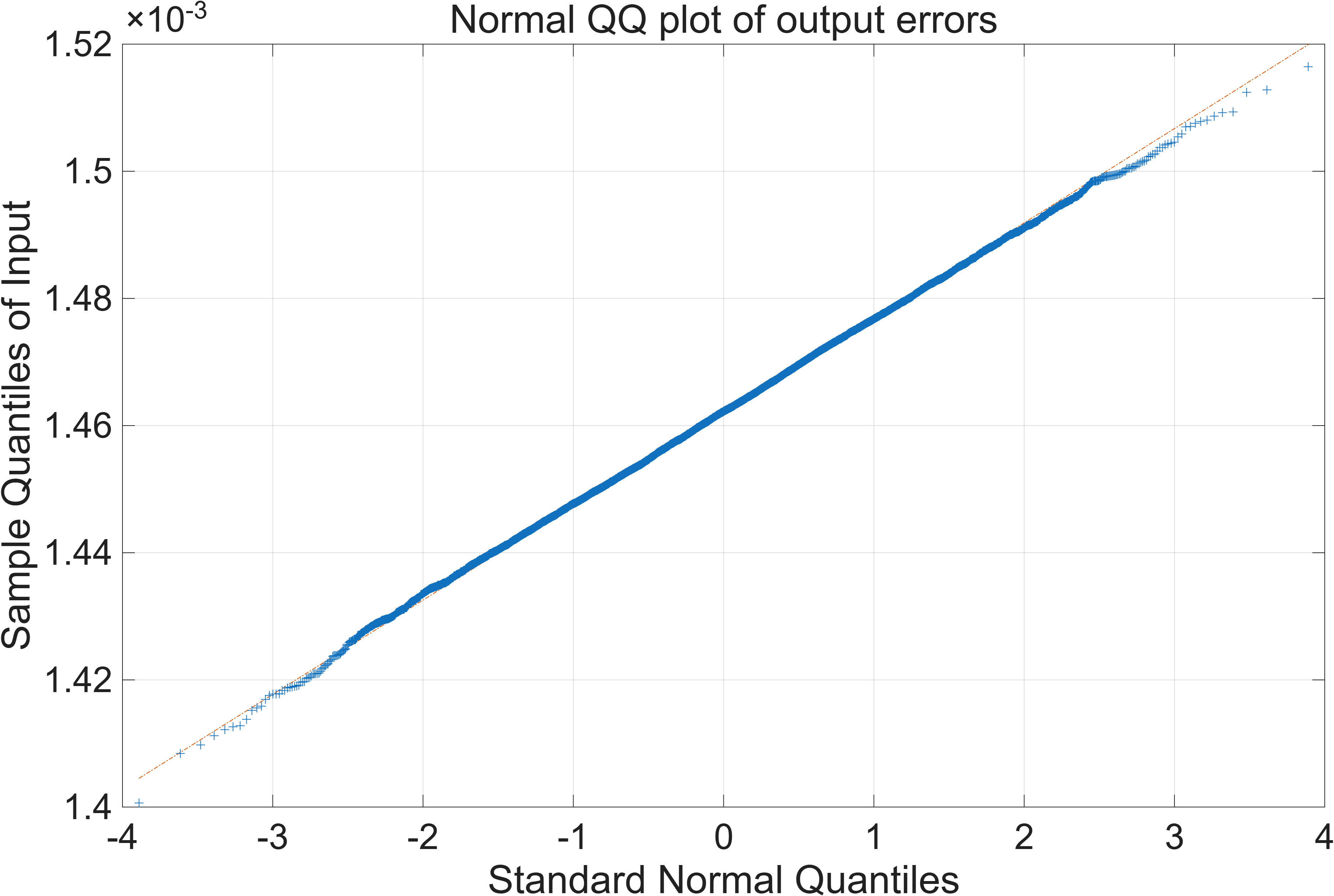
To examine the statistical behavior of the output error, we conduct a Monte Carlo experiment with and , using the parameter rule (3.18) to determine a nearly optimal . We generate independent noise realizations and record the empirical errors The histogram in Figure 7 shows a strong concentration of the errors, while the Q-Q plot is close to linear except for slight tail deviations. This indicates that the empirical distribution of the output error is well approximated by a Gaussian law and exhibits an approximately exponential, more precisely sub-Gaussian, tail decay. These observations provide qualitative support for the concentration estimate (3.19).

-
•
Performance of the adaptive parameter-choice rule
As in Example 5.1, we apply the adaptive parameter-choice Algorithm 1 to the cases , , and , ; see Figures (8(a))–(8(f)). In the implementation, the iteration is terminated when the relative change in the parameter satisfies
For and , the parameter sequence decreases quickly and stabilizes at about , while the output error decreases rapidly in the first few iterations and then levels off. For the smaller noise level with , the iteration selects a substantially smaller parameter, approximately , and achieves a lower final output error. Figures (8(e))–(8(f)) show that the adaptive method stably recovers the principal image features in both cases, while the lower noise level yields a smaller selected regularization parameter and a visibly sharper reconstruction. These results support the stability and effectiveness of the proposed adaptive procedure.


References
- [1] H. Andrews and B. Hunt. Digital Image Restoration. Prentice Hall, Englewood Cliffs, NJ, 1977.
- [2] D. Bianchi, M. Donatelli, D. Furchí, and L. Reichel. Convergence analysis and parameter estimation for the iterated arnoldi–tikhonov method. Numerische Mathematik, 157:749–779, 2025.
- [3] A. F. Boden, D. C. Redding, R. J. Hanisch, and J. Mo. Massively parallel spatially-variant maximum likelihood restoration of hubble space telescope imagery. Journal of the Optical Society of America A, 13:1537–1545, 1996.
- [4] N. K. Bose and K. J. Boo. High-resolution image reconstruction with multisensors. International Journal of Imaging Systems and Technology, 9:294–304, 1998.
- [5] A. Buccini, S. Gazzola, L. Onisk, M. Pasha, and L. Reichel. Projected iterated tikhonov in general form with adaptive choice of the regularization parameter. Numerical Algorithms, 100:1617–1637, 2025.
- [6] T. M. Buzug. Computed Tomography. Springer, Berlin, 2008.
- [7] Z. Chen, R. Tuo, and W. Zhang. Stochastic convergence of a nonconforming finite element method for the thin plate spline smoother for observational data. SIAM Journal on Numerical Analysis, 56:635–659, 2018.
- [8] J. Chung, E. Haber, and J. Nagy. Numerical methods for coupled super-resolution. Inverse Problems, 22:1261–1272, 2006.
- [9] J. Chung and S. Gazzola. Computational methods for large-scale inverse problems: A survey on hybrid projection methods. SIAM Review, 66(2):205–284, 2024.
- [10] J. Chung and K. Palmer. A hybrid LSMR algorithm for large-scale tikhonov regularization. SIAM Journal on Scientific Computing, 37(5):S562–S580, 2015.
- [11] J. Chung and A. K. Saibaba. Generalized hybrid iterative methods for large-scale bayesian inverse problems. SIAM Journal on Scientific Computing, 39(5):S24–S46, 2017.
- [12] C. L. Epstein. Introduction to the Mathematics of Medical Imaging. SIAM, Philadelphia, 2nd edition, 2007.
- [13] S. Gazzola, P. C.Hansen, and J. G. Nagy. IR Tools: A MATLAB package of iterative regularization methods and large-scale test problems. Numerical Algorithms, 81:773–811, 2019. Software available at https://github.com/jnagy1/IRtools.
- [14] G. H. Golub, M. Heath, and G. Wahba. Generalized cross-validation as a method for choosing a good ridge parameter. Technometrics, 21(2):215–223, 1979.
- [15] E. Haber. Computational Methods in Geophysical Electromagnetics. SIAM, Philadelphia, 2014.
- [16] P. C. Hansen. Analysis of discrete ill-posed problems by means of the L-curve. SIAM Review, 34:561–580, 1992.
- [17] P. C. Hansen and J. S. Jørgensen. AIR tools II: Algebraic iterative reconstruction methods, improved implementation. Numerical algorithms, 79:107–137, 2018. Software available at https://github.com/jakobsj/AIRToolsII/.
- [18] P. C. Hansen, J. G. Nagy, and D. P. O’Leary. Deblurring Images: Matrices, Spectra, and Filtering. SIAM, Philadelphia, PA, 2006.
- [19] P. C. Hansen and D. P. O’Leary. The use of the L-curve in the regularization of discrete ill-posed problems. SIAM Journal on Scientific Computing, 14(6):1487–1503, 1993.
- [20] A. Hauptmann, S. Mukherjee, C.-B. Schönlieb, and F. Sherry. Convergent regularization in inverse problems and linear plug-and-play denoisers. Foundations of Computational Mathematics, 25:1087–1120, 2025.
- [21] J. Huang, Q. Jin, X. Lu, and L. Zhang. On early stopping of stochastic mirror descent method for ill-posed inverse problems. Numerische Mathematik, 157:539–571, 2025.
- [22] S. M. Jefferies, K. J. Schulze, C. L. Matson, K. Stoltenberg, and E. K. Hege. Blind deconvolution in optical diffusion tomography. Optics express, 10:46–53, 2002.
- [23] J. Jiang, J. Chung, and E. de Sturler. Hybrid projection methods with recycling for inverse problems. SIAM Journal on Scientific Computing, 43(5):S146–S172, 2021.
- [24] S. A. van de Geer. Empirical Processes in M-Estimation. Cambridge University Press, Cambridge, 2000.
- [25] A. W. van der Vaart and J. A. Wellner. Weak Convergence and Empirical Processes. Springer, New York, 1996.
- [26] Y. Wang. Regularization for inverse models in remote sensing. Progress in physical geography, 36:38–59, 2012.