Numerical methods for optimal decumulation of a defined contribution pension plan
Abstract
The decumulation of a defined contribution (DC) pension plan is well known to be one of the hardest problems in finance. We model this decumulation challenge as an optimal stochastic control problem. The control problem is solved, at each rebalancing date, by alternatively solving a linear partial-integro differential equation (PIDE) followed by an optimization step. We solve the PIDE by using a -monotone Fourier method, which ensures that monotonicity holds to . We allow for the use of leverage (i.e. borrowing to invest in stocks), as well as minimum constraints on bond holdings. We pay particular attention to minimizing wrap-around error, an issue which is endemic for Fourier methods and central to the effective use of these methods for optimal control problems. Rather unexpectedly, we find that restricting the portfolio equity fraction to a maximum of 50% does not reduce portfolio efficiency noticeably. This may be a useful strategy for risk-averse retirees.
Keywords: decumulation, stochastic control, risk
JEL codes: G11, G22
AMS codes: 91G, 65N06, 65N12, 35Q93
1 Introduction
In developed countries, there is a strong and growing shift from Defined Benefit (DB) pension plans to Defined Contribution (DC) plans. The private sector, and increasingly government institutions, are unwilling to take on the balance sheet liabilities of a DB plan (Thinking Ahead Institute, 2024).
Under a DC plan, the employer and employee contribute to a (usually) tax advantaged account, which is typically invested in a mix of stocks and bonds. Upon retirement, the employee is now responsible for both choosing an investment strategy and deciding on a withdrawal schedule. Although it is often advocated that retirees should buy annuities, these are unpopular with DC plan holders (Peijnenburg et al., 2016) for numerous valid reasons (MacDonald et al., 2013). In particular, annuities are generally overpriced, lack true inflation protection and retirees have no access to capital in the event of emergencies.
Since it is usually challenging to fund a reasonable lifestyle investing solely in riskless assets, the retiree is now exposed to both investment risk and longevity risk. This problem of funding retirement from accumulated DC capital, also known as the decumulation problem, has been termed “the nastiest, hardest problem in finance,” by Nobel Laureate William Sharpe ( quoted in (Ritholz, 2017) ).
There have been several suggestions for DC plan spending rules (Anarkulova et al., 2025). Probably the most ubiquitous rule is the four per cent rule (Bengen, 1994). This rule suggests that retirees can withdraw four per cent of their initial capital (at age 65) annually, adjusted for inflation. Based on historical US data, an investor who invested in a portfolio of 50% bonds and 50% stocks (rebalanced annually), and followed the four per cent rule, would have never run out of savings over any thirty year historical period.
However, the four per cent rule has many critics. For example, rolling thirty year periods have high correlations. In addition, a fixed withdrawal schedule, as well as a constant weight stock allocation is somewhat simplistic. In order to better stress test spending rules, Anarkulova et al. (2025) use block bootstrap resampling of historical data, to generate a distribution of outcomes. We will also use block bootstrap resampling to test our results in this chapter.
Decumulation strategies are naturally posed as a problem in optimal stochastic control. The controls in this case are the stock/bond split on each rebalancing date and the (real) annual withdrawal amounts. In our case we impose maximum and minimum constraints on the withdrawal amounts and also impose constraints on the maximum stock allocation.
1.1 Our Contributions
In this chapter, we consider the same scenario posed in Bengen (1994). Our objective function is to maximize total withdrawals over a thirty year period (with minimum/maximum annual constraints) and minimize the risk of running out of savings before year thirty.
An optimal stochastic control problem used for decumulation is solved at each rebalancing date, by alternatively solving a linear partial-integro differential equation (PIDE) followed by an optimization step. The PIDE is solved by using a -monotone Fourier method, which ensures that monotonicity holds to , an important property for control problems. The monotone technique generalizes the method described in Forsyth and Labahn (2019). Our basic dynamic programming technique is similar to the high-level description in Forsyth (2022), but here we delve much deeper in describing the numerical methods. In particular, we focus on such issues as wrap-around errors in Fourier methods for Partial-Integro Differential Equations (PIDEs), and the 2-d -monotone Green’s function approximation.
Previous studies for decumulation have imposed no-shorting and no-leverage constraints on stock investments. In this chapter, we relax the no-leverage constraint on the stock investment and also investigate more restrictive investments in stocks. For example, a risk averse retiree may wish to restrict the maximum fraction invested in equities to be significantly less than one.
Rather surprisingly, we find that restricting the maximum fraction in stocks to be 50% does not lower the efficient frontier by a large amount. The most significant effect of the 50% restriction, compared to allowing a maximum stock fraction of up to 130% (leverage) is that the time for the median withdrawals to reach the maximum is delayed by one year. This may be an acceptable trade-off for risk averse investors.
From the numerical point of view, when solving optimal control problems using Fourier methods, wrap-around error can be significant, due to the possible instantaneous movement to domain boundaries at reallocation times (Lippa, 2013; Ignatieva et al., 2018; Alonso-Garcca et al., 2018). We show that our technique reduces wrap-around error to almost machine level precision.
1.2 Organization of this Chapter
The rest of this chapter is organized as follows. In the next section we state our problem setting followed by a mathematical formulation of our model in Section 3. The latter section includes information on the stochastic processes followed by bonds and stocks along with a description of our control set. Section 4 describes our conflicting risk and reward measures, Expected Shortfall and Expected Withdrawals, while Section 5 looks at how one maximizes these conflicting measures, something which is initially set up as a pre-commitment problem which is not implementable. Section 6 then discusses how one can formulate our problem into an (implementable) dynamic program, one which is solved by a PIDE between withdrawal time intervals. Section 7 then shows how one can solve these PIDEs using Green’s functions and Fourier analysis. The wrap-around problem that comes with using Fourier analysis and periodicity is addressed in the next section. That section also includes the resulting numerical algorithm for solving our optimal control decumulation problem. Section 9 then presents an example along with its numerical solution followed in the next section by tests of robustness of our numerical example. The paper ends with a conclusion along with an Appendix providing extra details regarding the wrap-around error discussed earlier.
2 Problem Setting
As noted in Anarkulova et al. (2025), retirees have a revealed preference for spending rules, such as that advocated by Bengen (1994). Spending rules (such as the four per cent rule) are popular with retirees as they are simple to implement, have an intuitive interpretation, and the rolling 30 year backtests in Bengen (1994) are easy to understand.
In this paper we restrict attention to the scenario outlined in Bengen (1994), that is, we consider a 65-year old retiree who desires fixed minimum annual (real) cash flows over a 30 year time horizon. We also impose an upper limit (a cap) on maximum withdrawals in any year. From the CPM2014 table from the Canadian Institute of Actuaries111www.cia-ica.ca/docs/default-source/2014/214013e.pdf., the probability that a 65-year old Canadian male attains the age of 95 is about 0.13. In spite of this relatively low probability of achieving the age of 95, assuming a 30 year time horizon is considered a prudent approach for minimizing the risk of exhausting savings. In addition, observe that we will not mortality weight future cash flows, as is done when averaging over a population for pricing annuities. Mortality weighting may not be meaningful for an individual investor, since it reflects population averages, rather than the circumstances of an individual retiree.
Since we allow investing in risky assets, with a minimum cash withdrawal each year, it is possible to exhaust savings.222Ignoring the trivial and unlikely case where investing in riskless assets can fund 30 year minimum withdrawals. In this case, we continue to withdraw funds from the portfolio, which is equivalent to borrowing cash. In such circumstances, we assume that withdrawals continue, something which can be viewed as borrowing against other resources. This debt accumulates at the borrowing rate. Essentially, we are assuming that the investor has other assets, for example real estate, which can be used as a hedge of last resort. In this case, this debt could then be funded using a reverse mortgage, with real estate as collateral (Pfeiffer et al., 2013).
It is important to note that an implicit assumption here is that real estate is not fungible with other financial assets, except as a last resort. This mental separation of assets is a common aspect of behavioral finance (Shefrin and Thaler, 1988). Real estate in this case has a dual role: if market returns are exceptionally strong, or the retiree passes away earlier than expected, this property can be a bequest. If market returns are poor, or in the case of extreme longevity, then real estate can be used to fund expenses if the retirement account is exhausted.
3 Mathematical Formulation
We assume that the investor has access to two funds: a broad market stock index fund and a constant maturity bond index fund. Let and denote the real (inflation adjusted) amounts invested in the stock index and the bond index, respectively, at time with being the investment horizon. These amounts will evolve over time, depending on the investor’s asset allocation, and changes in the real unit prices of the assets. In the absence of an investor determined control such as cash withdrawals or rebalancing, any changes in and result from asset price evolution. We model the stock index as following a jump diffusion, which permits modelling both continuous stochastic processes as well as market jumps.
We model the real returns of a constant maturity bond index as a stochastic process (see for example, Lin et al., 2015; MacMinn et al., 2014). This avoids the need to model bond prices and inflation separately. As done in MacMinn et al. (2014), we assume that the constant maturity bond index follows a jump diffusion process, with justification being found in Forsyth et al. (2022, Appendix A).
3.1 The Diffusion Processes.
For any time let
denote the values of the instant before and the instant after time . Such notation will also be used for any other time dependent function. We let be a random number representing a jump multiplier, that is, when a jump occurs, . The use of a jump process accounts for non-normal asset returns. As in (Kou, 2002; Kou and Wang, 2004), we assume that follows a double exponential distribution with the probability of an upward jump and the probability of a downward jump. The density function for is
| (1) |
We also define
| (2) |
where is the expectation. In the absence of control, evolves according to
| (3) |
where is the (uncompensated) drift rate, is the volatility, is the increment of a Wiener process, is a Poisson process with positive intensity parameter , and the are i.i.d. positive random variables having distribution (1). Moreover, , , and are assumed to all be mutually independent.
Similarly, let the amount in the bond index the instant before be . In the absence of investor intervention, evolves as
| (4) |
where the terms in equation (4) are defined analogously to equation (3). In particular, is a Poisson process with positive intensity parameter , and the density function for is
and . Again , , and are assumed to all be mutually independent. The term in equation (4) represents the extra cost of borrowing, that is, the spread.
The diffusion processes are correlated, that is, . However, contrary to common belief, an analysis of historical data suggests that the stock and bond jump processes are essentially uncorrelated (see Forsyth (2020b) for empirical justification). We make this assumption in this work.
We define the investor’s total wealth at time as
In case of insolvency, the portfolio is liquidated, trading stops and any outstanding debt accrues interest at the borrowing rate.
3.2 The Set of Controls.
Consider a set of discrete times
where we assume that is constant. Here is the inception time of the investment and is the set of withdrawal/rebalancing times, as defined in equation (3.2). At each rebalancing time , , the investor first withdraws an amount of cash from the portfolio, and then afterwards rebalances the portfolio. At the portfolio is liquidated and no cash flow occurs. This is enforced by specifying .
Let
denote the instant before withdrawals and rebalancing at , we then have that is given by
with since .
Typically, DC plan savings are held in a tax-advantaged account, with no taxes triggered by rebalancing. With infrequent (e.g. yearly) rebalancing, we also expect other transaction costs, to be small, and hence can be ignored. It is possible to include transaction costs, but at the expense of increased computational cost (Van Staden et al., 2018).
Let , denote the multi-dimensional controlled underlying process and the realized state of the system. The rebalancing control is the fraction invested in the stock index at the rebalancing date , that is,
Let be the amount withdrawn at time , that is, . Formally, the controls depend on the state of the investment portfolio, before the rebalancing occurs, that is, and , where is the set of rebalancing times. However, it will be convenient to note that in our case, we find the optimal control amongst all strategies with constant wealth (after withdrawal of cash). Hence, with some abuse of notation, we will now consider to be a function of wealth after withdrawal of cash, where we use the shorthand notation and for the variables representing wealth the instant before and instant after . Using a similar shorthand notation for and we then have
Note that the control for depends only on . Since , it follows that
which we discuss further in Section 6.
A control at time is then given by the pair where the notation denotes that the control is a function of the state. Let represent the set of admissible values of the controls . We impose no-shorting, bounded leverage constraints (assuming solvency) along with maximum and minimum values for the withdrawals. In addition we apply the constraint that in the event of insolvency due to withdrawals (), or in the case of leverage, trading ceases and debt (negative wealth) accumulates at the appropriate borrowing rate of return (that is, a spread over the bond rate). We also specify that the stock assets are liquidated at .
We can then define our controls by
| (5) | ||||
| (6) |
The rather complicated expression in equation (5) imposes the assumption that as wealth becomes small, the retiree first tries to avoid insolvency as much as possible and in the event of insolvency, withdraws only .
The set of admissible values for , can then be written as
| (7) |
For implementation purposes, we have written equation (7) in terms of the wealth after withdrawal of cash. However, we remind the reader that since , the controls are formally a function of the state before the control is applied.
The admissible control set can then be written as
with an admissible control written as
We also define as the tail of the set of controls in , that is,
and , the tail of the admissible control set, as
so that .
4 Risk and Reward
In this section we consider our measures of risk and reward for our retiree. In this case the retiree is primarily concerned with the risk of depleting savings while at the same time hoping to maximize the cash withdrawals from his plan.
4.1 Risk: Expected Shortfall (ES)
Two typical measures of financial tail risk of an investment portfolio are Value at Risk (VAR) and Conditional Value of risk (CVAR), with the latter also known as Expected Shortfall. Expected Shortfall is an alternative to value at risk that is more sensitive to the shape of the tail of the loss distribution.
Suppose
where be the probability density function of wealth at . Then can be viewed as the Value at Risk (VAR) at level since the probability of wealth being more than is . For example, if , then 99% of the outcomes have . If is sufficiently large, this suggests very low risk of running out of savings. The Expected Shortfall (ES) at level is then
| (8) |
which is the mean of the worst fraction of outcomes. Typically . The definition of ES in equation (8) uses the probability density of the final wealth distribution, not the density of loss. Hence in our case, a larger value of ES, that is, a larger value of average worst case terminal wealth, is desired. 333In practice, the negative of is often the reported VAR. and the negative of ES is commonly referred to as Conditional Value at Risk (CVAR).
Define . Given an expectation under control , , then as noted by Rockafellar and Uryasev (2000), the expected shortfall at level has the alternate formulation as
| (9) |
The admissible set for in equation (9) is over the set of possible values for .
The notation emphasizes that is as seen at , that is, the pre-commitment . A strategy based purely on optimizing the pre-commitment value of at time zero is time-inconsistent. As such it has been termed by many as non-implementable, since the investor has an incentive to deviate from the time zero pre-commitment strategy at . However we consider the pre-commitment strategy merely as a device to determine an appropriate level of in equation (9). If we fix for all positive , then this strategy is the induced time-consistent strategy (Strub et al., 2019; Forsyth, 2020a; Cui et al., 2022) and hence is implementable. For further discussion of the relationship between time consistent and pre-commitment strategies, see (Vigna, 2014; Menoncin and Vigna, 2017; Vigna, 2022; Strub et al., 2019; Forsyth, 2020a; Bjork et al., 2021; Cui et al., 2022). In particular, see Forsyth (2020a) for discussion of the induced time consistent policy resulting from the use of ES risk.
An alternative measure of risk could be based on variability of withdrawals (Forsyth et al., 2020). However, we note that we have constraints on the minimum and maximum withdrawals, so that variability is mitigated. We also assume that given these constraints, the retiree is primarily concerned with the risk of depleting savings, something which is well measured by ES.
4.2 Reward: Expected Total Withdrawals (EW)
We will use expected total withdrawals as a measure of reward in the following. More precisely, we define EW (expected withdrawals) as
| (10) |
where we assume that the investor survives for the entire decumulation period. This is consistent with the scenario in Bengen (1994) .
We remark that there is no discounting term in equation (10) as all quantities are real, that is, inflation-adjusted. It is straightforward to introduce discounting, but we view setting the real discount rate to zero to be a reasonable and conservative choice. See Forsyth (2022) for further comments.
5 Maximizing Conflicting Measures: Problem EW-ES
Expected withdrawals (EW) and expected shortfall (ES) are two conflicting measures. We handle this by using a scalarization technique to find the Pareto points for this bi-objective optimization problem, that is, the set of points where one objective cannot be improved without worsening the other. For a given scalarization parameter , the goal is to then find the control that maximizes
More precisely, we define the pre-commitment EW-ES problem problem in terms of the value function derived from (9) and (10):
| (11) | ||||
| subject to | (12) |
Note that we have added an extra term to equation (11). If we have a maximum withdrawal constraint, and if as , then the controls become ill-posed. In this fortunate state for the investor, we can break investment policy ties either by setting , which will force investments in bonds, or by setting , which will force investments into stocks. Choosing ensures that this term only has an effect if and . See Forsyth (2022) for more discussion of this.
We can interchange the 444Let , then , , s.t. . Then . Hence, implies . Similarly . in equation (11) to represent the value function as
| (13) |
Since the inner supremum in equation (13) is a continuous function of and the optimal value of in equation (13) is bounded, 555This is the same as noting that a finite value at risk exists. we can define
| (14) |
Given from equation (14), then the optimal control which solves Problem (13) is the same control which solves
| (15) |
Hence Problem (15) is the induced time consistent policy for Problem (13). We refer the reader to Forsyth (2020a) for an extensive discussion concerning pre-commitment and time consistent expected shortfall strategies.
6 Formulation as a Dynamic Program
We can use the method in Forsyth (2020a) to determine our value function. Write (13) as
where is defined as
| (16) | ||||
| subject to | (17) |
The original problem (13) has therefore been decomposed into two steps:
6.1 Dynamic Programming Solution of Problem (16)
We give a brief overview of the method described in detail in (Forsyth, 2022). We apply the dynamic programming principle to
| (19) |
If we set
| (20) |
then equation (19) becomes
| (21) |
This approach effectively replaces a two dimensional optimization for , by two sequential one dimensional optimizations. From equations (20) and (21), the optimal pair satisfies
In other words, the optimal withdrawal control is only a function of total wealth before withdrawals while the optimal control is a function only of total wealth after withdrawals. If a withdrawal results in , then the optimal control for is determined along lines of constant wealth in the plane while if a withdrawal results in , then stocks are liquidated (). This is illustrated in Figure 1.

At , we have
while at points in between rebalancing times, that is when , standard arguments from SDEs (3-4), and Forsyth (2022) give
| (22) |
It is convenient to consider the two cases and separately. For , we solve
| (23) |
When , it is convenient to re-write equation (22) in terms of debt . Letting in equation (22) we obtain
| (24) |
Note that equation (24) is now amenable to a transformation of the form since , something required when using a Fourier method (Forsyth and Labahn, 2019; Forsyth, 2022) to solve equation (24).
After rebalancing, if , then cannot become negative, since is a barrier in equation (22). However, can become negative after withdrawals, in which case remains in the state . There equation (24) applies, unless there is an injection of cash to move to a state with . The terminal condition for equation (24) is
7 The -Monotone Fourier Method
The -monotone Fourier method originated with the work of Forsyth and Labahn (2019), where it was applied to one dimensional problems in stochastic control. In the following, we give a sketch showing how to extend those methods to work for two dimensional problems.
We illustrate this method by focusing on equation (23). Since we can let with . Then (23) converts to
| (25) |
The exact solution of equation (25) can be written as
| (26) |
where is the Green’s function of equation (23) (Garroni and Menaldi, 1992).
Remark 1(Form of Green’s function)
Note that the Green’s function for equation (23) is of the form , that is a function of the differences. Intuitively, we can view the Green’s function as a scaled probability density , and this means that depends only on the difference, . See Forsyth and Labahn (2019) for more discussion of this observation.
The Fourier transform pair for the Green’s function is given as
| (27) |
where . Standard techniques then give the Fourier Transform of the Green’s function for equation (25) as
| (28) |
where
| (29) | |||||
Here are the complex conjugates of the Fourier transforms of the density functions :
7.1 Localization
Define
As is typically the case, we assume that the Green’s function decays to zero as . More precisely, we assume that
Assumption 1 (Decay of Green’s Function)
For some , is negligible if .
We choose our region so that we can assume that the Green’s function is negligible for . As such we replace the Fourier transform pair (27) by their Fourier series equivalent
| (30) |
with
along with a localized version of equation (26)
Scaling factors in equation (30) are selected to correspond to a finite domain form of equation (27).
7.2 Periodic Extension
We have informally derived the expression for the Green’s function by localizing the infinite domain Green’s function. Localizing the problem on , and using a Fourier series representation of the Green’s function makes the implicit assumption of periodic extension.
Assumption 2
Periodicity
-
1.
The control problem is defined on the finite domain .
-
2.
The solution is extended periodically
(32) -
3.
The jump size density functions are defined on and , with periodic extension
(33) - 4.
-
5.
From equation (30) we can also see that
7.3 Discretization
We discretize equation (LABEL:green_local) on a grid , by setting
| ; | ||||
Define linear basis functions as
with a similar definition for . We can then represent the solution as a linear combination of the basis functions
| (34) |
Substituting equation (34) into equation (LABEL:green_local) then gives
For a given pair the double integrals then simplify to
Here the last line follows from the property of linear basis functions,
Defining
then implies that for each the convolution (LABEL:convolve_a) can be written as
| (36) |
Furthermore using the Fourier series form for from equation (30) we have
Here for the inside integrals in (LABEL:smooth_g_1) we have used the following formula for linear basis functions
with a similar result for the integral involving . We note that on a uniform grid and , with the result that , and . Consequently, equation (LABEL:smooth_g_1) is independent of .666For the case of in equation (LABEL:smooth_g_1) we take the limiting value as .
For future reference, we note the DFT pair for any grid function777Note that the DFT here is independent of any physical coordinates. is given by
| (38) | |||||
| (39) |
which can be verified by substituting equation (38) into equation (39)
since
| (40) |
We denote this pair by .
Discrete Index Domain
Although we have defined the solution on the physical domain , note that from equation (LABEL:smooth_g_1) is independent of . In addition, the DFT pair is defined independently of the original grid. Consequently, in order to avoid confusion concerning the various physical and grid domains, we will refer only to discrete index domains. Define
Then are both in the index domain .
7.4 Efficient Computation of the Discrete Convolution
The discrete convolution (36) is performed at each rebalancing date, hence an efficient evaluation is desirable. The convolution can be written as
| (41) | |||||
Using equations (38) and (39) to write in equation (41) gives
where we have used equation (40) in the last step. More compactly we can write
| (42) |
where is the Hadamard product of vectors .
7.5 -Monotonicity
Using the definition for from equation (LABEL:smooth_g_1), then this represents an exact integration over linear basis functions of the exact Green’s function (with periodic boundary conditions) on . Hence
| (43) |
This gives rise to an important monotonicity property (Forsyth and Labahn, 2019). Suppose we have two discrete solutions such that
| (44) |
Then, using the time advance algorithm (36), it follows that the discrete comparison principle holds:
The positivity condition (43) ensures that the order property (44) is preserved by the discretized algorithm. This is, of course, a property of the exact solution. This property is important since we compare the values of the discrete solution in order to determine the optimal control. See Forsyth and Labahn (2019) for more discussion of this.
However, note that the dimension of is , but we need to sum an infinite series to determine the discrete values of from equation (36). In practice, we truncate the series in equation (LABEL:smooth_g_1), that is,
where the grid sizes can be chosen independently from . However, truncating the Fourier series means that the positivity condition (43) may not hold any longer. In Forsyth and Labahn (2019), it is suggested that be selected so that
| (46) |
This ensures that the cumulative effect (after steps) of non-positivity means that the discrete comparison principle holds to . Note that if the timestep is constant (which is usually the case), then equation (LABEL:smooth_g_trunc) needs to be computed only once. Hence it is inexpensive to select sizes which satisfy condition (46). Equation (LABEL:smooth_g_trunc) can also be computed efficiently using FFTs, assuming are powers of two (see Forsyth and Labahn (2019).
8 Periodicity and the problem of Wrap-around error
Localization of the Green’s function effectively implies a periodic extension of the Green’s function and the solution (see Assumption 2). In option pricing applications, this wrap-around error does not cause difficulty. However, in control applications, impulse controls (such as rebalancing) may require extensive use of solution values near the edges of the grid. For example, derisking by investing in an all bond portfolio results in an impulse control which drives instantaneously. This can cause significant wrap-around pollution (see (Lippa, 2013; Ruijter et al., 2013; Ignatieva et al., 2018)).
Given the localized problem defined on , with widths
we construct an auxiliary grid with nodes in the direction, and nodes in the direction, on the domain , with
Although we have increased the size of the physical domain , we remind the reader of the discussion in Section 7.3. It will be more convenient in the following to refer to the extended index domain
Denote the projected Green’s function for grid indexes in by . Note from equation (LABEL:smooth_g_1) that does not depend on the actual physical domain, but only on . We construct and store the DFT of the projection of the Green’s function on this auxiliary index grid .
Before applying the time advance algorithm (42) we form the padded array :
| (47) |
where is an asymptotic form of the solution which we assume to be available from financial reasoning. On the auxiliary grid, the points where or correspond to the points where or , with very small grid spacing. Hence extending the solution by constant values to the left and bottom is expected to generate a very small error.
We then modify the time advance algorithm (42) as shown in Algorithm 1. Note that the step (3) discards the computed solution in the padded areas , since these points may be contaminated by wrap-around errors.
8.1 Error Due to Wrap-around
Let and , with fixed. We can then write the discrete convolution (41) in the physical domain, compactly as
| (48) |
Note that the righthand side of equation (48) uses the padded values for , but generates the unpadded on the lefthand side. In addition, is periodic with period in the direction, and period in the direction.
The use of Algorithm 1 means that the periodic extension of is used in equation (48) for any terms of the sum such that
This periodic extension wraps around the solution domain. For example, points with indexes reference points with index , which is at the opposite side of the grid, and potentially generates wrap-around error. See also Appendix 13 for further discussion of this.
Definition 1(Wraparound error.)
Assume for is periodic
| (49) |
Suppose is determined by boundary data for , which we assume to be exact,888In practice, we use the method in equation (47), which we expect will generate a small error. with . Then, the wrap-around error for convolution (48) evaluated using DFTs, at timestep , denoted by is
| (50) |
We now state a theorem on the effectiveness of our padding method. See Appendix 13 for a proof.
Theorem 8.1(Wraparound error)
Suppose for is periodic as defined in equation (49), and that be determined by boundary data for , with . Assume further that there exists a constant such that
and that we choose sufficiently large so that
| (51) |
Then
| (52) |
and the wrap-around error after steps is bounded by
Remark 2(Asymptotic Form of Green’s Function)
8.2 Numerical Method for Optimal Control
As mentioned in Section 16, we need the optimal pair at each rebalancing date. The optimal controls are obtained by first discretizing the controls and thereafter determining the controls by exhaustive search. Recall that the PIDE grid spacing is . Let and denote the number of points in the discretizations of and , respectively. We will also need to discretize the possible values of total wealth , with denoting the number of discrete wealth values. This approach (discretization and search), is then guaranteed to converge to the viscosity solution of the optimal control problem in the limit as
| ; | (53) |
which is discussed in Section 8.3.
Given an array of discrete values, that is, , we denote the linear interpolant of the grid values at an arbitrary point by
8.3 Convergence to the Viscosity Solution
Convergence of a numerical method for HJB equations is ensured provided that the complete numerical scheme is monotone, consistent and stable, (see Barles and Souganidis (1991); Forsyth and Labahn (2019)). We should clarify that each of these properties must be verified for the complete numerical scheme, including the time advance and the impulse control update.
Stability is easily established using the techniques in Forsyth and Labahn (2019). The time advance step is -monotone by construction. The optimization and projection steps in equations (54-56) are monotone, since linear interpolation is used at all off grid points. Note that extrapolation is never used (which ensures stability).
Proving consistency is a bit more involved. The key is to note that consistency, in the viscosity sense, is defined in terms of smooth, infinitely differentiable test functions. This means that proof of consistency involves replacing all the functions in equations (54-56) by smooth test functions. Discretizing the control and using linear interpolation means that the maximum of the smooth test functions in equations (54-56) will converge to the global maximum in the limit.
While the discretization of the control and use of exhaustive search may appear to be crude, this technique (coupled with linear interpolation) is the only method which is guaranteed to converge to the global maximum of a (possibly) non-convex smooth test function. This is not merely a point of academic interest. Initial attempts to use standard optimization methods sometimes resulted in convergence to a different solution (compared to the solution obtained by exhaustive search). Since the viscosity solution is unique, we can deduce that the solution obtained without using exhaustive search was spurious.
However, numerical experiments show that the discretization of the control can be quite coarse, and this does not appear to impede convergence. A non-rigorous explanation of this effect is that a smooth function has a vanishing first derivative at extreme points.
8.4 Summary: Algorithm for Problem (16).
Algorithm 2 summarizes the final algorithm. The initial set-up cost is computing the Fourier weights on the extended domain . Each timestep consists of first determining the optimal control, then followed by advancing to the next rebalancing time using the precomputed weights .
Remark 3(Use of linear interpolation)
Equations (54-56) make heavy use of linear interpolation. As discussed in Forsyth and Labahn (2019)) this is the only interpolation method (in general) which will preserve -monotonicity. This means that the convergence rate cannot exceed second order in the grid spacing. This is in contrast to the methods in (Fang and Oosterlee, 2008; 2009; Ruijter et al., 2013), where, in some circumstances, high order rates of convergence can be achieved, but at the cost of possible non-monotonicity.
Remark 4(Insolvency Between Rebalancing Times)
For , insolvency cannot occur between rebalancing dates. However, for , it is possible that a large drop in the value of stocks could result in between rebalancing times. Numerical tests using subtimesteps between rebalancing times (and checking for insolvency) did not show any significant changes to the final values at . Hence, in all our reported numerical tests, we only check for insolvency at rebalancing times.
8.5 Final Algorithm: Problem EW-ES (18).
The final step for the complete solution of the EW-ES problem is the optimization step (18). We solve Problem EW-ES on a sequence of grids, with increasing number of grid nodes. On the coarsest grid, we discretize and find the maximum of equation (18) by exhaustive search. Note that each evaluation of the objective function in (18) requires a solution of Problem 16. Using the coarse grid value of as a starting value, we use a one-dimensional optimization algorithm to maximize the objective function (18) on each finer grid.
9 Numerical Example and Results
We consider a 65 year old retiree who has $1,000K (one million) in pension savings. The retiree needs to withdraw a minimum of 30K per year, but has no use for more than 60K per year. All amounts are inflation adjusted. We assume that the retiree has other sources of income (work pension, government benefits) which, when added to the 30K per year of withdrawals, accumulate to a satisfactory income level.
We consider a 30 year time horizon, since this is consistent with the Bengen (1994) scenario. Recall that the probability of a 65 year old Canadian male attaining the age of 95 is about 0.13, so this is a fairly conservative assumption. Similar probabilities are also true for other western countries.
The pension savings are assumed to be held in a tax advantaged account, so that there are no tax consequences for rebalancing. We consider the withdrawals to be the desired amount before any income taxes.
Note that we also consider that the retiree has mortgage free real estate worth 400K. We can regard this as a hedge of last resort.
Remark 5(Reverse Mortgage Hedge)
If we assume that a reverse mortgage can be used to obtain a non-recourse loan of half the value of the real estate (), then from a risk management point of view, any strategy which results in an expected shortfall is probably acceptable. All quantities are assumed inflation adjusted.
Other scenario details are listed in Table 1. As a point of comparison, the Bengen (1994) strategy would withdraw a fixed amount of 40K (real) per year (4% of the initial 1,000K), and rebalance to a constant weight of 50% in stocks at each rebalancing date.
| Investment horizon (years) | 30.0 |
|---|---|
| Equity market index | CRSP Cap-weighted index (real) |
| Bond index | 30-day T-bill (US) (real) |
| Initial portfolio value | 1000 |
| Mortgage free real estate | 400 |
| Cash withdrawalrebalancing times | |
| Maximum withdrawal (per year) | |
| Minimum withdrawal (per year) | |
| Equity fraction range | |
| Borrowing spread | 0.03 |
| Rebalancing interval (years) | 1.0 |
| (Expected shortfall parameter) | .05 |
| Stabilization (see equation (11)) | |
| Market parameters | See Table 2 |
For the computational study in this paper, we use data from the Center for Research in Security Prices (CRSP) on a monthly basis from 1926:1 to 2024:12.999More specifically, results presented here were calculated based on data from Historical Indexes, ©2024 Center for Research in Security Prices (CRSP), The University of Chicago Booth School of Business. Wharton Research Data Services was used in preparing this article. This service and the data available thereon constitute valuable intellectual property and trade secrets of WRDS and/or its third-party suppliers. The specific indices used are the CRSP 30 day U.S. T-bill index for the bond asset, and the CRSP cap-weighted total return index for the stock asset101010The stock index includes all distributions for all domestic stocks trading on major U.S. exchanges.. Retirees are, naturally, concerned with preserving real (not nominal) spending power. Hence, we use the US CPI index (from CSRP) to adjust these indexes for inflation. We use the above market data in two different ways in subsequent investigations.
We use the threshold technique (Mancini, 2009; Cont and Mancini, 2011; Dang and Forsyth, 2016) to estimate the parameters for the parametric stochastic process models. Since the index data is in real terms, all parameters reflect real returns. Table 2 shows the results of calibrating the models to the historical data. The correlation is computed by removing any returns which occur at times corresponding to jumps in either series, and then using the sample covariance. Further discussion of the validity of assuming that the stock and bond jumps are independent is given in Forsyth (2020b).
| CRSP | |||||||
|---|---|---|---|---|---|---|---|
| 0.088241 | 0.147361 | 0.31313 | 0.22581 | 4.3608 | 5.5309 | 0.096279 | |
| 30-day T-bill | |||||||
| 0.0034 | 0.0139 | 0.3838 | 0.3947 | 61.510 | 53.356 | 0.096279 |
We first compute and store the optimal controls in the synthetic market, that is, the stock market processes follow the parametric models (3) and (4). We then use Monte Carlo simulation, coupled with the stored optimal controls, to analyze the properties of the optimal allocation/withdrawal.
Finally, as a check on robustness, we test the controls (computed in the synthetic market), in the historical market, using block bootstrap resampled historical data.
9.1 Results: Convergence
We first check on the convergence of our method. The numerical parameters are given in Table 3.
| Grid sizes () | |
|---|---|
| Extended grid | () |
| -7.5 + | |
| +10 + | |
| Monotonicity condition (equation(46)) | |
| Number of points in grid (equation (54)) | |
| Number of points in grid (equation (54)) | |
| Number of points in grid (equation (55)) |
Remark 6(Choice of )
Consider the grid with . In this case, we choose (for both ) so that
| (57) |
which is essentially zero allocation to bonds or stocks for practical purposes (compared to the original investment). For example, if the original investment was , then we assume that an allocation of less than is negligible.
In the case of (for both ) we assume that the largest possible wealth would occur with an all stock portfolio having zero withdrawals. A rough estimate of is then given by assuming geometric Brownian motion with drift and volatility . We choose such that
| (58) |
Equation (58) postulates a four sigma event, which is extremely unlikely. Note that we use , since the impulse control can (in theory) move the entire stock allocation into bonds instantaneously.
We have tested our results by increasing the ranges of and verified that the numerical results were unaffected to six digits.
Figure 2 shows the EW-ES efficient frontiers, computed using various grid sizes. The grid here refers to the grid for . There is an additional grid (of the same size) for . The optimal control is computed and stored, using the -monotone PIDE method. Statistics are then generated using Monte Carlo (MC) simulations, using the stored optimal controls, with MC simulations being used. More precisely, Monte Carlo methods are used only as a forward policy evaluation tool, with a known policy. The optimal policies are obtained as part of the backward dynamic programming algorithm.
The curves for all grid sizes essentially overlap, indicating convergence for practical purposes. All subsequent results use the grid. For comparison, we also show the results for the Bengen (1994) policy, which is clearly much less efficient than the optimal policy.

Table 4 shows detailed convergence results for a single point on the EW-ES frontier (). The optimal controls computed using Algorithm 2 are stored, and then used in Monte Carlo (MC) simulations. The value function appears to converge smoothly (for the PIDE method).
| Algorithm in 2 | Monte Carlo | ||||
|---|---|---|---|---|---|
| Grid | ES | Value Function (13) | ES | ||
| -14.6176 | 51.1162 | 1520.941 | -10.302 | 51.1507 | |
| -9.16685 | 51.0706 | 1524.251 | -7.5173 | 51.0781 | |
| -4.84764 | 50.9780 | 1525.179 | -3.8866 | 50.9762 | |
It is also interesting to note that, in all our tests using the parameters in Table 3, we find that the wraparound error condition (51) is bounded by
| (59) |
Note that
with given in Table 3. Consequently, the numerical result (59) indicates that the wrap-around error is only slightly larger than double precision machine epsilon.
9.2 Efficient Frontiers: Synthetic market
Figure 3 shows the efficient frontiers computed using various value of (labelled on the Figure), the maximum values of the fraction in stocks. As must be true mathematically, the curves with higher values of plot above curves with smaller . However, a striking result is that the curves are all fairly tightly clustered, in comparison to the Bengen (1994) strategy. In particular, it seems reasonable to target an . The expected annual withdrawal for all values of are very close for .111111Although from Remark 5, even is also acceptable. Hence a target of is very conservative. However, this is not quite a free lunch, as we will see when we examine the results more closely.

9.3 Heat Maps: Synthetic Market
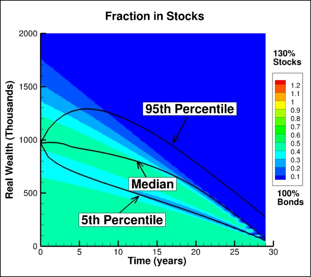
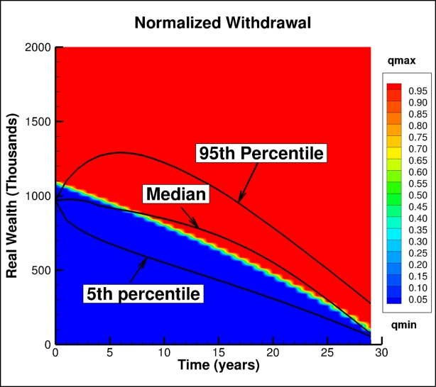
In order to gain some insight into the optimal controls, we plot the heat maps of the optimal asset allocation and the optimal withdrawals, for the cases in Figures 4, 5, 6. For each case, we choose the point on the efficient frontier so that , since this is an interesting point on the efficient frontier.
First, note that Figures 4(b), 5(b) and 6(b) show that the optimal withdrawal strategies for a wide range of are very similar. In all cases, the withdrawal control is approximately bang-bang, that is, the optimal policy is only to withdraw the maximum or minimum amounts. In the continuous withdrawal limit, the withdrawal control can be proven to be bang-bang, Forsyth (2022). We have been unable to prove that this property holds for discrete withdrawals. However, numerical studies appear to show that the transition zone between and becomes smaller as the grid is refined. We conjecture that the true converged withdrawal control is bang-bang even for discrete rebalancing/withdrawals. The lefthand plots of Figures 4, 5, 6 show the optimal allocation strategies. We use the same colour scale for all plots, with the maximum allocation to stocks being 130%. It is interesting to see that the allocation strategies are quite similar as long as we restrict attention to the areas in the heat maps above the 5th wealth percentile. Large differences in the allocation appear below the 5th wealth percentile.


9.4 Percentiles Versus Time: Synthetic Market
Figures 7. 8 and 9 show the percentiles of fraction in stocks, wealth, and withdrawals versus time. We select the point on the efficient frontier for each case so that .
Rather surprisingly, the percentiles fraction in stocks and percentiles wealth are very similar, for all values of . However, we do see some differences in the withdrawal percentiles (the rightmost panel in each plot). The median withdrawal is slower to increase to the maximum for compared to the case with .
In addition, we can see that even for , the 95th percentile for stock allocation is less than (Figure 7(a)), suggesting that with this level of ES risk, the optimal policy rarely allocates a large fraction to stocks.


10 Bootstrap results
10.1 Historical Market
In order to check on the robustness of the above results, we proceed as follows. We compute and store the optimal controls based on the parametric model (3-4) as for the synthetic market case. However, we compute statistical quantities using the stored controls, but using bootstrapped historical return data directly. In this case, we make no assumptions concerning the stochastic processes followed by the stock and bond indices. We remind the reader that all returns are inflation-adjusted. We use the stationary block bootstrap method (Politis and Romano, 1994; Politis and White, 2004; Patton et al., 2009; Cogneau and Zakalmouline, 2013; Dichtl et al., 2016; Cavaglia et al., 2022; Simonian and Martirosyan, 2022; Anarkulova et al., 2022).
A key parameter is the expected blocksize. Sampling the data in blocks accounts for serial correlation in the data series. We use the algorithm in Patton et al. (2009) to determine the optimal blocksize for the bond and stock returns separately, see Table 5. However, in our simulations, we use a paired sampling approach to simultaneously draw returns from both time series. In this case, a reasonable estimate for the blocksize for the paired resampling algorithm would be about years. We will give results for a range of blocksizes as a check on the robustness of the bootstrap results. Detailed pseudo-code for block bootstrap resampling is given in Forsyth and Vetzal (2019).
Optimal expected block size for bootstrap resampling historical data
| Data | Optimal expected |
|---|---|
| block size (months) | |
| 30-day T-bill | 51 |
| CRSP cap weighted index | 4.0 |
Figure 10 plots (i) the synthetic efficient frontier and (ii) bootstrap efficient frontier, computed using the synthetic market controls, tested in the historical market, for various blocksizes. Figure 10(a) shows the results for . In this case, all the frontiers are quite close, especially compared to the Bengen (1994) strategy, tested in the historical market. The effect of using different expected blocksizes in the block bootstrap algorithm is quite small. Overall, this plot suggests that the optimal controls in this case are robust to model parameter misspecification.
The historical test for is shown in Figure 10(b). Again, the historical frontiers using different blocksizes are quite close. However, the historical efficient frontiers do deviate somewhat from the synthetic market frontier, for values of . This indicates that there is some effect of model parameter misspecification, for large values of in the case of . However, for values of , the synthetic and historical market frontiers are very close. So, unless the retiree is extremely risk averse, this may not be a problem of practical concern.


Figures 11 and 12 show the percentiles of fraction in stocks, wealth, and optimal withdrawals, tested in the historical market. The two extreme cases: and are shown.
The percentiles in stocks and wealth are fairly close, for both cases. However, a comparison of Figures 11(c) and Figure 12(c) indicates that the median withdrawal increases from the minimum to the maximum over about three years for the case with . The comparable time frame for is about four years.
Although most retirees would prefer larger withdrawals during the early years of retirement, slightly lower initial withdrawals in exchange for never having more than 50% stock allocation might be seen as a reasonable tradeoff.


11 Limitations of the Methods Used
We should note the following limitations of the PIDE-Fourier methods used in this Chapter.
-
•
PIDE methods (in general) are limited to problems with no more than three stochastic factors. This excludes a number of problems of interest, for example portfolios having more than three risky assets, and adding stochastic mortality.
-
•
Fourier based approaches require stochastic processes which have known, closed form expressions for the Fourier transform of the Green’s function (equivalently the characteristic function).
-
•
In order to ensure -monotonicity, piecewise linear basis functions are used. This caps the rate of convergence (for smooth functions) at second order in the grid spacing. This contrasts with the Chebyshev (Gaßet al., 2018; Glau et al., 2019) or Fourier based COS method (Fang and Oosterlee, 2008; 2009; Ruijter et al., 2013) which, assuming smoothness, can achieve exponential convergence in some cases. But these techniques are not guaranteed to satisfy the -monotonicity property needed to prove convergence. We also note that it is non-trivial to obtain high order convergence even for American options (Ruijter et al., 2013), due to the jump in the second derivative across the exercise boundary. Careful tracking of the exercise boundary is necessary. These methods would be difficult to implement for general optimal control problems.
At the same time these limitations are counterbalanced by the ability to obtain provably convergent solutions to complex control problems, with realistic constraints.
Finally we should mention a recent approach for high dimensional stochastic control which is based on approximating the control by a neural network. This machine learning technique (Li and Forsyth, 2019; Van Staden et al., 2023; 2024; Chen et al., 2025) is purely data-driven, and makes no assumptions about the underlying stochastic processes. However, this also comes with the caveat that convergence proofs require determination of the global minimum of a non-convex function, which is problematic in practice.
12 Conclusions
In this paper, we have developed a technique for solving the optimal control problem associated with decumulation of a defined benefit (DC) pension plan. The basic control algorithm at each rebalancing time consists of (i) solution of an optimization problem and (ii) advancing the solution to the next rebalancing time (going backwards). We use a -monotone scheme, based on Fourier methods, for step (ii). This method preserves order relations to , which is an important property for numerical solution of optimal control. We pay particular attention to ensuring that the Fourier wrap-around error can be made arbitrarily small.
From a practical point of view, we have verified that the controls are robust by testing the controls using block bootstrap resampling of historical data, which makes no assumptions about stochastic processes for the underlying stock and bond indexes.
Perhaps the most interesting result, in terms of investment strategies for retirees, is the following. If the maximum fraction in equities is restricted to be less than 50%, this strategy is only slightly less efficient than allowing a maximum fraction of 130% (that is, using leverage). This suggests that for most retirees, there is no need to undertake risky strategies during the decumulation of a DC account.
These optimal control strategies are far more efficient than the typical four percent rule (Bengen, 1994). The optimal policy has an expected average withdrawal (real) of more than 5% of initial capital over thirty years, with approximately zero expected shortfall at age 95 (based on historical data). In contrast, the strategy suggested in (Bengen, 1994), withdraws 4% of initial capital annually, but has an expected shortfall of more than 35% of initial capital at age 95.
Appendices
13 Wrap Around Error: Details
To gain some insight into the wrap-around problem, we consider a highly simplified, one dimensional problem. To avoid subscript clutter, in this section, we use the notation
Using the above notation, consider the discrete time advance convolution
| (60) | |||||
where we assume periodic extension of
In the above, if , nodes corresponding to and are the padded nodes. In this case, we assume that the padded nodal values , and , are determined by boundary data.
As an example of wrap-around error, we examine a worst case term in equation (60). Consider the term in (60) corresponding to , and , namely
| (61) |
By periodic extension, we shift the argument of by , resulting in
| (62) |
and hence, the term (61) becomes
| (63) |
Hence, in this extreme case, equation (60) becomes
| (64) |
Example 1(No padding: )
Suppose we do not use any padding, so that In this case, equation (64) becomes
Since, in general, is not small, we can see that the term has a considerable effect on , which should not be the case. We can see here that the periodic extension of causes a wrap-around effect.
Example 2(Padding: )
13.1 Wrap-around: a formal result
From our previous examples, we can see that wrap-around may occur in equation (60) if
This leads us to the following formal definition of wrap-around error. We show that, with , wrap-around error is sufficiently reduced.
Definition 2(Wrap-around error)
Assume is periodic with period and , for or , are determined by boundary data with . Then the wrap-around error for equation (60), at timestep , denoted by , is
We can now state the following result.
Theorem 13.1
Let be periodic with period and , for or , be determined by boundary data with . Assume further that is bounded, so for , there exists a positive constant such that121212This is essentially a stability condition. See Forsyth and Labahn (2019) for a proof of stability for the -monotone method.
| (67) |
If is selected sufficiently large so that
| (68) |
then the wrap-around error after steps is bounded by .
Proof
Applying property (67) to equation (LABEL:wrap_error_1) gives
| (69) |
Recall that , hence the worst case values of on the righthand side of equation (69) are and . Thus equation (69) gives
| (70) | |||||
Also, since equation (70) becomes
| (71) | |||||
and eliminating the indicator functions gives
Shifting by so that the argument of is in the range , implies
| (72) | |||||
Rearranging the indices, gives
| (73) |
which, since , implies that equation (73) satisfies
| (74) |
Since
| (75) |
then
| (76) | |||||
| (77) |
where the last step follows from condition (68). Applying equation (77) recursively gives the bound .
It might at first sight seem odd to weaken the error bound using equation (75). However, this makes the final result easy to interpret. Let
| (78) |
so that is the set of node indexes for the padded domain, and is the set of node indices for the original domain. Consequently, condition (76) can be written compactly as
| (79) |
Proving Theorem 8.1 basically follows the previous proof of the simpler case. Divide the region outside into right and left and upper and lower regions as follows.
Our goal is to give an upper bound to
which by the boundedness assumptions of Theorem 8.1 is the same as bounding
As in the 1d wraparound error, our worse case values occur at borders, in this case the four corners of . In the horizontal direction when the first components are and we can use the same manipulations as done in the 1d case to obtain the wraparound error contribution from and and use an identical argument when the second argument is and to get the wraparound error contribution from and . These manipulations reduce to
for each time step and hence give the error bound after steps.
References
- Alonso-Garcca et al. (2018) Alonso-Garcca, J., O. Wood, and J. Ziveyi (2018). Pricing and hedging guaranteed minimum withdrawal benefits under a general Lévy framework using the COS method. Quantitative Finance 18, 1049–1075.
- Anarkulova et al. (2022) Anarkulova, A., S. Cederburg, and M. S. O’Doherty (2022). Stocks for the long run? Evidence from a broad sample of developed markets. Journal of Financial Economics 143:1, 409–433.
- Anarkulova et al. (2025) Anarkulova, A., S. Cederburg, M. S. O’Doherty, and R. W. Sias (2025). The safe withdrawal rate: Evidence from a broad sample of developed markets. Journal of Pension Economics and Finance 24:3, 464–500.
- Barles and Souganidis (1991) Barles, G. and P. Souganidis (1991). Convergence of approximation schemes for fully nonlinear equations. Asymptotic Analysis 4, 271–283.
- Bengen (1994) Bengen, W. (1994). Determining withdrawal rates using historical data. Journal of Financial Planning 7, 171–180.
- Bjork et al. (2021) Bjork, T., M. Khapko, and A. Murgoci (2021). Time inconsistent control theory with finance applications. New York: Springer Finance.
- Cavaglia et al. (2022) Cavaglia, S., L. Scott, K. Blay, and S. Hixon (2022). Multi-asset class factor premia: A strategic asset allocation perspective. The Journal of Portfolio Management 48:9, 14–32.
- Chen et al. (2025) Chen, M., M. Shirazi, P. A. Forsyth, and Y. Li (2025). Machine learning and Hamilton-Jacobi-Bellman equation for optimal decumulation: a comparison study. Journal of Computational Finance 29:1, 77–118.
- Cogneau and Zakalmouline (2013) Cogneau, P. and V. Zakalmouline (2013). Block bootstrap methods and the choice of stocks for the long run. Quantitative Finance 13, 1443–1457.
- Cont and Mancini (2011) Cont, R. and C. Mancini (2011). Nonparametric tests for pathwise properties of semimartingales. Bernoulli 17, 781–813.
- Cui et al. (2022) Cui, X., D. Li, X. Qiao, and M. Strub (2022). Risk and potential: An asset allocation framework with applications to robo-advising. Journal of the Operations Research Society of China 10, 529–558.
- Dang and Forsyth (2016) Dang, D.-M. and P. A. Forsyth (2016). Better than pre-commitment mean-variance portfolio allocation strategies: a semi-self-financing Hamilton-Jacobi-Bellman equation approach. European Journal of Operational Research 250, 827–841.
- Dichtl et al. (2016) Dichtl, H., W. Drobetz, and M. Wambach (2016). Testing rebalancing strategies for stock-bond portfolios across different asset allocations. Applied Economics 48, 772–788.
- Fang and Oosterlee (2008) Fang, F. and C. Oosterlee (2008). A novel pricing method for European options based on Fourier cosine series expansions. SIAM Journal on Scientific Computing 31, 826–848.
- Fang and Oosterlee (2009) Fang, F. and C. Oosterlee (2009). Pricing early-exercise and discrete barrier options by Fourier cosine series expansions. Numerische Mathematik 114, 27–62.
- Forsyth and Labahn (2019) Forsyth, P. and G. Labahn (2019). -Monotone Fourier methods for optimal stochastic control in finance. Journal of Computational Finance 22:4, 25–71.
- Forsyth (2020a) Forsyth, P. A. (2020a). Multi-period mean CVAR asset allocation: Is it advantageous to be time consistent? SIAM Journal on Financial Mathematics 11:2, 358–384.
- Forsyth (2020b) Forsyth, P. A. (2020b). Optimal dynamic asset allocation for DC plan accumulation/decumulation: Ambition-CVAR. Insurance: Mathematics and Economics 93, 230–245.
- Forsyth (2022) Forsyth, P. A. (2022). A stochastic control approach to defined contribution plan decumulation: “The Nastiest, Hardest Problem in Finance”. North American Actuarial Journal 26:2, 227–252.
- Forsyth and Vetzal (2019) Forsyth, P. A. and K. R. Vetzal (2019). Optimal asset allocation for retirement savings: deterministic vs. time consistent adaptive strategies. Applied Mathematical Finance 26:1, 1–37.
- Forsyth et al. (2020) Forsyth, P. A., K. R. Vetzal, and G. Westmacott (2020). Optimal asset allocation for a DC pension decumulation with a variable spending rule. ASTIN Bulletin 50:2, 419–447.
- Forsyth et al. (2022) Forsyth, P. A., K. R. Vetzal, and G. Westmacott (2022). Optimal control of the decumulation of a retirement portfolio with variable spending and dynamic asset allocation. ASTIN Bulletin 51:3, 905–938.
- Garroni and Menaldi (1992) Garroni, M. G. and J. L. Menaldi (1992). Green functions for second order parabolic integro-differential problems. New York: Longman Scientific.
- Gaßet al. (2018) Gaß, M., K. Grau, M. Mahlstedt, and M. Mair (2018). Chebyshev interpolation for parametric option pricing. Finance and Stochastics 22, 701–731.
- Glau et al. (2019) Glau, K., M. Mahlstedt, and C. Potz (2019). A new approach for American option pricing: the dynamic Chebyshev method. Siam Journal on Scientific Computing 41, B153–B180.
- Ignatieva et al. (2018) Ignatieva, K., A. Song, and J. Ziveyi (2018). Fourier space timestepping algorithm for valuing guaranteed minimum withdrawal benefits in variable annuities under regime switching and stochastic mortality. ASTIN Bulletin 48, 139–169.
- Kou (2002) Kou, S. G. (2002). A jump-diffusion model for option pricing. Management Science 48, 1086–1101.
- Kou and Wang (2004) Kou, S. G. and H. Wang (2004). Option pricing under a double exponential jump diffusion model. Management Science 50, 1178–1192.
- Li and Forsyth (2019) Li, Y. and P. Forsyth (2019). A data-driven neural network approach to optimal asset allocation for target based defined contribution pension plans. Insurance: Mathematics and Economics 86, 189–204.
- Lin et al. (2015) Lin, Y., R. MacMinn, and R. Tian (2015). De-risking defined benefit plans. Insurance: Mathematics and Economics 63, 52–65.
- Lippa (2013) Lippa, J. (2013). A Fourier space time-stepping approach to problems in finance. MMath thesis, University of Waterloo.
- MacDonald et al. (2013) MacDonald, B.-J., B. Jones, R. J. Morrison, R. L. Brown, and M. Hardy (2013). Research and reality: A literature review on drawing down retirement financial savings. North American Actuarial Journal 17, 181–215.
- MacMinn et al. (2014) MacMinn, R., P. Brockett, J. Wang, Y. Lin, and R. Tian (2014). The securitization of longevity risk and its implications for retirement security. In O. S. Mitchell, R. Maurer, and P. B. Hammond (Eds.), Recreating Sustainable Retirement, pp. 134–160. Oxford: Oxford University Press.
- Mancini (2009) Mancini, C. (2009). Non-parametric threshold estimation models with stochastic diffusion coefficient and jumps. Scandinavian Journal of Statistics 36, 270–296.
- Menoncin and Vigna (2017) Menoncin, F. and E. Vigna (2017). Mean-variance target based optimisation for defined contribution pension schemes in a stochastic framework. Insurance: Mathematics and Economics 76, 172–184.
- Patton et al. (2009) Patton, A., D. Politis, and H. White (2009). Correction to: automatic block-length selection for the dependent bootstrap. Econometric Reviews 28, 372–375.
- Peijnenburg et al. (2016) Peijnenburg, K., T. Nijman, and B. J. Werker (2016). The annuity puzzle remains a puzzle. Journal of Economic Dynamics and Control 70, 18–35.
- Pfeiffer et al. (2013) Pfeiffer, S., J. R. Salter, and H. E. Evensky (2013). Increasing the sustainable withdrawal rate using the standby reverse mortgage. Journal of Financial Planning 26:12, 55–62.
- Politis and Romano (1994) Politis, D. and J. Romano (1994). The stationary bootstrap. Journal of the American Statistical Association 89, 1303–1313.
- Politis and White (2004) Politis, D. and H. White (2004). Automatic block-length selection for the dependent bootstrap. Econometric Reviews 23, 53–70.
- Ritholz (2017) Ritholz, B. (2017). Tackling the ‘nastiest, hardest problem in finance’. www.bloomberg.com/view/articles/2017-06-05/tackling-the-nastiest-hardest-problem-in-finance.
- Rockafellar and Uryasev (2000) Rockafellar, R. T. and S. Uryasev (2000). Optimization of conditional value-at-risk. Journal of Risk 2, 21–42.
- Ruijter et al. (2013) Ruijter, M. J., C. W. Oosterlee, and R. Albers (2013). On the Fourier cosine series expansion method for stochastic control problems. Numerical Linear Algebra and Applications 20, 598–625.
- Shefrin and Thaler (1988) Shefrin, H. M. and R. H. Thaler (1988). The behavioral life-cycle hypothesis. Economic Inquiry 26, 609–643.
- Simonian and Martirosyan (2022) Simonian, J. and A. Martirosyan (2022). Sharpe parity redux. The Journal of Portfolio Management 48:9, 183–193.
- Strub et al. (2019) Strub, M., D. Li, X. Cui, and J. Gao (2019). Discrete-time mean-CVaR portfolio selection and time-consistency induced term structure of the CVaR. Journal of Economic Dynamics and Control 108. Article 103751 (electronic).
- Thinking Ahead Institute (2024) Thinking Ahead Institute (2024). Global pension assets study 2024. https://www.thinkingaheadinstitute.org/content/uploads/2024/02/GPAS-2024.pdf.
- Van Staden et al. (2018) Van Staden, P. M., D.-M. Dang, and P. Forsyth (2018). Time-consistent mean-variance portfolio optimization: a numerical impulse control approach. Insurance: Mathematics and Economics 83, 9–28.
- Van Staden et al. (2023) Van Staden, P. M., P. A. Forsyth, and Y. Li (2023). Beating a benchmark: dynamic programming may not be the right numerical approach. SIAM Journal on Financial Mathematics 14(2), 407–451.
- Van Staden et al. (2024) Van Staden, P. M., P. A. Forsyth, and Y. Li (2024). A global-in-time neural network approach to dynamic portfolio optimization. Applied Mathematical Finance 31:3, 131–163.
- Vigna (2014) Vigna, E. (2014). On efficiency of mean-variance based portfolio selection in defined contribution pension schemes. Quantitative Finance 14, 237–258.
- Vigna (2022) Vigna, E. (2022). Tail optimality and preferences consistency for intertemporal optimization problems. SIAM Journal on Financial Mathematics 13(1), 295–320.