The impact of flickering variability and magnetisation on the dynamics, stability and morphology of radio-loud AGN jets
Abstract
The physics governing the morphology of radio-loud AGN jets is not fully understood. We investigate how magnetization, flickering jet power and their interplay affects the morphology of radio galaxies. We present a grid of relativistic magnetohydrodynamic simulations using the PLUTO code covering constant and variable jets with two levels of magnetisation. We find that the constant high magnetisation jets can lead to highly asymmetrical cocoon morphologies, whilst the variable high magnetisation jet can exhibit a broken morphology, caused by a discontinuous jet beam. Our work highlights the importance of magnetisation and variability on the stability and resulting morphology of radio-loud AGN jets, suggesting both are significant factors in addition to jet power or environment. Furthermore, we show that the interaction between magnetisation and variability can lead to the development of localised kink instabilities along the jet beam. Finally, we discuss the effects of hydrodynamic mixing in low magnetisation jets and the role of viewing angle dependence in comparisons between our simulations and observed sources. To facilitate this comparison we present a library of simulated radio images at different times in the simulations and from various viewing angles, which highlight a diverse set of complex morphologies.
keywords:
galaxies: jets – radio continuum: galaxies – (magnetohydrodynamics) MHD – instabilities – software: simulations – relativistic processes1 Introduction
Observations of radio jets from AGN show a large amount of morphological diversity, with possible causes of differences in age, environment, magnetisation and power. Classically, radio galaxies have been divided into Fanaroff and Riley I and II morphologies (Fanaroff and Riley, 1974), describing centre-brightened and edge-brightened morphologies respectively. Large-scale surveys such as LoTSS (Shimwell et al., 2022) have revealed a wealth of jet morphologies, with many sources displaying S- and C-shaped curvatures, multiple hotspots or jets misaligned from the central axis (e.g. Horton et al., 2025). Moreover, individual nearby sources observed with high spatial resolutions show a wealth of features. For example, Cygnus A (Carilli et al., 1989) features a misaligned jet and multiple hotspots, 3C 98 has a misaligned jet together with a one-sided backflow (Leahy et al., 1997), and IC 4296 (Condon et al., 2021) shows a clear break in the emissivity of the Western jet combined with a helical structure. Understanding the drivers behind how this diversity in structures is formed is critical to understanding the properties of radio galaxies, both within an individual source and across populations. Crucially, if we can understand their formation, the various morphologies and jet structures provide an opportunity to study AGN duty-cycles, feedback and jet launching physics over timescales of Myr.
Observations of individual sources give us an insight into a snapshot of the jet’s evolution, whereas population-based studies allow us to understand how common various morphologies are. Simulations, then, are a vital tool in advancing our understanding of how various morphologies come to exist, and under which conditions their formation is possible. As an illustration of this, simulations of constant power magnetised jets often display asymmetrical features over large length scales, including various combinations of jet bending, complex hotspot morphologies and one-sided backflows (e.g. Hardee and Norman, 1990; Cox et al., 1991; English et al., 2016; Perucho et al., 2019; Mukherjee et al., 2020; Meenakshi et al., 2023; Rossi et al., 2024). Higher magnetisations have been shown to stabilise jets with respect to Kelvin-Helmholtz (KH) instabilities and reduce entrainment, although being cold and fast can also lengthen the growth timescales of KH instabilities (e.g. Perucho et al., 2010). Rossi et al. (2024) showed that deceleration due to entrainment is reduced in jets with higher magnetisations, enabling the creation of FR II-like morphologies at jet powers of approximately , whereas lower magnetisation jets with the same power undergo significant entrainment and deceleration, suggesting the formation of FRI-like morphologies (see also Rossi et al., 2008). At the same time, increasing magnetisation reduces stability to current-driven kink instabilities (Appl et al., 2000), resulting in the formation of helical patterns in the jet beam (e.g. Mukherjee et al., 2020; Rossi et al., 2024). Tchekhovskoy and Bromberg (2016) investigated the potential role of the kink instability in producing the Fanaroff-Riley Dichotomy using 3D MHD simulations, finding it may play an important role, whereas Musso et al. (2024) studied the stability of more idealised sections of pressure-balanced jets. Furthermore, instability to the kink mode leads to magnetic reconnection which can provide an additional mechanism by which to accelerate electrons in a jet to non-thermal energies (e.g. Davelaar et al., 2020; Musso et al., 2024).
Whilst magnetisation is known to be a key factor in determining the stability and dynamics of astrophysical jets, variability is also likely to have significant impacts. Variability in AGN jets is directly observed on short timescales (for a review, see Raiteri, 2025, and references therein). It is expected that AGN jets also vary over very long time scales – sources such as Hercules A are often explained with restarting jets (e.g. Timmerman et al., 2022), and AGN jets are expected to be influenced by (and to influence) merger activity (e.g. Talbot et al., 2024). Further to this, theories such as chaotic cold accretion (CCA, King and Pringle, 2006; Gaspari et al., 2013) suggest that the accretion rate should vary on timescales of fractions of a Myr with a lognormal distribution of powers and obeying a pink noise spectrum (Gaspari et al., 2017). This is the behaviour we describe as flickering.
In Elley et al. (2026) we investigated flickering jets using relativistic hydrodynamic (RHD) simulations, finding that moderate changes in Lorentz factor on timescales of a fraction of a Myr could create large short-lived increases in synchrotron luminosity. However, variability is of course not limited to flickering – in the context of restarting jets Barniol Duran et al. (2017), found that stability to the kink mode can be greatly affected by previous epochs of jet activity. Furthermore, variability can also refer to changes to variables other than a jet’s power – Chen et al. (2023) study the evolution of magnetised jets, including a jitter in the initial launch angle of the jets. The magnetised jets with jitter display complex morphologies with large scale twisting magnetic field structures directly imprinted by the varying jet direction.
To summarise, previous work has suggested that both variability and magnetisation can have significant effects on the morphologies and stability of AGN jets, and that variability in the morphologies and luminosities of individual jets may contribute strongly to the observed diversity of sources. In particular, some degree of flickering variability is an expected consequence of accretion theories and can lead to variability in jet morphology in non-magnetised jets. In order to exploit the potential information encoded within jet morphologies, it is necessary to develop a detailed understanding of the possible ways in which jets with different magnetisations and variability properties can evolve. As of yet, no systematic investigation has been carried out on the interplay between variability and magnetisation and their joint impacts on the jet-lobe system. In this work, we study this combination of flickering variability with dynamically important magnetic fields and assess consequences for the expected morphologies of powerful radio sources. We use a grid of simulations with and without variability, and with low and high magnetisations to separate the effects of each property.
We describe our simulations in Section 2, paying particular attention to the model of a magnetised jet used, together with the specific properties of the variability. In Section 3, we discuss the results of the simulations, giving an overview of the results from the high magnetisation, variable power jet in Section 3.1, before focusing on large-scale asymmetries in Section 3.2, and on the formation of discontinuities in the jet beam in Section 3.3. In Section 4, we discuss the stability of our injected jet model to kink instabilities and how this governs the formation of helical structures and localised kink structures in the jets. Section 5 presents simulated radio images made using the simulations, together with a discussion of viewing angle effects, light travel time effects and comparisons with observations of specific sources. We conclude in Section 6.
2 Methods
2.1 Simulation setup
We run 3D RMHD simulations of jets with both constant and varying power using the PLUTO code Mignone et al. (2007). The domain of each simulation is and consists of cells, giving a resolution of 40 pc per cell in each direction. We inject a jet along the axis.
| Power | Magnetisation | |
|---|---|---|
| Constant | Low | 0.001 |
| Constant | High | 0.01 |
| Variable | Low | 0.001 |
| Variable | High | 0.01 |
The variable jets have powers which obey a lognormal probability density function
| (1) |
where is the jet power at any given time, is the median jet power and the standard deviation of the natural logarithm of the jet powers is 0.33. The jet power time series has a pink noise power spectrum (power spectral density ). We generate the time series for the jet power using DELightcurveSimulation (Connolly, 2016) which is an implementation of the Emmanoulopoulos light curve simulation algorithm (Emmanoulopoulos et al., 2013). The grid of simulations consists of 4 runs with varying combinations of magnetisation and variability as shown in Table 1. The variable simulations use the same random noise seed as Seed 6 as in Elley et al. (2026).
We use linear reconstruction, second-order Runge-Kutta time-stepping and the Taub-Mathews Equation of State (Mathews, 1971). The divergence-free condition is maintained through divergence cleaning. Away from strong shocks, we use the Harten–Lax–van Leer Riemann (HLLD) solver of Mignone et al. (2009) with the monotonized central difference limiter. We use the multidimensional (MULTID) shock identification and flattening strategy, where for strong shocks above a threshold of (where is the gas pressure), the (diffusive) minmod limiter is used for reconstruction and the Harten–Lax–van Leer (HLL) Riemann solver is used. This forces the simulation to be more dissipative around shocks, but is required for numerical stability.
Initially the ambient density is set to a King profile,
| (2) |
with a core radius, , of 50 kpc, and with and g cm-3. is equivalent to a proton number density of and our values for , and are broadly consistent with typical values for host galaxies of radio-loud AGN (e.g. Ineson et al., 2015) . Small perturbations are added to this density profile to remove the exact symmetry of the simulation. The pressure of the ambient medium is set to a low value and our results are not sensitive to this choice until the sound speed is very high. For numerical reasons, we set the magnetic field in the background to a small but non-zero, dynamically negligible constant value, in a direction perpendicular to the jet axis (See Appendix A). A more realistic background field is outwith the scope of this work –we focus on the field structures developing within the jet. The bow shock ensures that the low magnitude magnetic field structure in the ambient medium has little effect on the internal magnetic field structures.
We use outflow boundary conditions on all sides, except the side through which the jet enters the simulation; this boundary is set to be reflective everywhere but the jet nozzle. We inject a jet with a density of g cm-3 through a nozzle of radius kpc. We discuss the remaining boundary conditions for the jet in Section 2.2.
2.2 Jet model
We simulate an underdense jet with a toroidal magnetic field. The jet is initially in radial equilibrium, which requires the specification of a magnetic field (Section 2.2.1) and pressure profile (Section 2.2.3) within the jet. In order to create a jet with the required power at a given level of magnetisation (Section 2.2.4), we vary the Lorentz factor as described in Section 2.2.5. We use the convention that primed quantities are as measured in the rest frame of the fluid throughout.
2.2.1 Magnetic field structure
We choose a toroidal field structure adhering to some general constraints, namely that the field must have zero divergence () and not result in a singularity at the centre of the jet (). Furthermore, we stipulate that the field strength must fall off to a small value at the outer radius of the jet. This avoids a large step change at the outer radius, improving numerical stability and is a reasonable physical expectation. The simplest non-trivial structure obeying these constraints is a field that reaches a maximum strength at some critical cylindrical radius within the jet, before decreasing in strength with further increasing radius. We make the choice that and describe fields that reach a maximum strength at this point. Whilst the exact profiles and value of are specific choices, we note that other reasonable choices are unlikely to greatly alter the overall qualities of our results. To motivate this expectation, we analyse the stability of this outer region of the jet in Appendix D, showing that for the same small displacement from the equilibrium, the resulting forces on the outer region are much smaller than those experienced by the central region (an analysis of which can be found in Section 4.1).
Within the radius , we inject a toroidal field with
| (3) |
and . Outside of the radius we use a field with
| (4) |
and again . The two field profiles result in an equal strength at . For , the field given above has a decreasing strength with radius, to a low value at . The Cartesian versions of these fields and the smoothing function used at the outer radius of the injected jet, , are described in Appendix A.
2.2.2 Equilibria
The field structure discussed in Section 2.2.1 results in a magnetic pressure inwards on the jet, so to create an equilibrium this force must be balanced by either rotation of the jet or a pressure gradient, as shown below. As we focus on simulating jets on scales of kpc to tens of kpc in this work, which are scales at which the jet material is distant from the jet launching region and at which the jet is expected to have already transformed most of its Poynting flux to thermal and kinetic energy, we focus on equilibria supported purely by pressure balance (e.g. Musso et al., 2024).
For a steady-state jet assuming ideal magnetohydrodynamics (MHD) with negligible resistivity, the condition for an equilibrium state is given by
| (5) |
where we have used the assumption that and vary only in the direction. The first and second terms represent the gradients of the thermodynamic and magnetic pressures respectively and the third the centripetal force needed to maintain a circular rotation (if the toroidal velocity were non-zero). In this work we consider non-rotating jets, such that . Furthermore, in ideal MHD, the fluid is perfectly conductive such that
| (6) |
For a non-rotating jet where the velocity does not vary with radius, there is a co-moving frame where throughout a slice of the jet, such that the electric field in the co-moving frame is zero. To convert between the rest frame and comoving frame toroidal fields, we note that the toroidal component of the magnetic field in the observer frame is
| (7) |
assuming .
2.2.3 Pressure profile
In the observer frame, Equation 5 can be written as
| (8) |
For , this necessitates a constant pressure with changing radius. For , we obtain a similar result to Mignone et al. (2013) for the required thermal pressure at a given time:
| (9) |
We follow Mignone et al. (2013) in defining the constant such that the jet pressure matches the ambient pressure at a radius .
| (10) |
2.2.4 Magnetisation
We adopt the usual definition (e.g. Mukherjee et al., 2020) of the jet magnetisation as the ratio between the Poynting flux, , and the enthalpy density flux, ,
| (11) |
where is the relativistic enthalpy density of the jet, given by
| (12) |
according to the Taub-Mathews Equation of State (Mathews, 1971). We neglect the rest mass contribution to the enthalpy flux. The peak value of the magnetisation occurs at and is given by
| (13) |
In the variable jet power simulations we hold the injected lab frame magnetic field strength constant, leading to a varying magnetisation.
2.2.5 Lorentz factor from the power of the jet
The jet power is given by the integral of the total enthalpy flux over the area of the jet nozzle, including the magnetic field contribution, and is given by
| (14) |
where the ‘in’ and ‘out’ subscripts refer to the quantities within and respectively. Substituting in the expressions for the Poynting and enthalpy fluxes (see Equation 11), and again neglecting the contribution from the rest mass energy to the enthalpy flux, gives
| (15) |
To parametrise our jets, we specify the mean jet power, , together with the peak magnetisation at this mean jet power, which we denote . Equation 13 specifies the comoving peak toroidal magnetic field strength, which is independent of Lorentz factor. This can then be substituted into Equation 15 with the appropriate Lorentz transformation to find the power of a jet with this comoving magnetic field strength. To invert Equation 15, we tabulate the power for a range of Lorentz factors using Equation 15 and use this data as a look-up table to find the Lorentz factor as a function of power. Figure 1 shows the jet power as a function of Lorentz factor for various levels of magnetisation.

It is notable that for the magnetisations we use (, as shown in Table 1), the jet power depends only very weakly on the magnetisation. This justifies our choice to use the magnetisation at the mean jet power to calculate the Lorentz factor for all Lorentz factors. Figure 2 shows the Lorentz factors calculated using the method.

An alternative possible choice would be to hold the magnetisation constant and instead vary the injected toroidal magnetic field strength in the lab frame. In this case, the comoving injected toroidal field would remain constant, and therefore the injected pressure would also be held constant in time.
2.3 Production of rendered emissivity images
As part of our work, we also create predictions of observed synchrotron images with an approximate treatment of the synchrotron emissivity of the plasma. We do this from various angles to the line of sight to illustrate the effects of Doppler boosting on the appearance of the jets. To produce the emissivity images from different angles, we first transform the magnetic fields to the co-moving frame for each cell, then calculate rest frame emissivity estimates for each cell. We use the prescription that pseudo-emissivity (in the rest frame) is given by (e.g. Rybicki and Lightman, 1979)
| (16) |
where is a reference emitting frequency, is the magnetic energy density and is the jet tracer which tracks the fraction of material in a cell which entered the simulation through the jet nozzle. We do not specify an observing frequency that our simulated radio images are made at, but assume that it is low enough to be well-described by power law emission with a single slope. We assume that the electron energy density spectrum is given by a power law with an index of , and that the resulting synchrotron spectrum has an index , such that . We describe the processes of calculating the co-moving magnetic field strengths and converting them into an observed simulated radio image at a single observing frequency in further detail in Appendix C. We calculate the emergent specific intensity using an in-house ray tracing code to perform line-of-sight integration of the pseudo-emissivity in the observer frame, Doppler boosting the emissivity on a per-cell basis according to the local fluid velocity with respect to the line of sight (see Appendix C).
We simulate one jet (or one side of a radio galaxy) in each case, whereas almost all observed radio galaxies are seen to be double-sided, with one-sided jets commonly explained by strong Doppler de-boosting of the receding jet (e.g. Horton et al., 2025). To produce the double-sided jets shown in our emissivity maps we mirror the jets along the jet axis and then, for the mirrored jet, we swap the two axes perpendicular to the jet axis. We carry out this axis-swap to reduce the symmetry and allow a wider variety of views of the simulated jet overall. We do not account for light travel time effects as this would require simulation data to be saved much more often during the simulation, which is not feasible due to storage and processing limitations. We discuss light travel time effects further in Section 5.2. All scales shown in kpc on images throughout this paper are distances as projected onto the plane of the sky.
We release a set of rendered images together with this paper as FITS files. These can be found at https://doi.org/10.5281/zenodo.20140020. These cover the following views to the simulated objects:
-
1.
The jet axis remains perpendicular to the line of (). The simulation is rotated around the jet axis in degree increments.
-
2.
The angle between the jet axis and the line of sight, , is varied in 6 degree increments for a single constant azimuthal angle, .
We discuss some of the effects of viewing the same jet from different angles in Section 5.2 and videos of the highly magnetised jets can be viewed here: constant and variable.
3 Results
We discuss the broad evolution of the high magnetisation variable power jet in Section 3.1. We then move to comparing the variable high magnetisation jet to its low magnetisation and constant counterparts; this allows us to identify which features are characteristic of high magnetisation, which are characteristic of variability and which are a consequence of the interplay between the two. We summarise the key features of all the simulations in Table 2; large-scale asymmetries are discussed in Section 3.2, while discontinuous or ‘broken’ morphologies are explored in Section 3.3.
3.1 Evolution of the high magnetisation variable jet

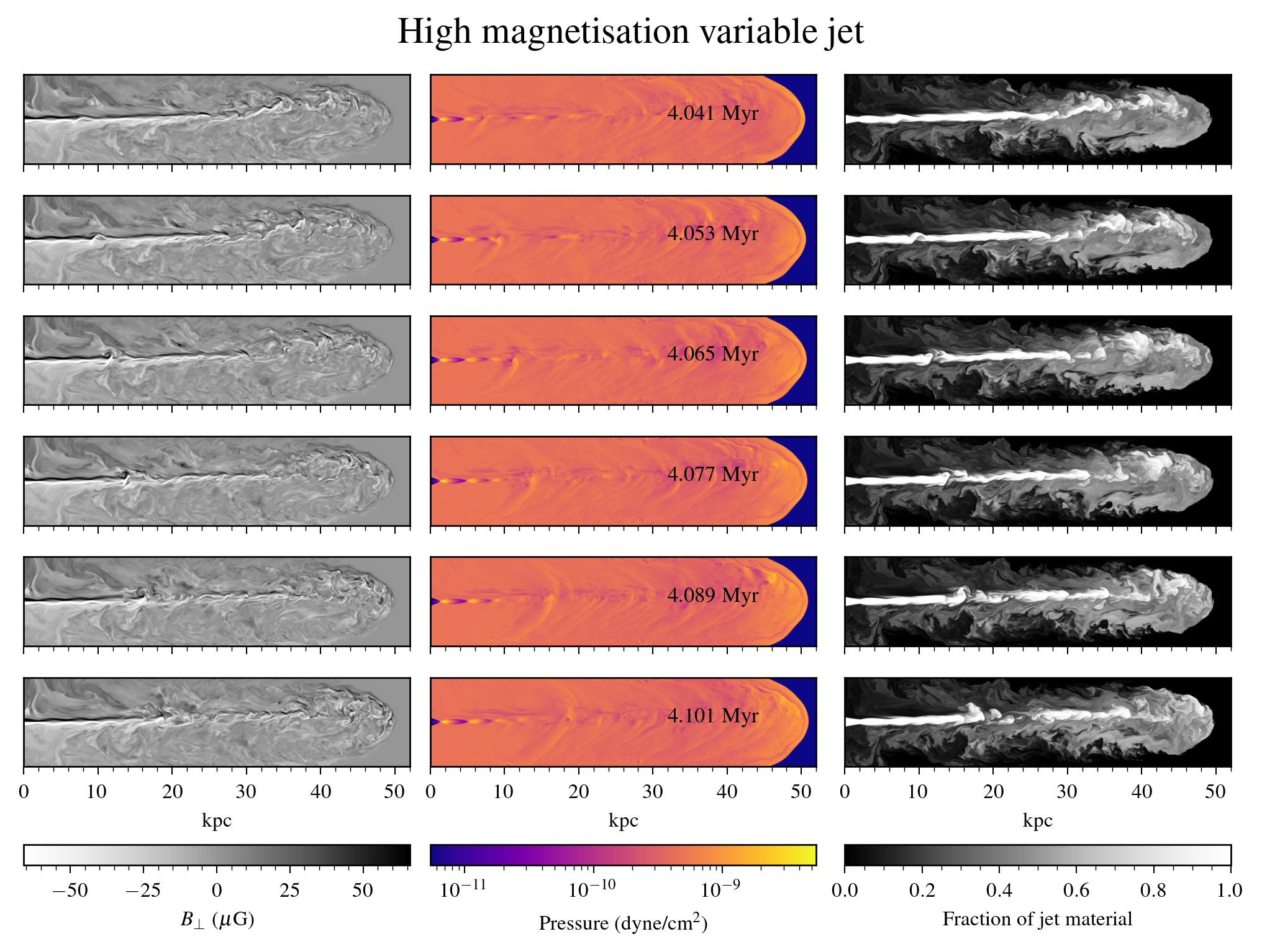
We begin by discussing the overall behaviour of the variable, high magnetisation jet simulation, which we illustrate in Figure 3. We show central slices through the full three dimensional domain of the simulation, illustrating the density, pressure, component of the magnetic field perpendicular to the slice and the jet tracer, . The figure shows the underdense, magnetised jet propagating through the majority of the 60 kpc domain in around 4 Myr, with significant variation in the cocoon shape across this time.
At 2 Myr the jet shows some large ( kpc) scale asymmetry around the jet head. This is most clearly seen in the density slice. Whilst the tracer shows the jet beam to be slightly bent away from the central axis at this time, it also shows that the jet beam appears disconnected from the head of the jet at this time, and this disconnected region coincides spatially with a more complicated structure in the magnetic field, which separates the well-defined toroidal field structure that is injected at the base from a more turbulent structure around the jet head region. In the region just before the complex break the magnetic field has small bends reminiscent of structures formed by the kink instability in previous works (e.g. Bodo et al., 2021; Meenakshi et al., 2023).
At 3 Myr the jet has experienced a recent extended period ( Myr) of relatively high power and its shape towards the jet head is narrow and pointed. The formation of this sharp, conical region is dominated by the increased ram pressure, concentrated in the area around the jet head. This behaviour was discussed in detail in the context of non-magnetised jets in Whitehead and Matthews (2023); they found that high-power periods led to increases in the ratio between jet length and the width of the bow shock at the jet base, and to decreases in the sphericity of the jet () of the jet, where is the volume enclosed by the bow shock and is the surface area of the bow shock). In this snapshot, the magnetic field structure and the tracer image both show that the jet reaches the end of the simulation domain (largely) unimpeded by instabilities. The thermal pressure at the jet head is significantly increased with respect to its value at both 2.0 and 4.0 Myr, reminiscent of the behaviour of the non-magnetised jets discussed in Elley et al. (2026), where changes in power lead to short-lived periods of dramatically brighter hotspots. The increased pressure in the highly magnetised jet shown in Figure 3 suggests that hotspot brightening as a result of changes in jet power may continue to play an important role in jets with dynamically significant magnetic field strengths.
At 4 Myr, following a period of comparatively low jet power, the cocoon shape has returned to a blunter morphology with a higher sphericity. The primary mechanism causing the development of the higher sphericity is the lateral expansion of the cocoon due to its thermal pressure, which plays a more important role than the focused ram pressure in phases of relatively low power. The thermal pressure is much more uniform across the cocoon and the effects of hydrodynamic instabilities are much more evident in the mixing of the jet material both in places along the jet beam and in the jet head area. The jet tracer shows that the jet has moved away from the central axis towards the top of the figure. In Section 3.3, we discuss the discontinuous behaviour of the highly magnetised variable jet simulation in more detail, using volume renders of the jet tracer instead of the slice shown here (see Figure 6) and we will show that the jet is in fact discontinuous at this point.
| Description | Moves off axis? | Variable morphology? | Backflows |
|---|---|---|---|
| Constant power, low magnetisation | No | constant | symmetric |
| Constant power, high magnetisation | Yes, for extended periods | variable, prominent lobe asymmetries | often one-sided |
| Variable power, low magnetisation | No | variable, travelling shocks | symmetric, vary in strength |
| Variable power, high magnetisation | Yes, for short periods | variable, broken morphology | often one-sided, clumped |
3.2 Large-scale asymmetries in high magnetisation jets
Our two high magnetisation () jet simulations exhibit departures from axisymmetry on large length scales, kpc, in agreement with previous work focusing on simulations of constant power jets with toroidal and helical fields (e.g. Mignone et al., 2010; Mukherjee et al., 2020; Chen et al., 2023; Meenakshi et al., 2023; Rossi et al., 2024). The asymmetrical behaviour we see can be grouped into two categories: (i) asymmetrical pointing of the jet beam towards one side of the lobe (misaligned jets) and (ii) asymmetries in the cocoon shape, which when they occur happen as a consequence of behaviour (i) persisting for extended periods of time. Large-scale asymmetries are not generally produced in the low magnetisation () jets, which remain approximately symmetrical on these kpc scales (e.g. Figure 13, and in agreement with the results of Chen et al. 2023).
Figure 4 shows a central slice through the toroidal magnetic field component of the high magnetisation constant power jet, at six time stamps between 1.2 and 3.2 Myr.

At around 2 Myr the jet moves away significantly from the central axis. The ram pressure of the jet is concentrated on the area immediately around the end of the jet beam and, over a period of Myr, preferentially excavates a significant volume of cocoon away from the central axis. The jet then returns to the central axis of the simulation. At 2.4 Myr, the backflow can be seen to travel preferentially into the previously excavated side creating a one-sided backflow (see the video of the magnetic field included in the supplementary material: Bx1_constant_010.mp4). Between 2.8 and 3.2 Myr the magnetic field strength maps show evidence of the majority of the ram pressure being imparted along the jet axis, leading to a relatively thin cocoon shape at the jet head, with the previously evacuated region still visible towards the bottom of the images.
The top left image of Figure 5 shows a simulated radio image for this constant high magnetisation jet at 3 Myr. There is a bright hotspot region visible, around which the jet has recently carved out a narrow cylindrical volume of the surrounding medium. From this region, the strong one-sided backflow moves into the previously evacuated region below the jet beam, thus illuminating the strong asymmetrical shape of the cocoon near to the jet head. Should this process be occurring in sources, we would therefore expect to be able to see the asymmetrical cocoon shape, at least from favourable viewing angles. If observed, large-scale asymmetries in cocoon shape near to the jet head which are misaligned with the current jet beam direction could be indicative of a recent change in direction of the jet beam. We show the simulated radio image at various times during the simulation (from the same line of sight) in Figure 5, showing that the asymmetrical cocoon shape feature does not persist throughout the jet’s evolution, but that the off-centre position of the jet beam relative to the visible cocoon is a recurrent feature.

Figure 5 also shows the simulated radio images of the high magnetisation variable jet. The departure of the jet beam from the central axis of the simulation is also seen in this case (see also Figure 6, discussed further in Section 3.3), however the strong example of the asymmetric excavation of the cocoon around the jet head (see Figures 5 and 4) is not replicated in the variable case. Here the jet is unable to concentrate its ram pressure off axis for a period of Myr, because the process is interrupted by discontinuities in the jet beam such as those discussed in Section 3.3.
Further examples of both kinds of asymmetrical behaviour can be found in the library of images we release with this paper. By extension, this library of images also exemplifies the consistent axisymmetric behaviour of the low magnetisation simulations.
3.3 Discontinuities in the variable high magnetisation jet beam
A ‘broken’ morphology resulting from discontinuities in the jet beam is prevalent in the variable, high magnetisation jet. Firstly, we characterise the ‘broken’ morphology. Secondly, we demonstrate the formation of the discontinuities in the high magnetisation variable jet by interactions between the magnetic fields and travelling shocks. Finally, we show that mixing prevents the formation of this broken morphology in the low magnetisation case.
3.3.1 Characterising the ‘broken’ morphology

The variable, high magnetisation jet often displays discontinuities in the jet beam, similar to that shown in the tracer image in Figure 3 at 4 Myr and discussed in Section 3.1. Whilst Figure 3 showed a central 2D slice through the simulation, here we use renderings of the jet tracer to gain a better understanding of the distribution in three dimensions. Figure 6 shows renderings of the jet tracer for both the low and high magnetisation variable power jet simulations between 3.25 and 5.00 Myr. The jet tracer is the fraction of material in a cell which entered the simulation through the jet base. To create the rendered images, we first make a cut such that we only keep values at . This excludes diffuse emission from the lobes, allowing us to see the jet beam more clearly. We then sum the jet tracer value along the line of sight for any cells with .
Concentrating for now on the behaviour of the high magnetisation variable jet in Figure 6, it is clear that there are periods where the jet material forms clumps which travel towards the end of the jet with clear breaks between them. The clearest examples of this behaviour are at 4.00 and 4.25 Myr. We note that all images are made from the same viewing angle; all are 2D projections of a 3D shape, and so some may appear to have no break despite having one. The clumps generally appear to have a sharp cut off in concentration at their head, with a smoother tailing off in concentration at the end closer to the jet base. The sharp cut off at the head of the clumps suggests a mechanism that somehow cuts the jet, forming a definite boundary between the two regions. The clumps show evidence of disruption by hydrodynamic instabilities starting to mix the jet and non-jet material, but crucially they are able to survive for long enough to still be clumps, even once they enter the backflowing region (which is often one-sided as discussed in Section 3.2).
The discontinuous behaviour is in contrast to the constant power high magnetisation jet shown in Figure 5, which has a continuous jet beam at all times, extending from the base to the jet head, with no clear discontinuities. It is also in contrast to the behaviour of the low magnetisation variable power jet as we discuss in Section 3.3.3. This heavily suggests that the discontinuous ‘broken’ morphology is a product of the interplay of variability and dynamically important magnetic fields (see Section 3.3.2).
3.3.2 Formation of discontinuities in the high magnetisation variable jet

Neither high magnetisation or variability alone is sufficient for the jet to form discontinuous structures – rather it is the interaction between the two jet properties that leads to the broken morphologies. In non-magnetised jets, such as those we simulated previously (Elley et al., 2026), increases in jet power due to variability can cause travelling shocks to move from the jet base to the jet head, creating patches of bright emission and causing dramatic increases in the hotspot pressure and luminosity (see their figure 7). These increases in pressure at the jet head in non-magnetised jets are replicated in this work in the low magnetisation variable jet simulation (see Figure 12). In the high magnetisation case, the disruptions still travel from the jet base to the jet head, and can still cause a significant rise in pressure at the hotspot (as shown in Figure 3 and discussed in Section 3.1). However, now the propagating disturbances can also cause sharp discontinuities in the jet material and are often accompanied by the growth of helical structures indicative of the kink instability. In this section, we describe the formation of these discontinuities.
We begin by examining what happens in examples where the rate of change of the jet power increases. Two instances of this occur at 4.1 and 4.2 Myr (see Figure 2). Figure 7 shows , pressure and jet tracer for a short section of time in the evolution of the variable high magnetisation jet, presented as a portion of a central slice through the simulation. The non-continuous changes in jet power cause travelling shocks to move along the jet – the first of these (TS1) can be identified in the 4.153 Myr pressure map shown in Figure 7 at around 8 kpc from the base of the jet, and the second (TS2) at around 6 kpc from the jet base at 4.225 Myr. Both travelling shocks are labelled and can be seen to move steadily along the jet in the subsequent rows.
In the case of TS1, shown in the 4.153 Myr row, a kink has already developed in the magnetic field structure, coincident with the travelling shock. The tracer shows that this kink structure is affecting the spatial distribution of the jet material. Over the next two time snapshots shown, the kink structure grows and disrupts the jet, leading to a sharp break in the tracer distribution (shown in the third column of the figure).
For TS2, Figure 7 shows the initial development of the kinked structure: at 4.225 Myr, the magnetic field morphology reflects the geometry of the travelling shock, whereas at 4.237 Myr, the magnetic field structure appears kinked. At 4.249 Myr the kinked structure has become more pronounced. This development history suggests that the instability is activated as a result of the interaction between the strong magnetic fields, the travelling shock and the recollimation shock. The location of the kinked structure can also be identified in the three dimensional render of the tracer at 4.25 Myr shown in Figure 6 and in the emissivity map shown in the bottom left image of Figure 9, which is discussed further in Section 5.
Once the kinked structures have formed, grown and broken, they continue to move down the jet at the bulk flow velocity. In the case of TS1, Figure 7 shows that the region behind the travelling shock is subject to the growth of further kink instabilities, leading to a complex tracer distribution in the section of jet behind the main break.
This behaviour (the formation, growth and breaking of kinked structures) is in fact not limited to jet power increases and also occurs following a sharp decrease in the jet power. In Figure 14 we again show slices of , pressure and jet tracer, but now showing the development of kinked structures for the time period following the sharp decrease in power at 4 Myr. Again, a disruption in the pressure travels along the jet, and with it the formation, growth and breaking of a kinked structure in the magnetic field structure. This break then becomes the discontinuous clumped structure seen at around 30 kpc in the first row (4.153 Myr) of Figure 7.
3.3.3 Why is this behaviour only seen in the high magnetisation case?
Previous works (Mukherjee et al., 2020; Rossi et al., 2024) have highlighted the greater prevalence of KH instabilities in low magnetisation jets, with a more coherent magnetic field structure at higher magnetisation. This preferential growth of K-H modes at low magnetisation is borne out in our simulations; we find that for our low magnetisation variable power jet, mixing via hydrodynamic instabilities prevents the survival of concentrated patches of jet material to large distances along the jet, such that the broken morphology cannot happen. In contrast, in the high magnetisation case, suppression of KH instabilities allows the preservation of discontinuous boundaries in jet material concentration and thus supports the formation of the clumped structures needed to produce the broken morphologies.
Returning to Figure 6 and focusing on the low magnetisation jet, there are many times when the concentration of tracer drops below 0.5 significantly before the end of the jet (where is the threshold we use to produce the rendered images, see Section 3.3.1). Due to the high density contrast, it takes only a small amount of mixing with non-jet material by hydrodynamic instabilities to quickly reduce the fraction of jet material to below 0.5.

The role of hydrodynamic instabilities in mixing the jet material with non-jet material is illustrated most clearly by central 2D slices of the jet tracer, which we show for the two variable jets in Figure 8. In the low magnetisation case (left panel), the jet tracer has dropped to low values by the time material reaches the jet head, with a smooth distribution on large length scales outside of the jet beam. Turbulent structures (indicative of mixing by KH instabilities) are visible in the tracer distribution with characteristic sizes of approximately 1-2 kpc. Furthermore, these turbulent structures dominate the small scale structure of the jet head region in the simulated radio images of the low magnetisation jets shown in Figure 13.
At high magnetisation, the jet beam is altogether more coherent. At all times shown in Figure 6, the high magnetisation jet has significant volumes close to the jet head that are populated with material with a tracer value of over 0.5, indicating that mixing via KH instabilities is not efficient enough to fully erode the clumped structures created by the variability and magnetic fields. Further to this, the simulated radio images of the high magnetisation jet simulations often show long-range ( kpc) filamentary structures near to the jet head (the high resolution images in Figure 9 show this most clearly), similar to those seen in previous works simulating magnetised jets (e.g Upreti et al., 2024). Whilst the high magnetisation simulations do show evidence of turbulence in this jet head region, its impact is visibly reduced compared to the low magnetisation simulations (compare for example Figures 9 and 15).
4 Discussion of beam stability
We described the formation of discontinuities in the high magnetisation variable jet simulation in Section 3.3. Here we discuss a possible formation mechanism and use an analytic description of the injected equilibrium to motivate the expectation that development of wavelike and kinked jet behaviour should occur at the smallest possible wavelengths. We begin by confirming that the injected jet profile is in a stable equilibrium, before estimating the wavelength of waves that could form assuming the jet remains in an analogous equilibrium state. We focus on describing the behaviour seen in our simulations, and make assumptions in the analysis that are suitable for our resolution; for example, we assume any perturbation has a constant magnitude across all radii and we do not consider cross terms between forces and displacements in , and directions. We then argue that the jet beam is likely to be taken out of this stable equilibrium and that the expected result is the formation of wavelike and kink instabilities. As the jet beam is taken out of the initial equilibrium state, the restoring force decreases, leading to an increase in the wavelength of the wavelike modes to above the minimum wavelength resolvable in our simulations.
4.1 Stability of the injected equilibrium
We inject a magnetic field and pressure structure which is chosen to be in equilibrium (see Sections 2.2.2 and 2.2.3, in particular Equations 5 and 8). We demonstrate that our chosen injected equilibrium is stable using two approaches – firstly, we refer to the behaviour of the constant power simulations, specifically Figure 4. Taking the times from 2.0 Myr onwards, when the jet length has grown to a significant fraction of the size of the simulation domain, whilst the jet bends on long length scales, the section of the jet immediately following injection is approximately straight, with its behaviour dominated by axially symmetrical recollimation shocks.
Secondly, we demonstrate analytically that the force on a fluid element displaced slightly from its equilibrium position is a restoring force. The force (per unit volume) on a fluid element due to a displacement from equilibrium is (e.g. Goedbloed et al., 2019)
| (17) | ||||
| (18) | ||||
| (19) | ||||
| (20) |
where is the adiabatic index and we include the formulation with scalar factors , , and for ease of comparison between the competing terms in Section 4.3. All forces are given in the frame comoving with the jet velocity – we have omitted the primes on the forces for clarity. We consider a small radial displacement
| (21) |
and only keep forces in the direction throughout this analysis – whilst toroidal displacements make up part of an mode displacement, on a given toroidal field line, the toroidal displacement is zero at the location of maximal displacement. We assume that all material along a radial path is displaced in phase, the equivalent to setting in a displacement of the form . This is a reasonable approximation to make for our aim of describing the behaviour in our simulations, as the radius of the inner region of the jet, , is spanned by only 5 cells, such that wavelengths will not be well resolved. In the region , the first term of equation 20:
| (22) |
such that the thermal pressure field we choose provides a restoring force to small perturbations. The second term of Equation 20
| (23) |
which is zero for the kink mode. The third term of Equation 20 is given by
| (24) |
The magnetic forces can be readily verified against those found via application of Equation 3.22 of Begelman (1998) in the case of . There is a cancellation between the result of Equation 24 and the final term of Equation 22, such that the full force is
| (25) |
This is always a restoring force for the field we inject, confirming that the injected field is a stable equilibrium. We present an analysis of the stability of the field in the region in Appendix D, showing that the forces on this region are small compared to the region .
In the above analysis, we have focused on a description of the behaviour in our simulated jets, and as such have assumed and focused only on radial forces resulting from a radial displacement. For a description of the behaviour on scales smaller than our grid resolution, we refer the reader to Begelman (1998), who find that small wavelength modes can be unstable with the fastest growing mode of the instability occurring for , such that the wavelength along the direction is much smaller than the wavelength in the direction. These small wavelength modes grow on short timescales and Begelman (1998) argue that a finite resistivity is likely to dissipate magnetic energy via reconnection of field lines. This subgrid effect is not captured in our simulations and could lead to additional particle acceleration along the jet.
4.2 Wavelike modes in stable equilibria
The magnitude of the restoring force is directly proportional to the displacement and as a consequence we expect it to act in a way analogous to a simple harmonic oscillator, admitting wavelike behaviour at a single frequency. For illustrative purposes, we show that for reasonable values taken from the simulation domains, wavelike modes with wavelengths of kpc can form. We assume the same form of equilibrium as above, but use values from the simulations at around 10 kpc along the jet for the pressure, magnetic field strengths and densities.
We use the wave equation
| (26) |
and Equation 25 evaluated at to get an estimate for the wavenumber
| (27) |
where is the Alfvèn speed. In Table 3, we take representative values from the slices through the high magnetisation simulations (focusing on the jet edge) and use them to estimate the wavelengths that can form. in the limit of low density and high magnetisation the Alfvèn speed approaches . We therefore assume and use a bulk Lorentz factor of for all transformations. In all cases, the wavelike behaviour resulting from the perturbation of the equilibrium state has a predicted wavelength in the lab frame that is too small to be resolved by our simulations.
| Description | |||||||
|---|---|---|---|---|---|---|---|
| Edge of jet beam | 2.7 | 0.4 | 0.1 | ||||
| High pressure region, recollimation shock | 1.4 | 0.7 | 0.2 | ||||
| Low pressure region, recollimation shock | 7.8 | 0.1 | 0.03 |
4.3 Formation of helical structures and localised kink structures
During the above analysis we assumed that the jet remains in a stable equilibrium. At many times in the high magnetisation simulations, this is a reasonable assumption – particularly near to the jet base, the jet beam often remains straight on scales of kpc, without signs of oscillations. At other times, we see that the jet displays wavelike structures with kpc and the growth of kinked structures with a typical size of kpc (see the magnetic field slices in Figure 7). The two behaviours happen in both the constant and variable power jets, but they are more frequent in the variable case and happen close to the jet base, in a way not seen in the constant power jets. We interpret the formation of these wavelike and kinked structures as a result of a departure from the stable equilibrium due to interactions between the jet beam and the cocoon. In particular, we show that in the idealised case, compression along the jet beam can destabilise small sections of the jet to the kink instability.
Of key importance to the injected equilibrium and its stability is the balance between the pressure gradient and the radial forces created by the magnetic field – the potentially destabilising force provided by is balanced by part of . Travelling shocks caused by changes in the jet power (here implemented through changes in jet speed) can compress the plasma and toroidal magnetic fields along the jet beam direction, whilst recollimation shocks compress the jet beam radially. In the case of axisymmetric radial compression of the jet, the toroidal magnetic field strength increases such that . To obtain a naive estimate of the pressure increase, we consider the thermal energy of the jet remaining constant, but being compressed into a smaller volume, suggesting a scaling of . Thus the equilibrium condition 8 is still fulfilled by the compressed structure, although it may be unlikely to be in equilibrium with its surroundings. On the other hand, if a section of jet is compressed along the jet direction, we still have but the pressure instead scales as . The equilibrium condition 8 is then broken and the jet will contract radially. Superimposed on this behaviour may be non-axisymmetric behaviour such as the growth of a kink instability. To gain a qualitative description, we assume that the jet remains close to the equilibrium described previously, considering the effects of small changes in the field structure.
A key feature of the derivation of Equation 25 is that Equation 22 depends only on the pressure, : the appearance of on the right hand side of Equation 22 follows directly from having specified the pressure gradient to match the magnetic field in Equation 10 (necessary to obtain an initial equilibrium). On the other hand, in its own right. As a result, in the case of compression along the jet beam direction where grows faster than the pressure, can feasibly grow to , leading to a weaker restoring force or even such that , leading to a kink unstable region of the jet.
A reduced restoring force would increase the wavelength of wavelike modes forming in the jet beam (together with a reduced frequency of oscillation). The smallest wavelengths that should be resolved in the simulation are around 0.4 kpc in wavelength, assuming 10 cells are needed per wavelength. The jet width is likely a more stringent limit – for a structure which is 0.4 kpc across (measuring between the peak values of the magnetic field), to start seeing wavelike behaviour in the simulations, the wavelength should be kpc. If this threshold is reached, a small perturbation due to interactions between the jet beam and the cocoon will cause wavelike behaviour. A wavelike pattern in the magnetic field structure with a high enough amplitude could then feasibly enter a kink unstable regime, due to the changes in the relative magnetic field strengths on each side of the beam. This could break the beam up into clumped sections. In the first few rows of Figure 7, the section of jet initially between 10 and 20 kpc shows wavelike behaviour with a characteristic wavelength of kpc which grows in amplitude. The structures appear to have broken at 4.177 Myr, although it is possible the structure is helical and instead moves into and out of the plane. The morphology of the tracer render at 4.250 Myr in Figure 6 suggests that significant breaks have occurred within this section (in addition to the two clearest breaks).
Alternatively, if the force on a displaced fluid element increases with displacement – for example, due to a significant compression along the jet beam direction – the period of wavelike behaviour can be completely bypassed. In this case the jet would become kink unstable in the region of the compression. In the last two rows of Figure 7 we see the very localised growth of a kink instability with a smaller characteristic size at around 10 kpc. In contrast to the onset of wavelike behaviour, which affects kpc sections of the jet beam, the growth of localised kinks in the jet affects only a very small section of the jet beam kpc in length.
Whilst we have suggested a specific way in which a jet injected in a stable equilibrium can become subject to wavelike behaviours on kpc scales and to the kink instability, we note that the situation is much more complex, both in terms of interactions between the jet and cocoon, and the non-linear development of instabilities past their initial onset. The use of simulation-based techniques is therefore crucial to understand the expected outcomes. Sites where the kink instability forms are likely to be subject to magnetic reconnection and therefore to be sites of particle acceleration (e.g. Davelaar et al., 2020).
5 Predicted Images and Observational Implications
5.1 Appearance of broken jet structures in simulated radio images
We have shown that broken jet morphologies can form in a variable jetted source with a dynamically significant magnetic field. We turn now to asking whether this phenomenon would be observable. In Figure 9 we show simulated radio images of the high magnetisation variable jet simulation (calculated following Section 2.3) for three illustrative time stamps and angles. The top image ( Myr) shows the approaching jet beam (left of image) as a brightly emitting region extending for the majority, but not quite all, of the length of cocoon. In Figure 6, we showed that the jet tracer showed a clear discontinuity in the corresponding snapshot and at the same location in the jet. The receding jet, however, is dimmer and lower contrast, due to Doppler de-boosting, and thus shows no clear signature of this behaviour, despite being a reflection of the same simulation data.

The bottom-left image of Figure 9 shows the high magnetisation variable jet at slightly later time of 4.25 Myr. We opt for a different line of sight (), more closely aligned with the jet axis, for this image. The small kinked structure visible at approximately 12 kpc along the approaching jet in Figure 7 is visible here as a small bright region approximately 1/3 of the way along the jet length. There is also a bright region of emission approximately halfway along the approaching jet beam, which maps directly to a region of high tracer with an abrupt discontinuity, as can be seen in the 4.25 Myr row of Figure 6 and the 4.249 Myr row of Figure 7. In general, the distinct parcels of material seen in the tracer images appear more diffuse in simulated radio images; however, the overall path of the more brightly emitting jet material follows that of the tracer, such that the large scale asymmetrical behaviour of the jet beam – having moved away from the central axis – remains fairly clear.
The bottom-right image of Figure 9 shows a helical structure formed behind a break in the high magnetisation variable jet at 2.5 Myr. We expect such well-defined helical structures to be a necessarily short-lived phase in the evolution, marking the transition from a linear to a non-linear growth phase. In other words, to reach a helical geometry, the instability must have been growing exponentially and must be about to break the jet apart in a complex manner. Figure 7 illustrates the short-lived nature of this phase, showing the formation of such a structure at 4.165 Myr and at 4.213 Myr. In both cases, the structure is disrupted over the next one or two rows, corresponding to timescales of Myr. In contrast, the resulting broken morphologies, with the brightest sections of jets not reaching to the end of the cocoon are longer lasting in nature, depending instead on the bulk speed of the jet material and therefore able to persist for approximately 0.1 Myr. From an observational point of view, this suggests that, should a section of the jet become unstable to the kink instability, we should expect it to move through an observable helical phase, but that we shouldn’t expect this to last for a large fraction of the jet’s lifetime. We should therefore only expect to see it in a small subset of sources, even if the overall phenomenon were a ubiquitous process in radio galaxies. The broken morphologies, on the other hand should be present in many more observations. We note that we captured the three-dimensional data required to produce the emissivity maps at a frequency of 0.25 Myr for the variable jets; in these snapshots, the example given in Figure 9 at 2.5 Myr is the only clear example we see in the simulated images.
5.2 Viewing angle effects
Doppler boosting and projection effects can have significant consequences on the observed morphology of radio galaxies and on the appearance of the features we have shown in our simulated radio galaxies. We illustrate these effects using our constant power jet with high magnetisation. We split the analysis into two parts: firstly we discuss the effects of rotation of the jet about the jet axis, where projection effects can make asymmetries more or less pronounced. Secondly, we rotate the jet such that the angle between the line of sight and the jet axis varies. Here, the predominant effect is the Doppler boosting of the material travelling relativistically along the jet beam.
Figure 10 shows the constant power jet with at 4 Myr from different viewing angles, but all with the jet axis aligned with the plane of the sky. From some viewing angles, the cocoon shape at the jet head is clearly asymmetrical. From others, the jet appears misaligned with the central axis of the cocoon. In summary, whilst some aspect of large-scale asymmetry is present in most of the panels shown, there is a large amount of variety in both the extent and nature of the asymmetry that would be inferred based on observations from various viewing angles.

In Figure 11, we move to showing the same simulation data at the same epoch as in Figure 10, but this time rotated such that the angle between the jet beam and the line of sight changes. Figure 11 shows significant effects from Doppler boosting of the jet beam and backflows. Differential Doppler boosting results in clear changes in the relative brightness of the jet beam and cocoon in the images, which in turn affects how clearly we can see that the jet has been bent away from the central axis of the simulation. The central panel of Figure 11, where the jet is aligned with the plane of the sky, illustrates the approach taken in the creation of the two-sided images. We take the simulation data, reflect it through the plane and rotate it about the z axis by 90 degrees. When the left hand jet beam approaches the observer and is Doppler-boosted, the slight bend in the left hand jet becomes much more prominent and it becomes much clearer visually that the jet beam is bent towards one side of the inflated lobe. When the right hand jet is approaching, the Doppler-boosted jet beam of the right hand jet appears to remain largely aligned with the centre of the inflated lobe.
Overall, the pronounced changes in the appearance of the simulated source with changing angle between the jet axis and the line of sight highlight the fact that two radio galaxies with the same underlying physics, such as environment, magnetisation and variability, can appear very different in an observation, purely based on their degree of alignment with our line of sight. In the case of a small angle to the line of sight, the differential Doppler boosting makes the alignment clear. In the case of larger , it may not be quite so clear whether one side of a jet is brighter due to Doppler boosting, or due to another process, such as differences in the cluster environment which the jet moves into. To compare simulations and observations it is therefore crucial to build understanding of the range of appearances an individual jet with a specific set of physical characteristics could have based on our viewing angle. This motivates the production of the library of images being released with this work for the purposes of facilitating comparison between the simulations and observations.
Further to pure viewing angle effects, we note that the effects of light travel time on the interpretation of images of out of plane radio sources has been highlighted previously by many authors (e.g. Sadun and Morrison, 2002). It would take light approximately 0.4 Myr to travel the end-to-end length of our simulated jets (when reflected to create the double lobe structure) and therefore in observations, we would see the approaching jet at a later time in its evolution than the receding jet. This effect is significant even at a large angle between the jet axis and the line of sight of – the light from the tip of the receding lobe still has to travel further to reach us than light from the tip of the approaching lobe by a distance of half of the end to end physical length of the radio lobes. The differential Doppler boosting at may not be wholly obvious in an observation, such that this may be the range of angles where light travel time effects may complicate the interpretation of observations most strongly.

5.3 Comparisons to observations of specific sources
Some of the features seen in our simulations, e.g. large scale asymmetries such as misaligned jets and one-sided backflows, broken jet morphologies and filamentary structures are similar in appearance to features present in observed sources. Here we make some specific comparisons – we note that the aim of these comparisons is not to definitively identify the causes of behaviour in the specific sources. Instead we aim to illustrate that such a comparison may help to build intuition for how some of the parameters we explore in our simulations may affect emission from radio galaxies and the observations we make of them.
5.3.1 Large scale asymmetry
We discussed two kinds of large-scale symmetric behaviour apparent in our highly magnetised simulations in Section 3.2: jets that move away from the central axis and appear misaligned with respect to the centre of the cocoon, and large scale asymmetries in the cocoon shape near to the jet head.
Horton et al. (2025) describe morphological features of radio galaxies in the second data release of the LOw Frequency ARray Two-metre Sky Survey (LoTSS DR2 Shimwell et al. 2022), including features such as a misaligned jet axis and whether the jet is continuous, straight or appears restarted. A significant fraction of the sources () were classed as misaligned, with misalignment suggested to be an indicator of precession. Well-resolved examples of misaligned jets can be seen in observations of Cygnus A (Carilli et al., 1989), 3C 353 (Swain et al., 1996, 1998) and 3C 98 (Leahy et al., 1997).
In particular, the Northern jet of 3C 98 (Leahy et al., 1997) shares interesting features with our high magnetisation constant jet at 3.0 Myr (see Figure 5). The Northern jet of 3C 98 appears to curve slightly just before reaching the brightest area at the jet head. The region it curves into is extended away from the jet base on small scales and is misaligned with the current angle of the jet. The small-scale extension of the jet outside of the overall cocoon shape hints that the ram pressure was focused on this area recently, yet the current direction of the beam to large distances is misaligned with this extended region. Our high magnetisation constant jet at 3.0 Myr shows a similar focused region of extension at the jet head, with the asymmetric lobe shape caused by recent movement of the jet beam away from the central axis (see Figure 4).
Precession is often cited as a mechanism for producing multiple hotspots via the dentist’s drill effect. Scheuer (1982) suggest that sources with a hotspot that appears further back than the extent of the visible lobe, for example 3C219 (Perley et al., 1980), may be caused by the beam having changed direction such that it is currently excavating a region away from the end and to one side of the cavity. Furthermore, simulations of jet precession have been shown to be able to reproduce multiple hotspots and misaligned jets (e.g. Hardee and Norman, 1990; Cox et al., 1991; Horton et al., 2023). Our simulations show that a jet beam can move off axis without being caused by disk precession (as seen in previous RMHD simulations e.g. Mukherjee et al. 2020; Meenakshi et al. 2023). Furthermore we have shown that such movement is likely to have very similar observational signatures to jet beam precession.
5.3.2 Broken jet morphology
IC 4296 (Goss et al., 1977) is an example of a radio galaxy containing a discontinuous jet beam, and can be seen in the radio image made at 1.28 GHz using the MeerKAT telescope (Condon et al., 2021). In the North-Western lobe there is bright emission towards the jet head, forming a large structure, which is nebulous in appearance. This structure appears somewhat separated from the jet base for a section of the jet beam, and just behind this separation (towards the jet base) is a bent region of emission resembling a kinked structure. This feature of the morphology is reminiscent of some epochs of our highly magnetised variable simulation, particularly at 2.5 Myr (see Figure 9). We argued that such features which appear helical are likely to be a short-lived phase of the development of the morphology in Section 5.1 and thus are likely to be seen only in a few sources, such that even a few examples of this behaviour amongst an observed population of sources could have significant implications.
5.3.3 Filamentary structures
Sources observed with high spatial resolution, such as Cygnus A (Carilli et al., 1989) and 3C 353 (Swain et al., 1996, 1998) and IC 4296 (Goss et al., 1977; Condon et al., 2021), show filamentary structures spanning tens to hundreds of kpc. Smooth, long filamentary structures are best reproduced in our simulations by the higher magnetisation jets, where the flow has some protection from hydrodynamic instabilities.
6 Conclusions
We have simulated four AGN jets in RMHD using the PLUTO code, covering constant and variable powers together with high and low magnetisations. These jets evolve over a period of 5 Myr up to lengths of approximately 50 kpc. The variable magnetised jet shows key differences in dynamics, stability and morphology compared to the simulations with low magnetisation and/or constant power.
We summarise our conclusions relating to the interaction between variability and high magnetisation as follows (and as also summarised in Table 2):
-
1.
Our high magnetisation jets move away from the central axis, resulting in misaligned morphologies.
-
2.
The constant power high magnetisation jet spends extended periods Myr away from the central axis, causing significant asymmetry in the cocoon shape near to the jet head.
-
3.
Variability in jet power prevents the off-axis behaviour from persisting for extended periods of time, such that the cocoon shape remains symmetric on large length scales.
-
4.
The variable power, high magnetisation jet is subject to kink instabilities over length scales of a few kpc, leading to breaks in the jet material and broken morphologies in simulated radio images.
Additionally, and in agreement with previous works, we find that high magnetisation jets are more protected from hydrodynamic instabilities, leading to long range filamentary structures and a more clearly defined jet beam to large distances. As expected, the behaviour of the low magnetisation jets is largely reminiscent of that of the non-magnetised jets we presented in Elley et al. (2026).
Viewing angle effects have significant consequences on the appearance of all of the above features in simulated radio images. Simulations provide the unique opportunity to watch a single source evolve over time and to rotate it to see it from multiple angles. To illustrate this, and to facilitate the comparison between our simulations and observations of real sources, we have created a library of simulated radio images from different angles for our 4 simulations at different times in their evolution.
Acknowledgements
JHM and ELE acknowledge funding from a Royal Society University Research Fellowship (URF\R1\221062). A. J. C. acknowledges support from the Oxford Hintze Centre for Astrophysical Surveys which is funded through generous support from the Hintze Family Charitable Foundation. HW acknowledges funding by the Science and Technology Facilities Council Grant Number ST/W000903/1. The authors acknowledge the use of resources provided by the Isambard 3 Tier-2 HPC Facility. Isambard 3 is hosted by the University of Bristol and operated by the GW4 Alliance (https://gw4.ac.uk) and is funded by UK Research and Innovation; and the Engineering and Physical Sciences Research Council [EP/X039137/1]. The authors would like to acknowledge the use of the University of Oxford Advanced Research Computing (ARC) facility in carrying out this work. https://doi.org/10.5281/zenodo.22558. We are grateful for the use of the following software packages: PLUTO (Mignone et al., 2007), matplotlib (Hunter, 2007). We are grateful to Dipanjan Mukherjee, Imogen Whittam, Matt Jarvis, Judith Croston and Fraser Cowie for useful discussions.
Data Availability
The data underlying this article are available from the authors on reasonable request. Furthermore, the data for the simulated radio images from various angles as discussed in Section 2.3 are available as FITS files from https://doi.org/10.5281/zenodo.20140020.
References
- Current-driven instabilities in astrophysical jets. Linear analysis. A&A 355, pp. 818–828. Cited by: §1.
- Simulations of AGN jets: magnetic kink instability versus conical shocks. MNRAS 469 (4), pp. 4957–4978. External Links: Document, 1612.06929 Cited by: §1.
- Instability of Toroidal Magnetic Field in Jets and Plerions. ApJ 493 (1), pp. 291–300. External Links: Document, astro-ph/9708142 Cited by: §4.1, §4.1.
- Kink-driven magnetic reconnection in relativistic jets: consequences for X-ray polarimetry of BL Lacs. MNRAS 501 (2), pp. 2836–2847. External Links: Document, 2006.14976 Cited by: §3.1.
- Broad- and Narrow-Band Imaging of the Giant Radio Galaxy Cygnus A. AJ 98, pp. 513. External Links: Document Cited by: §1, §5.3.1, §5.3.3.
- A numerical study of the impact of jet magnetic topology on radio galaxy evolution. MNRAS 522 (2), pp. 2850–2868. External Links: Document, 2304.03863 Cited by: §1, §3.2.
- Threads, Ribbons, and Rings in the Radio Galaxy IC 4296. ApJ 917 (1), pp. 18. External Links: Document, 2106.05340 Cited by: §1, §5.3.2, §5.3.3.
- DELightcurveSimulation: Light curve simulation code. Astrophysics Source Code Library record ascl:1602.012. Note: Astrophysics Source Code Library, record ascl:1602.012 Cited by: §2.1.
- Three-dimensional simulations of the jets of extragalactic radio sources.. MNRAS 252, pp. 558. External Links: Document Cited by: §1, §5.3.1.
- Particle Acceleration in Kink-unstable Jets. ApJ 896 (2), pp. L31. External Links: Document, 1910.13370 Cited by: §1, §4.3.
- Simulating radio emission from flickering AGN jets: travelling shocks and hotspot brightening. MNRAS 546 (2). External Links: Document, 2601.13138 Cited by: Appendix E, §1, §2.1, §3.1, §3.3.2, §6.
- Generating artificial light curves: revisited and updated. MNRAS 433 (2), pp. 907–927. External Links: Link, Document, ISSN 0035-8711 Cited by: §2.1.
- Numerical modelling of the lobes of radio galaxies in cluster environments - III. Powerful relativistic and non-relativistic jets. MNRAS 461 (2), pp. 2025–2043. External Links: Document, 1606.03374 Cited by: §1.
- The Morphology of Extragalactic Radio Sources of High and Low Luminosity. MNRAS 167 (1), pp. 31P–36P. External Links: Link, Document, ISSN 0035-8711 Cited by: §1.
- Chaotic cold accretion on to black holes. MNRAS 432 (4), pp. 3401–3422. External Links: Document, ISSN 13652966 Cited by: §1.
- Raining on black holes and massive galaxies: The top-down multiphase condensation model. MNRAS 466 (1), pp. 677–704. External Links: Document, ISSN 13652966 Cited by: §1.
- Cylindrical plasmas. In Magnetohydrodynamics of Laboratory and Astrophysical Plasmas, pp. 325–371. Cited by: §4.1.
- IC 4296: a double-double radio galaxy.. MNRAS 178, pp. 525–531. External Links: Document Cited by: §5.3.2, §5.3.3.
- Asymmetric Morphology of the Propagating Jet. ApJ 365, pp. 134. External Links: Document Cited by: §1, §5.3.1.
- Complex morphology and precession indicators of active galactic nuclei jets in LoTSS DR2. A&A 699, pp. A338. External Links: Document, 2504.18518 Cited by: §1, §2.3, §5.3.1.
- New mechanisms for forming multiple hotspots in radio jets. MNRAS 521 (2), pp. 2593–2606. External Links: Document, 2302.14023 Cited by: §5.3.1.
- Matplotlib: A 2D graphics environment. Comput. Sci. Eng. 9 (3), pp. 90–95. External Links: Document Cited by: Acknowledgements.
- The link between accretion mode and environment in radio-loud active galaxies. MNRAS 453 (3), pp. 2682–2706. External Links: Document, 1508.01033 Cited by: §2.1.
- Growing supermassive black holes by chaotic accretion. MNRAS 373 (1), pp. L90–L92. External Links: Document, astro-ph/0609598 Cited by: §1.
- A study of FRII radio galaxies with z¡0.15 - II. High-resolution maps of 11 sources at 3.6 CM. MNRAS 291 (1), pp. 20–53. External Links: Document Cited by: §1, §5.3.1, §5.3.1.
- The Hydromagnetic Free Expansion of a Relativistic Gas. ApJ 165, pp. 147. External Links: Document Cited by: §2.1, §2.2.4.
- A polarization study of jets interacting with turbulent magnetic fields. MNRAS 526 (4), pp. 5418–5440. External Links: Document, 2310.03139 Cited by: §1, §3.1, §3.2, §5.3.1.
- PLUTO: A Numerical Code for Computational Astrophysics. ApJS 170 (1), pp. 228. External Links: Link, Document Cited by: §2.1, Acknowledgements.
- High-resolution 3D relativistic MHD simulations of jets. MNRAS 402 (1), pp. 7–12. External Links: Document, 0908.4523 Cited by: §3.2.
- Modelling the kinked jet of the Crab nebula. MNRAS 436 (2), pp. 1102–1115. External Links: Document, 1309.0375 Cited by: §2.2.3, §2.2.3.
- A five-wave Harten-Lax-van Leer Riemann solver for relativistic magnetohydrodynamics. MNRAS 393 (4), pp. 1141–1156. External Links: Document, 0811.1483 Cited by: §2.1.
- Simulating the dynamics and non-thermal emission of relativistic magnetized jets I. Dynamics. MNRAS 499 (1), pp. 681–701. External Links: Document, 2009.10475 Cited by: §1, §2.2.4, §3.2, §3.3.3, §5.3.1.
- Evolution of current- and pressure-driven instabilities in relativistic jets. MNRAS 532 (4), pp. 4810–4825. External Links: Document, 2407.15477 Cited by: §1, §2.2.2.
- High-resolution observations of 3C 219 at 1.48 and 4.89 GHz.. AJ 85, pp. 499–506. External Links: Document Cited by: §5.3.1.
- Stability of three-dimensional relativistic jets: implications for jet collimation. A&A 519, pp. A41. External Links: Document, 1005.4332 Cited by: §1.
- Long-term FRII jet evolution: clues from three-dimensional simulations. MNRAS 482 (3), pp. 3718–3735. External Links: Document, 1810.10968 Cited by: §1.
- The variability of blazars throughout the electromagnetic spectrum. A&ARv 33 (1), pp. 8. External Links: Document, 2511.18975 Cited by: §1.
- The different flavors of extragalactic jets: Magnetized relativistic flows. A&A 685, pp. A4. External Links: Document, 2402.04707 Cited by: §1, §3.2, §3.3.3.
- Formation of dynamical structures in relativistic jets: the FRI case. A&A 488 (3), pp. 795–806. External Links: Document, 0806.1648 Cited by: §1.
- Radiative processes in astrophysics. Wiley, New York (eng). External Links: ISBN 9786611843274 Cited by: Appendix C, Appendix C, §2.3.
- Hercules A (3C 348): Phenomenology of an Unusual Active Galactic Nucleus. AJ 123 (5), pp. 2312–2320. External Links: Document Cited by: §5.2.
- Morphology and power of radio sources.. In Extragalactic Radio Sources, D. S. Heeschen and C. M. Wade (Eds.), IAU Symposium, Vol. 97, pp. 163–165. Cited by: §5.3.1.
- The LOFAR Two-metre Sky Survey. V. Second data release. A&A 659, pp. A1. External Links: Document, 2202.11733 Cited by: §1, §5.3.1.
- The Jets in the Radio Galaxy 3C 353. In Energy Transport in Radio Galaxies and Quasars, P. E. Hardee, A. H. Bridle, and J. A. Zensus (Eds.), Astronomical Society of the Pacific Conference Series, Vol. 100, pp. 299. Cited by: §5.3.1, §5.3.3.
- Internal Structure of the Jets in 3C 353. ApJ 507 (1), pp. L29–L33. External Links: Document Cited by: §5.3.1, §5.3.3.
- Simulations of spin-driven AGN jets in gas-rich galaxy mergers. MNRAS 528 (3), pp. 5432–5451. External Links: Document, 2306.07316 Cited by: §1.
- Three-dimensional relativistic MHD simulations of active galactic nuclei jets: magnetic kink instability and Fanaroff-Riley dichotomy. MNRAS 461 (1), pp. L46–L50. External Links: Document, 1512.04526 Cited by: §1.
- Origin of the ring structures in Hercules A. Sub-arcsecond 144 MHz to 7 GHz observations. A&A 658, pp. A5. External Links: Document, 2108.07287 Cited by: §1.
- Bridging simulations of kink instability in relativistic magnetized jets with radio emission and polarisation. J. High Energy Astrophys 44, pp. 146–163. External Links: Document, 2409.15406 Cited by: §3.3.3.
- Studying the link between radio galaxies and AGN fuelling with relativistic hydrodynamic simulations of flickering jets. MNRAS 523 (2), pp. 2478–2497. External Links: Link, Document, ISSN 0035-8711 Cited by: §3.1.
Appendix A Cartesian versions of magnetic fields
In Cartesian coordinates, the magnetic field for (see Equation 3) is given by
| (28) |
Similarly, the magnetic field for is given in Cartesian coordinates by
| (29) |
For we set an initial conditions to a small constant field in a direction perpendicular to the jet given by
| (30) |
Rather than trying to explicitly match these two fields at the boundary, we interpolate between the fields for and over a finite distance , using the same interpolation for both the B and A fields. We interpolate using
| (31) |
and as
| (32) |
where the interpolating function is given by
| (33) |
Appendix B Equilibria from equations of ideal MHD
We begin from the equations of ideal magnetohydrodynamics (MHD), and assume both a steady state, which is constant in the direction. We assume negligible resistivity. Working in the frame comoving with the bulk velocity of the jet along the jet direction, the relevant equations of MHD are given by
| (34) |
| (35) |
where is the current and
| (36) |
which for a steady-state jet can only have a centripetal contribution to the term, such that
| (37) |
This leads to the condition for an equilibrium state given by Equation 5.
Appendix C Production of simulated radio images
We give an overview of the method used to produce the simulated images in Section 2.3, and expand on further details of the method here. The overall approach is to firstly estimate the rest frame emissivity on a per-cell basis, and then for various lines of sight, Doppler boost this emission (again on a per-cell basis) and sum along the line of sight.
In order to estimate a rest frame emissivity we need the co-moving magnetic field strengths. To calculate these we first split the lab frame magnetic field into two components parallel and perpendicular to the bulk velocity in the lab frame using the following equations
| (38) |
such that
| (39) |
We then apply a Lorentz transformation to the perpendicular component of the magnetic field, assuming no rest frame electric field:
| (40) |
The parallel component is unchanged (). We calculate the strength of the rest frame magnetic field as
| (41) |
and use this to calculate co-moving emissivities, following
| (42) |
as given in the main text (see Equation 16). To produce the simulated radio images we Doppler boost the pseudo-emissivity in each cell using its velocity relative to the observer. Here we describe the calculation performed by our rendering code. Frequency transforms as , where . The emissivity divided by the frequency squared is a Lorentz invariant such that (e.g. Rybicki and Lightman, 1979)
| (43) |
To calculate the specific intensity in the observer frame we integrate over the line of sight, :
| (44) |
The rest frame emissivity is a power law such that
| (45) |
Using a telescope operating at a frequency , to observe material moving towards the observer, means that the light seen by the telescope was emitted at a lower frequency, and therefore with a higher rest frame emissivity. We therefore transform to the observer frame to give
| (46) |
where neither or depend on the position along the line of sight and so can be taken outside of the integral. This agrees with the Lorentz invariance of (e.g. Rybicki and Lightman, 1979) because we integrate in the observer frame, and as such account for one of the three Doppler factors though the use of as opposed to . Equation 46 can be summarised as follows:
-
1.
Take a single reference value for the emitting frequency and calculate the rest frame specific emissivity at that frequency for each cell.
-
2.
Multiply each cell’s rest frame specific emissivity by its value of to get the specific emissivity for that cell in the observer frame at .
-
3.
Integrate over the line of sight (in the observer’s frame).
Simulated radio images are produced at a resolution half that of the simulation data in each direction due to computational constraints.
Appendix D Stability of outer jet region
We briefly discuss the stability of the region , showing that its dynamics are unlikely to have significant consequences on the dynamics of the jet. Equation 20 gives the force on a fluid element slightly displaced from equilibrium. We repeat it here for ease:
| (47) |
The magnetic field in the region is given by Equation 4:
| (48) |
and the pressure in this region is constant (see Section 2.2.3). The first term of Equation 20 is therefore zero, as and . Furthermore, , such that the third term of Equation 20 also does not contribute. The only remaining term is . The displacement is given by
| (49) |
The force on the displaced element is given by
| (50) |
For this leaves only the imaginary term, which must be zero and so demands , so there is no radial force for the mode. For , there is a (real) and destabilising force of
| (51) |
which acts to grow or shrink the full column symmetrically. However, the force decreases strongly with increasing , such that the further out is, the less it is possible for the jet to be affected by this force. Compared to the forces from the inner region , given in Equation 25, this force gets much smaller much quicker with radius. Higher order asymmetric modes will lead to stabilising forces (in the opposite direction to the displacement). Crucially, an increase to the magnetic field strength (by a constant factor across the radius) does not change these conclusions, because there is not the same competition between the thermal and magnetic pressure in this case.
Appendix E Additional figures
Here we present some additional figures, for the purposes of comparison, or confirmation of agreement with previous results. Figure 12 shows the pressure in the low magnetisation jet, confirming that the hotspot pressure once again changes significantly for periods on the order of approximately 0.1 Myr as in the non-magnetised jets of Elley et al. (2026). Figure 13 is the low magnetisation counterpart to Figure 5, showing the evolution of the low magnetisation jet simulations using simulated radio images. Figure 14 shows the formation of a discontinuity in the jet material as the result of interactions between the magnetic field and a discontinuity in the pressure field following a discrete decrease in the rate of change of jet power (as opposed to Figure 7, which shows a similar process as a result of a discrete increase in the rate of change of jet power). Finally, Figure 15 shows the low magnetisation high power jet simulation at various times and viewing angles and is included here as a comparison to the high magnetisation case shown in Figure 9.