Fairness vs Performance: Characterizing the Pareto Frontier of Algorithmic Decision Systems

Measuring fairness is a prerequisite to designing fair decision systems, and researchers have introduced many different fairness metrics to measure algorithmic fairness (Dwork et al., 2012; Barocas et al., 2023; Verma and Rubin, 2018; Pessach and Shmueli, 2022; Mitchell et al., 2021). Different approaches such as group fairness, individual fairness, counterfactual fairness, or causal fairness have been proposed and developed In this paper, we focus on group fairness, where groups are defined by a sensitive attribute $a$ (e.g. gender or ethnicity).

Table 1 contains some examples of popular metrics used to assess group fairness. By comparing popular fairness metrics across different groups, a Fairness Score $FS$ can be defined that measures the degree of (un)fairness as a continuous variable. For example, $FS=|P[D=1\mid a=0]-P[D=1\mid a=1]|$ is a fairness score for selection rate. Fairness criteria can be constructed by requiring a specific value of a fairness score, e.g. $FS=0$. It is important to note that most fairness criteria can not be satisfied at the same time (Friedler et al., 2016), requiring a choice and making algorithmic fairness not only a mathematical problem, but also a philosophical one (Hertweck et al., 2023; Weerts et al., 2026).

In this paper, we focus on binary decision systems or binary classifiers. In this context, fairness metrics are often derived from the elements of the confusion matrix, e.g. via True/False Positive Rate (TPR/FPR), True/False Negative Rate (TNR/FNR), Positive/Negative Predictive Value (PPV/NPV), etc. (Barocas et al., 2023), focusing on inequalities of decisions. However, unfairness defined as disadvantage (Barocas et al., 2023) is rather an inequality of the impact of decisions than of the decisions themselves, which led to more recent works focusing on the impact on decision subjects, which might depend not only on $D$, but on a combination of $D$ and $Y$ (see, e.g. (Hu and Chen, 2018; Baumann et al., 2023)). For example, a decision for a medical treatment ($D=1$) based on a prediction of having a specific disease ($Y=1$) may have a positive impact on a patient actually having this disease ($Y=1$), but a negative impact on anyone else, due to severe side effects. The classical confusion-based metrics, in contrast, implicitly assume that a positive decision has the same benefit/harm for individuals with both $Y=0$ and $Y=1$.

Baumann et al. (2023) (Baumann et al., 2023) have suggested to model impact with a decision subject (DS) utility function $V$ with matrix components $(v_{ij})_{i,j\in\{0,1\}}$, where $v_{ij}$ is the benefit of decision $D=i$ for an individual with outcome $Y=j$:

They show that the classical confusion-based metrics (such as selection rate, TPR, PPV, etc.) are expectation values of $V$ over the four possible outcomes $Y\in\{0,1\}\times D\in\{0,1\}$, either unconditional expectations $E[V|a]$ or conditioned expectations $E[V|Y=j]$ or $E[V|D=j]$, with specific choices of $V$ and $j$. For example, selection rate $P[D=1|a]$ equals $E[V|a]$ for $(v_{ij})=(0,0;1,1)$. FPR equals $E[V|Y=0,a]$ with the same $(v_{ij})$, and PPV corresponds to $E[V|D=1,a]$ with $(v_{ij})=(0,1;0,1)$ (see Appendix A for a derivation).

This leads to a generalized version of equality-based fairness as (possibly conditioned) equality of such expectation values across groups:

with $J\in\{\emptyset,Y,D\}$ ($J=\emptyset$ standing for the unconditional case). The most important equality-based fairness criteria (e.g. Demographic Parity, FNR parity, PPV parity) are special cases, but the generalized form establishes a much broader range of equality-based fairness metrics. Partial fairness can be measured by a Fairness score $FS$ which, for example, can be chosen as the absolute difference $|E[V|J=j,a]-E[V|J=j,a^{\prime}]|$.

Equality-based fairness criteria as defined above are the most common forms in the fairness literature. Philosophically, they fall in the category egalitarianism, a theory of distributive justice that sees some form of equality in distributions of burden and profit as morally desirable (Arneson, 1997; Hertweck et al., 2024a). Beyond egalitarian fairness, Baumann et al. (Baumann et al., 2023) extend their approach also to other justice principles like Rawls max-min (Rawls, 1999) (where fairness is assessed by the utility of the worst-off group); prioritarianism (Holtug, 2007) (where the utility of disadvantaged group weights heavier); or sufficientarianism (Frankfurt, 1987) (where fairness is reached if all groups meat a minimum level of utility). They show that, also in these cases, fairness scores can be constructed as functions of the expected DS utilities for the different groups $E[V|J=j,a],a\in A$ (see also (Baumann et al., 2023; Hertweck et al., 2024a)).

Our approach builds on this generalized approach of measuring fairness by average impact on individuals of different groups and deriving a scalar fairness score $FS$. Depending on the chosen principle of distributive justice the objective is to minimize $FS$ (e.g. when egalitarianism is pursued via the absolute difference in decision subject utility between groups) or to maximize $FS$ (e.g. in Rawls max-min principle).

To implement fairness in settings where a DM seeks to maximize their own benefit, many works incorporate a constrained optimization approach, maximizing DM utility under a fairness constraint. Several papers have analyzed and solved this problem for specific cases. For statistical parity, true positive rate (TPR) parity and false positive rate parity (FPR), it has been proven that the optimal decision rule satisfying these constraints is given by a group-dependent lower-bound threshold rule applied to Bayes-optimal predictions (Corbett-Davies et al., 2017; Hardt et al., 2016). For positive predictive value (PPV) parity, false omission rate (FOR) parity and sufficiency (PPV parity and FOR parity simultaneously) it has been proven that the optimal decision rules is a group-dependent threshold rule which might include upper-bound thresholds (Baumann et al., 2022).

These works (Hardt et al., 2016; Corbett-Davies et al., 2017; Baumann et al., 2022) are limited in three ways: First, they are based on confusion-matrix based metrics (FPR, PPV, etc.) and do not allow for generalized metrics based on expected DS utility functions. Second, they seek to implement parity with as underlying moral principle egalitarianism. Other relevant notions of justice as Rawls max-min principle or prioritarianism (see Section 2.1) are not covered. Third, they provide optimality theorems only for fully enforcing parity (fairness as constraint), not for partial fairness.

In this paper we provide an optimality theorem which overcomes these limitations while including the classical optimality theorems, by allowing (a) for generalized fairness metrics based on arbitrary DS utility matrices $Y$, (b) for non-egalitarian fairness notions, and (c) for arbitrary levels of fairness requirements, ranging from requiring full fairness to ignoring fairness at all.

A more recent line of ML fairness research treats fairness as a multi-objective optimization problem, focusing on trade-offs between a DM goal and fairness, often under a perspective of fairness-accuracy tradeoff (Pessach and Shmueli, 2022; Tang et al., 2023). This perspective includes solutions that satisfy fairness only partially and thus expands the solution space compared to constraint-optimization methods of (Corbett-Davies et al., 2017; Hardt et al., 2016; Baumann et al., 2022). Different papers provide approaches to find the Pareto frontier for binary classification problems (which is equivalent to our perspective of binary decision systems), formulating the task as a ML problem and applying in-processing methodologies, e.g. (Liu and Vicente, 2022; Valdivia et al., 2021; Zhang et al., 2022; Wei and Niethammer, 2022). While using different algorithmic approaches, each of these papers is based on a specific class of ML models (e.g. neural networks (Wei and Niethammer, 2022; Zhang et al., 2022), stochastic multi-gradient algorithm (Liu and Vicente, 2022), or logistic regression (Valdivia et al., 2021)), showing improvement over other approaches, but not providing any optimality properties in the full space of all conceivable classification algorithms as our paper does. Furthermore, a characterization of the solutions on the Pareto frontier is not possible which is a standard limitation of in-processing approaches.

(Silvia et al., 2020; Jang et al., 2022) follow a different approach, by analyzing the classification task as a thresholding problem on the (estimated) probability $P[Y=1]$ of the individuals, leading to Pareto-optimal solutions which are better interpretable. However, both papers limit the space of decision rules to the class of lower-bound threshold rules, as opposed to allowing arbitrary decision rules. Our paper shows that this is a serious limitation and may lead to suboptimal frontiers.

Note that the aforementioned methods construct a Pareto frontier only over a restricted subset of decision rules, rather than over the full space of possible decision rules, and therefore do not resolve the question whether a less discriminatory alternative (LDA) exists (Black et al., 2024). (Cen et al., 2025) propose a scaling-law based method to test for the existence of an LDA using test data, a small subsample of training data and an estimate of the both the contested model’s size and the amount of data used to train the contested model. Their approach enables comparison of the contested model against a multiplicity of alternative models to assess the existence of an LDA. In contrast, we propose a methodology to derive an outer bound of the Pareto frontier that requires only (a sufficiently accurate estimate of) the probability distributions of $P[Y=1|\vec{x},a]$ for individuals of protected group $a\in A$.

We are not aware of any papers which (a) consider the complete space of possible decision rules (or classification models), (b) allow for generalized utility functions of both DM and DS, and (c) characterize the Pareto-optimal solutions by their decision rule. Conceptually, our paper fundamentally differs from the current state-of-the-art research in algorithmic fairness in that it is based on a decision-theoretical perspective (How to characterize Pareto-optimal decisions?) rather than a learning-focused ML perspective (How to derive the Pareto frontier from learning data?). This change in perspective allows for novel insights which, in turn, may inspire new ML approaches.

We consider a prediction-based decision system where a decision maker (DM) takes a binary decision $D$ on individuals (decision subjects [DS]) of a population P, based on a feature vector $\vec{x}$ which includes the sensitive (or protected) attribute $a\in A$ that indicates the group membership⁴⁴4For covering the space of all possible decision rules, we allow decision rules which depend on the sensitive attribute $a$. In practice, this might be legally prohibited. We will discuss situations where $a$ is not used for decision making in Sections 5 and 6.. Furthermore, each individual is characterized by a binary random outcome variable $Y$ whose value is not known at the time of decision making, yet is critical to the decision making. For example, a bank has to decide whether to give a loan to an individual ($D=1$) or not ($D=0$), not knowing whether the individual will repay the loan at the end of maturity ($Y=1$) or not ($Y=0$). In the following, we assume that, if $Y$ was known, the optimum decision rule for the DM would be $D=1$ if $Y=1$ and $D=0$ if $Y=0$.

The population P is characterized by a joint probability distribution over $(Y,\vec{x})$. For binary $Y$, this joint probability distribution is fully determined by the function $p(\vec{x}):=P[Y=1|\vec{x}]$ (as $P[Y=0|\vec{x}]=1-P[Y=1|\vec{x}]$) and the probability density $h(\vec{x})$ over the feature space⁵⁵5For any given $\vec{x}$, the outcome $Y$ is a random variable. The uncertainty of $Y$ can include both the intrinsic uncertainty of $Y$ for each individual as well as uncertainty due to the aggregation of different individuals with the same feature vector. $P[Y=1|\vec{x}]$ is the probability of $Y=1$ of all individuals with the same feature vector $\vec{x}$.. Prediction-based decision making exploits dependencies between $\vec{x}$ and $Y$ to optimize the decision.

We denote the utility of the DM, created by taking the decision $D$, by a random variable $U$ which depends on both $D$ and $Y$. For each individual decision, the decision-process has four possible outcomes, depending on the combination $(D,Y)$. Each of these outcomes corresponds to a different value $u_{ij}$ of the DM utility, corresponding to $D=i,Y=j$. For example, $u_{10}$ is the utility for an individual with $Y=0$ who is given a decision $D=1$ (utility of a false-positive). We capture this in a matrix $(u_{ij})_{i.j\in\{0,1\}}$. For an ideal outcome $D=Y$ (in case of known $Y$), the utility matrix needs to fulfill the following consistency conditions: $u_{11}>u_{01}$ and $u_{00}>u_{10}$.

Each of the four outcomes also corresponds to a DS utility $V$, quantifying the amount of benefit (or harm) that the individual receives from the decision - which also may depend on both $D$ and $Y$ (Hertweck et al., 2024b). We capture this in the utility matrix $(v_{ij})_{i.j\in\{0,1\}}$ of the DS. In contrast to $(u_{ij})$, there are no consistency conditions on the values of $(v_{ij})$ and we allow arbitrary $V$. We assume that both utility matrices are constant across individuals of the same group, but $(v_{ij})$ might depend on the group.

Any data-based decision system is based on a decision rule, which maps $\vec{x}$ to a decision $d(\vec{x})$: $\vec{x}\mapsto d(\vec{x})$. We include randomized decision policies, i.e. $d(\vec{x})=P[D=1|\vec{x}]$ with $0\leq d(\vec{x})\leq 1$ ⁶⁶6E.g., $d(\vec{x})=0.4$ means that there is a 40 percent chance that an individual with feature vector $\vec{x}$ is assigned a decision $D=1$.. A deterministic policy is a special case where $d(\vec{x})\in\{0,1\}$ for all $\vec{x}$.

For an individual with feature vector $\vec{x}$, the expected DM utility is given by

with $\alpha=u_{11}-u_{10}+u_{00}-u_{01}$, $\beta=u_{10}-u_{00}$ and $\gamma=u_{01}-u_{00}$. From $u_{11}>u_{01}$ and $u_{00}>u_{10}$, it follows that $\alpha>0$, $\beta<0$, and $\alpha+\beta>0$.

Similarly, the expected DS utility is given by $E[V|\vec{x}]=d(\vec{x})(\tilde{\alpha}p(\vec{x})+\tilde{\beta})+\tilde{\gamma}p(\vec{x})+v_{00}$, with $\tilde{\alpha}=v_{11}-v_{10}+v_{00}-v_{01}$, $\tilde{\beta}=v_{10}-v_{00}$ and $\tilde{\gamma}=v_{01}-v_{00}$, with no constraints on $\tilde{\alpha}$ and $\tilde{\beta}$.

The expected DM utility for a randomly selected individual of the population is given by $E[U]=\int_{X}E[U|\vec{x}]h(\vec{x})d\vec{x}$, integrated over the feature space $X$. However, note that $E[U|\vec{x}$] only depends on $p$ and $d$. Instead of integrating over $\vec{x}$, we can equally well integrate over $p$:

where $g(p)$ is the probability distribution of $p$ for the given population, and $d(p)$ is the fraction of individuals with a given $p$ who receive a positive decision: $d(p)=P[D=1|p]$ ⁷⁷7Formally, $g(p)$ is given by $g(p)=\int\delta(p(x)-p)h(\vec{x})\>d\vec{x}$, with $\delta$ the Dirac delta function. The function $d(p)$ is given by $d(p)=\frac{1}{g(p)}\int d(\vec{x})\cdot\delta(p(\vec{x})-p)\hskip 2.84526pth(\vec{x})\>d\vec{x}$, denoting the average decision for all individuals with given $p$.. The function $g(p)$ is a characteristic of the population, while $d(p)$ characterizes the decision rule, applied to the given population. The same formalism can be applied to the expected DS utility $E[V]$, using the parameters $(\tilde{\alpha},\tilde{\beta},\tilde{\gamma},v_{00})$.

We can calculate $E[U]$ as a mixture of group-specific utilities: $E[U]=\sum_{i}E[U|a=i]P[a=i]$, with $P[a=i]$ the fraction of individuals of $P$ belonging to group $i$. The expected utilities $E[U|a]$ and $E[V|a]$ of group $a$ can be calculated analogously to Equation (2), replacing $d(p)$ by $d(p|a)$ and $g(p)$ by $g(p|a)$. Here, $d(p|a)$ characterizes the decision rule applied to group $a$, and $g(p|a)$ the distribution of $p$ for group $a$.

Note that $d(p)$ (or, equivalently, the set of $d(p|a)$ for all groups $a$) fully characterizes the decision rule for the sake of calculating the average utilities both for DM and DS. Two different decision rules $d(\vec{x})$ which lead to the same $d(p|a)$ for all groups can be considered equivalent, as they lead to the same values of $E[U|a]$ and $E[V|a]$. Optimizing a decision rule can thus be done by optimizing $d(p)$.

In the following, for notational convenience for the upcoming proofs, we approximate Equation (2) using the Riemann integral. We divide the probability space $[0,1]$ into $N$ bins of size $1/N$, where all individuals with a probability $p$ that falls in bin $i$ (i.e. $p\in[\frac{i-1}{N},\frac{i}{N}]$) are assigned probability $p_{i}=\frac{i-0.5}{N}$ and decision rule $d_{i}\in[0,1]$:

where $w_{i}=\int_{\text{bin }i}g(p)dp$ denotes the weight of each summand. In this discretization, a decision rule $d(p)$ is represented by a vector $(d_{1},d_{2},\dots,d_{N})$. Analogously, for $E[V]$ we derive

Note that we introduce this discretization only for easier notation of the proofs following in section 3.3. We will always assume the limit $N\rightarrow\infty$, corresponding to the correct expectation values.

The expected DM and DS utility for a member of group $a$ can be approximated analogously by $E[U|a]=\sum_{i=1}^{N}(d_{i}(\alpha p_{i}+\beta)+\gamma p_{i}+u_{00})w_{i}^{a}$ and $E[V|a]=\sum_{i=1}^{N}(d_{i}(\tilde{\alpha}p_{i}+\tilde{\beta})+\tilde{\gamma}p_{i}+v_{00})w_{i}^{a}$, with $w_{i}^{a}$ the weight of the summand given the distribution $g(p|a)$ for group $a$. For the sake of notational convenience, we will write $w_{i}$ instead of $w_{i}^{a}$ if the context makes clear which is meant.

Let’s assume DM and DS utility matrices $(u_{ij})_{i,j\in\{0,1\}}$ and $(v_{ij})_{i,j\in\{0,1\}}$. Let $\mathcal{D}$ be the class of all possible decision rules $d(p)$. For a group $a\in A$, any given decision rule $d\in\mathcal{D}$ yields $\big(E[U|a],E[V|J=j,a]\big)$. From the conditions on the values $u_{ij}$ stated in section 3.2 it is easy to see that the decision rule optimizing DM utility without fairness constraint is given by a threshold rule

However, we are interested in decision rules that jointly optimize $E[U]$ and the defined fairness score $FS$. Before characterizing the decision rules that optimize $\big(E[U],FS\big)$, we first focus on one group by characterizing decision rules $d(p|a)$ that maximize $E[U|a]$ for all possible values of $E[V|J=j,a]$.

The full proof of Theorem 3.1 can be found in Appendix B. Here, we provide the basic structure of the proof for the unconditional case $J=\emptyset$. We consider the discretized version of decision rules $d=(d_{1},d_{2},...,d_{N})$ (see Section 3.2 ). A lower-bound threshold rule is characterized by $d_{i}=0$ for $i<i_{t}$, $d_{i}=1$ for $i>i_{t}$ and $d_{i_{t}}\in[0,1]$ for some bin index $i_{t}$ that contains the threshold. Analogously, an upper-bound threshold rule is characterized by $d_{i}=0$ for $i>i_{t}$, $d_{i}=1$ for $i<i_{t}$ and $d_{i_{t}}\in[0,1]$.

Let us consider an arbitrary decision rule $\hat{d}(p|a)$ with $E_{\hat{d}}[V|a]=\eta$, leading to $E_{\hat{d}}[U|a]=U_{0}$. Assume that $\hat{d}(p|a)$ is not a lower- or upper-bound threshold rule (as characterized before). Then we can construct a new decision rule $d^{*}$ which keeps $E[V|a]$ unchanged, but increases $E[U|a]$, by changing two elements ($d_{j},d_{k}$) of the decision vector simultaneously. We always assume $j<k$ in the following.

A simultaneous small change $(\Delta_{j},\Delta_{k}$) of ($d_{j},d_{k}$), i.e. $d_{j}\mapsto d_{j}+\Delta_{j}$ and $d_{k}\mapsto d_{k}+\Delta_{k}$, leads to a change $\Delta E[U|a]$ of $E[U|a]$, and a change $\Delta E[V|a]$ of $E[V|a]$. From Equation (4) it follows that $\Delta E[V|a]=\Delta_{j}(\tilde{\alpha}p_{j}+\tilde{\beta})w_{j}+\Delta_{k}(\tilde{\alpha}p_{k}+\tilde{\beta})w_{k}$. Thus, we have $\Delta E[V|a]=0$ (and thereby $E[V|a]$ unchanged) if

where $\tilde{f}(p)=\tilde{\alpha}p+\tilde{\beta}$ and $w_{j}$ and $w_{k}$ denote the weight of the bins. Imposing this condition on the simultaneous change ($\Delta_{j},\Delta_{k}$) results in a change $\Delta E[U|a]$ given by

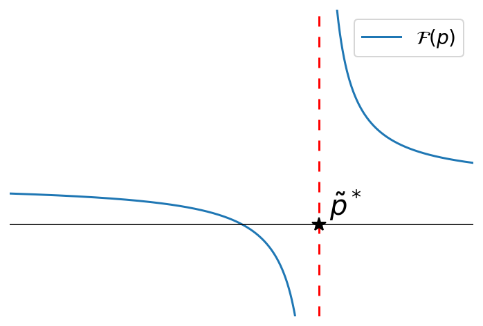
with $\mathcal{F}(p)=f(p)/\tilde{f}(p)$, where $f(p)=\alpha p+\beta$. The two possible forms of $\mathcal{F}(p)$ are shown in Figures 3(e)-(f) (Appendix C). An increase of $E[U|a)]$ ( i.e. $\Delta E[U|a]>0$) requires either a positive or a negative $\Delta k$, depending on the signs of $\tilde{f}(p_{k})$ and $(\mathcal{F}(p_{k})-\mathcal{F}(p_{j}))$. As $\tilde{f}(p)$ can take various shapes with respect to $f(p)$ (as shown in Figures 3(a)-(d)) there are several cases to consider.

A simple case is that the function $\tilde{f}(p)$ is strictly positive in $[0,1]$. Then, $\frac{\tilde{f}(p_{k})w_{k}}{\tilde{f}(p_{j})w_{j}}$ is positive, and $\tilde{f}(p_{k})\big(\mathcal{F}(p_{k})-\mathcal{F}(p_{j})\big)$ is positive (see $\mathcal{F}(p)$ in Figure 3(e) on the right side of the vertical asymptote). Thus, a positive $\Delta E[U|a]$ requires $\Delta_{k}>0$ (Eq. (8)) and $\Delta_{j}<0$ (Eq. (7)). This, in turn, requires that $d_{j}>0$ and $d_{k}<1$. It is easy to see that there exists at least one pair ($j,k$) with $d_{j}>0$ and $d_{k}<1$, unless the following condition holds: if $d_{j}>0$, then, for all $k>j$, $d_{k}=1$. This, however, characterizes a lower-bound threshold rule. Thus, unless $d$ represents a lower-bound threshold rule, one can construct a new rule with the same $E[V|a]$ and a higher $E[U|a]$.

The full proof in Appendix B leads through all possible cases. It shows that it is always possible to find a change $(\Delta_{j},\Delta_{k})$ fulfilling Equation (7) which leads to a positive $\Delta E[U|a]$, unless $d$ is a lower- or upper-bound threshold rule, which proves theorem 3.1 for any discretized approximation of calculating $E[U]$. Taking the limit $N\to\infty$ proves theorem 3.1 for the exact calculation of $E[U]$. The proofs for the conditional cases $E[V|J=j,a]$ with $J=Y$ and $J=D$ are given in Appendix D.

Theorem 3.1 has a restricted view on a single group $a$. In the following, we consider multiple groups and derive conditions for Pareto-optimal decision rules with respect to expected DM utility and fairness score.

First, we introduce the concept of Pareto optimality.

The set of all Pareto-optimal decision rules is defined as the Pareto frontier. The following optimality theorem specifies the Pareto-optimal solutions in the two-dimensional space $(E[U],FS)$.

Theorem 3.3 implies that, for a given population of individuals with feature vectors $\vec{x}$, there exists an upper bound on achievable DM utility for each level of fairness, as well as an upper bound on achievable fairness for each level of DM utility. No decision rule $\vec{x}\mapsto d(\vec{x})$ applied to the same population can exceed this theoretical boundary. Consequently, the resulting Pareto frontier defines the best utility-fairness tradeoff across all technical approaches used to construct the decision system (e.g. pre-, in-, or post-processing), and thus manifests a technology-agnostic benchmark.

Theorem 3.3 is widely applicable as it holds for arbitrary populations and group compositions, for any (reasonable) DM utility function and any (possibly group-specific) DS utility function, and for arbitrary scalar fairness scores calculated from $E[V|J=j,a]$ where $J\in\{D,Y,\emptyset\}$. It generalizes earlier results (Corbett-Davies et al., 2017; Baumann et al., 2022; Hardt et al., 2016) to fairness, freely specified DS utility functions that capture how decisions generate benefits or harms for individuals, and a wide range of fairness notions, including non-egalitarian ones.

The theorem states that, for any given group, the Pareto-optimal decision rule may be a lower-bound threshold rule (as in the seminal papers of 2016-17 (Corbett-Davies et al., 2017; Hardt et al., 2016)) but, under certain conditions, may equally well be an upper-bound threshold rule, i.e. $D=1$ for $p<t_{a}$, which is somewhat counter-intuitive, but has already been observed and discussed in recent works such as (Baumann et al., 2022; Favier and Calders, 2025).

Note that Theorem 3.3 is based on the assumption that the decision rules for different groups can be optimized independently. This seems to imply that the decision system needs access to the sensitive attribute $a$. However, this is not necessarily the case. While including $a$ in the feature vector $\vec{x}$ guarantees that group-specific decision rules can be implemented, and thus is a sufficient condition of fulfilling the prerequisites of Theorem 3.3, this is not a necessary condition. Consider a case where $\vec{x}$ does not contain $a$, but other features which are sufficiently correlated with $a$. Then, $a$ can be reconstructed from $\vec{x}$ (at least approximately), which allows implementing group-specific decision rules. An example is given in Section 5 where a trained decision algorithm does not use $a$ but still leads to group-specific thresholds as Pareto-optimal decision rules. We may conclude that any algorithm optimized for determining Pareto-optimal solutions can be expected to approximate the optimal solution given by Theorem 3.3, as far as its model structure allows.

Theorem 3.3 characterizes the Pareto-optimal decision rules, but does not fully specify the actual Pareto-optimal rules: while all Pareto-optimal solutions are group-dependent threshold rules, not all group-dependent threshold rules are Pareto-optimal. However, it is easy to see how the theorem leads to a simple constructive approach to determine the Pareto frontier. In a first step, all combinations of group-specific ub (upper-bound) and lb (lower-bound) threshold rules (with thresholds $t_{a}\in[0,1]$) are evaluated with respect to $E[U|a]$ and $E[V|J=j,a]$, for all groups $a\in A$, from which $E[U]$ and $FS$ can be determined. In a second step, the Pareto frontier is determined by identifying all non-Pareto-dominated combinations.

Furthermore, since $E[U]$ and $E[V|J=j,a]$ are continuous functions of the thresholds, the Pareto frontier can be approximated by limiting the evaluation of all threshold rules (which are infinitely many) to finite grid of thresholds in $[0,1]$. For the case of two groups, a grid of $M$ threshold values in $[0,1]$ for each group leads to $2M\times 2M$ decision rules, the non-dominated ones being Pareto-optimal solutions. The larger $M$ is, the more accurately the shape of the Pareto frontier is sampled.

The results in Section 3.3 are still theoretical, as they are based on the assumption that $p(\vec{x})$ is known. However, our framework suggest at least two different approaches of estimating the location of the Pareto frontier from empirical data.

The first approach is straight-forward: It consists in using machine learning methods for predicting $P[Y=1|\vec{x}]$, resulting in an estimate $\hat{p}(\vec{x})$ for all $\vec{x}$. For a test set of data samples $(\vec{x},Y,a)$, one can test different threshold combinations with both ub and lb threshold rules. This leads to estimates of $E[U]$ and $FS$. The resulting empirical Pareto frontier is an estimate of the true Pareto frontier. Stochastic variations are expected due to both the imperfection of the prediction model and the finiteness of the test set.

Note, however, that the location of the Pareto frontier can be determined even without using a predictor of $P[Y=1|\vec{x}]$ over the feature space. From Equations (3) and (4) we see that, for determining $E[U|a]$ and $E[V|J=j,a]$, we only need to know the distributions $g(p|a)$. Thus, a second approach is to estimate the distributions $g(p|a)$, and to use Equations (3) and (4) for evaluating different threshold rules (see Section 4 for an application of this approach). While $g(p|a)$ still needs to be determined from training data, it is arguably much easier to estimate this one-dimensional densities than to find a good predictor of $p(\vec{x})$ in a multi-dimensional feature space ⁹⁹9It is beyond the scope of this paper to discuss appropriate estimation methods. Note, however, that an important characteristic of $g(p|a)$ is the empirical base rate..