跳到论文正文
W Papers独立论文阅读器 arXiv:2605.08993 论文正文 计算阅读时间 · 0%
引用这篇论文根据当前论文元数据生成,正式投稿前建议核对。


License: arXiv.org perpetual non-exclusive license
arXiv:2605.08993v1 [nlin.CD] 09 May 2026

Reconstructing resonant phase oscillator interactions from noisy time series

Bengi Dönmez, Bob Rink Department of Mathematics, Vrije Universiteit Amsterdam, Amsterdam, the Netherlands, b.donmez@vu.nl Department of Mathematics, Vrije Universiteit Amsterdam, Amsterdam, the Netherlands, b.w.rink@vu.nl
(May 9, 2026)
Abstract

We present a novel method for reconstructing networks of coupled phase oscillators from noisy time series. Noise and uncertainty can make it hard or impossible to distinguish different oscillator networks based on observed dynamical behavior. Thus, our method does not aim to determine exact phase equations for the oscillators, but instead recovers their first and second order resonant normal form. This normal form contains crucial information on the underlying network and yields accurate approximations of the dynamics. We provide rigorous estimates on the accuracy of the reconstructed normal form, and we illustrate the method with numerical examples.

1 Introduction

Networks of coupled oscillators arise abundantly in physics, biology, and engineering, and they are often modeled by coupled differential equations. The goal of network reconstruction methods is to infer the coupling topology of such networks from observations of solutions to these differential equations. Many of these methods work by first extracting phase signals from oscillatory time series generated by the network, and subsequently fitting a phase vector field to these phase signals. Unfortunately, the resulting reconstructed phase equations typically do not allow us to infer the full coupling topology of the original network. One reason is that distinct oscillator networks may generate very similar dynamics, which may become indistinguishable when the observations of the systems are limited, noisy, or ill-conditioned. However, even in the absence of noise and uncertainty in the observations, the relation between the original oscillator network and the equations of motion for its phases is ambiguous, due to the intrinsic non-uniqueness of phase variables and phase extraction methods. As a result of this non-uniqueness, the same oscillator network may faithfully be described by multiple distinct phase equations, while the same phase equations may govern a variety of oscillator networks. This ambiguity forms a fundamental obstruction to the reliable reconstruction of an oscillator network from observations of its dynamics.

In this paper, we address this problem by presenting a new reconstruction method for networks of weakly coupled phase oscillators. Rather than attempting to reconstruct the exact equations of motion of such networks from observations, our method reconstructs their so-called resonant normal form. Networks with the same normal form generate nearly identical dynamics over long timescales, and are thus indistinguishable in the presence of noise or uncertainty. On the contrary, networks with different normal forms typically display quantitatively different dynamical behavior. This makes it more feasible to reconstruct the normal form than the true equations of motion, and it allows us to quantify the error in the reconstructed normal form. The normal form also provides reliable predictions of the long-term dynamics of the true network, and it encodes structural properties of the true network, such as symmetries.

Problem setting

Concretely, we consider interacting phase oscillator systems of the form

ϕ˙j=ωj+ε​Fj(1)​(ϕ)+ε2​Fj(2)​(ϕ)+ε3​Rj(3)​(ϕ,ε)​for​ 1≤j≤n,\displaystyle\dot{\phi}_{j}=\omega_{j}+\varepsilon F_{j}^{(1)}(\phi)+\varepsilon^{2}F_{j}^{(2)}(\phi)+\varepsilon^{3}R_{j}^{(3)}(\phi,\varepsilon)\ \mbox{for}\ 1\leq j\leq n\,, (1)

where ϕj∈𝕋:=ℝ/2​π​ℤ\phi_{j}\in\mathbb{T}:=\mathbb{R}/2\pi\mathbb{Z} is a phase variable, ε≥0\varepsilon\geq 0 is a small coupling parameter, and the Fj(l)F_{j}^{(l)} smooth interaction functions with Fourier expansions

Fj(l)​(ϕ)=∑k∈ℤnAj,k(l)​ei​⟨k,ϕ⟩​with​Aj,k(l)¯=Aj,−k(l).\displaystyle\ F_{j}^{(l)}(\phi)=\sum_{k\in\mathbb{Z}^{n}}A_{j,k}^{(l)}e^{i\langle k,\phi\rangle}\ \mbox{with}\ \overline{A_{j,k}^{(l)}}=A_{j,-k}^{(l)}. (2)

Our goal is to reconstruct (some of) the Fourier coefficients Aj,k(l)A_{j,k}^{(l)} from finite time observations Φ(m)​(t)\Phi^{(m)}(t) (with 1≤m≤M1\leq m\leq M and 0≤t≤T0\leq t\leq T) of true solutions ϕ(m)​(t)\phi^{(m)}(t) to (1). We assume that the uncertainty in these observations is small and bounded, that is,

|ϕj(m)​(t)−Φj(m)​(t)|≤Lj​ε​for all​ 1≤j≤n,1≤m≤M​and​ 0≤t≤T,|\phi^{(m)}_{j}(t)-\Phi^{(m)}_{j}(t)|\leq L_{j}\varepsilon\ \mbox{for all}\ 1\leq j\leq n,1\leq m\leq M\ \mbox{and}\ 0\leq t\leq T\,,

and for some uniform constants L1,…,Ln>0L_{1},\ldots,L_{n}>0. We will argue in Section 2 that this is the natural assumption to make when (1) describes the dynamics on an invariant torus (or “phase reduction”) of a higher-dimensional coupled oscillator system, and when the phase signals Φ(m)​(t)\Phi^{(m)}(t) are extracted from observations of these high-dimensional oscillators.

Network reconstruction methods often work by fitting a nonlinear phase vector field of the form (1) to the observations Φ(m)​(t)\Phi^{(m)}(t), for instance, in the form of a finite Fourier series

ϕ˙j≈ωj+ε​∑k∈𝒦A^j,k​ei​⟨k,ϕ⟩,\dot{\phi}_{j}\approx\omega_{j}+\varepsilon\sum_{k\in\mathcal{K}}\hat{A}_{j,k}e^{i\langle k,\phi\rangle}\,, (3)

with 𝒦⊂ℤn\mathcal{K}\subset\mathbb{Z}^{n} a (large) finite “library” of pre-selected Fourier labels. The simplest option is perhaps to choose the A^j,k\hat{A}_{j,k} to be minimizers of the sum of squares

B↦∑j=1M|Φ˙(m)​(0)−ωj−ε​∑k∈𝒦Bj,k​ei​⟨k,Φ(m)​(0)⟩|2.B\mapsto\sum_{j=1}^{M}\left|\dot{\Phi}^{(m)}(0)-\omega_{j}-\varepsilon\sum_{k\in\mathcal{K}}B_{j,k}e^{i\langle k,\Phi^{(m)}(0)\rangle}\right|^{2}\,. (4)

An alternative to fitting a phase vector field to observed phase velocities as described above, is to fit a time-TT map to the finite-time phase drifts Φ(m)​(T)−Φ(m)​(0)−ωj​T\Phi^{(m)}(T)-\Phi^{(m)}(0)-\omega_{j}T. This idea appears for instance in [14, 21], and it avoids the use of instantaneous phase velocities – which can be hard to determine accurately in practice. We present a related approach in this paper, which works by fitting “resonant” time-TT maps. Specifically, we present a first order and a second order resonant reconstruction method.

First order resonant reconstruction

Our first order method relies on Lemma 4.2 below, which states that, under mild conditions on (1) and (2), any exact solution to (1) satisfies

ϕj​(T)−ϕj​(0)−ωj​T=ε​T​∑⟨ω,k⟩=0Aj,k(1)​ei​⟨k,ϕ​(0)⟩+𝒪​(ε)​when​T∼1ε.\displaystyle\phi_{j}(T)\!-\!\phi_{j}(0)\!-\!\omega_{j}T=\varepsilon T\!\!\sum_{\langle\omega,k\rangle=0}\!\!A_{j,k}^{(1)}e^{i\langle k,\phi(0)\rangle}+\mathcal{O}(\varepsilon)\,\ \mbox{when}\ T\sim\frac{1}{\sqrt{\varepsilon}}. (5)

Thus, apart from a small correction of the order ε\varepsilon, over timescales of the order T∼1εT\sim\frac{1}{\sqrt{\varepsilon}}, every solution to (1) is governed by a slow linear drift of the order ε​T∼ε\varepsilon T\sim\sqrt{\varepsilon} away from the unperturbed motion ϕj​(T)=ϕj​(0)+ωj​T\phi_{j}(T)=\phi_{j}(0)+\omega_{j}T. It is important to remark that this linear phase drift is determined by so-called resonant terms only, that is, the terms Aj,k(1)​ei​⟨k,ϕ⟩A_{j,k}^{(1)}e^{i\langle k,\phi\rangle} in (2) with ⟨ω,k⟩=0\langle\omega,k\rangle=0. Nonresonant terms (those for which ⟨ω,k⟩≠0\langle\omega,k\rangle\neq 0) do not contribute to the linear phase drift. Their contribution to the dynamics is instead contained in the correction term of the order ε\varepsilon.

Inspired by this observation, our first order resonant reconstruction method first selects a finite library

𝒦⊂{k∈ℤn|⟨ω,k⟩=0}\mathcal{K}\subset\{k\in\mathbb{Z}^{n}\,|\,\langle\omega,k\rangle=0\}

of resonant Fourier labels, fixes a time TT of the order 1ε\frac{1}{\sqrt{\varepsilon}}, and then chooses the coefficients A^j,k\hat{A}_{j,k} in (3) to be minimizers of the sum of squares

B↦∑m=1M|Φj(m)​(T)−Φj(m)​(0)−ωj​T−ε​T​∑k∈𝒦Bj,k​ei​⟨k,Φ(m)​(0)⟩|2.B\mapsto\sum_{m=1}^{M}\left|\Phi_{j}^{(m)}(T)-\Phi_{j}^{(m)}(0)-\omega_{j}T-\varepsilon T\sum_{k\in\mathcal{K}}B_{j,k}e^{i\langle k,\Phi^{(m)}(0)\rangle}\right|^{2}\,.

This procedure yields estimates for the first order resonant Fourier coefficients in (1), and it does not attempt to estimate the nonresonant coefficients. The reason is that the contribution of the nonresonant terms to the dynamics is of the order ε\varepsilon. It is therefore of the same order of magnitude as the uncertainty in the observed phase drifts

|(Φj(m)​(T)−Φj(m)​(0)−ωj​T)−(ϕj(m)​(T)−ϕj(m)​(0)−ωj​T)|∼ε.|(\Phi_{j}^{(m)}(T)-\Phi_{j}^{(m)}(0)-\omega_{j}T)-(\phi_{j}^{(m)}(T)-\phi_{j}^{(m)}(0)-\omega_{j}T)|\sim\varepsilon\,.

The nonresonant Fourier coefficients in (2) therefore cannot realistically be inferred from the observations Φ(m)​(t)\Phi^{(m)}(t), and any attempt to estimate them would lead to an underdetermined or ill-conditioned regression problem. On the contrary, the estimators A^j,k\hat{A}_{j,k} provided by our resonant reconstruction method can often be guaranteed to lie close to the true first order resonant Fourier coefficients Aj,k(1)A_{j,k}^{(1)}. In particular, Theorem 5.1 roughly speaking states that

Aj,k(1)−A^j,k∼ε​for all​ 1≤j≤n​and​k∈𝒦,A^{(1)}_{j,k}-\hat{A}_{j,k}\sim\sqrt{\varepsilon}\ \mbox{for all}\ 1\leq j\leq n\ \mbox{and}\ k\in\mathcal{K}\,,

under certain verifiable conditions on the observations Φ(m)​(t)\Phi^{(m)}(t). The presence of bounded noise makes it impossible to derive similar rigorous bounds for estimators of nonresonant Fourier coefficients.

To illustrate the strength of our first order resonant reconstruction method, we refer to Figures 1, 2 and 3, in which we compare the performance of our resonant method with a reconstruction method that fits a time TT-map with both resonant and nonresonant terms to observations of finite time phase drifts. The figures show that resonant reconstruction is consistently reliable in the presence of observational noise, while the more general reconstruction method starts to fail as the noise level is increased.

Refer to caption
Figure 1: Comparison of resonant and nonresonant network reconstruction methods in the absence of observational noise. We consider a directed Erdős-Rényi graph with n=10n=10 nodes, where a directed edge probability p=15p=\frac{1}{5} was used to generate the graph. Phase dynamics is defined for each node of this graph by randomly choosing an intrinsic frequency ωi∈{1,2,3}\omega_{i}\in\{1,2,3\} for each node, fixing the coupling strength ε=0.01\varepsilon=0.01, and coupling the nodes by sinusoidal interaction functions of the form ε​ai​j​sin⁡(ϕi−ϕj)\varepsilon a_{ij}\sin(\phi_{i}-\phi_{j}), where ai​j∈{0,1}a_{ij}\in\{0,1\} are the coefficients of the adjacency matrix of the graph. The resulting phase dynamics was integrated using ode89 in Matlab over the time interval [0,T]=[0,ε−12]=[0,10][0,T]=[0,\varepsilon^{-\frac{1}{2}}]=[0,10] for a total of M=50M=50 initial conditions, chosen independently from the uniform distribution on [0,2​π]10[0,2\pi]^{10}. Time-TT maps were then fitted to the phase drifts observed in the resulting time series, using two different libraries: a resonant library containing the functions sin⁡(ϕi−ϕj)\sin(\phi_{i}-\phi_{j}) only when ωi=ωj\omega_{i}=\omega_{j} and i≠ji\neq j, and an all-pairs library containing sin⁡(ϕi−ϕj)\sin(\phi_{i}-\phi_{j}) for all i≠ji\neq j. From left to right: original network with ai​j∈{0,1}a_{ij}\in\{0,1\}; resonant subnetwork consisting of the connections in the original network with ωi=ωj\omega_{i}=\omega_{j}; reconstruction using the resonant library; reconstruction using the all-pairs library. In this noise-free setting, the all-pairs reconstruction provides an excellent approximation of the original network: the two networks are visually almost indistinguishable.
Refer to caption
Figure 2: Comparison of resonant and nonresonant network reconstruction methods with small observational noise. The original network is the same as in Figure 1 but the integrated time series were perturbed by i.i.d. random variables uniformly distributed on [−ε,ε][-\varepsilon,\varepsilon] (mean 0, variance ε2/3\varepsilon^{2}/3) before the reconstruction step. The resonant reconstruction remains a good approximation of the resonant subnetwork, whereas the all-pairs reconstruction already shows some discrepancies from the original network.
Refer to caption
Figure 3: Comparison of resonant and nonresonant network reconstruction methods with stronger observational noise. The original network is the same as in Figure 1 but the integrated time series were perturbed by i.i.d. random variables uniformly distributed on [−4​ε,4​ε][-4\varepsilon,4\varepsilon] (mean 0, variance 16​ε2/316\varepsilon^{2}/3) before the reconstruction step. In this case, the all-pairs reconstruction is quite different from the original network, while the resonant reconstruction still captures the resonant subnetwork in a robust way.

Second order resonant reconstruction

The second reconstruction method that we present can be used when (1) does not contain any first order resonant terms, that is, when Aj,k(1)=0A_{j,k}^{(1)}=0 if ⟨ω,k⟩=0\langle\omega,k\rangle=0. In this case, the first order resonant terms do not provide any information on the network topology. We will nevertheless show that

ϕj​(T)−ϕj​(0)−ωj​T=ε2​T​∑⟨ω,k⟩=0Cj,k(2)​ei​⟨k,ϕ​(0)⟩+𝒪​(ε)​when​T∼ε−32,\displaystyle\phi_{j}(T)\!-\!\phi_{j}(0)\!-\!\omega_{j}T=\varepsilon^{2}T\!\!\sum_{\langle\omega,k\rangle=0}\!\!C_{j,k}^{(2)}e^{i\langle k,\phi(0)\rangle}+\mathcal{O}(\varepsilon)\,\ \mbox{when}\ T\sim\varepsilon^{-\frac{3}{2}}\,,

where the Cj,k(2)C_{j,k}^{(2)} are the Fourier coefficients of the so-called second order resonant normal form of (1). It follows that, up to a small correction of the order ∼ε\sim\varepsilon, over timescales of the order T∼ε−32T\sim\varepsilon^{-\frac{3}{2}}, solutions to (1) are once more governed by a slow linear drift of the order ε2​T∼ε12\varepsilon^{2}T\sim\varepsilon^{\frac{1}{2}}. This drift is again determined only by resonant terms, while the impact of nonresonant terms is too small to be distinguished from observational noise. Similarly to the first order method described above, our second order resonant reconstruction method fits a resonant time-TT map to observations of phase drifts over a timescale T∼ε−32T\sim\varepsilon^{-\frac{3}{2}}, by computing least squares estimators C^j,k\hat{C}_{j,k} of the actual coefficients Cj,k(2)C_{j,k}^{(2)} of the second order normal form. We are also able to formulate verifiable conditions under which the reconstructed coefficients provide a reliable approximation of the true second order normal form coefficients, see Theorem 8.1, and we illustrate the method with a numerical example.

Discussion

A key challenge in data-driven model reconstruction is that the observations of the underlying dynamical system are often limited or noisy. This may lead to an ill-conditioned regression problem, overfitting, and non-uniqueness in the inferred dynamical equations. It is then common to select a reconstruction using statistical regularization, such as LASSO or Basis Pursuit. For example, the Sparse Identification of Nonlinear Dynamics (SINDy) method [4] in principle allows one to fit a large and possibly redundant function library (e.g., consisting of Fourier basis functions) to the observations, but selects a sparse reconstruction by penalizing for the number of nonzero basis functions that this reconstruction contains (e.g., the number of nonzero Fourier coefficients.) This method has been used successfully for reconstructing biological [13] and chemical [18] oscillator networks, and to explain observations of brain dynamics [6]. The Algorithm for Revealing Network Interactions (ARNI) [5] works in a similar manner. A related algorithm to stably reconstruct sparse networks from limited data was recently developed in [19, 20].

It was observed in [18] that SINDy sometimes automatically selects a resonant normal form as reconstruction of a coupled oscillator network. The authors of [18] explain this by showing that the normal form is often the sparsest ODE that generates the same dynamics as the true network up to a certain error margin. In this paper, we adopt a contrasting approach, by imposing in advance that our reconstruction consists only of resonant terms. We thereby guarantee the sparsity of the reconstruction a priori, which allows us to avoid statistical regularization altogether.

An obvious disadvantage of resonant reconstruction is that only some of the properties of a phase oscillator network are encoded in its normal form. These properties may not include all the strengths of all the couplings between the nodes in the network. For example, the first order normal form contains only the resonant first order interactions. The relation between a phase oscillator network and its second order normal form is much more intricate, as we show in Appendix D.

Organization of the paper

The remainder of this paper is organized as follows. In Section 2 we show why the assumption of bounded noise is natural in the context of reconstructing phase reductions. In Section 3 we present our first order reconstruction method. We prove the validity of this method in Sections 4 and 5 and investigate its performance through an example in Section 6. In Section 7 we present the second order reconstruction method. Its validity is proved in Section 8, and an application of the method is presented in Section 9. Several technical results on resonant normal forms are included in the appendices.

2 Phase reductions and bounded noise

Before presenting and analyzing our resonant reconstruction method in detail, we will first show in this section that small bounded uncertainties in the phase signals arise naturally when attempting to reconstruct phase equations for high-dimensional nonlinear oscillator systems. To see how phase equations are typically derived in this context, let us consider a network of weakly coupled differential equations of the form

x˙j=fj​(xj)+ε​gj​(x1,…,xn)​with​xj∈ℝdj​and​ 1≤j≤n,\dot{x}_{j}=f_{j}(x_{j})+\varepsilon g_{j}(x_{1},\ldots,x_{n})\ \mbox{with}\ x_{j}\in\mathbb{R}^{d_{j}}\ \mbox{and}\ 1\leq j\leq n\,, (6)

in which each ODE x˙j=fj​(xj)\dot{x}_{j}=f_{j}(x_{j}) in isolation possesses a stable limit cycle t↦γj​(t)t\mapsto\gamma_{j}(t) of minimal period TjT_{j} and frequency ωj:=2​π/Tj\omega_{j}:=2\pi/T_{j}. In the uncoupled situation (i.e., when ε=0\varepsilon=0), the product of these limit cycles defines an nn-dimensional normally hyperbolic invariant torus 𝐓(0)\mathbf{T}^{(0)} in the phase space ℝN\mathbb{R}^{N} (where N:=d1+…+dnN:=d_{1}+\ldots+d_{n}) of (6). One can assign to each point x∈𝐓(0)x\in\mathbf{T}^{(0)} a unique vector of phases

ϕ=(ϕ1,…,ϕn)∈𝕋n=(ℝ/2​π​ℤ)n\phi=(\phi_{1},\ldots,\phi_{n})\in\mathbb{T}^{n}=(\mathbb{R}/2\pi\mathbb{Z})^{n}

defined by the equality

x=E(0)​(ϕ):=(γ1​(ϕ1/ω1),…,γn​(ϕn/ωn))∈𝐓(0),x=E^{(0)}(\phi):=(\gamma_{1}(\phi_{1}/\omega_{1}),\ldots,\gamma_{n}(\phi_{n}/\omega_{n}))\in\mathbf{T}^{(0)}\,,

in terms of which the dynamics on the torus takes the form

ϕ˙j=ωj​for​ 1≤j≤n.\dot{\phi}_{j}=\omega_{j}\ \mbox{for}\ 1\leq j\leq n\,.

The flow on 𝐓(0)\mathbf{T}^{(0)} is thus quasi-periodic. Fénichel’s theorem [7] states that (6) will admit an invariant torus 𝐓(ε)\mathbf{T}^{(\varepsilon)} close to 𝐓(0)\mathbf{T}^{(0)} for small ε≠0\varepsilon\neq 0. Any parametrization E(ε):𝕋n→ℝNE^{(\varepsilon)}:\mathbb{T}^{n}\to\mathbb{R}^{N} of 𝐓(ε)\mathbf{T}^{(\varepsilon)} of the form

E(ε)​(ϕ)=E(0)​(ϕ)+ε​E(1)​(ϕ)+ε2​E(2)​(ϕ)+…E^{(\varepsilon)}(\phi)=E^{(0)}(\phi)+\varepsilon E^{(1)}(\phi)+\varepsilon^{2}E^{(2)}(\phi)+\ldots (7)

again associates a unique phase vector ϕ∈𝕋n\phi\in\mathbb{T}^{n} to each point x∈𝐓(ε)x\in\mathbf{T}^{(\varepsilon)}, and the ODEs governing their evolution are now of the form

ϕ˙j=ωj+ε​Fj(1)​(ϕ)+ε2​Fj(2)​(ϕ)+….\displaystyle\dot{\phi}_{j}=\omega_{j}+\varepsilon F_{j}^{(1)}(\phi)+\varepsilon^{2}F_{j}^{(2)}(\phi)+\ldots\,. (8)

Equation (8) is called a phase reduction of (6) and it describes the dynamics on 𝐓(ε)\mathbf{T}^{(\varepsilon)} in terms of the phase variables defined by (7). Phase reductions can be computed analytically from the original equations (6) by a variety of asymptotic methods, see for instance [3, 16, 22, 15, 1, 12, 17, 2, 11].

Because the persisting torus 𝐓(ε)\mathbf{T}^{(\varepsilon)} is (locally or globally) attracting, the solutions to (6) that are actually observed in numerical simulations or experiments will typically lie on or close to 𝐓(ε)\mathbf{T}^{(\varepsilon)}. As a result, data-driven reconstruction methods for coupled oscillator systems often aim to recover the phase equations (8) instead of the full equations (6). This is usually done by taking a collection of (possibly noisy) finite time observations X(m)​(t)∈ℝNX^{(m)}(t)\in\mathbb{R}^{N} (with 1≤m≤M1\leq m\leq M) of true solutions x(m)​(t)x^{(m)}(t) to (6) lying on or close to 𝐓(ε)\mathbf{T}^{(\varepsilon)}. Each signal X(m)​(t)X^{(m)}(t) is then transformed into a phase signal, i.e., a function Φ(m)​(t)∈ℝn\Phi^{(m)}(t)\in\mathbb{R}^{n} that satisfies

Φj(m)​(T)−Φj(m)​(0)=ωj​T+𝒪​(ε​T)​for​ 1≤j≤n.\Phi^{(m)}_{j}(T)-\Phi^{(m)}_{j}(0)=\omega_{j}T+\mathcal{O}(\varepsilon T)\ \mbox{for}\ 1\leq j\leq n. (9)

Such phase signals can be constructed in various ways, for instance by applying delayed embedding or a Hilbert transform to the X(m)​(t)X^{(m)}(t), often combined with a choice of filtering technique, see [14, 21, 9, 10]. The main idea is that the Φ(m)​(t)\Phi^{(m)}(t) will be approximations of lifts of true solutions ϕ(m)​(t)\phi^{(m)}(t) of a phase reduction (8) of (6). The final step of the reconstruction method consists of fitting a nonlinear phase vector field to the phase signals Φ(m)​(t)\Phi^{(m)}(t) as discussed in Section 1.

Limited, noisy or ill-conditioned observations X(m)​(t)X^{(m)}(t) may have a negative effect on the quality of the reconstruction (3) of (8). Moreover, even with perfect knowledge of the phase equations (8), it can be challenging to infer information about the original high-dimensional equations (6). One well-known problem is that the phase equations need not reflect the exact network topology of (6). Specifically, it was found in [18, 9, 10, 24, 23] that the phase equations (3) and (8) may display multi-body interactions, even when the original equations (6) are governed by two-body (“dyadic”) interactions only. In [9, 10, 23], these “virtual” or “emergent” multi-body interactions have been explained as a result of the phase reduction process, while in [18] they were interpreted as resonant terms in the normal form of the phase equations.

This paper is motivated by a more fundamental problem that complicates the interpretation of reconstructed phase equations, and which to our knowledge has not received attention in the literature on network reconstruction: the fact that phase reductions are not unique, because the choice of phase variables on the invariant torus 𝐓(ε)\mathbf{T}^{(\varepsilon)} is not unique, see [8]. This nonuniqueness means that the extracted phase signals Φ(m)​(t)\Phi^{(m)}(t) may not all be (approximations of) solutions of the same dynamical system.

To explain this, let us fix a choice of “reference” phase variables ϕ∈𝕋n\phi\in\mathbb{T}^{n}, defined by a reference embedding x=E(ε)​(ϕ)∈𝐓(ε)x=E^{(\varepsilon)}(\phi)\in\mathbf{T}^{(\varepsilon)}. The time-evolution of these phase variables is then governed by an ODE of the form (8). In view of equation (9), we can also assume that the observations Φ(m)​(t)\Phi^{(m)}(t) approximate the evolution of some phase variables, say

|ψj(m)​(t)−Φj(m)​(t)|≤Lj(1)​ε​for​ 1≤j≤n​and​ 1≤m≤M,\displaystyle|\psi^{(m)}_{j}(t)-\Phi^{(m)}_{j}(t)|\leq L_{j}^{(1)}\varepsilon\ \mbox{for}\ 1\leq j\leq n\ \mbox{and}\ 1\leq m\leq M\,, (10)

where the phases ψ∈𝕋n\psi\in\mathbb{T}^{n} are defined through some embedding x=E~(ε)​(ψ)x=\widetilde{E}^{(\varepsilon)}(\psi). However, it is not necessarily the case that E~(ε)=E(ε)\widetilde{E}^{(\varepsilon)}=E^{(\varepsilon)}, and the embedding E~(ε)\widetilde{E}^{(\varepsilon)} may even be different for each 1≤m≤M1\leq m\leq M. The ψ(m)​(t)\psi^{(m)}(t) may therefore not be solutions to the reference equations (12). Indeed, when E(ε)​(ϕ)=E(0)​(ϕ)+ε​E(1)​(ϕ)+ε2​…=E(0)​(ψ)+ε​E~(1)​(ψ)+ε2​…=E~(ε)​(ψ)E^{(\varepsilon)}(\phi)=E^{(0)}(\phi)\!+\!\varepsilon E^{(1)}(\phi)\!+\!\varepsilon^{2}\ldots\!=\!E^{(0)}(\psi)\!+\!\varepsilon\widetilde{E}^{(1)}(\psi)\!+\!\varepsilon^{2}\ldots=\widetilde{E}^{(\varepsilon)}(\psi) are two different embeddings of 𝐓(ε)\mathbf{T}^{(\varepsilon)}, then

ψ=H(ε)​(ϕ)=ϕ+ε​H(1)​(ϕ)+ε2​…\psi=H^{(\varepsilon)}(\phi)=\phi+\varepsilon H^{(1)}(\phi)+\varepsilon^{2}\ldots (11)

for some smooth change of coordinates H(ε):𝕋n→𝕋nH^{(\varepsilon)}:\mathbb{T}^{n}\to\mathbb{T}^{n}. Using that the equations of motion for the phases ϕ\phi are given by the interaction functions F(1),F(2),…F^{(1)},F^{(2)},\ldots as in (8), it follows that

ψ˙j=ωj+ε​(Fj(1)​(ψ)+∑k=1nωk​(∂kHj(1))​(ψ))+ε2​….\displaystyle\dot{\psi}_{j}=\omega_{j}+\varepsilon\left(F^{(1)}_{j}(\psi)+\sum_{k=1}^{n}\omega_{k}\left(\partial_{k}H^{(1)}_{j}\right)(\psi)\right)+\varepsilon^{2}\ldots\,. (12)

This confirms that the evolution of the phases ψ=(ψ1,…​ψn)\psi=(\psi_{1},\ldots\psi_{n}) is governed by interaction functions F~(1),F~(2),…\widetilde{F}^{(1)},\widetilde{F}^{(2)},\ldots that are generally different from those governing the evolution of the phases ϕ=(ϕ1,…,ϕn)\phi=(\phi_{1},\ldots,\phi_{n}). On the other hand, equation (11) implies that

|ψj(m)​(t)−ϕj(m)​(t)|≤Lj(2)​ε​for​ 1≤j≤n​and​ 1≤m≤M,\displaystyle|\psi^{(m)}_{j}(t)-\phi^{(m)}_{j}(t)|\leq L_{j}^{(2)}\varepsilon\ \mbox{for}\ 1\leq j\leq n\ \mbox{and}\ 1\leq m\leq M\,, (13)

for some uniform constant Lj(2)>0L_{j}^{(2)}>0. Together (10) and (13) imply that

|ϕj(m)​(t)−Φj(m)​(t)|≤|ϕj(m)​(t)−ψj(m)​(t)|+|ψj(m)​(t)−Φj(m)​(t)|≤Lj​ε,|\phi^{(m)}_{j}(t)-\Phi^{(m)}_{j}(t)|\leq|\phi^{(m)}_{j}(t)-\psi^{(m)}_{j}(t)|+|\psi^{(m)}_{j}(t)-\Phi^{(m)}_{j}(t)|\leq L_{j}\varepsilon\,,

where Lj:=Lj(1)+Lj(2)L_{j}:=L_{j}^{(1)}+L_{j}^{(2)}. The term |ψj(m)​(t)−Φj(m)​(t)||\psi^{(m)}_{j}(t)-\Phi^{(m)}_{j}(t)| in this expression can be thought of as observational noise (which may even vanish when the observations are perfect.) The term |ϕj(m)​(t)−ψj(m)​(t)||\phi^{(m)}_{j}(t)-\psi^{(m)}_{j}(t)| reflects the intrinsic mismatch between reference phases and observed phases.

In practice, it may be hard to distinguish these two sources of uncertainty in the phase signals. We therefore do not make this distinction in this paper, by simply assuming that |ϕj(m)​(t)−Φj(m)​(t)|≤Lj​ε|\phi^{(m)}_{j}(t)-\Phi^{(m)}_{j}(t)|\leq L_{j}\varepsilon for a uniform constant LjL_{j}.

3 First order resonant reconstruction

We now present the details of our first order resonant reconstruction method for equations of the form (1). Our method relies on the assumption that we are given reasonable estimates of the coupling strength ε\varepsilon and the oscillator frequencies ω1,…,ωn\omega_{1},\ldots,\omega_{n} in (1) from the start.

Remark 3.1.

For a fixed value of ε≠0\varepsilon\neq 0, the constant Fourier-term (i.e., the sum of the ϕ\phi-independent terms) in equation (1) is

Ωj=ωj+ε​Aj,0(1)+ε2​Aj,0(2)+𝒪​(ε3).\Omega_{j}=\omega_{j}+\varepsilon A_{j,0}^{(1)}+\varepsilon^{2}A_{j,0}^{(2)}+\mathcal{O}(\varepsilon^{3})\,.

This means that the frequency ωj\omega_{j} is only defined up to a term of the order ∼ε\sim\varepsilon. It may in fact be easier to estimate Ωj\Omega_{j} from observations than ωj\omega_{j}. We shall thus assume that we know the value of ωj\omega_{j} up to an error of the order ∼ε\sim\varepsilon. We simply include the unknown part of ωj\omega_{j} as unknown constant terms ε​Aj,0(1),ε2​Aj,0(2),…\varepsilon A_{j,0}^{(1)},\varepsilon^{2}A_{j,0}^{(2)},\ldots in (1). Our reconstruction method can estimate these terms. Similarly, the Fourier-coefficient of the term ei​⟨k,ϕ⟩e^{i\langle k,\phi\rangle} in (1) is

αj,k:=ε​Aj,k(1)+ε2​Aj,k(2)+𝒪​(ε3).\alpha_{j,k}:=\varepsilon A_{j,k}^{(1)}+\varepsilon^{2}A_{j,k}^{(2)}+\mathcal{O}(\varepsilon^{3})\,.

This means the values of the coupling strength ε\varepsilon and the coupling constants Aj,k(1),Aj,k(2),…A_{j,k}^{(1)},A_{j,k}^{(2)},\ldots are not unique: only their orders of magnitude are well-defined. It suffices to fix a value of ε\varepsilon such that Aj,k(1),Aj,k(2),…∼1A_{j,k}^{(1)},A_{j,k}^{(2)},\ldots\sim 1.

Our method for reconstructing equations (1) furthermore assumes that we are given noisy phase signals

Φ(m)​(t)∈ℝn​with​ 1≤m≤M.\Phi^{(m)}(t)\in\mathbb{R}^{n}\ \mbox{with}\ 1\leq m\leq M\,.

In fact, we only need to know the value of these phase signals at times

t=0​and​t=T:=1ε.t=0\ \mbox{and}\ t=T:=\frac{1}{\sqrt{\varepsilon}}\,.

As discussed above, we assume the noise in these phase signals to be small and bounded. More precisely, we will assume that there are constants Lj>0L_{j}>0 such that for every 1≤m≤M1\leq m\leq M, there is a (lift of an) exact solution ϕ(m)​(t)∈ℝn\phi^{(m)}(t)\in\mathbb{R}^{n} to (1) so that

|ϕj(m)​(0)−Φj(m)​(0)|≤Lj​ε​and​|ϕj(m)​(T)−Φj(m)​(T)|≤Lj​ε.|\phi^{(m)}_{j}(0)-\Phi^{(m)}_{j}(0)|\leq L_{j}\varepsilon\ \mbox{and}\ |\phi^{(m)}_{j}(T)-\Phi^{(m)}_{j}(T)|\leq L_{j}\varepsilon\,. (14)

Our first order reconstruction method can now be summarized as follows:

  1. 1)

    Fix an oscillator 1≤j≤n1\leq j\leq n and calculate the rescaled observed drifts

    Δ(m):=Φj(m)​(T)−Φj(m)​(0)−ωj​Tε​T∈ℝfor​ 1≤m≤M.{\Delta}^{(m)}:=\frac{\Phi^{(m)}_{j}(T)-\Phi^{(m)}_{j}(0)-\omega_{j}T}{\varepsilon T}\in\mathbb{R}\ \ \mbox{for}\ 1\leq m\leq M\,.

    These drifts together form a (column) vector Δ∈ℝM\Delta\in\mathbb{R}^{M}.

  2. 2)

    Select a finite library of resonant Fourier labels

    𝒦={k1,…,kK}⊂{k∈ℤn|⟨k,ω⟩=0},\mathcal{K}=\{k_{1},\ldots,k_{K}\}\subset\{k\in\mathbb{Z}^{n}\,|\,\langle k,\omega\rangle=0\}\,,

    where K:=|𝒦|K:=|\mathcal{K}|, and evaluate the functions ei​⟨k,ϕ⟩e^{i\langle k,\phi\rangle} (k∈𝒦k\in\mathcal{K}) at the observed initial states Φ(m)​(0)\Phi^{(m)}(0), to create the library matrix

    Θ:=(ei​⟨k1,Φ(1)​(0)⟩…ei​⟨kK,Φ(1)​(0)⟩⋮⋱⋮ei​⟨k1,Φ(M)​(0)⟩…ei​⟨kK,Φ(M)​(0)⟩):ℂK→ℂM.\Theta:=\left(\begin{array}[]{ccc}e^{i\langle k_{1},\Phi^{(1)}(0)\rangle}&\ldots&e^{i\langle k_{K},\Phi^{(1)}(0)\rangle}\\ \vdots&\ddots&\vdots\\ e^{i\langle k_{1},\Phi^{(M)}(0)\rangle}&\ldots&e^{i\langle k_{K},\Phi^{(M)}(0)\rangle}\end{array}\right):\mathbb{C}^{K}\to\mathbb{C}^{M}\,.

    We assume that the observations Φ(m)​(0)\Phi^{(m)}(0) (with m=1,…,Mm=1,\ldots,M) are sufficiently well spread over 𝕋n\mathbb{T}^{n} that Θ\Theta is injective.

  3. 3)

    List the resonant Fourier coefficients Aj,k(1)A_{j,k}^{(1)} (with k∈𝒦k\in\mathcal{K}) in the vector

    Aj(1):=(Aj,k1(1),…,Aj,kK(1))T∈ℂK.A_{j}^{(1)}:=(A^{(1)}_{j,k_{1}},\ldots,A^{(1)}_{j,k_{K}})^{T}\in\mathbb{C}^{K}\,.

    Inspired by (5), we estimate this vector by the vector

    A^j=(A^j,k1,…,A^j,kK)T∈ℂK\hat{A}_{j}=(\hat{A}_{j,k_{1}},\ldots,\hat{A}_{j,k_{K}})^{T}\in\mathbb{C}^{K}

    defined by

    A^j=arg⁡minB∈ℂK​∑m=1M|Δ(m)−∑i=1KBki​ei​⟨ki,Φ(m)​(0)⟩|2∈ℂK.\hat{A}_{j}={\arg\min}_{B\in\mathbb{C}^{K}}\sum_{m=1}^{M}\left|\Delta^{(m)}-\sum_{i=1}^{K}B_{k_{i}}e^{i\langle k_{i},\Phi^{(m)}(0)\rangle}\right|^{2}\in\mathbb{C}^{K}\,.

    It is well-known that this minimizer is unique when Θ\Theta is injective, and given by

    A^j=Θ+​(Δ)∈ℂK,\hat{A}_{j}=\Theta^{+}(\Delta)\in\mathbb{C}^{K}\,, (15)

    where Θ+:=(ΘH​Θ)−1​ΘH\Theta^{+}:=(\Theta^{H}\Theta)^{-1}\Theta^{H} is the Moore-Penrose pseudo-inverse of Θ\Theta and ΘH:=Θ¯T\Theta^{H}:=\overline{\Theta}^{T} its Hermitian transpose. We prove (15) in Appendix A for completeness.

This reconstruction method was used to generate Figures 1, 2 and 3 in the introduction. In the upcoming sections we will rigorously prove that the A^j,k\hat{A}_{j,k} are good estimators of the Aj,k(1)A_{j,k}^{(1)}, when certain natural conditions are satisfied. We give an application of the method in Section 6

4 Approximating the drift dynamics

The proof that the A^j,k\hat{A}_{j,k} are close to the true Fourier coefficients Aj,k(1)A_{j,k}^{(1)} hinges on Lemma 4.2 which implies that, to leading order, the flow of (1) is governed by first order resonant terms only. To show this, we first prove Lemma 4.1 by exploiting a combination of Picard iteration and Taylor expansion. By Ck​(𝕋n)C^{k}(\mathbb{T}^{n}) we denote the space of real-valued CkC^{k}-functions on 𝕋n\mathbb{T}^{n} and for an f∈C0​(𝕋n)f\in C^{0}(\mathbb{T}^{n}) we shall write

‖f‖0:=supϕ∈𝕋n|f​(ϕ)|.\|f\|_{0}:=\sup_{\phi\in\mathbb{T}^{n}}|f(\phi)|\,.

For a continuous function g:𝕋n×[−ε0,ε0]→ℝg:\mathbb{T}^{n}\times[-\varepsilon_{0},\varepsilon_{0}]\to\mathbb{R} we similarly denote ‖g‖0:=sup(ϕ,ε)∈𝕋n×[−ε0,ε0]|g​(ϕ,ε)|\|g\|_{0}:=\sup_{(\phi,\varepsilon)\in\mathbb{T}^{n}\times[-\varepsilon_{0},\varepsilon_{0}]}|g(\phi,\varepsilon)|.

Lemma 4.1.

For all 1≤j≤n1\leq j\leq n, assume that Fj(1)∈C1​(𝕋n)F^{(1)}_{j}\in C^{1}(\mathbb{T}^{n}) and Rj(2)∈C0​(𝕋n×[−ε0,ε0])R^{(2)}_{j}\in C^{0}(\mathbb{T}^{n}\times[-\varepsilon_{0},\varepsilon_{0}]). Let |ε|≤ε0|\varepsilon|\leq\varepsilon_{0} and let ϕ​(t)\phi(t) be a solution to

ϕ˙j=ωj+ε​Fj(1)​(ϕ)+ε2​Rj(2)​(ϕ,ε)​for all​ 1≤j≤n.\dot{\phi}_{j}=\omega_{j}+\varepsilon F_{j}^{(1)}(\phi)+\varepsilon^{2}R_{j}^{(2)}(\phi,\varepsilon)\ \mbox{for all}\ 1\leq j\leq n\,. (16)

Then

ϕj​(T)−ϕj​(0)−ωj​T=ε​∫0TFj(1)​(ϕ​(0)+ω​t)​𝑑t+rj(2)​(T,ε),\phi_{j}(T)-\phi_{j}(0)-\omega_{j}T=\varepsilon\int_{0}^{T}F^{(1)}_{j}(\phi(0)+\omega t)\,dt+r_{j}^{(2)}(T,\varepsilon)\,, (17)

in which

|rj(2)​(T,ε)|≤Aj​ε2​T2+Bj​ε2​T,|r_{j}^{(2)}(T,\varepsilon)|\leq A_{j}\varepsilon^{2}T^{2}+B_{j}\varepsilon^{2}T\,,

for constants Aj,BjA_{j},B_{j} independent of TT and ε\varepsilon, given in (24) and (26).

Proof.

Let us write Ri(1)​(ϕ,ε):=Fi(1)​(ϕ)+ε​Ri(2)​(ϕ,ε)R_{i}^{(1)}(\phi,\varepsilon):=F_{i}^{(1)}(\phi)+\varepsilon R_{i}^{(2)}(\phi,\varepsilon). Then Ri(1)R_{i}^{(1)} is a bounded continuous function on 𝕋n×[−ε0,ε0]\mathbb{T}^{n}\times[-\varepsilon_{0},\varepsilon_{0}], and ϕ˙i​(s)=ωi+ε​Ri(1)​(ϕ​(s),ε)\dot{\phi}_{i}(s)=\omega_{i}+\varepsilon R_{i}^{(1)}(\phi(s),\varepsilon) for all 1≤i≤n1\leq i\leq n. Integrating this equation from s=0s=0 to s=ts=t yields

ϕi​(t)=ϕi​(0)+ωi​t+ε​∫0tRi(1)​(ϕ​(s),ε)​𝑑s.\phi_{i}(t)=\phi_{i}(0)+\omega_{i}t+\varepsilon\int_{0}^{t}R^{(1)}_{i}(\phi(s),\varepsilon)\,ds\,. (18)

We see in particular that

ϕi​(t)=ϕi​(0)+ωi​t+ri(1)​(t,ε)in which|ri(1)​(t,ε)|≤|ε​t|​‖Ri(1)‖0.\phi_{i}(t)=\phi_{i}(0)+\omega_{i}t+r_{i}^{(1)}(t,\varepsilon)\ \ \mbox{in which}\ \ |r_{i}^{(1)}(t,\varepsilon)|\leq|\varepsilon t|\|R_{i}^{(1)}\|_{0}\,. (19)

Next, we integrate the equation ϕ˙j​(t)=ωj+ε​Fj(1)​(ϕ​(t))+ε2​Rj(2)​(ϕ​(t),ε)\dot{\phi}_{j}(t)=\omega_{j}+\varepsilon F_{j}^{(1)}(\phi(t))+\varepsilon^{2}R_{j}^{(2)}(\phi(t),\varepsilon) from t=0t=0 to t=Tt=T to find that

ϕj​(T)=ϕj​(0)+ωj​T+ε​∫0TFj(1)​(ϕ​(t))​𝑑t+ε2​∫0TRj(2)​(ϕ​(t),ε)​𝑑t.\displaystyle\phi_{j}(T)=\phi_{j}(0)+\omega_{j}T+\varepsilon\int_{0}^{T}F^{(1)}_{j}\left(\phi(t)\right)dt+\varepsilon^{2}\int_{0}^{T}\!R^{(2)}_{j}(\phi(t),\varepsilon)\,dt. (20)

To rewrite the first integral term, we use (19) to obtain

Fj(1)​(ϕ​(t))=Fj(1)​(ϕ​(0)+ω​t+r(1)​(t,ε))=Fj(1)​(ϕ​(0)+ω​t)+hj​(t,ε)F_{j}^{(1)}\left(\phi(t)\right)=F^{(1)}_{j}\left(\phi(0)+\omega t+r^{(1)}(t,\varepsilon)\right)=F^{(1)}_{j}\left(\phi(0)+\omega t\right)+h_{j}(t,\varepsilon) (21)

in which, in view of (19),

|hj​(t,ε)|≤∑i=1n‖∂iFj(1)‖0​|ri(1)​(t,ε)|≤|ε​t|​∑i=1n‖∂iFj(1)‖0​‖Ri(1)‖0.|h_{j}(t,\varepsilon)|\leq\sum_{i=1}^{n}\|\partial_{i}F^{(1)}_{j}\|_{0}|r_{i}^{(1)}(t,\varepsilon)|\leq|\varepsilon t|\sum_{i=1}^{n}\|\partial_{i}F^{(1)}_{j}\|_{0}\|R^{(1)}_{i}\|_{0}\,. (22)

Integration of (21) from t=0t=0 to t=Tt=T therefore gives

|ε​∫0TFj(1)​(ϕ​(t))​𝑑t−ε​∫0TFj(1)​(ϕ​(0)+ω​t)​𝑑t|≤ε​∫0T|hj​(t,ε)|​𝑑t≤Aj​ε2​T2\displaystyle\left|\varepsilon\!\int_{0}^{T}\!\!F^{(1)}_{j}\left(\phi(t)\right)\,dt-\varepsilon\!\int_{0}^{T}\!\!F^{(1)}_{j}\left(\phi(0)+\omega t\right)\,dt\right|\leq\varepsilon\int_{0}^{T}\!\!|h_{j}(t,\varepsilon)|\,dt\leq A_{j}\varepsilon^{2}T^{2} (23)

for the constant

Aj:=12​∑i=1n‖∂iFj(1)‖0​‖Ri(1)‖0.\displaystyle A_{j}:=\frac{1}{2}\sum_{i=1}^{n}\|\partial_{i}F^{(1)}_{j}\|_{0}\|R^{(1)}_{i}\|_{0}\,. (24)

The second term in (20) can clearly be bounded by

|ε2​∫0TRj(2)​(ϕ​(t),ε)​𝑑t|≤Bj​ε2​T\left|\varepsilon^{2}\int_{0}^{T}R^{(2)}_{j}(\phi(t),\varepsilon)\,dt\right|\leq B_{j}\varepsilon^{2}T (25)

for

Bj:=‖Rj(2)‖0.B_{j}:=\|R_{j}^{(2)}\|_{0}\,. (26)

Together, (20), (23) and (25) prove the Lemma. ∎

We now investigate why and in which exact sense Lemma 4.1 implies formula (5). Recall from (17) that the drift ϕj​(T)−ϕj​(0)−ωj​T\phi_{j}(T)-\phi_{j}(0)-\omega_{j}T of a solution to (1) can be approximated by the integral

ε​∫0TFj(1)​(ϕ​(0)+ω​t)​𝑑t\displaystyle\varepsilon\int_{0}^{T}F_{j}^{(1)}(\phi(0)+\omega t)\,dt (27)

of ε​Fj(1)\varepsilon F_{j}^{(1)} over the unperturbed flow t↦ϕ​(0)+ω​tt\mapsto\phi(0)+\omega t. One can expect that this integral is of the order ε​T\varepsilon T, and in particular that it is of the order ε\sqrt{\varepsilon} when TT is of the order 1ε\frac{1}{\sqrt{\varepsilon}}. On the other hand, Lemma 4.1 implies that the difference rj(2)​(T,ε)r_{j}^{(2)}(T,\varepsilon) between the true drift and (27) is of the order ε\varepsilon for T∼1εT\sim\frac{1}{\sqrt{\varepsilon}}. This means that, to leading order in ε\varepsilon and over timescales of the order 1ε\frac{1}{\sqrt{\varepsilon}}, the drift is determined by the integral (27).

We now analyze (27) in detail by splitting Fj(1)F^{(1)}_{j} into a library part, a remaining resonant part and a nonresonant part, by writing

Fj(1)​(ϕ)=Fj𝒦​(ϕ)+Fjℛ​(ϕ)+Fj𝒩​(ϕ),F_{j}^{(1)}(\phi)=F_{j}^{\mathcal{K}}(\phi)+F_{j}^{\mathcal{R}}(\phi)+F_{j}^{\mathcal{N}}(\phi)\,,

where

Fj𝒦​(ϕ)\displaystyle F_{j}^{\mathcal{K}}(\phi) =∑k∈𝒦Aj,k(1)​ei​⟨k,ϕ⟩,\displaystyle=\sum_{k\in\mathcal{K}}A_{j,k}^{(1)}e^{i\langle k,\phi\rangle}\,, (28)
Fjℛ​(ϕ)\displaystyle F_{j}^{\mathcal{R}}(\phi) =∑⟨k,ω⟩=0,k∉𝒦Aj,k(1)​ei​⟨k,ϕ⟩,\displaystyle=\sum_{\langle k,\omega\rangle=0,\,k\notin\mathcal{K}}A_{j,k}^{(1)}e^{i\langle k,\phi\rangle}\,, (29)
Fj𝒩​(ϕ)\displaystyle F_{j}^{\mathcal{N}}(\phi) =∑⟨k,ω⟩≠0Aj,k(1)​ei​⟨k,ϕ⟩.\displaystyle=\sum_{\langle k,\omega\rangle\neq 0}A_{j,k}^{(1)}e^{i\langle k,\phi\rangle}\,. (30)

Here, 𝒦⊂{k∈ℤn∣⟨ω,k⟩=0}\mathcal{K}\subset\left\{k\in\mathbb{Z}^{n}\mid\langle\omega,k\rangle=0\right\} is a finite library of resonant Fourier labels. We integrate these functions separately.

Library part (28): Because 𝒦\mathcal{K} is finite and ⟨k,ϕ​(0)+ω​t⟩=⟨k,ϕ​(0)⟩\langle k,\phi(0)+\omega t\rangle=\langle k,\phi(0)\rangle when kk is resonant, it is clear that

ε​∫0TFj𝒦​(ϕ​(0)+ω​t)​𝑑t=ε​∑k∈𝒦Aj,k(1)​∫0Tei​⟨k,ϕ​(0)+ω​t⟩​𝑑t=ε​T​∑k∈𝒦Aj,k(1)​ei​⟨k,ϕ​(0)⟩.\displaystyle\varepsilon\!\int_{0}^{T}\!\!F_{j}^{\mathcal{K}}(\phi(0)+\omega t)\,dt=\varepsilon\sum_{k\in\mathcal{K}}A_{j,k}^{(1)}\int_{0}^{T}\!\!e^{i\langle k,\phi(0)+\omega t\rangle}\,dt=\varepsilon T\sum_{k\in\mathcal{K}}A_{j,k}^{(1)}e^{i\langle k,\phi(0)\rangle}\,. (31)

Thus, the value of this integral increases slowly and linearly in TT, as was anticipated in formula (5). Note that over timescales of the order T∼1εT\sim\frac{1}{\sqrt{\varepsilon}}, the right hand side of (31) will typically be of the order ε\sqrt{\varepsilon}.

Remaining resonant part (29): Note that FjℛF_{j}^{\mathcal{R}} may potentially have an infinite Fourier series. We can nevertheless formally compute the integral of (29) term-by-term. This yields

ε​∫0TFjℛ​(ϕ​(0)+ω​t)​𝑑t\displaystyle\varepsilon\int_{0}^{T}F_{j}^{\mathcal{R}}(\phi(0)+\omega t)\,dt ∼ε​T​∑⟨k,ω⟩=0,k∉𝒦Aj,k(1)​ei​⟨k,ϕ​(0)⟩.\displaystyle\sim\varepsilon T\sum_{\langle k,\omega\rangle=0,\,k\notin\mathcal{K}}A_{j,k}^{(1)}e^{i\langle k,\phi(0)\rangle}\,. (32)

We would like this integral to converge and to be at most of the order ε\varepsilon on a timescale of the order T∼1εT\sim\frac{1}{\sqrt{\varepsilon}}. This can be ensured by requiring, for example, that

∑⟨k,ω⟩=0,k∉𝒦|Aj,k(1)|≤Cj​ε,\displaystyle\sum_{\langle k,\omega\rangle=0,\,k\notin\mathcal{K}}|A_{j,k}^{(1)}|\leq C_{j}\sqrt{\varepsilon}\,, (33)

meaning that the library is large enough to describe the most relevant resonant terms in Fj(1)F_{j}^{(1)}. Under condition (33), equation (32) becomes an equality, and we have

|ε​∫0TFjℛ​(ϕ​(0)+ω​t)​𝑑t|\displaystyle\left|\varepsilon\int_{0}^{T}F_{j}^{\mathcal{R}}(\phi(0)+\omega t)\,dt\right| ≤Cj​ε32​T.\displaystyle\leq C_{j}\varepsilon^{\frac{3}{2}}T\,. (34)

Note that the right hand side of (34) is of the order ε\varepsilon when T∼1εT\sim\frac{1}{\sqrt{\varepsilon}}. It is thus of the order of the error term rj(2)​(T,ε)r_{j}^{(2)}(T,\varepsilon) in (17) and considerably smaller than the right hand side of (31).

Nonresonant part (30): The nonresonant part Fj𝒩F_{j}^{\mathcal{N}} may similarly have an infinite Fourier series, so that its integral can only formally be computed to be

ε​∫0T\displaystyle\varepsilon\int_{0}^{T} Fj𝒩​(ϕ​(0)+ω​t)​d​t∼ε​∑⟨k,ω⟩≠0Aj,k(1)​∫0Tei​⟨k,ϕ​(0)+ω​t⟩​𝑑t\displaystyle F_{j}^{\mathcal{N}}(\phi(0)+\omega t)\,dt\sim\varepsilon\sum_{\langle k,\omega\rangle\neq 0}A_{j,k}^{(1)}\int_{0}^{T}e^{i\langle k,\phi(0)+\omega t\rangle}\,dt
=ε​∑⟨k,ω⟩≠0Aj,k(1)​ei​⟨k,ϕ​(0)⟩i​⟨k,ω⟩​(ei​⟨k,ω⟩​T−1).\displaystyle=\varepsilon\sum_{\langle k,\omega\rangle\neq 0}\frac{A_{j,k}^{(1)}e^{i\langle k,\phi(0)\rangle}}{i\langle k,\omega\rangle}\left(e^{i\langle k,\omega\rangle T}-1\right)\,. (35)

Each term in this formal sum is an oscillatory and uniformly bounded function of TT. We would like the sum to be bounded itself and of the order ε\varepsilon. This can be ensured by asking, for example, that

∑⟨k,ω⟩≠0|Aj,k(1)⟨k,ω⟩|≤12​Dj.\displaystyle\sum_{\langle k,\omega\rangle\neq 0}\left|\frac{A_{j,k}^{(1)}}{\langle k,\omega\rangle}\right|\leq\frac{1}{2}D_{j}\,. (36)

Under condition (36), equation (4) becomes an equality, and

|ε​∫0TFj𝒩​(ϕ​(0)+ω​t)​𝑑t|≤Dj​ε.\displaystyle\left|\varepsilon\int_{0}^{T}F_{j}^{\mathcal{N}}(\phi(0)+\omega t)\,dt\right|\leq D_{j}\varepsilon\,. (37)

Being of the order ε\varepsilon (uniformly in time), this integral is of the order of the error term rj(2)r_{j}^{(2)} in (17) and considerably smaller than the right hand side of (31) on the timescale T∼1εT\sim\frac{1}{\sqrt{\varepsilon}}.

The following result follows almost immediately from the discussion above:

Lemma 4.2.

Let 0≤ε≤ε00\leq\varepsilon\leq\varepsilon_{0} be given, and let 𝒦⊂{k∈ℤn|⟨k,ω⟩=0}\mathcal{K}\subset\{k\in\mathbb{Z}^{n}\,|\,\langle k,\omega\rangle=0\,\} be a finite set of resonant Fourier labels. Let us decompose

Fj(1)=Fj𝒦+Fjℛ+Fj𝒩,F^{(1)}_{j}=F_{j}^{\mathcal{K}}+F_{j}^{\mathcal{R}}+F_{j}^{\mathcal{N}}\,,

as defined in (28), (29) and (30). Let the assumptions of Lemma 4.1 be satisfied and assume in addition that for all ϕ∈𝕋n\phi\in\mathbb{T}^{n},

|∫0TFjℛ​(ϕ+ω​t)​𝑑t|≤Cj​ε​T​and​|∫0TFj𝒩​(ϕ+ω​t)​𝑑t|≤Dj\left|\int_{0}^{T}F_{j}^{\mathcal{R}}(\phi+\omega t)\,dt\right|\leq C_{j}\sqrt{\varepsilon}T\ \mbox{and}\ \left|\int_{0}^{T}F_{j}^{\mathcal{N}}(\phi+\omega t)\,dt\right|\leq D_{j}

for some constants Cj,DjC_{j},D_{j} independent of TT and ε\varepsilon. Then any solution t↦ϕ​(t)t\mapsto\phi(t) to (16) satisfies

ϕj​(T)−ϕj​(0)−ωj​T=ε​T​∑k∈𝒦Aj,k(1)​ei​⟨k,ϕ​(0)⟩+ρj(2)​(T,ε),\phi_{j}(T)-\phi_{j}(0)-\omega_{j}T=\varepsilon T\sum_{k\in\mathcal{K}}A_{j,k}^{(1)}e^{i\langle k,\phi(0)\rangle}+\rho_{j}^{(2)}(T,\varepsilon)\,,

in which

|ρj(2)​(T,ε)|≤Aj​ε2​T2+Bj​ε2​T+Cj​ε32​T+Dj​ε,\left|\rho_{j}^{(2)}(T,\varepsilon)\right|\leq A_{j}\varepsilon^{2}T^{2}+B_{j}\varepsilon^{2}T+C_{j}\varepsilon^{\frac{3}{2}}T+D_{j}\varepsilon\,,

and where the constants Aj,BjA_{j},B_{j} are given in (24) and (26).

Proof.

The proof was essentially given in the discussion above. Note that Lemma 4.1 states that

ϕj​(T)−ϕj​(0)−ωj​T=ε​∫0TFj(1)​(ϕ​(0)+ω​t)​𝑑t+rj(2)​(T,ε)\phi_{j}(T)-\phi_{j}(0)-\omega_{j}T=\varepsilon\int_{0}^{T}F_{j}^{(1)}(\phi(0)+\omega t)\,dt+r_{j}^{(2)}(T,\varepsilon)

with |rj(2)​(T,ε)|≤Aj​ε2​T2+Bj​ε2​T|r_{j}^{(2)}(T,\varepsilon)|\leq A_{j}\varepsilon^{2}T^{2}+B_{j}\varepsilon^{2}T. The assumptions on FjℛF_{j}^{\mathcal{R}} and Fj𝒩F_{j}^{\mathcal{N}} imply that (34) and (37) hold. It follows from this that

|ε​∫0TFj(1)​(ϕ​(0)+ω​t)​𝑑t−ε​T​∑k∈𝒦Aj,k(1)​ei​⟨k,ϕ​(0)⟩|≤Cj​ε32​T+Dj​ε.\left|\varepsilon\int_{0}^{T}F_{j}^{(1)}(\phi(0)+\omega t)\,dt-\varepsilon T\sum_{k\in\mathcal{K}}A_{j,k}^{(1)}e^{i\langle k,\phi(0)\rangle}\right|\leq C_{j}\varepsilon^{\frac{3}{2}}T+D_{j}\varepsilon\,.

The statement of the lemma now follows. ∎

Lemma 4.2 implies in particular that |ρj(2)​(T,ε)|∼ε|\rho_{j}^{(2)}(T,\varepsilon)|\sim\varepsilon for T∼1εT\sim\frac{1}{\sqrt{\varepsilon}}. Because ε​T∼ε≫ε\varepsilon T\sim\sqrt{\varepsilon}\gg\varepsilon when T∼1εT\sim\frac{1}{\sqrt{\varepsilon}}, this means that

ϕj​(T)−ϕj​(0)−ωj​T=ε​T​∑k∈𝒦Aj,k(1)​ei​⟨k,ϕ​(0)⟩+𝒪​(ε)​for​T∼1ε.\phi_{j}(T)-\phi_{j}(0)-\omega_{j}T=\varepsilon T\sum_{k\in\mathcal{K}}A_{j,k}^{(1)}e^{i\langle k,\phi(0)\rangle}+\mathcal{O}(\varepsilon)\ \mbox{for}\ T\sim\frac{1}{\sqrt{\varepsilon}}\,.

Because ε​T∼ε≫ε\varepsilon T\sim\sqrt{\varepsilon}\gg\varepsilon for T∼1εT\sim\frac{1}{\sqrt{\varepsilon}}, this implies that the drifts are determined, to leading order, solely by resonant library terms.

5 Validity of first order reconstruction

Exploiting Lemma 4.2 of the previous section, we will now prove that our first order resonant reconstruction method produces good estimates A^j,k\hat{A}_{j,k} of the true resonant Fourier coefficients Aj,k(1)A_{j,k}^{(1)} as soon as the observed initial data Φ(m)​(0)\Phi^{(m)}(0) (for m=1,…,Mm=1,\ldots,M) are sufficiently well-distributed over 𝕋n\mathbb{T}^{n}. This condition on the data will be made precise in Lemma 5.3 below. We first formulate Theorem 5.1, which estimates the error in the reconstructed coefficients in terms of operator norms of the pseudo-inverse of Θ\Theta. To state the theorem, we define for a vector x∈ℂrx\in\mathbb{C}^{r},

‖x‖1:=∑i=1r|xi|,‖x‖2:=(∑i=1r|xi|2)12​and​‖x‖∞:=max1≤i≤r⁡|xi|.\|x\|_{1}:=\sum_{i=1}^{r}|x_{i}|\ ,\ \|x\|_{2}:=\left(\sum_{i=1}^{r}|x_{i}|^{2}\right)^{\frac{1}{2}}\ \mbox{and}\ \|x\|_{\infty}:=\max_{1\leq i\leq r}|x_{i}|\,.

For a linear operator Y:ℂq→ℂrY:\mathbb{C}^{q}\to\mathbb{C}^{r} we denote its operator norms by ‖Y‖∗=sup‖x‖∗=1‖Y​(x)‖∗\|Y\|_{*}=\sup_{\|x\|_{*}=1}\|Y(x)\|_{*}, for ∗∈{1,2,∞}*\in\{1,2,\infty\}. It is well-known that these operator norms are given by

‖Y‖1:=sup‖x‖1=1‖Y​(x)‖1=max1≤j≤r​∑i=1q|Yi​j|,\displaystyle\|Y\|_{1}:=\sup_{\|x\|_{1}=1}\|Y(x)\|_{1}=\max_{1\leq j\leq r}\sum_{i=1}^{q}|Y_{ij}|\,, (38)
‖Y‖2:=sup‖x‖2=1‖Y​(x)‖2=λmax​(YH​Y),\displaystyle\|Y\|_{2}:=\sup_{\|x\|_{2}=1}\|Y(x)\|_{2}=\sqrt{\lambda_{\rm max}(Y^{H}Y)}\ , (39)
‖Y‖∞:=sup‖x‖∞=1‖Y​(x)‖∞=max1≤i≤q​∑j=1r|Yi​j|.\displaystyle\|Y\|_{\infty}:=\sup_{\|x\|_{\infty}=1}\|Y(x)\|_{\infty}=\max_{1\leq i\leq q}\sum_{j=1}^{r}|Y_{ij}|\,. (40)

In formula (39), λmax​(YH​Y)=λmax​(Y​YH)\lambda_{\rm max}(Y^{H}Y)=\lambda_{\rm max}(YY^{H}) is the maximal eigenvalue of YH​YY^{H}Y, that is, ‖Y‖2\|Y\|_{2} is equal to the largest singular value of YY. Also, note that ‖Y‖1=‖YH‖∞\|Y\|_{1}=\|Y^{H}\|_{\infty}. Obviously, all operator norms are sub-multiplicative, that is, ‖X​Y‖∗≤‖X‖∗​‖Y‖∗\|XY\|_{*}\leq\|X\|_{*}\|Y\|_{*}. We can now formulate the main result of this section:

Theorem 5.1.

Let the assumptions of Lemmas 4.1 and 4.2 be satisfied. Write 𝒦={k1,…,kK}\mathcal{K}=\{k_{1},\ldots,k_{K}\}, with K=|𝒦|K=|\mathcal{K}|, and respectively denote by

Aj(1)=(Aj,k1(1),…,Aj,kK(1))T∈ℂK​and​A^j=(A^j,k1,…,A^j,kK)T∈ℂKA_{j}^{(1)}=(A_{j,k_{1}}^{(1)},\ldots,A_{j,k_{K}}^{(1)})^{T}\in\mathbb{C}^{K}\ \mbox{and}\ \hat{A}_{j}=(\hat{A}_{j,k_{1}},\ldots,\hat{A}_{j,k_{K}})^{T}\in\mathbb{C}^{K}

the vector of true resonant Fourier coefficients Aj,k(1)A_{j,k}^{(1)} (with k∈𝒦k\in\mathcal{K}) in Fj(1)F_{j}^{(1)}, and the vector of their estimates A^j,k\hat{A}_{j,k} provided by our first order resonant reconstruction method. Let ℭj\mathfrak{C}_{j} be the constant given in (50) below, which is independent of ε,K\varepsilon,K and MM. Then

  1. 1.

    The l1l_{1}-distance between A^j\hat{A}_{j} and Aj(1)A_{j}^{(1)} satisfies

    ‖A^j−Aj(1)‖1≤M​ℭj​‖Θ+‖1​ε;\|\hat{A}_{j}-A_{j}^{(1)}\|_{1}\leq M\mathfrak{C}_{j}\|\Theta^{+}\|_{1}\sqrt{\varepsilon}\,;
  2. 2.

    The l2l_{2}-distance between A^j\hat{A}_{j} and Aj(1)A_{j}^{(1)} satisfies

    ‖A^j−Aj(1)‖2≤M​ℭj​‖Θ+‖2​ε;\|\hat{A}_{j}-A_{j}^{(1)}\|_{2}\leq\sqrt{M}\mathfrak{C}_{j}\|\Theta^{+}\|_{2}\sqrt{\varepsilon}\,;
  3. 3.

    The l∞l_{\infty}-distance between A^j\hat{A}_{j} and Aj(1)A_{j}^{(1)} satisfies

    ‖A^j−Aj(1)‖∞≤ℭj​‖Θ+‖∞​ε.\|\hat{A}_{j}-A_{j}^{(1)}\|_{\infty}\leq\mathfrak{C}_{j}\|\Theta^{+}\|_{\infty}\sqrt{\varepsilon}\,.
Proof.

Recall the assumption in (14) that Φ(m)​(0)\Phi^{(m)}(0) and Φ(m)​(T)\Phi^{(m)}(T) are observations of true solutions t↦ϕ(m)​(t)t\mapsto\phi^{(m)}(t) to (1) that satisfy

|ϕj(m)​(0)−Φj(m)​(0)|≤Lj​ε​and​|ϕj(m)​(T)−Φj(m)​(T)|≤Lj​ε.|\phi^{(m)}_{j}(0)-\Phi^{(m)}_{j}(0)|\leq L_{j}\varepsilon\ \mbox{and}\ |\phi^{(m)}_{j}(T)-\Phi^{(m)}_{j}(T)|\leq L_{j}\varepsilon\,.

Using these true solutions, we can define the true rescaled drifts

δ(m):=ϕj(m)​(T)−ϕj(m)​(0)−ωj​Tε​T.\delta^{(m)}:=\frac{\phi_{j}^{(m)}(T)-\phi_{j}^{(m)}(0)-\omega_{j}T}{\varepsilon T}\,.

The observed rescaled drifts are good approximations of these true rescaled drifts, as it follows immediately from (14) that

|Δ(m)−δ(m)|≤2​LjT,|\Delta^{(m)}-\delta^{(m)}|\leq\frac{2L_{j}}{T}\,, (41)

which is small for large TT. Dividing equation (17) in Lemma 4.1 by ε​T\varepsilon T, we find that the true rescaled drifts satisfy

δ(m)=1T​∫0TFj(1)​(ϕ(m)​(0)+ω​t)​𝑑t+e(m),\delta^{(m)}=\frac{1}{T}\int_{0}^{T}F_{j}^{(1)}(\phi^{(m)}(0)+\omega t)\,dt+e^{(m)}\,, (42)

for certain approximation errors that satisfy |e(m)|≤Aj​ε​T+Bj​ε|e^{(m)}|\leq A_{j}\varepsilon T+B_{j}\varepsilon. Combining (41) and (42) yields that

Δ(m)=1T​∫0TFj(1)​(ϕ(m)​(0)+ω​t)​𝑑t+e^(m),\Delta^{(m)}=\frac{1}{T}\int_{0}^{T}F_{j}^{(1)}(\phi^{(m)}(0)+\omega t)\,dt+\hat{e}^{(m)}\,, (43)

with |e^(m)|≤Aj​ε​T+Bj​ε+2​Lj​T−1|\hat{e}^{(m)}|\leq A_{j}\varepsilon T+B_{j}\varepsilon+2L_{j}T^{-1}.

Using that Fj(1)F_{j}^{(1)} is continuously differentiable by assumption, we have

|Fj(1)​(ϕ(m)​(0)+ω​t)−Fj(1)​(Φ(m)​(0)+ω​t)|≤\displaystyle|F_{j}^{(1)}(\phi^{(m)}(0)+\omega t)-F_{j}^{(1)}(\Phi^{(m)}(0)+\omega t)|\leq
∑i=1n‖∂iFj(1)‖0​|ϕi(m)​(0)−Φi(m)​(0)|≤ε​(∑i=1n‖∂iFj(1)‖0​Li),\displaystyle\sum_{i=1}^{n}\|\partial_{i}F_{j}^{(1)}\|_{0}|\phi^{(m)}_{i}(0)-\Phi^{(m)}_{i}(0)|\leq\varepsilon\left(\sum_{i=1}^{n}\|\partial_{i}F_{j}^{(1)}\|_{0}L_{i}\right)\,,

in view of (14). As a result, we can now rewrite (43) as

Δ(m)=1T​∫0TFj(1)​(Φ(m)​(0)+ω​t)​𝑑t+e~(m),\Delta^{(m)}=\frac{1}{T}\int_{0}^{T}F_{j}^{(1)}(\Phi^{(m)}(0)+\omega t)\,dt+\tilde{e}^{(m)}\,, (44)

in which

|e~(m)|≤ε​(∑i=1n‖∂iFj(1)‖0​Li)+|e^(m)|≤Aj​ε​T+B~j​ε+2​Lj​T−1,|\tilde{e}^{(m)}|\leq\varepsilon\left(\sum_{i=1}^{n}\|\partial_{i}F_{j}^{(1)}\|_{0}L_{i}\right)+|\hat{e}^{(m)}|\leq A_{j}\varepsilon T+\widetilde{B}_{j}\varepsilon+2L_{j}T^{-1}\,, (45)

for the new constant

B~j:=Bj+(∑i=1n‖∂iFj(1)‖0​Li).\widetilde{B}_{j}:=B_{j}+\left(\sum_{i=1}^{n}\|\partial_{i}F_{j}^{(1)}\|_{0}L_{i}\right)\,. (46)

Next, recall that we split Fj(1)=Fj𝒦+Fjℛ+Fj𝒩F_{j}^{(1)}=F_{j}^{\mathcal{K}}+F_{j}^{\mathcal{R}}+F_{j}^{\mathcal{N}}. Under the assumptions of Lemma 4.2, the main contribution to the integral in (44) is

1T​∫0TFj𝒦​(Φ(m)​(0)+ω​t)​𝑑t=∑k∈𝒦Aj,k(1)​ei​⟨k,Φ(m)​(0)⟩,\frac{1}{T}\int_{0}^{T}F_{j}^{{\mathcal{K}}}(\Phi^{(m)}(0)+\omega t)\,dt=\sum_{k\in\mathcal{K}}A_{j,k}^{(1)}e^{i\langle k,\Phi^{(m)}(0)\rangle}\,,

because the contributions of the remaining resonant part and the nonresonant part can be estimated by

|1T​∫0TFjℛ​(Φ(m)​(0)+ω​t)​𝑑t|≤Cj​ε,\displaystyle\left|\frac{1}{T}\int_{0}^{T}F_{j}^{\mathcal{R}}(\Phi^{(m)}(0)+\omega t)\,dt\right|\leq C_{j}\sqrt{\varepsilon}\,,
|1T​∫0TFj𝒩​(Φ(m)​(0)+ω​t)​𝑑t|≤Dj​T−1,\displaystyle\left|\frac{1}{T}\int_{0}^{T}F_{j}^{\mathcal{N}}(\Phi^{(m)}(0)+\omega t)\,dt\right|\leq D_{j}T^{-1}\,,

with CjC_{j} and DjD_{j} as given in Lemma 4.2. Equation (44) thus reduces to

Δ(m)=∑k∈𝒦Aj,k(1)​ei​⟨k,Φ(m)​(0)⟩+ρ(m)​for all​ 1≤m≤M.\displaystyle\Delta^{(m)}=\sum_{k\in\mathcal{K}}A_{j,k}^{(1)}e^{i\langle k,\Phi^{(m)}(0)\rangle}+\rho^{(m)}\ \mbox{for all}\ 1\leq m\leq M\,. (47)

with

|ρ(m)|≤𝔠j:=Aj​ε​T+B~j​ε+Cj​ε+D~j​T−1,|\rho^{(m)}|\leq\mathfrak{c}_{j}:=A_{j}\varepsilon T+\widetilde{B}_{j}\varepsilon+C_{j}\sqrt{\varepsilon}+\widetilde{D}_{j}T^{-1}\,, (48)

for the new constant

D~j:=Dj+2​Lj.\widetilde{D}_{j}:=D_{j}+2L_{j}\,. (49)

Note that the bound 𝔠j\mathfrak{c}_{j} defined in (48) is of the order ε\sqrt{\varepsilon} when T∼1εT\sim\frac{1}{\sqrt{\varepsilon}}. More specifically,

|ρ(m)|≤𝔠j=ℭj​ε​when​T=1ε,for​ℭj:=Aj+B~j+Cj+D~j.|\rho^{(m)}|\leq\mathfrak{c}_{j}=\mathfrak{C}_{j}\sqrt{\varepsilon}\ \mbox{when}\ T=\frac{1}{\sqrt{\varepsilon}}\,,\ \mbox{for}\ \mathfrak{C}_{j}:=A_{j}+\widetilde{B}_{j}+C_{j}+\widetilde{D}_{j}\,. (50)

Because the upper bound 𝔠j\mathfrak{c}_{j} in (48) is independent of mm, it is easy to estimate the norms of vector ρ=(ρ(1),…,ρ(M))T∈ℝM\rho=(\rho^{(1)},\ldots,\rho^{(M)})^{T}\in\mathbb{R}^{M}. Indeed equation (48) and the definitions of the norms imply that

‖ρ‖1≤M​ℭj​ε,\displaystyle\|\rho\|_{1}\leq M\mathfrak{C}_{j}\sqrt{\varepsilon}\,, (51)
‖ρ‖2≤M​ℭj​ε,\displaystyle\|\rho\|_{2}\leq\sqrt{M}\mathfrak{C}_{j}\sqrt{\varepsilon}\,, (52)
‖ρ‖∞≤ℭj​ε.\displaystyle\|\rho\|_{\infty}\leq\mathfrak{C}_{j}\sqrt{\varepsilon}\,. (53)

To finish the proof, note that we can write equation (47) as the equality of MM-vectors

Δ=Θ​(Aj(1))+ρ.\Delta=\Theta(A_{j}^{(1)})+\rho\,. (54)

Now we recall that our first order resonant reconstruction method chooses the estimated Fourier coefficients to be given by A^j=Θ+​(Δ)\hat{A}_{j}=\Theta^{+}(\Delta), see (15). Using (54) and the fact that Θ+​Θ=(ΘH​Θ)−1​ΘH​Θ=IdℂK\Theta^{+}\Theta=(\Theta^{H}\Theta)^{-1}\Theta^{H}\Theta=\rm{Id}_{\mathbb{C}^{K}}, it follows that

A^j−Aj(1)=Θ+​(Δ)−Θ+​Θ​(Aj(1))=Θ+​(Δ)−Θ+​(Δ)+Θ+​(ρ)=Θ+​(ρ),\hat{A}_{j}-A_{j}^{(1)}=\Theta^{+}(\Delta)-\Theta^{+}\Theta(A_{j}^{(1)})=\Theta^{+}(\Delta)-\Theta^{+}(\Delta)+\Theta^{+}(\rho)=\Theta^{+}(\rho)\,,

and in particular that

∥A^j−Aj(1)∥∗≤∥Θ+∥∗∥ρ∥∗for∗∈{1,2,∞}.\|\hat{A}_{j}-A_{j}^{(1)}\|_{*}\leq\|\Theta^{+}\|_{*}\|\rho\|_{*}\ \mbox{for}\ *\in\{1,2,\infty\}\,. (55)

The theorem follows by combining (55) with (51), (52) and (53). ∎

The norms ‖Θ+‖∗\|\Theta^{+}\|_{*} depend on the initial values Φ(m)​(0)\Phi^{(m)}(0) of the observations. In (numerical) experiments, these norms can be computed explicitly, thus making the error bounds for the reconstructed Fourier coefficients provided by Theorem 5.1 fully explicit. The numbers ‖Θ+‖∗\|\Theta^{+}\|_{*} thus provide an a posteriori measure of the quality of the data on which the reconstruction is based.

Remark 5.2.

To gain intuition on how the operator norms ‖Θ+‖∗\|\Theta^{+}\|_{*} depend on the initial data Φ(m)​(0)\Phi^{(m)}(0), let us remark that the pseudo-inverse Θ+=(ΘH​Θ)−1​ΘH\Theta^{+}=(\Theta^{H}\Theta)^{-1}\Theta^{H} can be written as the product

Θ+=S−1​T,for​S:=1M​ΘH​Θ​and​T:=1M​ΘH.\Theta^{+}=S^{-1}T,\ \mbox{for}\ S:=\frac{1}{M}\Theta^{H}\Theta\ \mbox{and}\ T:=\frac{1}{M}\Theta^{H}\,.

The entries of the K×KK\times K-matrix SS are given by

Sp,q=1M​∑m=1Mei​⟨kq−kp,Φ(m)​(0)⟩.S_{p,q}=\frac{1}{M}\sum_{m=1}^{M}e^{i\langle k_{q}-k_{p},\Phi^{(m)}(0)\rangle}\,.

If the initial data Φ(m)​(0)\Phi^{(m)}(0) (for m=1,…,Mm=1,\ldots,M) were selected randomly from the uniform distribution on 𝕋n\mathbb{T}^{n} and M→∞M\to\infty, then SS would almost surely be close to the K×KK\times K-identity matrix IdℂK{\rm Id}_{\mathbb{C}^{K}} by the law of large numbers. The norms ‖S−IdℂK‖∗\|S-{\rm Id}_{\mathbb{C}^{K}}\|_{*} are thus a measure of how well-distributed the initial conditions are over 𝕋n\mathbb{T}^{n}. Lemma 5.3 gives bounds on the operator norms of Θ+\Theta^{+} in terms of these norms.

Lemma 5.3.

Let 0<δ<10<\delta<1 be a constant.

  1. 1.

    If ‖S−IdℂK‖1≤δ,\|S-{\rm Id}_{\mathbb{C}^{K}}\|_{1}\leq\delta, then ‖Θ+‖1≤KM​11−δ\|\Theta^{+}\|_{1}\leq\frac{K}{M}\frac{1}{1-\delta}.

  2. 2.

    If ‖S−IdℂK‖2≤δ,\|S-{\rm Id}_{\mathbb{C}^{K}}\|_{2}\leq\delta, then ‖Θ+‖2≤1M​1+δ1−δ\|\Theta^{+}\|_{2}\leq\frac{1}{\sqrt{M}}\frac{\sqrt{1+\delta}}{1-\delta}.

  3. 3.

    If ‖S−IdℂK‖∞≤δ,\|S-{\rm Id}_{\mathbb{C}^{K}}\|_{\infty}\leq\delta, then ‖Θ+‖∞≤11−δ\|\Theta^{+}\|_{\infty}\leq\frac{1}{1-\delta}.

Proof.

Recall that Θ+=S−1​T\Theta^{+}=S^{-1}T. The assumption that ‖S−IdℂK‖∗≤δ<1\|S-{\rm Id}_{\mathbb{C}^{K}}\|_{*}\leq\delta<1 implies that SS is invertible and that ‖S−1‖∗≤11−δ\|S^{-1}\|_{*}\leq\frac{1}{1-\delta}. Thus, it remains to find an estimate on the norms of T:ℂM→ℂKT:\mathbb{C}^{M}\to\mathbb{C}^{K}. We recall that the matrix coefficients of this map are given by

Tp,m=1M​e−i​⟨kp,Φ(m)​(0)⟩.T_{p,m}=\frac{1}{M}e^{-i\langle k_{p},\Phi^{(m)}(0)\rangle}\,.
  1. 1.

    It is clear that

    ‖T‖1=maxm⁡1M​∑p=1K|e−i​⟨kp,Φ(m)​(0)⟩|=KM.\|T\|_{1}=\max_{m}\frac{1}{M}\sum_{p=1}^{K}\left|e^{-i\langle k_{p},\Phi^{(m)}(0)\rangle}\right|=\frac{K}{M}.

    Therefore, ‖Θ+‖1≤‖S−1‖1​‖T‖1≤KM​11−δ\|\Theta^{+}\|_{1}\leq\|S^{-1}\|_{1}\|T\|_{1}\leq\frac{K}{M}\frac{1}{1-\delta}.

  2. 2.

    Because T=1M​ΘHT=\frac{1}{M}\Theta^{H}, it holds that TH​T=1M2​Θ​ΘHT^{H}T=\frac{1}{M^{2}}\Theta\Theta^{H}. Therefore,

    ‖T‖22\displaystyle\|T\|_{2}^{2} =λmax​(TH​T)=1M2​λmax​(Θ​ΘH)\displaystyle=\lambda_{\max}(T^{H}T)=\frac{1}{M^{2}}\lambda_{\max}(\Theta\Theta^{H})
    =1M2​λmax​(ΘH​Θ)=1M​λmax​(S)=1M​‖S‖2.\displaystyle=\frac{1}{M^{2}}\lambda_{\max}(\Theta^{H}\Theta)=\frac{1}{M}\lambda_{\max}(S)=\frac{1}{M}\|S\|_{2}.

    Thus, ‖Θ+‖2≤‖S−1‖2​‖T‖2=‖S−1‖2​‖S‖2/M≤1M​1+δ1−δ\|\Theta^{+}\|_{2}\leq\|S^{-1}\|_{2}\|T\|_{2}=\|S^{-1}\|_{2}\sqrt{\|S\|_{2}/M}\leq\frac{1}{\sqrt{M}}\frac{\sqrt{1+\delta}}{1-\delta}.

  3. 3.

    It is clear that

    ‖T‖∞=maxp⁡1M​∑m=1M|e−i​⟨kp,Φ(m)​(0)⟩|=1.\|T\|_{\infty}=\max_{p}\frac{1}{M}\sum_{m=1}^{M}\left|e^{-i\langle k_{p},\Phi^{(m)}(0)\rangle}\right|=1.

    Therefore, ‖Θ+‖∞≤‖S−1‖∞​‖T‖∞≤11−δ\|\Theta^{+}\|_{\infty}\leq\|S^{-1}\|_{\infty}\|T\|_{\infty}\leq\frac{1}{1-\delta}.

∎

6 Example: the Kuramoto equations

We now apply our first order reconstruction method to a network of classical Kuramoto oscillators of the form

ϕ˙j=ωj+ε​(Δ​ω)j+ε​∑i=1nai​j​sin⁡(ϕi−ϕj),j=1,…,n,\dot{\phi}_{j}=\omega_{j}+\varepsilon(\Delta\omega)_{j}+\varepsilon\sum_{i=1}^{n}a_{ij}\sin(\phi_{i}-\phi_{j}),\qquad j=1,\dots,n, (56)

where we allow for a small and bounded “detuning” in the oscillator frequencies, satisfying |ε​(Δ​ω)j|≤ε​Ω|\varepsilon(\Delta\omega)_{j}|\leq\varepsilon\Omega for all 1≤j≤n1\leq j\leq n and some constant Ω>0\Omega>0. The connection index ai​j∈{0,1}a_{ij}\in\{0,1\} indicates the presence or absence of an interaction from ii to jj in the oscillator network.

Equations (56) are of the form (1), for Rj(2)​(ϕ,ε)=0R^{(2)}_{j}(\phi,\varepsilon)=0, and

Fj(1)​(ϕ)=∑k∈ℤnAj,k(1)​ei​⟨k,ϕ⟩​with​Aj,k(1)={(Δ​ω)jwhen​k=0,ai​j/2​iwhen​k=ei−ej≠0,−ai​j/2​iwhen​k=ej−ei≠0,0otherwise.\displaystyle\ F_{j}^{(1)}(\phi)=\!\!\sum_{k\in\mathbb{Z}^{n}}\!A_{j,k}^{(1)}e^{i\langle k,\phi\rangle}\ \mbox{with}\ A_{j,k}^{(1)}=\left\{\!\!\!\begin{array}[]{rl}(\Delta\omega)_{j}&\mbox{when}\ k=0\,,\\ a_{ij}/2i&\mbox{when}\ k=e_{i}-e_{j}\neq 0\,,\\ -a_{ij}/2i&\mbox{when}\ k=e_{j}-e_{i}\neq 0\,,\\ 0&\mbox{otherwise}\,.\end{array}\right. (61)

Here ej∈ℤne_{j}\in\mathbb{Z}^{n} denotes the jj-th standard basis vector, that is, (ej)j=1(e_{j})_{j}=1 and (ej)i=0(e_{j})_{i}=0 for i≠ji\neq j. Note that ai​j=i​(Aj,ei−ej(1)−Aj,ej−ei(1))a_{ij}=i(A^{(1)}_{j,e_{i}-e_{j}}-A^{(1)}_{j,e_{j}-e_{i}}).

Our goal is to estimate the coefficients ai​ja_{ij} from noisy observations of solutions to (56). However, recall that our first order resonant reconstruction method only recovers the resonant part of F(1)F^{(1)}, which is given by

F¯j(1)​(ϕ):=∑⟨k,ω⟩=0Aj,k(1)​ei​⟨k,ϕ⟩=∑ωi=ωjai​j​sin⁡(ϕi−ϕj).\overline{F}^{(1)}_{j}(\phi):=\sum_{\langle k,\omega\rangle=0}A_{j,k}^{(1)}e^{i\langle k,\phi\rangle}=\sum_{\omega_{i}=\omega_{j}}a_{ij}\sin(\phi_{i}-\phi_{j})\,.

The reconstruction method will therefore be able to estimate exactly those ai​ja_{ij} for which ωi=ωj\omega_{i}=\omega_{j}. In order to do this, we choose the jj-dependent reconstruction library

𝒦j={±(ei−ej)∈ℤn:1≤i≤n​satisfies​ωi=ωj},\mathcal{K}_{j}=\left\{\pm(e_{i}-e_{j})\in\mathbb{Z}^{n}\ :\\ 1\leq i\leq n\ \mbox{satisfies}\ \omega_{i}=\omega_{j}\right\}\,, (62)

to reconstruct the equations of motion for ϕj\phi_{j}. Note that 0∈𝒦j0\in\mathcal{K}_{j}. The resonant reconstruction method will then yield estimates

(Δ​ω)^j:=A^j,0​of​(Δ​ω)j​and​a^i​j:=i​(A^j,ei−ej−A^j,ej−ei)​of​ai,j.\widehat{(\Delta\omega)}_{j}:=\hat{A}_{j,0}\ \mbox{of}\ (\Delta\omega)_{j}\ \mbox{and}\ \hat{a}_{ij}:=i(\hat{A}_{j,e_{i}-e_{j}}-\hat{A}_{j,e_{j}-e_{i}})\ \mbox{of}\ a_{i,j}\,.

Numerical results

We now illustrate this reconstruction by two numerical examples. Concretely, we consider (56) on a realization of a directed Erdős–Rényi network with n=10n=10 vertices and edge probability p=0.2p=0.2. This network is shown in Figure 4 and has the adjacency matrix

a=(∗00𝟎00𝟎1𝟎𝟎1∗10𝟎𝟏000001∗0100𝟎01𝟎00∗01𝟎0𝟎𝟎0𝟎01∗𝟎10000𝟎00𝟎∗0110𝟏00𝟏00∗0𝟎𝟎00𝟎0000∗00𝟏00𝟏00𝟎0∗𝟎𝟏00𝟎10𝟎0𝟎∗).a=\begin{pmatrix}*&0&0&{\bf 0}&0&0&{\bf 0}&1&{\bf 0}&{\bf 0}\\ 1&*&1&0&{\bf 0}&{\bf 1}&0&0&0&0\\ 0&1&*&0&1&0&0&{\bf 0}&0&1\\ {\bf 0}&0&0&*&0&1&{\bf 0}&0&{\bf 0}&{\bf 0}\\ 0&{\bf 0}&0&1&*&{\bf 0}&1&0&0&0\\ 0&{\bf 0}&0&0&{\bf 0}&*&0&1&1&0\\ {\bf 1}&0&0&{\bf 1}&0&0&*&0&{\bf 0}&{\bf 0}\\ 0&0&{\bf 0}&0&0&0&0&*&0&0\\ {\bf 1}&0&0&{\bf 1}&0&0&{\bf 0}&0&*&{\bf 0}\\ {\bf 1}&0&0&{\bf 0}&1&0&{\bf 0}&0&{\bf 0}&*\end{pmatrix}\,. (63)

In the first numerical experiment we consider equations (56) with coupling strength ε=125\varepsilon=\frac{1}{25} and detuned oscillator frequencies

ω+ε​Δ​ω=\displaystyle\omega+\varepsilon\Delta\omega= (1.9960, 3.0002, 1.0035, 1.9932, 2.9910,\displaystyle(1.9960,\,3.0002,\,1.0035,\,1.9932,\,2.9910,
 2.9968, 1.9922, 0.9936, 2.0077, 1.9973).\displaystyle\,2.9968,\,1.9922,\,0.9936,\,2.0077,\,1.9973)\,.

Note that these detuned frequencies deviate from the “tuned frequencies”

ω=(2,3,1,2,3,3,2,1,2,2)\omega=(2,3,1,2,3,3,2,1,2,2) (64)

by an amount |ε​(Δ​ω)j|≤ε4|\varepsilon(\Delta\omega)_{j}|\leq\frac{\varepsilon}{4}. In other words, we have that Ω≤14\Omega\leq\frac{1}{4}. The resonant ai​ja_{ij} (those for which ωi=ωj\omega_{i}=\omega_{j}) are written in boldface in (63).

Refer to caption
Figure 4: Directed network with adjacency matrix given in (63).

To test the resonant reconstruction method, we chose M=25M=25 initial conditions ϕ(m)​(0)\phi^{(m)}(0) randomly from the uniform distribution on 𝕋10\mathbb{T}^{10}. Starting from these initial conditions, we integrated equations (56) in MATLAB over a time interval T=1ε=5T=\frac{1}{\sqrt{\varepsilon}}=5 to obtain the final states ϕ(m)​(T)\phi^{(m)}(T). Bounded uniform noise of mean zero and magnitude at most ε\varepsilon was added to the initial and final states, to produce the noisy observations Φ(m)​(0)\Phi^{(m)}(0), Φ(m)​(T)\Phi^{(m)}(T). By design, |Φj(m)​(0)−ϕ(m)​(0)|≤ε|\Phi^{(m)}_{j}(0)-\phi^{(m)}(0)|\leq\varepsilon and |Φj(m)​(T)−ϕ(m)​(T)|≤ε|\Phi^{(m)}_{j}(T)-\phi^{(m)}(T)|\leq\varepsilon, i.e., Lj=1L_{j}=1 for all jj. We then calculated the noisy rescaled drifts Δ(m)=Φj(m)​(T)−Φj(m)​(0)−ωj​Tε​T\Delta^{(m)}=\frac{\Phi^{(m)}_{j}(T)-\Phi^{(m)}_{j}(0)-\omega_{j}T}{\varepsilon T} for each oscillator, and computed the reconstructed resonant interaction coefficients a^i​j=i​(A^j,ei−ej−A^j,ej−ei)\hat{a}_{ij}=i(\hat{A}_{j,e_{i}-e_{j}}-\hat{A}_{j,e_{j}-e_{i}}) using the procedure explained in Section 3. We present the resulting reconstructed coefficients in the left column of Table 1. Note that each reconstructed coefficient satisfies |a^i​j−ai​j|≤0.1881<ε=15|\hat{a}_{ij}-a_{ij}|\leq 0.1881<\sqrt{\varepsilon}=\frac{1}{5}. We thus obtain a reliable reconstruction of the “resonant subnetwork” of the network that generated the noisy time series.

We repeated the numerical experiment for the same network, with the exact same frequencies, but with a smaller coupling strength ε=1100\varepsilon=\frac{1}{100}. Now M=100M=100 initial conditions were chosen uniformly at random, from which equations (56) were integrated over a time T=1ε=10T=\frac{1}{\sqrt{\varepsilon}}=10. The resulting reconstructed coefficients are presented in the right column of Table 1. They all satisfy |a^i​j−ai​j|≤0.0118≪ε=110|\hat{a}_{ij}-a_{ij}|\leq 0.0118\ll\sqrt{\varepsilon}=\frac{1}{10}.

Coeff. Value True Error
a^4,1\hat{a}_{4,1} 0.0625 0 0.0625
a^7,1\hat{a}_{7,1} 1.0357 1 0.0357
a^9,1\hat{a}_{9,1} 1.0734 1 0.0734
a^10,1\hat{a}_{10,1} 1.0164 1 0.0164
a^5,2\hat{a}_{5,2} 0.0274 0 0.0274
a^6,2\hat{a}_{6,2} -0.0037 0 0.0037
a^8,3\hat{a}_{8,3} -0.0870 0 0.0870
a^1,4\hat{a}_{1,4} 0.0939 0 0.0939
a^7,4\hat{a}_{7,4} 0.9474 1 0.0526
a^9,4\hat{a}_{9,4} 0.8119 1 0.1881
a^10,4\hat{a}_{10,4} 0.1049 0 0.1049
a^2,5\hat{a}_{2,5} -0.0108 0 0.0108
a^6,5\hat{a}_{6,5} 0.0846 0 0.0846
a^2,6\hat{a}_{2,6} 0.9185 1 0.0815
a^5,6\hat{a}_{5,6} 0.0332 0 0.0332
a^1,7\hat{a}_{1,7} 0.0915 0 0.0915
a^4,7\hat{a}_{4,7} 0.0614 0 0.0614
a^9,7\hat{a}_{9,7} -0.0182 0 0.0182
a^10,7\hat{a}_{10,7} 0.0717 0 0.0717
a^3,8\hat{a}_{3,8} 0.0910 0 0.0910
a^1,9\hat{a}_{1,9} 0.0292 0 0.0292
a^4,9\hat{a}_{4,9} -0.0708 0 0.0708
a^7,9\hat{a}_{7,9} 0.0582 0 0.0582
a^10,9\hat{a}_{10,9} 0.0057 0 0.0057
a^1,10\hat{a}_{1,10} -0.1123 0 0.1123
a^4,10\hat{a}_{4,10} 0.0275 0 0.0275
a^7,10\hat{a}_{7,10} 0.0131 0 0.0131
a^9,10\hat{a}_{9,10} 0.0624 0 0.0624
Coeff. Value True Error
a^4,1\hat{a}_{4,1} 0.0107 0 0.0107
a^7,1\hat{a}_{7,1} 1.0075 1 0.0075
a^9,1\hat{a}_{9,1} 0.9893 1 0.0107
a^10,1\hat{a}_{10,1} 0.9947 1 0.0053
a^5,2\hat{a}_{5,2} 0.0032 0 0.0032
a^6,2\hat{a}_{6,2} 0.0016 0 0.0016
a^8,3\hat{a}_{8,3} -0.0037 0 0.0037
a^1,4\hat{a}_{1,4} 0.0036 0 0.0036
a^7,4\hat{a}_{7,4} 0.9917 1 0.0083
a^9,4\hat{a}_{9,4} 1.0068 1 0.0068
a^10,4\hat{a}_{10,4} -0.0079 0 0.0079
a^2,5\hat{a}_{2,5} -0.0024 0 0.0024
a^6,5\hat{a}_{6,5} 0.0001 0 0.0001
a^2,6\hat{a}_{2,6} 1.0028 1 0.0028
a^5,6\hat{a}_{5,6} 0.0003 0 0.0003
a^1,7\hat{a}_{1,7} 0.0020 0 0.0020
a^4,7\hat{a}_{4,7} -0.0079 0 0.0079
a^9,7\hat{a}_{9,7} 0.0034 0 0.0034
a^10,7\hat{a}_{10,7} 0.0061 0 0.0061
a^3,8\hat{a}_{3,8} 0.0103 0 0.0103
a^1,9\hat{a}_{1,9} -0.0099 0 0.0099
a^4,9\hat{a}_{4,9} 0.0030 0 0.0030
a^7,9\hat{a}_{7,9} -0.0071 0 0.0071
a^10,9\hat{a}_{10,9} -0.0087 0 0.0087
a^1,10\hat{a}_{1,10} 0.0018 0 0.0018
a^4,10\hat{a}_{4,10} -0.0037 0 0.0037
a^7,10\hat{a}_{7,10} -0.0070 0 0.0070
a^9,10\hat{a}_{9,10} 0.0118 0 0.0118
Table 1: Reconstructed connection indices for the classical Kuramoto network in Figure 4 with coupling strength ε=125\varepsilon=\frac{1}{25} (left) and ε=1100\varepsilon=\frac{1}{100} (right), respectively based on M=25M=25 noisy observations (left) and M=100M=100 noisy observations (right). The true indices are included for comparison.

To give an impression of the quality of the numerically obtained time series data, we show the operator norms of the pseudo-inverse Θ+\Theta^{+} in Table 2.

Node ‖Θ+‖1\|\Theta^{+}\|_{1} ‖Θ+‖2\|\Theta^{+}\|_{2} ‖Θ+‖∞\|\Theta^{+}\|_{\infty}
1 0.11666 0.13422 1.0447
2 0.060023 0.11109 1.0078
3 0.034191 0.10677 1.0025
4 0.13197 0.14438 1.0434
5 0.057883 0.10861 1.0035
6 0.060877 0.11266 1.0087
7 0.12615 0.1265 1.0237
8 0.034191 0.10677 1.0025
9 0.12067 0.13222 1.0281
10 0.11993 0.13194 1.0306
Node ‖Θ+‖1\|\Theta^{+}\|_{1} ‖Θ+‖2\|\Theta^{+}\|_{2} ‖Θ+‖∞\|\Theta^{+}\|_{\infty}
1 0.84499 0.6075 1.5011
2 0.35756 0.27967 1.0257
3 0.29472 0.32319 1.0422
4 0.73352 0.49288 1.3396
5 0.38461 0.28213 1.0256
6 0.3397 0.27719 1.0293
7 0.72467 0.4719 1.1864
8 0.29472 0.32319 1.0422
9 0.76565 0.46992 1.2023
10 0.7613 0.40911 1.1522
Table 2: Operator norms of Θ+\Theta^{+} for each node.

The original Kuramoto network, its resonant subnetwork, and its two reconstructions are visualized in Figure 5.
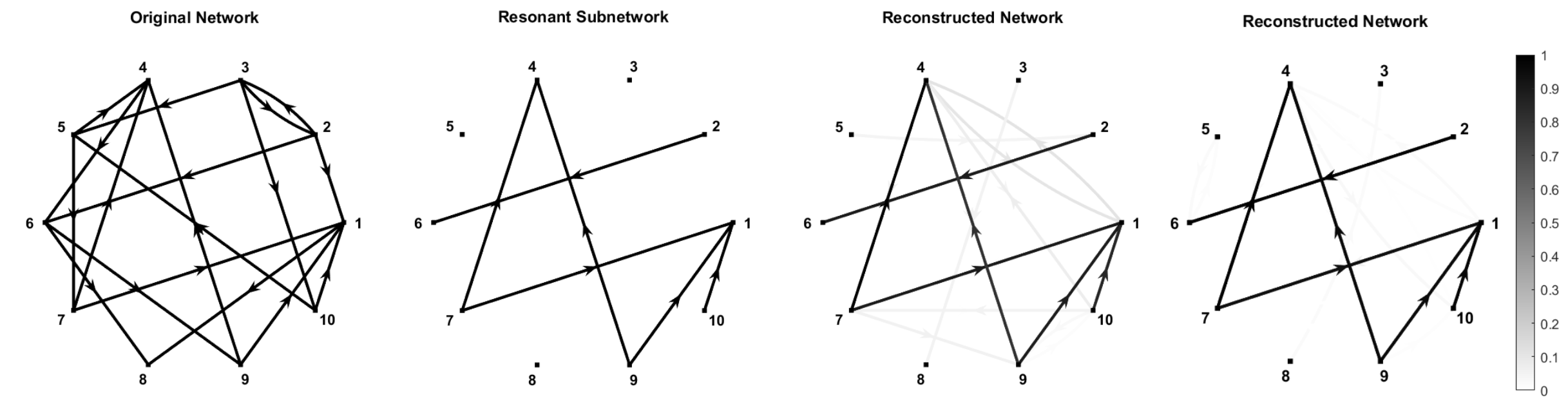
Refer to caption
Figure 5: Reconstruction of a Kuramoto network from numerical time series data. From left to right: original network that generated the time series; resonant subnetwork; reconstruction of the resonant subnetwork for ε=125\varepsilon=\frac{1}{25} from M=25M=25 observations; reconstruction of the resonant subnetwork for ε=1100\varepsilon=\frac{1}{100} from M=100M=100 observations.

An explicit error bound

For equations (56) we now derive an explicit theoretical bound on the reconstruction errors |a^i​j−ai​j||\hat{a}_{ij}-a_{ij}|. Recall that Theorem 5.1 gives a bound on the errors ‖A^j−Aj(1)‖∞\|\hat{A}_{j}-A_{j}^{(1)}\|_{\infty} in the reconstructed complex Fourier coefficients. These in turn lead to error bounds for the estimated a^i,j\hat{a}_{i,j}, because

|a^i​j−ai​j|=|A^j,ei−ej−A^j,ej−ei−Aj,ei−ej(1)+Aj,ej−ei(1)|\displaystyle|\hat{a}_{ij}-a_{ij}|=|\hat{A}_{j,e_{i}-e_{j}}-\hat{A}_{j,e_{j}-e_{i}}-A^{(1)}_{j,e_{i}-e_{j}}+A^{(1)}_{j,e_{j}-e_{i}}|
≤|A^j,ei−ej−Aj,ei−ej(1)|+|A^j,ej−ei−Aj,ej−ei(1)|\displaystyle\leq|\hat{A}_{j,e_{i}-e_{j}}-A^{(1)}_{j,e_{i}-e_{j}}|+|\hat{A}_{j,e_{j}-e_{i}}-A^{(1)}_{j,e_{j}-e_{i}}|
≤2​‖A^j−Aj(1)‖∞≤2​ℭj​‖Θ+‖∞​ε,\displaystyle\leq 2\|\hat{A}_{j}-A_{j}^{(1)}\|_{\infty}\leq 2\mathfrak{C}_{j}\|\Theta^{+}\|_{\infty}\sqrt{\varepsilon}\,,

where the final inequality follows from part 3 of Theorem 5.1. The following proposition provides an explicit upper bound for the constant ℭj\mathfrak{C}_{j}. For simplicity, we assume that the pure (non-detuned) frequencies satisfy

ωi≠ωj⟹|ωi−ωj|≥1.\omega_{i}\neq\omega_{j}\implies|\omega_{i}-\omega_{j}|\geq 1\,. (65)
Proposition 6.1.

Consider the classical Kuramoto system (56). Denote by dj:=∑i=1nai​jd_{j}:=\sum_{i=1}^{n}a_{ij} the in-degree of cell jj, and by dmax:=maxj⁡djd_{\rm max}:=\max_{j}d_{j} the maximal in-degree. Then the constant ℭj\mathfrak{C}_{j} in Theorem 5.1 is bounded by

ℭj≤ℭjmax:=12​dj​(dmax+4+2​L+Ω)+2​L.\mathfrak{C}_{j}\leq\mathfrak{C}_{j}^{\rm max}:=\frac{1}{2}d_{j}(d_{\rm max}+4+2L+\Omega)+2L\,. (66)
Proof.

Recall that the constant ℭj\mathfrak{C}_{j} appearing in Theorem 5.1 is given by ℭj=Aj+B~j+Cj+D~j\mathfrak{C}_{j}=A_{j}+\widetilde{B}_{j}+C_{j}+\widetilde{D}_{j} – see (50). So it suffices to recall the definitions of these constants, and to compute them for the example of the Kuramoto equations (56). To do this, note that (56) is of the form (16) with Rj(2)=0R_{j}^{(2)}=0, so that Rj(1):=Fj(1)+ε​Rj(2)=Fj(1)R_{j}^{(1)}:=F_{j}^{(1)}+\varepsilon R_{j}^{(2)}=F_{j}^{(1)}. This implies that Bj=0B_{j}=0, see (26). It is also clear from (56) that ‖Rj(1)‖0=‖Fj(1)‖0≤Ω+∑iai​j=Ω+dj\|R_{j}^{(1)}\|_{0}=\|F_{j}^{(1)}\|_{0}\leq\Omega+\sum_{i}a_{ij}=\Omega+d_{j}, and that ‖∂iFj(1)‖0=ai​j\|\partial_{i}F_{j}^{(1)}\|_{0}=a_{ij} for i≠ji\neq j. It thus follows from (24) that

Aj≤12​∑iai​j​(Ω+∑kak​i)≤12​dj​(Ω+dmax),A_{j}\leq\frac{1}{2}\sum_{i}a_{ij}(\Omega+\sum_{k}a_{ki})\leq\frac{1}{2}d_{j}(\Omega+d_{\rm max}),

and from (46) that

B~j≤∑iai​j​L=dj​L.\widetilde{B}_{j}\leq\sum_{i}a_{ij}L=d_{j}L\,.

Next, we split Fj(1)=Fj𝒦+Fjℛ+Fj𝒩F_{j}^{(1)}=F_{j}^{\mathcal{K}}+F_{j}^{\mathcal{R}}+F_{j}^{\mathcal{N}} in its library-part, its remaining resonant part, and its nonresonant part. Because the library 𝒦\mathcal{K} was chosen to contain all resonant terms in Fj(1)F^{(1)}_{j}, we have that Fjℛ=0F_{j}^{\mathcal{R}}=0, and thus that Cj=0C_{j}=0, see (34). Furthermore,

Fj𝒩​(ϕ)=∑ωi≠ωjai​j​sin⁡(ϕi−ϕj)=∑⟨k,ω⟩≠0Aj,k(1)​ei​⟨k,ϕ⟩.F_{j}^{\mathcal{N}}(\phi)=\sum_{\omega_{i}\neq\omega_{j}}a_{ij}\sin(\phi_{i}-\phi_{j})=\sum_{\langle k,\omega\rangle\neq 0}A_{j,k}^{(1)}e^{i\langle k,\phi\rangle}\,.

Using (65), it follows that

∑⟨k,ω⟩≠0|Aj,k(1)⟨k,ω⟩|≤∑⟨k,ω⟩≠0|Aj,k(1)|=∑ωi≠ωjai​j≤dj,\sum_{\langle k,\omega\rangle\neq 0}\left|\frac{A_{j,k}^{(1)}}{\langle k,\omega\rangle}\right|\leq\sum_{\langle k,\omega\rangle\neq 0}\left|A_{j,k}^{(1)}\right|=\sum_{\omega_{i}\neq\omega_{j}}a_{ij}\leq d_{j}\,,

so we may choose

Dj=2​dj,D_{j}=2d_{j}\,,

see (36), and D~j=Dj+2​L\widetilde{D}_{j}=D_{j}+2L, see (49). Together, our estimates for Aj,B~j,CjA_{j},\widetilde{B}_{j},C_{j} and D~j\widetilde{D}_{j} yield formula (66). ∎

7 Second order resonant reconstruction

The first order reconstruction method that we presented in the first part of this paper allows us to detect first order (in ε\varepsilon) resonant coupling terms in phase oscillator systems of the form (1). For instance, when ωi−ωj∼ε\omega_{i}-\omega_{j}\sim\varepsilon, the method can identify terms in the differential equations of the form ε​ai​j​sin⁡(ϕi−ϕj)\varepsilon a_{ij}\sin(\phi_{i}-\phi_{j}). By design, the method cannot detect nonresonant interactions. However, the interplay between nonresonant interactions at order ∼ε\sim\varepsilon can lead to dynamical behavior equivalent to that of a resonant interaction at order ∼ε2\sim\varepsilon^{2}. In the absence of resonant first order interactions, our second order resonant reconstruction method can detect such “emergent” second order interactions. In Appendix D, we explore how these emergent interactions are shaped by nonresonant first order interactions. For instance, we show how nonresonant dyadic interactions at order ∼ε\sim\varepsilon combine to form resonant triplet interactions at order ∼ε2\sim\varepsilon^{2}.

The key technical result underlying our second order resonant reconstruction method is the second order resonant normal form theorem. This theorem states that for any coupled oscillator system of the form (1) there exists a change of variables (diffeomorphism)

ΓH(1)ε:ϕ↦ψ:=ϕ+ε​H(1)​(ϕ)+𝒪​(ε2),\Gamma^{\varepsilon}_{H^{(1)}}:\phi\mapsto\psi:=\phi+\varepsilon H^{(1)}(\phi)+\mathcal{O}(\varepsilon^{2})\,,

defined for all ϕ∈𝕋n\phi\in\mathbb{T}^{n} and for small enough values of ε\varepsilon, with the property that ϕ​(t)\phi(t) satisfies (1) if and only if ψ​(t):=ΓH(1)ε​(ϕ​(t))\psi(t):=\Gamma^{\varepsilon}_{H^{(1)}}(\phi(t)) satisfies an ODE

ψ˙j=ωj+ε​F¯j(1)​(ψ)+ε2​F¯j(2)​(ψ)+ε3​R¯j(3)​(ϕ,ε),\dot{\psi}_{j}=\omega_{j}+\varepsilon\overline{F}_{j}^{(1)}(\psi)+\varepsilon^{2}\overline{F}_{j}^{(2)}(\psi)+\varepsilon^{3}\overline{R}_{j}^{(3)}(\phi,\varepsilon)\,, (67)

such that F¯(1)\overline{F}^{(1)} and F¯(2)\overline{F}^{(2)} are sums of resonant Fourier terms only, i.e.,

F¯j(1)​(ϕ)=∑⟨k,ω⟩=0Cj,k(1)​ei​⟨k,ϕ⟩​and​F¯j(2)​(ϕ)=∑⟨k,ω⟩=0Cj,k(2)​ei​⟨k,ϕ⟩,\overline{F}_{j}^{(1)}(\phi)=\sum_{\langle k,\omega\rangle=0}C_{j,k}^{(1)}e^{i\langle k,\phi\rangle}\ \mbox{and}\ \overline{F}_{j}^{(2)}(\phi)=\sum_{\langle k,\omega\rangle=0}C_{j,k}^{(2)}e^{i\langle k,\phi\rangle}\,,

for certain Fourier coefficients Cj,k(1),Cj,k(2)C_{j,k}^{(1)},C_{j,k}^{(2)}. We prove this fact in Appendices B, C and D. In particular, the solutions of (1) and (67) differ only by an amount of the order ∼ε\sim\varepsilon. The Fourier coefficients of F¯(1)\overline{F}^{(1)} and F¯(2)\overline{F}^{(2)} can be expressed in terms of the Fourier coefficients of the original vector field F(1)F^{(1)} and F(2)F^{(2)}. More precisely, we show in Theorem C.2 that

Cj,k(1)=Aj,k(1)​for all​k∈ℤn​with​⟨k,ω⟩=0,C_{j,k}^{(1)}=A_{j,k}^{(1)}\ \mbox{for all}\ k\in\mathbb{Z}^{n}\ \mbox{with}\ \langle k,\omega\rangle=0\,,

see also (116), while the formula for the Cj,k(2)C_{j,k}^{(2)} is more involved. If it so happens that F¯(1)=0\overline{F}^{(1)}=0, that is, if F(1)F^{(1)} does not contain any resonant terms, then (67) reduces to

ψ˙j=ωj+ε2​F¯j(2)​(ψ)+ε3​R¯j(3)​(ϕ,ε).\dot{\psi}_{j}=\omega_{j}+\varepsilon^{2}\overline{F}_{j}^{(2)}(\psi)+\varepsilon^{3}\overline{R}_{j}^{(3)}(\phi,\varepsilon)\,.

For this specific case, we provide a formula for the Cj,k(2)C_{j,k}^{(2)} in Theorem D.1. As was the case for the first-order method, our second-order resonant reconstruction method exploits the approximate linear relation between observed phase drifts and Fourier coefficients of the normal form. Let us again assume that we are given reasonable estimates of the coupling strength ε\varepsilon and the oscillator frequencies ω1,…​ωn\omega_{1},\ldots\omega_{n}, and that we have access to noisy phase signals

Φ(m)​(t)∈ℝn​with​ 1≤m≤M,\Phi^{(m)}(t)\in\mathbb{R}^{n}\ \mbox{with}\ 1\leq m\leq M\,,

this time at times

t=0​and​t=T:=1ε​ε.t=0\ \mbox{and}\ t=T:=\frac{1}{\varepsilon\sqrt{\varepsilon}}\,.

As before, the noise in these signals is assumed small and bounded, that is, there are constants Lj>0L_{j}>0 such that for every 1≤m≤M1\leq m\leq M, there is a (lift of an) exact solution ϕ(m)​(t)∈ℝn\phi^{(m)}(t)\in\mathbb{R}^{n} to (1) with

|ϕj(m)​(0)−Φj(m)​(0)|≤Lj​ε​and​|ϕj(m)​(T)−Φj(m)​(T)|≤Lj​ε.|\phi^{(m)}_{j}(0)-\Phi^{(m)}_{j}(0)|\leq L_{j}\varepsilon\ \mbox{and}\ |\phi^{(m)}_{j}(T)-\Phi^{(m)}_{j}(T)|\leq L_{j}\varepsilon\,. (68)

Our second order reconstruction method can then be summarized as follows:

  1. 1)

    Fix an oscillator 1≤j≤n1\leq j\leq n and calculate the rescaled observed drifts

    Δ(m):=Φj(m)​(T)−Φj(m)​(0)−ωj​Tε2​T∈ℝfor​ 1≤m≤M.{\Delta}^{(m)}:=\frac{\Phi^{(m)}_{j}(T)-\Phi^{(m)}_{j}(0)-\omega_{j}T}{\varepsilon^{2}T}\in\mathbb{R}\ \ \mbox{for}\ 1\leq m\leq M\,.

    These drifts together form a (column) vector Δ∈ℝM\Delta\in\mathbb{R}^{M}.

  2. 2)

    Select a finite library of resonant Fourier labels

    𝒦={k1,…,kK}⊂{k∈ℤn|⟨k,ω⟩=0},\mathcal{K}=\{k_{1},\ldots,k_{K}\}\subset\{k\in\mathbb{Z}^{n}\,|\,\langle k,\omega\rangle=0\}\,,

    where K:=|𝒦|K:=|\mathcal{K}|, and create the library matrix

    Θ:=(ei​⟨k1,Φ(1)​(0)⟩…ei​⟨kK,Φ(1)​(0)⟩⋮⋱⋮ei​⟨k1,Φ(M)​(0)⟩…ei​⟨kK,Φ(M)​(0)⟩):ℂK→ℂM.\Theta:=\left(\begin{array}[]{ccc}e^{i\langle k_{1},\Phi^{(1)}(0)\rangle}&\ldots&e^{i\langle k_{K},\Phi^{(1)}(0)\rangle}\\ \vdots&\ddots&\vdots\\ e^{i\langle k_{1},\Phi^{(M)}(0)\rangle}&\ldots&e^{i\langle k_{K},\Phi^{(M)}(0)\rangle}\end{array}\right):\mathbb{C}^{K}\to\mathbb{C}^{M}\,.

    We assume that Θ\Theta is injective.

  3. 3)

    List the resonant Fourier coefficients Cj,k(2)C_{j,k}^{(2)} (with k∈𝒦k\in\mathcal{K}) in the vector

    Cj(2):=(Cj,k1(2),…,Cj,kK(2))T∈ℂK.C_{j}^{(2)}:=(C^{(2)}_{j,k_{1}},\ldots,C^{(2)}_{j,k_{K}})^{T}\in\mathbb{C}^{K}\,.

    We estimate this vector by the vector

    C^j=(C^j,k1,…,C^j,kK)T∈ℂK\hat{C}_{j}=(\hat{C}_{j,k_{1}},\ldots,\hat{C}_{j,k_{K}})^{T}\in\mathbb{C}^{K}

    defined by

    C^j=arg⁡minB∈ℂK​∑m=1M|Δ(m)−∑i=1KBki​ei​⟨ki,Φ(m)​(0)⟩|2∈ℂK.\hat{C}_{j}={\arg\min}_{B\in\mathbb{C}^{K}}\sum_{m=1}^{M}\left|\Delta^{(m)}-\sum_{i=1}^{K}B_{k_{i}}e^{i\langle k_{i},\Phi^{(m)}(0)\rangle}\right|^{2}\in\mathbb{C}^{K}\,.

    This minimizer is given by

    C^j=Θ+​(Δ)∈ℂK.\hat{C}_{j}=\Theta^{+}(\Delta)\in\mathbb{C}^{K}\,. (69)

In the next section, we prove that the estimators C^j,k\hat{C}_{j,k} are good approximations of the true normal form coefficients Cj,k(2)C_{j,k}^{(2)} under some natural conditions. This proof is highly similar to the corresponding proof for the first order reconstruction method.

8 Validity of second order reconstruction

The main result of this section is Theorem 8.1, which is the analogue of Theorem 5.1 for the second order resonant reconstruction method. The statement in Theorem 8.1 may appear complicated, but its proof is highly similar to that of Lemmas 4.1 and 4.2 and Theorem 5.1.

Note that it is not assumed in Theorem 8.1 that equations (1) can be brought into normal form exactly (in which case F¯(1)=F¯𝒩=0\overline{F}^{(1)}=\overline{F}^{\mathcal{N}}=0). Instead, it suffices that the equations can be transformed into normal form approximately.

Theorem 8.1.

For |ε|≤ε0|\varepsilon|\leq\varepsilon_{0} consider the phase equations

ϕ˙j=ωj+ε​Fj(1)​(ϕ)+ε2​Fj(2)​(ϕ)+ε3​Rj(3)​(ϕ,ε)​for all​ 1≤j≤n.\dot{\phi}_{j}=\omega_{j}+\varepsilon F_{j}^{(1)}(\phi)+\varepsilon^{2}F_{j}^{(2)}(\phi)+\varepsilon^{3}R_{j}^{(3)}(\phi,\varepsilon)\ \mbox{for all}\ 1\leq j\leq n\,. (70)

We assume that there exists a family of continuously differentiable “approximate normal form transformations” Γε:𝕋n→𝕋n\Gamma^{\varepsilon}:\mathbb{T}^{n}\to\mathbb{T}^{n} with the property that ϕ​(t)\phi(t) is a solution to (70) if and only if ψ​(t)=Γε​(ϕ​(t))\psi(t)=\Gamma^{\varepsilon}(\phi(t)) satisfies

ψ˙j=ωj+ε​F¯j(1)​(ϕ)+ε2​F¯j(2)​(ϕ)+ε3​R¯(3)​(ϕ,ε),\dot{\psi}_{j}=\omega_{j}+\varepsilon\overline{F}_{j}^{(1)}(\phi)+\varepsilon^{2}\overline{F}_{j}^{(2)}(\phi)+\varepsilon^{3}\overline{R}^{(3)}(\phi,\varepsilon)\,, (71)

where F¯j(1)∈C2​(𝕋n)\overline{F}^{(1)}_{j}\in C^{2}(\mathbb{T}^{n}), F¯j(2)∈C1​(𝕋n)\overline{F}^{(2)}_{j}\in C^{1}(\mathbb{T}^{n}) and R¯j(3)∈C0​(𝕋n×[−ε0,ε0])\overline{R}^{(3)}_{j}\in C^{0}(\mathbb{T}^{n}\times[-\varepsilon_{0},\varepsilon_{0}]).

Let 𝒦={k1,…,kK}⊂{k∈ℤn|⟨k,ω⟩=0}\mathcal{K}=\{k_{1},\ldots,k_{K}\}\subset\{k\in\mathbb{Z}^{n}\,|\,\langle k,\omega\rangle=0\} be a library of resonant Fourier labels, and decompose the second order normal form term as

F¯j(2)=F¯j𝒦+F¯jℛ+F¯j𝒩,\overline{F}_{j}^{(2)}=\overline{F}_{j}^{\mathcal{K}}+\overline{F}_{j}^{\mathcal{R}}+\overline{F}_{j}^{\mathcal{N}}\ ,

in which

F¯j𝒦​(ϕ)\displaystyle\overline{F}_{j}^{\mathcal{K}}(\phi) :=∑k∈𝒦Cj,k(2)​ei​⟨k,ϕ⟩,\displaystyle:=\sum_{k\in\mathcal{K}}C_{j,k}^{(2)}e^{i\langle k,\phi\rangle}\,, (72)
F¯jℛ​(ϕ)\displaystyle\overline{F}_{j}^{\mathcal{R}}(\phi) :=∑⟨k,ω⟩=0,k∉𝒦Cj,k(2)​ei​⟨k,ϕ⟩,\displaystyle:=\sum_{\langle k,\omega\rangle=0,\,k\notin\mathcal{K}}C_{j,k}^{(2)}e^{i\langle k,\phi\rangle}\,, (73)
F¯j𝒩​(ϕ)\displaystyle\overline{F}_{j}^{\mathcal{N}}(\phi) :=∑⟨k,ω⟩≠0Cj,k(2)​ei​⟨k,ϕ⟩.\displaystyle:=\sum_{\langle k,\omega\rangle\neq 0}C_{j,k}^{(2)}e^{i\langle k,\phi\rangle}\,. (74)

Assume the following on the transformation and approximate normal form:

  • i)

    The transformations Γε\Gamma^{\varepsilon} are close to the identity: there are constants H1,…,Hn>0H_{1},\ldots,H_{n}>0 such that

    |Γε​(ϕ)j−ϕj|≤Hj​ε,|\Gamma^{\varepsilon}(\phi)_{j}-\phi_{j}|\leq H_{j}\varepsilon\,, (75)

    for all |ε|≤ε0|\varepsilon|\leq\varepsilon_{0}, all ϕ∈𝕋n\phi\in\mathbb{T}^{n}, and all 1≤j≤n.1\leq j\leq n.

  • ii)

    The first order normal form nearly vanishes: there are constants G1,…,Gn>0G_{1},\ldots,G_{n}>0 such that

    |F¯j(1)​(ϕ)|≤ε2​Gj,|\overline{F}_{j}^{(1)}(\phi)|\leq\varepsilon^{2}G_{j}\,, (76)

    for all |ε|≤ε0|\varepsilon|\leq\varepsilon_{0}, all ϕ∈𝕋n\phi\in\mathbb{T}^{n}, and all 1≤j≤n.1\leq j\leq n.

  • iii)

    The library 𝒦\mathcal{K} captures the most prominent resonant terms in F¯(2)\overline{F}^{(2)}: there are constants C1,…,Cn>0C_{1},\ldots,C_{n}>0 such that

    |∫0TF¯jℛ​(ϕ+ω​t)​𝑑t|≤Cj​ε​T,\left|\int_{0}^{T}\overline{F}_{j}^{\mathcal{R}}(\phi+\omega t)\,dt\right|\leq C_{j}\sqrt{\varepsilon}T\,, (77)

    for all |ε|≤ε0|\varepsilon|\leq\varepsilon_{0}, all ϕ∈𝕋n\phi\in\mathbb{T}^{n}, and all 1≤j≤n.1\leq j\leq n.

  • iv)

    The nonresonant terms in F¯(2)\overline{F}^{(2)} have a bounded dynamical effect: there are constants D1,…,Dn>0D_{1},\ldots,D_{n}>0 such that

    |∫0TF¯j𝒩​(ϕ+ω​t)​𝑑t|≤Dj,\left|\int_{0}^{T}\overline{F}_{j}^{\mathcal{N}}(\phi+\omega t)\,dt\right|\leq D_{j}\,, (78)

    for all |ε|≤ε0|\varepsilon|\leq\varepsilon_{0}, all ϕ∈𝕋n\phi\in\mathbb{T}^{n}, and all 1≤j≤n.1\leq j\leq n.

Denote by

Cj(2)=(Cj,k1(2),…,Cj,kK(2))T∈ℂK​and​C^j=(C^j,k1,…,C^j,kK)T∈ℂKC_{j}^{(2)}=(C_{j,k_{1}}^{(2)},\ldots,C_{j,k_{K}}^{(2)})^{T}\in\mathbb{C}^{K}\ \mbox{and}\ \hat{C}_{j}=(\hat{C}_{j,k_{1}},\ldots,\hat{C}_{j,k_{K}})^{T}\in\mathbb{C}^{K}

respectively the vector of true resonant Fourier coefficients Cj,k(2)C_{j,k}^{(2)} in F¯j(2)\overline{F}_{j}^{(2)}, and the vector of their estimates C^j,k\hat{C}_{j,k} provided by our second order resonant reconstruction method. Let ℭj\mathfrak{C}_{j} be the constant given in (92) below, which is independent of ε,K\varepsilon,K and MM. Then

  1. 1.

    The l1l_{1}-distance between C^j\hat{C}_{j} and Cj(2)C_{j}^{(2)} satisfies

    ‖C^j−Cj(2)‖1≤M​ℭj​‖Θ+‖1​ε;\|\hat{C}_{j}-C_{j}^{(2)}\|_{1}\leq M\mathfrak{C}_{j}\|\Theta^{+}\|_{1}\sqrt{\varepsilon}\,;
  2. 2.

    The l2l_{2}-distance between C^j\hat{C}_{j} and Cj(2)C_{j}^{(2)} satisfies

    ‖C^j−Cj(2)‖2≤M​ℭj​‖Θ+‖2​ε;\|\hat{C}_{j}-C_{j}^{(2)}\|_{2}\leq\sqrt{M}\mathfrak{C}_{j}\|\Theta^{+}\|_{2}\sqrt{\varepsilon}\,;
  3. 3.

    The l∞l_{\infty}-distance between C^j\hat{C}_{j} and Cj(2)C_{j}^{(2)} satisfies

    ‖C^j−Cj(2)‖∞≤ℭj​‖Θ+‖∞​ε.\|\hat{C}_{j}-C_{j}^{(2)}\|_{\infty}\leq\mathfrak{C}_{j}\|\Theta^{+}\|_{\infty}\sqrt{\varepsilon}\,.
Proof.

Recall the assumption in (68) that Φ(m)​(0)\Phi^{(m)}(0) and Φ(m)​(T)\Phi^{(m)}(T) are observations of true solutions t↦ϕ(m)​(t)t\mapsto\phi^{(m)}(t) to (70) that satisfy

|ϕj(m)​(0)−Φj(m)​(0)|≤Lj​ε​and​|ϕj(m)​(T)−Φj(m)​(T)|≤Lj​ε.|\phi^{(m)}_{j}(0)-\Phi^{(m)}_{j}(0)|\leq L_{j}\varepsilon\ \mbox{and}\ |\phi^{(m)}_{j}(T)-\Phi^{(m)}_{j}(T)|\leq L_{j}\varepsilon\,.

For each such true solution ϕ​(t)\phi(t), let us define ψ​(t):=Γε​(ϕ​(t))\psi(t):=\Gamma^{\varepsilon}(\phi(t)). Then it follows from (75) that

|ψj(m)​(t)−ϕj(m)​(t)|≤Hj​ε​for all​t,|\psi_{j}^{(m)}(t)-\phi^{(m)}_{j}(t)|\leq H_{j}\varepsilon\ \mbox{for all}\ t\,, (79)

and hence also that

|ψj(m)​(t)−Φj(m)​(t)|≤(Lj+Hj)​εfor​t∈{0,T}.|\psi_{j}^{(m)}(t)-\Phi^{(m)}_{j}(t)|\leq(L_{j}+H_{j})\varepsilon\ \ \mbox{for}\ t\in\{0,T\}\,. (80)

We can now define the true rescaled normal form drifts

δ(m):=ψj(m)​(T)−ψj(m)​(0)−ωj​Tε2​T.\delta^{(m)}:=\frac{\psi_{j}^{(m)}(T)-\psi_{j}^{(m)}(0)-\omega_{j}T}{\varepsilon^{2}T}\,. (81)

The observed rescaled drifts are good approximations of these true rescaled drifts, as it follows immediately from (80) that

|Δ(m)−δ(m)|≤2​(Lj+Hj)ε​T.|\Delta^{(m)}-\delta^{(m)}|\leq\frac{2(L_{j}+H_{j})}{\varepsilon T}\,. (82)

Note that this expression is of the order ∼ε\sim\sqrt{\varepsilon} for T∼1ε​εT\sim\frac{1}{\varepsilon\sqrt{\varepsilon}}.

We now proceed to express δ(m)\delta^{(m)} in terms of the Fourier coefficients Cj,k(2)C_{j,k}^{(2)} of the second order normal form, just like we did for the first order reconstruction method in Sections 4 and 5. In order to do this, note that integration of (71) from t=0t=0 to t=Tt=T yields that

ψj(m)​(T)−\displaystyle\psi_{j}^{(m)}(T)\,-\, ψj(m)​(0)−ωj​T=ε​∫0TF¯j(1)​(ψ(m)​(t))​𝑑t\displaystyle\psi_{j}^{(m)}(0)-\omega_{j}T=\ \varepsilon\int_{0}^{T}\overline{F}_{j}^{(1)}(\psi^{(m)}(t))dt\
+ε2​∫0TF¯j(2)​(ψ(m)​(t))​𝑑t+ε3​∫0TR¯j(3)​(ψ(m)​(t),ε)​𝑑t.\displaystyle+\varepsilon^{2}\int_{0}^{T}\overline{F}_{j}^{(2)}(\psi^{(m)}(t))dt+\varepsilon^{3}\int_{0}^{T}\overline{R}_{j}^{(3)}(\psi^{(m)}(t),\varepsilon)dt\,. (83)

We rewrite and estimate the three integral terms on the right hand side of (83). The first and third integral terms in (83) are easy to bound:

|ε​∫0TF¯j(1)​(ψ(m)​(t))​𝑑t|≤ε3​T​Gj,\displaystyle\left|\varepsilon\int_{0}^{T}\overline{F}_{j}^{(1)}(\psi^{(m)}(t))dt\right|\leq\varepsilon^{3}TG_{j}\,, (84)
|ε3​∫0TR¯j(3)​(ψ(m)​(t),ε)​𝑑t|≤ε3​T​‖R¯j(3)‖0,\displaystyle\left|\varepsilon^{3}\int_{0}^{T}\overline{R}_{j}^{(3)}(\psi^{(m)}(t),\varepsilon)dt\right|\leq\varepsilon^{3}T\|\overline{R}^{(3)}_{j}\|_{0}\,, (85)

where (84) clearly follows from (76). We investigate the second integral term in (83) by mimicking the proof of Lemmas 4.1 and 4.2. The first step is to note that integration of (71) from s=0s=0 to s=ts=t gives

ψi(m)​(t)=ψi(m)​(0)+ωi​t+ri​(t,ε),\psi_{i}^{(m)}(t)=\psi_{i}^{(m)}(0)+\omega_{i}t+r_{i}(t,\varepsilon)\ ,

for certain functions ri​(t,ε)r_{i}(t,\varepsilon) satisfying

|ri​(t,ε)|\displaystyle|r_{i}(t,\varepsilon)| ≤ε2​t​(ε−1​‖F¯i(1)‖0+‖F¯i(2)‖0+ε​‖R¯i(3)‖0)\displaystyle\leq\varepsilon^{2}t\left(\varepsilon^{-1}\|\overline{F}_{i}^{(1)}\|_{0}+\|\overline{F}_{i}^{(2)}\|_{0}+\varepsilon\|\overline{R}_{i}^{(3)}\|_{0}\right)
≤ε2​t​(ε​Gi+‖F¯i(2)‖0+ε​‖R¯i(3)‖0).\displaystyle\leq\varepsilon^{2}t\left(\varepsilon G_{i}+\|\overline{F}_{i}^{(2)}\|_{0}+\varepsilon\|\overline{R}_{i}^{(3)}\|_{0}\right)\,. (86)

As in the proof of Lemma 4.1, we can therefore estimate

|ε2​∫0TF¯j(2)​(ψ(m)​(t))​𝑑t−ε2​∫0TF¯j(2)​(ψ(m)​(0)+ω​t)​𝑑t|\displaystyle\left|\varepsilon^{2}\int_{0}^{T}\overline{F}_{j}^{(2)}(\psi^{(m)}(t))dt-\varepsilon^{2}\int_{0}^{T}\overline{F}_{j}^{(2)}(\psi^{(m)}(0)+\omega t)dt\right|
≤ε2​∫0T∑i=1n‖∂iF¯j(2)‖0​|ri​(t,ε)|​d​t≤Aj​ε4​T2.\displaystyle\leq\varepsilon^{2}\int_{0}^{T}\sum_{i=1}^{n}\|\partial_{i}\overline{F}_{j}^{(2)}\|_{0}|r_{i}(t,\varepsilon)|dt\leq A_{j}\varepsilon^{4}T^{2}\,. (87)

in which

Aj=12​∑i=1n‖∂iF¯j(2)‖0​(ε0​Gi+‖F¯i(2)‖0+ε0​‖R¯i(3)‖0).A_{j}=\frac{1}{2}\sum_{i=1}^{n}\|\partial_{i}\overline{F}_{j}^{(2)}\|_{0}\left(\varepsilon_{0}G_{i}+\|\overline{F}_{i}^{(2)}\|_{0}+\varepsilon_{0}\|\overline{R}_{i}^{(3)}\|_{0}\right)\,.

Next, in view of (80),

|ε2​∫0TF¯j(2)​(ψ(m)​(0)+ω​t)​𝑑t−ε2​∫0TF¯j(2)​(Φ(m)​(0)+ω​t)​𝑑t|\displaystyle\left|\varepsilon^{2}\int_{0}^{T}\overline{F}_{j}^{(2)}(\psi^{(m)}(0)+\omega t)dt-\varepsilon^{2}\int_{0}^{T}\overline{F}_{j}^{(2)}(\Phi^{(m)}(0)+\omega t)dt\right|
≤Bj​ε3​Tin which​Bj:=∑i=1n‖∂iF¯j(2)‖0​(Li+Hi).\displaystyle\leq B_{j}\varepsilon^{3}T\ \ \mbox{in which}\ B_{j}:=\sum_{i=1}^{n}\|\partial_{i}\overline{F}_{j}^{(2)}\|_{0}(L_{i}+H_{i})\,. (88)

We continue by mimicking the proof of Lemma 4.2. Recalling that F¯j(2)=F¯j𝒦+F¯jℛ+F¯j𝒩\overline{F}_{j}^{(2)}=\overline{F}_{j}^{\mathcal{K}}+\overline{F}_{j}^{\mathcal{R}}+\overline{F}_{j}^{\mathcal{N}}, we estimate

|ε2​∫0TF¯j(2)​(Φ(m)​(0)+ω​t)​𝑑t−ε2​T​∑k∈𝒦Cj,k(2)​ei​⟨k,Φ(m)​(0)⟩|\displaystyle\left|\varepsilon^{2}\int_{0}^{T}\overline{F}_{j}^{(2)}(\Phi^{(m)}(0)+\omega t)dt-\varepsilon^{2}T\sum_{k\in\mathcal{K}}C^{(2)}_{j,k}e^{i\langle k,\Phi^{(m)}(0)\rangle}\right|
≤ε2​|∫0TF¯jℛ​(Φ(m)​(0)+ω​t)​𝑑t|+ε2​|∫0TF¯j𝒩​(Φ(m)​(0)+ω​t)​𝑑t|\displaystyle\leq\varepsilon^{2}\left|\int_{0}^{T}\overline{F}_{j}^{\mathcal{R}}(\Phi^{(m)}(0)+\omega t)dt\right|+\varepsilon^{2}\left|\int_{0}^{T}\overline{F}_{j}^{\mathcal{N}}(\Phi^{(m)}(0)+\omega t)dt\right|
≤Cj​ε52​T+ε2​Dj,\displaystyle\leq C_{j}\varepsilon^{\frac{5}{2}}T+\varepsilon^{2}D_{j}\,, (89)

where the inequalities in the last line follow from assumptions (77) and (78). Combining (83) with (84), (85), (87), (88) and (89) yields

|ψj(m)​(T)−ψj(m)​(0)−ωj​T−ε2​T​∑k∈𝒦Cj,k(2)​ei​⟨k,Φ(m)​(0)⟩|\displaystyle\left|\psi^{(m)}_{j}(T)-\psi^{(m)}_{j}(0)-\omega_{j}T-\varepsilon^{2}T\sum_{k\in\mathcal{K}}C^{(2)}_{j,k}e^{i\langle k,\Phi^{(m)}(0)\rangle}\right|
≤Aj​ε4​T2+ε3​T​(Bj+Gj+‖R¯j(3)‖0)+Cj​ε52​T+ε2​Dj.\displaystyle\leq A_{j}\varepsilon^{4}T^{2}+\varepsilon^{3}T(B_{j}+G_{j}+\|\overline{R}_{j}^{(3)}\|_{0})+C_{j}\varepsilon^{\frac{5}{2}}T+\varepsilon^{2}D_{j}\,. (90)

Next, combining (90) with (81) and (82) we obtain

|Δ(m)−∑k∈𝒦Cj,k(2)​ei​⟨k,Φ(m)​(0)⟩|\displaystyle\left|\Delta^{(m)}-\sum_{k\in\mathcal{K}}C^{(2)}_{j,k}e^{i\langle k,\Phi^{(m)}(0)\rangle}\right|
≤|Δ(m)−δ(m)|+|δ(m)−∑k∈𝒦Cj,k(2)​ei​⟨k,Φ(m)​(0)⟩|\displaystyle\leq\left|\Delta^{(m)}-\delta^{(m)}\right|+\left|\delta^{(m)}-\sum_{k\in\mathcal{K}}C^{(2)}_{j,k}e^{i\langle k,\Phi^{(m)}(0)\rangle}\right|
≤2​(Lj+Hj)ε​T+Aj​ε2​T+ε​(Bj+Gj+‖R¯j(3)‖0)+Cj​ε+Dj/T.\displaystyle\leq\frac{2(L_{j}+H_{j})}{\varepsilon T}+A_{j}\varepsilon^{2}T+\varepsilon(B_{j}+G_{j}+\|\overline{R}_{j}^{(3)}\|_{0})+C_{j}\sqrt{\varepsilon}+D_{j}/T\,. (91)

For T=1ε​εT=\frac{1}{\varepsilon\sqrt{\varepsilon}}, the expression on the right hand side of (91) simplifies to

(2​(Lj+Hj)+Aj+Cj+ε​(Bj+Gj+‖R¯j(3)‖0)+ε​Dj)​ε≤ℭj​ε\left(2(L_{j}+H_{j})+A_{j}+C_{j}+\sqrt{\varepsilon}(B_{j}+G_{j}+\|\overline{R}_{j}^{(3)}\|_{0})+\varepsilon D_{j}\right)\sqrt{\varepsilon}\leq\mathfrak{C}_{j}\sqrt{\varepsilon}

in which

ℭj:=2​(Lj+Hj)+Aj+Cj+ε0​(Bj+Gj+‖R¯j(3)‖0)+ε0​Dj.\mathfrak{C}_{j}:=2(L_{j}+H_{j})+A_{j}+C_{j}+\sqrt{\varepsilon_{0}}(B_{j}+G_{j}+\|\overline{R}_{j}^{(3)}\|_{0})+\varepsilon_{0}D_{j}\,. (92)

To summarize, we proved that

Δ(m)=∑k∈𝒦Cj,k(2)​ei​⟨k,Φ(m)​(0)⟩+ρ(m),\Delta^{(m)}=\sum_{k\in\mathcal{K}}C^{(2)}_{j,k}e^{i\langle k,\Phi^{(m)}(0)\rangle}+\rho^{(m)}\,, (93)

where ρ(m)∈ℝ\rho^{(m)}\in\mathbb{R} satisfies the bound |ρ(m)|≤ℭj​ε|\rho^{(m)}|\leq\mathfrak{C}_{j}\sqrt{\varepsilon}. In particular, the vector ρ∈ℝM\rho\in\mathbb{R}^{M} satisfies equations (51), (52) and (53).

One can write equations (93) as an equality of MM-vectors

Δ=Θ​(Cj(2))+ρ.\Delta=\Theta(C_{j}^{(2)})+\rho\,.

Now we recall that our second order resonant reconstruction method chooses the estimated normal form coefficients to be C^j=Θ+​(Δ)\hat{C}_{j}=\Theta^{+}(\Delta), see (69). As a result,

C^j−Cj(2)=Θ+​(Δ)−Θ+​Θ​(Cj(2))=Θ+​(Δ)−Θ+​(Δ)+Θ+​(ρ)=Θ+​(ρ).\hat{C}_{j}-C_{j}^{(2)}=\Theta^{+}(\Delta)-\Theta^{+}\Theta(C_{j}^{(2)})=\Theta^{+}(\Delta)-\Theta^{+}(\Delta)+\Theta^{+}(\rho)=\Theta^{+}(\rho)\,.

The estimates on the norms ‖C^j−Cj(2)‖1,2,∞\|\hat{C}_{j}-C_{j}^{(2)}\|_{1,2,\infty} now follow from the argument that was already given in the proof of Theorem 5.1. ∎

9 A second order example

To illustrate the second order resonant reconstruction method introduced in Section 7, we consider the phase oscillator network

ϕ˙1\displaystyle\dot{\phi}_{1} =1+ε​sin⁡(ϕ5−ϕ1),\displaystyle=1+\varepsilon\,\sin(\phi_{5}-\phi_{1})\,, (94)
ϕ˙2\displaystyle\dot{\phi}_{2} =3+ε​(sin⁡(ϕ1−ϕ2)+sin⁡(ϕ3−ϕ2)),\displaystyle=3+\varepsilon\left(\sin(\phi_{1}-\phi_{2})+\sin(\phi_{3}-\phi_{2})\right)\,,
ϕ˙3\displaystyle\dot{\phi}_{3} =1+ε​sin⁡(ϕ4−ϕ3),\displaystyle=1+\varepsilon\,\sin(\phi_{4}-\phi_{3})\,,
ϕ˙4\displaystyle\dot{\phi}_{4} =5,\displaystyle=5\,,
ϕ˙5\displaystyle\dot{\phi}_{5} =3+ε​(sin⁡(ϕ3−ϕ5)+sin⁡(ϕ4−ϕ5)),\displaystyle=3+\varepsilon\left(\sin(\phi_{3}-\phi_{5})+\sin(\phi_{4}-\phi_{5})\right)\,,

of five weakly coupled phase oscillators with frequency vector

ω=(1,3,1,5,3).\omega=\left(1,3,1,5,3\right). (95)

We depict this network in Figure 6. Note that the first order normal form of equations (94) vanishes, as none of the interactions on the right hand side of (94) is resonant. We therefore do not attempt to reconstruct equations (94). Instead, we try to numerically approximate the second order resonant normal form of (94) from noisy observations of its solutions.
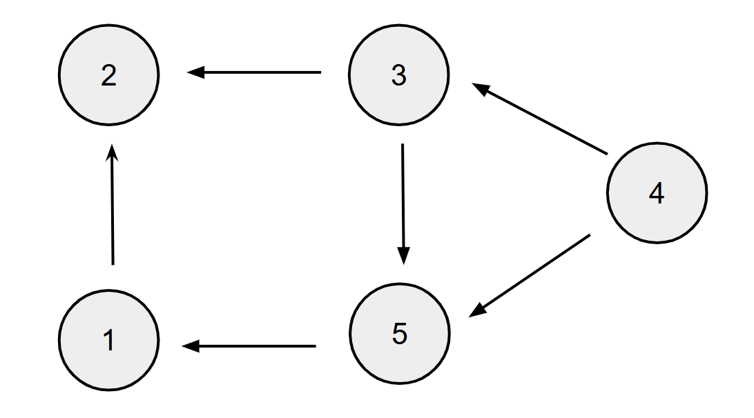
Refer to caption
Figure 6: Visualization of the network structure of equations (94).

In the selection of the reconstruction library for each oscillator, we anticipate that the second order part F¯j(2)\overline{F}_{j}^{(2)} of the normal form will be a linear combination of complex exponential functions (sines and cosines) that depend on resonant combination angles of the form

±(ϕj−ϕi)±(ϕi−ϕk)​for certain​ 1≤i,k≤n.\pm(\phi_{j}-\phi_{i})\pm(\phi_{i}-\phi_{k})\ \mbox{for certain}\ 1\leq i,k\leq n\,.

For example, for j=1j=1, the only such resonant combination angles are 0,±(ϕ1−ϕ3),±(2​ϕ1−2​ϕ3),±(ϕ2−ϕ5),±(ϕ1−2​ϕ2+ϕ4)0,\pm(\phi_{1}-\phi_{3}),\pm(2\phi_{1}-2\phi_{3}),\pm(\phi_{2}-\phi_{5}),\pm(\phi_{1}-2\phi_{2}+\phi_{4}), and ±(ϕ1+ϕ4−2​ϕ5)\pm(\phi_{1}+\phi_{4}-2\phi_{5}). Similarly, for j=2j=2, the only possibilities are 0,±(ϕ1−ϕ3)0,\pm(\phi_{1}-\phi_{3}), ±(ϕ2−ϕ5)\pm(\phi_{2}-\phi_{5}), ±(2​ϕ2−2​ϕ5)\pm(2\phi_{2}-2\phi_{5}), ±(ϕ1−2​ϕ2+ϕ4)\pm(\phi_{1}-2\phi_{2}+\phi_{4}), and ±(2​ϕ2−ϕ3−ϕ4)\pm(2\phi_{2}-\phi_{3}-\phi_{4}). Etc. Based on this principle, we choose the reconstruction libraries

𝒦1=\displaystyle\mathcal{K}_{1}= {α0,±α1,±α2,±α3,±α5,±α6},\displaystyle\{\alpha_{0},\pm\alpha_{1},\pm\alpha_{2},\pm\alpha_{3},\pm\alpha_{5},\pm\alpha_{6}\}\,,
𝒦2=\displaystyle\mathcal{K}_{2}= {α0,±α1,±α3,±α4,±α5,±α7},\displaystyle\{\alpha_{0},\pm\alpha_{1},\pm\alpha_{3},\pm\alpha_{4},\pm\alpha_{5},\pm\alpha_{7}\}\,,
𝒦3=\displaystyle\mathcal{K}_{3}= {α0,±α1,±α2,±α3,±α7,±α8},\displaystyle\{\alpha_{0},\pm\alpha_{1},\pm\alpha_{2},\pm\alpha_{3},\pm\alpha_{7},\pm\alpha_{8}\}\,,
𝒦4=\displaystyle\mathcal{K}_{4}= {α0,±α1,±α3,±α5,±α6,±α7,±α8},\displaystyle\{\alpha_{0},\pm\alpha_{1},\pm\alpha_{3},\pm\alpha_{5},\pm\alpha_{6},\pm\alpha_{7},\pm\alpha_{8}\}\,,
𝒦5=\displaystyle\mathcal{K}_{5}= {α0,±α1,±α3,±α4,±α6±α8},\displaystyle\{\alpha_{0},\pm\alpha_{1},\pm\alpha_{3},\pm\alpha_{4},\pm\alpha_{6}\pm\alpha_{8}\}\,,

in which

α0\displaystyle\alpha_{0} =0,\displaystyle=0\,,
α1\displaystyle\alpha_{1} =e1−e3,\displaystyle=e_{1}-e_{3}\,,
α2\displaystyle\alpha_{2} =2​e1−2​e3,\displaystyle=2e_{1}-2e_{3}\,,
α3\displaystyle\alpha_{3} =e2−e5,\displaystyle=e_{2}-e_{5}\,,
α4\displaystyle\alpha_{4} =2​e2−2​e5,\displaystyle=2e_{2}-2e_{5}\,,
α5\displaystyle\alpha_{5} =e1−2​e2+e4,\displaystyle=e_{1}-2e_{2}+e_{4}\,,
α6\displaystyle\alpha_{6} =e1+e4−2​e5,\displaystyle=e_{1}+e_{4}-2e_{5}\,,
α7\displaystyle\alpha_{7} =2​e2−e3−e4,\displaystyle=2e_{2}-e_{3}-e_{4}\,,
α8\displaystyle\alpha_{8} =e3+e4−2​e5.\displaystyle=e_{3}+e_{4}-2e_{5}\,.

The Fourier labels α1,…,α8\alpha_{1},\ldots,\alpha_{8} represent the possible dyadic and triadic interactions in the reconstructed second order normal form. A visualization of the interpretation of these interactions is given in Figure 7. We also note that the libraries together contain a total of 5757 elements. Our reconstruction method will thus determine 5757 different Fourier coefficients.

Refer to caption
Figure 7: Visualization of the second order resonant Fourier labels α1,…,α8\alpha_{1},\dots,\alpha_{8} used in the reconstruction libraries for equations (94).

We numerically reconstruct the second-order normal form of (94) by setting ε=1100\varepsilon=\frac{1}{100}, and choosing M=50M=50 initial phases ϕ(m)​(0)\phi^{(m)}(0) randomly from the uniform distribution on 𝕋5\mathbb{T}^{5}. Equations (94) are then integrated in MATLAB starting from these initial conditions, over a time-interval of the length T=1ε​ε=1000T=\frac{1}{\varepsilon\sqrt{\varepsilon}}=1000, to produce the final phases ϕ(m)​(T)\phi^{(m)}(T). A small uniformly random perturbation is also added to ϕ(m)​(0)\phi^{(m)}(0) and ϕ(m)​(T)\phi^{(m)}(T), producing the noisy phases Φ(m)​(0)\Phi^{(m)}(0) and Φ(m)​(T)\Phi^{(m)}(T). The maximal amplitude of this perturbation is chosen to be ε\varepsilon, that is, Lj=1L_{j}=1 for all 1≤j≤n1\leq j\leq n. Finally, we estimate the Fourier coefficients of the second order normal form by using the recipe in Section 7. We present the resulting reconstructed resonant Fourier coefficients in Table LABEL:tab:second_order_complex_coefficients. Note that the difference between the reconstructed coefficients and the coefficients of the true normal form of (94) is much smaller than ε=110\sqrt{\varepsilon}=\frac{1}{10}. Our reconstruction method thus successfully reconstructs the second order normal form, which we derive analytically in Proposition 9.1 below.

Table 3: Reconstructed Fourier coefficients of the second order normal form of (94) with ε=1100\varepsilon=\frac{1}{100}, based on M=50M=50 noisy observations. The true normal form coefficients are included for comparison.
​ Coefficient ​ ​ Real part ​ ​ Imag. part ​ ​ True value​ ​ Error ​
C^1,α0(2)\hat{C}_{1,\alpha_{0}}^{(2)} 0.2350 0.0000 0.25 0.0150
C^1,α1(2)\hat{C}_{1,\alpha_{1}}^{(2)} 0.1218 0.0049 0.125 0.0058
C^1,α2(2)\hat{C}_{1,\alpha_{2}}^{(2)} 0.0133 -0.0104 0 0.0169
C^1,α3(2)\hat{C}_{1,\alpha_{3}}^{(2)} -0.0111 -0.0111 0 0.0157
C^1,α5(2)\hat{C}_{1,\alpha_{5}}^{(2)} -0.0024 -0.0046 0 0.0052
C^1,α6(2)\hat{C}_{1,\alpha_{6}}^{(2)} -0.1159 -0.0072 -0.125 0.0116
C^2,α0(2)\hat{C}_{2,\alpha_{0}}^{(2)} -0.4727 0.0000 -0.5 0.0273
C^2,α1(2)\hat{C}_{2,\alpha_{1}}^{(2)} -0.2492 0.0045 -0.25 0.0045
C^2,α3(2)\hat{C}_{2,\alpha_{3}}^{(2)} -0.1165 0.0012 -0.125 0.0085
C^2,α4(2)\hat{C}_{2,\alpha_{4}}^{(2)} 0.0058 0.0151 0 0.0161
C^2,α5(2)\hat{C}_{2,\alpha_{5}}^{(2)} 0.0054 0.0175 0 0.0183
C^2,α7(2)\hat{C}_{2,\alpha_{7}}^{(2)} -0.0033 -0.0105 0 0.0110
C^3,α0(2)\hat{C}_{3,\alpha_{0}}^{(2)} 0.1308 0.0000 0.125 0.0058
C^3,α1(2)\hat{C}_{3,\alpha_{1}}^{(2)} -0.0032 0.0076 0 0.0083
C^3,α2(2)\hat{C}_{3,\alpha_{2}}^{(2)} -0.0011 -0.0097 0 0.0097
C^3,α3(2)\hat{C}_{3,\alpha_{3}}^{(2)} -0.0068 0.0023 0 0.0072
C^3,α7(2)\hat{C}_{3,\alpha_{7}}^{(2)} -0.0053 0.0023 0 0.0058
C^3,α8(2)\hat{C}_{3,\alpha_{8}}^{(2)} -0.0083 0.0023 0 0.0086
C^4,α0(2)\hat{C}_{4,\alpha_{0}}^{(2)} 0.0015 0.0000 0 0.0015
C^4,α1(2)\hat{C}_{4,\alpha_{1}}^{(2)} -0.0077 0.0023 0 0.0080
C^4,α3(2)\hat{C}_{4,\alpha_{3}}^{(2)} 0.0095 0.0048 0 0.0106
C^4,α5(2)\hat{C}_{4,\alpha_{5}}^{(2)} -0.0010 0.0036 0 0.0037
C^4,α6(2)\hat{C}_{4,\alpha_{6}}^{(2)} -0.0038 -0.0039 0 0.0055
C^4,α7(2)\hat{C}_{4,\alpha_{7}}^{(2)} -0.0005 0.0068 0 0.0068
C^4,α8(2)\hat{C}_{4,\alpha_{8}}^{(2)} 0.0035 -0.0054 0 0.0064
C^5,α0(2)\hat{C}_{5,\alpha_{0}}^{(2)} -0.0205 0.0000 0 0.0205
C^5,α1(2)\hat{C}_{5,\alpha_{1}}^{(2)} 0.0239 0.0031 0 0.0241
C^5,α3(2)\hat{C}_{5,\alpha_{3}}^{(2)} -0.0045 0.0058 0 0.0073
C^5,α4(2)\hat{C}_{5,\alpha_{4}}^{(2)} 0.0007 0.0151 0 0.0151
C^5,α6(2)\hat{C}_{5,\alpha_{6}}^{(2)} -0.0231 0.0167 0 0.0285
C^5,α8(2)\hat{C}_{5,\alpha_{8}}^{(2)} 0.0101 -0.0112 0 0.0151
Proposition 9.1.

The second order normal form of (94) is given by

ϕ˙1\displaystyle\dot{\phi}_{1} =1+ε2​(14+14​cos⁡(ϕ1−ϕ3)−14​cos⁡(ϕ1+ϕ4−2​ϕ5))+𝒪​(ε3),\displaystyle=1+\varepsilon^{2}\left(\frac{1}{4}+\frac{1}{4}\cos(\phi_{1}-\phi_{3})-\frac{1}{4}\cos(\phi_{1}+\phi_{4}-2\phi_{5})\right)+\mathcal{O}(\varepsilon^{3})\,,
ϕ˙2\displaystyle\dot{\phi}_{2} =3+ε2​(−12−12​cos⁡(ϕ1−ϕ3)−14​cos⁡(ϕ2−ϕ5))+𝒪​(ε3),\displaystyle=3+\varepsilon^{2}\left(-\frac{1}{2}-\frac{1}{2}\cos(\phi_{1}-\phi_{3})-\frac{1}{4}\cos(\phi_{2}-\phi_{5})\right)+\mathcal{O}(\varepsilon^{3})\,,
ϕ˙3\displaystyle\dot{\phi}_{3} =1+18​ε2+𝒪​(ε3),\displaystyle=1+\frac{1}{8}\varepsilon^{2}+\mathcal{O}(\varepsilon^{3})\,,
ϕ˙4\displaystyle\dot{\phi}_{4} =5+𝒪​(ε3),\displaystyle=5+\mathcal{O}(\varepsilon^{3})\,,
ϕ˙5\displaystyle\dot{\phi}_{5} =3+𝒪​(ε3).\displaystyle=3+\mathcal{O}(\varepsilon^{3})\,.

In particular, the only nonzero complex Fourier coefficients Cj,k(2)C^{(2)}_{j,k} in the second order normal form are given by

C1,α0(2)=14,C1,±α1(2)=18,C1,±α6(2)=−18,\displaystyle C_{1,\alpha_{0}}^{(2)}=\frac{1}{4},\ C_{1,\pm\alpha_{1}}^{(2)}=\frac{1}{8},\ C_{1,\pm\alpha_{6}}^{(2)}=-\frac{1}{8}\,,
C2,α0(2)=−12,C2,±α1(2)=−14,C2,±α3(2)=−18,\displaystyle C_{2,\alpha_{0}}^{(2)}=-\frac{1}{2},\ C_{2,\pm\alpha_{1}}^{(2)}=-\frac{1}{4},\ C_{2,\pm\alpha_{3}}^{(2)}=-\frac{1}{8}\,,
C3,α0(2)=18.\displaystyle C_{3,\alpha_{0}}^{(2)}=\frac{1}{8}\,.
Proof.

The procedure to compute the second order normal form is explained in Appendix D. To summarize, the first order normal form transformation (which removes all first order terms from the differential equations) is generated by the vector field H(1)H^{(1)} given by

H(1)​(ϕ)=(12​cos⁡(ϕ1−ϕ5)−12​cos⁡(ϕ2−ϕ1)−12​cos⁡(ϕ3−ϕ2)14​cos⁡(ϕ4−ϕ3)0−12​cos⁡(ϕ5−ϕ3)+12​cos⁡(ϕ5−ϕ4)).\displaystyle H^{(1)}(\phi)=\left(\begin{array}[]{c}\frac{1}{2}\cos(\phi_{1}-\phi_{5})\\ -\frac{1}{2}\cos(\phi_{2}-\phi_{1})-\frac{1}{2}\cos(\phi_{3}-\phi_{2})\\ \frac{1}{4}\cos(\phi_{4}-\phi_{3})\\ 0\\ -\frac{1}{2}\cos(\phi_{5}-\phi_{3})+\frac{1}{2}\cos(\phi_{5}-\phi_{4})\end{array}\right)\,. (101)

Indeed, one can check that adω​(H(1))=−Dω​H(1)=F(1){\rm ad}_{\omega}(H^{(1)})=-D_{\omega}H^{(1)}=F^{(1)}, where F(1)F^{(1)} is the order ∼ε\sim\varepsilon part of the right hand side of (94). The order ∼ε2\sim\varepsilon^{2} part of the normal form is now given by the resonant terms in the Lie bracket 12​[H(1),F(1)]\frac{1}{2}[H^{(1)},F^{(1)}], see Appendix D. This Lie bracket is computed to be

(−14​cos⁡(ϕ1+ϕ4−2​ϕ5)+14​cos⁡(ϕ1−ϕ3)+14−12​cos⁡(ϕ1−ϕ3)−316​cos⁡(ϕ2−ϕ4)−14​cos⁡(ϕ2−ϕ5)+116​cos⁡(ϕ2−2​ϕ3+ϕ4)−12180−316​cos⁡(ϕ5−ϕ4)+116​cos⁡(2​ϕ3−ϕ4−ϕ5)).\left(\!\!\!\begin{array}[]{c}-\frac{1}{4}\cos(\phi_{1}+\phi_{4}-2\phi_{5})+\frac{1}{4}\cos(\phi_{1}-\phi_{3})+\frac{1}{4}\\ -\frac{1}{2}\cos(\phi_{1}-\phi_{3})-\frac{3}{16}\cos(\phi_{2}-\phi_{4})-\frac{1}{4}\cos(\phi_{2}-\phi_{5})+\frac{1}{16}\cos(\phi_{2}-2\phi_{3}+\phi_{4})-\frac{1}{2}\\ \frac{1}{8}\\ 0\\ -\frac{3}{16}\cos(\phi_{5}-\phi_{4})+\frac{1}{16}\cos(2\phi_{3}-\phi_{4}-\phi_{5})\end{array}\!\!\!\right)\,.

The resonant terms in this expression constitute the order ∼ε2\sim\varepsilon^{2} part in the normal form as given in the statement of the proposition. The final statement follows because cos⁡⟨k,ϕ⟩=12​ei​⟨k,ϕ⟩+12​e−i​⟨k,ϕ⟩\cos\langle k,\phi\rangle=\frac{1}{2}e^{i\langle k,\phi\rangle}+\frac{1}{2}e^{-i\langle k,\phi\rangle}. ∎

Note that only 1111 of the Fourier coefficients of the second order normal form are nonzero.

10 Conclusion

We presented a first order and a second order reconstruction method for coupled phase equations, that work by fitting the time TT-map of a resonant normal form to observations of solutions to the equations of motion. The choice for a library that consists solely of resonant terms circumvents the problem that phase equations can be hard to distinguish in the presence of noise, and may not even be uniquely defined. A resonant reconstruction is moreover sparse by design. This reduced the risk of overfitting and makes our methods robust to noise and uncertainty in the observations. Under natural conditions, we were able to prove that our reconstruction methods estimate the coefficients of the first and second order normal forms correctly. We also demonstrated the accuracy of our methods by means of several numerical examples.

Appendix A Least squares and the pseudo-inverse

Let Θ:ℂK→ℂM\Theta:\mathbb{C}^{K}\to\mathbb{C}^{M} be injective and let Δ∈ℂM\Delta\in\mathbb{C}^{M}. The least squares solution to the equation Θ​(A)=Δ\Theta(A)=\Delta is defined as the (unique) minimizer A^∈ℂK\hat{A}\in\mathbb{C}^{K} of the sum of squares

E​(B):=∑m=1M|Δ(m)−(Θ​B)m|2.E(B):=\sum_{m=1}^{M}|\Delta^{(m)}-(\Theta B)_{m}|^{2}\,.

Here we prove the well-known fact that A^=Θ+​(Δ)\hat{A}=\Theta^{+}(\Delta).

Lemma A.1.

Assume that Θ:ℂK→ℂM\Theta:\mathbb{C}^{K}\to\mathbb{C}^{M} is injective. Then the minimizer A^=arg​minB​E​(B)\hat{A}={\rm arg\ \!min}_{B}\,E(B) is given by the formula

A^=Θ+​(Δ)∈ℂK,\hat{A}=\Theta^{+}(\Delta)\in\mathbb{C}^{K}\,,

in which Θ+=(ΘH​Θ)−1​ΘH\Theta^{+}=\left({\Theta}^{H}\Theta\right)^{-1}\Theta^{H} is the Moore-Penrose pseudo-inverse of Θ\Theta, and ΘH=Θ¯T\Theta^{H}=\overline{\Theta}^{T} denotes its Hermitian transpose.

Proof.

Observe that we can write

E​(B)\displaystyle E(B) =(Δ−Θ​B)T​(Δ−Θ​B)¯=ΔT​Δ¯−BT​ΘT​Δ¯−ΔT​Θ¯​B¯+BT​ΘT​Θ¯​B¯.\displaystyle=(\Delta-\Theta B)^{T}\overline{(\Delta-\Theta B)}=\Delta^{T}\overline{\Delta}-B^{T}\Theta^{T}\overline{\Delta}-\Delta^{T}\overline{\Theta}\,\overline{B}+B^{T}\Theta^{T}\overline{\Theta}\,\overline{B}.

Differentiating this at B∈ℂKB\in\mathbb{C}^{K} in the direction of Z∈ℂKZ\in\mathbb{C}^{K} we find

dd​ε|ε=0​E​(B+ε​Z)\displaystyle\left.\frac{d}{d\varepsilon}\right|_{\varepsilon=0}\!\!\!\!\!E(B+\varepsilon Z) =−ZT​ΘT​Δ¯−ΔT​Θ¯​Z¯+ZT​ΘT​Θ¯​B¯+BT​ΘT​Θ¯​Z¯\displaystyle=-Z^{T}\Theta^{T}\overline{\Delta}-\Delta^{T}\overline{\Theta}\,\overline{Z}+Z^{T}\Theta^{T}\overline{\Theta}\,\overline{B}+B^{T}\Theta^{T}\overline{\Theta}\,\overline{Z}
=ZT​((ΘT​Θ¯)​B¯−ΘT​Δ¯)+(BT​(ΘT​Θ¯)−ΔT​Θ¯)​Z¯\displaystyle=Z^{T}\left((\Theta^{T}\overline{\Theta})\overline{B}-\Theta^{T}\overline{\Delta}\right)+\left(B^{T}(\Theta^{T}\overline{\Theta})-\Delta^{T}\overline{\Theta}\right)\overline{Z}
=ZT​((ΘH​Θ)​B−ΘH​Δ)¯+Z¯T​((ΘH​Θ)​B−ΘH​Δ).\displaystyle=Z^{T}\overline{\left(({\Theta}^{H}\Theta)B-\Theta^{H}\Delta\right)}+\overline{Z}^{T}\left(({\Theta}^{H}\Theta)B-\Theta^{H}\Delta\right)\,.

This expression must vanish for all ZZ at the minimizer B=A^B=\hat{A}. Choosing ZZ real, we see that the real part of (ΘH​Θ)​A^−ΘH​Δ({\Theta}^{H}\Theta)\hat{A}-\Theta^{H}\Delta must vanish, while choosing ZZ purely imaginary, we find that the imaginary part of the same expression must vanish. It follows that (ΘH​Θ)​A^−ΘH​Δ=0({\Theta}^{H}\Theta)\hat{A}-\Theta^{H}\Delta=0. Since Θ\Theta is injective, ΘH​Θ\Theta^{H}\Theta is invertible, so A^=Θ+​Δ=(ΘH​Θ)−1​ΘH​Δ\hat{A}=\Theta^{+}\Delta=\left({\Theta}^{H}\Theta\right)^{-1}\Theta^{H}\Delta. ∎

Appendix B Lie transformations

The normal form of a differential equation is a standardized asymptotic representation of it. This representation is typically achieved by applying coordinate transformations in phase space that bring the equation into a certain prescribed form. These coordinate transformations are usually themselves taken to be the flow of a vector field. Such transformations go under the name “Lie transformations”. We study Lie transformations in some detail in this appendix. We shall apply them to compute normal forms of coupled oscillator networks in Appendices C and D.

For a (globally) Lipschitz continuous vector field H:𝕋n→ℝnH:\mathbb{T}^{n}\to\mathbb{R}^{n} we denote by ΓH:𝕋n×ℝ→𝕋n\Gamma_{H}:\mathbb{T}^{n}\times\mathbb{R}\to\mathbb{T}^{n} its flow, which is defined for all time. It is well-known that ΓH\Gamma_{H} is CkC^{k} when HH is CkC^{k}. We denote by ΓHs​(ϕ):=ΓH​(ϕ,s)\Gamma_{H}^{s}(\phi):=\Gamma_{H}(\phi,s) the time-ss flow. It holds that ΓH0=Id𝕋n\Gamma_{H}^{0}={\rm Id}_{\mathbb{T}^{n}} and ΓHs1∘ΓHs2=ΓHs1+s2\Gamma_{H}^{s_{1}}\circ\Gamma_{H}^{s_{2}}=\Gamma_{H}^{s_{1}+s_{2}}. Thus, each ΓHs\Gamma_{H}^{s} is a diffeomorphism, with inverse ΓH−s\Gamma_{H}^{-s}. By definition, the family ΓHs\Gamma_{H}^{s} satisfies the differential equation

∂∂s​ΓHs​(ϕ)=H​(ΓHs​(ϕ)).\frac{\partial}{\partial s}\Gamma_{H}^{s}(\phi)=H(\Gamma_{H}^{s}(\phi))\,. (102)

This identity can be used to compute a Taylor expansion of ΓHs\Gamma_{H}^{s} with respect to ss. For C1C^{1}-smooth vector fields F,G:𝕋n→ℝnF,G:\mathbb{T}^{n}\to\mathbb{R}^{n}, we shall denote by DF​(G):𝕋n→ℝnD_{F}(G):\mathbb{T}^{n}\to\mathbb{R}^{n} the derivative of GG in the direction of FF, i.e.,

DF​(G)​(ϕ):=D​G​(ϕ)⋅F​(ϕ).D_{F}(G)(\phi):=DG(\phi)\cdot F(\phi)\,.

The statement on the Taylor expansion of ΓHs\Gamma_{H}^{s} is the following.

Proposition B.1.

Let H:𝕋n→ℝnH:\mathbb{T}^{n}\to\mathbb{R}^{n} be Lipschitz continuous. Then

ΓHs​(ϕ)=ϕ+r(1)​(ϕ,s)​for​r(1)​(ϕ,s):=∫0sH​(ΓHσ​(ϕ))​𝑑σ.\Gamma_{H}^{s}(\phi)=\phi+r^{(1)}(\phi,s)\ \mbox{for}\ r^{(1)}(\phi,s):=\int_{0}^{s}H(\Gamma_{H}^{\sigma}(\phi))\,d\sigma\,. (103)

When HH is CkC^{k} for some k≥1k\geq 1, then s↦ΓHs​(ϕ)s\mapsto\Gamma_{H}^{s}(\phi) is Ck+1C^{k+1} and

ΓHs​(ϕ)=ϕ+∑m=1ksmm!​DHm−1​(H)​(ϕ)+r(k+1)​(ϕ,s),\Gamma_{H}^{s}(\phi)=\phi+\sum_{m=1}^{k}\frac{s^{m}}{m!}D_{H}^{m-1}(H)(\phi)+r^{(k+1)}(\phi,s)\,, (104)

in which r(k+1)​(ϕ,s)=1k!​∫0sDHk​(H)​(ΓHσ​(ϕ))​(s−σ)k​𝑑σr^{(k+1)}(\phi,s)=\frac{1}{k!}\int_{0}^{s}D_{H}^{k}(H)(\Gamma_{H}^{\sigma}(\phi))(s-\sigma)^{k}d\sigma.

Proof.

The Picard-Lindelöf theorem guarantees that s↦ΓHs​(ϕ)s\mapsto\Gamma_{H}^{s}(\phi) is continuous. It thus follows by induction from (102) that s↦ΓHs​(ϕ)s\mapsto\Gamma_{H}^{s}(\phi) is Ck+1C^{k+1} when HH is CkC^{k}. In particular, equation (102) is well-defined. Integrating it from 0 to ss gives (103). Next, we claim that

∂m∂sm​ΓHs​(ϕ)=DHm−1​(H)​(ΓHs​(ϕ))​for​ 1≤m≤k+1.\frac{\partial^{m}}{\partial s^{m}}\Gamma_{H}^{s}(\phi)=D_{H}^{m-1}(H)(\Gamma_{H}^{s}(\phi))\ \mbox{for}\ 1\leq m\leq k+1\,. (105)

Indeed, for m=1m=1 equation (105) reduces to (102). Moreover, assuming (105) for 1≤m≤k1\leq m\leq k, differentiation of (105) with respect to ss yields

∂m+1∂sm+1​ΓHs​(ϕ)=D​(DHm−1​(H))​(ΓHs​(ϕ))⋅H​(ΓHs​(ϕ))=DHm​(H)​(ΓHs​(ϕ)).\frac{\partial^{m+1}}{\partial s^{m+1}}\Gamma_{H}^{s}(\phi)=D(D^{m-1}_{H}(H))(\Gamma_{H}^{s}(\phi))\cdot H(\Gamma_{H}^{s}(\phi))=D_{H}^{m}(H)(\Gamma_{H}^{s}(\phi))\,.

Thus, (105) follows by induction. In particular, we find that

∂m∂sm​ΓHs​(ϕ)|s=0=DHm−1​(H)​(ϕ).\left.\frac{\partial^{m}}{\partial s^{m}}\Gamma_{H}^{s}(\phi)\right|_{s=0}=D_{H}^{m-1}(H)(\phi)\,.

The statement of the Proposition now follows from Taylor’s theorem with integral remainder. ∎

Remark B.2.

The integral equation (103) can be used to inductively compute bounds on the uniform norms of ΓHs\Gamma_{H}^{s} and its spatial derivatives. Most importantly, it is clear from (103) that

supϕ∈𝕋n‖ΓHs​(ϕ)j−ϕj‖≤s​‖Hj‖0.\sup_{\phi\in\mathbb{T}^{n}}\|\Gamma_{H}^{s}(\phi)_{j}-\phi_{j}\|\leq s\|H_{j}\|_{0}\,.

Bounds on the spatial derivatives of the flow ΓHs\Gamma_{H}^{s} can be obtained in the usual way: when HH is C1C^{1}, then so is ΓHs\Gamma_{H}^{s} and one can differentiate (103) to ϕ\phi. The resulting equations can be used to derive integral inequalities for the uniform norms of the spatial derivatives of ΓHs\Gamma_{H}^{s}, which can then be solved using Gronwall’s lemma. One can then continue estimating the second spatial derivatives of ΓHs\Gamma_{H}^{s}, etc. We omit the details.

Remark B.3.

We may estimate the remainder in Proposition B.1 by

|r(k+1)​(ϕ,s)|≤sk+1​‖DHk​(H)‖C0(k+1)!​for​k=0,1,….|r^{(k+1)}(\phi,s)|\leq\frac{s^{k+1}\|D_{H}^{k}(H)\|_{C^{0}}}{(k+1)!}\ \mbox{for}\ k=0,1,\ldots\,.

Using that DHk​(H)=D​(⋯​D​(D​H⋅H)⋅H)⋅HD_{H}^{k}(H)=D(\cdots D(DH\cdot H)\cdot H)\cdot H, the norm ‖DHk​(H)‖0\|D_{H}^{k}(H)\|_{0} can in turn be bounded in terms of the CkC^{k}-norm of HH.

We now investigate how the transformations ΓHs\Gamma_{H}^{s} transform a vector field FF on 𝕋n\mathbb{T}^{n}. Let s↦ϕ​(s)s\mapsto\phi(s) be an integral curve of FF, so d​ϕ​(s)d​s=F​(ϕ​(s))\frac{d\phi(s)}{ds}=F(\phi(s)), and let Γ:𝕋n→𝕋n\Gamma:\mathbb{T}^{n}\to\mathbb{T}^{n} be a diffeomorphism. Then the curve ψ​(s):=Γ​(ϕ​(s))\psi(s):=\Gamma(\phi(s)) satisfies

d​ψ​(s)d​s=D​Γ​(ϕ​(s))⋅F​(ϕ​(s))=D​Γ​(Γ−1​(ψ​(s)))⋅F​(Γ−1​(ψ​(s))).\frac{d\psi(s)}{ds}=D\Gamma(\phi(s))\cdot F(\phi(s))=D\Gamma(\Gamma^{-1}(\psi(s)))\cdot F(\Gamma^{-1}(\psi(s)))\,.

This means that ψ\psi is in integral curve of the pushforward vector field Γ∗​F:𝕋n→ℝn\Gamma_{*}F:\mathbb{T}^{n}\to\mathbb{R}^{n} defined by

Γ∗​F=(D​Γ⋅F)∘Γ−1.\Gamma_{*}F=(D\Gamma\cdot F)\circ\Gamma^{-1}\,.

We want to compute the Taylor expansion with respect to ss of (ΓHs)∗​F(\Gamma_{H}^{s})_{*}F. We first recall the following definition

Definition B.4.

Let F,G:𝕋n→ℝnF,G:\mathbb{T}^{n}\to\mathbb{R}^{n} be C2C^{2}-smooth vector fields. Then their Lie bracket [F,G][F,G] is defined to be the vector field

[F,G]:=dd​s|s=0​(ΓFs)∗​G\displaystyle[F,G]:=\frac{d}{ds}\Bigg|_{s=0}(\Gamma_{F}^{s})_{*}G (106)

It is given by the formula [F,G]=DG​(F)−DF​(G)=D​F⋅G−D​G⋅F[F,G]=D_{G}(F)-D_{F}(G)=DF\cdot G-DG\cdot F.

In the following proposition, we denote by adH{\rm ad}_{H} the linear operator of taking the Lie bracket with HH, that is, adH​(F):=[H,F]{\rm ad}_{H}(F):=[H,F].

Proposition B.5.

Let FF be CkC^{k} and HH be Ck+1C^{k+1} for some k≥1k\geq 1. Then s↦(ΓHs)∗​F​(ϕ)s\mapsto(\Gamma_{H}^{s})_{*}F(\phi) is CkC^{k} and

(ΓHs)∗​F​(ϕ)=∑m=0k−1smm!​adHm​(F)​(ϕ)+ρ(k)​(ϕ,s),(\Gamma_{H}^{s})_{*}F(\phi)=\sum_{m=0}^{k-1}\frac{s^{m}}{m!}{\rm ad}_{H}^{m}(F)(\phi)+\rho^{(k)}(\phi,s)\,,

in which ρ(k)​(ϕ,s)=1(k−1)!​∫0sadHk​((ΓHσ)∗​F)​(ϕ)​(s−σ)k−1​𝑑σ\rho^{(k)}(\phi,s)=\frac{1}{(k-1)!}\int_{0}^{s}{\rm ad}_{H}^{k}((\Gamma_{H}^{\sigma})_{*}F)(\phi)(s-\sigma)^{k-1}d\sigma.

Proof.

Recall that the flow of a Ck+1C^{k+1} vector field is Ck+1C^{k+1}, meaning that (ϕ,s)↦ΓHs​(ϕ)(\phi,s)\mapsto\Gamma^{s}_{H}(\phi) is Ck+1C^{k+1}. Therefore, the defining formula for (ΓHs)∗​F(\Gamma_{H}^{s})_{*}F shows that s↦(ΓHs)∗​F​(ϕ)s\mapsto(\Gamma_{H}^{s})_{*}F(\phi) is CkC^{k}. Next, observe that the family of pushforward vector fields (ΓHs)∗​F(\Gamma_{H}^{s})_{*}F satisfies the linear differential equation

∂∂t​(ΓHt)∗​F=dd​h|h=0​(ΓHh)∗​(ΓHs)∗​F=[H,(ΓHs)∗​F]=adH​((ΓHs)∗​F).\displaystyle{\frac{\partial}{\partial t}}(\Gamma_{H}^{t})_{*}F=\frac{d}{dh}\Bigg|_{h=0}\!\!\!(\Gamma_{H}^{h})_{*}(\Gamma_{H}^{s})_{*}F=[H,(\Gamma_{H}^{s})_{*}F]=\mathrm{ad}_{H}((\Gamma_{H}^{s})_{*}F)\,.

The right hand side of this equation is clearly Ck−1C^{k-1} as a function of (ϕ,s)(\phi,s). Differentiating this identity to ss (a maximum of k−1k-1 times) gives us the higher derivatives of s↦(ΓHs)∗​Fs\mapsto(\Gamma_{H}^{s})_{*}F:

∂m∂sm​(ΓHs)∗​F=adHm​((ΓHs)∗​F)​for​ 1≤m≤k.\frac{\partial^{m}}{\partial s^{m}}(\Gamma_{H}^{s})_{*}F=\mathrm{ad}_{H}^{m}((\Gamma_{H}^{s})_{*}F)\ \mbox{for}\ 1\leq m\leq k\,. (107)

In particular,

∂m∂sm|s=0​(ΓHs)∗​F=adHm​(F)​for​ 1≤m≤k−1.\left.\frac{\partial^{m}}{\partial s^{m}}\right|_{s=0}(\Gamma_{H}^{s})_{*}F={\rm ad}_{H}^{m}(F)\ \mbox{for}\ 1\leq m\leq k-1\,.

The statement of the proposition thus follows from Taylor’s theorem with integral remainder. ∎

Remark B.6.

The remainder term in Proposition B.5 is bounded by

‖ρ(k)​(ϕ,s)‖≤skk!​sup0≤σ≤s‖adHk​((ΓHσ)∗​F)‖0.\|\rho^{(k)}(\phi,s)\|\leq\frac{s^{k}}{k!}\sup_{0\leq\sigma\leq s}\|{\rm ad}_{H}^{k}((\Gamma^{\sigma}_{H})_{*}F)\|_{0}\,.

This can in turn be bounded in terms of the CkC^{k}-norm of FF and the Ck+1C^{k+1}-norm of HH.

Appendix C Normal forms

We now apply the Lie transformations introduced in Appendix B to compute normal forms of weakly coupled phase oscillator systems of the form

ϕ˙=F​(ϕ,ε)=ω+ε​F(1)​(ϕ)+…+εk​F(k)​(ϕ)+εk+1​R(k+1)​(ϕ,ε).\dot{\phi}=F(\phi,\varepsilon)=\omega+\varepsilon F^{(1)}(\phi)+\ldots+\varepsilon^{k}F^{(k)}(\phi)+\varepsilon^{k+1}R^{(k+1)}(\phi,\varepsilon)\,. (108)

Here, ϕ=(ϕ1,…,ϕn)∈𝕋n\phi=(\phi_{1},\ldots,\phi_{n})\in\mathbb{T}^{n}, ω∈ℝn\omega\in\mathbb{R}^{n} is a vector of frequencies, and ε\varepsilon is a small parameter. Equations (1) in the introduction are a special case. We assume that F(1),…,F(k)F^{(1)},\ldots,F^{(k)} are smooth vector fields on 𝕋n\mathbb{T}^{n}, and also that R(k+1):𝕋n×[−ε0,ε0]→ℝnR^{(k+1)}:\mathbb{T}^{n}\times[-\varepsilon_{0},\varepsilon_{0}]\to\mathbb{R}^{n} is smooth and bounded.

Now let H(1):𝕋n→ℝnH^{(1)}:\mathbb{T}^{n}\to\mathbb{R}^{n} be another smooth vector field on 𝕋n\mathbb{T}^{n}. We consider the Lie transformation ΓH(1)ε:𝕋n→𝕋n\Gamma^{\varepsilon}_{H^{(1)}}:\mathbb{T}^{n}\to\mathbb{T}^{n}, i.e., the time-ε\varepsilon flow of H(1)H^{(1)}. Setting s=εs=\varepsilon and H=H(1)H=H^{(1)} in Proposition B.1, we find that

ΓH(1)ε​(ϕ)=ϕ+ε​H(1)​(ϕ)+12​ε2​D​H(1)​(ϕ)​H(1)​(ϕ)+𝒪​(ε3).\Gamma_{H^{(1)}}^{\varepsilon}(\phi)=\phi+\varepsilon H^{(1)}(\phi)+\frac{1}{2}\varepsilon^{2}DH^{(1)}(\phi)H^{(1)}(\phi)+\mathcal{O}(\varepsilon^{3})\,.

More importantly, choosing s=εs=\varepsilon in Proposition B.5 we find that ϕ​(t)\phi(t) satisfies (108) if and only if t↦ΓH(1)ε​(ϕ​(t))t\mapsto\Gamma_{H^{(1)}}^{\varepsilon}(\phi(t)) is an integral curve of the transformed vector field

(ΓH(1)ε)∗​F\displaystyle\left(\Gamma_{H^{(1)}}^{\varepsilon}\right)_{*}F =F+ε​[H(1),F]​(ϕ)+12​ε2​[H(1),[H(1),F]]​(ϕ)+𝒪​(ε3)=\displaystyle=F+\varepsilon[H^{(1)},F](\phi)+\frac{1}{2}\varepsilon^{2}[H^{(1)},[H^{(1)},F]](\phi)+\mathcal{O}(\varepsilon^{3})=
ω+ε​(F(1)+[H(1),ω])+\displaystyle\omega+\varepsilon\left(F^{(1)}+[H^{(1)},\omega]\right)+
ε2​(F(2)+[H(1),F(1)]+12​[H(1),[H(1),ω]])+𝒪​(ε3).\displaystyle\varepsilon^{2}\left(F^{(2)}+[H^{(1)},F^{(1)}]+\frac{1}{2}[H^{(1)},[H^{(1)},\omega]]\right)+\mathcal{O}(\varepsilon^{3})\,. (109)

We see in particular that the coordinate transformation ΓH(1)ε\Gamma_{H^{(1)}}^{\varepsilon} changes the first order term F(1)F^{(1)} of our vector field into

F¯(1):=F(1)+[H(1),ω]=F(1)−adω​(H(1)).\overline{F}^{(1)}:=F^{(1)}+[H^{(1)},\omega]=F^{(1)}-{\rm ad}_{\omega}(H^{(1)})\,.

By choosing H(1)H^{(1)} we may thus subtract any element in the image of adω{\rm ad}_{\omega} from F(1)F^{(1)}. Note that the operator adω{\rm ad}_{\omega} is given by the simple formula

adω​(H)=[ω,H]=(DH​ω)−(Dω​H)=−(Dω​H)=−∑i=1nωi​∂H∂ϕi,{\rm ad}_{\omega}(H)=[\omega,H]=(D_{H}\omega)-(D_{\omega}H)=-(D_{\omega}H)=-\sum_{i=1}^{n}\omega_{i}\frac{\partial{H}}{{\partial\phi_{i}}}\,,

as any directional derivative of any constant vector field vanishes.

By applying a second Lie transformation ΓH(2)ε2=Id𝕋n+ε2​H(2)+𝒪​(ε4)\Gamma_{H^{(2)}}^{\varepsilon^{2}}={\rm Id}_{\mathbb{T}^{n}}+\varepsilon^{2}H^{(2)}+\mathcal{O}(\varepsilon^{4}), we can further transform our vector field into

(ΓH(2)ε2)∗​(ΓH(1)ε)∗​F=ω+ε​F¯(1)+ε2​F¯(2)+𝒪​(ε3).\displaystyle\left(\Gamma_{H^{(2)}}^{\varepsilon^{2}}\right)_{*}\left(\Gamma_{H^{(1)}}^{\varepsilon}\right)_{*}F=\omega+\varepsilon\overline{F}^{(1)}+\varepsilon^{2}\overline{F}^{(2)}+\mathcal{O}(\varepsilon^{3})\,.

in which

F¯2:=F(2)+[H(1),F(1)]+12​[H(1),[H(1),ω]]−adω​(H(2)).\overline{F}_{2}:=F^{(2)}+[H^{(1)},F^{(1)}]+\frac{1}{2}[H^{(1)},[H^{(1)},\omega]]-{\rm ad}_{\omega}(H^{(2)})\,. (110)

This follows from Proposition B.5, substituting s=ε2s=\varepsilon^{2} and H=H(2)H=H^{(2)}, and replacing FF by (ΓH(1)ε)∗​(F)\left(\Gamma_{H^{(1)}}^{\varepsilon}\right)_{*}(F) as given in (109). Note that applying ΓH(2)ε2\Gamma_{H^{(2)}}^{\varepsilon^{2}} does not change F¯(1)\overline{F}^{(1)}, the order-ε\varepsilon part of (ΓH(1)ε)∗​(F)\left(\Gamma_{H^{(1)}}^{\varepsilon}\right)_{*}(F). Moreover, we again see that we may subtract any element in the image of adω{\rm ad}_{\omega} from the order-ε2\varepsilon^{2} part of the vector field by choosing F=H(2)F=H^{(2)} appropriately.

One can obviously continue transforming the vector field by applying further Lie transformations ΓH(3)ε3,…,ΓH(k)εk\Gamma_{H^{(3)}}^{\varepsilon^{3}},\ldots,\Gamma_{H^{(k)}}^{\varepsilon^{k}}. The transformation ΓH(r)εr=Id𝕋n+εr​H(r)​(ϕ)+𝒪​(ε2​r)\Gamma_{H^{(r)}}^{\varepsilon^{r}}={\rm Id}_{\mathbb{T}^{n}}+\varepsilon^{r}H^{(r)}(\phi)+\mathcal{O}(\varepsilon^{2r}) clearly will not change the lower order terms F¯(1),…,F¯(r−1)\overline{F}^{(1)},\ldots,\overline{F}^{(r-1)} of the vector field. Moreover, ΓH(r)εr\Gamma_{H^{(r)}}^{\varepsilon^{r}} will change the order-εr\varepsilon^{r} part of the vector field by subtracting a term adω​(H(r)){\rm ad}_{\omega}(H^{(r)}) from it. We do not study the precise effects of these further Lie transformations, as we shall only use transformations of the form ΓH(1)ε\Gamma_{H^{(1)}}^{\varepsilon} and ΓH(2)ε2\Gamma_{H^{(2)}}^{\varepsilon^{2}} in this paper.

Next, we turn to studying the transformed vector field (109) order by order. Recall that the order-ε\varepsilon part of this transformed vector field is F¯(1)=F(1)−adω​(H(1))\overline{F}^{(1)}=F^{(1)}-{\rm ad}_{\omega}(H^{(1)}). Our goal is to “simplify” this expression by choosing H(1)H^{(1)}. For instance, if we can find an H(1)H^{(1)} with

adω​(H(1))=F(1),\displaystyle{\rm ad}_{\omega}(H^{(1)})=F^{(1)}\,, (111)

then we would have that F¯(1)=0\overline{F}^{(1)}=0. Equation (111) for the unknown H(1)H^{(1)} is an example of a so-called homological equation. To see if it can be solved, let us assume that F(1)F^{(1)} and H(1)H^{(1)} admit convergent Fourier expansions,

Fj(1)​(ϕ)=∑k∈ℤnAj,k(1)​ei​⟨k,ϕ⟩,with​Aj,k∈ℂ,\displaystyle F^{(1)}_{j}(\phi)=\sum_{k\in\mathbb{Z}^{n}}A_{j,k}^{(1)}e^{i\langle k,\phi\rangle}\ ,\ \mbox{with}\ A_{j,k}\in\mathbb{C}\,, (112)
H(1)​(ϕ)=∑k∈ℤnHj,k(1)​ei​⟨k,ϕ⟩,with​Hj,k∈ℂ,\displaystyle H^{(1)}(\phi)=\sum_{k\in\mathbb{Z}^{n}}H_{j,k}^{(1)}e^{i\langle k,\phi\rangle}\ ,\ \mbox{with}\ H_{j,k}\in\mathbb{C}\,, (113)

for 1≤j≤n1\leq j\leq n. Assuming that Hj(1)H^{(1)}_{j} can be differentiated term-by-term,

F¯j(1)​(ϕ)=Fj(1)​(ϕ)−adω​(Hj(1))=∑k∈ℤn(Aj,k(1)+i​⟨k,ω⟩​Hj,k(1))​ei​⟨k,ϕ⟩.\displaystyle\overline{F}^{(1)}_{j}(\phi)=F^{(1)}_{j}(\phi)-{\rm ad}_{\omega}(H^{(1)}_{j})=\sum_{k\in\mathbb{Z}^{n}}\left(A_{j,k}^{(1)}+i\langle k,\omega\rangle H_{j,k}^{(1)}\right)e^{i\langle k,\phi\rangle}\,. (114)

This clearly shows that we cannot solve the homological equation (111). Instead, we can (formally) remove the kk-th Fourier term in (114) only when ⟨k,ω⟩≠0\langle k,\omega\rangle\neq 0, namely by choosing Hj,k(1)=−Aj,k(1)i​⟨k,ω⟩H_{j,k}^{(1)}=-\frac{A_{j,k}^{(1)}}{i\langle k,\omega\rangle}. The corresponding vector field H(1)H^{(1)} is given by the formal Fourier series

Hj(1)​(ϕ)=−∑⟨k,ω⟩≠0Aj,ki​⟨k,ω⟩​ei​⟨k,ϕ⟩.H^{(1)}_{j}(\phi)=-\sum_{\langle k,\omega\rangle\neq 0}\frac{A_{j,k}}{i\langle k,\omega\rangle}e^{i\langle k,\phi\rangle}\,. (115)

With this choice for Hj(1)H^{(1)}_{j}, we in fact formally obtain

F¯j(1)​(ϕ)=∑⟨k,ω⟩=0Aj,k​ei​⟨k,ϕ⟩.\overline{F}^{(1)}_{j}(\phi)=\sum_{\langle k,\omega\rangle=0}A_{j,k}e^{i\langle k,\phi\rangle}\,. (116)

We note that this F¯j(1)\overline{F}^{(1)}_{j} is a formal sum of resonant terms only (i.e., terms of the form Aj,k(1)​ei​⟨k,ϕ⟩A_{j,k}^{(1)}e^{i\langle k,\phi\rangle} with ⟨ω,k⟩=0\langle\omega,k\rangle=0). Nonresonant terms (those with ⟨ω,k⟩≠0\langle\omega,k\rangle\neq 0) are removed from Fj(1)F^{(1)}_{j} by the coordinate transformation ΓH(1)ε\Gamma_{H^{(1)}}^{\varepsilon}. Continuing in this way, we can similarly select H(2)H^{(2)} so that F¯(2)\overline{F}^{(2)} is a formal linear combination of resonant terms, etc. We reserve a special name for the vector fields that we obtain in this way:

Definition C.1.

The vector field

F¯=ω+ε​F¯(1)+ε2​F¯(2)+…​εk​F¯(k)+εk+1​R¯(k+1)\overline{F}=\omega+\varepsilon\overline{F}^{(1)}+\varepsilon^{2}\overline{F}^{(2)}+\dots\varepsilon^{k}\overline{F}^{(k)}+\varepsilon^{k+1}\overline{R}^{(k+1)} (117)

on 𝕋n\mathbb{T}^{n} is said to be in normal form to order kk if for all 1≤r≤k1\leq r\leq k, it holds that F¯(r)\overline{F}^{(r)} is a sum of resonant terms only.

The analysis above shows that, formally (!), any vector field on 𝕋n\mathbb{T}^{n} of the form (108) can be brought into normal form to any finite order by a finite sequence of Lie transformations, each being the flow of a formal vector field on 𝕋n\mathbb{T}^{n}. For example, we already showed that the first order part F(1)F^{(1)} can be transformed into (116). The following result shows when this can be done analytically:

Theorem C.2.

Assume that

∑k∈ℤn|Aj,k(1)|<∞​and​∑⟨k,ω⟩≠0|Aj,k⟨k,ω⟩|<∞​for all​ 1≤j≤n.\sum_{k\in\mathbb{Z}^{n}}|A_{j,k}^{(1)}|<\infty\ \mbox{and}\ \sum_{\langle k,\omega\rangle\neq 0}\left|\frac{A_{j,k}}{\langle k,\omega\rangle}\right|<\infty\ \mbox{for all}\ 1\leq j\leq n\,. (118)

Then the vector fields F(1)F^{(1)}, H(1)H^{(1)}, and F¯(1)\overline{F}^{(1)} on 𝕋n\mathbb{T}^{n} defined in (112), (116) and (115) are continuous and satisfy the homological equation

F¯(1)​(ϕ)=F(1)​(ϕ)+(Dω​H(1))​(ϕ)=∑⟨k,ω⟩=0Aj,k​ei​⟨k,ϕ⟩.\overline{F}^{(1)}(\phi)=F^{(1)}(\phi)+(D_{\omega}H^{(1)})(\phi)=\sum_{\langle k,\omega\rangle=0}A_{j,k}e^{i\langle k,\phi\rangle}\,.

Now consider the parameter-family of vector fields

F​(ϕ,ε)=ω+ε​F(1)​(ϕ)+ε2​R(2)​(ϕ,ε)​on​𝕋n,F(\phi,\varepsilon)=\omega+\varepsilon F^{(1)}(\phi)+\varepsilon^{2}R^{(2)}(\phi,\varepsilon)\ \mbox{on}\ \mathbb{T}^{n}\,,

and assume, in addition to (118), that F(1)∈C2​(𝕋n),H(1)∈C3​(𝕋n)F^{(1)}\in C^{2}(\mathbb{T}^{n}),H^{(1)}\in C^{3}(\mathbb{T}^{n}) and R(2)∈C2​(𝕋n×[−ε0,ε0])R^{(2)}\in C^{2}(\mathbb{T}^{n}\times[-\varepsilon_{0},\varepsilon_{0}]). Then

  • i)

    the map (ϕ,ε)↦ΓH(1)ε​(ϕ)​from​𝕋n×[−ε0,ε0]​to​𝕋n(\phi,\varepsilon)\mapsto\Gamma^{\varepsilon}_{H^{(1)}}(\phi)\ \mbox{from}\ \mathbb{T}^{n}\times[-\varepsilon_{0},\varepsilon_{0}]\ \mbox{to}\ \mathbb{T}^{n} is C3C^{3}, and

    ‖ΓH(1)ε​(ϕ)j−ϕj‖≤ε​‖Hj(1)‖0.\|\Gamma_{H^{(1)}}^{\varepsilon}(\phi)_{j}-\phi_{j}\|\leq\varepsilon\|H_{j}^{(1)}\|_{0}\,. (119)
  • ii)

    the map (ϕ,ε)↦(ΓH(1)ε)∗​F​(ϕ)(\phi,\varepsilon)\mapsto(\Gamma^{\varepsilon}_{H^{(1)}})_{*}F(\phi) from 𝕋n×[−ε0,ε0]\mathbb{T}^{n}\times[-\varepsilon_{0},\varepsilon_{0}] to ℝn\mathbb{R}^{n} is C2C^{2}, and

    (ΓH(1)ε)∗​F​(ϕ)=ω+ε​F¯(1)​(ϕ)+ε2​R¯(2)​(ϕ,ε),(\Gamma^{\varepsilon}_{H^{(1)}})_{*}F(\phi)=\omega+\varepsilon\overline{F}^{(1)}(\phi)+\varepsilon^{2}\overline{R}^{(2)}(\phi,\varepsilon)\,, (120)

    for a bounded continuous vector field R¯(2):𝕋n×[−ε0,ε0]→ℝn\overline{R}^{(2)}:\mathbb{T}^{n}\times[-\varepsilon_{0},\varepsilon_{0}]\to\mathbb{R}^{n}.

Proof.

The assumptions in (118) imply that the Fourier series for F(1)F^{(1)} and H(1)H^{(1)} given in (112) and (116) are absolutely convergent, so that the partial Fourier sums are uniformly convergent. As an immediate consequence, their limits F(1)F^{(1)} and H(1)H^{(1)} are continuous. Because

∑⟨k,ω⟩=0|Aj,k(1)|≤∑k∈ℤn|Aj,k(1)|,\sum_{\langle k,\omega\rangle=0}|A_{j,k}^{(1)}|\leq\sum_{k\in\mathbb{Z}^{n}}|A_{j,k}^{(1)}|\,,

the same is automatically true for F¯(1)\overline{F}^{(1)}. By definition,

Dω​H(1)​(ϕ)=−∑⟨k,ω⟩≠0Aj,k(1)​ei​⟨k,ϕ⟩=F¯(1)​(ϕ)−F(1)​(ϕ),D_{\omega}H^{(1)}(\phi)=-\sum_{\langle k,\omega\rangle\neq 0}A_{j,k}^{(1)}e^{i\langle k,\phi\rangle}=\overline{F}^{(1)}(\phi)-F^{(1)}(\phi)\,,

so also Dω​H(1)D_{\omega}H^{(1)} is absolutely convergent and continuous. To summarize: (118) implies that the homological equation F¯(1)​(ϕ)=F(1)​(ϕ)+(Dω​H(1))​(ϕ)\overline{F}^{(1)}(\phi)=F^{(1)}(\phi)+(D_{\omega}H^{(1)})(\phi) holds as an equality of continuous functions.

The remaining statements of the theorem follow immediately from the results in Appendix B and C. Indeed, ΓH(1)ε\Gamma_{H^{(1)}}^{\varepsilon} is well-defined because H(1)∈C3​(𝕋n)H^{(1)}\in C^{3}(\mathbb{T}^{n}) is Lipschitz continuous, and formula (119) was already proved in Remark B.2. It was also shown in Appendix B that when (ϕ,ε)↦F​(ϕ,ε)(\phi,\varepsilon)\mapsto F(\phi,\varepsilon) is C2C^{2} and (ϕ,ε)↦H(1)​(ϕ,ε)(\phi,\varepsilon)\mapsto H^{(1)}(\phi,\varepsilon) is C3C^{3}, then (ϕ,ε)↦ΓH(1)ε​(ϕ)(\phi,\varepsilon)\mapsto\Gamma_{H^{(1)}}^{\varepsilon}(\phi) is C3C^{3}, and therefore (ϕ,ε)↦(ΓH(1)ε)∗​F​(ϕ)(\phi,\varepsilon)\mapsto(\Gamma_{H^{(1)}}^{\varepsilon})_{*}F(\phi) is C2C^{2}. Formula (120) now follows from Taylor expansion of (ΓH(1)ε)∗​F​(ϕ)(\Gamma^{\varepsilon}_{H^{(1)}})_{*}F(\phi) to ε\varepsilon. It was shown in Appendix C that the order-ε\varepsilon term of this expansion is indeed given by F¯(1)\overline{F}^{(1)}. ∎

Appendix D The second order normal form

We now calculate the second order normal form of equation (108) under the assumption that the first order normal form of FF vanishes. We do this only formally, not considering the convergence of any of the Fourier series involved in the computations. Recall that the second order term F¯2\overline{F}_{2} in the second order normal form of FF is given by formula (110). This expression considerably simplifies when it so happens that F¯(1)=0\overline{F}^{(1)}=0, as this means that H(1)H^{(1)} fully solves the homological equation (111), i.e., that [H(1),ω]=−adω​(H(1))=−F(1)[H^{(1)},\omega]=-{\rm ad}_{\omega}(H^{(1)})=-F^{(1)}. This implies that (110) simplifies to

F¯(2)=F(2)+12​[H(1),F(1)]−adω​(H(2)),\overline{F}^{(2)}=F^{(2)}+\frac{1}{2}[H^{(1)},F^{(1)}]-{\rm ad}_{\omega}(H^{(2)})\,, (121)

where F(1)F^{(1)} and H(1)H^{(1)} are as given in (112), (113) and (115), and H(2)H^{(2)} is chosen to cancel the nonresonant terms F(2)+12​[H(1),F(1)]F^{(2)}+\frac{1}{2}[H^{(1)},F^{(1)}], so that (121) contains only resonant terms. The following result gives the formal Fourier expansion of F¯(2)\overline{F}^{(2)}.

Theorem D.1.

Assume that

F(1)​(ϕ)=∑k∈ℤnAj,k(1)​ei​⟨k,ϕ⟩​and​F(2)​(ϕ)=∑k∈ℤnAj,k(2)​ei​⟨k,ϕ⟩,F^{(1)}(\phi)=\sum_{k\in\mathbb{Z}^{n}}A^{(1)}_{j,k}e^{i\langle k,\phi\rangle}\ \mbox{and}\ F^{(2)}(\phi)=\sum_{k\in\mathbb{Z}^{n}}A^{(2)}_{j,k}e^{i\langle k,\phi\rangle}\,,

and that F¯(1)=0\overline{F}^{(1)}=0, i.e., that Aj,k(1)=0A_{j,k}^{(1)}=0 for all 1≤j≤n1\leq j\leq n, and all k∈ℤnk\in\mathbb{Z}^{n} that satisfy ⟨ω,k⟩=0\langle\omega,k\rangle=0. Then

F¯j(2)​(ϕ)=∑⟨k+l,ω⟩=0⟨k,ω⟩≠0∑m=1nAj,k(1)​km​Am,l(1)⟨l,ω⟩​ei​⟨k+l,ϕ⟩+∑⟨k,ω⟩=0Aj,k(2)​ei​⟨k,ϕ⟩.\displaystyle\overline{F}_{j}^{(2)}(\phi)=\sum_{\begin{subarray}{c}\langle k+l,\omega\rangle=0\\ \langle k,\omega\rangle\neq 0\end{subarray}}\sum_{m=1}^{n}\frac{A_{j,k}^{(1)}k_{m}A_{m,l}^{(1)}}{\langle l,\omega\rangle}e^{i\langle k+l,\phi\rangle}+\sum_{\langle k,\omega\rangle=0}A_{j,k}^{(2)}e^{i\langle k,\phi\rangle}\,. (122)
Proof.

The Lie bracket between H(1)H^{(1)} and F(1)F^{(1)} is given in components by

[H(1),F(1)]j=D​Hj(1)⋅F(1)−D​Fj(1)⋅H(1).[H^{(1)},F^{(1)}]_{j}=DH_{j}^{(1)}\cdot F^{(1)}-DF_{j}^{(1)}\cdot H^{(1)}\,.

We first compute the derivative of Hj(1)H_{j}^{(1)} in the direction of F(1)F^{(1)}:

D​Hj(1)​(ϕ)⋅F(1)​(ϕ)\displaystyle DH_{j}^{(1)}(\phi)\cdot F^{(1)}(\phi) =dd​s|s=0​∑k∈ℤnHj,k(1)​ei​⟨k,ϕ+s​F(1)​(ϕ)⟩\displaystyle={\frac{d}{ds}}\Bigg|_{s=0}\sum_{k\in\mathbb{Z}^{n}}H_{j,k}^{(1)}e^{i\langle k,\phi+sF^{(1)}(\phi)\rangle}
=∑k∈ℤnHj,k(1)​∑m=1ni​km​Fm(1)​(ϕ)​ei​⟨k,ϕ⟩\displaystyle=\sum_{k\in\mathbb{Z}^{n}}H_{j,k}^{(1)}\sum_{m=1}^{n}ik_{m}F_{m}^{(1)}(\phi)e^{i\langle k,\phi\rangle}
=∑k∈ℤnHj,k(1)​∑m=1ni​km​∑l∈ℤnAm,l(1)​ei​⟨l,ϕ⟩​ei​⟨k,ϕ⟩\displaystyle=\sum_{k\in\mathbb{Z}^{n}}H_{j,k}^{(1)}\sum_{m=1}^{n}ik_{m}\sum_{l\in\mathbb{Z}^{n}}A_{m,l}^{(1)}e^{i\langle l,\phi\rangle}e^{i\langle k,\phi\rangle}
=∑k,l∈ℤn∑m=1ni​Hj,k(1)​km​Am,l(1)​ei​⟨k+l,ϕ⟩.\displaystyle=\sum_{k,l\in\mathbb{Z}^{n}}\sum_{m=1}^{n}iH_{j,k}^{(1)}k_{m}A_{m,l}^{(1)}e^{i\langle k+l,\phi\rangle}\,.

An analogous computation gives that

D​Fj(1)​(ϕ)⋅H(1)​(ϕ)\displaystyle DF_{j}^{(1)}(\phi)\cdot H^{(1)}(\phi) =∑k,l∈ℤn∑m=1ni​Aj,k(1)​km​Hm,l(1)​ei​⟨k+l,ϕ⟩,\displaystyle=\sum_{k,l\in\mathbb{Z}^{n}}\sum_{m=1}^{n}iA_{j,k}^{(1)}k_{m}H_{m,l}^{(1)}e^{i\langle k+l,\phi\rangle}\,,

and combining this we find

12​[H(1),F(1)]j​(ϕ)=12​∑k,l∈ℤn∑m=1ni​(Hj,k(1)​km​Am,l(1)−Aj,k(1)​km​Hm,l(1))​ei​⟨k+l,ϕ⟩.\frac{1}{2}[H^{(1)},F^{(1)}]_{j}(\phi)=\frac{1}{2}\sum_{k,l\in\mathbb{Z}^{n}}\sum_{m=1}^{n}i\left(H_{j,k}^{(1)}k_{m}A_{m,l}^{(1)}-A_{j,k}^{(1)}k_{m}H_{m,l}^{(1)}\right)e^{i\langle k+l,\phi\rangle}\,. (123)

Using that Hj,k(1)=−Aj,k(1)i​⟨k,ω⟩H_{j,k}^{(1)}=-\frac{A_{j,k}^{(1)}}{i\langle k,\omega\rangle} and hence that Hm,l(1)=−Am,l(1)i​⟨l,ω⟩H^{(1)}_{m,l}=-\frac{A_{m,l}^{(1)}}{i\langle l,\omega\rangle} - see equation (115) - the right hand side of (123) is equal to

12​∑k,l∈ℤn∑m=1nAj,k(1)​km​Am,l(1)​(1⟨l,ω⟩−1⟨k,ω⟩)​ei​⟨k+l,ϕ⟩.\frac{1}{2}\sum_{k,l\in\mathbb{Z}^{n}}\sum_{m=1}^{n}A_{j,k}^{(1)}k_{m}A_{m,l}^{(1)}\left(\frac{1}{\langle l,\omega\rangle}-\frac{1}{\langle k,\omega\rangle}\right)e^{i\langle k+l,\phi\rangle}\,. (124)

Next, recall that the vector field H(2)H^{(2)} is chosen so that it cancels all nonresonant terms in F(2)+12​[H(1),F(1)]F^{(2)}+\frac{1}{2}[H^{(1)},F^{(1)}]. This means that F¯(2)\overline{F}^{(2)} is equal to the resonant part of F(2)+12​[H(1),F(1)]F^{(2)}+\frac{1}{2}[H^{(1)},F^{(1)}]. It is clear that a term in the sum (124) is resonant precisely when ⟨ω,k+l⟩=0\langle\omega,k+l\rangle=0, that is, when ⟨ω,k⟩=−⟨ω,l⟩\langle\omega,k\rangle=-\langle\omega,l\rangle. For such kk and ll the coefficients in (124) simplify. Indeed,

12​Aj,k(1)​km​Am,l(1)​(1⟨l,ω⟩−1⟨k,ω⟩)=Aj,k(1)​km​Am,l(1)⟨l,ω⟩when​⟨k+l,ω⟩=0.\frac{1}{2}A_{j,k}^{(1)}k_{m}A_{m,l}^{(1)}\left(\frac{1}{\langle l,\omega\rangle}-\frac{1}{\langle k,\omega\rangle}\right)=\frac{A_{j,k}^{(1)}k_{m}A_{m,l}^{(1)}}{\langle l,\omega\rangle}\ \ \mbox{when}\ \langle k+l,\omega\rangle=0\,.

We also remark that a term in Fj(2)​(ϕ)=∑kAj,k(2)​ei​⟨k,ϕ⟩F^{(2)}_{j}(\phi)=\sum_{k}A^{(2)}_{j,k}e^{i\langle k,\phi\rangle} is resonant if and only if ⟨ω,k⟩=0\langle\omega,k\rangle=0. This proves that F¯j(2)​(ϕ)\overline{F}_{j}^{(2)}(\phi) is exactly given as in formula (122), and completes the proof of the theorem. ∎

We refrain from formulating conditions that guarantee the smoothness of the Lie transformations ΓH(1)ε\Gamma_{H^{(1)}}^{\varepsilon} and ΓH(2)ε2\Gamma_{H^{(2)}}^{\varepsilon^{2}} that bring FF into normal form to second order. We do not exploit such conditions in the main body of the paper.

Remark D.2.

The second order part F¯j(2)\overline{F}_{j}^{(2)} of the jj-th component of the normal form contains a nonzero resonant term

Aj,k(1)​km​Am,l(1)⟨l,ω⟩​ei​⟨k+l,ϕ⟩\frac{A_{j,k}^{(1)}k_{m}A_{m,l}^{(1)}}{\langle l,\omega\rangle}e^{i\langle k+l,\phi\rangle} (125)

precisely when

  • i)

    Fj(1)F_{j}^{(1)} contains a nonzero nonresonant term Aj,k(1)​ei​⟨k,ϕ⟩A_{j,k}^{(1)}e^{i\langle k,\phi\rangle};

  • ii)

    It holds that km≠0k_{m}\neq 0, i.e., the term in i) depends nontrivially on ϕm\phi_{m};

  • iii)

    Fm(1)F_{m}^{(1)} contains a nonzero nonresonant term Am,l(1)​ei​⟨l,ϕ⟩A_{m,l}^{(1)}e^{i\langle l,\phi\rangle};

  • iv)

    The resonance condition ⟨ω,k⟩=−⟨ω,l⟩\langle\omega,k\rangle=-\langle\omega,l\rangle holds;

In other words, (125) represents an effective indirect resonant interaction between those nodes ii that satisfy (k+l)i≠0(k+l)_{i}\neq 0, via node mm, to node jj.

Remark D.3.

Let us define the support of a Fourier label k∈ℤnk\in\mathbb{Z}^{n} by

supp​(k)={1≤i≤n|ki≠0}⊂{1,…,n}.{\rm supp}(k)=\{1\leq i\leq n\,|\,k_{i}\neq 0\}\subset\{1,\ldots,n\}\,.

It contains the nodes on which the Fourier mode ei​⟨k,ϕ⟩e^{i\langle k,\phi\rangle} depends nontrivially. Note that supp​(k+l)⊂supp​(k)∪supp​(l){\rm supp}(k+l)\subset{\rm supp}(k)\cup{\rm supp}(l).

Let us now assume that Aj,k(1)​km​Am,l(1)≠0A_{j,k}^{(1)}k_{m}A_{m,l}^{(1)}\neq 0 and that kk and ll both represent an “edge” or “dyadic interaction”. This means that supp​(k)={j,j1}{\rm supp}(k)=\{j,j_{1}\} for some node j1≠jj_{1}\neq j, that supp​(l)={m,j2}{\rm supp}(l)=\{m,j_{2}\} for some node j2≠mj_{2}\neq m, and that m∈{j,j1}m\in\{j,j_{1}\}. For simplicity, let us furthermore assume that {m}={j,j1}∩{m,j2}\{m\}=\{j,j_{1}\}\cap\{m,j_{2}\} consists of exactly one element. Then the support of k+lk+l has three elements, and the Fourier mode ei​⟨k+l,ϕ⟩e^{i\langle k+l,\phi\rangle} signifies a “triadic interaction” between the nodes in the supports of kk and ll. This can occur in two distinct ways:

  1. 1.

    Feedforward motif: If j≠m=j1j\neq m=j_{1}, we have supp​(k+l)={j,m,j2}{\rm supp}(k+l)=\{j,m,j_{2}\}. This triadic interaction represents a feedforward motif with 3 nodes, as illustrated in Figure 11. It is formed by concatenating the edge from j2j_{2} to mm and the edge from m=j1m=j_{1} to jj, as shown in Figure 11.

  2. 2.

    Wedge motif : If j=m≠j2j=m\neq j_{2}, then supp​(k+l)={j,j1,j2}{\rm supp}(k+l)=\{j,j_{1},j_{2}\}. This triadic interaction represents a wedge motif with 3 nodes, as shown in Figure 11. It is formed by merging the edges from j1j_{1} to jj and from j2j_{2} to jj, as shown in Figure 11.

j2j_{2}m=j1m=j_{1}jjAm,l(1)A_{m,l}^{(1)}Aj,k(1)A_{j,k}^{(1)}
Figure 8: Feedforward motif in the original first order equation
j2j_{2}m=j1m=j_{1}jjAj,k(1)​km​Am,l(1)⟨l,ω⟩\frac{A_{j,k}^{(1)}k_{m}A_{m,l}^{(1)}}{\langle l,\omega\rangle}
Figure 9: Resulting hyperedge in the second order normal form
j1j_{1}j=mj=mj2j_{2}Aj,k(1)A_{j,k}^{(1)}Aj,l(1)A_{j,l}^{(1)}
Figure 10: Wedge motif in the original first order equation
j1j_{1}j=mj=mj2j_{2}Aj,k(1)​kj​Aj,l(1)⟨l,ω⟩\frac{A_{j,k}^{(1)}k_{j}A_{j,l}^{(1)}}{\langle l,\omega\rangle}
Figure 11: Resulting hyperedge in the second order normal form

References

  • [1] P. Ashwin, C. Bick, and C. Poignard (2021-09) Dead zones and phase reduction of coupled oscillators. Chaos: An Interdisciplinary Journal of Nonlinear Science 31 (9), pp. 093132. External Links: ISSN 1054-1500, Link, Document Cited by: §2.
  • [2] C. Bick, T. Böhle, and C. Kuehn (2024-06) Higher-Order Network Interactions Through Phase Reduction for Oscillators with Phase-Dependent Amplitude. Journal of Nonlinear Science 34 (4), pp. 77 (en). External Links: ISSN 1432-1467, Link, Document Cited by: §2.
  • [3] E. Brown, J. Moehlis, and P. Holmes (2004-04) On the phase reduction and response dynamics of neural oscillator populations. Neural Computation 16 (4), pp. 673–715 (eng). External Links: ISSN 0899-7667, Document Cited by: §2.
  • [4] S. L. Brunton, J. L. Proctor, and J. N. Kutz (2016-04) Discovering governing equations from data by sparse identification of nonlinear dynamical systems. Proceedings of the National Academy of Sciences 113 (15), pp. 3932–3937. Note: Publisher: Proceedings of the National Academy of Sciences External Links: Link, Document Cited by: §1.
  • [5] J. Casadiego, M. Nitzan, S. Hallerberg, and M. Timme (2017-12) Model-free inference of direct network interactions from nonlinear collective dynamics. Nature Communications 8 (1), pp. 2192 (en). Note: Publisher: Nature Publishing Group External Links: ISSN 2041-1723, Link, Document Cited by: §1.
  • [6] R. Delabays, G. De Pasquale, F. Dörfler, and Y. Zhang (2025-03) Hypergraph reconstruction from dynamics. Nature Communications 16 (1), pp. 2691 (en). Note: Publisher: Nature Publishing Group External Links: ISSN 2041-1723, Link, Document Cited by: §1.
  • [7] N. Fenichel and J. K. Moser (1971) Persistence and Smoothness of Invariant Manifolds for Flows. Indiana University Mathematics Journal 21 (3), pp. 193–226. External Links: ISSN 0022-2518, Link Cited by: §2.
  • [8] S. v. d. Gracht, E. Nijholt, and B. Rink (2023-06) A parametrisation method for high-order phase reduction in coupled oscillator networks. arXiv. Note: arXiv:2306.03320 [math] External Links: Link, Document Cited by: §2.
  • [9] B. Kralemann, A. Pikovsky, and M. Rosenblum (2011-06) Reconstructing phase dynamics of oscillator networks. Chaos: An Interdisciplinary Journal of Nonlinear Science 21 (2), pp. 025104. External Links: ISSN 1054-1500, Link, Document Cited by: §2, §2.
  • [10] B. Kralemann, A. Pikovsky, and M. Rosenblum (2014-08) Reconstructing effective phase connectivity of oscillator networks from observations. New Journal of Physics 16 (8), pp. 085013 (en). Note: Publisher: IOP Publishing External Links: ISSN 1367-2630, Link, Document Cited by: §2, §2.
  • [11] I. León, R. Muolo, S. Hata, and H. Nakao (2025-11) Theory of phase reduction from hypergraphs to simplicial complexes: A general route to higher-order Kuramoto models. Physica D: Nonlinear Phenomena 482, pp. 134858. External Links: ISSN 0167-2789, Link, Document Cited by: §2.
  • [12] I. León and H. Nakao (2023-11) Analytical phase reduction for weakly nonlinear oscillators. Chaos, Solitons & Fractals 176, pp. 114117. External Links: ISSN 0960-0779, Link, Document Cited by: §2.
  • [13] N. M. Mangan, S. L. Brunton, J. L. Proctor, and J. N. Kutz (2016-06) Inferring Biological Networks by Sparse Identification of Nonlinear Dynamics. IEEE Transactions on Molecular, Biological, and Multi-Scale Communications 2 (1), pp. 52–63. External Links: ISSN 2332-7804, Link, Document Cited by: §1.
  • [14] A. Matsuki, H. Kori, and R. Kobayashi (2024-09) Network inference from oscillatory signals based on circle map. arXiv. Note: arXiv:2407.07445 [nlin] External Links: Link, Document Cited by: §1, §2.
  • [15] E. T. K. Mau, M. Rosenblum, and A. Pikovsky (2023-10) High-order phase reduction for coupled 2D oscillators. Chaos 33 (10), pp. 101101 (eng). External Links: ISSN 1089-7682, Document Cited by: §2.
  • [16] H. Nakao (2016-04) Phase reduction approach to synchronisation of nonlinear oscillators. Contemporary Physics 57 (2), pp. 188–214. External Links: ISSN 0010-7514, Link, Document Cited by: §2.
  • [17] R. Nicks, R. Allen, and S. Coombes (2024-01) Insights into oscillator network dynamics using a phase-isostable framework. Chaos: An Interdisciplinary Journal of Nonlinear Science 34 (1), pp. 013141. External Links: ISSN 1054-1500, Link, Document Cited by: §2.
  • [18] E. Nijholt, J. L. Ocampo-Espindola, D. Eroglu, I. Z. Kiss, and T. Pereira (2022-08) Emergent hypernetworks in weakly coupled oscillators. Nature Communications 13 (1), pp. 4849 (en). Note: Publisher: Nature Publishing Group External Links: ISSN 2041-1723, Link, Document Cited by: §1, §1, §2.
  • [19] M. Novaes, E. Roque dos Santos, and T. Pereira (2021-10) Recovering sparse networks: Basis adaptation and stability under extensions. Physica D: Nonlinear Phenomena 424, pp. 132895. External Links: ISSN 0167-2789, Link, Document Cited by: §1.
  • [20] T. Pereira, E. Roque dos Santos, and S. van Strien (2025-05) Robust reconstruction of sparse network dynamics. Nonlinearity 38 (5), pp. 055031 (en). Note: Publisher: IOP Publishing External Links: ISSN 0951-7715, Link, Document Cited by: §1.
  • [21] M. G. Rosenblum, L. Cimponeriu, A. Bezerianos, A. Patzak, and R. Mrowka (2002-03) Identification of coupling direction: Application to cardiorespiratory interaction. Physical Review E 65 (4), pp. 041909. Note: Publisher: American Physical Society External Links: Link, Document Cited by: §1, §2.
  • [22] M. Rosenblum and A. Pikovsky (2019-01) Numerical phase reduction beyond the first order approximation. Chaos: An Interdisciplinary Journal of Nonlinear Science 29 (1), pp. 011105. External Links: ISSN 1054-1500, Link, Document Cited by: §2.
  • [23] M. Rosenblum and A. Pikovsky (2023-11) Inferring connectivity of an oscillatory network via the phase dynamics reconstruction. Frontiers in Network Physiology 3 (English). Note: Publisher: Frontiers External Links: ISSN 2674-0109, Link, Document Cited by: §2.
  • [24] T. Stankovski, V. Ticcinelli, P. V. E. McClintock, and A. Stefanovska (2015-03) Coupling functions in networks of oscillators. New Journal of Physics 17 (3), pp. 035002 (en). Note: Publisher: IOP Publishing External Links: ISSN 1367-2630, Link, Document Cited by: §2.