On MMS, APS and XOS
Abstract
We consider allocations of a set of indivisible goods to agents of equal entitlements that have valuations from the class XOS. A previous sequence of works showed allocations that obtain an -approximation for the maximin share (MMS), for values of that gradually approach from below (the currently known ratio is ). In this work we attempt to obtain ratios better than , and manage to do so for sufficiently large . Our methodology is to first investigate the gap between the anyprice share (APS) and the MMS when all agents have the same XOS valuations, for which we design an allocation algorithm and prove that each agent receives at least times the APS. Then, we derive inspiration from this algorithm, and modify it so that it applies also when agents have different XOS valuations. Using this modified version, we show that for some sufficiently large , there is an -MMS allocation (in fact, an -APS allocation) for every .
1 Introduction
We consider fair allocations of indivisible goods to agents. Let denote the set of items to allocate, and let the set of agents be . Every agent has a valuation function defined on the subsets of . We assume that satisfies , and for every it holds , i.e is monotone and non-decreasing. Every agent may have different entitlement to the goods , and all entitlements for satisfy . In this work, we shall always have for all agents .
An allocation of items to agents is a partition of into disjoint sets, where agent “receives” the set . We would like this allocation to be fair, for a certain definition of fairness. In this work, we will focus on a share-based notion of fairness called the maximin share, or MMS for short.
Definition 1.1.
Let be the set of all partitions of items into disjoint sets. For an agent with valuation and entitlement , her maximin share is
This notion of fairness was first considered in [BUD11]. A partition of is called an MMS-allocation if for every agent it holds . That is, each agent values the bundle given to her at least as high as her maximin share. While in general one may study MMS allocations for general monotone valuations , it is common practice to classify according to the complement free hierarchy, first introduced in [LLN06].
Definition 1.2.
Let be an arbitrary monotone non-decreasing valuation, satisfying .
-
•
is additive if for every set .
-
•
is submodular if for every item and sets .
-
•
is XOS if there exist additive valuations , such that for every set . This class is equivalent to fractionally subadditive valuations ([FEI09]).
-
•
is subadditive if for all sets .
As was shown in [LLN06], each of these valuation classes is strictly contained in the one that follows it. In this work, we will consider only valuations that are XOS.
In general, MMS-allocations need not exist, even if the valuations are additive [KPW18]. Because of this, it is reasonable to consider allocations in which every agent receives a fraction of her MMS. In particular, for value , we say that allocation is an -MMS allocation, if for every agent it holds . In this work, we focus on showing the existence of -MMS allocations for XOS agents, for certain values of . Below, we give a brief overview of known results on MMS for XOS agents. As for works on other classes of valuations, we refer the reader to Section 3.
The allocations achieving -MMS for XOS valuations were first considered in [GHS+22], who showed the existence of -MMS allocations. In the same work, the authors proved that for XOS agents it is impossible to guarantee allocations that achieve better than -MMS. Subsequently, the authors of [SS24] improved the approximation constant to , which was later increased to in [AMS+23]. The ratio was then improved to -MMS in [FG25], which is the currently known lower bound.
Notably, the existence proofs for the ratios and of respectively [GHS+22], [AMS+23] and [FG25] are built on the same approach, first introduced in [GHS+22] and extended in subsequent works. On a high level, the approach is as follows: first give away carefully chosen sets of at most items of total value at least to some agents, and remove them from the game, and then proceed to allocate the remaining items among the remaining agents. Taking gives -MMS of [GHS+22], while taking gives -MMS of [AMS+23] and -MMS of [FG25] respectively. A similar procedure for would give us a ratio of , suggesting that it may be possible to obtain -MMS allocations for larger values of , using a similar approach. However, even if there are -MMS allocations for larger , these techniques seem to have a natural barrier of . Therefore, if one wishes to obtain an approximation ratio of -MMS for , one should seek for an alternative approach to achieving such an allocation.
1.1 Our results
We present a completely new approach to finding -MMS allocations for XOS agents, which allows us to improve over the previously known bounds as long as the number of agents is sufficiently large. Specifically, we prove the following theorem.
Theorem 1.1.
There exists a constant and number , such that for every the following holds. Consider a fair allocation instance with items and agents , , where for every valuation is XOS. Then, there exists an allocation of to such that every agent receives at least -fraction of her MMS, i.e .
As grows, the value of the constant converges to a solution to the equation , which gives . We alert the reader that to achieve , our proof uses .
Interestingly enough, we prove an approximation ratio of not just for MMS-allocations, but also for APS allocations. The APS has two equivalent definitions [BEF21], one based on prices, and the other based on fractional partitions. We present the latter definition, as this is the definition used by our proofs.
Definition 1.3.
Let be a collection of subsets of . For , we call a collection a fractional -partition, if
-
•
for all , , and ;
-
•
for every item it holds .
Let be all fractional -partitions of . For agent with valuation and entitlement , her anyprice share (APS) is
For agent , a fractional -partition is called an APS-partition for agent , if . Similarly, a partition is called an APS-allocation, if for every agent we have .
In our case, for every agent we have . Then, one can think of fractional -partitions as follows: instead of a partition where each item is contained in exactly one of the sets , we consider a distribution over sets , such that every item is contained in at most -fraction of all bundles (-fraction in terms of the weights ). The caveat with APS is that sets are not necessarily disjoint, and can have arbitrary intersections. It is easy to see that in the event of all being disjoint, the fractional -partition corresponds to some partition of . Therefore, any MMS-partition of agent with is also a fractional -partition, hence for every .
APS-allocations were first introduced in [BEF21], and in general consider arbitrary entitlements of agents . When it comes to XOS valuations, [FG25] extend their result from MMS to APS allocations for agents with equal entitlements, thus giving -APS allocation, which is currently the best known approximation. The reader can further explore other results on APS-allocations in Section 3. Our approach for Theorem 1.1 extends from MMS to APS, thus giving -APS allocations for XOS agents with equal entitlements and , provided that the number of agents is sufficiently large.
Theorem 1.2.
Let be as in Theorem 1.1. For every , the following holds. Consider a fair allocation instance with a set of items, and a set of agents with equal entitlements, where for every , her valuation is XOS. Then, there exists an allocation of to such that every agent receives at least -fraction of her APS, i.e .
In addition, we show that for every and any XOS valuation , the multiplicative gap between the values of the APS and the MMS is less than .
Theorem 1.3.
Let be as in Theorem 1.1 and Theorem 1.2. For any , and any XOS valuation it holds that .
Our approach for Theorem 1.1 and Theorem 1.2 originated from the work on the proof for Theorem 1.3. We provide an overview of the proofs of our results in Section 2. For convenience, in non-rigorous parts of our exposition, we may describe the approach either in terms of MMS or in terms of APS. However, all the rigorous technical proofs all apply to APS.
The allocations for Theorem 1.1, Theorem 1.2 and Theorem 1.3 can be obtained in polynomial time, as long as the MMS/APS partitions of all agents are provided in advance. Computing the values of the MMS and the APS (and corresponding partitions) for XOS valuations is APX-hard. This hardness result holds even for the more restricted class of submodular valuations (see [BF23]). Nevertheless, the value of the APS and an associated fractional partition can be computed in polynomial time for any monotone (including XOS) valuation , if the algorithm has access to the valuations not just via value queries, but also via what we refer to as anyprice queries. The APS has two equivalent definitions. One is Definition 1.3. The other is price-based, and postulates that when items have non-negative prices (scaled so that they sum up to 1), then an agent with entitlement ( in our case) is entitled to any set of items of her choice, of price at most . In this context, the following anyprice queries are natural. The query specifies nonnegative prices to the items, summing up to 1. The reply is the set of items that the agent desires, namely, the one maximizing , subject to the sum of prices of items in not exceeding . If we allow both value queries and anyprice queries, the value of the APS can be computed using polynomially many queries (using the ellipsoid algorithm), and so can an associated fractional partition (using techniques involving linear programming duality). Consequently, given access to value queries and anyprice queries, our randomized allocation algorithm can be implemented so that its expected running time is polynomial. Further details on this aspect are omitted.
2 Overview of our proof
Throughout this overview all valuations are assumed to be XOS, and serves as a generic name representing some unspecified constant, strictly larger than .
Our goal is to show the existence of -MMS allocations. We break this goal into two main steps. One is the design of an allocation algorithm for which we have reasons to hope that it produces -MMS allocations. (At this stage, we do not require this algorithm to be efficient, as we are mostly interested in the existence of -MMS allocations, and treat the complexity of computing them as a secondary issue.) The other is to analyse the designed algorithm and prove that indeed it produces -MMS allocations.
Our methodology for achieving the above two steps is to first change the problem as follows. Recall that the currently best approximation ratio with respect to the MMS, namely , holds also with respect to the APS. Hence it seems reasonable to expect that if there are -MMS allocations, then there also are -APS allocations. Now we greatly simplify the goal of designing -APS allocations, by considering only allocation instances in which all agents have the same XOS valuation function. We refer to this setting as that of identical valuations. Observe that identical valuations makes no sense if we wish to design -MMS allocations, because the MMS partition with respect to the valuation function gives an MMS allocation, showing that . However, for APS, identical valuations do make sense, because the APS fractional partition need not be a legal allocation (bundles might overlap). Technically, the identical valuation setting is equivalent to proving that for XOS valuations, the multiplicative gap between the APS and the MMS is . (Prior to our work, it was only known that this gap is at most .)
Handling the identical valuations setting already requires the development of new techniques. The techniques developed in this process help overcome some of the difficulties also in the general case in which valuations need not be identical, at least at the level of providing inspiration on how to address the general case. This allows us to achieve the task of handling the general case using two “leaps” of intermediate difficulty (one is that of developing techniques that provably handle identical valuations, the other is developing only the additional techniques that are needed in order to extend the results to the general case), rather than one very big leap.
2.1 -APS allocations with identical valuations
Here we consider the setting in which there is an XOS valuation with , and we need to prove the existence of a partition of , with for every . (This is a reformulation of the problem of producing -APS allocations when agents have identical XOS valuations.) We refer to bundles of value at least as acceptable. As is standard in related settings, we may assume that no single item has value above , because otherwise we can give this item to one of the agents without decreasing the APS value for the remaining agents.
We propose to use a greedy algorithm for the above problem. First, based on , we set up a potential set-function , with the following properties.
-
1.
is monotone, namely, if .
-
2.
.
-
3.
If , then is an acceptable bundle.
-
4.
Uniform and monotone lower bounds on transitions. There is some (non-increasing) function such that for every acceptable set , there is an acceptable subset satisfying . That is, the value can be lower bounded only as a function of (and beyond that, independently of the contents of itself).
Our greedy algorithm has rounds. In each round , a set of yet unallocated items is still available (with ). In round we greedily select an acceptable that maximizes . Then we update , and proceed to the next round.
For the greedy algorithm to work, we need to select the function such that we can trace how it decreases throughout the greedy algorithm, and prove that even at the last round of the algorithm, . Using such a , the algorithm produces disjoint bundles, each of value at least .
We intend to apply to sets of the form , for some round . Thus, to gain some intuition of how the definition of and its properties are used, the reader may think of each set referred to below as being one the sets .
Our is defined as follows. Let denote the APS partition for . That is, for every , , for every (as we assume that the APS value is 1), and for every . We define
The exact definition and the way we use it is given in Section A.1. In a sense, quantifies the amount of value that the items of contribute to the APS fractional partition. Technically, it is the expected value of a bundle sampled with probability . One can easily verify that properties 1, 2 and 3 above indeed hold. We now discuss property 4.
Inspired by arguments used in [GHS+22] and [FG25], for every , we define to be the distribution over acceptable bundles that minimizes , where is defined as follows. Let for item denote . That is, is the probability that item is included in a set selected at random from . We choose to be the distribution minimizing (over all distributions) the maximum (over all items) . We refer to the resulting maximum value of as .
For a given value , we define to be the maximum over all those that satisfy . Observe that above is monotone non-increasing (the larger is, the fewer there are that we can maximize over). That is, as gets smaller, the respective grows.
For a given with , if we select at random an acceptable set from the distribution , then every item has probability at most of belonging to . We make the following observation, which we prove rigorously in Lemma A.4.
Observation 2.1.
Consider the potential function , as defined earlier, w.r.t XOS valuation . Then, for any with , and a random acceptable set , the expected value of is at least . As a corollary, there exists a choice of an acceptable for which the potential is no less than .
This serves as property 4 for our choice of .
To make use of our , we need also to have an upper bound on as a function of . To get a sense of what kind of upper bound we can expect, suppose that for a desired value of , it happens that in every round of the algorithm, every bundle in the support of the APS fractional partition maintains a value of at least . Then, picking such a bundle at random, we have that . In this case, after steps the value of will be , implying that we can take .
However, the value of depends both on and on . We emphasize here that the dependence on is in two respects. One is that serves as a lower bound for the values that bundles in the distribution must have. The other is that it serves as an upper bound on the value of every single item, a fact that we use when arguing that there must be distributions certifying that the value of is “small”. As for the dependence on , in the initial steps of the algorithm, when is large, the value of is smaller than . For example, for we have that , because every APS bundle can be partitioned into two disjoint bundles, each of value at least (this holds for , when no single item has value above ), and we can pick one such sub-bundle at random, rather than the whole APS bundle. On the other hand, as becomes smaller, increases. For example, the value of some APS bundles might drop below , then they can no longer be chosen, and this increases the probability of being selected for items in other APS bundles. For all bounded away from , this increase is by constant factors (compared to ) which increase as we approach . Towards the increase accelerates, and for we have that .
Hence, the question of whether we get a value of that is larger than depends on the exact shape of the function , and specifically, on the rate in which increases as decreases. Fortunately, we are able to give strong enough upper bounds on . This can be done using a relatively straightforward analysis. The main principles behind this analysis are as follows. For every value , using the fact that no single item has value above , we can determine distributions over acceptable bundles associated with a single hypothetical bundle of value . Here is some APS bundle, and one can think of as the remaining items for some round . For example, if then it can be shown that there must be three acceptable sub-bundles of such that each item is included in at most two of them, giving rise to a distribution over items of in which each item is selected with probability at most . Thus, we afford to multiply by without violating the constraint that each item is sampled with probability at most . Doing so separately for every bundle in the APS fractional partition, the sum of new values of need not be one. Normalizing it to 1 normalizes to become . For more details, see Lemma A.3 and Lemma A.5.
Finally, to upper bound we maximize over all hypothetical profiles of values of (where ranges over all bundles of the APS partition ) that are consistent with (have average value , where average is computed with respect to the weights ). It is not difficult to show that this maximum is attained when each value is just slightly below a half integral multiple of . Hence, for each , providing an upper bound on can be modeled as the optimal solution for a linear program (LP) with finitely many variables. The value of these optimal solutions is characterized exactly, by exhibiting matching primal and dual solutions to the corresponding LPs.
Proposition 2.1 states our upper bounds on the probability . (For a proof see Section A.2, where this proposition is rephrased as Corollary A.2.)
Proposition 2.1.
Suppose that no item has value larger than , and the value of the potential function is , for some . Then there is a distribution over acceptable bundles in which no item has probability larger than , for as listed below.
-
1.
if , then
-
2.
if and , then
-
3.
if and , then
(When , the three bounds coincide.)
Remark 2.1.
The parameter serves two roles in the above proposition, being both the minimum value of an acceptable bundle, and an upper bound on the value of individual items. If serves only the first role, then as the upper bound on the value of individual items tends to 0, the upper bound on converges from above to , for all .
For a plot of when no item has value larger than and , see Figure 1.

Observe that , so the process starts of with very small , but as approaches , approaches 1, greatly accelerating towards the end ( is a convex function of ).
For a given value of , we say that a proposed value of is eligible if tracing the value of for steps (where in each step the previous value is updated to the new value ), the value of remains at least . The largest eligible is the guaranteed MMS approximation for the greedy allocation algorithm. The fact that being eligible guarantees the existence of -MMS allocations follows from Observation 2.1. So, to estimate the performance of the algorithm it suffices to trace the value of throughout this update process.
It remains to lower bound the value of the largest eligible . For constant values of , this can easily be done (up to rounding errors) using a computer program that simply computes the outcome of steps of the update process. For very large values of , this can be done with great accuracy by approximating the discrete updating process by a continuous process (the approximation error decreases as grows), and obtaining an analytic expression for the continuous process.
Proposition 2.2.
As tends to infinity, the approximation approaches a value that is at least as high as the solution to the equality . In particular, .
Remark 2.2.
For intermediate values of , we can get a nearly tight lower bound using a doubling procedure, as follows. Let be the highest value of such that when there are agents, after steps the process has value . (As tends to 0, tends to the optimal .) We show that for every , there is some such that for every , . This implies that beyond some , the analytic bounds that can be derived for when tends to infinity holds for all . The precise description of this process is given in Lemma A.9 and Corollary A.3.
Using the principles above, we determine that some larger than is eligible for all .
Theorem 2.1.
For every XOS valuation and every value of , the ratio between the APS and the MMS is less than .
2.2 Different valuations, but large
We now consider settings with agents in which each agent has a potentially different XOS valuation . For simplicity of the presentation, we also return to considering -MMS allocations rather than -APS allocations, though we remark that all our results extent to -APS allocations. For each , the MMS partition for agent will be denoted by , and we assume without loss of generality that for all and (all MMS bundles have value 1).
To adapt the greedy algorithm to a setting in which the valuations of agents need not be identical, we need to define a new potential function that guides the greedy algorithm. Inspired by the identical valuations case, we wish to base this new potential function on that worked well for the identical valuation case. However, the definition of depends on the valuation function . In the general case, there are different function , and hence different , where . We could not find a way of aggregating the entries of the -dimensional vector into one scalar that will serve as a useful potential function for the greedy algorithm.
As an example, consider the following approach, that we refer to as the greedy-average algorithm. In round , let denote the set of active agents that did not yet receive a bundle. Select the agent with currently highest value. Then, greedily select a bundle that is acceptable for and maximizes . This version of the greedy algorithm aims to keep the average value high. However, it does not prevent the situation in which for a small number of agents, the value of their respective function will drop below , and once this happens, the respective might not contain any bundle that is acceptable for them.
Due to examples such as those above, we abandon the greedy approach, and replace it by a randomized approach. The basic structure of the randomized approach is similar to that of the greedy-average algorithm, except for a key difference: agent does not choose greedily, but rather by random sampling of an acceptable bundle from her associated distribution at the time (a distribution that also depends on , though we omit from the notation ). The hope is that for every possible input allocation instance, the random process will offer positive probability of succeeding, implying that a -APS allocation exists.
Unfortunately, we do not know how to analyse the randomized algorithm when the number of agents is small. However, we propose a concrete plan (which we will successfully implement) for how to analyse it when is sufficiently large. Our plan is based on the known fact that a sum of a collection of many random variables that are independent and bounded is concentrated around its expectation. When is large, the changes to the potential of agent along the run of the randomized algorithm are basically a sum of many small random changes, one change per round of the algorithm. Hence we may expect at every given round that the potential functions of all active agents will have roughly the same value. If these values were exactly the same, this would mimic the analysis for the case of identical valuations, for which we could prove that . The hope is that being roughly the same rather than exactly the same does not make a big difference to the analysis.
Guided with the above intuition, our plan has three steps. But before presenting these steps, we present two simplifying assumptions that we make in the first step, and remove in the other two steps.
-
1.
No large intersections. For every two agents and , every MMS bundle for agent has only a small effect on . That is, for some that will depend on (as ), . Observe that , and that the small effect condition also implies that for every . The no large intersection assumption is useful for arguing that as the algorithm progresses, decreases in small steps (a property needed for concentration results), rather than in large jumps.
-
2.
No large items. For every agent and item we assume that . This assumption is needed in order to establish sufficiently small values for as a function of (as explained in Section 2.1).
Armed with the above assumptions we present our three steps. Later, we shall present a more detailed overview of how we implement them. (In the full proof provided in the appendix, step (2) below is performed before step (1), so as to avoid duplications in proofs. In our overview we present step (1) first, because if it does not work by itself, there is no point in performing step (2).)
-
1.
Handling an “easy” special case. We start by analysing the randomized algorithm (for large ) while assuming the above two assumptions. This is done by establishing that the path followed by the values in the greedy process with identical valuations is an “attractor” for the path followed by in the randomized process. In other words, small fluctuations from the former path do not start off a ripple effect that causes the latter path to diverge greatly from the former path. The need to prove the attractor property places an upper bound on how large can be in the no large intersections property.
-
2.
Removing the assumption that there are no large intersections. Without this assumption, we lose the concentration results, and the analysis completely breaks down. To overcome this difficulty, we modify the randomized algorithm, so that it gives special treatment to sets that violate the large intersection property. Note that all sets in an MMS partition of an agent might violate this property, each with respect to a different other agent. Consequently, the treatment is “special” not in the sense of being applied only rarely, but rather in the sense of differing from the treatment given to sets that do not violate the large intersection property. Our modifications work only if in the no large intersections property is sufficiently large, as otherwise their effect on becomes larger than what we can tolerate. Luckily, there are “middle ground” values for that allow us to both handle the “easy” special cases, and to remove the assumption of no large intersections.
-
3.
Removing the assumption that there are no large items. In most algorithms for finding approximate MMS allocations (including [GHS+22]), this is the easiest step. If for some agent and item , simply give item to agent , remove (as item suffices from her MMS approximation), and the MMS of the remaining agents in the remaining instance does not decrease. Hence the allocation problem with agents reduces to a seemingly easier one with agents. However, in our case, we cannot afford to reduce the number of agents, as our analysis requires large . This seems problematic, because when there are many large items, each of value 1 to all agents, it is without loss of generality that each large item is allocated to a single agent, and the number of agents is reduced dramatically. So is the situation hopeless? Not really, because we may choose the identity of the agents that receive the large items. This way, even though we remain with an instance with few agents, their valuations are not arbitrary, but rather chosen carefully among the original valuations. We show that such a choice exists that allows us to give each one of them at least -MMS.
Now we present more details on each of the steps.
2.2.1 Handling an “easy” special case
As explained above, we prove for each agent that the path of values that it follows along rounds of the randomized algorithm stays close to the “ideal” path of values that is followed by the greedy allocation algorithm for the case of identical valuations. The proofs that the paths stay close is highly technical. It “obviously” needs to use martingale concentration results, but the details of how they are used are quite complicated, due to positive correlations between deviations for different agents. For example, if the agent who selects an acceptable bundle in a certain round is below the ideal path in that round, then her associated value at that round is larger than that of the ideal path, amplifying the deviation of other agents from the ideal path.
Due to these positive correlations, closeness of paths is shown to hold only if in the no large intersections assumption is sufficiently small, and only for the main part of the path — once the value of gets very close to , the proof breaks down. Nevertheless, this suffices in order to obtain a value of .
Proposition 2.3.
Let be as in Proposition 2.2, and consider any . Then there exists such that for all , if the no large intersections property holds (with sufficiently small), then the randomized algorithm (with high probability) produces an -MMS (and -APS) allocation.
We provide an overview of how Proposition 2.3 is proved.
-
1.
Fix , for as in Proposition 2.2, and fix a sufficiently large .
-
2.
Because , if we were in the case of identical valuations, then for our choice of , we would have an “ideal” curve with and . In the curve , for each round , , where (the maximum probability that an item is selected in round ) is computed as in Section 2.1, based on the value , and on the assumption that no item has value larger than .
-
3.
For an appropriate choice of , we consider a new curve . It too starts at 1, but differs from in the way that is computed in each round . Rather than using the value for this computation, we use . Due to this, decreases at a faster rate than . However, for our choice of , we show that holds.
-
4.
Now we consider possible bad events, where bad event (for ) is the event that at round , the value for agent was smaller than . Conditioned on the assumption that those bad events associated with did not happen (and hence each is not larger than that used in order to compute the curve ), the expectation of for agent in round is at least . Under this conditioning, a martingale concentration result (that uses the no large intersection property) shows that happens with probability smaller than . Taking a union bound, with positive probability no bad event happens. The absence of bad events implies (among other things) that every remains above in every round , as desired.
2.2.2 Allowing for large intersections
We define the damage that a bundle acceptable for an agent can do to the other agents as the sum of decrease in values of all other agents caused by the removal of all items of . Using an appropriate choice of parameters, we classify bundles into three classes, those doing little damage (at most ), those doing medium damage, and those doing large damage (greater than ). For our choice of parameters and , those bundles that do little damage do not form a problem, as they satisfy the no large intersection assumption. Those bundles that do large damage also do not form a problem – it can be shown that they are rare, and simply not allowing the agent to choose them does not significantly affect the run of the randomized algorithm.
The main difficulty is those bundles that do medium damage. There might be too many of them, and so we cannot simply forbid choosing them. But, if they are chosen, some other agents suffer a large drop in their value, and we no longer have the martingale concentration results that we need for our analysis.
Our fix for this is to depart from the greedy paradigm which states that once an agent gets an acceptable bundle , this is an irreversible decision. Instead, we allow agents who suffered large damage by the allocation of to “steal” back items from , if the need arises. To make sure that this stealing keeps the remaining part of acceptable for agent , we show how to carefully select a subset of items that can be stolen, and for each item , a subset of agents that are allowed to steal . This selection is done in such a way that effectively makes into a bundle that makes only little damage, while ensuring that after stealing, what remains of is still acceptable for (for a new approximation ratio that is smaller from by a term that tends to 0 as grows).
We now explain the stealing principle in more detail. We do so on a simplified example, so as to avoid clutter that obscures the main idea. Also, we set the parameters associated with stealing not exactly to the same values as they have in our proofs. For the complete description of the algorithm with the stealing procedure, see Section B.1, and the analysis of the stealing is given in Section B.2.
Consider the first step of the algorithm. Agent has disjoint bundles in her MMS partition , and suppose that each is broken into two disjoint acceptable bundles that we rename as and , each of value slightly larger than the required minimum of -MMS. For example, for every we may have . We choose uniformly at random and give to agent . For every item , the event that has probability .
Recall that any other agent has an MMS partition , where for every , . Associating a weight of with every bundle in the MMS partition, the associated value of is .
The damage that a bundle does to agent is defined as . The no large intersection property requires that the damage be at most . For concreteness here, let us fix . We classify the bundles according to the total damage that they do to all other agents .
One class contains those bundles that do a total damage of at least (large damage). As the total damage of all bundles is (there are other agents, and with maximum damage of 1), there are at most bundles in this class. We do not allow to choose any bundle from this class. As out of the bundles in ’s partition are discarded, the value of now might slightly increase, by a factor of at most . This slight increase has only negligible effect of the analysis and the final value of .
Another class contains those bundles that do not do a damage larger than to any other agent. These bundles do not violate the no large intersection property, and hence they do not need any special treatment.
The last class contains the remaining bundles. Consider one bundle from this class. It inflicts a damage larger than to some of the other agents. As the total damage of is at most and , the number of agents suffering damage larger than is at most . Let be one such agent, and refer to the set of bundles in her MMS partition as .
Order the bundles of according to the value of their intersection with , from largest to smallest. Let denote the bundles in the prefix of this order, where the prefix is maximal subject to the condition that the total damage inflicted by to all bundles in is at most . As and each bundle in contributes at most to , it means that contains at least different bundles. As , there must be a bundle for which . Consequently, it holds for every bundle that .
We can now explain the stealing operation. We limit the damage done by to agent to be the intersection of only with the bundles of . As such, it is upper bounded by as desired. All remaining items of are not considered to be excluded for agent . That is, if in a future round, the acceptable bundle selected by agent is a subset of a bundle , then the items in are “stolen” from agent and given to agent . Note that by this stealing, the value of decreases by at most . Finally, recall that there are at most potential agents that might steal items from . Hence, the combination of all stealing operations can reduce the value of by at most . As started with a value of at least , what remains of after the stealing is still acceptable for agent .
2.2.3 Allowing for large items
In this section we allow the instance to have large items (items of value at least to some of the agents), and show how to adapt our algorithm to such instances. At a high level, we classify such instances into four classes, and handle each class separately. The classes are defined using a key lemma that we formulate and prove about matchings in bipartite graphs.
The bipartite graph that we have in mind is one in which the set of vertices on one side represents the agents (so ), the set of agents on the other side represents the items (so ), and there is an edge between agent and item if , namely, item is large for agent .
Lemma 2.1.
Let and be arbitrary. For every bipartite graph with and , one of the following must hold.
-
1.
has a matching in which all of is matched.
-
2.
has a maximal matching with at most edges.
-
3.
There are partitions of and of with the following properties:
-
(a)
, and form a perfect matching which is maximal in ;
-
(b)
for every vertex we have .
-
(a)
-
4.
There are partitions of and of with the following properties:
-
(a)
, and form a perfect matching;
-
(b)
there are no edges between and and between and ;
-
(c)
;
-
(d)
for every subset of size there is a perfect matching between and .
-
(a)
The proof of Lemma 2.1 appears in Appendix D as Lemma D.1.
Now we explain how we get a -MMS allocation in each of the first three cases of Lemma 2.1, in the order in which they appear in the lemma.
-
1.
We allocate to each agent the large item that is matched to it.
-
2.
We consider a maximal matching of size at most and give each matched agent the large item to which it is matched. We remain with an instance with agents, no large items, and each agent has an MMS partition (of ) into at least bundles, each of value at least 1. As is a fixed constant, if is sufficiently large, then so is . So, this case reduces to the case with no large items, handled in previous sections.
-
3.
We match the agents of with the large items in . As to agents in , condition 3(b) can be shown to imply that each of them has a partition of the remaining items (namely, ) into at least bundles, each of value at least . As each of these partitions has at least twice as many bundles as the total number of agents, known techniques of [GHS+22] imply the existence of -MMS allocations. As our satisfies , this approximation ratio is even better than .
The fourth case of Lemma 2.1 requires the most complicated allocation algorithm (which is given in Section D.3). For this case we use the notation and . Lemma 2.1 implies that and . Our allocation algorithm has the following steps.
-
1.
For an arbitrary perfect matching between and , give each agent in the large item to which it is matched.
-
2.
Observe that , and none of the remaining items (those of ) is large for any agent in . Disregarding the small items of , it can be shown that each agent in has at least roughly disjoint bundles contained in , each of value at least . Run the randomized allocation algorithm implicit in Section 2.2.2 on the agents of and items of . Previously, we proved that the algorithm works if the number of agents is sufficiently large. Though we do not know whether is sufficiently large, we show that the algorithm does work for , because it is run with favorable parameters. Specifically, the associated values of (the probabilities of choosing items) are (as the number of disjoint bundles to choose from is ), whereas we need to allocate bundles to only agents.
-
3.
It remains to allocate bundles to agents of . Prior to allocating bundles to agents of , each agent in had at least disjoint bundles contained in , each of value at least . As the bundles allocated to agents of each contained each item with probability , it follows that after allocating bundles to , each agent of maintains in expectation a fraction of the value of her associated disjoint bundles. Run on and the items remaining in the greedy-average algorithm mentioned in Section 2.2. Though in general, this algorithm need not allocate acceptable bundles to all agents, here we stop it after a very small number of steps, namely , whereas the total number of agents in is very much larger. It is not difficult to prove that the algorithm does manage to allocate acceptable bundles to such a small number of agents.
-
4.
At this point, a set containing exactly agents remain. By item 4(d) in Lemma 2.1, there is a perfect matching between and , so each of these agents gets a large item.
This completes our overview for how we address allocation instances that do have large items (if is sufficiently large).
3 Related work
The topic of fair division has been extensively studied in various different settings. While in our work we focus only on allocations of indivisible goods, there are multiple results that also consider divisible goods, i.e when parts of the same item can be given to different agents. In terms of notions of fairness, we consider only MMS and APS, which are so-called share based notions. There are many other share based notions, such as proportional share, MES and WMMS. Among non-share based notions of fairness, there are comparison based ones, such as envy-freeness, e.g EF1, EFX, which studies allocations where each agent receives a bundle at least as good (or almost as good) as the others. For a general overview on fairness notions for indivisible goods, a reader can check surveys [ALM+22] and [AAB+23], while for divisible goods there is plenty of much earlier works, see for example a book [BT96]. When it comes to classes of valuation functions, our work considers only XOS valuations. A significant work has been done to explore other valuation classes, including additive, submodular and subadditive valuations. We will go into more detail on corresponding results below.
We will now move to discussing results more directly related to our work, specifically on the indivisible goods case and share-based fairness. We start with describing what is known for additive valuations and MMS. Following a sequence of works, the [AG24] showed that -MMS allocations exist when all valuations are additive. The approximation ratio has been recently improved in [HKS+25], where the authors managed to obtain a constant , and [HZ25] achieved a further improvement of -MMS, which is currently best known for additive valuations. As for to nonexistence results, [KPW18, KPW16] were first to prove that MMS (-MMS) allocations need not exist, even when the valuations are additive, for every . Later, [FST21] designed instances for for three agents with additive valuations in which no allocation gives more than -MMS to all agents. For general , [FST21] showed an upper bound of .
APS-allocations were introduced in [BEF21], where the authors showed that -APS allocations exist if valuations are additive.
When it comes to allocations for submodular valuations, one of the first major steps was the work of [BK20] that proved existence of -MMS. The constant was later improved to by [GHS+22], and further to in [BF23]. On the upper bound side, [GHS+22] showed in the same work that -MMS allocations do not exist for submodular valuations. Later, [KKM23] designed examples with three agents in which no allocation gives every agent more than -MMS. The APS approximations for submodular valuations were first considered in [BF23], where the authors achieve an approximation of -APS.
For XOS valuations, following a sequence of works [GHS+22], [SS24], [AMS+23], [FG25], it is known that there always are -MMS (and also -APS) allocations. As mentioned in Section 1, a ratio of seems to be a natural barrier for the techniques used in these works. Our approach, based on different techniques, manages to pass the -barrier and obtain an -MMS (-APS) allocation for a constant , provided that the number of agents is sufficiently large.
Finally, there has been work on subadditive valuation, a class that contains all of the previously mentioned ones. It was shown in [GHS+22] that it is impossible to achieve an approximation ratio greater than -MMS. Unlike for the other classes, in the subadditive case there are no known existential results for -MMS allocations for any constant . However, there are works that obtain approximation ratios in terms of the number of agents or number of items . First works focused on approximations in terms of , and the earlier mentioned work of [GHS+22] obtained -MMS allocations. The approximation ratio was later improved to in the work of [FG25]. Moving to approximations in terms of , [SS24] achieved a major improvement of -MMS, and the subsequent work of [FH25] obtained a ratio of . Recently, the authors of [SS25] further pushed the approximation ratio to -MMS. The work of [FEI25] developed techniques that allow moving from multi-allocations to allocations, and applied them to the result of [SS25], thus improving the ratio to the currently best-known -MMS. When it comes to APS-allocations for subadditive valuations, the only approximation ratio we are aware of is -APS from [FG25].
There has been additional work on MMS allocations for the instances when the number of agents is small. For example, for the case of agents, it was shown in [AMN+17] that -MMS allocations exist when all valuations are additive, which was further improved to -MMS in [GM19] and to -MMS in [FN22]. For additive agents, [GHS+22] proved an approximation ratio of . If one considers the same number but allows the agents to be subadditive, [CCM+25] proved the existence of -MMS allocations. Our results, on the contrary, consider instances when number of agents is large.
In addition to the allocations of goods, there are also many works that consider allocations of chores, i.e items of negative value that agents do not wish to get, but nevertheless have to be allocated. The authors of [ARS+17] were first to extend the definition of MMS to chores and showed an approximation ratio of for the case of additive valuations. The constant was further improved to in [BK20], and later to by [HL21], and finally to by [HS23].
4 Technical details
An overview of our proofs appears in Section 2. As the rigorous proofs are technical and long, they appear in the appendix. In Appendix A, we provide a complete description of the algorithm for identical valuation case, mentioned in Section 2.1, together with analysis of the algorithm and proofs of correctness for all values of . In Appendix B, we present the algorithm for the case of different valuations and large , mentioned in Section 2.2, under the assumptions of no large intersections and no large items, and also show how to remove the assumption on large intersections. Next, in Appendix C we give a martingale-based proof that for large values of , under the aforementioned assumptions, with high probability the individual -paths of the agents do not deviate much from the greedy -path of the identical valuations case. The idea of the proof was briefly covered in Proposition 2.3. After that, in Appendix D, we show how to remove the assumption of no large items, proving Lemma 2.1 and presenting the allocation algorithms for each of its cases. Appendices E and F contain technical proofs for the lower bounds for the -processes. Appendix G contains the analysis of the doubling procedure.
Acknowledgements
This research was supported in part by the Israel Science Foundation (grant No. 1122/22).
References
- [AG24] (2024) Breaking the 3/4 barrier for approximate maximin share. In Proceedings of the 2024 Annual ACM-SIAM Symposium on Discrete Algorithms, SODA ’24, Philadelphia, PA, USA, pp. 74–91. Cited by: §3.
- [AMS+23] (2023) Randomized and deterministic maximin-share approximations for fractionally subadditive valuations. In Proceedings of the 37th International Conference on Neural Information Processing Systems, NIPS ’23, Red Hook, NY, USA. Cited by: §1, §1, §3.
- [AAB+23] (2023) Fair division of indivisible goods: recent progress and open questions. Artif. Intell. 322, pp. 103965. Cited by: §3.
- [AMN+17] (2017-12) Approximation algorithms for computing maximin share allocations. ACM Trans. Algorithms 13 (4). External Links: ISSN 1549-6325, Link, Document Cited by: §3.
- [ALM+22] (2022-11) Algorithmic fair allocation of indivisible items: a survey and new questions. SIGecom Exch. 20 (1), pp. 24–40. External Links: Link, Document Cited by: §3.
- [ARS+17] (2017) Algorithms for max-min share fair allocation of indivisible chores. In Proceedings of the Thirty-First AAAI Conference on Artificial Intelligence, AAAI’17, pp. 335–341. Cited by: §3.
- [BEF21] (2021) Fair-share allocations for agents with arbitrary entitlements. In Proceedings of the 22nd ACM Conference on Economics and Computation, EC ’21, New York, NY, USA, pp. 127. External Links: ISBN 9781450385541 Cited by: §1.1, §1.1, §3.
- [BK20] (2020-03) Approximation algorithms for maximin fair division. ACM Trans. Econ. Comput. 8 (1). External Links: ISSN 2167-8375, Link, Document Cited by: §3, §3.
- [BF23] (2023) On fair allocation of indivisible goods to submodular agents. CoRR abs/2303.12444. Cited by: §1.1, §3.
- [BT96] (1996) Fair division: from cake-cutting to dispute resolution. Cambridge University Press. Cited by: §3.
- [BUD11] (2011) The combinatorial assignment problem: approximate competitive equilibrium from equal incomes. Journal of Political Economy 119 (6), pp. 1061–1103. Cited by: §1.
- [CCM+25] (2025) Maximin share guarantees for few agents with subadditive valuations. In Proceedings of the Thirty-Fourth International Joint Conference on Artificial Intelligence, IJCAI ’25. External Links: ISBN 978-1-956792-06-5, Link, Document Cited by: §3.
- [FG25] (2025) Fair allocations with subadditive and xos valuations. In Proceedings of the 26th ACM Conference on Economics and Computation, EC ’25, New York, NY, USA, pp. 160–185. External Links: ISBN 9798400719431, Link, Document Cited by: §D.2, §1.1, §1, §1, §2.1, §3, §3.
- [FH25] (2025) Concentration and maximin fair allocations for subadditive valuations. CoRR abs/2502.13541, pp. . Cited by: §3.
- [FN22] (2022) Improved maximin fair allocation of indivisible items to three agents. External Links: 2205.05363, Link Cited by: §3.
- [FST21] (2021) A tight negative example for MMS fair allocations. In Proceedings of the 17th International Conference on Web and Internet Economics, WINE’21, Cham, pp. 355–372. Cited by: §3.
- [FEI09] (2009) On maximizing welfare when utility functions are subadditive. SIAM Journal on Computing 39 (1), pp. 122–142. Cited by: 3rd item.
- [FEI25] (2025) From multi-allocations to allocations, with subadditive valuations. External Links: 2506.21493, Link Cited by: §3.
- [GHS+22] (2022) Fair allocation of indivisible goods: beyond additive valuations. Artif. Intell. 303 (C). External Links: ISSN 0004-3702 Cited by: §D.2, §1, §1, item 3, item 3, §2.1, Remark 2.2, §3, §3, §3, §3.
- [GM19] (2019) On maximin share allocations in matroids. Theoretical Computer Science 754, pp. 50–64. Note: Algorithms and Complexity External Links: ISSN 0304-3975, Document, Link Cited by: §3.
- [HKS+25] (2025) Improved maximin share guarantee for additive valuations. External Links: 2510.10423, Link Cited by: §3.
- [HL21] (2021) An algorithmic framework for approximating maximin share allocation of chores. In Proceedings of the 22nd ACM Conference on Economics and Computation, EC ’21, New York, NY, USA, pp. 630–631. External Links: ISBN 9781450385541, Link, Document Cited by: §3.
- [HS23] (2023) A reduction from chores allocation to job scheduling. In Proceedings of the 24th ACM Conference on Economics and Computation, EC ’23, New York, NY, USA, pp. 908. External Links: ISBN 9798400701047, Link, Document Cited by: §3.
- [HZ25] (2025) An fptas for 7/9-approximation to maximin share allocations. External Links: 2511.13056, Link Cited by: §3.
- [KKM23] (2023) Maximin share allocations for assignment valuations. In Proceedings of the 2023 International Conference on Autonomous Agents and Multiagent Systems, AAMAS ’23, Richland, SC, pp. 2875–2876. External Links: ISBN 9781450394321 Cited by: §3.
- [KPW16] (2016) When can the maximin share guarantee be guaranteed?. In Proceedings of the Thirtieth AAAI Conference on Artificial Intelligence, AAAI’16, pp. 523–529. Cited by: §3.
- [KPW18] (2018-02) Fair enough: guaranteeing approximate maximin shares. J. ACM 65 (2). External Links: ISSN 0004-5411, Link, Document Cited by: §1, §3.
- [LLN06] (2006) Combinatorial auctions with decreasing marginal utilities. Games and Economic Behavior 55 (2), pp. 270–296. Cited by: §1, §1.
- [PIN94] (1994) Optimum bounds for the distributions of martingales in banach spaces. The Annals of Probability 22 (4), pp. 1679–1706. External Links: ISSN 00911798, 2168894X, Link Cited by: §C.1, Theorem C.2.
- [SS24] (2024) Improved maximin guarantees for subadditive and fractionally subadditive fair allocation problem. Artif. Intell. 327 (C). External Links: ISSN 0004-3702 Cited by: §1, §3, §3.
- [SS25] (2025) Beating the logarithmic barrier for the subadditive maximin share problem. In Proceedings of the 26th ACM Conference on Economics and Computation, EC ’25, New York, NY, USA, pp. 764–782. External Links: ISBN 9798400719431, Link, Document Cited by: §3.
Appendix A Gap between APS and MMS
In this section, we prove Theorem 1.2 for the case where all agents have the same valuation function . This result immediately implies Theorem 1.3. Consider some XOS valuation , and let be the APS partition of with entitlement . The following lemma is well-known, but for completeness we provide a proof.
Lemma A.1.
For any item and any valuation , .
Proof.
Consider the original APS partition . It satisfies and for every , . Construct a new APS partition as follows. For every such that , set , and for every such that , set . Observe that
and at the same time for any :
So, is a valid APS partition. Meanwhile, since the collection of sets with is a subset of the collection of sets with , the minimum value of such a set does not decrease. Hence the APS-value for this partition is at least the APS value of the original . ∎
The following lemma will provide us with convenient structure of the APS partition .
Lemma A.2.
Let be a fractional -partition corresponding to , we refer to it as -partition. Without loss of generality, we can assume that
-
1.
there are at most bundles in the support of ;
-
2.
for every with , , and for some linear function defined only on the items from ;
-
3.
every “minimal” bundle (one in which removing any item decreases its value) is a sub-bundle of some ;
Proof.
For 1), consider the linear program representation of the APS-definition. For a value , let denote all such that . We seek for the maximal value of such that the following LP has a feasible solution: the variables are for , and the constraints are and for every . The LP has constraints. Consequently, it has a basic feasible solution with at most non-zero variables . This gives an APS partition supported on at most bundles.
To see 2), we first scale valuation so that . Then, for every with , . Next, let , and let be a linear function from the XOS-definition of such that (i.e, is the maximizing linear funciton for ). Introduce a new linear function defined as follows: for any , , and for any , . We repeat this process for every with , and let be an XOS valuation function defined as maximum over all obtained as above. By construction, . In addition, for every with , , and for some linear which is nonzero only on . Since for every , proving the theorem for implies the same result for the original .
For 3), assume that the valuation satisfies the conditions of 2). Then, for every subset of items , where is a linear function that is equal to for any . Consider some that is not contained in any , and let be such that linear function maximizes . Then, there exists , hence . As a result, , implying that is not minimal. So, every minimal bundle must be a sub-bundle of some . ∎
In addition, we will need the following assumption on the values of items in .
Claim A.1.
Let be a fractional -partition corresponding to for XOS valuation . Without loss of generality, we can assume that for every , .
Proof.
Assume that the APS-value for is . If there exists an item with , give this item to some agent. If we give away all items of value at least to agents, those agents receive -fraction of their APS, while by Lemma A.1 the APS-value for the remaining agents and items does not decrease. As a result, we can assume that all items of value at least have been given away to some agents, and it remains to find an allocation for the remaining items and agents. ∎
A.1 Allocation algorithm
We produce an allocation in steps. At step we pick a bundle for agent , removing the allocated items from . For , let denote the items that remain at the beginning of step (so ), and for a bundle , let . Define , interpreted as the total remaining value of the APS partition at the beginning of step . By Lemma A.2, . We call a bundle acceptable if . At step , we pick some minimal acceptable bundle , such that the choice of maximizes . Note that by Lemma A.2, being minimal implies that there exists with such that (i.e, it is a subset of an APS bundle). We give the chosen to agent and remove the items of from , i.e .
For the purpose of analysis, we will consider another, “efficient” version of this algorithm, where instead of picking the “best” minimal acceptable bundle at every step, the algorithm chooses from a specific list of acceptable bundles.
Suppose that we want to pick a bundle that only contains items from some subset . We partition all bundles into sub-bundles based on the value , as follows.
Lemma A.3.
Let be fixed. For , let contain all bundles such that . For every and every , the following holds.
-
1.
if is even, there exist sub-bundles such that for any , , and for every , item is contained in at most one sub-bundle .
-
2.
if is odd, there exist sub-bundles such that for any , , and for every , item is contained in at most two of sub-bundles .
Proof.
For a given set , perform the following procedure: if two items have combined value , we “unify” them, replacing in with a combined item of value and treating both like a single item. This is a “virtual” procedure that is performed in order to simplify the analysis, so that if some property / action is applied to the unified item, it is applied simultaneously to all of the items in the union. We repeat the process until in given set any two (unified) items have combined -value at least (so we can no-longer unify them without making combined value at least ).
Let , then set must contain at least (unified) items that have not been picked yet. Let be arbitrary different items, note that any two of them together have value at least .
If is even then create bundles of value at least as follows: for . Every is contained in at most one of , and all have value at least , as each contains at least two items.
If is odd then create bundles of value at least as follows: for , and . Every is contained in at most two of , and all for have value at least , as each contains at least two items. ∎
We apply Lemma A.3 with set , and obtain classes . Since we consider , and by Lemma A.2 there are no sets of value greater than , we will only have bundles of classes , , and , where for every it holds . We denote for clarity. Using Lemma A.3, we are ready to give the description of the efficient algorithm (Algorithm 2).
The algorithm surely succeeds if , as by definition there would exist at least one with and . Let denote the largest value such that for every it holds that . We present a lower bound on the value of .
One of the key observations that we use in the analysis of Algorithm 2 is the following. Suppose that at every step , instead of picking a maximizing bundle , we would select randomly, according to some distribution over acceptable bundles. If the distribution with which we pick is such that every item is chosen with some small probability, then we can guarantee that in expectation, the total APS value should not decrease by a lot.
Lemma A.4.
Let , and let be as in Algorithm 2. Let be an arbitrary probability distribution over bundles in . For , let be the probability that we pick item if we sample a random . Suppose that for every , the value is upper bounded by some . Then, in expectation over
Proof.
By Lemma A.2, for a given set it holds for some additive function that is for all items . Similarly, for every it holds . For convenience, define a linear function which is equal to on all items from and elsewhere.
For , the expected loss suffers by giving item is
Therefore, the total expected loss over that suffers after step is
Since for every , , the expected total loss of after step is at most
and therefore . ∎
Denote for convenience. In the following corollary, we provide a concrete distribution and probability bound for every step of the algorithm.
Corollary A.1.
Consider a partition at step . Let , and , , are defined accordingly as sums of weights of sets in corresponding classes. Let
It holds for every that .
Proof.
It is sufficient to show that at every step there exists a choice of an acceptable bundle such that . To do so, we are going to construct a probability distribution over the bundles in Algorithm 2, such that for every the probability to pick item if we sample a random is at most . Then, by Lemma A.4 in expectation over it holds that , implying that there exists at least one choice of that guarantees .
Note that is a multiset, as by construction we may insert several copies of the same into in Algorithm 2. Consequently, the distribution over will have separate values of for different copies of . To define the values of , we consider all with .
-
•
If , no subset of appears in .
-
•
If , set for the corresponding copy of inserted in .
-
•
if , let be sub-bundles of constructed as in Lemma A.3. For every , set for the corresponding copy of inserted in .
-
•
if , let be sub-bundles of constructed as in Lemma A.3. For every , set for the corresponding copy of inserted in .
Lemma A.5.
It holds that , so is a valid probability distribution. Furthermore, for every item , the probability of picking item if we sample a random is at most . That is,
Proof.
First, partition all bundles into classes depending on what class their “parent” bundle belongs to. If some bundle has several copies in , each copy comes from a separate “parent” bundle , and we put each copy of into the corresponding -class based on each parent . Then, observe that:
-
1.
if , no sub-bundles of it contribute to (i.e );
-
2.
if , then and it contributes exactly to ;
-
3.
if , then sub-bundles of are in and in total contribute exactly to ;
-
4.
if , then sub-bundles of are in and in total contribute exactly to .
As a result,
Next, let be some item. It is clear that
-
1.
if , its parent bundle contributes to the sum above.
-
2.
if , its parent bundle contributes exactly to the sum above, as there is only one sub-bundle of (set itself) containing in .
-
3.
if , its parent bundle contributes exactly to the sum above, as is contained in only two out of tree sub-bundles of that belong to .
-
4.
if , its parent bundle contributes exactly to the sum above, as there is only one out of two sub-bundles of containing in .
As a result
∎
The claim follows. ∎
A.2 Bounding the probability
As shown in Corollary A.1, for every it holds that where
This bound depends the values of , which are difficult to compute exactly without more information, as they depend on the exact execution of Algorithm 2. To tackle this, for every step we obtain a universal upper-bound the expression that depends only on . Note that to upper bound is equivalent to lower bound .
Claim A.2.
Suppose that at step the total remaining value satisfies for some . Then is at least the optimum of the following optimization problem over the variables :
Proof.
Consider the values corresponding to , and take the following solution: , , , . Observe that for these values of , the sum . At the same time, the constraint does hold, as by definition of classes
As a result, for a partition at step of the algorithm, the corresponding weights are a feasible solution to A.2 with objective value . The lemma follows. ∎
Next, we will determine the exact structure of the optimal solutions of the LP in Claim A.2.
Lemma A.6.
Let be an optimal solution to A.2 for . Then:
-
•
if , we can assume that ;
-
•
if and , we can assume that ;
-
•
if , and , we can assume that .
Note that when exactly, it is possible to make either assumption.
Proof.
Since is optimal, we can assume that exactly. To begin with, we claim for any value of that if , then we can split the entirety of its weight between and in such a way that the total value still equals , while the sum decreases. Let be the new solution, defined as follows:
It is easy to see that
and
so is feasible. At the same time,
where the last inequality holds as when . Thus, solution achieves strictly smaller value than . Therefore, any solution with is not optimal. For the rest of the proof, we will assume that always.
Next, we claim that if and , we can split the entirety of its weight between and in such a way that the total value still equals , while the sum does not increase. Let be the new solution, defined as follows:
Note that . It is easy to see that
and
so is feasible. At the same time,
where the last inequality holds if and only if
So, solution is not worse than . Therefore, when , any solution with can be replaced with a solution that has without value increase.
Suppose now that . We claim that if and , then we can change the values of and so that the total value still equals , while and does not increase. Let be a new solution, defined as follows:
First, note that . Second, when it must hold that . Indeed, since , we have and
which holds if and only if . As a result, . Therefore,
and
so is feasible. At the same time,
where the last inequality holds if and only if
Thus, the solution achieves strictly smaller value than . Therefore, if and , any solution with can be replaced with a solution that has without increasing its value.
Finally, suppose that but . We claim that if , then we can change the values of and so that the total value still equals , while and does not increase. Let be a new solution, defined as follows:
First, note that . Second, when , it must hold that . Indeed, since , we have and
which holds if and only if . As a result, . Therefore,
and
so is feasible. At the same time,
where the last inequality holds if and only if
Thus, the solution achieves strictly smaller value that . Therefore, if and , any solution with can be replaced with a solution that has without increasing its value. ∎
Corollary A.2.
Let , and suppose that at step the value is at least , for some .
-
1.
if , then
-
2.
if and , then
-
3.
if and , then
(When , the three bounds coincide.)
Proof.
As shown in Corollary A.1, for every it holds that . In addition, in Claim A.2 we showed that , where is the optimal value for A.2. Hence, it holds that for every we have .
Consider the optimization problem A.2 with optimal solution and value . There are three cases to consider, defined by Lemma A.6.
-
1.
if , then and . Since , we can express
Therefore,
-
2.
if and , then and . Since , we can express
Therefore,
-
3.
if and , then and . Since , we can express
Therefore,
As mentioned earlier, from Corollary A.1 and Claim A.2, . Applying the lower bounds for obtained above for different cases finishes the proof. ∎
A.3 Algorithm performance when
In this section, we determine the largest value possible, such that at the beginning of the -th iteration of the algorithm the total remaining value of the APS partition is at least . To do so, we first introduce a special process , , inspired by Corollary A.2. This process serves as a lower bound on the total remaining value of the APS partition at every iteration, i.e for all . Then, we give sufficient conditions on and so that , the value of the process at iteration , is at least .
Definition A.1.
For agents, let be the following process: , and for ,
Lemma A.7.
Let . For every iteration of Algorithm 2 for agents, .
Proof.
We prove the lemma via induction on . For , it holds . Suppose now that for some it holds . As shown in Corollary A.2, . It remains to observe that implies . ∎
First, we would like to show that for a given value , if number of agents is large enough and if is not too large, then it should hold . To do so, we take at determine the number of iterations required for the process to reach the value or smaller. Specifically, we partition the steps of the process into epochs based on the current value of , i.e iteration is part of the epoch number if . Then, we lower bound the number of steps stays at each epoch, and determine for which values of the total sum of lower bounds exceeds . This sum exceeding implies that stays above after iterations, thus .
In the following lemma we express the total number of iterations of required to reach value as the sum of steps spent at each epoch. Then, we lower bound the number of iterations spent at each epoch, and combine the lower bounds to obtain a sufficient condition on and for the inequality to hold, in terms of lower bounds on epoch steps.
Lemma A.8.
Consider the process for some . For , let be the largest integer such that , and let be the smallest integer such that at the beginning of iteration it holds . Then
-
1.
For any and any integer , the number of steps of to reach value is
-
2.
For any such that , the number of steps of the process after the iteration for the value to go below satisfies
-
3.
For any and any integer , it holds that if
We prove this lemma in Appendix E (Lemma E.1). We apply Lemma A.8 and combine all epoch lower bounds together to obtain a sufficient condition on the values of guaranteeing that . Then, we explore the limiting behavior of and in the sufficient condition, in order to determine the largest possible for which there still exists satisfying the condition.
Theorem A.1.
Let . Consider the process , take integer . If satisfy
| (1) |
then the value of the process at iteration satisfies .
As a corollary, for any and satisfying , for every constant there exists such that for all it holds .
We prove this theorem in Appendix E (Theorem E.2 and Corollary E.1). According to Theorem A.1, if and satisfies , then for all we get the inequality . This is not good enough, as we would like the inequality to hold for small number of agents too.
One way to show for is to check it numerically — process is well-defined, and number can be explicitly obtained from the proof of Theorem A.1. However, the actual value of is of order . While still is easy and fast to check on the computer all values of for , it may not be the most convenient approach. Instead, we provide a method that allows to reduce the required number of checks for from to just .
To mitigate the requirement for large values of in Theorem A.1, we are going to perform a “doubling” procedure on the process . Specifically, we will show that if one considers a process for agents, and a process for agents, then the process lower bounds the process . This property implies that, as long as the value of is not too small, it holds . Given this relationship between and we can extend Theorem A.1 to smaller values of as follows. Given and some small number of agents , we “double” the by taking for large enough so that Theorem A.1 holds for and , i.e we have . But then the doubling property implies .
In the following lemma, we first show that given processes and , the value of over two steps decreases by at least as much as the value of does over one step. This property guarantees that in the long run, will stay below .
Lemma A.9.
Recall the definition of the process : , and for all , . Suppose that for some and it holds , for some . If
then .
We prove this lemma in Appendix G (Lemma G.1). This established relationship between and gives the “doubling” property, i.e that final iterations of both processes satisfy .
Corollary A.3.
Consider the process . If , then .
Proof.
Consider the first iterations of and . Since , we can apply the inequality of Lemma A.9 and obtain . Suppose now that it holds . Since the process is non-increasing, we have , hence implies that we can apply Lemma A.9 to and with value , obtaining . Since for all , we can repeat the same process, applying subsequently for and with . Doing so up to , we get , and the claim follows. ∎
Combining Theorem A.1 with Corollary A.3 allows us to prove the main result.
Theorem A.2.
Assume that . Then , the remaining value after steps of Algorithm 2 for agents, satisfies for all .
Proof.
By Lemma A.7 we have , so to show it suffices to prove that . Let satisfy . Observe that for , the value of satisfying is approximately (rounded down). Hence, the difference is at least . We take . By Theorem A.1, there exists such that for all we have . Let be large enough integer such that , then it holds . We would like to show that too.
For these values of and it holds when . Then, for the number we have
thus we can apply doubling, and by Corollary A.3 it holds . Applying the lower bound above repeatedly to , and so on, we get
for incrementing values of , and thus . Since , the chain of inequalities continues until we reach , thus . As a result, it holds . ∎
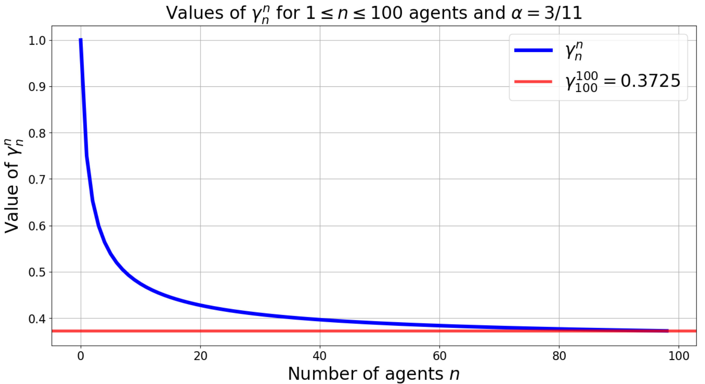
Values of were checked umerically by running a simple calculation program (see Figure 2 for values of for up to ). Since , there is still a lot of room left for improvement, so to maximize we will turn to the more complicated case .
A.4 Algorithm performance when
The proofs for are completely is analogous, and just require more technical work. We will need instead to use a different process . The following lemma is proved by induction.
Lemma A.10.
For agents, let be the following process: , and for ,
Assume . For every iteration of Algorithm 2 for agents, .
We state the analogue of Theorem A.1 for , proved in Appendix F (Corollary F.1).
Theorem A.3.
Let satisfy , and assume . For any constant , there exists such that for all it holds .
The doubling and main result also extend to , proved in Appendix G (Lemma G.2).
Lemma A.11.
Suppose that for some and it holds , for some value . If , then . Therefore, if , then .
Theorem A.4.
Let . Then , the remaining value after steps of Algorithm 2 for agents, satisfies for all .
Proof.
The proof is analogous to Theorem A.2. For , the value for which is . Then, by Corollary F.1, the gap between and will be at least , so we can take and have for the doubled process. Then, the doubling must satisfy , or . ∎

The values were checked directly via a computer program in Fig. 3.
Appendix B Different valuations
The algorithm for the general case, when valuations for agents are not necessarily the same, will have the same high-level structure. There will be iterations, and at iteration it picks some agent and allocates a bundle to this agent. There major difficulty that the algorithm needs to address in the multiple-agent case is the fact that different valuations result in different APS-partitions, which can be have problematic overlaps between each other. So, if say bundle is acceptable to agent , removing items of from APS-partitions of other agents may result in a significant loss of value. Therefore, the algorithm needs to ensure that not only every agents receives an acceptable bundle in the end, but also that giving a bundle to one agent keeps enough value in the APS-partitions of the agents that are still in the game.
For agent , let be her APS partition satisfying Lemma A.2. In the following sections, we will also assume that these APS partitions satisfy Claim A.1. This assumption is later removed in Appendix D, where we solve different instances with items of value at least using results obtained for the case when Claim A.1 does hold.
In our algorithm, each agent will keep track of their personal APS-partition, which is modified over the course of the algorithm. At every iteration, we remove some items from every bundle of the partition, while keeping the weights the same. We will need a similar terminology of filtered partition, used for the same-valuation case, extended to multiple agents.
Definition B.1.
For , consider agent with APS-partition , and suppose that this agent participates in the following high-level algorithm: there are iterations in total, and at every iteration , it removes some (possibly none) items from every bundle . We denote by the remaining items of at iteration , and let . We call a filtration of at iteration , and a filtered APS-partition. We will refer to as the remaining value of the filtered partition .
Throughout the algorithm, every agent maintains a filtration of . At some iteration , we may choose agent and allocate her an acceptable bundle . Unlike in Algorithm 2 before, the different-valuations algorithm will pick a bundle for agent probabilistically, using a distribution over subsets of the filtered partition . In order to construct this distribution, we use essentially the same ideas that were earlier described in Lemma A.3, Corollary A.1 and Lemma A.5. For completeness, we summarize these ideas in the following lemma.
Lemma B.1.
For , consider agent with valuation and APS-partition satisfying Lemma A.2, and let be some filtration of at iteration . For any such that satisfies , the following holds.
There exists a probability distribution over subsets of for , such that for every with it holds . In addition, for every item the probability to pick if we sample a random set satisfies , where
-
1.
if , then ;
-
2.
if and , then ;
-
3.
if and , then .
Proof.
We use Lemma A.3 on valuation and partition to distribute all bundles into classes for as follows: bundle belongs to if . As , and by Lemma A.2 there are no sets of value greater than , we will only have bundles of classes , where for every it holds . We denote for clarity, and proceed to construct using Lemma A.3.
Let , and let be defined accordingly as sums of weights of sets in corresponding classes. Let
Let be a (multi)-collection of sets, initially . For every with we check which of the -classes it belongs to.
-
•
If , we do nothing, effectively setting .
-
•
If , add a copy of into , and assign it probability .
-
•
If , let be sub-bundles of constructed as in Lemma A.3. For every , add a copy of to , and assign it probability .
-
•
If , let be sub-bundles of constructed as in Lemma A.3. For every , add a copy of to , and assign it probability .
By construction, any with satisfies . By Lemma A.5, is a valid probability distribution over , and for any item it holds
Finally, by Claim A.2 and Corollary A.2, we can upper bound by , with corresponding values of for different of and (as stated in lemma). ∎
B.1 Algorithm description
The high-level description of the algorithm for different valuations is quite similar to the same-valuation case (Algorithm 2). The algorithm has iterations and maintains a set of active agents at iteration , i.e the agents that still have not been allocated a bundle. At each iteration , we pick some agent , construct a distribution as in Lemma B.1, sample a bundle at random and give the bundle to agent . Then, agent becomes inactive, i.e , and we move to iteration .
In order to succeed, the algorithm needs to ensure that for the next agent picked at iteration , the remaining value of the filtered partition is at least , i.e (with high probability), otherwise Lemma B.1 cannot be applied and we would not be able to choose an acceptable bundle for . One could try mimicking previous approach of Algorithm 2, which, having allocated to , creates out of by simply removing items of from all bundles , i.e . Unfortunately, doing so in the different valuation case may cause the remaining agents in lose a lot of value. For example, we could sample an acceptable bundle for , such that for some agent that remains active, removing items of from bundles will force . And, if APS-partitions of different agents have significant overlaps, i.e multiple bundles of one agent have huge intersections with many different bundles of the other agents, the probability to pick a “wrong” bundle and remove a lot of value from the other agents can be quite substantial.
To mitigate this issue, our algorithm will include the following additional steps:
-
•
Before any allocations, for every agent we scan the initial partition and identify bundles that other agents on average find very valuable — we will refer to such bundles as “dangerous”. Then, we create a filtered partition where every dangerous bundle is replaced with , while all the other bundles are untouched. This effectively “bans” the algorithm from allocating any subset of a dangerous -s to in the future. Indeed, when we construct a distribution from Lemma B.1, every subset will have , while the probabilities of other bundles are increased. We show that the total weight of the dangerous bundles w.r.t APS-partition of is small, thus the value of is still close to , i.e loses almost no value by ignoring the dangerous bundles.
-
•
After picking agent and allocating her an acceptable bundle , for every remaining agent the algorithm keeps removing items of from bundles only as long as the total loss inflicted to does not exceed some value , decided in advance. This procedure, referred to as “filtering”, creates out of . Note that from the perspective of agent , agent only “partially owns” the allocated bundle , as the filtering procedure intentionally keeps some of the intersections of with .
-
•
While the filtering procedure guarantees that for every the total loss inflicted to is at most , at the same time it creates conflicts. It is now possible that at the future iteration, when agent is picked, the algorithm allocates her an acceptable bundle such that , i.e we allocate several items twice. To fix this, the algorithm “steals” the intersection from already allocated agent , and instead gives it to the currently picked agent , so that receives the bundle fully (at least for now). We will show that 1) if the filtering procedure removes items of from bundles in a specific way, then will not lose much value from stealing items of , and 2) since the filtered partition of agent did not have any dangerous bundles, then the number of agents that can potentially steal items from in the future is small.
With the steps above implemented, we guarantee that for every iteration and for every still active agent , the value loss is at most . Suppose that agents do not lose much value by removing dangerous bundles and having some of their items stolen in the future. Then, as long as for every iteration and agent picked at this iteration, the bundle picked for is acceptable, the algorithm succeeds. Note that by construction, if at iteration one can make the distribution from Lemma B.1, then a bundle sampled from this distribution is guaranteed to be acceptable for , i.e have . The only prerequisite is actually being able to construct , which by Lemma B.1 requires the remaining value of agent , , satisfy . As stated, by removing dangerous bundles agents do not lose a lot of value, so one can hope that for every we have , and the agent picked first, , gets an acceptable bundle. However, it is not clear whether the same will be true for agents picked at iterations , especially after removing items and updating the filtered partitions. For the algorithm to succeed it needs to assure that for every iteration and agent picked at some point in the future, the remaining value is at least .
We claim that this can be achieved if the agent chosen at iteration is exactly the agent with the largest remaining value . We show that if agents are is chosen this way at every iteration, over the course of the algorithm with high probability every agent keeps her remaining value at least , as long as the value loss is sufficiently small.
We are now ready to give a complete description of the algorithm for the different valuations case. First, we formally define what does it mean for a bundle to be “dangerous”.
Definition B.2.
Suppose that for every , APS-partition of agent satisfies Lemma A.2. For every set and agent , let
be the value lost by if we remove the items of the set from all bundles of the partition . Additionally, for every set and agent , let
be the total value lost by all agents, except for , if we remove items of from the their partitions.
We will pick some large value (say, of order ) in advance, and say that a bundle of agent is dangerous if . The algorithm for different valuations is presented in Algorithm 3 and Algorithm 4.
We will prove the following theorem about the performance of Algorithm 3.
Theorem B.1.
Let be some value in the segment , where is the solution to
There exists such that for all , the following holds: there exist values of such that after running Algorithm 3 on agents with APS-partitions satisfying Lemma A.2, with probability at least for every agent it holds .
B.2 Analysis of the algorithm
To prove Theorem B.1, we will analyze the performance of Algorithm 3 step by step. First, we will show the deterministic guarantees, specifically regarding the value loss of dangerous bundles and the filtering procedure of Algorithm 4. We start with a simple observation that at every iteration, the amount of value lost by agents is at most .
Lemma B.2.
For every and every agent that remains active after iteration of Algorithm 3, it holds that .
Proof.
Fix and . Since for every it holds , . Next, let be the agent picked at iteration of Algorithm 3, and let be the initially assigned bundle. In order to obtain from , the algorithm applies filtering procedure (Algorithm 4) to and set : set is sorted in decreasing order of , the value of the intersection of for agent . Then, Algorithm 4 removes items of only from sets for , i.e , where satisfies , and for all other , . By Lemma A.2, valuation acts like an additive function on all , so the lemma follows from for all and the definition . ∎
Next, before Algorithm 3 starts allocating bundles, for every agent it creates a filtered partition by effectively removing all dangerous bundles . That is, if has for the value , then , and otherwise . We will show that if is large enough, then the total weight of dangerous bundles of is small. As a corollary, removing all dangerous bundles from inflicts a very small loss of value, so , the value of , will still be almost .
Claim B.1.
For every and every agent , the amount of value lost by removing all such that is small. More specifically,
Proof.
By Lemma A.2, for all valuation acts like an additive function on subsets of , and also . Then, expanding the definition of and re-arranging summands,
Now, it is easy to see that for any number ,
The lemma follows by for all . ∎
Finally, we show that for every agent , the amount of value may lose from stealing items is small. We do so by analyzing the filtering procedure of Algorithm 4. First, we observe that the number of agents picked after that may potentially steal items from is small, as long as there are no dangerous items. Second, we prove that if some other agent ends up stealing items from , then from the perspective of the stolen value is not too large. We do so by noting that with respect to , the average value of intersection of the bundle picked for and the remaining bundles of must be small, and that by construction of Algorithm 4 agent can steal only lower valued intersections of . As a result, the value of the stolen intersection cannot be too large, and does not lose much value to . Combining these two observations together gives us the desired.
Claim B.2.
For , let be the bundle initially assigned to agent by Algorithm 3 at the iteration when was picked. Then , the final bundle of agent , satisfies
Proof.
Suppose that agent was picked at iteration . For every , denote by the bundle Algorithm 3 initially gave to agent at a future iteration when was picked. By construction, the final bundle that agent gets is exactly
Then, by subadditivity of ,
Fix some , and consider the filtering procedure, Algorithm 4, applied to agent at step . Let be sorted in decreasing order of , the value of the intersection of for agent . In addition, let be the largest number such that , i.e the total value of intersections of with bundles from up to is at most . There are two cases to consider.
First: . In this case, . That is, the total value the items in that are still remaining in the partition is at most . Then, for every it would hold that , i.e the filtering procedure removes all items of from the bundles of agent ’s partition. But then, if is the bundle that Algorithm 3 initially gives to at one of the future iterations, it must hold that . Thus, agent does not lose any value from such agent .
Second: . In this case, by maximality of ,
Suppose that this particular copy of came from a bundle , then . On the other hand, it must be that , hence by construction . Then, the number of agents such that is at most .
Let be the bundle that Algorithm 3 initially gives to at one of the future iterations (after ), and suppose that this particular copy of came from a bundle (as in Lemma B.1), for some . There are two possible options.
-
1.
if , by construction . Since is picked after iteration , and . In this case, agent does not lose any value from agent .
-
2.
if , then by construction , so agent may lose some value from agent , as filtering procedure does not remove items of from .
Suppose that . Then, for every it holds that . Therefore,
Observe that by maximality of it must holds . Indeed, if the opposite is true, as by Lemma A.2 for every we have ,
By Lemma A.2, for every it holds that , so adding to the sum above would increase it by at most , implying that is not maximal.
Now, since , by Lemma A.2 , furthermore, valuation acts like an additive function on . It follows that
Combining all the inequalities together, we get that if , the corresponding bundle of agent satisfies
As a result, if agent picks a bundle such that , then and hence does not steal anything from agent . On the other hand, if , agent loses at most value from agent , as shown above. Note that every agent who steals something from can steal only once, as they pick a single bundle . And, as we proved earlier, the number of such agents with is at most . Thus,
∎
Claim B.2 tells us the following: if for every agent the initially assigned bundle had value , then after Algorithm 3 finishes, agent would still have a bundle of value at least . If, for example, we pick and , then each agent would receive value at least . So, as mentioned earlier, in order to prove Theorem B.1 we need to guarantee that for every agent and every , if was picked by Algorithm 3 at iteration , it is possible to construct the distribution from Lemma B.1. That is, to show that with high probability, for every agent and iteration , if then the remaining value . This will be the main focus of the next section, where we prove the following theorem.
Theorem B.2.
Let be some value in the segment , where is defined in Theorem B.1. There exists such that for all , the following holds: there exist values of such that if we run Algorithm 3 on agents with APS-partitions satisfying Lemma A.2, with probability at least for every agent and every , if it holds .
Appendix C Proof of Theorem B.2
Our proof will rely on the observation made earlier in Lemma A.4. We will restate it in an equivalent way, using the terminology of Lemma B.1.
Lemma C.1 (Lemma A.4 restated).
For , consider agent with valuation and APS-partition , satisfying Lemma A.2, and let be some filtration of at iteration , such that . Let be the distribution over subsets of for , and let be such that for all . Then
The main idea of the proof of Theorem B.2 is as follows. Consider iteration and agent picked by Algorithm 3 at this iteration. By Lemma B.1, the distribution possesses the following property: for every item , the probability for item to belong in the bundle is at most . Suppose for a moment that for every the probability is exactly . Then, as shown earlier in the proof of Lemma C.1 (Lemma A.4), for every agent that stays active after iteration , the expected value of would be exactly . That is, on average every remaining agent would lose exactly -fraction of their current value . Of course, in reality agents are not guaranteed to lose exactly -fraction, they may lose much more or much less value. However, we will show that with high probability, for every agent the remaining value at all iterations (until the agent is picked) behaves not much worse than as if the agent loses exactly -fraction. And, the sequence where each agent loses exactly -fraction or better is essentially the process that was considered for the same-valuation case in the earlier section.
C.1 Expected process
Fix some agent , we will track the value at different iterations until is picked by Algorithm 3. By Claim B.1, with the appropriately chosen the initial value is at least , and by Lemma B.2, at every iteration the value does not decrease by more than . We will show that with high probability, the sequence of values is not much worse than the sequence of “expected” values of , where the agent loses exactly -fraction of her value. First and foremost, we define a so-called “expected process” of agent , which is essentially a sequence of values that is always decreased exactly by the expected fraction.
Definition C.1.
For , let denote the agent that was picked at iteration of Algorithm 3, and let be the smallest possible number such that for every item , . For agent , let be the following process: and for ,
We will show that if the maximum value and the variance of for various is bounded, then with high probability the expected process essentially serves as a lower bound to the sequence of values .
Theorem C.1.
Fix some , and let be some agent that remains active after iteration of Algorithm 3. For , let , and let be the smallest -algebra for random variables , i.e minimal -algebra w.r.t values for agents . Suppose that
for some . Then, for any ,
where .
The idea of the proof is the following. Suppose that Algorithm 3 picks agent at iteration . Then, by definition exactly. On the other hand, since is an upper bound on the probability , by Lemma C.1 in expectation the value of is at least . Then, the difference in expectation is at most . Note that if , then is at most . That is, when the value of the process is above the value of , the difference is shrinking in expectation. Therefore, at iterations when , the difference behaves like a super-martingale. So, to prove that does not exceed by more than , we can consider the iterations where is above and apply concentration inequalities for super-martingales.
Proof of Theorem C.1.
We will consider the sequence as a probabilistic process , where for all we set . For integer , define the stopping time
i.e the first iteration of after (and including) at which the process goes below .
Lemma C.2.
For integer , let be a stopped sub-process of which starts at time and stops at time . That is,
Then, for every , the process is a super-martingale.
Proof.
Recall that a sequence of random variables is called a (discrete time) super-martingale if for every time it holds
Observe that the process has a strong Markov property, for every , the values of and depend only on and on agents that are active in the beginning of iteration of the algorithm. Then, the process is a valid random process that depends only on and corresponds to a sub-process of starting from time onward. Consequently, the process is a valid random process that corresponds to stopped at time , i.e after time , this process remains constant equal to .
Now, for , let denote the agent that was picked at iteration of Algorithm 3, and let be the smallest possible number such that for every item , . By definition, for all we have , and by Lemma C.1, . Hence, for every
Then, it must hold for every that . Indeed,
-
•
if , then and the process has already stopped, so ;
-
•
if , then , and hence and , implying
Finally, as for any , we get that the process is a super-martingale. ∎
Suppose that for the given it holds . Then, it must also hold that . Indeed, as and by Lemma B.2, , then
Let be the smallest integer such that for every it holds , not that for such either or . In other words, is the start of the segment where for every the value stays non-negative. Since , such must exist.
Note that for this , it must hold that . Indeed, by the choice of , either and , or and . Since and by Lemma B.2, , if one had then
leading to a contradiction. Therefore, , and
Consider the stopped sub-process which starts at time and stops at time . By the choice of it holds that and and , so for every we have , and
We will use the following bound by [PIN94] on the deviation probabilities of super-martingales.
Theorem C.2 ([PIN94], theorem 8.2).
For a given , let be a real-valued super-martingale with respect to filtration of -algebras. Suppose that
for some . Then, for any ,
where .
As shown in Lemma C.2, is a super-martingale, with respect to filtration where for the -algebra is equal to of the process . Then, under the conditions on given by the statement of the theorem, we have
and
so by applying Theorem C.2 to and we obtain the bound
∎
In order to apply Theorem C.1, we need to upper bound the difference , as well as the sum of variances . This is the focus of the next two lemmas.
Lemma C.3.
Fix some and . For , let , and let be the smallest -algebra for random variables . For any :
Proof.
Lemma C.4.
Fix some and . For , let , and let be the smallest -algebra for random variables . For any :
Proof.
Observe that
By Lemma C.3, . Furthermore, the proof of Lemma C.3 implies that
hence
Therefore, using ,
To bound , consider the function for an arbitrary random variable distributed on the segment . Since is convex, it holds that
But then, the variance is at most
Note that is a non-negative random variable with expectation at most , and maximum value at most (by Lemma B.2). Then, is at most
It follows that
and thus
Using the fact that always, we obtain the final bound
∎
One could combine Theorem C.1, Lemma C.3 and Lemma C.4, we get the following bound: if is some agent that remains active after iteration of Algorithm 3, then for any
| (2) |
where is the smallest -algebra for random variables and , . The issue with such a bound is that the values of for are random variables themselves, and depend on , the filtered partition of the agent picked at corresponding iteration. As a result, the process is also a random process, so the bound obtained in Eq. 2 just by itself does not allow us to definitely conclude that the value of is at least , one would also need to bound the process first, as well as all the values of for . Instead, we would like to replace with some deterministic process, similar to what we did in the same-valuation case (Lemma A.7).
Consider Algorithm 3 and iteration , and for simplicity we assume that . Then, according to Lemma B.1, we can upper bound the value by
By construction, agent picked at iteration had the largest value . But then, and
Suppose now that for some . Then,
| (3) |
Note that the latter expression is very similar to the original process that we used in the same-valuation case, and it provides a lower bound on in terms of . Then, intuitively, if for all the lower bound holds, then the random process should be lower bounded by the deterministic process which matches the expression in Eq. 3 exactly. And, if is close to , and the deviation is small, then this deterministic process should be close to the original , which in turn was proven to be at least for any constant .
We will first cover a simpler case of and present a complete proof for this range of . The case of uses exactly the same ideas, but is a bit more involving technically and more formula-heavy, and we will cover it in the next subsection.
C.2 Proof of Theorem B.2 for
We will generalize the process used in the same valuation case from Appendix A, allowing the starting point to be some , as well as introducing an error inside the step-size. We will call the new process .
Definition C.2.
For agents, , and , let be the following process: and for ,
We will show that if for all the expected process lower bounds (up to an -error), then the deterministic process also lower bounds up to an -error.
Claim C.1.
For , let be some agent that remains active after iteration of Algorithm 3. For , let be the following event:
Under the event , it holds for all that .
Proof.
It suffices to show that for all it holds . We prove this via induction on . By definition, . Next, suppose that for all it holds . We show that .
For , let denote the agent that was picked at iteration . Recall that is the smallest possible number such that for every item , . By Lemma B.1,
Then, by definition of ,
Note that since , it must hold for every that , as otherwise agent would have been picked at step . Then, it holds for every that
Suppose that event holds, then for all it holds , and
Finally, it holds by induction that . Then, at step :
It follows that under the event , for all it holds . ∎
The lower bound of Claim C.1 allows to obtain a concrete upper bound on the values of .
Corollary C.1.
For , let denote the agent that was picked at iteration of Algorithm 3. For any , under the event it holds for every that .
Before making use of this upper bound, we will describe the main idea of the rest of the proof. Let be the agent picked at iteration . Let satisfy . Suppose that, for some value of and functions and we have . Then, by Claim C.1 under the event it holds — the desired lower bound in Theorem B.2. So, to prove Theorem B.2 it suffices to show that for large enough, with the appropriate choice of and , the event occurs with probability at least . Then, taking union bound over all iterations for a fixed agent , and after that over all agents , gives the desired probability of .
The lower bound for large will also be crucial in proving that the event happens with high probability, since this lower bound by Corollary C.1 implies that under the event for any it holds . As shown in Claim B.1, for every agent we have , hence (by induction) for every , . So, it suffices to prove that for any there exists some large such that for all it holds . We prove this lower bound in the following theorem.
Theorem C.3.
Let , and let satisfy . For any , there exists such that for all it holds .
The proof is rather technical, and we refer the reader to Appendix E. With Theorem C.3 equipped, we are ready to show that the event for fixed and occurs with high probability. This is done via the law of total probability and repeatedly applying the bound of Theorem C.1.
Corollary C.2.
Let and satisfy . Let satisfy , and . Let be such that for all it holds . For a fixed and , let be the agent picked at iteration of Algorithm 3 for agents. Then,
where
Proof.
By definition of the event , for any
Then, by the law of total expectation,
By definition, , so . Next, in order to bound for , we use Theorem C.1:
where and are such that for , under
By Lemma C.3 and Lemma C.4 we have the following upper bounds:
and
Now, by Corollary C.1 under the event it holds
hence under the event we have upper bounds
and
Recall that by Claim B.1, for every agent we have . It is easy to see (via induction on as in Claim C.1) that for every we have a lower bound . Then, since , for these and agent it holds . So under the event we have
We pick these upper bounds as and respectively. Observe that in this case
Now, since for any , it holds for with that
hence
Since this bound holds for all , we have
This finishes the proof. ∎
Corollary C.2 allows us to show that for the choice and , if agent is picked at iteration of the algorithm, then . This will complete the proof of Theorem B.2. As a result, with high probability all iterations of Algorithm 3 will succeed, i.e it will able to construct a distribution and allocate an acceptable bundle for .
Corollary C.3.
Let and satisfy . For a fixed , let , and as functions of . There exists such that for all , running Algorithm 3 on agents, with probability at least for every agent and every iteration , if then .
Proof.
By Theorem C.3, for these values of there exists such that for all it holds . Fix some . For every and agent , by Claim C.1 under the event it holds that . As mentioned in the proof of Corollary C.2, Claim B.1 implies that , hence for this it holds under the event that . So, it suffices to show that the probability that there exists any agent and any iteration , such that but event does not occur, is small. By union bound,
By the choice of we have . So, by Corollary C.2, for every it holds
By the choice of , , hence by the choice of we get
We conclude that
∎
It is easy to see that Corollary C.3 directly implies Theorem B.2 for . We combine all the obtained bounds to prove the following theorem.
Theorem C.4.
For every , there exists , such that for all the following holds. For every fair allocation instance of indivisible goods to agents with XOS valuations and APS-partitions satisfying Lemma A.2 and Claim A.1, there exists an allocation algorithm that with probability produces an allocation where each agent receives at least -fraction of her APS.
Proof.
Let satisfy , and let . For some value , consider Algorithm 3 on with this value , note that as , there are no items of value over in any of APS-partitions, thus Lemma A.3 is applicable. We pick values and . By Corollary C.3, for there exists such that if , it holds with probability at least that for every agent and every iteration , if then .
As a result, if , with probability at least every iteration of Algorithm 3 on this instance will succeed. It follows that if the agent was picked at iteration and initially assigned a bundle , then . Hence, by Claim B.2
Since , there exists such that for all ,
But then for every agent we have . ∎
C.3
The proofs for are essentially the same as for the case , and differ only in minor technicalities. When , upper bounds on probabilities arising from Lemma B.1 vary depending on whether the agent ’s current value, , is above or below . Because of this, the definition of the deterministic process will also be adaptive.
Definition C.3.
For agents, , and , let be the following process: and for ,
-
•
if , then
-
•
if , then
With this definition of , we show that, as in Claim C.1 for , when we also have a lower bound on under the event .
Claim C.2.
For , let be some agent that remains active after iteration of Algorithm 3. For , let be the following event:
Under the event , it holds for all that .
Proof.
Once again, it suffices to show that for all , . We prove this via induction on , the equality holds by definition. Suppose now that for all it holds , we show that .
Observe that when , for any it holds
| (4) |
Therefore, using the upper bound on from Lemma B.1,
Similar to , when under the event it also holds that for all . Now each of the values can be above or below , and we will have to consider different cases. Note that if one value is above , by Eq. 4 we lower bound for “both cases”, as demonstrated above for . Then, depending on what is the value of the next variable in , we can pick the appropriate lower bound.
Repeating the same chain of inequalities: since ,
Since ,
Finally, by induction . Hence,
It follows that under , for all it holds . ∎
Corollary C.4.
For , let denote the agent that was picked at iteration of Algorithm 3. For any , under the event it holds for every that .
Proof.
As with , when we also need a lower bound of the form for every agent . The following theorem is the extension of Theorem C.3 to values .
Theorem C.5.
Let satisfy , and assume . For any , there exists such that for all it holds .
The proof is essentially the same as the proof of Theorem C.3, just a bit more technical. We refer the reader to Appendix F. Now, we can show that for fixed , the event occurs with high probability also for . The following statements are extensions of Corollary C.2 and Corollary C.3 to , and are proven analogously.
Corollary C.5.
Let satisfy , and assume . Let satisfy , and . Let be such that for all it holds . For a fixed and , let be the agent picked at iteration of Algorithm 3. Then,
where
Corollary C.6.
Let satisfy , and assume . For a fixed , let , and as functions of . There exists such that for all , running Algorithm 3 on agents, with probability at least for every agent and every iteration , if then .
Finally, we combine Corollary C.5 and Corollary C.6 to prove the analogue of Theorem C.4 for the case (picking , and for ).
Theorem C.6.
Let satisfy . For every , there exists , such that for all the following holds. For every fair allocation instance of indivisible goods to agents with XOS valuations and APS-partitions satisfying Lemma A.2 and Claim A.1, there exists an allocation algorithm that with probability produces an allocation where each agent receives at least -fraction of her APS.
Appendix D Big Items
For every agent and item , we say that item is big for if , and small for if . We have showed in previous sections that if all items are small for all agents, i.e Claim A.1 is satisfied, then there exists an allocation where each agent gets at least -APS for . In this section, we show how to get rid of the requirement of Claim A.1.
D.1 Properties of bipartite graph
Below we show that any bipartite graph with must satisfy one of the four structural conditions. Then, we consider the graph with , and , and prove that if satisfies one of these four conditions, there exists an -APS allocation for .
Lemma D.1.
Let and be arbitrary. For every bipartite graph with and , one of the following must hold.
-
1.
has a matching in which all of is matched.
-
2.
has a maximal matching with at most edges.
-
3.
There are partitions of and of with the following properties:
-
(a)
, and form a perfect matching which is maximal in ;
-
(b)
for every vertex we have .
-
(a)
-
4.
There are partitions of and of with the following properties:
-
(a)
, and form a perfect matching;
-
(b)
there are no edges between and and between and ;
-
(c)
;
-
(d)
for every subset of size there is a perfect matching between and .
-
(a)
Proof.
We will show that if items 1), 2), 3) do not hold, then 4) must hold.
We first prove that if 1), 2), 3) do not hold, there exists a set of size at least , such that every vertex has at least neighbors in . To see this, observe that
-
•
by 1), every maximal matching in has size , so is nonempty;
-
•
by 2), , thus ;
-
•
hence, by 3), for every maximal matching in there exists a vertex such that .
We will pick vertices into iteratively, starting with . Let be arbitrary maximal matching in , then there exists some vertex such that . We add to , and, if possible, extend to a maximal matching in , containing . Then, there exists some vertex such that . We add to and then, if possible, extend to a maximal matching containing , then take vertex and so on. We continue doing so until we no longer can find a maximal matching containing all .
Since at any point for every vertex it holds , it is always possible to perfectly match all current vertices of as long as , and therefore possible to obtain a maximal matching containing all . Thus, if at some point it is no longer possible to extend to a maximal matching, we must have . We then add to this all other remaining vertices with at least neighbors (if there are any).
Consider this , we have , and for all it holds . Denote , and , we have . We start forming sets and , initially all of them are empty.
Go over all vertices in arbitrary order, if is nonempty, take and match together, adding to and to . It is clear that in the end of this procedure, if some was unmatched, then , i.e there are no edges between and . We then add all unmatched vertices of to . Similarly, for every unmatched vertex there are no edges between and — there can’t be edges with by definition, and all neighbors of in have already been matched. We then add all unmatched vertices of to . In addition, as , we could not have matched more than vertices of , therefore we could not have matched more than vertices of . As a result, for every vertex there will be at least neighbors left in .
Consider the subgraph of on . We claim that there is no perfect matching between and . Suppose the contrary, then and together form a perfect matching which is maximal in . Indeed, by construction the only unmatched vertices would be and , and there are no edges between them. Now, take some vertex . By construction, , hence . At the same time, since is maximal, case 2) not holding implies that , so . Thus, all have . But then we find ourselves in case 3), which does not hold by assumption.
As a result, there is no perfect matching between and . Then, by Hall’s theorem there exists a subset such that satisfies . Since every vertex in has at least neighbors in , we have and .
Let , and . We go over all vertices in arbitrary order, and if is nonempty, take and match together, adding to and to . Similar to what we did before, in the end of this procedure all unmatched vertices of have no edges into , and we add them to . At the same time, all unmatched vertices of have no edges into , and we add them to . Since , the total number of matched vertices of both and cannot exceed . Note that for every vertex , contains exactly the vertices that have not been matched. Every vertex initially had at least neighbors in , and the total number of matched vertices of cannot exceed . Then, for every vertex there will be at least neighbors left in , hence .
Next, let contain all vertices such that . We lemma that . To estimate , consider the subgraph induced on . Every vertex in has degree at most , and every vertex not in has degree at most . Since and for every , , the total number of edges in this subgraph is at least , and , we have the following lower bound:
Let . Now, we go over all vertices in arbitrary order, and if is nonempty, take , and match together, adding to and to . In the end of the procedure, all unmatched vertices of have no edges into , and we add them to . Let denote the remaining vertices of , and . Clearly, . Since , then . Therefore, the number of matched vertices of satisfies . Furthermore, every vertex has lost at most neighbors, so . Finally, consider the remaining vertices . Observe that
Note that the vertices include all the vertices of that have been matched with , plus some additional vertices that remained unmatched. Then, and . And, since , each vertex has at least
neighbors left in . The last inequality uses .
We take and . To finish the proof, it remains to show that if has size , there exists a perfect matching between and . By construction for every it holds . At the same time, we showed above that every vertex has at least neighbors left in . Thus, in the subgraph induced on , every vertex has degree at least . The lemma follows from the fact that any bipartite graph where every vertex has degree at least has a perfect matching. ∎
D.2 Allocations for cases 1), 2), 3)
We first deal with cases 1) and 2), they are pretty straightforward.
Claim D.1.
Let satisfy . For every , there exists , such that for all the following holds.
Consider the graph with , and . If satisfies cases 1) or 2) of Lemma D.1, then there exists an allocation where each agent receives at least -fraction of her APS.
Proof.
Suppose that case 1) of Lemma D.1 holds for . Then, there exists a matching in such that every agent is matched with a unique item satisfying . So, we trivially get an -APS allocation.
Next, suppose that case 2) of Lemma D.1 holds for and . Let be the maximal matching in with at most edges. Recall Lemma A.1, which we restate it here for convenience:
Lemma D.2.
For any item and any valuation , .
For every edge of the matching , we give item to , then receives -fraction of her APS. By Lemma D.2, for all the remaining agents in the APS will not decrease after we remove all items and agents from . Since the matching was maximal, for every agent there are no big items remaining in . Furthermore, the number of remaining agents is at least .
As shown in Theorem C.6, there exists such that for all , every fair allocation instance with XOS agents and APS partitions satisfying Lemma A.2 and Claim A.1 has an -APS allocation. Then, if , we can apply Theorem C.6 to the agents , items and the corresponding APS partitions, and therefore get an -APS allocation for all agents of . ∎
Case 3) is quite more convoluted, we analyze it in the following lemma.
Lemma D.3.
Let , and consider the graph with , and . If satisfies case 3) of Lemma D.1, then there exists an allocation where each agent receives at least -fraction of her APS.
Proof.
Suppose that case 3) of Lemma D.1 holds for . Let and be the corresponding partitions, where form a perfect matching. Similarly to case 2), for every edge , we give item to , then receives -fraction of her APS. By Lemma D.2, for all the remaining agents in , the APS will not decrease after we removed all items and agents from . So, it remains to allocate the remaining items among agents .
For every agent , consider her APS partition , and let be the set of all bundles such that contains some big item (i.e ) that was allocated to someone in . In other words, if and , then . Denote . By construction, for every agent we have , so the total weight is at most . Indeed, for every item we have , and there are at most big items, so in the “worst” case each of the big item would have its own disjoint set of bundles containing it.
Note that since , there are at least allocated items that were small for agent . For convenience, we “pretend” that some of these small allocated items were actually “big”. Specifically, we go over small allocated items one by one, and for item we include the bundles of containing into . We do so until there are exactly “big” allocated items. Denote these “big” items by , and the remaining small items by . Note that .
Consider the bundles , by definition any contains no items from , and either lost no items from the allocation , or could have potentially lost some small items from . For every item , denote by the set of bundles that contain . In addition, denote by the subsets of containing bundles that lost respectively exactly , exactly and at least small items from . We say that two sets and are disjoint, if there are no such that or such that . Note that if all sets for are disjoint, then and .
Let be such that there are exactly disjoint sets for . Without loss of generality, let , and sets for are disjoint. Note that by definition, for every , non-disjoint set can contain only bundles . Indeed, if , there exists for such that and hence . It will be important that this set must contain at least one bundle from . We will use this observation to show that .
Suppose that there are disjoint sets such that there exists which lost at least items, i.e . The fact that these sets are disjoint implies that there must exist at least disjoint bundles . But then, since each of these bundles contains at least items from , we have , which is impossible.
As a result, there must be disjoint sets such that contain some . Without loss of generality, let these sets be . We lemma that any bundle belongs to exactly one of disjoint sets for . Indeed, as mentioned earlier, for every where , i.e is non-disjoint, we must have , and there must exist some such that . But then
As a corollary, for every agent that was not allocated, the total weight of the bundles in is at least . By definition for every we have , as each bundle could lose at most one small item. In order to allocate the remaining agents, we will use the approach developed in [GHS+22, FG25].
Without loss of generality, let . For every agent , let be a capped valuation function defined as , note that when is XOS, so is valuation . Let be the allocation of items among agents , such that agent receives bundle , and the welfare w.r.t -s is maximal. We lemma that for every agent , .
To see this, for a fixed agent consider its APS-partition for the original sets . We construct the following distribution over subsets of : for every bundle , let . Suppose that for we have . Then, sample a random bundle , and give the bundle instead, and to every other agent give bundle . Since is non-zero only if , we must have , so agent gained at least welfare. At the same time, for every item the probability that contains satisfies
because . Now, take some agent . Since her valuation acts like an additive function on , in expectation agent lost at most
But then in expectation the total value lost by all other agents is at most
implying that there exists a choice of such that the allocation will achieve strictly larger welfare than , leading to a contradiction. Hence, for a maximal welfare , for every we must have . Finally, , so , which finishes the proof. ∎
D.3 Allocation for case 4): agents and
Case 4 is the hardest one to deal with, it corresponds to the instance where the vast majority of agents agree which items are big and which items are small, while a small fraction of agents do not have any big items at all. In order to get an -APS allocation for this case, we design a new algorithm, inspired by both Algorithm 2 and Algorithm 3.
Suppose that case 4) of Lemma D.1 holds for and some , denote . Let and be the corresponding partitions. Let be the perfect matching between and . Similarly to cases 2) and 3), for every edge , we give item to , then receives -fraction of her APS. By Lemma D.2, for all the remaining agents in the APS will not decrease after we remove all items and agents from . So, it remains to allocate the remaining items among agents .
By construction, items are small for both agents in and in , while items are small only for agents in . Since , the set contains at least agents, and there are at most agents in . Since is large, we cannot simply give big items to as many agents in as possible and then try to allocate the leftovers of and using only small items of , using for example the algorithm of Theorem C.6. First, Theorem C.6 holds only when applied to at least agents, while we will have less than agents left. Second, if is allocated first, there is no guarantee that for the leftovers of and the remaining items will provide enough APS-value, if anything, the vast majority of the APS-value will be lost.
Instead, we will allocate agents of first. Since for all items of are small, one may try and apply Theorem C.6 and Algorithm 3 to agents . However, , so if we assume that are the only agents participating in Algorithm 3 and consider their APS-partitions of items among only agents , the algorithm will not succeed. The issue is that when there are substantially less than total agents, for every step of Algorithm 3 the probabilities for distributions will be too large, thus agents that remain active after step will lose a lot of their APS-value , forcing it to drop below very fast.
Another shortcoming of the approach suggested above is that if we allow agents in Algorithm 3 to pick items from , agents can take almost all items of just for themselves, and then we will not be able to match with the remainder of . This is due to the fact that all items of are small for all agents of , and Algorithm 3 gives no upper bound on the number of items each allocated agent may get.
To mitigate these issues, we modify Algorithm 3 and run it on all agents together, and consider their APS-partitions of items among all agents . However, we will force the algorithm to pick and allocate only agents from at every step, and use only items from , and run it until all agents of are allocated. One may ask whether there is enough value left for agents if we restrict them only to items from , and also whether after we allocate , there will be enough value left for agents from the remaining items of . To answer these questions, we first observe that agents , the vast majority of APS-value must come from the items of , while agents possesses an APS partition of items among agents of value at least .
Claim D.2.
-
1.
For agent , let be her APS partition. Then
-
2.
For every agent , there exists an APS-partition of only items among agents such that its value satisfies
Proof.
By construction, every item is small for every agent . Therefore, by deleting from every bundle the agent loses at most value. And, as , removing all from bundles of will decrease the APS-value of by at most .
Next, for , consider the initial APS-partition of agent over all agents and all items , its value is at least . By construction of , there exists a matching such that and . Then, we can apply Lemma D.2 to all agents of and their matched items of , repeatedly removing pairs . By Lemma D.2, for all the remaining agents, including , their APS will not decrease. So, for the obtained APS-partition of the remaining items, i.e , among the remaining agents, including , we will have . ∎
For every agent , we the APS-partition from Claim D.2, without loss of generality we can assume that it satisfies Lemma A.2. Then, for every we would have .
Since the algorithm only picks agents from , values of for agents will not affect its performance at all. Because of this, we will filter-out dangerous bundles, as well as ensure that the APS-value decrease at every step is bounded, only for agents from . In essence, while agents from do participate in the algorithm, they play an “observant” role and just lose APS-value at every step from allocations. That is, every time agent is given some bundle, say , by the algorithm, for the algorithm completely removes the items of from ’s APS partition. The full description of the algorithm is given below.
We will prove the following theorem about the performance of Algorithm 5.
Theorem D.1.
Let satisfy . For every there exists , such that for all the following holds: after running Algorithm 5, with probability at least
-
1.
every agent receives a bundle satisfying ;
-
2.
remaining APS-values for agents satisfy
Given this theorem, we then can do similar trick as in Theorem C.4 and Theorem C.6: run Algorithm 5 w.r.t value . Since every agent has only items of value less than in their APS partition, these APS partitions satisfy Lemma A.2 and Assumption for item value for . Then, Lemma B.1 applies for , and the Algorithm 5 will try to obtain an -allocation for agents in . Taking large enough so that will guarantee that . At the same time, agents will have
Thus we obtain the following corollary.
Corollary D.1.
Let satisfy . For every there exists , such that for all the following holds: there exists an allocation of some of the items among agents such that
-
1.
every agent receives a bundle satisfying ;
-
2.
values for agents satisfy
Proof of Theorem D.1.
For , let denote the agent that was picked at iteration of Algorithm 5, and let be the smallest possible number such that for every item , . Once again, for every we consider the process defined as and for , . Consider the deterministic process for some value .
Claim D.3.
For , let be some agent from that remains active after iteration of Algorithm 5. For , let be the following event:
Under the event , it holds for all that . Furthermore, if agent was picked at iteration of Algorithm 5, under the event for every it holds
Proof.
Follows directly from Claim C.2 and Corollary C.4 by observing that all was the largest among for agents that were still active, i.e . ∎
In order to prove Theorem D.1, we need to show that Algorithm 5 at every iteration manages to successfully construct distribution . As before, this requires showing that 1) for every , process is at least (provided that is large enough), and 2) for every agent and every iteration of Algorithm 5, the probability that the event does not occur is small.
Note that for every values at all iterations are affected only by other for . In addition, by Claim D.2 we have for all . Now, consider the simplified statement of Corollary F.1.
Theorem D.2 (Corollary F.1 restated).
For , let . Consider the process for this , and some , and take integer such that . Then, if satisfy
| (5) |
In our case, , where satisfies . For these values of parameters and , the lefthand side expression of Eq. 5 is at least . Next, as , we pick in Theorem D.2. Finally, for the process we pick and . Then, the righthand side of Eq. 5 is at most
Choosing small enough constant so that , and picking such that guarantees that for large enough value of (i.e, large enough ), we have for all .
It follows that, similar to Corollary C.5 and Corollary C.6, one can pick values of in Algorithm 5 and choose such that and with probability at least for every agent and iteration , if then . But then it follows directly from the proof of Corollary C.6 and Claim B.1 that after running Algorithm 5, every agent receives a bundle such that .
Now we show that with probability at least , agents must satisfy . To see this, fix some and consider the expectation over distributions . By Lemma A.4, for every we have
Since , by Claim D.3 with probability at least for every it holds
for our choice of . Since is large enough, we have for every picked , thus
where the last inequality follows from and . Then, by Markov inequality, with probability at least it holds
It follows by the law of total probability that with probability at least it holds
∎
D.4 Allocation for case 4): agents
For every agent , let be the APS partition of only items among agents from Claim D.2, satisfying Lemma A.2. We showed in Theorem D.1 and Corollary D.1 that there exists an allocation of items among agents with the following properties:
-
•
every agent receives a bundle of value at least -APS;
-
•
values for agents satisfy
We will now focus on allocating agents . By construction, every subset of size forms a perfect matching with . Hence, it is sufficient to allocate arbitrary agents of using the items of , and then use the matching to give a single personal big item to each of the remaining agents of .
We will do this using a generalization of our initially presented approach for the case of same-valuation agents, specifically the greedy algorithm Algorithm 2, to the case of agents with different valuations. We will abuse notation and let denote the filtered APS-partition of agent , obtained from the original after Algorithm 5 (with the property on average above).
Denote , so , and let be the smallest constant satisfying . Our algorithm will run for iterations, and at every iteration we maintain a set of agents that are still active, as well as total values of their filtered APS partitions over items . For iteration and any set , denote
At every iteration , we pick an active agent with largest value , and then greedily choose for her bundle that maximizes the average value . We allocate to and set . We run this algorithm until exactly agents are allocated, and then give out single big items to the remaining agents, similar to what we did in previous cases 1), 2) and 3). The full description of this greedy-average algorithm, Algorithm 6, is given below.
We will now analyze the performance of Algorithm 6. It is going to be quite similar to the analysis of Algorithm 2, with additional caveats. First, we are going to define a new special process .
Definition D.1.
Let be the following process: , and for ,
where .
Similarly to the case of same valuations covered in Lemma A.7 and Lemma A.10, we use to lower bound the average remaining value of active agents . Then, if the value stays large enough after iterations of Algorithm 6, it guarantees that all iterations will succeed.
Theorem D.3.
For every iteration it holds
Proof.
We will use induction to prove the following claim. Define the process as follows , and for all ,
The base case follows trivially by definition of and . Suppose that the lower bound holds for all , we want to show it for .
Let denote the agent that was picked at iteration of the algorithm. It follows from Lemma A.4, Corollary A.1 and Corollary A.2 that the chosen bundle from satisfies
where if , then , and if , then . Since has the largest among , applying averaging and using the inductive assumption yields us . Hence, using inductive step,
Since , and , the inequality above implies
Now, it is easy to see (e.g via induction) that the recursive process satisfies . Furthermore, for every we have . Then, since and , we obtain that for every ,
Next, and imply that . To see this, we use a proof similar to Claim C.2 and utilize the upper bound on above, replacing first with and then with . Thus, induction step is also proved, and the lemma follows. ∎
Recall that Lemma A.3 and Corollary A.1 succeed to pick an acceptable from for agent only if . So, to prove that Algorithm 6 indeed works, by Theorem D.3 it suffices to show that for every we have .
Let be some constant (dependent on ) that satisfies , and will be defined later. First, we use Theorem D.2 and show that there exists such that when is large enough, it holds . Recall that by definition, . We substitute values , , , same and into Theorem D.2, and obtain that if
| (6) |
As shown in the proof of Theorem C.5, for values of the lefthand side of Eq. 6 is at least . Then, we can pick sufficiently small and the largest value for this so that the righthand side of Eq. 6 without part is strictly less than the lefthand side, we will get for sufficiently large .
However, , so the bound on that works only when is large is not good enough! Fortunately, the bound actually holds for all . This is due to the fact that even though process loses an additional term of , when compared with the original process for the same valuation case, this being a fixed constant allows us to apply the doubling procedure also to ! Specifically, we prove the following lemma in Appendix G (Lemma G.2):
Lemma D.4.
Suppose that for some and it holds , for some value . If
where is constant, then .
If is large enough for Eq. 6 to hold by itself, it already holds . Otherwise, we can find large enough such that , and for large enough choice of we would have . Then by Corollary A.3 we could reduce to and so on. Note that the smaller is, the smaller we could take the constant and hence the larger we could take the constant . Then, we continue doing the doubling for all values of until some constant, and from there the values of are checked numerically. Hence, for every given one can pick small enough values , and to guarantee doubling for any any target number of values to check.
Appendix E Lower bound on for
Recall the definition of process for .
Definition E.1.
For agents, , and , let be the following process: , and for ,
In this section, we prove Theorem C.3, restated below. Note that the claim of (Theorem A.1) is a special case of this theorem with .
Theorem E.1.
For let satisfy . For any constant and any , there exists such that for all and all it holds .
First, we consider a process for arbitrary and , and obtain a lower bound on the number of iterations required for such process, having started at value , to drop below value . To do so, we break the segment into many epochs of the form w.r.t current value of . Then, we estimate the minimum number of iterations the process spends in each epoch, and determine for which values of the total number of estimated iterations over all epochs exceeds some .
Lemma E.1.
Consider the process for some , and . For , let be the largest integer such that , and let be the smallest integer such that at the beginning of iteration it holds . Then
-
1.
For any and any integer , the minimum number of steps of to reach is
-
2.
For any such that , the number of steps of the process after the iteration for the value to go below satisfies
-
3.
For any and any integer , it holds that if
Proof.
To prove 1), first assume that is an integer. Divide the segment into smaller sub-segments of the form where . Note that by definition, for any it holds . In particular,
Therefore,
Since , we get
If is not an integer, we consider a segment , divide it into sub-segments and repeat the process above. This gives us
We finish the proof by observing
Next, for 2), observe that by definition of , for every integer it holds . Then, by definition of the process , for every such we have
Applying the inequality above repeatedly, we get
implying
Now, since for all it holds , we have
To see 3), note that implies that at iteration of the process we have . Combining the expression for from 1) and lower bound on from 2) completes the proof. ∎
Using the lower bound on the number of iterations required for to stay above after iterations, we can get a necessary condition on and for the inequality to hold. To do so, we take the inequality of 3) from Lemma E.1 and perform multiple equivalent transformations.
Theorem E.2.
For , let . Consider the process for this , and some , and take integer such that . If numbers satisfy
| (7) |
then the value of the process at iteration satisfies .
Proof.
From Lemma E.1 we know that if integers with are such that
| (8) |
Consider the expression for , derived in Lemma E.1, with and :
We have . Observe that
Hence, if
then Eq. 8 holds. Since , we have
Additionally, since
it is easy to see that Eq. 8 also follows from inequality
Note that for values of , the function is non-decreasing:
Therefore, it holds
where the last inequality follows from and shrinking the integration domain.
The proof of Theorem E.1 follows directly from the following refinement of Theorem E.2.
Corollary E.1.
For , let . Consider the process for this , and some , and take integer such that . Then, if satisfy
| (9) |
Proof.
Consider the expression obtained in Theorem E.2 for some and instead of . Observe that
Since , then and . In addition, when ,
Finally, as , we have
Combining all of the above and noting , Theorem E.2 holds if satisfy
∎
Proof of Theorem E.1.
First, observe that for all , as long as , the lefthand side of Eq. 9 in Corollary E.1 is a decreasing function of . Indeed, the derivative of is , which is non-positive for all . Then, if is a solution to , for any constant it holds for that .
At the same time, when the righthand side of Eq. 9 in Corollary E.1 is at least . Since , both and are of order , and taking any integer in
makes the expression into a decreasing function of , specifically of order . But then, with this value , if , when the righthand side of Eq. 9 converges to as . Thus, for inequality to be satisfied for all it suffices to take large enough such that the righthand side of Eq. 9 with is at most . Since , such must exist. ∎
Appendix F Lower bound on for
Recall the definition of the process for .
Definition F.1.
For agents, , and , let be the following process: , and for ,
In this section, we prove Theorem C.5, restated below. Similarly to how it was with , the claim for the same-valuation case (Theorem A.3) follows by setting .
Theorem F.1.
Let satisfy , and assume . For any constant and any , there exists such that for all and any it holds .
The structure of the proof is essentially the same as in Lemma E.1, Theorem E.2 and Corollary E.1 for the case , with only difference that now one has to consider regimes above and below . As before, we first consider arbitrary and , and obtain a necessary condition on so that .
Theorem F.2.
For , let . Consider the process for this , and some , and take integer such that . Then, if satisfy
| (10) |
Proof.
By the first item of Lemma E.1 (which holds for all values of ), the minimum number of steps of to reach is
Observe that
It is easy to see that
Consider for . For this range of values, as was done in Lemma E.1,
implying
Similarly, consider for . For this range of values it holds
implying
As a result,
Now, we substitute and into and .
As was done in Theorem E.2, we observe that
and
Combining all of the above with , we get that if satisfy
Next,
so we get an equivalent condition (after dividing by )
Next, since both and are decreasing functions of on respective ranges, and by shrinking the integration domain, we have
Taking the integrals:
and
Now, and and , so
and
So, we have an equivalent condition on :
∎
Similarly to Corollary E.1, we obtain a refinement of Theorem F.2 for and .
Corollary F.1.
For , let . Consider the process for this , and some , and take integer such that . Then, if satisfy
| (11) |
Proof.
First, replacing and using and , from Eq. 10 we get a condition for any :
Next, we substitute instead of and make the following observations:
and
We conclude that if satisfy
∎
Proof of Theorem C.5.
First, observe that for all , as long as , the lefthand side of Eq. 11 in Corollary F.1 is a decreasing function of . Indeed, the derivative of is , which is non-positive for all . Then, if is a solution to
| (12) |
for any constant it holds for that is strictly greater than .
Note that, unlike in Theorem E.1 and , when there is an upper bound on the values of for which there would exist such a solution to Eq. 12. Specifically, one could increase the value of until the only viable solution is exactly . This largest possible then must satisfy
which gives us maximum possible . Thus, if and is such that , it holds for that is a constant greater than .
At the same time, when the righthand side of Eq. 11 in Corollary F.1 is at least . Since , both and are of order , and taking any integer in
makes the expression into a decreasing function of , specifically of order . Taking this value of with when makes the righthand side of Eq. 11 converge to as . Thus, for inequality to be satisfied for all it suffices to take large enough such that the righthand side of Eq. 11 with is at most with . Since the latter expression is strictly greater than , such must exist. ∎
Appendix G Doubling
First, we prove the doubling lemma for the case .
Lemma G.1.
Assume that and is constant, and consider the following process : , and for all ,
Suppose that for some and it holds for some value . If
then .
Proof.
By definition of the process , if then
and
To prove the lemma, it remains to determine for which values of the expression above is at most . Since , we have by definition
Thus, to prove , it suffices to show that
Opening up the parenthesis, we get
Removing from each side, diving by and multiplying by gives
Adding to each side and multiplying by (assuming it is positive) gives
The last inequality always holds. As mentioned, this is an equivalent transformation only if
Solving the equation for , we have
∎
The proof for the case is completely analogous, the only major difference is that we have to consider cases of whether are above or below , which makes the proof quite longer (though technically as simple).
Lemma G.2.
Let satisfy , and assume and is constant. Consider the following process : , and for all ,
Suppose that for some and it holds , for some value . If
then .
Proof.
There are four cases to consider, depending on whether are above or below . First case is , note that we also have . Then, by definition
and
Once again, we would like to determine for which values of the expression above is at most . By definition,
Thus, to prove , it suffices to show that
Opening up the parenthesis,
Removing from each side, dividing by and multiplying by gives
Adding to each side and multiplying by (assuming it is positive):
The last inequality always holds. As mentioned, this is an equivalent transformation only if
Note that by assumption, . Then, , and the inequality above holds if . Since , for all . So, the expression above is always positive for our ranges of and .
Second case is while , note that still . By definition,
and,
as well as
Thus, to prove , it suffices to show that
Opening up the parenthesis and combining like terms,
Multiplying everything by , we have
Multiplying by (assuming it is positive):
which is equivalent to
which holds if and only if
Since and , it holds
so it suffices to show that
which is always true for . So, the inequality holds as long as
Once again, since , we have , and the inequality above holds if . As , inequality holds if , which is true for .
The third case is , while , and in this case . Observe that when , for any we have
Then, by definition
which would be a formula for if . So, we can reduce the case of and to the final case, where all . Once again, by definition
and
as well as
Thus, to prove , it suffices to show that
Opening up the parenthesis and combining like terms,
Diving everything by and multiplying , we get
Multiplying by (assuming it is positive):
The last inequality always holds. As mentioned, this is an equivalent transformation only if
Solving the equation for , we have
∎