Mask2Cause: Causal Discovery via Adjacency Constrained Causal Attention ††thanks: Code is publicly available at: https://github.com/omar826/Mask2Cause
Abstract
Leveraging deep learning for causal discovery in time series remains challenging because existing neural methods predominantly rely on component-wise architectures that fail to capture shared system dynamics, or employ decoupled post-hoc graph extraction that risks overfitting to spurious correlations. We propose Mask2Cause, an end-to-end framework that recovers the underlying causal graph directly during the forecasting forward pass. Our approach introduces an Inverted Variable Embedding and an Adjacency-Constrained Masked Attention mechanism, trained with homoscedastic or heteroscedastic objectives to capture causal influences in both mean and variance. Empirical results on diverse benchmarks, from synthetic chaotic dynamics to realistic biological simulations, demonstrate state-of-the-art causal discovery with significantly reduced parameter complexity compared to standard baselines. We further show that inferred causal structures can be used to reduce parameter count of forecasting models by more than 70% on average while maintaining predictive accuracy.
1 Introduction
Uncovering the latent directed relationships within multivariate time-series data is a fundamental challenge in machine learning. Time-series causal discovery addresses this by identifying the structural mechanisms governing a system’s dynamics from purely observational data. By moving beyond statistical correlation to determine system dependencies, this field enables robust algorithm design for various real world problems such as forecasting, root cause analysis, counterfactual reasoning, policy intervention, signal disentanglement, and anomaly detection. Time-series causal discovery primarily encompasses constraint-based methods [24], score-based methods [20], noise-based methods [9, 21], and Granger Causality [8]. Granger Causality formulates causal discovery as an optimization problem for time-series forecasting: given two time-series and , a causal link is inferred if the inclusion of ’s history strictly reduces the predictive error for . This effectively avoids the computational bottlenecks of exponential conditional independence tests, optimization over large search spaces, and the restrictive parametric assumptions that limit other families of approaches. We adopt this approach of Granger Causality here.
Prior work and research gap. The earlier generation of causal discovery models assumed linear dynamics, frequently utilizing Vector Autoregressive (VAR) methods [16, 17]. However, real-world systems in domains such as neuroscience [26, 28, 30, 27] and finance [25] possess inherently non-linear dynamics. This led to the development of Granger Causality in non-linear settings through component-wise neural frameworks [11, 19, 29]. However, by training a separate neural network for each target, these methods redundantly relearn shared system dynamics and scale poorly as dimensionality grows. To mitigate these scalability bottlenecks in high-dimensional discovery, shared-weight architectures like CUTS+ [3] introduced Graph Neural Networks for irregular time-series. Other recent methods used sequence models, such as CausalFormer [13], JRNGC [34], UnCLe [2], and CSAM [15]. Nevertheless, many of these frameworks rely on post-hoc analysis for causal inference. This decoupling of representation learning from graph extraction causes the underlying models to optimize for unconstrained prediction rather than causal structure integrity, carrying an inherent risk of overfitting to spurious correlations.
Furthermore, standard causal discovery models typically assume an additive noise structure, restricting discovery strictly to “causality in mean” (i.e., a variable is only deemed causal if it shifts the conditional expectation of the target). This simplification fails to capture critical heteroscedastic interactions where a source modulates the stability or variability of a target rather than its trend. For example, in financial econometrics, volatility spillovers are a primary mode of contagion; price uncertainty in one market (e.g., energy) frequently drives instability in another (e.g., equities) without necessarily shifting the mean return [7]. Similarly, in neuroscience, the hypothesis of communication through coherence posits that upstream neuronal populations modulate the synchronization strength of downstream local field potentials rather than their average firing rates [31].
To address these gaps, we propose Mask2Cause, an end-to-end framework for causal discovery that unifies the scalability of Transformers with the structural principles of Directed Information Graphs. We incorporate Inverted Variable Embedding [14] to encode each variable’s history as an atomic token, alongside an Adjacency-Constrained Masked Attention mechanism that forces the model to attend only to learned causal parents via a differentiable sparse adjacency matrix. Further, Mask2Cause supports both homoscedastic and heteroscedastic objectives, capturing volatility spillovers that standard mean-focused methods fail to identify. Our contributions are as follows:
1. Scalability: Mask2Cause is a shared-weight architecture that utilizes Inverted Variable Embedding to route information globally via a fully continuous self-attention matrix. This allows the model to compute all inter-variable interactions in a single, fully differentiable forward pass per training iteration, ensuring scalability for high-dimensional systems.
2. End-to-End Architecture: Unlike post-hoc frameworks, Mask2Cause integrates the causal structure directly into the forward pass. The structural adjacency matrix and forecasting weights are optimized simultaneously, preventing the model from overfitting to spurious correlations.
3. Heteroscedastic Inference & Benchmarking: Mask2Cause optimizes a Gaussian Negative Log-Likelihood (NLL) objective to identify “causality in variance.” We introduce a novel Mixed Physics benchmark containing both mean-driven and variance-driven edges, demonstrating that our model recovers volatility drivers invisible to mean-focused baselines.
4. Causal Pruning: We show that the discovered causal graphs enable the reduction of parameter count in forecasting models by more than 70% on average with minimal impact on predictive precision, demonstrating that the learned structure translates into downstream computational efficiency.
2 Mask2Cause Architecture
2.1 Problem Formulation
We consider a multivariate time series consisting of variables observed over steps. Let denote the system state at time , and denote its temporal history up to a maximum lag . Our primary objective is to recover the underlying Granger-causal graph , represented by a binary adjacency matrix , where denotes a directed causal link . We formulate this structural inference task as a predictive modeling problem, learning the adjacency matrix by optimizing a forecasting objective to predict future states from historical windows.
We formulate our approach under the following standard assumptions: (1) Strict Positivity: The joint probability distribution is strictly positive. (2) Causal Sufficiency: There are no unobserved confounders. (3) Strict Temporal Precedence: Causal influences take time to propagate. (4) Causal Faithfulness: True causal pathways do not perfectly cancel each other out to create artificial statistical independencies. 5. Stationarity and Ergodicity: The underlying causal graph remain invariant over time, and the dynamics satisfy a finite-order Markov property bounded by . Assumptions are elaborated in Appendix D. Under these conditions, we formulate this structural inference task as a predictive modeling problem, learning the adjacency matrix end-to-end by optimizing a forecasting objective that predicts future states strictly from historical windows .
2.2 Core Components

We propose Mask2Cause, an end-to-end framework (Figure 1) that solves this structural inference task by optimizing a forecasting objective subject to differentiable constraints (without access to the ground-truth graph). The model operates on a look-back window and predicts the probabilistic state of the system at . The architecture transforms the input through three sequential modules:
(1) Inverted Variable Embedding: Maps the raw history window of each variable into a high-dimensional latent token, establishing variables (not time steps) as the atomic units of processing.
(2) Adjacency-Constrained Encoder: A Transformer-based backbone that refines these variable tokens. It enforces the causal structure via a shared, learnable adjacency matrix that acts as a structural gate within the self-attention mechanism.
(3) Prediction Head: A projection layer that decodes the final latent states into the parameters of the conditional distribution (e.g., mean and variance ) for the target variables.
Graph Interpretation. The learnable parameter serves as the continuous relaxation of the discrete causal graph. It is jointly learned with the model weights to minimize the forecast loss while being regularized for sparsity. Upon convergence, the final discrete graph can be obtained by thresholding the continuous entries of (see Appendix G for thresholding details).
2.3 Inverted Variable Embedding
Standard Transformers for time-series tasks typically treat a time step as a token, embedding the vector in a latent space [32, 33]. This operation entangles the features of all variables, making it difficult to isolate the influence of the variable on .
To address this, we invert the tokenization strategy. We treat the history window of a single variable as the fundamental atomic unit. We project this sequence into a -dimensional embedding space
| (1) |
where is a learnable projection matrix. To distinguish between variables, we add a learnable variable identity embedding to the projected tokens
| (2) |
The resulting input consists of tokens, where the -th token encapsulates the entire recent history and identity of variable .
2.4 Causal Masked Encoder
The core of our approach is the modification of the self-attention mechanism to enforce causal structure. In a standard Transformer, the attention score represents the relevance of token to token . We explicitly constrain these scores using a global, learnable adjacency parameter .
First, we obtain the continuous adjacency probability matrix via a sigmoid activation, while forcing self-loops to be active to ensure every variable can access its own history, that is,
| (3) |
where is the identity matrix and is a constant (e.g., 100) ensuring the diagonal entries approach 1. Although our sensitivity analysis (Appendix K.4) demonstrates that the model is fully capable of learning these self-dependencies autonomously, we explicitly enforce this prior to align with the structural inertia () assumed in the definition of Causally Conditioned Directed Information (see 3). Crucially, this single adjacency matrix is shared across all encoder layers and all attention heads, ensuring that the learned structure represents a unified global causal graph rather than layer-specific dependencies.
Next, we calculate the query (), key (), and value () matrices from the input tokens. The attention scores are computed by injecting the adjacency matrix as a logarithmic mask
| (4) |
where is a small scalar for numerical stability. This operation acts as a soft gating mechanism. If , the term , and the attention mechanism functions normally, learning the specific dynamic weight of the interaction. If , the term , driving the softmax probability to zero and effectively severing the connection between variable and . The output of the attention head is then
| (5) |
This mechanism is wrapped in a standard encoder block with Layer Normalization and a position-wise Feed-Forward Network (implemented as a 1D convolution). The model stacks such layers, allowing for the extraction of complex non-linear representations while adhering to the connectivity defined by . Aside from the masked attention mechanism, no information exchange occurs between variable tokens. The position-wise Feed-Forward Networks are applied independently to each variable (implemented via convolutions), and layer normalization is applied per-token. This guarantees that the learnable matrix remains the sole gateway for inter-variable causal influence, rendering the graph structurally identifiable.
2.5 Prediction and Optimization
The encoder outputs a latent representation . The final prediction layer and optimization objective depend on the stochastic assumptions regarding the underlying system. We use Mask2Cause in two distinct configurations:
1. Heteroscedastic Model (Variance-Aware). For systems exhibiting complex stochastic dependencies, we assume the target follows a conditional Gaussian distribution with time-varying parameters. This variant utilizes two separate linear projection layers to estimate the moments: and . We optimize the Negative Log-Likelihood (NLL), which naturally weights errors by the predicted uncertainty,
| (6) |
where, denotes the set of time indices in the current mini-batch, and is the number of variables.
2. Homoscedastic Model (Mean-Only). For systems governed by additive noise where variance is independent of causal inputs (e.g., standard VAR), estimating adds unnecessary complexity. In this regime, we employ a simplified architecture with a single linear projection head: . Assuming constant unit variance, the NLL objective reduces to the Mean Squared Error (MSE)
| (7) |
Joint Optimization. To recover the causal graph, we minimize a joint objective combining the chosen forecasting loss () with a sparsity penalty on the off-diagonal elements of the adjacency matrix ,
| (8) |
The final discrete graph is obtained by thresholding at evaluation time.
3 Theoretical Motivation
In this section, we motivate the architecture of Mask2Cause through the Directed Information Graph (DIG) framework [23], demonstrating why our sequential forecasting objective uncovers true causal dependencies even in complex heteroscedastic systems.
3.1 From Functional Causality to Directed Information
Deep learning approaches, such as Neural Granger Causality [29], formalize causal discovery through functional dependence. NGC postulates that the system is governed by a nonlinear vector autoregression with additive noise: . It seeks to approximate these functions with parameterized neural networks, such as MLPs or RNNs. A variable is deemed Granger non-causal for if the predictor of () is invariant to the history of ; i.e. for all histories such that (where the superscript denotes the exclusion of the -th variable). In practice, this is enforced by applying group-sparse penalties to the network weights.
Although functional invariance has driven recent progress, its reliance on an additive noise model restricts discovery strictly to causality in mean. This simplification fails in complex systems where causal mechanisms modulate the stability or variability of a target variable rather than its trend. To rigorously identify dependencies beyond first-order moments (e.g., volatility spillovers), we adopt the generalized framework of Directed Information Graphs (DIG) [18, 23].
Unlike symmetric correlation metrics, Directed Information provides an asymmetric measure that quantifies the directed flow of information by measuring the reduction in uncertainty of a target’s future given a source’s past. For a set of stochastic processes , the DIG defines a directed edge if and only if the directed information from to , causally conditioned on all other variables , is strictly positive.
We quantify this edge strength using the Causally Conditioned Directed Information, mathematically defined as the expected Kullback-Leibler (KL) divergence between the true conditional distribution of (given the full system history ) and the distribution approximated without knowledge of ’s past ():
| (9) |
Crucially, the functional invariance principle utilized by NGC is merely a homoscedastic special case of this DIG framework.
Theorem 3.1.
Let the system evolve according to a Structural Equation Model with Additive Noise: , where is independent, homoscedastic noise. If is functionally non-causal for (i.e., is invariant to ), then Causally Conditioned Directed Information is exactly zero.
Proof. We prove this in Appendix M.1
3.2 Translating Directed Information into Model Design
Having established that the DIG framework rigorously generalizes familiar Granger causality to capture complex stochastic dependencies (Theorem 3.1), we show our optimization objective is motivated by this information-theoretic definition of causal graphs.
Probabilistic Assumption. First, we assume that the conditional distribution of each variable at time , given the system’s history , follows a Gaussian distribution with time-varying moments
| (10) |
where and are parameterized by our neural network.
Linking Loss to Causality. To ground our Negative Log-Likelihood (NLL) metric, we invoke Proposition 1 from [23], which establishes a fundamental equivalence between sequential forecasting and information theory for optimal estimators as follows.
Proposition 3.2 (Equivalence of Log-Loss and Directed Information).
Let be the logarithmic loss function. The expected cumulative reduction in loss obtained by predicting process using the full network history versus the history excluding process is exactly equal to the Causally Conditioned Directed Information from to :
Since the baseline entropy of the system is constant, the optimization objective of maximizing the total Causally Conditioned Directed Information reduces to minimizing the second term, , which corresponds to the standard Negative Log-Likelihood (NLL) under our Gaussian assumption. It is important to note that Proposition 3.2 assumes a perfectly minimizing, ideal estimator for the predictions. Although a parameterized neural network is not an exact optimal estimator, the Transformer architecture serves as a strong empirical approximation given Assumptions 1-4 (2.1). For a single-layer architecture (), a zero in the attention mask completely severs the target variable from the masked variable’s history. Consequently, the network’s empirical increase in predictive loss precisely isolates the Directed Information of the excluded parent. Furthermore, we establish in Appendix C that the approximation continues to hold in practice for multiple Transformer blocks (), allowing for the use of deep architectures that leverage the capacity of Transformers in capturing complex relations. By simultaneously imposing an penalty on the adjacency matrix, the optimization process is compelled to retain only those parents whose inclusion significantly reduces this loss, or equivalently, those that contribute non-zero Directed Information, thereby recovering the DIG.
Diagonal Forcing as Structural Prior. Under the strict definition of Causally Conditioned DI (Eq. 9), a variable provides zero information to itself () because its own history is explicitly included in the conditioning set (see Proof in Appendix M.2). To align our architecture with this definition, we employ Diagonal Forcing, effectively hard-coding the access to required by the conditioning term. This inductive bias also matches the physical inertia found in standard causal discovery ground truths ().
4 Experiments
To evaluate the efficacy of Mask2Cause (M2C), we performed a comprehensive benchmarking study against state-of-the-art causal discovery algorithms. We utilize a suite of datasets ranging from standard linear systems to complex biological simulations, and introduce a novel “Mixed Physics” benchmark designed explicitly to test causal discovery in heteroscedastic regimes.
4.1 Baselines and Metrics
We compare our framework against a diverse set of established baselines, including component-wise neural methods and recent transformer-based approaches: cMLP and cLSTM [29], TCDF [19], CUTS[5], CUTS+ [3], Causalformer [13], SRU and eSRU [11], PCMCI [24], NGM [1], and LCCM [6]. Following standard protocols for causal discovery [29], we assess the quality of the learned graphs using the Area Under the Receiver Operating Characteristic (AUROC). This metric quantifies the probability that a randomly selected true causal link is ranked higher than a non-existent one. We compute AUROC by sweeping a threshold across the continuous adjacency scores learned by the model to obtain the full ROC curve. We also report AUPRC, SHD, and F1 scores in Appendix H.
4.2 Datasets
4.2.1 Standard Benchmarks
To ensure fair comparison and consistency with established baselines, we utilize standard dataset implementations sourced directly from the official repositories of the SRU [11] and CausalTime [4] frameworks.
We assess performance on synthetic systems including the Vector Autoregressive (VAR) processes to test sparse linear recovery, and the chaotic Lorenz-96 system [10] (forcing constants ) to evaluate nonlinear continuous-time dynamics. To validate efficacy on realistic, high-dimensional proxies, we employ the DREAM3 gene regulatory networks [22] and the CausalTime benchmark suite. DREAM3, which features extremely short trajectories (), is purely used to evaluate how the model fares against baselines in highly data-scarce domains.
4.2.2 Mixed Physics (Heteroscedastic)
Standard benchmarks (VAR, Lorenz) model interactions strictly via the conditional mean (additive noise). To validate our model’s ability to detect “causality in variance” (as motivated in Section 3.3), we introduce a synthetic Mixed Physics dataset generated via a heteroscedastic process.
Generation Mechanism. We simulate a system where distinct, disjoint sets of parent variables control the mean and the variance of the target. For a variable , the state evolves according to:
| (11) |
where , and is a fixed time lag. The matrices and represent the causal strengths for mean and volatility, respectively. A causal edge is either a Mean Edge () or a Variance Edge (). This distinction renders Variance-type edges invisible to standard MSE-based models. To analyze the sensitivity of our NLL objective to heteroscedastic dynamics, we vary the ratio of Variance-to-Mean edges across three regimes: 50:50, 75: 25, 100:0 (Pure Heteroscedastic control). We evaluated Mask2Cause (NLL) against its mean-only variant (Mask2Cause-MSE) and top-performing baselines, NGC and CUTS+.
Appendix E provides detailed specifications for all datasets and ground truth.
| Model | Lorenz–96 | VAR | ||||
|---|---|---|---|---|---|---|
| cMLP(NGC) | ||||||
| cLSTM(NGC) | ||||||
| TCDF | ||||||
| SRU | ||||||
| eSRU | ||||||
| Causalformer† | ||||||
| CUTS+† | ||||||
| M2C(MSE) | ||||||
| M2C(NLL) | ||||||
| Method | Traffic | AQI | Medical |
|---|---|---|---|
| PCMCI | 0.54 0.07 | 0.53 0.07 | 0.70 0.01 |
| NGC | 0.60 0.01 | 0.72 0.01 | 0.57 0.01 |
| TCDF | 0.50 0.00 | 0.41 0.02 | 0.63 0.04 |
| CUTS | 0.62 0.02 | 0.60 0.00 | 0.37 0.03 |
| CUTS+ | 0.62 0.08 | 0.89 0.02 | 0.82 0.02 |
| LCCM | 0.55 0.03 | 0.86 0.07 | 0.80 0.02 |
| eSRU | 0.60 0.02 | 0.82 0.03 | 0.76 0.04 |
| SCGL | 0.59 0.06 | 0.49 0.05 | 0.50 0.02 |
| M2C(MSE) | 0.68 0.04 | 0.85 0.03 | 0.90 0.05 |
| M2C(NLL) | 0.71 0.02 | 0.79 0.06 | 0.86 0.03 |
| Model | E.coli-1 | E.coli-2 | Yeast-1 | Yeast-2 | Yeast-3 |
|---|---|---|---|---|---|
| cMLP(NGC) | 0.644 | 0.568 | 0.585 | 0.506 | 0.528 |
| cLSTM(NGC) | 0.629 | 0.609 | 0.579 | 0.519 | 0.555 |
| TCDF | 0.614 | 0.647 | 0.581 | 0.556 | 0.557 |
| SRU | 0.657 | 0.666 | 0.617 | 0.575 | 0.550 |
| eSRU | 0.660 | 0.629 | 0.627 | 0.557 | 0.550 |
| Causalformer † | 0.420 | 0.261 | 0.637 | 0.483 | 0.484 |
| CUTS+ † | 0.585 | 0.563 | 0.547 | 0.532 | 0.509 |
| M2C(MSE) | 0.643 | 0.672 | 0.637 | 0.563 | 0.530 |
| M2C(NLL) | 0.672 | 0.687 | 0.605 | 0.578 | 0.514 |
![[Uncaptioned image]](2605.07280v1/x2.png)
| Model | Mixed Physics (variance: mean) | ||
|---|---|---|---|
| 50: 50 | 75: 25 | 100: 0 | |
| cMLP(NGC) | 0.43 | 0.50 | 0.44 |
| cLSTM(NGC) | 0.54 | 0.50 | 0.52 |
| CUTS+ | 0.61 | 0.59 | 0.59 |
| M2C(MSE) | 0.60 | 0.56 | 0.55 |
| M2C(NLL) | 0.77 | 0.76 | 0.73 |
4.3 Causal Discovery Results
On standard synthetic systems (Table 1), M2C-MSE and M2C-NLL achieves near-perfect recovery on both linear VAR and chaotic Lorenz-96 dynamics, consistently outperforming baseline methods (We further stress-test this benchmark to demonstrate robust scaling to high-dimensional systems () in Appendix I). This strong performance extends to the realistic CausalTime suite (Table 3), where M2C achieves state-of-the-art results on the Traffic and Medical datasets.
However, the advantages of our probabilistic objective emerge in more complex settings. On the biological DREAM3 benchmark (Table 3), M2C-NLL outperforms both the baselines and its MSE counterpart, coming first in 3 out of the 5 datasets. This distinction is most critical in the Mixed Physics benchmark (Table 4), designed to test heteroscedastic recovery. As we increase the proportion of variance-driving edges (50%, 75%, 100%), M2C-NLL maintains robust recovery of the underlying causal structure, performing significantly better than the baselines and M2C-MSE variant (For practical guidelines on selecting between the MSE and NLL variants based on dataset characteristics, see Appendix J). Appendix K has detailed sensitivity analyzes and hyperparameter tuning studies.
Computational Analysis. Similar to other baselines, Mask2Cause demonstrates linear scaling with sequence length and quadratic scaling with system size. However, we observe that the scaling coefficients are much more optimal than any of the competitive baselines. It incurs a low FLOP count ( FLOPs) and exceptionally light weight for standard benchmarks ( ). (Appendix F).
4.4 Forecasting with Causal Inductive Bias
We use the causal map discovered by Mask2Cause to perform Causal Pruning at the input level and evaluate a forecaster’s performance on a single-step-ahead objective. For any target variable , the model’s receptive field (input) is restricted to its predicted causal parents and its own historical value, formally defined as . This decomposition of forecasting loss minimization into univariate forecasting tasks ensures that the model isolates direct causal effects and discards spurious associations driven by conditionally independent variables. It also offers an added advantage of reducing the architectural complexity from to per node. For implementation strategies specific to each model class, see Appendix L.
Empirical Results and Comparative Analysis. To validate our hypothesis that causal pruning can improve forecasting accuracy by avoiding the influence of spurious correlations and also improve resource optimization, we evaluate the parameter reduction achieved and the gain in the mean square error over the vanilla111The vanilla versions of forecasting models have access to history of all the variables for one-step-ahead prediction task. versions of common forecasting models in Table 6. We observe that in the DREAM3 and Lorenz datasets, causal pruning achieves a better accuracy while reducing the computational overhead significantly. In VAR dataset, the parameter reduction comes at the cost of a slight drop in accuracy for some models. Our findings show that causal pruning with Mask2Cause outperforms the CUTS+ baseline for most datasets and models, indicating it discovers preciser matrices that provide a superior inductive bias (see Appendix L.2) . We also observe causal pruning performs competitively against alternative feature selection methods (see Appendix L.3).
| DREAM3 () | Lorenz | VAR | |||||||
|---|---|---|---|---|---|---|---|---|---|
| Model / Metric | Ecoli1 | Ecoli2 | Yeast1 | Yeast2 | Yeast3 | F10 | F40 | T500 | T1000 |
| ARIMAX | |||||||||
| PR (%) | 99.0 | 99.0 | 99.0 | 99.0 | 98.9 | 60.69 | 58.50 | 72.20 | 70.50 |
| MSE-R (%) | +40.01 | +36.70 | +36.35 | +38.11 | +41.15 | +2.34 | +1.20 | -5.11 | -5.62 |
| MLP | |||||||||
| PR (%) | 97.0 | 97.0 | 96.9 | 97.0 | 96.9 | 50.44 | 48.62 | 60.01 | 58.60 |
| MSE-R (%) | +31.67 | +33.81 | +31.91 | +33.74 | +33.13 | +38.48 | +5.44 | -4.41 | -4.06 |
| N-BEATS | |||||||||
| PR (%) | 59.2 | 59.2 | 59.2 | 59.2 | 59.2 | 7.9 | 7.6 | 4.8 | 4.7 |
| MSE-R (%) | +33.26 | +35.25 | +32.12 | +34.10 | +34.05 | +12.93 | -19.47 | +10.72 | +1.13 |
| Linear Reg. | |||||||||
| PR (%) | 98.0 | 98.0 | 97.9 | 98.0 | 97.9 | 54.8 | 53.2 | 65.6 | 64.0 |
| MSE-R (%) | +36.97 | +35.07 | +34.20 | +35.57 | +38.17 | +2.50 | +2.39 | -5.02 | -5.28 |
| Variant | M2C-MSE | M2C-NLL |
|---|---|---|
| CausalTime | Mixed Physics | |
| Layer-wise Masks | ||
| Decoupled Heads | ||
| Residual Pred | ||
| Full Model |
5 Ablation Study
To validate our architectural design choices, we perform an ablation study on both the MSE and NLL variants of Mask2Cause. We focus on three specific components: the Global Adjacency Constraint, the Shared Projection Head, and the Prediction Target. Note that we do not ablate the Inverted Variable Embedding or the Log-Barrier Masking mechanism itself, as these are fundamental prerequisites for structural identifiability; removing them would revert the model to a standard Transformer, rendering explicit graph extraction impossible.
We evaluate the following variants against our full model.
(1) Layer-wise Masks (No Global ): Instead of a shared global adjacency matrix, we allow each encoder layer to learn a separate mask, averaging them at the end. The performance drop (Table 6) confirms that enforcing a unified structural constraint during training is essential for aggregating causal evidence across different levels of abstraction.
(2) Decoupled Heads: We replace the shared linear output projection with variable-specific layers (a separate neural network head for each variable). The superior performance of our Shared Projection suggests that the model benefits from learning universal dynamical laws (“shared physics”) rather than fitting variable-specific functions, which increases parameter count and risk of overfitting.
(3) Residual Prediction: We test predicting the increment rather than the raw state . We find that direct prediction yields marginally better structural recovery, likely because the causal graph governs the absolute state transitions rather than just the residuals.
6 Conclusion
We presented Mask2Cause, an end-to-end framework that inverts standard tokenization to treat variables as atomic units, constraining attention via a learnable adjacency matrix. This enables the direct recovery of causal graphs within a single shared model, circumventing unscalable component-wise architectures and decoupled post-hoc extraction. Grounded in the Directed Information framework, Mask2Cause detects both mean- and variance-driven causal links, overcoming the additive noise assumption of prior models. Empirical results across diverse benchmarks demonstrate state-of-the-art discovery with heavily reduced parameter complexity. Furthermore, the inferred structures provide powerful inductive biases for downstream forecasting, enabling significant model pruning with minimal impact on predictive accuracy.
References
- [1] (2022) Neural graphical modelling in continuous-time: consistency guarantees and algorithms. In International Conference on Learning Representations, External Links: Link Cited by: §4.1.
- [2] (2025) UnCLe: towards scalable dynamic causal discovery in non-linear temporal systems. External Links: 2511.03168, Link Cited by: Appendix B, §1.
- [3] (2024) Cuts+: high-dimensional causal discovery from irregular time-series. In Proceedings of the AAAI Conference on Artificial Intelligence, Vol. 38, pp. 11525–11533. Cited by: Table 8, Appendix B, §1, §4.1.
- [4] (2024) CausalTime: realistically generated time-series for benchmarking of causal discovery. In The Twelfth International Conference on Learning Representations, Cited by: §K.1, 2nd item, §E.3, §E.3, §E.3, §4.2.1, Table 3.
- [5] (2023) CUTS: neural causal discovery from irregular time-series data. In ICLR, Cited by: Appendix I, §4.1.
- [6] (2020) Latent convergent cross mapping. In International Conference on Learning Representations, Cited by: §4.1.
- [7] (2009) Measuring financial asset return and volatility spillovers, with application to global equity markets. The Economic Journal 119 (534), pp. 158–171. Cited by: §1.
- [8] (1969) Investigating causal relations by econometric models and cross-spectral methods. Econometrica: journal of the Econometric Society, pp. 424–438. Cited by: §1.
- [9] (2010) Estimation of a structural vector autoregression model using non-gaussianity. Journal of Machine Learning Research 11, pp. 1709–1731. Cited by: §1.
- [10] (2010) Extensive chaos in the lorenz-96 model. Chaos: An interdisciplinary journal of nonlinear science 20 (4). Cited by: §E.2, §4.2.1.
- [11] (2020) Economy statistical recurrent units for inferring nonlinear granger causality. In International Conference on Learning Representations, External Links: Link Cited by: §K.1, Appendix B, §E.2, Appendix I, §1, §4.1, §4.2.1, Table 1, Table 3.
- [12] (2021) Economy statistical recurrent units for inferring nonlinear granger causality. IEEE Transactions on Pattern Analysis and Machine Intelligence 43 (7), pp. 2514–2528. Note: arXiv:1802.05842 External Links: Document Cited by: §E.1, §E.2, §E.4.
- [13] (2024) Causalformer: an interpretable transformer for temporal causal discovery. IEEE Transactions on Knowledge and Data Engineering. Cited by: Table 8, Appendix B, §1, §4.1.
- [14] (2024) ITransformer: inverted transformers are effective for time series forecasting. In The Twelfth International Conference on Learning Representations, Cited by: Table 8, Appendix B, §1.
- [15] (2025) Causal Discovery with Inverted Self-attention for Multivariate Time Series. In Proceedings of the 29th Pacific-Asia Conference on Knowledge Discovery and Data Mining (PAKDD), Lecture Notes in Computer Science, pp. 167–179. External Links: Document Cited by: Table 8, Appendix B, §1.
- [16] (2009) Grouped graphical granger modeling methods for temporal causal modeling. In Proceedings of the 15th ACM SIGKDD International Conference on Knowledge Discovery and Data Mining, pp. 577–586. Cited by: Appendix B, §1.
- [17] (2005) New introduction to multiple time series analysis. Springer Science & Business Media. Cited by: Appendix B, §1.
- [18] (2003) The bidirectional communication theory-a generalization of information theory. IEEE Transactions on communications 21 (12), pp. 1345–1351. Cited by: §3.1.
- [19] (2019) Causal discovery with attention-based convolutional neural networks. Machine Learning and Knowledge Extraction 1 (1), pp. 19. Cited by: Appendix B, §1, §4.1.
- [20] (2020) DYNOTEARS: structure learning from time-series data. In International Conference on Artificial Intelligence and Statistics, Cited by: 2nd item, §1.
- [21] (2013) Causal inference on time series using restricted structural equation models. In Advances in Neural Information Processing Systems, Vol. 26, pp. 154–162. Cited by: §1.
- [22] (2010) Towards a rigorous assessment of systems biology models: the dream3 challenges. PloS one 5 (2), pp. e9202. Cited by: §E.4, §4.2.1.
- [23] (2015) Directed information graphs. IEEE Transactions on information theory 61 (12), pp. 6887–6909. Cited by: §3.1, §3.2, §3.
- [24] (2019) Detecting and quantifying causal associations in large nonlinear time series datasets. Science Advances 5 (11). Cited by: 1st item, §1, §4.1.
- [25] (1968) Investments. Prentice Hall. Cited by: §1.
- [26] (2018) Extracting neuronal functional network dynamics via adaptive granger causality analysis. Proceedings of the National Academy of Sciences 115 (17), pp. E3869–E3878. Cited by: §1.
- [27] (2010) Networks of the brain. MIT Press. Cited by: §1.
- [28] (2017) A study of problems encountered in granger causality analysis from a neuroscience perspective. Proceedings of the National Academy of Sciences 114 (34), pp. E7063–E7072. Cited by: §1.
- [29] (2021) Neural granger causality. IEEE Transactions on Pattern Analysis and Machine Intelligence 44 (8), pp. 4267–4279. Cited by: Appendix B, §1, §3.1, §4.1.
- [30] (2011) Transfer entropy—a model-free measure of effective connectivity for the neurosciences. Journal of Computational Neuroscience 30 (1), pp. 45–67. Cited by: §1.
- [31] (2007) Modulation of neuronal interactions through neuronal synchronization. science 316 (5831), pp. 1609–1612. Cited by: §1.
- [32] (2021) Autoformer: decomposition transformers with auto-correlation for long-term series forecasting. Advances in neural information processing systems 34, pp. 22419–22430. Cited by: §2.3.
- [33] (2021) Informer: beyond efficient transformer for long sequence time-series forecasting. In Proceedings of the AAAI conference on artificial intelligence, Vol. 35, pp. 11106–11115. Cited by: §2.3.
- [34] (2024) Jacobian regularizer-based neural granger causality. arXiv preprint arXiv:2405.08779. Cited by: Appendix B, §1.
Appendix A Notation Table
Table 7 summarizes the primary mathematical notation used throughout the main text and appendices.
| Symbol | Description |
|---|---|
| System and Data | |
| Number of variables in the multivariate system | |
| Total number of observed time steps | |
| The full multivariate time series matrix | |
| The state of all variables at time , | |
| The scalar value of variable at time | |
| Look-back window length (historical lag) | |
| Temporal history of the system up to a maximum lag | |
| Temporal history of the system excluding variable up to a maximum lag | |
| Causal Graph & Information Theory | |
| The underlying directed Granger-causal graph | |
| Ground-truth binary adjacency matrix | |
| Learned continuous adjacency probability matrix | |
| Global learnable adjacency parameter matrix | |
| Causally Conditioned Directed Information from to | |
| Predicted set of causal parents for target variable | |
| Architecture and Optimization | |
| Latent embedding dimension for variable tokens | |
| Variable identity embedding matrix | |
| Number of Transformer encoder layers | |
| Latent token representation after the -th encoder layer | |
| Query, Key, and Value matrices used in the masked attention mechanism | |
| Diagonal forcing constant for self-loops | |
| Small scalar for numerical stability in the logarithmic mask | |
| Sparsity penalty hyperparameter for the regularization | |
| Predicted conditional mean for variable at time | |
| Predicted conditional variance for variable at time | |
| , | Negative Log-Likelihood and Mean Squared Error objective functions |
Appendix B Detailed Review of Related Works
Causal Discovery Approaches. Causal discovery in time series is formalized through the following families of approaches:
-
•
Constraint-based approaches depend upon conditional independence tests to construct a skeletal graph, which is subsequently oriented using temporal priority and faithfulness rules. However, methods utilizing these tests such as PCMCI ([24]) encounter significant bottlenecks as system complexity increases since the number of conditional independence tests required to ensure statistical reliability grows exponentially with the number of variables.
-
•
Score-based approaches like DYNOTEARS ([20]) formulate causal discovery as a continuous optimization problem by minimizing a regularized loss function that balances data likelihood against network complexity. However, the search space for optimization-based approaches expands rapidly with the increase in variables and temporal lags. This restricts the applicability of such frameworks to low-dimensional data.
-
•
Noise-based approaches achieve structural identifiability by exploiting statistical asymmetries in residual noise distributions under strict semi-parametric conditions, such as non-Gaussian linear or nonlinear additive noise models.
-
•
Granger causality infers a causal link if the inclusion of ’s history strictly reduces the predictive error of an autoregressive model for .
Linear Granger Models. These causal discovery models assumed linear dynamics and utilized Vector Autoregressive (VAR) models of order ([16], [17]). In this regime, the system dynamics for variables are governed by:
| (12) |
where is the observation vector at time , are the lag-specific coefficient matrices, and is the noise term. The causal structure is determined by aggregating these coefficients into an adjacency matrix , where a variable is identified as a Granger-cause of if there exists at least one such that . To handle high-dimensional data, these methods often employ group-sparse regularization to recover the underlying causal graph.
Non-linear Component-wise Models. These include models such as eSRU ([11]), TCDF ([19]) and NGC ([29]). They extract causal information by training a separate model for each variable and then inferring the causal structure from the learned model through various techniques. For instance Neural Granger Causality (cMLP) analyzes weights of the first hidden layer to interpret inter-variable influence. TCDF, on the other hand, utilizes Temporal Convolutional Networks and applies a post-hoc attention interpretation method to its learned convolutional kernels to identify causal relationships. As mentioned before, these incur heavy computational overhead for high-dimensional data.
Non-linear Shared Weight Models. Models like CUTS+ ([3]) utilize message-passing Graph Neural Networks (GNNs) for causal discovery in irregularly sampled time-series. GNNs are fundamentally designed to aggregate features over an existing graph topology. When the causal graph is unknown, GNN-based methods must iteratively guess the topology and pass messages over it. For high-dimensional systems, this creates a severe computational bottleneck and forces reliance on complex training heuristics, such as the Coarse-2-Fine filtering strategy used by CUTS+. Other shared-weight methods, such as JRNGC ([34]) and UnCLe ([2]), utilize standard sequence forecasters rather than GNNs. However, they rely heavily on post-hoc analysis - such as evaluating the expected input-output Jacobian matrix over the full dataset (JRNGC) or measuring prediction error spikes after chronological data permutation (UnCLe) - to extract the causal graph after forecaster’s convergence. This decoupling of representation learning from graph extraction causes the underlying models to optimize strictly for unconstrained prediction rather than structural sparsity, increasing the risk of overfitting to spurious correlations.
Transformer-based Models. CausalFormer ([13]) and CSAM ([15]) perform post-hoc analysis in the form of Regression Relevance Propagation and statistical verification modules respectively. Hence, they inherit the risk of overfitting to spurious correlations as well. Standard Transformer architectures face another issue - they tokenize the time-series data across time steps which mixes information across variables. This makes it challenging to isolate causal influences among variables. iTransformer ([14]) provides a way to circumvent this by introducing inverted embedding, i.e. inverting the embedding axis to treat variables rather than time steps as tokens. This helps in preserving identifiability required for causal inference while also retaining the parameter efficiency of a Transformer architecture.
Table 8 gives a brief comparative analysis of the methodologies used in closely related works against Mask2Cause.
| Model | Tokenization / Embedding | Graph Extraction Methodology | Differentiation vs. Mask2Cause |
|---|---|---|---|
|
CUTS+
[3] |
Latent state embeddings | Iterative topology sampling and message-passing Graph Neural Networks (GNNs). | Iterative GNN message-passing creates severe computational bottlenecks in high-dimensional systems. Mask2Cause replaces iterative routing with a parallelizable, continuous Adjacency-Constrained Masked Attention mechanism. |
|
CausalFormer
[13] |
Time-step tokenization | Post-hoc extraction via Regression Relevance Propagation. | Time-step tokens mix variable-specific information, compromising structural identifiability. Post-hoc extraction risks overfitting to spurious correlations. Mask2Cause uses Inverted Variable Embedding and restricts attention end-to-end. |
|
iTransformer
[14] |
Inverted Variable Embedding (Variable histories as tokens) | None (Purely forecasting). | iTransformer embeds long historical sequences as tokens to optimize long-term forecasting whereas Mask2Cause tokenizes only short historical windows to predict a single step into the future for the explicit purpose of causal discovery. They fundamentally differ in their objective and unlike Mask2Cause, iTransformer has no structural identifiability property that can enable causal inference. |
|
Inv. Self-Attention (CSAM)
[15] |
Inverted Variable Embedding (Variable histories as tokens) | Post-hoc analysis via statistical verification modules. | Decouples representation learning from graph extraction, optimizing the forward pass purely for prediction which introduces risk of overfitting to spurious correlations. Mask2Cause integrates the graph directly into the forward pass, constraining the representation learning to strictly utilize causal parents. |
Appendix C Robustness of Causal Masking in Deep Architectures ()
As introduced in Section 3, our optimization objective is motivated by Proposition 3.2, which assumes the underlying predicting process is an ideal, perfectly minimizing estimator. To properly connect our model to this proposition, we must assume that setting excludes variable from the prediction of variable . For a single-layer architecture (), this assumption holds perfectly, as the mask explicitly blocks the only available pathway, guaranteeing that cannot cause in the model’s prediction.
However, leveraging the full capacity of Transformer architectures requires stacking encoder layers (). In a multi-layer setting, a theoretical discrepancy arises between the ideal estimator assumption and the structural mask. Specifically, even if the direct edge is penalized and masked (), the computational graph of a deep Transformer could theoretically route the necessary information of to through an intermediate conduit variable , provided that and . This multi-hop capacity of the neural network threatens to violate the strict variable exclusion required by the theoretical proposition, potentially allowing the model to minimize the NLL for variable while successfully evading the penalty on the direct edge .
While this “multi-hop leakage” is mathematically possible in an unbounded optimization landscape, it does not manifest practically in Mask2Cause. Firstly, it is important to note that a potential “multi-hop leakage” is only even a theoretical concern under specific configurations of the Ground Truth: namely, graphs containing Parallel Causal Pathways. If the ground truth contains a direct edge alongside an alternative causal chain (e.g., a triangle , or a longer path ), the model could theoretically evade the penalty on the direct edge by routing ’s signal through the intermediaries. Even in such cases, the network is subject to architectural bottlenecks that make indirect routing practically unfeasible. After the usual hyperparameter tuning of the sparsity hyperparameter , we see that the massive NLL penalty incurred by attempting indirect routing automatically made to outweigh the savings of dropping the direct edge. This ensures that the theoretical equivalence to the Directed Information framework serves as a highly accurate approximation even at .
C.1 Architectural and Optimization Bottlenecks Suppressing Leakage
The architecture actively suppresses theoretical information leakage via two distinct mechanisms:
1. Representational Contention and Capacity Limits. To use variable as a lossless conduit for , the network must allocate specific attention heads and latent subspace dimensions within ’s token strictly for ’s signal. However, under the Directed Information framework, if is a true direct causal parent of (i.e., ), then contains unique, orthogonal information in prediction of that cannot be derived from ’s history. Forcing to embed this orthogonal information means and must compete for finite representational bandwidth, reducing the parameter capacity available to model ’s own complex trajectory. Because the network jointly optimizes the forecasting loss for all variables simultaneously, the degradation in ’s predictive precision causes a massive spike in the forecasting error (NLL/MSE). Consequently, the optimizer is mathematically compelled to retain the true direct edge , as the NLL degradation incurred by the conduit node drastically outweighs the savings.
Routing ’s signal through only becomes advantageous if the network possesses disproportionately high representational capacity and sparsity penalty (). As demonstrated in our hyperparameter sensitivity analysis K.4 on Lorenz-96 (a dataset that does contain Parallel Causal Pathways), the optimal space for and is remarkably broad (indicating that standard hyperparameter tuning naturally reliably isolates the regime where indirect routing is heavily penalized).
Note: Conversly, for variable to losslessly route ’s signal without sacrificing any of the representational capacity needed for its own prediction, would have to be a deterministic, one-to-one function of . However, under the Directed Information framework, if is fully determined by , then provides no unique predictive information about given , meaning is not a true direct parent to begin with.
2. Shared-Weight Disentanglement. Mask2Cause applies a universally shared Feed-Forward Network and final projection head across all variable tokens. This constraint in the architecture allows us to argue that routing is not prefered by the model even when the network has plenty of representation capacity. Let us assume that node could partition its latent vector, dedicating one subspace to its own dynamics and an orthogonal "null space" to ’s smuggled signal, thereby protecting its own prediction from interference. To route a multiplexed state through a dense non-linear layer without the signals permanently cross-contaminating, the shared weight matrices (within the FFNs) would have to be perfectly block-diagonal. Because Mask2Cause shares these FFNs across all variables, the optimizer cannot force the weights to act as a specialized, block-diagonal demultiplexer exclusively for node without severely crippling representation learning for the rest of the graph. Consequently, ’s smuggled signal inevitably entangles with ’s dynamics, corrupting ’s predictive output and incurring a massive forecasting loss that drastically outweighs the savings of dropping the direct edge.
C.2 Empirical Validation
To empirically validate that the optimization landscape strictly prefers direct causal edges over multi-hop routing, we conducted a masking ablation study. We locked the adjacency matrices and compared the baseline forecasting MSE of the true causal mask against an ablated mask.
For the Lorenz-96 system, the underlying ODE dictates that the true parents of node are , and . We ablated the mask by explicitly removing the direct edge , forcing the model to attempt to route the necessary information of exclusively through the intermediate parent . The original VAR dataset does not have this potential weakness to test. So, we conducted a similar ablation on a custom VAR dataset parameterized such that and .
| Dataset | True Mask (MSE) | Ablated Mask (MSE) | Difference () |
|---|---|---|---|
| Lorenz-96, | |||
| Lorenz-96, | |||
| Lorenz-96, | |||
| Lorenz-96, | |||
| VAR, | |||
| VAR, |
In our baseline Lorenz-96 configuration, the effective sparsity penalty () per node is . Dropping the 10 direct edges across the system saves only in the total penalty. As shown in Table 9, the MSE degradation () caused by forcing multi-hop routing entirely dwarfs the savings. The optimizer mathematically prefers direct edges.
Robustness to Encoder Depth. Because the architectural bottlenecks naturally regularize the flow of information, Mask2Cause remains remarkably robust even at extreme depths where multi-hop routing would theoretically be easiest. As shown in Table 10, scaling the number of encoder layers () up to yields little to no degradation in structural recovery (in fact, we see an improvement in evaluation for Lorenz-96). We default to in our main experiments solely to minimize parameter count, computational overhead, and the risk of overfitting in data-scarce regimes.
| Dataset | Encoders () | AUROC | AUPRC | SHD |
|---|---|---|---|---|
| Lorenz-96 | 1 | 0.997 | 0.996 | 4 |
| Lorenz-96 | 2 | 0.998 | 0.998 | 2 |
| Lorenz-96 | 4 | 1.000 | 1.000 | 0 |
| Lorenz-96 | 10 | 1.000 | 1.000 | 0 |
| Lorenz-96 | 20 | 1.000 | 1.000 | 0 |
| VAR | 1 | 1.000 | 1.000 | 0 |
| VAR | 2 | 1.000 | 1.000 | 0 |
| VAR | 4 | 1.000 | 1.000 | 0 |
| VAR | 10 | 0.999 | 0.997 | 2 |
| VAR | 20 | 0.999 | 0.998 | 2 |
Appendix D Theoretical Assumptions for Causal Identifiability
Our framework relies on five standard assumptions for our model to discover discover the Ground Truth and for it to be unique.
1. Strict Positivity (Non-Determinism): We assume the true joint probability density of the system is strictly positive over the entire state space :
| (13) |
Necessity: This condition guarantees that no variable is a strictly deterministic, noiseless function of another. In purely deterministic systems, information becomes redundant, creating unresolvable causal symmetries. For example, suppose variable is a deterministic copy of (), and depends on with some noise (). Because is mathematically indistinguishable from , substituting for yields the exact same predictive loss. Consequently, an optimizer cannot distinguish between the causal chain and an alternative graph containing the direct edge . This symmetry renders the minimal generative causal graph non-unique. Positivity ensures that every variable possesses at least a marginal amount of independent noise, breaking these symmetries and ensuring that the minimal generative causal graph is unique.
2. Causal Sufficiency: We assume there are no unobserved (hidden) confounding variables that simultaneously influence two or more observed variables in our system .
Necessity: If a hidden confounder exists, the network’s optimizer will observe a spurious statistical correlation between the variables and hallucinate a direct causal edge to minimize the forecasting loss. Sufficiency ensures all inferred edges represent true causal mechanisms within the observed system.
3. Strict Temporal Precedence: We assume that causal influences strictly take time to propagate, precluding instantaneous (intra-step) causal effects.
Necessity: Under this assumption, the state of variable at time is strictly determined by historical states and independent noise, rather than the concurrent states of other variables. This justifies our model’s autoregressive design, where predictions for are conditioned exclusively on the strictly past window .
4. Causal Faithfulness: We assume the observed probability distribution is faithful to the causal graph . Necessity: This ensures that true causal pathways do not feature "perfect cancellations" (e.g., a positive direct effect perfectly negated by a negative mediated effect). If unfaithful cancellations occurred, the variables would appear statistically independent, and the sparsity penalty () would incorrectly prune a true structural edge. Consider a simple linear system where variable physically causes through two distinct paths: a direct positive effect at lag 2, and an indirect negative effect routed through variable .
Structurally, the direct causal edge definitively exists (). However, if we substitute the equation for into , we get .
Because the positive direct effect perfectly cancels the negative mediated effect, the historical signal of vanishes entirely from ’s probability distribution, resulting in . In our model, if such unfaithful cancellations occurred, the variables would appear independent to the forecasting objective, and the sparsity penalty () would incorrectly prune the true direct edge . The Faithfulness assumption mathematically outlaws these coincidental cancellations.
5. Stationarity and Finite Markov Order: We assume the graph topology and system dynamics are invariant over time, and that the conditional transition probabilities satisfy a finite-order Markov property bounded by our look-back window :
| (14) |
Necessity: This guarantees that the complete causal footprint required to predict the next state is fully contained within the finite context window of the Transformer. Our model also assumes a stationary causal graph while trying to infer it.
Appendix E Datasets
To evaluate the efficacy of our approach in identifying causal structures, we utilize the following standard and synthetic benchmarks with corresponding ground truth causal graphs:
-
•
Synthetic : Vector Autoregressive (VAR) (Linear), Lorenz-96 (Non-Linear)
-
•
Real-World : Causal Time [4], DREAM3
-
•
Heteroscedastic : Mixed Physics
E.1 Vector Autoregressive Dataset (Linear)
To evaluate the model’s performance on linear systems with explicit multi-step memory, we simulate sparse Vector Autoregressive (VAR) processes. A VAR process of order , denoted as VAR(), evolves according to the linear recurrence:
| (15) |
where is the state vector at time , is the transition matrix representing dependencies at lag , and is isotropic Gaussian noise.
The Ground Truth Causal Graph is defined by the existence of a dependency at any lag. Specifically, (variable causes variable ) if and only if the coefficient for is non-zero in at least one lag matrix:
| (16) |
where is the indicator function. This allows us to test if the model can aggregate causal signals distributed across multiple past time lags. Figure 3 shows the ground truth causal graph for a 10 variable system (). We source the dataset from [12], accessible at https://github.com/sakhanna/SRU_for_GCI/tree/master (MIT License).

E.2 Lorenz-96 Dataset (Nonlinear)
The Lorenz-96 model is a continuous-time dynamic system often used to simulate complex atmospheric physics [10]. It consists of variables arranged in a cyclic dependency structure. The evolution of variable is governed by the system of ordinary differential equations (ODEs):
| (17) |
where indices are taken modulo . The forcing constant determines the level of nonlinearity and chaos in the system. Following the benchmarks used in eSRU [11], we have and evaluate for and (a more turbulent regime). The high forcing constant in regime amplifies the quadratic interaction terms, making nonlinear dependencies on parent variables significantly more dominant relative to linear decay.
The Ground Truth Causal Graph is defined as the sparse, static adjacency matrix derived from the ODE mechanism: if and only if . This corresponds to a strict Lag-1 causal dependency. Figure 4 shows the ground truth causal graph for a 10 variable system (). We source the dataset from [12], accessible at https://github.com/sakhanna/SRU_for_GCI/tree/master (MIT License).

E.3 CausalTime Datasets
To rigorously evaluate performance on realistic, high-dimensional data, we utilize the CausalTime benchmark suite [4]. Unlike purely synthetic datasets (VAR, Lorenz) or real-world datasets with unverified ground truths, CausalTime employs a Real-to-Generated pipeline - It fits a deep generative model to real observational data and then generates new samples from the fitted model. This ensures the data retains realistic statistical properties while adhering to a known, mathematically precise causal graph.
The underlying generation process models the time series using a Non-Linear Autoregressive (NAR) framework implemented via Causally Disentangled Neural Networks (CDNNs) [4]. The value of variable at time is generated as:
| (18) |
where represents the causal mechanism, is a residual term capturing non-causal dynamics, and is noise modeled by a Normalizing Flow. This decomposition allows for the rigorous definition of a ground truth graph based solely on the inputs to , while the residual term ensures the trajectory complexity matches real-world recordings.
Domains and Configuration: We evaluate our method on three distinct domains provided by the benchmark:
-
•
Traffic (): Based on traffic speed data from sensors in the San Francisco Bay Area. The causal structure is sparse and informed by the physical road network topology.
-
•
AQI (): Derived from PM2.5 air quality measurements across 36 monitoring stations in China. The underlying graph reflects geographic proximity, where causal links exist between stations within a 40 km radius.
-
•
Medical (): Constructed from the MIMIC-IV database, tracking vital signs and clinical events for ICU patients. Unlike the spatial datasets, this domain lacks a geometric prior, relying on the complex physiological interactions captured by the CDNN to define the causal structure.
For all three datasets, the Ground Truth Causal Graph is the binary adjacency matrix used to constrain the generation process. We utilize the standard benchmark configuration consisting of 500 generated samples (each of length ) for each domain.
Figure 5 shows the ground truth causal graph for Traffic, AQI and Medical datasets. We source the dataset from [4], accessible at https://www.causaltime.cc/ (MIT License).

E.4 DREAM3 Datasets
To evaluate performance on systems governed by continuous-time dynamics, we utilize the DREAM3 InSilico benchmark [22]. This suite provides a standardized platform for causal discovery in networks where interactions are defined by biologically-inspired structural equations.
The trajectories are generated using the GeneNetWeaver (GNW) simulator. The dynamics of the -th variable are modeled by a system of ordinary differential equations (ODEs):
| (19) |
where is a non-linear input function (modeled via Hill-cube kinetics) representing the causal influence of parent nodes, is the maximum production rate, and is the degradation rate. This formulation ensures that the ground truth graph is mathematically defined by the non-zero partial derivatives of the production term with respect to the input variables. Domains and Configuration: The benchmark utilized consists of five distinct networks in the 100-node () category:
-
•
Ecoli1 & Ecoli2: Sub-networks derived from the Escherichia coli transcriptional map.
-
•
Yeast1, Yeast2, & Yeast3: Sub-networks derived from the Saccharomyces cerevisiae (Yeast) regulatory map.
For all networks, the Ground Truth Causal Graph is the binary adjacency matrix used to define the ODE couplings. The evaluation utilizes time-series data consisting of 46 independent trajectories, each containing time points. Figure 6 illustrates the high sparsity and topological structure of these causal matrices. We source the dataset from [12], accessible at https://github.com/sakhanna/SRU_for_GCI/tree/master (MIT License).
Note: 46 independent trajectories of time points each is an extremely scarce dataset for learning a Causal Graph containing a nodes. We use this purely as a stress test to see how our model would perform against baselines in such a data scarce regime.

E.5 Mixed Physics (Heteroscedastic)
We generate the Mixed Physics benchmark using a heteroscedastic process where the conditional mean and volatility of each variable are governed by disjoint causal parents. The state evolves according to:
| (20) |
where represents standard Gaussian noise, denotes a fixed time lag, and is a baseline variance constant. The matrices and define the causal strengths for mean and volatility, respectively.
Configurations. We generate datasets with variables and a fixed graph density of . We vary the ratio of Mean-to-Variance edges across three regimes:
-
•
100:0 (Control) : A purely heteroscedastic system where all causal links reside in the variance.
-
•
75:25 : A hybrid system where 75% of the causal structure is hidden from mean-based estimators.
-
•
50:50 : A highly homoscedastic regime where half of the causal interactions influence only the volatility while the other half influence the mean.
Figure 7 illustrates the high sparsity and topological structure of these causal matrices.

Appendix F Computational Complexity Analysis
We evaluate the efficiency of Mask2Cause using hardware-independent metrics: Parameter Count and Floating Point Operations (FLOPs). We conduct a single-sample inference sweep (Batch Size=1) to quantify scaling behavior with respect to history length and system size .
Scaling w.r.t Sequence Length (). While standard temporal Transformers scale quadratically with sequence length (), our Inverted Variable Embedding strategy decouples the computational cost from the temporal window. Figure 8 (Left) confirms that Mask2Cause scales linearly with history length. Remarkably, increasing from 5 to 2000 results in a negligible increase in computational cost (2.05M to 4.60M FLOPs). This efficiency arises because the sequence dimension is projected into a fixed latent vector at the input layer; subsequent attention layers operate solely on the variable dimension, independent of .
Scalability w.r.t System Size (). Self-attention over variables implies complexity. This is reflected in Figure 8 (Right) where we evaluate the computational cost for system sizes up to . This behavior occurs because the quadratic attention term () dominates the position-wise Feed-Forward Networks (FFN) and linear projections, which scale as .
Resource Footprint. Table 11 demonstrates the efficiency of our architecture while exposing fundamental scaling bottlenecks in baseline models. Because cLSTM and CUTS+ are recurrent architectures and employ temporal weight-sharing, their parameter counts remain constant as the sequence length varies. In contrast, cMLP flattens the history window, causing a huge increase in parameter count as scales from to . While all models inevitably confront an complexity bound regarding variable count , their failure modes vary. Neural Granger methods (cMLP and cLSTM) become intractable at scale due to excessive parameter growth. CUTS+ remains parameter-efficient via spatial weight-sharing, but its graph-based message-passing mechanism incurs severe computational overhead, evident in its massive FLOP count at . Mask2Cause circumvents both limits: it achieves parameter efficiency through shared Transformer weights and computational efficiency via global attention mechanisms. On the standard Lorenz-96 configuration (), Mask2Cause requires only 0.10M parameters and 2.05M FLOPs, with this relative scaling advantage compounding rapidly at higher values of and . Figures 8 and 9 support this analysis, confirming the superior scalability of the proposed framework.
Configuration: ,
| Model | Params (M) | FLOPs (M) |
|---|---|---|
| cMLP (NGC) | ||
| cLSTM (NGC) | ||
| CUTS+ | ||
| M2C (MSE) | ||
| M2C (NLL) |
Configuration: ,
| Model | Params (M) | FLOPs (M) |
|---|---|---|
| cMLP (NGC) | ||
| cLSTM (NGC) | ||
| CUTS+ | ||
| M2C (MSE) | ||
| M2C (NLL) |
Configuration: ,
| Model | Params (M) | FLOPs (M) |
|---|---|---|
| cMLP (NGC) | ||
| cLSTM (NGC) | ||
| CUTS+ | ||
| M2C (MSE) | ||
| M2C (NLL) |
Configuration: ,
| Model | Params (M) | FLOPs (M) |
|---|---|---|
| cMLP (NGC) | ||
| cLSTM (NGC) | ||
| CUTS+ | ||
| M2C (MSE) | ||
| M2C (NLL) |


F.1 Hardware and Compute Resources
All experiments, including hyperparameter tuning and baseline evaluations, were conducted on a standard workstation equipped with an Intel Core Ultra 9 285H processor and 32 GB of RAM. The approximate execution times per single seed were 20 seconds for VAR, 3 minutes for Lorenz, 5 minutes for Mixed Physics, 15 minutes for DREAM, and 20 minutes for CausalTime.
Appendix G Thresholding
The primary output of the Mask2Cause architecture is a continuous adjacency probability matrix . While continuous evaluation metrics such as AUROC and AUPRC comprehensively evaluate the model’s ranking capability across all possible thresholds, downstream applications and discrete metrics (e.g., Structural Hamming Distance, F1 ) require a binarized causal graph.
Density-Matched Thresholding for Benchmarking. For standardized benchmark evaluations where the ground truth is accessible, we follow common practice by selecting a threshold that matches the edge density of the predicted graph to the known density of the ground-truth graph (expected edge density). For example, if the true VAR system possesses a known edge density of 30%, we threshold to retain exactly the top 30% of predicted edges.
Unsupervised Thresholding for Real-World Application. In real-world settings where the expected density is unknown, a threshold must be inferred directly from the model’s output. Mask2Cause is particularly well-suited for this scenario because it does not produce ambiguous, uniformly distributed scores. Instead, the combination of our log-gated attention mechanism and the sparsity penalty actively suppresses "lukewarm" connections.
True causal edges successfully resist the regularization penalty to maintain high activation weights, while non-causal edges are heavily penalized. Consequently, the optimized continuous matrix exhibits a stark, highly separable bimodal distribution. For example, the average weights for true causal edges versus non-causal edges naturally diverge to vs. on the Lorenz-96 system, and vs. on the VAR system.
Due to this strong bimodality, practitioners can reliably determine the binarization threshold via simple unsupervised 1D clustering. The clustering algorithm automatically identifies the optimal separation valley between the two score distributions, allowing for accurate discrete graph extraction without expected density.
Appendix H Extended Evaluation Metrics: AUPRC, SHD, and F1
While AUROC serves as a standard measure for causal discovery, the Area Under the Precision-Recall Curve (AUPRC) provides a highly sensitive metric for evaluating false positives. A high AUPRC confirms that the model does not merely rank true edges marginally higher than false ones, but rather produces stark, confident margins separating causal from non-causal dependencies in the continuous adjacency probability matrix .
While AUROC and AUPRC are calculated by sweeping a continuous threshold across , evaluating Structural Hamming Distance (SHD) and Precision/Recall requires a discrete graph. To construct this discrete graph, we performed thresholding as described in the Appendix G
As demonstrated in Table 12, Mask2Cause exhibits exceptionally strong performance across all metrics. On the synthetic benchmarks (VAR, Lorenz-96), the AUPRC nearly perfectly matches the AUROC (frequently achieving a flawless ), validating the model’s high confidence. Furthermore, the model maintains robust precision-recall scores even on the highly complex, realistic proxies within the CausalTime suite (Medical, AQI, Traffic).
| Dataset Configuration | AUROC | AUPRC | SHD | F1 |
| Lorenz-96 (), | 0.9967 | 0.9956 | 2 | 0.975 |
| Lorenz-96 (), | 1.0000 | 1.0000 | 0 | 1.000 |
| Lorenz-96 (), | 0.9950 | 0.9929 | 6 | 0.925 |
| Lorenz-96 (), | 0.9987 | 0.9981 | 2 | 0.975 |
| VAR, | 1.0000 | 1.0000 | 0 | 1.000 |
| VAR, | 1.0000 | 1.0000 | 0 | 1.000 |
| Medical | 0.9030 | 0.8837 | 74 | 0.758 |
| AQI | 0.8480 | 0.6862 | 52 | 0.644 |
| Traffic | 0.6810 | 0.5355 | 54 | 0.671 |
Appendix I Scalability on High-Dimensional Systems
In the main text experiments (Section 5), we evaluated Mask2Cause on synthetic systems (VAR and Lorenz-96) with variables. This dimension was selected to mirror the established experimental protocols of our primary baselines (e.g., eSRU [11] and CUTS [5]), ensuring a fair and direct comparison. As shown in Table 1, Mask2Cause achieves near-perfect recovery in this regime.
To rigorously evaluate the model’s structural recovery capabilities at scale and explicitly address the ceiling effects observed at smaller dimensions, we extended our evaluation of the Mask2Cause(MSE) variant to and systems (with ).
As detailed in Table 13, the metric ceiling effect persists at , where the model still easily recovers the underlying dynamics. However, scaling to expands the optimization search space exponentially from 100 to 10,000 potential causal links. This explicitly stresses the adjacency-constrained encoder. Despite this massive increase in structural complexity, Mask2Cause remains highly robust, maintaining an AUROC between 0.86 and 0.93 across both linear and chaotic continuous-time dynamics. Table 14 presents results of evaluation of other competitive baselines (CUTS+, cMLP, cLSTM) on high-dimensional VAR and Lorenz-96 datasets.
| Dataset | System Size () | AUROC | AUPRC |
|---|---|---|---|
| Lorenz-96 () | 10 | ||
| Lorenz-96 () | 10 | ||
| VAR | 10 | ||
| Lorenz-96 () | 20 | ||
| Lorenz-96 () | 20 | ||
| VAR | 20 | ||
| Lorenz-96 () | 100 | ||
| Lorenz-96 () | 100 | ||
| VAR | 100 |
| LORENZ-96 (F=10) | LORENZ-96 (F=40) | VAR | |||||
|---|---|---|---|---|---|---|---|
| Metric | Model | ||||||
| AUROC | CUTS+ | ||||||
| cMLP | |||||||
| cLSTM | |||||||
| AUPRC | CUTS+ | ||||||
| cMLP | |||||||
| cLSTM | |||||||
Appendix J Practical Guidelines: Choosing Between Homoscedastic (MSE) and Heteroscedastic (NLL) Objectives
To contextualize the empirical results presented in the main text, it is important to note that the underlying data-generating processes for the VAR, Lorenz-96, CausalTime, and DREAM3 benchmarks are inherently homoscedastic. Therefore, the Mean Squared Error (MSE) objective is usually optimal for these systems.
The introduction of the Negative Log-Likelihood (NLL) objective—which jointly estimates a time-varying variance—carries a trade-off between representational capacity and parameter efficiency. On highly complex datasets with scarce samples, such as the Yeast3 network (which features up to 24 regulators per gene), the variance estimation can destabilize, degrading the structural learning signal. Conversely, on simpler DREAM3 datasets, the NLL objective occasionally outperforms MSE. In these specific regimes, the dynamic variance acts as an adaptive regularizer, intelligently down-weighting noisy or highly volatile transitions during gradient descent.
When deploying Mask2Cause on a novel, real-world dataset where the ground truth is unknown, we recommend the following decision framework:
-
•
Data Scarcity: If the dataset is highly constrained in the time dimension () relative to the number of variables (), default to the MSE objective. The parameter efficiency and optimization stability provided by a fixed-variance assumption will generally outweigh the benefits of adaptive variance modeling.
-
•
Rolling Variance Check: For appropriately sized datasets, practitioners should pre-compute the rolling variance of the target variables. If the variance appears stationary across time, default to MSE. However, if the time series exhibits distinct volatility clustering or heteroscedastic shocks (e.g., high-frequency financial econometrics, neurological seizure data), deploy the NLL objective.
Appendix K Implementation Details and Hyperparameter Analysis
K.1 Data Sources and Evaluation Setup
We utilize standard dataset implementations sourced directly from the official repository of the eSRU [11] framework (for VAR, Lorenz-96, and DREAM3) and the official CausalTime [4] website.
To ensure fair comparison and reproducibility, we adopt specific evaluation strategies tailored to the nature of each benchmark:
1. Synthetic Generative Systems (VAR, Lorenz-96) We strictly separate hyperparameter tuning from final evaluation to prevent leakage. For each physical configuration (e.g., forcing constant ), we use the available 6 independent dataset realizations using distinct random seeds. Seed 0 is used exclusively as a Calibration Set for hyperparameter tuning. Seeds 1–5 are reserved as Test Sets. We report the mean and standard deviation of the AUROC computed across the 5 independent Test Sets.
2. CausalTime (Static Real-World Proxies) For the fixed CausalTime datasets, where new samples cannot be generated, we employ a chronological split, using the first 20% of the data for tuning. To account for the variance inherent in neural network initialization, we train the model 5 times on the same dataset using different random seeds for weight initialization. Results are reported as the mean and standard deviation across these 5 runs.
3. DREAM3 (Gene Regulatory Networks) Consistent with the evaluation protocol of the baselines we compare against (which utilize the single fixed dataset provided by the challenge), we do not perform multi-seed averaging for this benchmark. We use the first 20% of the data for tuning. We report the final AUROC from the single best model found after tuning on the validation set, matching the reporting style of the cited baselines.
4. Mixed Physics Consistent with the protocol employed for DREAM3, we treat the Mixed Physics benchmark as a fixed dataset challenge.
Baseline Configurations. For baseline methods that we ran locally (rather than quoting from published literature), we strictly utilized the hyperparameter configurations specified for each respective benchmark in their original publications. If that is not available (for the case of mixed physics), we tune the hyper-parameters ourselves following the guidelines established by the respective papers.
K.2 Architectural Configurations
Fixed Parameters. Through preliminary ablation on the Calibration Sets, we identified a globally robust architecture that performs well across diverse dynamical regimes. We fix the number of encoder layers to and the number of attention heads to . Deeper architectures were observed to overfit the noise in sparse causal discovery tasks. The embedding dimension usually set to 64 by default, but reduced to 32 or 16 for datasets with extremely short sequences to strictly constrain model capacity.
Diagonal Forcing. The diagonal forcing parameter controls the prior on self-loops. For autoregressive systems (VAR, Lorenz), a variable’s immediate history is its strongest predictor. We force the diagonal logits to to ensure the model always attends to itself, stabilizing the learning of cross-variable interactions. For the DREAM3 benchmark, the standard evaluation protocol explicitly excludes self-regulation edges from the ground truth. So, we remove the diagonal component from the predicted adjacency matrix before evaluating. Because of this we are no longer forced to keep the diagonals open, allowing us to include "Diag Force" for tuning, taking values {-100, 0, 100}.
K.3 Optimal Hyperparameters
We performed a grid search on the Calibration/Validation sets to determine the optimal learning rate (‘lr’), sparsity penalty (), and training duration (‘epochs’). The selected configurations for our Homoscedastic (MSE) and Heteroscedastic (NLL) models are detailed below.
| Dataset | Learning Rate | Batch Size | Seq Len | Diag Force | Epochs | ||
|---|---|---|---|---|---|---|---|
| VAR () | 0.001 | 32 | 3 | 64 | 0.01 | +100 | 10 |
| VAR () | 0.001 | 32 | 3 | 64 | 0.01 | +100 | 5 |
| Lorenz-96 ( ) | 0.01 | 32 | 1 | 32 | 0.02 | +100 | 200 |
| Lorenz-96 ( ) | 0.001 | 32 | 1 | 64 | 0.02 | +100 | 150 |
| Lorenz-96 () | 0.01 | 32 | 1 | 64 | 0.02 | +100 | 150 |
| Lorenz-96 () | 0.001 | 32 | 1 | 64 | 0.02 | +100 | 150 |
| DREAM3 (E.coli-1) | 0.001 | 32 | 5 | 32 | 0.5 | -100 | 20 |
| DREAM3 (E.coli-2) | 0.001 | 32 | 5 | 32 | 0.005 | +100 | 65 |
| DREAM3 (Yeast-1) | 0.001 | 16 | 5 | 64 | 0.0005 | +100 | 35 |
| DREAM3 (Yeast-2) | 0.001 | 32 | 5 | 32 | 0.001 | 0 | 20 |
| DREAM3 (Yeast-3) | 0.001 | 16 | 5 | 64 | 0.5 | -100 | 20 |
| CausalTime (Traffic) | 0.01 | 32 | 3 | 64 | 0.5 | +100 | 10 |
| CausalTime (AQI) | 0.01 | 32 | 3 | 64 | 1.0 | +100 | 10 |
| CausalTime (Medical) | 0.01 | 32 | 3 | 64 | 1.0 | +100 | 25 |
| MixedPhysics (50:50) | 0.001 | 32 | 3 | 32 | 0.01 | +100 | 35 |
| MixedPhysics (75:25) | 0.0001 | 64 | 3 | 16 | 0.01 | +100 | 5 |
| MixedPhysics (100:0) | 0.001 | 16 | 3 | 16 | 0.001 | +100 | 5 |
| Dataset | Learning Rate | Batch Size | Seq Len | Diag Force | Epochs | ||
|---|---|---|---|---|---|---|---|
| VAR () | 0.001 | 32 | 3 | 64 | 0.01 | +100 | 10 |
| VAR () | 0.001 | 32 | 3 | 64 | 0.01 | +100 | 5 |
| Lorenz-96 ( ) | 0.01 | 32 | 1 | 32 | 0.02 | +100 | 185 |
| Lorenz-96 ( ) | 0.001 | 32 | 1 | 64 | 0.02 | +100 | 140 |
| Lorenz-96 () | 0.01 | 32 | 1 | 64 | 0.02 | +100 | 150 |
| Lorenz-96 () | 0.001 | 32 | 1 | 32 | 0.02 | +100 | 30 |
| DREAM3 (E.coli-1) | 0.001 | 32 | 5 | 64 | 0.01 | -100 | 20 |
| DREAM3 (E.coli-2) | 0.001 | 32 | 5 | 64 | 1.00 | +100 | 15 |
| DREAM3 (Yeast-1) | 0.0001 | 32 | 5 | 64 | 0.001 | +100 | 35 |
| DREAM3 (Yeast-2) | 0.0001 | 32 | 5 | 64 | 0.001 | +100 | 15 |
| DREAM3 (Yeast-3) | 0.001 | 32 | 5 | 64 | 1.00 | +100 | 20 |
| CausalTime (Traffic) | 0.01 | 32 | 3 | 64 | 0.001 | +100 | 15 |
| CausalTime (AQI) | 0.01 | 32 | 3 | 64 | 0.5 | +100 | 10 |
| CausalTime (Medical) | 0.01 | 32 | 3 | 64 | 0.5 | +100 | 25 |
| MixedPhysics (50:50) | 0.001 | 32 | 3 | 32 | 0.01 | +100 | 35 |
| MixedPhysics (75:25) | 0.0001 | 64 | 3 | 16 | 0.01 | +100 | 5 |
| MixedPhysics (100:0) | 0.001 | 16 | 3 | 16 | 0.001 | +100 | 5 |
K.4 Sensitivity Analysis
To assess the robustness of Mask2Cause, we analyze the sensitivity of the AUROC metric to variations in four key hyperparameters: Sparsity Penalty (), Sequence Length/Look back window (), Latent Dimension (), and Diagonal Forcing. We vary one parameter at a time while fixing the others to their optimal settings on the Lorenz-96 () calibration set.
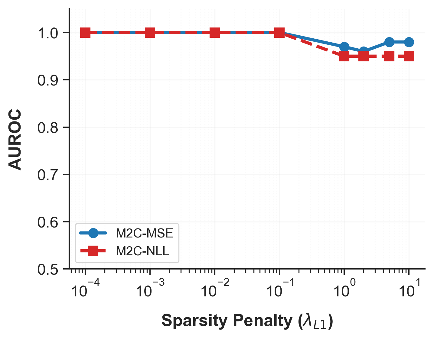


Observations:
-
•
Sparsity Penalty (): As shown in Panel (a), the model is exceptionally robust to the regularization strength, maintaining perfect recovery (AUROC 1.00) for . A slight degradation () is observed only when , where the penalty begins to over-prune weak but true causal signals.
-
•
Sequence Length (): Panel (b) highlights a critical property of the Inverted Variable Embedding. The true lag of the system is small (). Remarkably, even when the input window is extended to , the performance does not degrade (). This confirms that the variable-specific tokenization effectively learns to attend to the relevant immediate history (the first few time steps) while suppressing noise from the distant past, without requiring manual lag selection.
-
•
Latent Dimension (): As seen in Panel (c), the model is insensitive to the hidden dimension size, achieving AUROC for . This suggests that the causal graph structure is the primary information bottleneck, and even compact representations are sufficient to capture the dynamics.
-
•
Diagonal Forcing: Panel (d) demonstrates that our model does not rely on diagonal forcing as a prerequisite for success. Crucially, even in the complete absence of this prior (Force = 0), the model maintains high recovery accuracy (AUROC 0.95 for MSE model, 0.99 for NLL model). This result confirms that diagonal forcing is not a “cheat code” or structural crutch; rather, the model is fully capable of autonomously learning autoregressive dependencies from scratch, with the prior serving merely to accelerate convergence in known autoregressive settings.
Appendix L Forecasting using Causal Pruning
L.1 Model-Specific Pruning Mechanisms
Causal Pruning offers a benefit of reducing architectural complexity from to per node, with implementation strategies specific to each model class. For neural architectures such as MLP and N-BEATS, pruning is enforced by slicing the input tensors so that instead of feeding a full -dimensional vector to the first hidden layer, the model only receives indices corresponding to . In the case of ARIMAX, the set is treated as the collection of exogenous regressors, where masking the exogenous input matrix to include only causal parents allows the model to avoid estimating coefficients for non-causal variables. Similarly, Linear Regression (VAR) is formulated as a sparse Ordinary Least Squares (OLS) problem, ensuring that coefficients are estimated exclusively for variables within the causal neighborhood .
L.2 Comparative Analysis with CUTS+ Baseline
Table 17 compares the performance of different forecasting models for one-step-ahead prediction task by performing causal pruning using causal masks from Mask2Cause and CUTS+ baseline. We observe that for DREAM3 and Lorenz96 datasets, Mask2Cause provides causal matrices that have a better inductive bias. For VAR dataset, we see a slight drop in accuracy which is compensated by lower computational complexity.
| DREAM3 | Lorenz | VAR | ||||||
|---|---|---|---|---|---|---|---|---|
| Model | Ecoli1 | Ecoli2 | Yeast1 | Yeast2 | Yeast3 | F=10 | F=40 | T=500 |
| ARIMAX | +2.25 | +4.16 | +0.67 | +2.57 | +2.74 | +11.40 | -1.92 | -0.38 |
| MLP | +6.31 | +9.70 | +6.31 | +8.02 | +7.93 | +20.66 | +11.70 | -0.52 |
| N-BEATS | +8.19 | +10.79 | +6.36 | +7.82 | +10.34 | +31.24 | +20.59 | -0.62 |
| Linear Reg. | +2.14 | +4.08 | +0.82 | +2.61 | +2.93 | +9.49 | -1.33 | -0.20 |
L.3 Comparison with other Feature Selection Methods
Table 18 provides details of various feature selection mechanisms (Causal Pruning, Mutual Information and Linear Granger Causality) evaluated on parameter reduction and gain in mean square error for common forecasting models. We observe that Causal Pruning, which is a zero-shot byproduct of the Mask2Cause framework, demonstrates competitive results against alternative feature selection methods.
| VAR | Lorenz () | Lorenz () | ||||||||||
| Model / Method | T=500 | T=1000 | T=250 | T=500 | T=250 | T=500 | ||||||
| PR | MSE-R | PR | MSE-R | PR | MSE-R | PR | MSE-R | PR | MSE-R | PR | MSE-R | |
| MLP | ||||||||||||
| M2C (Ours) | 60.01 | -4.41 | 58.60 | -4.06 | 50.84 | +49.35 | 50.04 | +27.61 | 48.37 | +10.33 | 48.87 | +0.55 |
| Mutual Info. | 54.19 | -1.74 | 59.43 | -3.41 | 0.83 | +4.36 | 1.16 | +1.09 | 33.08 | -3.21 | 46.71 | -16.74 |
| Linear Granger | 20.45 | +0.85 | 9.00 | +0.53 | 26.46 | +27.78 | 18.62 | +22.25 | 59.18 | -9.61 | 51.70 | -10.52 |
| ARIMAX | ||||||||||||
| M2C (Ours) | 72.20 | -5.11 | 70.50 | -5.62 | 61.17 | +2.41 | 60.20 | +2.27 | 58.20 | +1.13 | 58.80 | +1.27 |
| Mutual Info. | 65.20 | -2.88 | 71.50 | -3.85 | 1.00 | -0.24 | 1.40 | -0.91 | 39.80 | +3.01 | 56.20 | +0.37 |
| Linear Granger | 24.60 | +0.45 | 10.83 | +0.30 | 31.83 | +2.42 | 22.40 | -0.33 | 71.20 | +3.18 | 62.20 | +1.02 |
| N-BEATS | ||||||||||||
| M2C (Ours) | 4.8 | +10.72 | 4.7 | +1.13 | 7.9 | +20.67 | 7.9 | +5.18 | 7.6 | -11.26 | 7.6 | -27.67 |
| Mutual Info. | 8.47 | +5.68 | 9.28 | -0.69 | 0.13 | -7.82 | 0.18 | -15.73 | 5.17 | -58.71 | 7.30 | -103.78 |
| Linear Granger | 3.19 | +3.34 | 1.41 | +0.92 | 4.13 | +13.35 | 2.91 | +19.04 | 9.24 | -76.56 | 8.08 | -92.93 |
Appendix M Proofs
M.1 Neural Granger Causality is a Special Case of Directed Information
Theorem Let the system evolve according to a Structural Equation Model with Additive Noise: , where is independent, homoscedastic noise. If is functionally non-causal for (i.e., is invariant to ), then Causally Conditioned Directed Information is exactly zero.
Proof.
The Causally Conditioned Directed Information (DI) from a source to a target is defined as the expected sum of Kullback-Leibler (KL) divergences between the full conditional distribution and the restricted conditional distribution:
| (21) |
Under the Additive Noise Model (ANM) assumption, the randomness in arises solely from the noise term . Consequently, the conditional probability density function is equivalent to the noise density shifted by the deterministic prediction function :
| (22) |
If is functionally non-causal for , then by definition, the function does not depend on the history of . Mathematically, this implies invariance:
| (23) |
Substituting this invariance into the density formulation:
| (24) | ||||
Since the full conditional distribution is identical to the restricted distribution at every time step , the KL divergence term vanishes:
| (25) |
Thus, the Causally Conditioned Directed Information is exactly zero. ∎
Remark (Failure of the Converse in Heteroscedastic Systems). It is crucial to note that the converse does not hold for general dynamical systems. If a variable influences the variance (or higher-order moments) of without affecting its conditional mean, then holds, satisfying the condition for Functional Non-Causality (zero NGC). However, in such a case, the probability distributions would differ in shape (e.g., width), i.e., . The Directed Information, which detects any distributional discrepancy, would correctly be non-zero (). This gap highlights precisely why standard functional methods fail on the Mixed Physics benchmark, while probabilistic objectives succeed.
M.2 Proof of Zero Self-Information under Causal Conditioning
Proposition. For any variable , the Causally Conditioned Directed Information from to itself is exactly zero:
| (26) |
Proof.
Recall the definition of Causally Conditioned Directed Information from a source to a target , conditioned on the set of all other variables :
| (27) |
where denotes the full history of all variables in the system up to time .
To evaluate the self-information flow, we set the source variable to be the target itself, i.e., let . In this case, the exclusion set becomes . The term inside the second probability distribution becomes:
| (28) |
This is simply the full system history .
Substituting this back into the KL divergence term:
| (29) |
Since the Kullback-Leibler divergence between two identical distributions is exactly zero (), every term in the summation vanishes. Therefore:
| (30) |
∎
Appendix N Limitations and Broader Impacts
N.1 Limitations
While Mask2Cause successfully captures both mean and variance-driven causality, the heteroscedastic NLL objective fundamentally assumes the underlying conditional distribution is Gaussian. Because Gaussian NLL penalizes errors quadratically, extreme outliers in heavy-tailed data force the network to artificially inflate the predicted variance, which can wash out the structural gradient (potentially leading to spurious edge detection). If heavy tails are detected in the dataset (e.g., via a high kurtosis statistic), the framework can however be trivially adjusted by swapping the Gaussian likelihood for a Student-t or Laplace distribution NLL. Like all methods grounded in the Granger Causality framework, Mask2Cause relies on the assumption of causal sufficiency. It assumes there are no unobserved latent confounders driving the observed variables. In the presence of hidden confounders, Granger-based methods may infer spurious direct edges. Extending this framework to detect or mitigate hidden confounding remains an important direction for future work. Our architecture assumes the causal graph is fixed. While the temporal dynamics themselves are highly non-stationary (yielding time-varying predictive moments), the underlying structural adjacency matrix is assumed to be static across the evaluated time horizon . Adapting the masking mechanism to handle non-stationary, regime-switching causal structures is a promising avenue for further research.
N.2 Broader Impacts
Causal discovery from time series has profound implications across domains ranging from climate science to financial econometrics. On the positive side, robust causal graphs can improve the interpretability and safety of automated decision-making systems (e.g., medical interventions or traffic grid optimization) by distinguishing true mechanisms from spurious correlations. A potential negative impact arises if the models are applied to sensitive human-centric data without accounting for unobserved confounders, which could lead to flawed causal conclusions and biased policy interventions. To mitigate this, practitioners must validate the discovered graphs against domain expertise before deployment.