跳到论文正文
W Papers独立论文阅读器 arXiv:2605.06176 论文正文 计算阅读时间 · 0%
引用这篇论文根据当前论文元数据生成,正式投稿前建议核对。


License: CC Zero
arXiv:2605.06176v1 [math.OC] 07 May 2026

Stochastic Optimal Control for Jump Diffusion Models with Singular Drifts

Antoine-Marie Bogso Faculty of Sciences, Department of Mathematics, University of Yaounde I, P.O. Box 812, Yaounde, Cameroon antoine.bogso@facsciences-uy1.cm , Edward Fuituh Kameh Department of Mathematics and Computer Science, University of Bamenda, Cameroon fekkameh@gmail.com , Olivier Menoukeu Pamen IFAM, Department of Mathematical Sciences, University of Liverpool, L69 7ZL, United Kingdom menoukeu@liverpool.ac.uk and Felix Shu Department of Mathematics and Computer Science, University of Bamenda, Cameroon shufche@gmail.com
Abstract.

We study a stochastic optimal control problem for jump–diffusion systems whose drift coefficient is piecewise Lipschitz continuous and exhibits threshold-induced discontinuities. Such dynamics naturally arise in applications with intervention policies triggered by safety levels, notably in insurance surplus management with dividend payments and capital injections. These features place the problem outside the scope of classical stochastic maximum principle (SMP) results, which rely on global smoothness assumptions. We establish both necessary and sufficient optimality conditions for this class of control problems. Our approach combines a Sobolev-type representation of the first variation process with smooth approximations and Ekeland’s variational principle. As application, we study an optimal premium adjustment and reserve management policies for an insurance whose surplus is modelled by threshold-based dividend and capital injection policies.

Key words and phrases:
Singular SDE; Sobolev differentiable flow; Ekeland’s variational principle; Itô’s formula; Kunita inequality.
2010 Mathematics Subject Classification:
Primary: 60H10, 60H07, 49J55, 60J55, 60H30, Secondary: 60J55, 93E20 ,60H30
This work was partially supported by a grant from the IMU-CDC and Simons Foundation

1. Introduction

Stochastic optimal control problems are fundamental to the modelling and analysis of systems subject to uncertainty, with applications in finance, engineering, and the natural sciences. The aim is to determine a control process that minimizes (or maximizes) an expected cost functional for a system whose dynamics are governed by stochastic differential equations (SDEs). In the classical setting, the controlled system satisfies

d​Xtα=b​(t,Xtα,αt)​d​t+σ​(t,Xtα,αt)​d​Bt,X0α=x0,dX_{t}^{\alpha}=b(t,X_{t}^{\alpha},\alpha_{t})dt+\sigma(t,X_{t}^{\alpha},\alpha_{t})dB_{t},\qquad X_{0}^{\alpha}=x_{0},

where BtB_{t} is a standard Brownian motion, αt\alpha_{t} is an admissible control, and bb and σ\sigma denote the drift and diffusion coefficients. The objective is to characterize the optimal control α^\hat{\alpha} minimizing

J​(α)=𝔼​[∫0Tf​(t,Xtα,αt)​𝑑t+g​(XTα)].J(\alpha)=\mathbb{E}\big[\int_{0}^{T}f(t,X_{t}^{\alpha},\alpha_{t})dt+g(X_{T}^{\alpha})\big].

The stochastic maximum principle (SMP), first introduced by Kushner [12] and further developed in [3, 4, 8, 23, 31], provides necessary (and sometimes sufficient) conditions for optimality via adjoint processes and variational inequalities, under suitable regularity assumptions and convex control sets. Two main approaches exist for solving such problems: the dynamic programming method, leading to the Hamilton–Jacobi–Bellman (HJB) equation, and the SMP or Pontryagin-type approach. The dynamic programming method, pioneered by Bellman, relies on the Markov property and regularity of the value function, whereas the SMP offers a more flexible framework, especially when jumps or non-smooth coefficients are present.

The classical SMP for diffusion models was first established under strong regularity conditions such as global Lipschitz continuity and boundedness of bb and σ\sigma (see for example [23, 29, 31] and references therein). These results were later extended to jump-diffusion systems (see for [22] and references therein).

However, most existing results rely critically on the smoothness (or global Lipschitz continuity) of the drift b​(t,x,α)b(t,x,\alpha) in xx and α\alpha. This assumption guarantees existence and uniqueness of strong solutions and the differentiability of the state process with respect to control perturbations. In many real-world systems, though, such regularity is too restrictive: dynamics may exhibit discontinuities or abrupt changes, as in hybrid systems, threshold-type financial models, switching diffusions, or controlled processes with regime changes. In these cases, where the drift is only piecewise Lipschitz, classical variational methods fail because the first variation process may not exist in the classical sense. These challenges motivate the development of an SMP under weaker regularity assumptions.

Recent studies have addressed SDEs with discontinuous drifts in the Brownian setting (see, e.g., [10, 15, 16, 18] and references therein). More recently, Przemysław and Szölgyenyi [26, 27] examined jump-diffusion models with piecewise Lipschitz drifts, motivated by applications in electricity, insurance, and financial markets. Building on this line of research, recent works [5, 17, 30] have established necessary and sufficient SMPs for Brownian-driven systems with irregular drift. These approaches typically combine smooth approximations of the control problem, Sobolev-type representations of the first variation process, and Ekeland’s variational principle to ensure convergence of the corresponding adjoint processes.

In this paper, we study a stochastic optimal control problem for jump-diffusion systems whose drift coefficient is piecewise Lipschitz continuous. We establish both necessary and sufficient optimality conditions for such systems. The main analytical difficulty arises from the singularity of the drift, which prevents the direct application of classical standard SMP results. Our approach begins with an explicit Sobolev-type representation of the first variation process, followed by the construction of a sequence of approximating problems with smooth coefficients. Using the fact that the law of the state process admits a density with respect to Lebesgue measure, we apply Ekeland’s variational principle to obtain a sequence of adjoint processes and, by passing to the limit, derive an SMP for the original jump-diffusion control problem.

Another key step in our analysis is a convergence result for nonlinear functionals of approximating state processes. In the Brownian additive-noise setting (see, e.g., [5, 17]), Girsanov’s theorem allows one to reduce to expectations involving a Brownian motion, for which explicit Gaussian density estimates are available. Such a reduction is not available in the present jump-diffusion framework. Instead, we exploit the intrinsic regularity of the state process. More precisely, we prove a time-integrated convergence result for compositions of drift approximations with the state process, relying only on uniform moment bounds and a density estimate of order t−1/2t^{-1/2} (see for e.g. Theorem B.2). This estimate plays a central role in passing to the limit in the adjoint equations (see Lemma 3.5) and provides a robust alternative to Girsanov-based arguments under low regularity of the drift.

The main contribution of this paper is the relaxation of the global Lipschitz assumption on the drift to piecewise Lipschitz continuity while retaining a valid stochastic maximum principle for jump-diffusion control systems. This extension broadens the applicability of stochastic control theory to models featuring structural breaks and regime-dependent dynamics.

Threshold-based control policies in insurance and finance often lead to stochastic dynamics with discontinuous yet piecewise Lipschitz drift coefficients. The jump-diffusion surplus model presented in Section 2 provides a concrete illustration of this phenomenon. Such models fall outside the reach of classical stochastic maximum principle results, motivating the theoretical framework developed in this paper.

The remainder of the paper is organised as follows. Section 2 introduces a motivating example and formulates the general control problem. It also presents regularity results for the jump-diffusion SDE with piecewise Lipschitz drift. Both necessary and sufficient conditions for optimality are established in Section 3. Finally, Section 4 applies the theoretical results to an insurance model, analysing the optimal premium adjustment and reserve management policies for an insurer operating under jump risk.

2. A motivating example and preliminary results

2.1. Motivating example and problem formulation

Insurance companies routinely manage large portfolios of liabilities whose values fluctuate due to random claim arrivals and payments. Managing the surplus (the difference between assets and liabilities) requires balancing premium income, capital reserves, and regulatory constraints. This setting naturally leads to a stochastic control problem where the insurer seeks an optimal premium adjustment or reserve policy to maintain financial stability while minimizing risk exposure.

2.1.1. Motivating example

We consider an insurance company whose liability process (or payment function) at time tt is denoted by LtL_{t}, representing the total amount of insurance claims minus the premiums received over the interval [0,t][0,t]. We model the liability using a classical compound Poisson risk model, possibly perturbed by diffusion or jump-diffusion terms. Specifically, the liability of the company at time tt is described by the following SDE:

−d​Lt=(bt+αt)​d​t+σt​d​Bt+d​(∑k=1NtZk),t≥0,L0=l,-\mathrm{d}L_{t}=(b_{t}+\alpha_{t})\,\mathrm{d}t+\sigma_{t}\,\mathrm{d}B_{t}+\mathrm{d}\big(\sum_{k=1}^{N_{t}}Z_{k}\big),\quad t\geq 0,\quad L_{0}=l, (2.1)

where bt≥0b_{t}\geq 0 is the liability rate representing the expected liability (or gain) per unit time due to premium loading, αt\alpha_{t} is the premium rate (or premium policy) which acts as the control variable, and σt>0\sigma_{t}>0 is the volatility measuring liability risk. We assume that the insurer is not allowed to invest in risky assets due to regulatory restrictions.

At the initial time t=0t=0, the insurer deposits an amount X0X_{0} to cover potential future claims exceeding premiums. Let XtX_{t} denote the insurer’s cash balance at time tt, which is composed of the initial capital minus net outflows up to time tt, all accumulated at the compound interest rate. This can be written as

Xt=eΔt​(X0−∫0te−Δ​(s)​dLs),X0=x,X_{t}=e^{\Delta_{t}}\big(X_{0}-\int_{0}^{t}e^{-\Delta(s)}\,\mathrm{d}L_{s}\big),\qquad X_{0}=x, (2.2)

where Δt=∫0tδs​ds\Delta_{t}=\int_{0}^{t}\delta_{s}\,\mathrm{d}s and x≥0x\geq 0 represents the initial reserve. Applying Itô’s formula, the cash balance XtX_{t} satisfies the following SDE:

−d​Xt=(δt​Xt+bt+αt)​d​t+σt​d​Bt+d​(∑k=1NtZk),t∈[0,T],X0=x,-\mathrm{d}X_{t}=(\delta_{t}X_{t}+b_{t}+\alpha_{t})\,\mathrm{d}t+\sigma_{t}\,\mathrm{d}B_{t}+\mathrm{d}\big(\sum_{k=1}^{N_{t}}Z_{k}\big),\qquad t\in[0,T],\quad X_{0}=x, (2.3)

where αt\alpha_{t} is the control variable. Further, assume that when the surplus exceeds a positive threshold HH, the insurer may withdraw a fixed amount (dividend or fee), and when the surplus falls below −H-H, the insurer injects a fixed amount (or reduces net outflows). Incorporating this mechanism, the SDE (2.3) becomes:

{−d​Xt=(δt​Xt+bt+αt−β​sgn​(Xt)​𝟏{|Xt|>H})​d​t+σt​d​Bt+d​(∑k=1NtZk),t∈[0,T],X0=x,\displaystyle\begin{cases}-\mathrm{d}X_{t}=\big(\delta_{t}X_{t}+b_{t}+\alpha_{t}-\beta\,\mathrm{sgn}(X_{t})\mathbf{1}_{\{|X_{t}|>H\}}\big)\,\mathrm{d}t+\sigma_{t}\,\mathrm{d}B_{t}+\mathrm{d}\big(\sum_{k=1}^{N_{t}}Z_{k}\big),\quad t\in[0,T],\\ \quad X_{0}=x,\end{cases}

where β>0\beta>0 represents the magnitude of the fixed drain or injection. The above model maintains the surplus within a target corridor, preventing large oscillations, while also accounting for emergency capital infusion or premium adjustments to avoid ruin. The above equation can be rewritten as:

d​Xtα=\displaystyle\mathrm{d}X^{\alpha}_{t}= −{δt​Xtα+bt+αt−β​sgn​(Xtα)​𝟏{|Xtα|>H}}​d​t−σt​d​Bt−∫ℝ\{0}z​N​(d​z,d​t).\displaystyle-\big\{\delta_{t}X^{\alpha}_{t}+b_{t}+\alpha_{t}-\beta\,\mathrm{sgn}(X^{\alpha}_{t})\mathbf{1}_{\{|X^{\alpha}_{t}|>H\}}\big\}\mathrm{d}t-\sigma_{t}\mathrm{d}B_{t}-\int_{\mathbb{R}\backslash\{0\}}zN(\mathrm{d}z,\mathrm{d}t). (2.4)

We assume that the fund manager’s objective is to determine the optimal rate α\alpha that minimises the second moment of the fund value. In other words, the goal is to find α\alpha that keeps XX as close as possible to zero. More formally, the aim is to identify α^∈𝒜\hat{\alpha}\in\mathcal{A} such that

𝔼​[(XTα^)2]=infα∈𝒜𝔼​[(XTα)2],\mathbb{E}\big[\big(X^{\hat{\alpha}}_{T}\big)^{2}\big]=\inf_{\alpha\in\mathcal{A}}\mathbb{E}\big[(X^{\alpha}_{T})^{2}\big], (2.5)

where α^\hat{\alpha} is an optimal control (if it exists).

Although the drift term in equation (2.4) is discontinuous at HH, it can still be seen as a piecewise Lipschitz function. However, the problem of optimal control for jump-diffusion with piecewise Lipschitz coefficients lies outside the scope of existing literature on stochastic optimal control.

2.1.2. General Problem Formulation

Motivated by the above example, we consider the general controlled jump–diffusion system

Xtα=x+∫0tb​(Xuα,αu)​du+σ​Bt+∫ℝ\{0}γ​(z)​N​(d​z,t),X^{\alpha}_{t}=x+\int_{0}^{t}b(X^{\alpha}_{u},\alpha_{u})\mathrm{d}u+\sigma B_{t}+\int_{\mathbb{R}\backslash\{0\}}\gamma(z)N(\mathrm{d}z,t), (2.6)

where bb is a deterministic function and σ\sigma is a constant vector, BB and NN are dd-dimensional Brownian motion and Poisson random measure on a probability space (Ω,ℱ,P)(\Omega,{\mathcal{F}},P) equipped with the completed filtration (ℱt)t∈[0,T]({\mathcal{F}}_{t})_{t\in[0,T]}. The control variable α:[0,T]×Ω↦𝔸⊂ℝ\alpha:[0,T]\times\Omega\mapsto\mathbb{A}\subset\mathbb{R} is ℬ​([0,T])⊗ℱ\mathcal{B}([0,T])\otimes\mathcal{F}-measurable, and (ℱt)t∈[0,T]({\mathcal{F}}_{t})_{t\in[0,T]}-adapted. 𝔸⊆ℝ\mathbb{A}\subseteq\mathbb{R} is a closed convex subset of ℝ\mathbb{R}

The criterion to be optimised over the set of admissible controls 𝒜\mathcal{A} (see Definition 2.2) has by the following form.

J​(α):=𝔼​[∫0Tf​(s,Xsα,αs)​ds+g​(XTα)],\displaystyle J(\alpha):=\mathbb{E}\big[\int_{0}^{T}f(s,X^{\alpha}_{s},\alpha_{s})\,\mathrm{d}s+g(X^{\alpha}_{T})\big], (2.7)

where ff and gg are function satisfying some conditions. The optimal control problem is the following

Problem 2.1.

Find α^∈Å\hat{\alpha}\in\AA such that

J​(α^)=supα∈𝒜J​(α),\displaystyle J(\hat{\alpha})=\sup_{\alpha\in\mathcal{A}}J(\alpha), (2.8)

.

Definition 2.2.

The set of admissible controls given in Problem 2.1 is defined as:

𝒜:={α:[0,T]×Ω→𝔸, progressive, (2.6) has a unique strong solution and 𝔼supt∈[0,T]|α(t)|4<M for some M>0}.\mathcal{A}:=\big\{\alpha:[0,T]\times\Omega\to\mathbb{A},\text{ progressive, \eqref{eqconpb1}}\text{ has a unique strong solution and }\\ \mathbb{E}\sup_{t\in[0,T]}|\alpha(t)|^{4}<M\text{ for some }M>0\big\}.

The following definition corresponds to [14, Definition 2.1].

Definition 2.3 (piecewise Lipschitz function).

Let I⊂ℝI\subset\mathbb{R} be an interval. A function f:I→ℝf:I\to\mathbb{R} is said to be piecewise Lipschitz if there exist finitely many points ξ1<⋯<ξm∈I\xi_{1}<\cdots<\xi_{m}\in I such that ff is Lipschitz continuous on each of the intervals (−∞,ξ1)∩I,(ξm,∞)∩I(-\infty,\xi_{1})\cap I,\,\,(\xi_{m},\infty)\cap I and (ξk,ξk+1),k=1,…,m−1.(\xi_{k},\xi_{k+1}),\quad k=1,\dots,m-1.

We assume the following conditions on b,fb,f and gg.

Assumption 2.4.
b​(x,a)=b1​(x,a)+b2​(x)+b3​(x),b(x,a)=b_{1}(x,a)+b_{2}(x)+b_{3}(x),

where

  • •

    b1b_{1} is globally bounded and 𝒞1\mathcal{C}^{1} in its first and second variables, with uniformly bounded derivatives

  • •

    b2b_{2} is uniformly bounded and piecewise Lipschitz with k∈ℕk\in\mathbb{N} discontinuities in the points ξ1,…,ξk∈ℝ\xi_{1},\ldots,\xi_{k}\in\mathbb{R}

  • •

    b3b_{3} is 𝒞1\mathcal{C}^{1} with bounded derivative and satisfies a linear growth condition.

  • •

    ff and gg are continuously differentiable in their arguments;

  • •

    there exists C>0C>0 such that

    |f​(t,x,a)|+|∂xf​(t,x,a)|+|∂af​(t,x,a)|≤C​(1+|x|2+|a|2),for all ​(t,x,a)|f(t,x,a)|+|\partial_{x}f(t,x,a)|+|\partial_{a}f(t,x,a)|\leq C(1+|x|^{2}+|a|^{2}),\quad\text{for all }(t,x,a)

    and

    |g​(x)|+|∂xg​(x)|≤C​(1+|x|2).|g(x)|+|\partial_{x}g(x)|\leq C(1+|x|^{2}).

Note that the controlled SDE in the motivating example,

d​Xtα=(δt​Xtα+bt+αt−β​sgn​(Xtα)​𝟏{|Xtα|>H})​d​t+σt​d​Bt+∫ℝ∖{0}z​N~​(d​z,d​t),\mathrm{d}X_{t}^{\alpha}=\big(\delta_{t}X_{t}^{\alpha}+b_{t}+\alpha_{t}-\beta\,\mathrm{sgn}(X_{t}^{\alpha})\mathbf{1}_{\{|X_{t}^{\alpha}|>H\}}\big)\mathrm{d}t+\sigma_{t}\,\mathrm{d}B_{t}+\int_{\mathbb{R}\setminus\{0\}}z\,\tilde{N}(\mathrm{d}z,\mathrm{d}t), (2.9)

is a particular case of (2.6). In the subsequent section, we provide results on existence, uniqueness, and regularity for the state equation (2.6), laying the foundation for establishing Pontryagin-type necessary and sufficient conditions under piecewise Lipschitz drift coefficients.

The main novelty of this work lies in the analysis of stochastic optimal control problems driven by jump–diffusion dynamics with piecewise Lipschitz drift coefficients. Such drift structures naturally arise in practical financial and insurance models involving threshold-type mechanisms, such as dividend distribution, capital injection, or premium adjustment rules. We develop new sufficient and necessary Pontryagin-type maximum principles under these weaker regularity assumptions, thereby extending the applicability of stochastic control theory to a broader class of discontinuous financial systems.

2.2. Regularity of SDE with piecewise Lipschitz coefficient with jumps

In this section, we consider the SDE

Xtx=x+∫0tb​(Xux)​du+σ​Bt+∫0t∫ℝ\{0}γ​(z)​N​(d​z,d​t),X^{x}_{t}=x+\int_{0}^{t}b(X^{x}_{u})\mathrm{d}u+\sigma B_{t}+\int_{0}^{t}\int_{\mathbb{R}\backslash\{0\}}\gamma(z)N(\mathrm{d}z,\mathrm{d}t), (2.10)

where bb is piecewise Lipschitz with k∈ℕk\in\mathbb{N} discontinuities in the points ξ1,…,ξk∈ℝ\xi_{1},\ldots,\xi_{k}\in\mathbb{R} and bb also satisfies linear growth condition. More precisely bb satisfies

Assumption 2.5.
b=b1+b2,b=b_{1}+b_{2},

where

  • •

    b1b_{1} is Lipschitz and satisfies a linear growth condition;

  • •

    b2b_{2} is uniformly bounded and piecewise Lipschitz with k∈ℕk\in\mathbb{N} discontinuities in the points ξ1,…,ξk∈ℝ\xi_{1},\ldots,\xi_{k}\in\mathbb{R}

It is well known from [27, Theorem 4.1] that the SDE (2.10) has a unique strong solution. In this section we want to show that the solution is Sobolev differentiable with respect to its initial condition and the derivative has an explicit representation.

To do that, let (Xtx,n)n∈ℕ(X^{x,n}_{t})_{n\in\mathbb{N}} be a sequence of strong solutions to the approximating equations (2.10), where the drift coefficients bn=b1+b2,nb_{n}=b_{1}+b_{2,n} replace b=b1+b2b=b_{1}+b_{2}, respectively. More precisely, for each n≥1n\geq 1, define

bn:=b1+b2,n,b_{n}:=b_{1}+b_{2,n},

where {b2,n}n≥1\{b_{2,n}\}_{n\geq 1} are sequences of smooth functions with compact support such that {b2,n}n≥1\{b_{2,n}\}_{n\geq 1} is piecewise Lipschitz and

b2,n​(x)→b2​(x),(x)​-a.e. as ​n→∞,and ​supn≥1‖b2,n‖∞<∞.b_{2,n}(x)\to b_{2}(x),\quad(x)\text{-a.e. as }n\to\infty,\quad\text{and }\sup_{n\geq 1}\|b_{2,n}\|_{\infty}<\infty.

The existence and uniqueness of Xtn,xX^{n,x}_{t} follows from classical results on SDEs with jumps (see [1, 11]). In addition, Xtn,xX^{n,x}_{t} is Malliavin differentiable and admits a first variation process whose equation is given by (see for example [11, Theorem 3.3.2]):

∂Xtn,x∂x=1+∫0tbn′​(Xun,x)​∂Xun,x∂x​du=exp⁡{∫0tbn′​(Xun,x)​du},\frac{\partial X^{n,x}_{t}}{\partial x}=1+\int_{0}^{t}b^{\prime}_{n}(X^{n,x}_{u})\frac{\partial X^{n,x}_{u}}{\partial x}\mathrm{d}u=\exp\big\{\int_{0}^{t}b^{\prime}_{n}(X^{n,x}_{u})\mathrm{d}u\big\}, (2.11)

where bn′b^{\prime}_{n} denotes the derivative of bnb_{n}. In the next Lemma, we show that the sequence (Xtn,x)n∈ℕ(X^{n,x}_{t})_{n\in\mathbb{N}} converges strongly in L2​(Ω,ℱ,ℙ)L^{2}(\Omega,\mathcal{F},\mathbb{P}).

Lemma 2.6.

Let bb be as in Assumption 2.5 and let (bn)n≥1(b_{n})_{n\geq 1} given as above. Let X⋅n,xX^{n,x}_{\cdot} denote the strong solution of the SDE driven by the vector field bnb_{n}, and let X⋅xX^{x}_{\cdot} be a strong solution of the SDE associated with bb. Then, the sequence {Xtn,x}n≥1\{X^{n,x}_{t}\}_{n\geq 1} satisfies

Xtn,x→Xtxstrongly in ​L2​(Ω,ℙ)as ​n→∞.X^{n,x}_{t}\rightarrow X^{x}_{t}\quad\text{strongly in }L^{2}(\Omega,\mathbb{P})\quad\text{as }n\to\infty.
Proof.

See Appendix A ∎

From now on we assume the following:

Theorem 2.7.

Under Assumption 2.5, the first variation process (in the Sobolev sense) of the strong solution XtxX^{x}_{t}, to the SDE (2.10) exists and has the following explicit representation

∂Xtx∂x=\displaystyle\frac{\partial X^{x}_{t}}{\partial x}= exp{∫0tb1′(Xux)du+2(b~2(Xtx)−b~2(x)−∫0tb1(Xux)b2(Xux)du\displaystyle\exp\big\{\int_{0}^{t}b_{1}^{\prime}(X^{x}_{u})\mathrm{d}u+2\big(\tilde{b}_{2}(X^{x}_{t})-\tilde{b}_{2}(x)-\int_{0}^{t}b_{1}(X^{x}_{u})b_{2}(X^{x}_{u})\mathrm{d}u
−∫0tb22​(Xux)​du−∫0tb2​(Xux)​dBu\displaystyle-\int_{0}^{t}b_{2}^{2}(X^{x}_{u})\mathrm{d}u-\int_{0}^{t}b_{2}(X^{x}_{u})\mathrm{d}B_{u}
−∫0t∫ℝ\{0}{b~2(Xux+γ(z))−b~2(Xux)}N(dz,du))},\displaystyle-\int_{0}^{t}\int_{\mathbb{R}\backslash\{0\}}\big\{\tilde{b}_{2}(X^{x}_{u}+\gamma(z))-\tilde{b}_{2}(X^{x}_{u})\big\}N(\mathrm{d}z,\mathrm{d}u)\big)\big\}, (2.12)

where b~2​(x)=∫−∞xb2​(y)​dy.\tilde{b}_{2}(x)=\int_{-\infty}^{x}b_{2}(y)\mathrm{d}y. In addition there exists a constant C>0C>0 depending on the Lipschitz constant of b1b_{1}, ‖b2‖∞,T,p\|b_{2}\|_{\infty},T,p, such that

𝔼​[|∂Xtx∂x|p]≤C.\displaystyle\mathbb{E}\big[\big|\frac{\partial X^{x}_{t}}{\partial x}\big|^{p}\big]\leq C. (2.13)
Proof.

See Appendix A.

∎

3. Stochastic Maximum Principle

3.1. Main results

The main results of this work are the following necessary and sufficient conditions in the Pontryagin stochastic maximum principle.

Theorem 3.1.

Suppose that bb satisfies Assumption 2.4. Let α^∈𝒜\hat{\alpha}\in\mathcal{A} be an optimal control and let Xα^X^{\hat{\alpha}} be the associated optimal trajectory. Then the first variation process Φα^\Phi^{\hat{\alpha}} of Xα^X^{\hat{\alpha}} is well-defined and it holds

∂aH​(t,Xtα^,Ptα^,α^t)⋅(β−α^t)≥0ℙ⊗d​t​-a.s. for all ​β∈𝒜,\partial_{a}H(t,X^{\hat{\alpha}}_{t},P^{\hat{\alpha}}_{t},\hat{\alpha}_{t})\cdot(\beta-\hat{\alpha}_{t})\geq 0\quad\mathbb{P}\otimes\,\mathrm{d}t\text{-a.s. for all }\beta\in\mathcal{A}, (3.1)

where Pα^P^{\hat{\alpha}} is the adjoint process given by

Ptα^:=𝔼​[Φt,Tα^​∂xg​(XTα^)+∫tTΦt,sα^​∂xf​(s,Xsα^,α^s)​d​s∣ℱt],P^{\hat{\alpha}}_{t}:=\mathbb{E}\Big[\Phi^{\hat{\alpha}}_{t,T}\partial_{x}g(X^{\hat{\alpha}}_{T})+\int_{t}^{T}\Phi^{\hat{\alpha}}_{t,s}\partial_{x}f(s,X^{\hat{\alpha}}_{s},\hat{\alpha}_{s})\mathrm{d}s\mid\mathcal{F}_{t}\Big], (3.2)

with Φα\Phi^{\alpha} given by

Φt,sα=\displaystyle\Phi^{\alpha}_{t,s}= exp{∫ts∂xb1(Xuα,x,αu)du+∫ts∂xb3(Xuα,x)du\displaystyle\exp\big\{\int_{t}^{s}\partial_{x}b_{1}(X^{\alpha,x}_{u},\alpha_{u})\mathrm{d}u+\int_{t}^{s}\partial_{x}b_{3}(X^{\alpha,x}_{u})\mathrm{d}u
+2(b~2(Xsα,x)−b~2(Xtα,x)−∫ssb22(Xuα,x)du−∫0tb2(Xuα,x)dBu\displaystyle+2\big(\tilde{b}_{2}(X^{\alpha,x}_{s})-\tilde{b}_{2}(X^{\alpha,x}_{t})-\int_{s}^{s}b_{2}^{2}(X^{\alpha,x}_{u})\mathrm{d}u-\int_{0}^{t}b_{2}(X^{\alpha,x}_{u})\mathrm{d}B_{u}
−∫tsb1​(Xuα,x,αu)​b2​(Xuα,x)​du\displaystyle-\int_{t}^{s}b_{1}(X^{\alpha,x}_{u},\alpha_{u})b_{2}(X^{\alpha,x}_{u})\mathrm{d}u
−∫ts∫ℝ\{0}{b~2(Xuα,x+γ(z))−b~2(Xuα,x)}N(dz,du))},\displaystyle-\int_{t}^{s}\int_{\mathbb{R}\backslash\{0\}}\big\{\tilde{b}_{2}(X^{\alpha,x}_{u}+\gamma(z))-\tilde{b}_{2}(X^{\alpha,x}_{u})\big\}N(\mathrm{d}z,\mathrm{d}u)\big)\big\},

where b~2​(x)=∫−∞xb2​(y)​dy.\tilde{b}_{2}(x)=\int_{-\infty}^{x}b_{2}(y)\mathrm{d}y.

Proof.

See Section 3.2. ∎

Theorem 3.2.

Let the conditions of Theorem 3.1 be satisfied. Let α∈𝒜\alpha\in\mathcal{A} and let Xα^X^{\hat{\alpha}} be the associated trajectory and Ptα^P^{\hat{\alpha}}_{t} be the corresponding adjoint given by (3.2). In addition, assume that gg and (x,a)↦H​(t,x,Ptα^,a)(x,a)\mapsto H(t,x,P^{\hat{\alpha}}_{t},a) are concave for all t∈[0,T]t\in[0,T]. Further assume that

∂aH​(t,Xtα^,Ptα^,α^t)=0ℙ⊗d​t​-a.s.\partial_{a}H(t,X^{\hat{\alpha}}_{t},P^{\hat{\alpha}}_{t},\hat{\alpha}_{t})=0\quad\mathbb{P}\otimes\,\mathrm{d}t\text{-a.s.} (3.3)

Then, α^\hat{\alpha} is an optimal control.

We denote by dd the distance

d​(α1,α2):=𝔼​[supt∈[0,T]|αt1−αt2|4]1/4.d(\alpha^{1},\alpha^{2}):=\mathbb{E}\big[\sup_{t\in[0,T]}|\alpha_{t}^{1}-\alpha_{t}^{2}|^{4}\big]^{1/4}. (3.4)
Proof.

See Section 3.2. ∎

Proof strategy. The argument proceeds in three steps:

  1. (1)

    Step 1. Using Ekeland’s variational principle, we show that an optimal control for problem (2.6) is also optimal for a suitably perturbed version of the approximating problem with value Vn​(x0)V_{n}(x_{0}).

  2. (2)

    Step 2. For the approximating problem with smooth drift coefficients, we derive a maximum principle involving the state process Xnα^nX_{n}^{\hat{\alpha}^{n}} and its associated first variation process Φnα^n\Phi^{\hat{\alpha}^{n}}_{n}.

  3. (3)

    Step 3. The final and most delicate step consists in passing to the limit as n→∞n\rightarrow\infty and establishing a stability property of the maximum principle.

We begin by addressing this limit step through a series of preparatory lemmas whose proofs are (deferred to the next section), which will be assembled to establish Theorem 3.1 at the end of this section.

Lemma 3.3.

We have the following bounds:

  • (i)

    For every sequence (αn)n(\alpha^{n})_{n} in 𝒜\mathcal{A}, it holds sup𝑛​𝔼​[supt∈[0,T]|Xtn,αn|2]<∞\underset{n}{\sup}\mathbb{E}\big[\sup_{t\in[0,T]}|X^{n,\alpha^{n}}_{t}|^{2}\big]<\infty.

  • (ii)

    For every α1,α2∈𝒜\alpha^{1},\alpha^{2}\in\mathcal{A} it holds

    𝔼​[|Xtn,α1−Xtα2|2]≤C​(d​(α1,α2)4+∫0T∫ℝ|b2,n​(x)−b2​(x)|4​ρsα2​(x)​dx​ds),\mathbb{E}\big[|X^{n,\alpha^{1}}_{t}-X^{\alpha^{2}}_{t}|^{2}\big]\leq C\big(d(\alpha^{1},\alpha^{2})^{4}+\int_{0}^{T}\int_{\mathbb{R}}|b_{2,n}(x)-b_{2}(x)|^{4}\rho^{\alpha^{2}}_{s}(x)\mathrm{d}x\mathrm{d}s\big),

    where ρsα2\rho^{\alpha^{2}}_{s} is the density of Xsα2X^{\alpha^{2}}_{s}

  • (iii)

    Given k∈ℕk\in\mathbb{N}, for every sequence (αn)n≥1(\alpha^{n})_{n\geq 1} in 𝒜\mathcal{A} and α∈𝒜\alpha\in\mathcal{A} such that δ​(αn,α)→0\delta(\alpha^{n},\alpha)\rightarrow 0, it holds that

    𝔼​[|Xtk,αn−Xtk,α|2]→0​ as ​n→∞.\mathbb{E}\big[|X^{k,\alpha^{n}}_{t}-X^{k,\alpha}_{t}|^{2}\big]\to 0\text{ as }n\rightarrow\infty.
Proof.

See Section 3.2. ∎

Lemma 3.4.

Let α∈𝒜\alpha\in\mathcal{A} and let αn\alpha^{n} be a sequence of admissible controls satisfying d​(αn,α)→0d(\alpha^{n},\alpha)\to 0. Then, we have

  • (i)

    |Jk​(αn)−Jk​(α)|→0|J_{k}(\alpha^{n})-J_{k}(\alpha)|\to 0 as n→∞n\to\infty for every k∈ℕk\in\mathbb{N} fixed. In other words, the function Jk:(𝒜,d)→ℝJ_{k}:(\mathcal{A},d)\to\mathbb{R} is continuous for each fix k∈ℕk\in\mathbb{N}.

  • (ii)

    There exists a constant C>0C>0 such that |Jn​(α)−J​(α)|≤C​εn|J_{n}(\alpha)-J(\alpha)|\leq C\varepsilon_{n}, with εn↓0\varepsilon_{n}\downarrow 0.

Proof.

See Section 3.2. ∎

Let us now state the stability result for both the first variation and of the adjoint processes.

Lemma 3.5.

Let α∈𝒜\alpha\in\mathcal{A} and αn\alpha^{n} be a sequence of admissible controls such that d​(αn,α)→0d(\alpha^{n},\alpha)\to 0. Then, the processes XnαnX^{\alpha^{n}}_{n} and XαX^{\alpha} admit Sobolev differentiable flows denoted Φnαn\Phi^{\alpha^{n}}_{n} and Φα\Phi^{\alpha}, respectively and for every 0≤t≤s≤T0\leq t\leq s\leq T we have

  • (i)

    𝔼​[|Φt,sn,αn−Φt,sα|2]→0\mathbb{E}\big[|\Phi^{n,\alpha^{n}}_{t,s}-\Phi^{\alpha}_{t,s}|^{2}\big]\to 0 as n→∞n\to\infty,

  • (ii)

    𝔼​[|Ptn,αn−Ptα|]→0\mathbb{E}\big[|P^{n,\alpha^{n}}_{t}-P^{\alpha}_{t}|\big]\to 0 as n→∞n\to\infty,

where PαP^{\alpha} is the adjoint process defined as

Ptα:=𝔼​[Φt,Tα​∂xg​(XTα)+∫tTΦt,sα​∂xf​(s,Xsα,αs)​d​s∣ℱt],P^{\alpha}_{t}:=\mathbb{E}\Big[\Phi^{\alpha}_{t,T}\partial_{x}g(X^{\alpha}_{T})+\int_{t}^{T}\Phi^{\alpha}_{t,s}\partial_{x}f(s,X^{\alpha}_{s},\alpha_{s})\mathrm{d}s\mid\mathcal{F}_{t}\Big],

and PnαnP^{\alpha^{n}}_{n} is defined similarly, with (Xα,α,Φα)(X^{\alpha},\alpha,\Phi^{\alpha}) replaced by (Xn,αn,αn,Φn,αn)(X^{n,\alpha^{n}},\alpha^{n},\Phi^{n,\alpha^{n}}).

Proof.

See Section 3.2. ∎

3.2. Proof of the Main results

Proof of Theorem 3.1.

Let α^\hat{\alpha} be an optimal control and fix n≥1n\geq 1. Under the linear growth assumptions on ff and gg, the functional JnJ_{n} is bounded from above. By Lemma 3.4, JnJ_{n} is continuous on (𝒜,d)(\mathcal{A},d) and there exists εn\varepsilon_{n} such that

J​(α^)−Jn​(α^)≤εn​ and ​Jn​(α)−J​(α)≤εnfor all ​α∈𝒜.J(\hat{\alpha})-J_{n}(\hat{\alpha})\leq\varepsilon_{n}\text{ and }J_{n}(\alpha)-J(\alpha)\leq\varepsilon_{n}\quad\text{for all }\alpha\in\mathcal{A}.

Hence, Jn​(α^)≤infα∈𝒜Jn​(α)+2​εnJ_{n}(\hat{\alpha})\leq\inf_{\alpha\in\mathcal{A}}J_{n}(\alpha)+2\varepsilon_{n}. Therefore, by the Ekeland’s variational principle (see [6]), there exists a control α^n∈𝒜\hat{\alpha}^{n}\in\mathcal{A} such that d​(α^,α^n)≤(2​εn)1/2d(\hat{\alpha},\hat{\alpha}^{n})\leq(2\varepsilon_{n})^{1/2} and

Jn​(α^n)≤Jn​(α)+(2​εn)1/2​d​(α^n,α)for allα∈𝒜.J_{n}(\hat{\alpha}^{n})\leq J_{n}(\alpha)+(2\varepsilon_{n})^{1/2}d(\hat{\alpha}^{n},\alpha)\quad\text{for all}\quad\alpha\in\mathcal{A}.

Define the perturbed functional

Jnεn​(α):=Jn​(α)+(2​εn)1/2​d​(α^n,α),J^{\varepsilon_{n}}_{n}(\alpha):=J_{n}(\alpha)+(2\varepsilon_{n})^{1/2}d(\hat{\alpha}^{n},\alpha),

so that the control α^n\hat{\alpha}^{n} is optimal for the problem with performance functional JnεnJ^{\varepsilon_{n}}_{n}.

Let β∈𝒜\beta\in\mathcal{A} be an arbitrary and fix ε>0\varepsilon>0. Set η=ηn:=β−α^n\eta=\eta_{n}:=\beta-\hat{\alpha}^{n}. By the convexity of 𝔸\mathbb{A}, we have α^n+ε​η∈𝒜\hat{\alpha}^{n}+\varepsilon\eta\in\mathcal{A}. Thanks to the smoothness of bnb_{n}, the functional JnJ_{n} is Gâteau differentiable, with derivative in the direction η\eta given by

dd​ε​Jn​(α^n+ε​η)|ε=0\displaystyle\frac{\mathrm{d}}{\mathrm{d}\varepsilon}J_{n}(\hat{\alpha}^{n}+\varepsilon\eta)_{|_{\varepsilon=0}} =𝔼[∫0T∂xf(t,Xtn,α^n,α^tn)Vtn+∂αf(t,Xtn,α^n,α^tn)ηtdt\displaystyle=\mathbb{E}\big[\int_{0}^{T}\partial_{x}f(t,X^{n,\hat{\alpha}^{n}}_{t},\hat{\alpha}^{n}_{t})V^{n}_{t}+\partial_{\alpha}f(t,X^{n,\hat{\alpha}^{n}}_{t},\hat{\alpha}^{n}_{t})\eta_{t}\mathrm{d}t
+∂xg(XTn,α^n)VTn],\displaystyle\qquad+\partial_{x}g(X^{n,\hat{\alpha}^{n}}_{T})V^{n}_{T}\big],

where VnV_{n} solves the corresponding linear equation

d​Vn​(t)=∂xbn​(t,Xtn,α,αt)​Vtn​d​t+∂αbn​(t,Xtn,α,αt)​ηt​d​t,Vn​(0)=0.\mathrm{d}V^{n}(t)=\partial_{x}b_{n}(t,X^{n,\alpha}_{t},\alpha_{t})V^{n}_{t}\mathrm{d}t+\partial_{\alpha}b_{n}(t,X^{n,\alpha}_{t},\alpha_{t})\eta_{t}\mathrm{d}t,\quad V^{n}(0)=0.

Conversely, by the triangle inequality, we obtain

limε↓01ε​(d​(α^n,α+ε​η)−d​(α^n,α))≤ε​𝔼​[supt∈[0,T]|ηt|4]1/4.\lim_{\varepsilon\downarrow 0}\frac{1}{\varepsilon}\big(d(\hat{\alpha}^{n},\alpha+\varepsilon\eta)-d(\hat{\alpha}^{n},\alpha)\big)\leq\varepsilon\mathbb{E}\big[\sup_{t\in[0,T]}|\eta_{t}|^{4}\big]^{1/4}.

Hence, JnεnJ^{\varepsilon_{n}}_{n} is Gâteau differentiable and the optimality of α^n\hat{\alpha}^{n} for JnεnJ^{\varepsilon_{n}}_{n} implies that

0≤dd​ε​Jnεn​(α^n+ε​η)|ε=0=\displaystyle 0\leq\frac{\mathrm{d}}{\mathrm{d}\varepsilon}J^{\varepsilon_{n}}_{n}(\hat{\alpha}^{n}+\varepsilon\eta)_{|_{\varepsilon=0}}= dd​ε​Jn​(α^n+ε​η)|ε=0+limε↓0(2​εn)1/2​1ε​d​(α^n,α^n+ε​η)\displaystyle\frac{\mathrm{d}}{\mathrm{d}\varepsilon}J_{n}(\hat{\alpha}^{n}+\varepsilon\eta)_{|_{\varepsilon=0}}+\lim_{\varepsilon\downarrow 0}(2\varepsilon_{n})^{1/2}\frac{1}{\varepsilon}d(\hat{\alpha}^{n},\hat{\alpha}^{n}+\varepsilon\eta)
≤\displaystyle\leq 𝔼[∫0T∂xf(t,Xtn,α^n,α^tn)Vtn+∂αf(t,Xtn,α^n,α^tn)ηtdt\displaystyle\mathbb{E}\big[\int_{0}^{T}\partial_{x}f\big(t,X^{n,\hat{\alpha}^{n}}_{t},\hat{\alpha}^{n}_{t}\big)V^{n}_{t}+\partial_{\alpha}f\big(t,X^{n,\hat{\alpha}^{n}}_{t},\hat{\alpha}^{n}_{t}\big)\eta_{t}\mathrm{d}t
+∂xg(XTn,α^n)VTn]+(2εn)1/2(E[supt|ηt|4])1/4\displaystyle+\partial_{x}g(X^{n,\hat{\alpha}^{n}}_{T})V^{n}_{T}\big]+\big(2\varepsilon_{n})^{1/2}(E[\sup_{t}|\eta_{t}|^{4}]\big)^{1/4}
≤\displaystyle\leq 𝔼​[∫0T∂αHn​(t,Xtn,α^,Ptn,α^n,α^tn)​ηt​d​t]+CM​εn1/2,\displaystyle\mathbb{E}\big[\int_{0}^{T}\partial_{\alpha}H_{n}\big(t,X^{n,\hat{\alpha}}_{t},P^{n,\hat{\alpha}^{n}}_{t},\hat{\alpha}^{n}_{t}\big)\eta_{t}\mathrm{d}t\big]+C_{M}\varepsilon_{n}^{1/2},

for a constant CM>0C_{M}>0 depending on the constant MM (as introduced in the definition of 𝒜\mathcal{A}). The inequality follows since α^n∈𝒜\hat{\alpha}^{n}\in\mathcal{A}, and HnH_{n} denotes the Hamiltonian of the problem corresponding to the drift bnb_{n} given by

Hn​(t,x,p,a):=f​(t,x,a)+{bn​(t,x,a)+∫ℝ0γ​(z)​ν​(d​z)}​pH_{n}(t,x,p,a):=f(t,x,a)+\{b_{n}(t,x,a)+\int_{\mathbb{R}_{0}}\gamma(z)\nu(\mathrm{d}z)\}p

and (Pn,α^n,Zn,α^n,Rn,α^n​(z))(P^{n,\hat{\alpha}^{n}},Z^{n,\hat{\alpha}^{n}},R^{n,\hat{\alpha}^{n}}(z)) the adjoint processes satisfying

d​Ptn,α^n=−∂xHn​(t,Xtn,α^n,Ptn,α^n,α^tn)​d​t+Ztn,α^n​d​Bt+∫ℝ0Rtn,α^n​(z)​N~​(d​z,d​t).\mathrm{d}P^{n,\hat{\alpha}^{n}}_{t}=-\partial_{x}H_{n}(t,X^{n,\hat{\alpha}^{n}}_{t},P^{n,\hat{\alpha}^{n}}_{t},\hat{\alpha}^{n}_{t})\mathrm{d}t+Z^{n,\hat{\alpha}^{n}}_{t}\mathrm{d}B_{t}+\int_{\mathbb{R}_{0}}R_{t}^{n,\hat{\alpha}^{n}}(z)\tilde{N}(\mathrm{d}z,\mathrm{d}t).

By standard arguments, we have

CMεn1/2+∂αHn(t,Xtn,α^n,Ptn,α^n,α^tn)⋅(β−α^tn))≥0ℙ⊗dt−a.s.C_{M}\varepsilon_{n}^{1/2}+\partial_{\alpha}H_{n}(t,X^{n,\hat{\alpha}^{n}}_{t},P^{n,\hat{\alpha}^{n}}_{t},\hat{\alpha}^{n}_{t})\cdot(\beta-\hat{\alpha}^{n}_{t}))\geq 0\quad\mathbb{P}\otimes\mathrm{d}t\mathrm{-a.s}.

Since b2,nb_{2,n} does not depend on α\alpha, this reduces to

CM​εn1/2+{∂αf​(t,Xtn,α^n,α^tn)+∂αb1​(t,Xtn,α^n,α^tn)​Ptn,α^n}⋅(β−α^tn)≥0ℙ⊗d​t​-a.s.C_{M}\varepsilon_{n}^{1/2}+\big\{\partial_{\alpha}f(t,X^{n,\hat{\alpha}^{n}}_{t},\hat{\alpha}^{n}_{t})+\partial_{\alpha}b_{1}\big(t,X^{n,\hat{\alpha}^{n}}_{t},\hat{\alpha}^{n}_{t}\big)P^{n,\hat{\alpha}^{n}}_{t}\big\}\cdot(\beta-\hat{\alpha}^{n}_{t})\geq 0\quad\mathbb{P}\otimes\mathrm{d}t\text{-a.s.}

Taking the limit as n→∞n\rightarrow\infty, Lemmas 3.3 and 3.5 ensure that Xtn,α^n→Xtα^X^{n,\hat{\alpha}^{n}}_{t}\to X_{t}^{\hat{\alpha}} and Ptn,α^n→Ptα^P^{n,\hat{\alpha}^{n}}_{t}\to P^{\hat{\alpha}}_{t} ℙ\mathbb{P}-a.s. for all t∈[0,T]t\in[0,T]. Thus, using α^n→α\hat{\alpha}^{n}\to\alpha, we obtain

{∂αf​(t,Xtα^,α^t)+∂αb1​(t,Xtα^,α^t)​Ptα^}⋅(β−α^t)≥0ℙ⊗d​t​-a.s.\big\{\partial_{\alpha}f(t,X^{\hat{\alpha}}_{t},\hat{\alpha}_{t})+\partial_{\alpha}b_{1}\big(t,X^{\hat{\alpha}}_{t},\hat{\alpha}_{t}\big)P^{\hat{\alpha}}_{t}\big\}\cdot(\beta-\hat{\alpha}_{t})\geq 0\quad\mathbb{P}\otimes\mathrm{d}t\text{-a.s.}

This shows (3.1), which concludes the proof. ∎

Proof of Theorem 3.2.

Let α^∈𝒜\hat{\alpha}\in\mathcal{A} satisfy (3.3) and α′\alpha^{\prime} an arbitrary element of 𝒜\mathcal{A}. We would like to show that J​(α^)≥J​(α′)J(\hat{\alpha})\geq J(\alpha^{\prime}). Let n∈ℕn\in\mathbb{N} be arbitrarily chosen. By definition, we have

Jn​(α^)−Jn​(α′)\displaystyle J_{n}(\hat{\alpha})-J_{n}(\alpha^{\prime})
=𝔼​[g​(XTn,α^)−g​(XTn,α′)+∫0Tf​(u,Xun,α^,α^u)−f​(u,Xun,α′,αu′)​d​u]\displaystyle=\mathbb{E}\big[g(X^{n,\hat{\alpha}}_{T})-g(X^{n,\alpha^{\prime}}_{T})+\int_{0}^{T}f(u,X_{u}^{n,\hat{\alpha}},\hat{\alpha}_{u})-f(u,X_{u}^{n,\alpha^{\prime}},\alpha^{\prime}_{u})\,\mathrm{d}u\big]
≥𝔼[∂xg(XTn,α^){XTα^−XTn,α′}+∫0T{bn(u,Xun,α′,αu′)−bn(u,Xun,α^,α^u)}Pun,α^du\displaystyle\geq\mathbb{E}\big[\partial_{x}g(X^{n,\hat{\alpha}}_{T})\big\{X^{\hat{\alpha}}_{T}-X^{n,\alpha^{\prime}}_{T}\big\}+\int_{0}^{T}\big\{b_{n}(u,X^{n,\alpha^{\prime}}_{u},\alpha^{\prime}_{u})-b_{n}(u,X_{u}^{n,\hat{\alpha}},\hat{\alpha}_{u})\big\}P^{n,\hat{\alpha}}_{u}\,\mathrm{d}u
+∫0THn(u,Xun,α^,Pun,α^,α^u)−Hn(u,Xun,α′,Pun,α^,αu′)du],\displaystyle\quad+\int_{0}^{T}H_{n}(u,X_{u}^{n,\hat{\alpha}},P_{u}^{n,\hat{\alpha}},\hat{\alpha}_{u})-H_{n}(u,X_{u}^{n,\alpha^{\prime}},P_{u}^{n,\hat{\alpha}},\alpha^{\prime}_{u})\,\mathrm{d}u\big],

where we used the definition of HnH_{n} and the fact that gg is concave. Since Pnα^P_{n}^{\hat{\alpha}} satisfies

Ptn,α^=𝔼​[Φt,Tn,α^​∂xg​(XTn,α^)+∫tTΦt,un,α^​∂xf​(u,Xun,α^,α^u)​d​u∣ℱt],P^{n,\hat{\alpha}}_{t}=\mathbb{E}\big[\Phi_{t,T}^{n,\hat{\alpha}}\partial_{x}g(X^{n,\hat{\alpha}}_{T})+\int_{t}^{T}\Phi_{t,u}^{n,\hat{\alpha}}\partial_{x}f(u,X_{u}^{n,\hat{\alpha}},\hat{\alpha}_{u})\mathrm{d}u\mid\mathcal{F}_{t}\big],

it follows by the martingale representation and the Itô’s formula that there is a square integrable progressive process (Pnα^,Znα^,Run,α^)(P^{\hat{\alpha}}_{n},Z^{\hat{\alpha}}_{n},R_{u}^{n,\hat{\alpha}}) such that Pnα^P_{n}^{\hat{\alpha}} satisfies the equation

Ptn,α^=\displaystyle P^{n,\hat{\alpha}}_{t}= ∂xg​(XTn,α^)+∫tT∂xHn​(u,Xun,α^,Pun,α^,α^u)​d​u−∫tTZun,α^​dWu\displaystyle\partial_{x}g(X^{n,\hat{\alpha}}_{T})+\int_{t}^{T}\partial_{x}H_{n}(u,X^{n,\hat{\alpha}}_{u},P_{u}^{n,\hat{\alpha}},\hat{\alpha}_{u})\,\mathrm{d}u-\int_{t}^{T}Z_{u}^{n,\hat{\alpha}}\,\mathrm{d}W_{u}
−∫tT∫ℝ0Run,α^​(z)​N~​(d​z,d​u).\displaystyle-\int_{t}^{T}\int_{\mathbb{R}_{0}}R_{u}^{n,\hat{\alpha}}(z)\tilde{N}(\mathrm{d}z,\mathrm{d}u).

Since bnb_{n} is smooth, so is HnH_{n}. Therefore, by the Itô’s formula, we have

PTn,α^​{XTn,α^−XTn,α′}\displaystyle P^{n,\hat{\alpha}}_{T}\big\{X_{T}^{n,\hat{\alpha}}-X^{n,\alpha^{\prime}}_{T}\big\}
=\displaystyle= ∫0TPun,α^​{bn​(u,Xun,α^,α^u)−bn​(u,Xun,α′,αu′)}​du\displaystyle\int_{0}^{T}P^{n,\hat{\alpha}}_{u}\big\{b_{n}(u,X^{n,\hat{\alpha}}_{u},\hat{\alpha}_{u})-b_{n}(u,X^{n,\alpha^{\prime}}_{u},\alpha^{\prime}_{u})\big\}\,\mathrm{d}u
−∫0T{Xun,α^−Xun,α′}​∂xHn​(u,Xun,α^,Pun,α^,α^u)​d​u\displaystyle-\int_{0}^{T}\big\{X^{n,\hat{\alpha}}_{u}-X^{n,\alpha^{\prime}}_{u}\big\}\partial_{x}H_{n}(u,X^{n,\hat{\alpha}}_{u},P_{u}^{n,\hat{\alpha}},\hat{\alpha}_{u})\,\mathrm{d}u
+∫0T{Xun,α^−Xun,α′}​Zun,α^​dWu+∫0T∫ℝ0{Xun,α^−Xun,α′}​Run,α^​(z)​N~​(d​z,d​t).\displaystyle+\int_{0}^{T}\big\{X^{n,\hat{\alpha}}_{u}-X^{n,\alpha^{\prime}}_{u}\big\}Z^{n,\hat{\alpha}}_{u}\,\mathrm{d}W_{u}+\int_{0}^{T}\int_{\mathbb{R}_{0}}\big\{X^{n,\hat{\alpha}}_{u}-X^{n,\alpha^{\prime}}_{u}\big\}R_{u}^{n,\hat{\alpha}}(z)\tilde{N}(\mathrm{d}z,\mathrm{d}t).

Since the stochastic integral above is a local martingale, a standard localization argument permits one to take expectations on both sides, which yields

Jn​(α^)−Jn​(α′)\displaystyle J_{n}(\hat{\alpha})-J_{n}(\alpha^{\prime}) ≥𝔼[−∫0T{Xun,α^−Xun,α′}∂xHn(u,Xun,α^,Pun,α^,α^u)du\displaystyle\geq\mathbb{E}\big[-\int_{0}^{T}\big\{X^{n,\hat{\alpha}}_{u}-X^{n,\alpha^{\prime}}_{u}\big\}\partial_{x}H_{n}(u,X^{n,\hat{\alpha}}_{u},P_{u}^{n,\hat{\alpha}},\hat{\alpha}_{u})\,\mathrm{d}u
+∫0THn(u,Xun,α^,Pun,α^,α^u)−Hn(u,Xun,α′,Pun,α^,αu′)du]\displaystyle\quad+\int_{0}^{T}H_{n}(u,X_{u}^{n,\hat{\alpha}},P_{u}^{n,\hat{\alpha}},\hat{\alpha}_{u})-H_{n}(u,X_{u}^{n,\alpha^{\prime}},P_{u}^{n,\hat{\alpha}},\alpha^{\prime}_{u})\,\mathrm{d}u\big]
≥𝔼​[∫0T∂αHn​(u,Xun,α^,Pun,α^,α^u)⋅(α^u−αu′)​d​u],\displaystyle\geq\mathbb{E}\big[\int_{0}^{T}\partial_{\alpha}H_{n}(u,X_{u}^{n,\hat{\alpha}},P_{u}^{n,\hat{\alpha}},\hat{\alpha}_{u})\cdot(\hat{\alpha}_{u}-\alpha^{\prime}_{u})\,\mathrm{d}u\big],

where the latter inequality follows by concavity of (x,a)↦H​(t,x,Ptα^,a)(x,a)\mapsto H(t,x,P^{\hat{\alpha}}_{t},a). Substituting this into the expression J​(α^)−J​(α′)J(\hat{\alpha})-J(\alpha^{\prime}), we have

J​(α^)−J​(α′)\displaystyle J(\hat{\alpha})-J(\alpha^{\prime}) =J​(α^)−Jn​(α^)+Jn​(α^)−Jn​(α′)+Jn​(α′)−J​(α′)\displaystyle=J(\hat{\alpha})-J_{n}(\hat{\alpha})+J_{n}(\hat{\alpha})-J_{n}(\alpha^{\prime})+J_{n}(\alpha^{\prime})-J(\alpha^{\prime})
≥J​(α^)−Jn​(α^)+𝔼​[∫0T∂αHn​(u,Xun,α^,Pun,α^,α^u)⋅(α^u−αu′)​d​u]\displaystyle\geq J(\hat{\alpha})-J_{n}(\hat{\alpha})+\mathbb{E}\big[\int_{0}^{T}\partial_{\alpha}H_{n}(u,X_{u}^{n,\hat{\alpha}},P_{u}^{n,\hat{\alpha}},\hat{\alpha}_{u})\cdot(\hat{\alpha}_{u}-\alpha^{\prime}_{u})\,\mathrm{d}u\big]
+Jn​(α′)−J​(α′).\displaystyle\quad+J_{n}(\alpha^{\prime})-J(\alpha^{\prime}).

Since b2,nb_{2,n} is independent of α\alpha, we have

∂αHn​(u,Xun,α^,Pun,α^,α^u)=∂αb1​(u,Xun,α^,α^u)​Pun,α^+∂αf​(u,Xun,α^,α^u).\partial_{\alpha}H_{n}(u,X_{u}^{n,\hat{\alpha}},P_{u}^{n,\hat{\alpha}},\hat{\alpha}_{u})=\partial_{\alpha}b_{1}(u,X^{n,\hat{\alpha}}_{u},\hat{\alpha}_{u})P^{n,\hat{\alpha}}_{u}+\partial_{\alpha}f(u,X^{n,\hat{\alpha}}_{u},\hat{\alpha}_{u}).

Passing to the limit as n→∞n\rightarrow\infty, it follows from Lemmas 3.3, 3.4 and 3.5 that

J​(α^)−J​(α′)≥𝔼​[∫0T∂αH​(u,Xuα^,Puα^,α^u)⋅(α^u−αu′)​d​u].\displaystyle J(\hat{\alpha})-J(\alpha^{\prime})\geq\mathbb{E}\big[\int_{0}^{T}\partial_{\alpha}H(u,X^{\hat{\alpha}}_{u},P^{\hat{\alpha}}_{u},\hat{\alpha}_{u})\cdot(\hat{\alpha}_{u}-\alpha^{\prime}_{u})\,\mathrm{d}u\big].

Since α^\hat{\alpha} satisfies (3.3), we conclude that J​(α^)≥J​(α′)J(\hat{\alpha})\geq J(\alpha^{\prime}). ∎

Proof of Lemma 3.3.

The proof of (i)(i) is standard, it follows from the linear growth property of bn:=b1+b2,n+b3b_{n}:=b_{1}+b_{2,n}+b_{3} uniformly in nn, i.e. |bn​(t,x,a)|≤C​(1+|x|+|a|)|b_{n}(t,x,a)|\leq C(1+|x|+|a|) for some C>0C>0 and all n≥1n\geq 1.

Let us turn to the proof of (i​i)(ii). By adding and subtracting the same term and applying the mean value theorem, we obtain

Xtn,α1−Xtα2\displaystyle X^{n,\alpha^{1}}_{t}-X^{\alpha^{2}}_{t}
=\displaystyle= ∫0t∫01{∂xb1​(Λn​(λ,s),αs1)+∂xb3​(Λn​(λ,s))+∂xb2,n​(Λn​(λ,s))}​dλ\displaystyle\int_{0}^{t}\int_{0}^{1}\big\{\partial_{x}b_{1}(\Lambda_{n}(\lambda,s),\alpha^{1}_{s})+\partial_{x}b_{3}(\Lambda_{n}(\lambda,s))+\partial_{x}b_{2,n}\big(\Lambda_{n}(\lambda,s)\big)\big\}\mathrm{d}\lambda
×(Xsn,α1−Xsα2)​d​s\displaystyle\times(X^{n,\alpha^{1}}_{s}-X^{\alpha^{2}}_{s})\mathrm{d}s
+∫0tb1(Xsα2,αs1)−b1(Xsα2,αs2))ds+∫0t(b2,n(Xsα2)−b2(Xsα2)ds\displaystyle+\int_{0}^{t}b_{1}(X^{\alpha^{2}}_{s},\alpha^{1}_{s})-b_{1}(X^{\alpha^{2}}_{s},\alpha^{2}_{s}))\,\mathrm{d}s+\int_{0}^{t}\big(b_{2,n}(X^{\alpha^{2}}_{s})-b_{2}(X^{\alpha^{2}}_{s}\big)\mathrm{d}s

where Λn​(λ,t)\Lambda_{n}(\lambda,t) is the process given by Λn​(λ,t):=λ​Xtn,α1+(1−λ)​Xtα2\Lambda_{n}(\lambda,t):=\lambda X^{n,\alpha^{1}}_{t}+(1-\lambda)X^{\alpha^{2}}_{t}.

Therefore, we obtain that Xn,α1−Xα2X^{n,\alpha^{1}}-X^{\alpha^{2}} admits the representation

Xtn,α1−Xtα2\displaystyle X^{n,\alpha^{1}}_{t}-X^{\alpha^{2}}_{t}
=\displaystyle= ∫0texp⁡(∫st∫01∂xb1​(Λn​(λ,r),αr1)+∂xb3​(Λn​(λ,s))+∂xb2,n​(Λn​(λ,r))​d​λ​d​r)\displaystyle\int_{0}^{t}\exp\big(\int_{s}^{t}\int_{0}^{1}\partial_{x}b_{1}(\Lambda_{n}(\lambda,r),\alpha^{1}_{r})+\partial_{x}b_{3}(\Lambda_{n}(\lambda,s))+\partial_{x}b_{2,n}(\Lambda_{n}(\lambda,r))\mathrm{d}\lambda\mathrm{d}r\big)
×{b1​(Xsα2,αs1)−b1​(Xsα2,αs2)+(b2,n​(Xsα2)−b2​(Xsα2))}​d​s.\displaystyle\times\Big\{b_{1}(X^{\alpha^{2}}_{s},\alpha^{1}_{s})-b_{1}(X^{\alpha^{2}}_{s},\alpha^{2}_{s})+\big(b_{2,n}(X^{\alpha^{2}}_{s})-b_{2}(X^{\alpha^{2}}_{s})\big)\big\}\mathrm{d}s.

Hence, taking the expectation on both sides above and then using twice the Cauchy-Schwarz inequality, we have that

𝔼​[|Xtn,α1−Xtα2|2]\displaystyle\mathbb{E}\big[|X^{n,\alpha^{1}}_{t}-X^{\alpha^{2}}_{t}|^{2}\big]
≤\displaystyle\leq 8​T2​𝔼​[∫0texp⁡{4​∫st∫01(∂xb1​(Λn​(λ,r),αr1)+∂xb2,n​(Λn​(λ,r)))​dλ​dr}​ds]1/2\displaystyle\quad 8T^{2}\mathbb{E}\big[\int_{0}^{t}\exp\big\{4\int_{s}^{t}\int_{0}^{1}\big(\partial_{x}b_{1}(\Lambda_{n}(\lambda,r),\alpha^{1}_{r})+\partial_{x}b_{2,n}(\Lambda_{n}(\lambda,r))\big)\mathrm{d}\lambda\mathrm{d}r\big\}\mathrm{d}s\big]^{1/2}
×𝔼​[∫0t|b1​(Xsα2,αs1)−b1​(Xsα2,αs2)|4+|(b2,n​(Xsα2)−b2​(Xsα2))|4​d​s]1/2.\displaystyle\quad\times\mathbb{E}\big[\int_{0}^{t}|b_{1}(X^{\alpha^{2}}_{s},\alpha^{1}_{s})-b_{1}(X^{\alpha^{2}}_{s},\alpha^{2}_{s})|^{4}+|\big(b_{2,n}(X^{\alpha^{2}}_{s})-b_{2}(X^{\alpha^{2}}_{s})\big)|^{4}\,\mathrm{d}s\big]^{1/2}. (3.5)

By the Lipschitz continuity of b1b_{1} and b3b_{3}, and the boundedness of b2b_{2}, we have

𝔼​[∫0T|b1​(Xsα2,αs1)−b1​(Xsα2,αs2)|4​ds]≤\displaystyle\mathbb{E}\big[\int_{0}^{T}|b_{1}(X^{\alpha^{2}}_{s},\alpha^{1}_{s})-b_{1}(X^{\alpha^{2}}_{s},\alpha^{2}_{s})|^{4}\,\mathrm{d}s\big]\leq C​𝔼​[∫0T|αs1−αs2|4​ds]\displaystyle C\mathbb{E}\big[\int_{0}^{T}|\alpha^{1}_{s}-\alpha^{2}_{s}|^{4}\,\mathrm{d}s\big]
≤\displaystyle\leq C​(d​(α1,α2))4.\displaystyle C(d(\alpha^{1},\alpha^{2}))^{4}. (3.6)

Using the fact that the law of Xtα2X^{\alpha^{2}}_{t} has a density with respect to the Lebesgue measure denoted by ρtα2​(x)\rho^{\alpha^{2}}_{t}(x), we have

𝔼​[∫0T|b2,n​(Xsα2)−b2​(Xsα2)|4​ds]\displaystyle\mathbb{E}\big[\int_{0}^{T}\big|b_{2,n}(X^{\alpha^{2}}_{s})-b_{2}(X^{\alpha^{2}}_{s})\big|^{4}\mathrm{d}s\big]
≤\displaystyle\leq 𝔼​[∫0T|b2,n​(Xsα2)−b2​(Xsα2)|4​ds]=∫0T∫ℝ|b2,n​(x)−b2​(x)|4​ρsα2​(x)​dx​ds.\displaystyle\mathbb{E}\big[\int_{0}^{T}|b_{2,n}(X^{\alpha^{2}}_{s})-b_{2}(X^{\alpha^{2}}_{s})|^{4}\mathrm{d}s\big]=\int_{0}^{T}\int_{\mathbb{R}}|b_{2,n}(x)-b_{2}(x)|^{4}\rho^{\alpha^{2}}_{s}(x)\mathrm{d}x\mathrm{d}s.

Let us now turn our attention to the first term in (3.5). Since Λn​(λ,t)\Lambda_{n}(\lambda,t) takes the form

Λn​(λ,t)=\displaystyle\Lambda_{n}(\lambda,t)= x0+∫0t{λ​bn​(s,Xsn,α1,αs1)+(1−λ)​b​(s,Xsα2,αs2)}​ds\displaystyle x_{0}+\int_{0}^{t}\big\{\lambda b_{n}(s,X^{n,\alpha^{1}}_{s},\alpha^{1}_{s})+(1-\lambda)b(s,X^{\alpha^{2}}_{s},\alpha^{2}_{s})\big\}\,\mathrm{d}s
+σ​B​(t)+∫0t∫ℝ\{0}γ​(z)​N​(d​z,d​t)\displaystyle+\sigma B(t)+\int_{0}^{t}\int_{\mathbb{R}\backslash\{0\}}\gamma(z)N(\mathrm{d}z,\mathrm{d}t)
=\displaystyle= x0+∫0tbnλ,α2,α1​(s)​ds+σ​Bt+∫0t∫ℝ\{0}γ​(z)​N​(d​z,d​t),\displaystyle x_{0}+\int_{0}^{t}b_{n}^{\lambda,\alpha^{2},\alpha^{1}}(s)\mathrm{d}s+\sigma B_{t}+\int_{0}^{t}\int_{\mathbb{R}\backslash\{0\}}\gamma(z)N(\mathrm{d}z,\mathrm{d}t),

where

bnλ,α2,α1​(s):=λ​bn​(s,Xsn,α1,αs1)+(1−λ)​b​(s,Xsα2,αs2).b_{n}^{\lambda,\alpha^{2},\alpha^{1}}(s):=\lambda b_{n}(s,X^{n,\alpha^{1}}_{s},\alpha^{1}_{s})+(1-\lambda)b(s,X^{\alpha^{2}}_{s},\alpha^{2}_{s}).

We use the Jensen’s inequality, and Lipschitz continuity of b1b_{1} to get

𝔼​[exp⁡{4​∫st∫01(∂xb1​(Λn​(λ,r),αr1)+∂xb3​(Λn​(λ,r))+∂xb2,n​(Λn​(λ,r)))​dλ​dr}]\displaystyle\mathbb{E}\big[\exp\big\{4\int_{s}^{t}\int_{0}^{1}\big(\partial_{x}b_{1}(\Lambda_{n}(\lambda,r),\alpha^{1}_{r})+\partial_{x}b_{3}(\Lambda_{n}(\lambda,r))+\partial_{x}b_{2,n}(\Lambda_{n}(\lambda,r))\big)\,\mathrm{d}\lambda\mathrm{d}r\big\}\big]
≤\displaystyle\leq C​∫01𝔼​[exp⁡(8​∫st|∂xb2,n​(Λn​(λ,r))|​dr)]1/2​dλ.\displaystyle C\int_{0}^{1}\mathbb{E}\big[\exp\big(8\int_{s}^{t}|\partial_{x}b_{2,n}(\Lambda_{n}(\lambda,r))|\mathrm{d}r\big)\big]^{1/2}\,\mathrm{d}\lambda. (3.7)

Set b~2,n​(x)=∫−∞xb2,n​(y)​dy.\tilde{b}_{2,n}(x)=\int_{-\infty}^{x}b_{2,n}(y)\mathrm{d}y.

Itô’s formula for Lévy processes, one has:

b~2,n​(Λn​(λ,t))−b~2,n​(Λn​(λ,s))\displaystyle\tilde{b}_{2,n}(\Lambda_{n}(\lambda,t))-\tilde{b}_{2,n}(\Lambda_{n}(\lambda,s))
=\displaystyle= ∫stb2,n​(Λn​(λ,r))​bλ,α2​(r)​dr+∫stb2,n​(Λn​(λ,r))​dBr+12​∫st∂xb2,n​(Λn​(λ,r))​d​r\displaystyle\int_{s}^{t}b_{2,n}(\Lambda_{n}(\lambda,r))b^{\lambda,\alpha^{2}}(r)\mathrm{d}r+\int_{s}^{t}b_{2,n}(\Lambda_{n}(\lambda,r))\mathrm{d}B_{r}+\frac{1}{2}\int_{s}^{t}\partial_{x}b_{2,n}(\Lambda_{n}(\lambda,r))\mathrm{d}r
+∫st∫ℝ\{0}{b~2,n​(Λn​(λ,r)+γ​(z))−b~2,n​(Λn​(λ,r))}​N​(d​z,d​r).\displaystyle+\int_{s}^{t}\int_{\mathbb{R}\backslash\{0\}}\big\{\tilde{b}_{2,n}(\Lambda_{n}(\lambda,r)+\gamma(z))-\tilde{b}_{2,n}(\Lambda_{n}(\lambda,r))\big\}N(\mathrm{d}z,\mathrm{d}r).

Using the uniform boundedness of b2,nb_{2,n} and the linear growth property of bλ,α2b^{\lambda,\alpha^{2}}, it follows, by an argument similar to those in the proof of Theorem 2.7, that

supn𝔼​[exp⁡(16​∫st∂xb2,n​(Λn​(λ,r))​d​r)]1/4≤C.\displaystyle\sup_{n}\mathbb{E}\big[\exp\big(16\int_{s}^{t}\partial_{x}b_{2,n}(\Lambda_{n}(\lambda,r))\mathrm{d}r\big)\big]^{1/4}\leq C. (3.8)

Therefore, putting together (3.5), (3.2), (3.7) and (3.8) concludes the proof.

Since bkb_{k} is Lipschitz continuous the convergence (iii) follows by classical arguments, the proof is omitted. ∎

Proof of Lemma 3.4.

(i) The continuity of JkJ_{k} easily follows by continuity of ff and gg, the dominated convergence and Lemma 3.3.

(ii) is also a consequence of Lemma 3.3. Indeed, by the linear growth of ∂xf\partial_{x}f and ∂xg\partial_{x}g and the Cauchy-Schwarz inequality and Fubini’s theorem, we have

|Jn​(α)−J​(α)|\displaystyle|J_{n}(\alpha)-J(\alpha)| ≤𝔼​[|g​(XTn,α)−g​(XTα)|+∫0T|f​(t,Xtn,α,αt)−f​(t,Xtα,αt)|​dt]\displaystyle\leq\mathbb{E}\Big[|g(X^{n,\alpha}_{T})-g(X^{\alpha}_{T})|+\int_{0}^{T}|f(t,X^{n,\alpha}_{t},\alpha_{t})-f(t,X^{\alpha}_{t},\alpha_{t})|\,\mathrm{d}t\Big]
≤𝔼​[∫01|∂xg​(λ​XTn,α)+(1−λ)​XTα|​dλ​|XTn,α−XTα|]\displaystyle\leq\mathbb{E}\Big[\int_{0}^{1}|\partial_{x}g(\lambda X^{n,\alpha}_{T})+(1-\lambda)X^{\alpha}_{T}|\,\mathrm{d}\lambda|X^{n,\alpha}_{T}-X^{\alpha}_{T}|\Big]
+𝔼​[∫0T∫01|∂xf​(t,λ​Xtn,α+(1−λ)​Xtα,αt)|​dλ​|Xtn,α−Xtα|​dt]\displaystyle\quad+\mathbb{E}\Big[\int_{0}^{T}\int_{0}^{1}|\partial_{x}f\big(t,\lambda X^{n,\alpha}_{t}+(1-\lambda)X^{\alpha}_{t},\alpha_{t}\big)|\,\mathrm{d}\lambda|X^{n,\alpha}_{t}-X^{\alpha}_{t}|\,\mathrm{d}t\Big]
≤C​𝔼​[1+supt∈[0,T](|Xtn,α|2+|Xtα|2)]1/2​(supt∈[0,T]𝔼​[|Xtn,α−Xtα|2])1/2,\displaystyle\leq C\mathbb{E}\Big[1+\sup_{t\in[0,T]}\big(|X^{n,\alpha}_{t}|^{2}+|X^{\alpha}_{t}|^{2}\big)\Big]^{1/2}\Big(\sup_{t\in[0,T]}\mathbb{E}\Big[|X^{n,\alpha}_{t}-X^{\alpha}_{t}|^{2}\Big]\Big)^{1/2},

Therefore, by Lemma 3.3 (i) and (ii), we have

|Jn​(α)−J​(α)|\displaystyle|J_{n}(\alpha)-J(\alpha)| ≤C​supt∈[0,T]𝔼​[|Xtn,α−Xtα|2]1/2≤C​εn.\displaystyle\leq C\sup_{t\in[0,T]}\mathbb{E}[|X^{n,\alpha}_{t}-X^{\alpha}_{t}|^{2}]^{1/2}\leq C\varepsilon_{n}.

∎

Proof of Lemma 3.5.

(i) The existence of the process Φnαn\Phi^{\alpha^{n}}_{n} is standard, it follows for instance by [11, Theorem 3.3.2]. The existence of the first variation Φα\Phi^{\alpha} follows by Theorem 2.7. We know from (2.7) that Φα\Phi^{\alpha} admits the following representation

Φt,sα=\displaystyle\Phi^{\alpha}_{t,s}= exp{∫ts∂xb1(Xuα,αu)du+∫ts∂xb3(Xuα)du+2(b~2(Xsα)−b~2(Xtα)\displaystyle\exp\big\{\int_{t}^{s}\partial_{x}b_{1}(X^{\alpha}_{u},\alpha_{u})\mathrm{d}u+\int_{t}^{s}\partial_{x}b_{3}(X^{\alpha}_{u})\mathrm{d}u+2\big(\tilde{b}_{2}(X^{\alpha}_{s})-\tilde{b}_{2}(X^{\alpha}_{t})
−∫tsb22​(Xuα)​du​∫tsb2​(Xuα)​dBu\displaystyle-\int_{t}^{s}b_{2}^{2}(X^{\alpha}_{u})\mathrm{d}u\-\int_{t}^{s}b_{2}(X^{\alpha}_{u})\mathrm{d}B_{u}
−∫ts∫ℝ\{0}{b~2(Xuα+γ(z))−b~2(Xuα)}N(dz,du))}\displaystyle-\int_{t}^{s}\int_{\mathbb{R}\backslash\{0\}}\big\{\tilde{b}_{2}(X^{\alpha}_{u}+\gamma(z))-\tilde{b}_{2}(X^{\alpha}_{u})\big\}N(\mathrm{d}z,\mathrm{d}u)\big)\big\}

and Φnαn\Phi_{n}^{\alpha^{n}} admits the same representation with (b2,Xα,α)(b_{2},X^{\alpha},\alpha) replaced by
(b2,n,Xαn,αn)(b_{2,n},X^{\alpha^{n}},\alpha^{n}). The proof the L2L^{2}-convergence follows as in the proof of Claim 1 (see proof of Theorem 2.7 in Appendix A).

(ii) For this proof, first compute the difference Ptn,αn−PtαP_{t}^{n,\alpha^{n}}-P^{\alpha}_{t}, add and subtract the terms Φt,Tα​∂xg​(XTn,αn)\Phi^{\alpha}_{t,T}\partial_{x}g(X_{T}^{n,\alpha^{n}}) and ∫tTΦt,uα​∂xf​(u,Xun,αn,αun)​d​u\int_{t}^{T}\Phi^{\alpha}_{t,u}\partial_{x}f(u,X_{u}^{n,\alpha^{n}},\alpha^{n}_{u})\,\mathrm{d}u and then apply Hölder’s inequality to obtain

𝔼​[|Ptn,αn−Ptα|]\displaystyle\mathbb{E}[|P_{t}^{n,\alpha^{n}}-P^{\alpha}_{t}|]
≤\displaystyle\leq CT{𝔼[|Φt,Tα|2]12𝔼[|∂xg(XTn,αn)−∂xg(XTα)|2]12\displaystyle C_{T}\big\{\mathbb{E}\big[\big|\Phi^{\alpha}_{t,T}\big|^{2}\big]^{\frac{1}{2}}\mathbb{E}\big[|\partial_{x}g(X_{T}^{n,\alpha^{n}})-\partial_{x}g(X^{\alpha}_{T})|^{2}\big]^{\frac{1}{2}}
+𝔼​[|∂xg​(XTn,αn)|2]12​𝔼​[|Φt,Tn,αn−Φt,Tα|2]12\displaystyle+\mathbb{E}\big[|\partial_{x}g(X_{T}^{n,\alpha^{n}})|^{2}\big]^{\frac{1}{2}}\mathbb{E}\big[\big|\Phi^{n,\alpha^{n}}_{t,T}-\Phi^{\alpha}_{t,T}\big|^{2}\big]^{\frac{1}{2}}
+𝔼​[∫tT|Φt,uα|2​du]12​𝔼​[∫0T|∂xf​(u,Xuα,αu)−∂xf​(u,Xun,αn,αun)|2​du]12\displaystyle+\mathbb{E}\big[\int_{t}^{T}|\Phi^{\alpha}_{t,u}|^{2}\,\mathrm{d}u\big]^{\frac{1}{2}}\mathbb{E}\big[\int_{0}^{T}|\partial_{x}f(u,X^{\alpha}_{u},\alpha_{u})-\partial_{x}f(u,X_{u}^{n,\alpha^{n}},\alpha^{n}_{u})|^{2}\,\mathrm{d}u\big]^{\frac{1}{2}}
+𝔼[∫0T|∂xf(u,Xun,αn,αun)|2du]12𝔼[∫0T|Φun,αn−Φuα|2du]12}\displaystyle+\mathbb{E}\big[\int_{0}^{T}|\partial_{x}f(u,X_{u}^{n,\alpha^{n}},\alpha_{u}^{n})|^{2}\,\mathrm{d}u\big]^{\frac{1}{2}}\mathbb{E}\big[\int_{0}^{T}|\Phi_{u}^{n,\alpha^{n}}-\Phi^{\alpha}_{u}|^{2}\,\mathrm{d}u\big]^{\frac{1}{2}}\big\} (3.9)

for some constant CTC_{T} depending only on TT. Since the process Φα\Phi^{\alpha} admits moments of all order by Theorem 2.7, it follows from the boundedness and Lipschits continuity of ∂xg\partial_{x}g and ∂xf\partial_{x}f, together with Lemma 3.3, that the first and third terms converge to zero as n→∞n\rightarrow\infty. Moreover, using the linear growth of ∂xf\partial_{x}f and ∂xg\partial_{x}g, Lemma 3.3(i) and the L2L^{2}-convergence of Φt,un,αn\Phi^{n,\alpha^{n}}_{t,u} to Φt,uα\Phi^{\alpha}_{t,u} established in part (i), we conclude that the second and fourth terms in (3.2) also converge to zero. This completes the proof of (ii). ∎

4. Application

In this section, we apply the stochastic maximum principle developed in the previous sections to study the problem introduced in Subsection 2. More precisely the problem is the following:

Problem 4.1.

Find α^∈𝒜\hat{\alpha}\in\mathcal{A} such that

J​(α^​(⋅))=infα∈𝒜𝔼​[(XTα)2],J(\hat{\alpha}(\cdot))=\inf_{\alpha\in\mathcal{A}}\mathbb{E}\big[(X^{\alpha}_{T})^{2}\big], (4.1)

where the state process XαX^{\alpha} satisfies

d​Xtα=−{δt​Xtα+bt+αt−β​sgn​(Xtα)​𝟏{|Xtα|>H}}​d​t−σt​d​Bt−∫ℝ\{0}z​N​(d​z,d​t),\mathrm{d}X^{\alpha}_{t}=-\big\{\delta_{t}X^{\alpha}_{t}+b_{t}+\alpha_{t}-\beta\,\mathrm{sgn}(X^{\alpha}_{t})\mathbf{1}_{\{|X^{\alpha}_{t}|>H\}}\big\}\mathrm{d}t-\sigma_{t}\mathrm{d}B_{t}-\int_{\mathbb{R}\backslash\{0\}}zN(\mathrm{d}z,\mathrm{d}t), (4.2)

and the control α\alpha takes values in 𝔸=[−a,a]\mathbb{A}=[-a,a], where a>0a>0.

In order to have an explicit solution, we use the diffusion approximation of surplus process (see for example [7, 19, 28]) so that the SDE (4.2) becomes

d​Xtα=−{δt​Xtα+bt+αt−β​sgn​(Xtα)​𝟏{|Xtα|>H}}​d​t−σt​d​Bt−{∫ℝ\{0}z2​ν​(d​z)}​d​B¯t,\mathrm{d}X^{\alpha}_{t}=-\big\{\delta_{t}X^{\alpha}_{t}+b_{t}+\alpha_{t}-\beta\,\mathrm{sgn}(X^{\alpha}_{t})\mathbf{1}_{\{|X^{\alpha}_{t}|>H\}}\big\}\mathrm{d}t-\sigma_{t}\mathrm{d}B_{t}-\big\{\int_{\mathbb{R}\backslash\{0\}}z^{2}\nu(\mathrm{d}z)\big\}\mathrm{d}\bar{B}_{t},

where B¯\bar{B} is a Brownian motion independent of BB. Note that without loss of generality, we suppose that σt=σ\sigma_{t}=\sigma and bt=b=0b_{t}=b=0.

The above equation can be written as

d​Xtα=−{δt​Xtα+αt−β​sgn​(Xtα)​𝟏{|Xtα|>H}}​d​t−σ​d​Bt−σ¯​d​B¯t,t∈[0,T],Xtα=x\mathrm{d}X^{\alpha}_{t}=-\big\{\delta_{t}X^{\alpha}_{t}+\alpha_{t}-\beta\,\mathrm{sgn}(X^{\alpha}_{t})\mathbf{1}_{\{|X^{\alpha}_{t}|>H\}}\big\}\mathrm{d}t-\sigma\mathrm{d}B_{t}-\bar{\sigma}\mathrm{d}\bar{B}_{t},\,\,t\in[0,T],\,\,\,X^{\alpha}_{t}=x (4.3)

where σ¯=∫ℝ\{0}z2​ν​(d​z)\bar{\sigma}=\int_{\mathbb{R}\backslash\{0\}}z^{2}\nu(\mathrm{d}z). The main result of this section is the following

Proposition 4.2.

The optimal control for the Problem 4.1 is given as

α^t=a​sgn⁡(X^t).\hat{\alpha}_{t}=a\operatorname{sgn}\big(\hat{X}_{t}\big). (4.4)
Proof.

Observe that the terminal condition g:x↦g​(x)=x2g:x\mapsto g(x)=x^{2} is even, continuously differentiable, and increasing for x>0x>0. Thus the optimal control α^\hat{\alpha} should minimize the absolute value |XTα||X_{T}^{\alpha}|.

Moreover, b2:x↦b2​(x)=β​sgn⁡(x)​𝟏{|x|>H}b_{2}:x\mapsto b_{2}(x)=\beta\operatorname{sgn}(x)\mathbf{1}_{\{|x|>H\}} is odd, bounded and piecewise Lipschitz, whereas b3:x↦b3​(x)=−δ​xb_{3}:x\mapsto b_{3}(x)=-\delta x is Lipschitz and grows linearly. The proof follows the same argument as in [17] (see also [2]) by using uniqueness in law. Applying Itô–Tanaka’s formula to |Xtα||X_{t}^{\alpha}| yields

d​|Xtα|=−sgn⁡(Xtα)​{(δt​Xtα+αt−β​sgn​(Xtα)​𝟏{|Xtα|>H})​d​t+σ​d​Bt+σ¯​d​B¯t}−d​LtXα​(0),\,\mathrm{d}|X_{t}^{\alpha}|=-\operatorname{sgn}(X_{t}^{\alpha})\big\{\big(\delta_{t}X^{\alpha}_{t}+\alpha_{t}-\beta\,\mathrm{sgn}(X^{\alpha}_{t})\mathbf{1}_{\{|X^{\alpha}_{t}|>H\}}\big)\mathrm{d}t+\sigma\,\mathrm{d}B_{t}+\bar{\sigma}\,\mathrm{d}\bar{B}_{t}\big\}-\mathrm{d}L_{t}^{X^{\alpha}}(0),

where LtX​(0)L_{t}^{X}(0) denotes the local time of XX at zero. Thus to minimize |Xtα||X_{t}^{{}^{\alpha}}|, we choose

α^t=a​sgn⁡(X^t).\hat{\alpha}_{t}=a\operatorname{sgn}\big(\hat{X}_{t}\big).

The Hamiltonian

H​(t,x,α,p)=(−δ​x−α+β​sgn⁡(x)​𝟏{|x|>H})​p.H(t,x,\alpha,p)=\big(-\delta x-\alpha+\beta\operatorname{sgn}(x)\mathbf{1}_{\{|x|>H\}}\big)p.

is maximised by

α^=−a​sgn⁡(p).\hat{\alpha}=-a\operatorname{sgn}(p).

Set X^t=Xtα^\hat{X}_{t}=X^{\hat{\alpha}}_{t} and P^t=Ptα^\hat{P}_{t}=P^{\hat{\alpha}}_{t}. From Theorem 3.1, the adjoint process satisfies

P^t=−2​𝔼​[Φt,Tα^​X^T|ℱt],\hat{P}_{t}=-2\,\mathbb{E}\big[\Phi^{\hat{\alpha}}_{t,T}\,\hat{X}_{T}|\mathcal{F}_{t}\big],

where

Φt,Tα^=\displaystyle\Phi^{\hat{\alpha}}_{t,T}= exp⁡{∫tTδ​ds+∫ℝ(a​sgn⁡(z)−β​𝟏{|z|>H}​sgn⁡(z))​(LTX^​(d​z)−LtX^​(d​z))}\displaystyle\exp\big\{\int_{t}^{T}\delta\,\mathrm{d}s+\int_{\mathbb{R}}\big(a\operatorname{sgn}(z)-\beta\mathbf{1}_{\{|z|>H\}}\operatorname{sgn}(z)\big)\big(L_{T}^{\hat{X}}(\mathrm{d}z)-L_{t}^{\hat{X}}(\mathrm{d}z)\big)\big\}
=\displaystyle= exp{δ(T−t)+2(b¯2(X^T)−b¯2(X^t)\displaystyle\exp\big\{\delta(T-t)+2\big(\bar{b}_{2}(\hat{X}_{T})-\bar{b}_{2}(\hat{X}_{t})
+δ​∫tT(a​sgn⁡(X^s)−β​𝟏{|X^s|>H}​sgn⁡(X^s))​X^s​ds\displaystyle+\delta\int_{t}^{T}\big(a\operatorname{sgn}(\hat{X}_{s})-\beta\mathbf{1}_{\{|\hat{X}_{s}|>H\}}\operatorname{sgn}(\hat{X}_{s})\big)\hat{X}_{s}\,\mathrm{d}s
−∫tT(a​sgn⁡(X^s)−β​𝟏{|X^s|>H}​sgn⁡(X^s))2​ds\displaystyle-\int_{t}^{T}\big(a\operatorname{sgn}(\hat{X}_{s})-\beta\mathbf{1}_{\{|\hat{X}_{s}|>H\}}\operatorname{sgn}(\hat{X}_{s})\big)^{2}\,\mathrm{d}s
+∫tT(a​sgn⁡(X^s)−β​𝟏{|X^s|>H}​sgn⁡(X^s))​σ​dBs\displaystyle+\int_{t}^{T}\big(a\operatorname{sgn}(\hat{X}_{s})-\beta\mathbf{1}_{\{|\hat{X}_{s}|>H\}}\operatorname{sgn}(\hat{X}_{s})\big)\sigma\,\mathrm{d}B_{s}
+∫tT(asgn(X^s)−β𝟏{|X^s|>H}sgn(X^s))σ¯dB¯s)}.\displaystyle+\int_{t}^{T}\big(a\operatorname{sgn}(\hat{X}_{s})-\beta\mathbf{1}_{\{|\hat{X}_{s}|>H\}}\operatorname{sgn}(\hat{X}_{s})\big)\bar{\sigma}\,\mathrm{d}\bar{B}_{s}\big)\big\}. (4.5)

To obtain this expression, define

b¯2​(x):=∫−∞x(a​sgn⁡(z)−β​𝟏{|z|>H}​sgn⁡(z))​dz=∫−∞xb2​(z)​dz.\bar{b}_{2}(x):=\int_{-\infty}^{x}\big(a\operatorname{sgn}(z)-\beta\mathbf{1}_{\{|z|>H\}}\operatorname{sgn}(z)\big)\,\mathrm{d}z=\int_{-\infty}^{x}b_{2}(z)\,\mathrm{d}z.

The function b¯2\bar{b}_{2} is even. By the Bouleau–Yor formula (see, e.g., [25, Theorem 78, p. 232]), we have

b¯2​(X^T)=b¯2​(X^t)+∫tTb2​(X^s)​dX^s−12​∫ℝb2​(z)​(LTX^​(d​z)−LtX^​(d​z)),\bar{b}_{2}(\hat{X}_{T})=\bar{b}_{2}(\hat{X}_{t})+\int_{t}^{T}b_{2}(\hat{X}_{s})\,\mathrm{d}\hat{X}_{s}-\frac{1}{2}\int_{\mathbb{R}}b_{2}(z)\big(L_{T}^{\hat{X}}(\mathrm{d}z)-L_{t}^{\hat{X}}(\mathrm{d}z)\big),

which leads directly to the equality in (4).

Next, we show that sgn⁡(P^t)=−sgn⁡(X^t)\operatorname{sgn}(\hat{P}_{t})=-\operatorname{sgn}(\hat{X}_{t}). Substituting α^\hat{\alpha} into the state equation gives

d​X^t=(δ​X^t+a​sgn⁡(X^t)−β​𝟏{|X^t|>H}​sgn⁡(X^t))​d​t−σ​d​Bt−σ¯​d​B¯t,X^0=x.\mathrm{d}\hat{X}_{t}=\big(\delta\hat{X}_{t}+a\operatorname{sgn}(\hat{X}_{t})-\beta\mathbf{1}_{\{|\hat{X}_{t}|>H\}}\operatorname{sgn}(\hat{X}_{t})\big)\mathrm{d}t-\sigma\,\mathrm{d}B_{t}-\bar{\sigma}\,\mathrm{d}\bar{B}_{t},\qquad\hat{X}_{0}=x.

The drift of this SDE is an odd function. Define B~t:=−Bt\tilde{B}_{t}:=-B_{t}, which is a Brownian motion with the same law as BB. Then the process (−X^t)(-\hat{X}_{t}) satisfies

d​(−X^t)=(−δ​Xt+a​sgn⁡(−X^t)−β​𝟏{|X^t|>H}​sgn⁡(−X^t))​d​t−σ​d​(−Bt)−σ¯​d​(−B¯t).\mathrm{d}(-\hat{X}_{t})=\big(-\delta X_{t}+a\operatorname{sgn}(-\hat{X}_{t})-\beta\mathbf{1}_{\{|\hat{X}_{t}|>H\}}\operatorname{sgn}(-\hat{X}_{t})\big)\mathrm{d}t-\sigma\,\mathrm{d}(-B_{t})-\bar{\sigma}\,\mathrm{d}(-\bar{B}_{t}).

By weak uniqueness, (−X^s)(-\hat{X}_{s}) and X^s\hat{X}_{s} have the same distribution for all s≤τs\leq\tau, where τ:=inf{s≤t:X^s=0}\tau:=\inf\{s\leq t:\hat{X}_{s}=0\}.

By weak uniqueness, given the same initial distribution, it holds (−X^,B~)(-\hat{X},\tilde{B}) and (X^,B)(\hat{X},B) have the same law. In particular, −X^-\hat{X} and X^\hat{X} have the same distribution for all s≥τs\geq\tau, with τ:=inf{s≤t:X^s=0}\tau:=\inf\{s\leq t:\hat{X}_{s}=0\}.

Let us consider the following σ\sigma-algebra 𝒢t=σ​(X^s,t≤s≤τ∧T)\mathcal{G}_{t}=\sigma(\hat{X}_{s},t\leq s\leq\tau\wedge T). Then we can then express P^t\hat{P}_{t} as (see for example [5, proof of Proposition 6.2])

P^t=\displaystyle\hat{P}_{t}= −2​𝔼​[Φt,τα^​𝔼​[Φτ,Tα^​X^T|X^τ]​𝟙{τ≤T}|X^t]−2​𝔼​[Φt,Tα^​X^T​𝟙{τ>T}|X^t],\displaystyle-2\mathbb{E}\big[\Phi^{\hat{\alpha}}_{t,\tau}\mathbb{E}\big[\Phi^{\hat{\alpha}}_{\tau,T}\hat{X}_{T}\,\big|\hat{X}_{\tau}\big]\mathbbm{1}_{\{\tau\leq T\}}\,\big|\hat{X}_{t}\big]-2\mathbb{E}\big[\Phi^{\hat{\alpha}}_{t,T}\hat{X}_{T}\mathbbm{1}_{\{\tau>T\}}\,\big|\hat{X}_{t}\big], (4.6)

where we have used the Markov (or strong Markov) property together with 𝒢τ⊂𝒢t⊂ℱτ\mathcal{G}_{\tau}\subset\mathcal{G}_{t}\subset\mathcal{F}_{\tau} to obtain the first term on the right-hand side in the fifth equality. In the sixth equality we use that 𝒢τ=σ​(X^τ)\mathcal{G}_{\tau}=\sigma(\hat{X}_{\tau}), and in the final equality we use that X^T\hat{X}_{T} is 𝒢t\mathcal{G}_{t}-measurable.

Thus, the proof is complete once we show that

I1:=𝔼​[Φτ,Tα^​X^T|Xτ]​𝟙{τ≤T}=0.I_{1}:=\mathbb{E}\big[\Phi^{\hat{\alpha}}_{\tau,T}\,\hat{X}_{T}\,\big|\,X_{\tau}\big]\mathbbm{1}_{\{\tau\leq T\}}=0. (4.7)

Indeed, when τ>T\tau>T, we have sgn⁡(X^t)=−sgn⁡(X^s)\operatorname{sgn}(\hat{X}_{t})=-\operatorname{sgn}(\hat{X}_{s}) for all t≤s≤Tt\leq s\leq T. Thus, the term inside the expectation either vanishes or has the same sign as X^t\hat{X}_{t}. Consequently, sgn⁡(Y^t)=sgn⁡(X^t)\operatorname{sgn}(\hat{Y}_{t})=\operatorname{sgn}(\hat{X}_{t}), and α^t\hat{\alpha}_{t} is an optimal control.

To verify (4.7), note that by weak uniqueness, (X^,B)(\hat{X},B) and (−X^,B~)(-\hat{X},\tilde{B}) have the same law under ℙ\mathbb{P} provided they have the same initial distribution. Since b¯2\bar{b}_{2}, (a​sgn⁡(x)−β​𝟏{|x|>H}​sgn⁡(x))2\big(a\operatorname{sgn}(x)-\beta\mathbf{1}_{\{|x|>H\}}\operatorname{sgn}(x)\big)^{2}, and (a​sgn⁡(x)−β​𝟏{|x|>H}​sgn⁡(x))​x\big(a\operatorname{sgn}(x)-\beta\mathbf{1}_{\{|x|>H\}}\operatorname{sgn}(x)\big)x, are even functions, while a​sgn⁡(z)−β​𝟏{|z|>H}​sgn⁡(z)a\operatorname{sgn}(z)-\beta\mathbf{1}_{\{|z|>H\}}\operatorname{sgn}(z) is odd, we have

I\displaystyle I =𝟙{τ≤T}𝔼[exp{δ(T−τ)+2(b¯2(−X^T)−b¯2(−X^τ)\displaystyle=\mathbbm{1}_{\{\tau\leq T\}}\mathbb{E}\big[\exp\big\{\delta(T-\tau)+2\big(\bar{b}_{2}(-\hat{X}_{T})-\bar{b}_{2}(-\hat{X}_{\tau})
+δ​∫τT(a​sgn⁡(−X^s)−β​𝟏{|X^s|>H}​sgn⁡(−X^s))​(−X^s)​ds\displaystyle+\delta\int_{\tau}^{T}\big(a\operatorname{sgn}(-\hat{X}_{s})-\beta\mathbf{1}_{\{|\hat{X}_{s}|>H\}}\operatorname{sgn}(-\hat{X}_{s})\big)(-\hat{X}_{s})\,\mathrm{d}s
−∫τT(a​sgn⁡(−X^s)−β​𝟏{|X^s|>H}​sgn⁡(−X^s))2​ds\displaystyle-\int_{\tau}^{T}\big(a\operatorname{sgn}(-\hat{X}_{s})-\beta\mathbf{1}_{\{|\hat{X}_{s}|>H\}}\operatorname{sgn}(-\hat{X}_{s})\big)^{2}\,\mathrm{d}s
−∫τT(a​sgn⁡(−X^s)−β​𝟏{|X^s|>H}​sgn⁡(−X^s))​σ​d​(−Bs)\displaystyle-\int_{\tau}^{T}\big(a\operatorname{sgn}(-\hat{X}_{s})-\beta\mathbf{1}_{\{|\hat{X}_{s}|>H\}}\operatorname{sgn}(-\hat{X}_{s})\big)\sigma\,\mathrm{d}(-B_{s})
−∫τT(asgn(−X^s)−β𝟏{|X^s|>H}sgn(−X^s))σ¯d(−B¯s))}×(−X^T)|Xτ]\displaystyle-\int_{\tau}^{T}\big(a\operatorname{sgn}(-\hat{X}_{s})-\beta\mathbf{1}_{\{|\hat{X}_{s}|>H\}}\operatorname{sgn}(-\hat{X}_{s})\big)\bar{\sigma}\,\mathrm{d}(-\bar{B}_{s})\big)\big\}\times(-\hat{X}_{T})\,\big|\,X_{\tau}\big]
=−𝟙{τ≤T}​𝔼​[Φt,Tα^​X^T|Xτ]=−I,\displaystyle=-\mathbbm{1}_{\{\tau\leq T\}}\mathbb{E}\big[\Phi^{\hat{\alpha}}_{t,T}\hat{X}_{T}\,\big|\,X_{\tau}\big]=-I,

which implies I=0I=0. The proof is complete. ∎

4.1. Numerical Results

In this section, we present a numerical illustration of the impact of jump characteristics on the performance of the controlled system. We suppose that ν\nu is the Lévy measure of a compound Poisson process with σ¯=λ​𝔼​[ξ2]=λ​(τ2+μ2)\bar{\sigma}=\sqrt{\lambda\,\mathbb{E}[\xi^{2}]}=\sqrt{\lambda\,(\tau^{2}+\mu^{2})}, where λ\lambda denotes the jump intensity and ξ\xi the jump size with mean μ\mu and standard deviation τ\tau. Set x=0,δ=0.05,β=1.0,H=1.0,σ=0.2,μ=0.0x=0,\delta=0.05,\beta=1.0,H=1.0,\sigma=0.2,\mu=0.0

Refer to caption
Figure 1. Dependence of 𝔼​[(XTα)2]\mathbb{E}[(X_{T}^{\alpha})^{2}] on TT for different α\alpha.
Refer to caption
Refer to caption
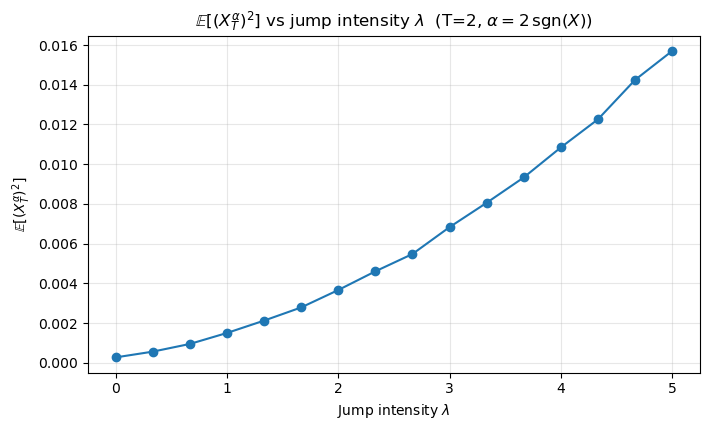
Figure 2. Dependence of 𝔼​[(XTα)2]\mathbb{E}[(X_{T}^{\alpha})^{2}] on (left) jump intensity λ\lambda and (right) jump-size standard deviation τ\tau for T=2T=2 under the feedback control αt=2​sgn​(Xt)\alpha_{t}=2\,\mathrm{sgn}(X_{t}).
Interpretation of Results.

Figure 1 compares the terminal second moment
𝔼​[(XTα)2]\mathbb{E}[(X_{T}^{\alpha})^{2}] under three feedback controls: αt=−Xt\alpha_{t}=-X_{t}, αt=−𝟏{Xt>2}\alpha_{t}=-\mathbf{1}_{\{X_{t}>2\}}, and the sign-based rule α^t=2​sgn​(Xt)\hat{\alpha}_{t}=2\,\mathrm{sgn}(X_{t}) (optimal). The latter yields the smallest second moment, reflecting its stronger stabilising effect. It reacts symmetrically to deviations from the target, while the linear feedback provides weaker correction and the threshold policy performs worst due to limited intervention.

Figure 2 shows that 𝔼​[(XTα)2]\mathbb{E}[(X_{T}^{\alpha})^{2}] increases with both the claim intensity λ\lambda and volatility τ\tau. Higher jump frequency or variability amplifies reserve fluctuations despite optimal control. This highlights the trade-off between control and jump risk, underscoring the need to account for claim statistics in control design.

5. Concluding remarks

In this paper, we have established a necessary and sufficient stochastic maximum principle for jump–diffusion systems with a piecewise Lipschitz drift coefficient. The analysis begins with an explicit representation of the first variation process, derived by combining Itô’s formula for jump–diffusions with standard stochastic integral estimates—namely the Burkholder–Davis–Gundy and Kunita inequalities—and the fact that the law of the SDE solution admits a density with respect to the Lebesgue measure.

To handle the discontinuity in the drift, we constructed a sequence of approximating control problems with smooth coefficients. Ekeland’s variational principle was then applied to obtain a sequence of adjoint processes, allowing us to derive the maximum principle in the limit. The framework accommodates drift functions of the form

b​(x,a)=b1​(x,a)+b2​(x)+b3​(x),b(x,a)=b_{1}(x,a)+b_{2}(x)+b_{3}(x),

where the discontinuity arises from b2b_{2}.

The present setting, however, does not encompass the case in which the insurer seeks to optimise a parameter β>0\beta>0 representing the magnitude of a fixed drain or injection in the model (2.4)–(2.5). In that context, the drift takes the form

b​(x,a)=b1​(x)+b2​(x)​b3​(a),b(x,a)=b_{1}(x)+b_{2}(x)b_{3}(a),

where b2b_{2} is piecewise Lipschitz (and expressible as the difference of two monotone functions), and b1b_{1} is continuously differentiable with bounded derivative and linear growth.

Appendix A Proof of preliminary results on SDEs with jumps and irregular drifts

Proof of Lemma 2.6.

To prove the Lemma, we proceed as in [26, 27]. We consider the function GG defined by:

G​(x)=x+∑k=1mαk​ϕ​(x−ξkc)​(x−ξk)​|x−ξk|,\displaystyle G(x)=x+\sum_{k=1}^{m}\alpha_{k}\phi(\frac{x-\xi_{k}}{c})(x-\xi_{k})|x-\xi_{k}|, (A.1)

with

ϕ​(u)={(1+u)3​(1−u)3 if ​|u|≤1,0 otherwise, \phi(u)=\Big\{\begin{array}[]{lll}(1+u)^{3}(1-u)^{3}&\text{ if }|u|\leq 1,\\ 0&\text{ otherwise, }\end{array}
ℝ\{0}∋αk=b​(ξk−)−b​(ξk+)2,k∈{1,…,m}\mathbb{R}\backslash\{0\}\ni\alpha_{k}=\frac{b(\xi_{k^{-}})-b(\xi_{k^{+}})}{2},\,\,\,k\in\{1,\ldots,m\}
(0,∞)∋c<min⁡(min1≤k≤m⁡16​|αk|,min1≤k≤m−1⁡ξk+1−ξk2).\displaystyle(0,\infty)\ni c<\min\big(\min_{1\leq k\leq m}\frac{1}{6|\alpha_{k}|},\min_{1\leq k\leq m-1}\frac{\xi_{k+1}-\xi_{k}}{2}\big). (A.2)

It can be shown that one may choose cc such that G′​(x)>0G^{\prime}(x)>0 for all x∈ℝx\in\mathbb{R}. Hence GG admits a global inverse G−1:ℝ↦ℝG^{-1}:\mathbb{R}\mapsto\mathbb{R}. Both GG and its inverse G−1G^{-1} are Lipschitz and G∈Cb1G\in C^{1}_{b} i.e., GG is continuously differentiable with bounded derivative. In particular, GG is Lipschitz since it is piecewise Lipschitz and continuous (see for example [14]).

Let Y=G​(X)Y=G(X) and Yn=G​(Xn)Y^{n}=G(X^{n}). The processes YtY_{t} and YtnY^{n}_{t} then satisfy, respectively, the following SDEs.

d​Ytx=b¯​(Ytx)​d​t+σ¯​(Ytx)​d​Bt+∫ℝ\{0}γ¯​(Ytx,z)​N​(d​z,d​t),t∈[0,T],Y0x=G​(x),\mathrm{d}Y^{x}_{t}=\bar{b}(Y^{x}_{t})\mathrm{d}t+\bar{\sigma}(Y^{x}_{t})\mathrm{d}B_{t}+\int_{\mathbb{R}\backslash\{0\}}\bar{\gamma}(Y^{x}_{t},z)N(\mathrm{d}z,\mathrm{d}t),t\in[0,T],Y^{x}_{0}=G(x), (A.3)

and

{d​Ytn,x=b¯n​(Ytn,x)​d​t+σ¯​(Ytn,x)​d​Bt+∫ℝ\{0}γ¯​(Ytn,x,z)​N​(d​z,d​t),t∈[0,T]Y0n,x=G​(x),\begin{cases}\mathrm{d}Y^{n,x}_{t}=\bar{b}_{n}(Y^{n,x}_{t})\mathrm{d}t+\bar{\sigma}(Y^{n,x}_{t})\mathrm{d}B_{t}+\int_{\mathbb{R}\backslash\{0\}}\bar{\gamma}(Y^{n,x}_{t},z)N(\mathrm{d}z,\mathrm{d}t),t\in[0,T]\\ Y^{n,x}_{0}=G(x),\end{cases} (A.4)

where

{b¯​(y)=G′​(G−1​(y))​b​(G−1​(y))+12​G′′​(G−1​(y)),b¯n​(y)=G′​(G−1​(y))​bn​(G−1​(y))+12​G′′​(G−1​(y)),σ¯​(y)=G′​(G−1​(y)),γ¯​(y,z)=G​(G−1​(y)+γ​(G−1​(y),z))−G​(G−1​(y))=G​(G−1​(y)+γ​(z))−y.\begin{cases}\bar{b}(y)=G^{\prime}(G^{-1}(y))b(G^{-1}(y))+\frac{1}{2}G^{\prime\prime}(G^{-1}(y)),\\ \bar{b}_{n}(y)=G^{\prime}(G^{-1}(y))b_{n}(G^{-1}(y))+\frac{1}{2}G^{\prime\prime}(G^{-1}(y)),\qquad\bar{\sigma}(y)=G^{\prime}(G^{-1}(y)),\\ \bar{\gamma}(y,z)=G(G^{-1}(y)+\gamma(G^{-1}(y),z))-G(G^{-1}(y))=G(G^{-1}(y)+\gamma(z))-y.\end{cases} (A.5)

Both b¯n\bar{b}_{n} and b¯\bar{b} are of at most linear growth, with b¯n​(x)→b¯​(x)\bar{b}_{n}(x)\rightarrow\bar{b}(x) for d​x\mathrm{d}x-a.e. xx. Moreover, [14] shows that b¯,σ¯\bar{b},\bar{\sigma} and, γ¯\bar{\gamma} are Lipschitz continuous and of at most linear growth; hence b¯n\bar{b}_{n} is also of at most linear growth and Lipschitz, with a Lipschitz constant independent of nn. It then follows from [24, Theorem 3] that the SDE (A.3) (respectively, (A.4)) admits a unique global strong solution. In addition the law of YtY_{t} has an absolute continuous density with respect to the Lebesgues measure (see Remark A.1).

Moreover, one has:

𝔼​[sup0≤s≤t|Ytx−Ytn,x|2]→0​ as ​n​ goes to ​∞\displaystyle\mathbb{E}\big[\sup_{0\leq s\leq t}|Y^{x}_{t}-Y^{n,x}_{t}|^{2}\big]\rightarrow 0\text{ as }n\text{ goes to }\infty (A.6)

Indeed, using Hölder, Burkholder-Davis-Gundy, Kunita’s and Gronwal’s inequlities, we have

𝔼​[sup0≤t≤T|Ytx−Ytn,x|2]\displaystyle\mathbb{E}\big[\sup_{0\leq t\leq T}|Y^{x}_{t}-Y^{n,x}_{t}|^{2}\big]
≤\displaystyle\leq 4​𝔼​[sup0≤t≤T|∫0t{b¯​(Ysx)−b¯n​(Ysn,x)}​ds|2]\displaystyle 4\mathbb{E}\big[\sup_{0\leq t\leq T}\big|\int_{0}^{t}\big\{\bar{b}(Y^{x}_{s})-\bar{b}_{n}(Y^{n,x}_{s})\big\}\mathrm{d}s\big|^{2}\big]
+𝔼​[sup0≤t≤T|∫0t{σ¯​(Ysx)−σ¯​(Ysn,x)}​dBs|2]\displaystyle+\mathbb{E}\big[\sup_{0\leq t\leq T}\big|\int_{0}^{t}\big\{\bar{\sigma}(Y^{x}_{s})-\bar{\sigma}(Y^{n,x}_{s})\big\}\mathrm{d}B_{s}\big|^{2}\big]
+𝔼​[sup0≤t≤T|∫0t∫ℝ\{0}{γ¯​(Ysx,z)−γ¯​(Ysn,x,z)}​N​(d​z,d​s)|2]\displaystyle+\mathbb{E}\big[\sup_{0\leq t\leq T}\big|\int_{0}^{t}\int_{\mathbb{R}\backslash\{0\}}\big\{\bar{\gamma}(Y^{x}_{s},z)-\bar{\gamma}(Y^{n,x}_{s},z)\big\}N(\mathrm{d}z,\mathrm{d}s)\big|^{2}\big]
≤\displaystyle\leq C​𝔼​[∫0T|b¯​(Ysx)−b¯n​(Ysx)+b¯n​(Ysx)−b¯n​(Ysn,x)|2​ds]\displaystyle C\mathbb{E}\big[\int_{0}^{T}\big|\bar{b}(Y^{x}_{s})-\bar{b}_{n}(Y^{x}_{s})+\bar{b}_{n}(Y^{x}_{s})-\bar{b}_{n}(Y^{n,x}_{s})\big|^{2}\mathrm{d}s\big]
+C​M​𝔼​[∫0T|Ysx−Ysn,x|2​ds]+C​M​𝔼​[∫0T∫ℝ\{0}|Ysx−Ysn,x|2​ν​(d​z)​ds]\displaystyle+CM\mathbb{E}\big[\int_{0}^{T}\big|Y^{x}_{s}-Y^{n,x}_{s}\big|^{2}\mathrm{d}s\big]+CM\mathbb{E}\big[\int_{0}^{T}\int_{\mathbb{R}\backslash\{0\}}\big|Y^{x}_{s}-Y^{n,x}_{s}\big|^{2}\nu(\mathrm{d}z)\mathrm{d}s\big]
≤\displaystyle\leq C​∫0T𝔼​[|b¯​(Ysx)−b¯n​(Ysx)|2]​ds,\displaystyle C\int_{0}^{T}\mathbb{E}\big[\big|\bar{b}(Y^{x}_{s})-\bar{b}_{n}(Y^{x}_{s})\big|^{2}\big]\mathrm{d}s, (A.7)

where CC is a constant that may change from one line to the other and we have use the uniform Lipschitz continuity of bnb_{n}.

Next since the law of YsY_{s} admits an absolute continuous density with respect to the Lebesgue measure, we have

∫0T𝔼​[|b¯​(Ysx)−b¯n​(Ysx)|2]​ds=∫0T∫ℝ|b¯​(y)−b¯n​(y)|2​φ​(y)​dy​ds\int_{0}^{T}\mathbb{E}\big[\big|\bar{b}(Y^{x}_{s})-\bar{b}_{n}(Y^{x}_{s})\big|^{2}\big]\mathrm{d}s=\int_{0}^{T}\int_{\mathbb{R}}\big|\bar{b}(y)-\bar{b}_{n}(y)\big|^{2}\varphi(y)\mathrm{d}y\mathrm{d}s

Moreover, the linear growth assumption ensures that

𝔼​[|b¯​(Ysx)−b¯n​(Ysx)|2]≤M​(1+𝔼​[|Ysx|2])≤MT​(1+|x|2)\mathbb{E}\big[\big|\bar{b}(Y^{x}_{s})-\bar{b}_{n}(Y^{x}_{s})\big|^{2}\Big]\leq M(1+\mathbb{E}\big[\big|Y^{x}_{s}\big|^{2}\big])\leq M_{T}(1+|x|^{2})

Thus the dominated convergence result yields (A.6). Finally

𝔼​[sup0≤s≤t|Xtx−Xtn,x|2]=\displaystyle\mathbb{E}\big[\sup_{0\leq s\leq t}|X^{x}_{t}-X^{n,x}_{t}|^{2}\big]= 𝔼​[sup0≤s≤t|G−1​(Ytx)−G−1​(Ytn,x)|2]\displaystyle\mathbb{E}\big[\sup_{0\leq s\leq t}|G^{-1}(Y^{x}_{t})-G^{-1}(Y^{n,x}_{t})|^{2}\big]
≤\displaystyle\leq M​𝔼​[sup0≤s≤t|Ytx−Ytn,x|2]→0​ as ​n​ goes to ​∞.\displaystyle M\mathbb{E}\big[\sup_{0\leq s\leq t}|Y^{x}_{t}-Y^{n,x}_{t}|^{2}\big]\rightarrow 0\text{ as }n\text{ goes to }\infty. (A.8)

∎

Remark A.1.

Note that cc in (A.2) can be chosen small enough to insure uniform ellipticity of the diffusion coefficient σ¯\bar{\sigma}. More precisely on can choose cc such that

0<g¯:=infx∈ℝG′(x)≤supx∈ℝG′(x)=:g¯<∞,G′′∈L∞(ℝ),0<\underline{g}:=\inf_{x\in\mathbb{R}}G^{\prime}(x)\leq\sup_{x\in\mathbb{R}}G^{\prime}(x)=:\overline{g}<\infty,\qquad G^{\prime\prime}\in L^{\infty}(\mathbb{R}), (A.9)

In addition, 1+γ¯y≠01+\bar{\gamma}_{y}\neq 0. As a consequence the law of the solution YtY_{t} (and thus XtX_{t}) to the SDE (A.3) has a density with respect to the Lebesgue measure (see for example [21, Theorem 11.4.4]).

Proof of Theorem 2.7.

It is easy to see that the first variation process exist. Indeed since the coefficient given in the SDE of YtxY^{x}_{t} are Lipschitz continuous, it follows from [11, Page 96 line before Sect. 3.4] that YtxY^{x}_{t} is differentiable with respect to the initial condition and we have:

∂Ytx∂x=\displaystyle\frac{\partial Y^{x}_{t}}{\partial x}= G′​(x)+∫0tb¯′​(Ysx)​∂Ysx∂x​ds+∫0tσ¯′​(Ysx)​∂Ysx∂x​dBs\displaystyle G^{\prime}(x)+\int_{0}^{t}\bar{b}^{\prime}(Y^{x}_{s})\frac{\partial Y^{x}_{s}}{\partial x}\mathrm{d}s+\int_{0}^{t}\bar{\sigma}^{\prime}(Y^{x}_{s})\frac{\partial Y^{x}_{s}}{\partial x}\mathrm{d}B_{s}
+∫0t∫ℝ\{0}γ¯′​(Ysx,z)​∂Ysx∂x​N​(d​z,d​s).\displaystyle+\int_{0}^{t}\int_{\mathbb{R}\backslash\{0\}}\bar{\gamma}^{\prime}(Y^{x}_{s},z)\frac{\partial Y^{x}_{s}}{\partial x}N(\mathrm{d}z,\mathrm{d}s). (A.10)

Since b¯′,σ¯′\bar{b}^{\prime},\bar{\sigma}^{\prime} and γ¯′\bar{\gamma}^{\prime} are bounded, it follows from [11, Theorem 3.3.1] that for all p≥2p\geq 2 𝔼​[|∂Ytx∂x|p]≤C\mathbb{E}\big[\big|\frac{\partial Y^{x}_{t}}{\partial x}\big|^{p}\big]\leq C. In addition, using the boundedness of b¯′,σ¯′,b¯n′\bar{b}^{\prime},\bar{\sigma}^{\prime},\bar{b}_{n}^{\prime} and γ¯′\bar{\gamma}^{\prime} and the fact that bn′​(x)b^{\prime}_{n}(x) converges to b′​(x),d​xb^{\prime}(x),\,\mathrm{d}x-a.e. one can show that

∂Ytn,x∂x→∂Ytx∂x​ strongly in ​L2​(Ω)\displaystyle\frac{\partial Y^{n,x}_{t}}{\partial x}\rightarrow\frac{\partial Y^{x}_{t}}{\partial x}\text{ strongly in }L^{2}(\Omega) (A.11)

Indeed

|∂Ytn,x∂x−∂Ytx∂x|2\displaystyle\big|\frac{\partial Y^{n,x}_{t}}{\partial x}-\frac{\partial Y^{x}_{t}}{\partial x}\big|^{2}
≤\displaystyle\leq 4​|∫0t(b¯n′​(Ysn,x)​∂Ysn,x∂x−b¯′​(Ysx)​∂Ysx∂x)​ds|2\displaystyle 4\big|\int_{0}^{t}\big(\bar{b}_{n}^{\prime}(Y^{n,x}_{s})\frac{\partial Y^{n,x}_{s}}{\partial x}-\bar{b}^{\prime}(Y^{x}_{s})\frac{\partial Y^{x}_{s}}{\partial x}\big)\mathrm{d}s\big|^{2}
+4​|∫0t(σ¯′​(Ysn,x)​∂Ysn,x∂x−σ′​(Ysx)​∂Ysx∂x)​dBs|2\displaystyle+4\big|\int_{0}^{t}\big(\bar{\sigma}^{\prime}(Y^{n,x}_{s})\frac{\partial Y^{n,x}_{s}}{\partial x}-\sigma^{\prime}(Y^{x}_{s})\frac{\partial Y^{x}_{s}}{\partial x}\big)\mathrm{d}B_{s}\big|^{2}
+4​|∫0t∫ℝ\{0}(γ¯′​(Ysn,x,z)​∂Ysn,x∂x−γ¯′​(Ysx,z)​∂Ysx∂x)​N​(d​z,d​s)|2\displaystyle+4\big|\int_{0}^{t}\int_{\mathbb{R}\backslash\{0\}}\big(\bar{\gamma}^{\prime}(Y^{n,x}_{s},z)\frac{\partial Y^{n,x}_{s}}{\partial x}-\bar{\gamma}^{\prime}(Y^{x}_{s},z)\frac{\partial Y^{x}_{s}}{\partial x}\big)N(\mathrm{d}z,\mathrm{d}s)\big|^{2}
≤\displaystyle\leq 8(|∫0t(b¯n′(Ysn,x)−b¯′(Ysx))∂Ysn,x∂xds|2+|∫0tb¯′(Ysx)(∂Ysn,x∂x−∂Ysx∂x)ds|2\displaystyle 8\big(\big|\int_{0}^{t}\big(\bar{b}_{n}^{\prime}(Y^{n,x}_{s})-\bar{b}^{\prime}(Y^{x}_{s})\big)\frac{\partial Y^{n,x}_{s}}{\partial x}\mathrm{d}s\big|^{2}+\big|\int_{0}^{t}\bar{b}^{\prime}(Y^{x}_{s})\big(\frac{\partial Y^{n,x}_{s}}{\partial x}-\frac{\partial Y^{x}_{s}}{\partial x}\big)\mathrm{d}s\big|^{2}
+|∫0t(σ¯′​(Ysn,x)−σ¯′​(Ysx))​∂Ysn,x∂x​dBs|2+|∫0tσ¯′​(Ysx)​(∂Ysn,x∂x−∂Ysx∂x)​dBs|2\displaystyle+\big|\int_{0}^{t}\big(\bar{\sigma}^{\prime}(Y^{n,x}_{s})-\bar{\sigma}^{\prime}(Y^{x}_{s})\big)\frac{\partial Y^{n,x}_{s}}{\partial x}\mathrm{d}B_{s}\big|^{2}+\big|\int_{0}^{t}\bar{\sigma}^{\prime}(Y^{x}_{s})\big(\frac{\partial Y^{n,x}_{s}}{\partial x}-\frac{\partial Y^{x}_{s}}{\partial x}\big)\mathrm{d}B_{s}\big|^{2}
+|∫0t∫ℝ\{0}(γ¯′​(Ysn,x,z)−γ¯′​(Ysx,z))​∂Ysn,x∂x​N​(d​z,d​s)|2\displaystyle+\big|\int_{0}^{t}\int_{\mathbb{R}\backslash\{0\}}\big(\bar{\gamma}^{\prime}(Y^{n,x}_{s},z)-\bar{\gamma}^{\prime}(Y^{x}_{s},z)\big)\frac{\partial Y^{n,x}_{s}}{\partial x}N(\mathrm{d}z,\mathrm{d}s)\big|^{2}
+|∫0t∫ℝ\{0}γ¯′(Ysx,z)(∂Ysn,x∂x−∂Ysx∂x)N(dz,ds)|2)\displaystyle+\big|\int_{0}^{t}\int_{\mathbb{R}\backslash\{0\}}\bar{\gamma}^{\prime}(Y^{x}_{s},z)\big(\frac{\partial Y^{n,x}_{s}}{\partial x}-\frac{\partial Y^{x}_{s}}{\partial x}\big)N(\mathrm{d}z,\mathrm{d}s)\big|^{2}\big)
≤\displaystyle\leq 8(∫0t|b¯n′(Ysn,x)−b¯′(Ysx)|2ds∫0t|∂Ysn,x∂x|2ds+M2∫0t|∂Ysn,x∂x−∂Ysx∂x|2ds\displaystyle 8\big(\int_{0}^{t}\big|\bar{b}_{n}^{\prime}(Y^{n,x}_{s})-\bar{b}^{\prime}(Y^{x}_{s})\big|^{2}\mathrm{d}s\int_{0}^{t}\big|\frac{\partial Y^{n,x}_{s}}{\partial x}\big|^{2}\mathrm{d}s+M^{2}\int_{0}^{t}\big|\frac{\partial Y^{n,x}_{s}}{\partial x}-\frac{\partial Y^{x}_{s}}{\partial x}\big|^{2}\mathrm{d}s
+|∫0t(σ¯′​(Ysn,x)−σ¯′​(Ysx))​∂Ysn,x∂x​dBs|2+|∫0tσ¯′​(Ysx)​(∂Ysn,x∂x−∂Ysx∂x)​dBs|2\displaystyle+\big|\int_{0}^{t}\big(\bar{\sigma}^{\prime}(Y^{n,x}_{s})-\bar{\sigma}^{\prime}(Y^{x}_{s})\big)\frac{\partial Y^{n,x}_{s}}{\partial x}\mathrm{d}B_{s}\big|^{2}+\big|\int_{0}^{t}\bar{\sigma}^{\prime}(Y^{x}_{s})\big(\frac{\partial Y^{n,x}_{s}}{\partial x}-\frac{\partial Y^{x}_{s}}{\partial x}\big)\mathrm{d}B_{s}\big|^{2}
+|∫0t∫ℝ\{0}(γ¯′​(Ysn,x,z)−γ¯′​(Ysx,z))​∂Ysn,x∂x​N​(d​z,d​s)|2\displaystyle+\big|\int_{0}^{t}\int_{\mathbb{R}\backslash\{0\}}\big(\bar{\gamma}^{\prime}(Y^{n,x}_{s},z)-\bar{\gamma}^{\prime}(Y^{x}_{s},z)\big)\frac{\partial Y^{n,x}_{s}}{\partial x}N(\mathrm{d}z,\mathrm{d}s)\big|^{2}
+|∫0t∫ℝ\{0}γ¯′(Ysx,z)(∂Ysn,x∂x−∂Ysx∂x)N(dz,ds)|2).\displaystyle+\big|\int_{0}^{t}\int_{\mathbb{R}\backslash\{0\}}\bar{\gamma}^{\prime}(Y^{x}_{s},z)\big(\frac{\partial Y^{n,x}_{s}}{\partial x}-\frac{\partial Y^{x}_{s}}{\partial x}\big)N(\mathrm{d}z,\mathrm{d}s)\big|^{2}\big).

Taking the expectation on both sides, using Itô’s isometry, Hölder inequality repeatedly and Gronwall’s lemma gives

𝔼​[|∂Ytn,x∂x−∂Ytx∂x|2]\displaystyle\mathbb{E}\big[\big|\frac{\partial Y^{n,x}_{t}}{\partial x}-\frac{\partial Y^{x}_{t}}{\partial x}\big|^{2}\big]
≤\displaystyle\leq 8(C(T)C𝔼[∫0t|b¯n′(Ysn,x)−b¯′(Ysx)|4ds]1/2+M2∫0t𝔼[|∂Ysn,x∂x−∂Ysx∂x|2]ds\displaystyle 8\big(C(T)C\mathbb{E}\big[\int_{0}^{t}\big|\bar{b}_{n}^{\prime}(Y^{n,x}_{s})-\bar{b}^{\prime}(Y^{x}_{s})\big|^{4}\mathrm{d}s\big]^{1/2}+M^{2}\int_{0}^{t}\mathbb{E}\big[\big|\frac{\partial Y^{n,x}_{s}}{\partial x}-\frac{\partial Y^{x}_{s}}{\partial x}\big|^{2}\big]\mathrm{d}s
+C​(T)​∫0t𝔼​[|σ¯′​(Ysn,x)−σ¯′​(Ysx)|4]1/2​ds+M2​∫0t𝔼​[|∂Ysn,x∂x−∂Ysx∂x|2]​ds\displaystyle+C(T)\int_{0}^{t}\mathbb{E}\big[\big|\bar{\sigma}^{\prime}(Y^{n,x}_{s})-\bar{\sigma}^{\prime}(Y^{x}_{s})\big|^{4}\big]^{1/2}\mathrm{d}s+M^{2}\int_{0}^{t}\mathbb{E}\big[\big|\frac{\partial Y^{n,x}_{s}}{\partial x}-\frac{\partial Y^{x}_{s}}{\partial x}\big|^{2}\big]\mathrm{d}s
+C​(T)​∫0t∫ℝ\{0}𝔼​[|γ¯′​(Ysn,x,z)−γ¯′​(Ysx,z)|4]1/2​ν​(d​z)​ds\displaystyle+C(T)\int_{0}^{t}\int_{\mathbb{R}\backslash\{0\}}\mathbb{E}\big[\big|\bar{\gamma}^{\prime}(Y^{n,x}_{s},z)-\bar{\gamma}^{\prime}(Y^{x}_{s},z)\big|^{4}\big]^{1/2}\nu(\mathrm{d}z)\mathrm{d}s
+M2∫0t∫ℝ\{0}𝔼[|∂Ysn,x∂x−∂Ysx∂x|2]ν(dz)ds)\displaystyle+M^{2}\int_{0}^{t}\int_{\mathbb{R}\backslash\{0\}}\mathbb{E}\big[\big|\frac{\partial Y^{n,x}_{s}}{\partial x}-\frac{\partial Y^{x}_{s}}{\partial x}\big|^{2}\big]\nu(\mathrm{d}z)\mathrm{d}s\big)
≤\displaystyle\leq 8C(T)eC​(T,M,ν)(𝔼[∫0T|b¯n′(Ysn,x)−b¯′(Ysx)|4ds]1/2\displaystyle 8C(T)e^{C(T,M,\nu)}\big(\mathbb{E}\big[\int_{0}^{T}\big|\bar{b}_{n}^{\prime}(Y^{n,x}_{s})-\bar{b}^{\prime}(Y^{x}_{s})\big|^{4}\mathrm{d}s\big]^{1/2}
+∫0T𝔼​[|σ¯′​(Ysn,x)−σ¯′​(Ysx)|2]1/2​ds\displaystyle+\int_{0}^{T}\mathbb{E}\big[\big|\bar{\sigma}^{\prime}(Y^{n,x}_{s})-\bar{\sigma}^{\prime}(Y^{x}_{s})\big|^{2}\big]^{1/2}\mathrm{d}s
+∫0T∫ℝ\{0}𝔼[|γ¯′(Ysn,x,z)−γ¯′(Ysx,z)|2]1/2ν(dz)ds).\displaystyle+\int_{0}^{T}\int_{\mathbb{R}\backslash\{0\}}\mathbb{E}\big[\big|\bar{\gamma}^{\prime}(Y^{n,x}_{s},z)-\bar{\gamma}^{\prime}(Y^{x}_{s},z)\big|^{2}\big]^{1/2}\nu(\mathrm{d}z)\mathrm{d}s\big).

Let us now show that the first term on the right side converges to 0.

∫0T𝔼​[|b¯n′​(Ysn,x)−b¯′​(Ysx)|4]​ds≤\displaystyle\int_{0}^{T}\mathbb{E}\big[\big|\bar{b}_{n}^{\prime}(Y^{n,x}_{s})-\bar{b}^{\prime}(Y^{x}_{s})\big|^{4}\big]\mathrm{d}s\leq ∫0T𝔼​[|b¯n′​(Ysn,x)−b¯′​(Ysn,x)|4]​ds\displaystyle\int_{0}^{T}\mathbb{E}\big[\big|\bar{b}_{n}^{\prime}(Y^{n,x}_{s})-\bar{b}^{\prime}(Y^{n,x}_{s})\big|^{4}\big]\mathrm{d}s
+∫0T𝔼​[|b¯′​(Ysn,x)−b¯′​(Ysx)|4]​ds\displaystyle+\int_{0}^{T}\mathbb{E}\big[\big|\bar{b}^{\prime}(Y^{n,x}_{s})-\bar{b}^{\prime}(Y^{x}_{s})\big|^{4}\big]\mathrm{d}s
=\displaystyle= ∫0T(I1,n​(t)+I2,n​(t))​dt\displaystyle\int_{0}^{T}(I_{1,n}(t)+I_{2,n}(t))\mathrm{d}t

Uniform linear growth of the coefficients of the SDE (A.4), yield by [11, Theorem 3.3.1] that (L3) in Lemma B.3 is satisfied. Combining Theorem B.2 and Lemma B.3 gives the convergence of ∫0TI1,n​(t)​dt\int_{0}^{T}I_{1,n}(t)\mathrm{d}t

To prove that limn→0∫0TI1,n​(t)​dt=0\lim\limits_{n\rightarrow 0}\int_{0}^{T}I_{1,n}(t)\mathrm{d}t=0, let k∈ℕk\in\mathbb{N} and consider the function b¯k′\bar{b}_{k}^{\prime} as in as in Lemma B.1

∫0TI1,n​(t)​dt≤\displaystyle\int_{0}^{T}I_{1,n}(t)\mathrm{d}t\leq C(∫0T𝔼[|b¯′(Ysn,x)−b¯k′(Ysn,x)|4]dt+∫0T𝔼[|b¯k′(Ysn,x)−b¯k′(Ysx)|4]dt\displaystyle C\big(\int_{0}^{T}\mathbb{E}\big[\big|\bar{b}^{\prime}(Y^{n,x}_{s})-\bar{b}_{k}^{\prime}(Y^{n,x}_{s})\big|^{4}\big]\mathrm{d}t+\int_{0}^{T}\mathbb{E}\big[\big|\bar{b}_{k}^{\prime}(Y^{n,x}_{s})-\bar{b}_{k}^{\prime}(Y^{x}_{s})\big|^{4}\big]\mathrm{d}t
+∫0T𝔼​[|b¯k′​(Ysx)−b¯′​(Ysx)|4]​dt=C​∫0T(I2,n1+I2,n2+I2,n3)​dt.\displaystyle+\int_{0}^{T}\mathbb{E}\big[\big|\bar{b}_{k}^{\prime}(Y^{x}_{s})-\bar{b}^{\prime}(Y^{x}_{s})\big|^{4}\big]\mathrm{d}t=C\int_{0}^{T}(I^{1}_{2,n}+I^{2}_{2,n}+I^{3}_{2,n})\mathrm{d}t. (A.12)

By arguments similar to those used in the proof of the convergence of ∫0TI1,n​(t)​dt\int_{0}^{T}I_{1,n}(t)\mathrm{d}t, we obtain that ∫0TI2,n1​dt\int_{0}^{T}I^{1}_{2,n}\mathrm{d}t and ∫0TI2,n3​dt\int_{0}^{T}I^{3}_{2,n}\mathrm{d}t converges to zero. The convergence of ∫0TI2,n2​dt\int_{0}^{T}I^{2}_{2,n}\mathrm{d}t follows from the continuity of bk′b^{\prime}_{k}, the fact that Ysn,x→YsxY^{n,x}_{s}\rightarrow Y^{x}_{s} uniformly in L2L^{2} (and hence in probability), and the dominated convergence theorem.

Moreover, since G−1G^{-1} is Lipschitz continuous, it follows that Xtx=G−1​(Ytx)X^{x}_{t}=G^{-1}(Y^{x}_{t}) is weakly differentiable with respect to the initial condition and we have

∂Xtn,x∂x=(G−1)′​(Ytn,x)​∂Ytn,x∂x→∂Xtx∂x=(G−1)′​(Ytx)​∂Ytn,x∂x​ strongly in ​L2​(Ω).\frac{\partial X^{n,x}_{t}}{\partial x}=(G^{-1})^{\prime}(Y^{n,x}_{t})\frac{\partial Y^{n,x}_{t}}{\partial x}\rightarrow\frac{\partial X^{x}_{t}}{\partial x}=(G^{-1})^{\prime}(Y^{x}_{t})\frac{\partial Y^{n,x}_{t}}{\partial x}\text{ strongly in }L^{2}(\Omega).

This follows as in the proof of the convergence of I2,nI_{2,n} in (A) using the fact that ∂Ytn,x∂x→∂Ytx∂x​ strongly in ​L2​(Ω)\frac{\partial Y^{n,x}_{t}}{\partial x}\rightarrow\frac{\partial Y^{x}_{t}}{\partial x}\text{ strongly in }L^{2}(\Omega), ∂Ytx∂x\frac{\partial Y^{x}_{t}}{\partial x} has all moments and that (G−1)′(G^{-1})^{\prime} is bounded.

Now, let us consider Xtn,xX^{n,x}_{t}, the solution to the SDE (LABEL:eq:SDErvmain1n). As mentioned above, Xtn,xX^{n,x}_{t} is differentiable with respect to the initial condition. Next we show that its derivative satisfies a linear stochastic differential equation given by

∂Xtx,n∂x=\displaystyle\frac{\partial X^{x,n}_{t}}{\partial x}= 1+∫0t(b1′​(Xux,n)+b2,n′​(Xux,n))​∂Xux,n∂x​du\displaystyle 1+\int_{0}^{t}\big(b^{\prime}_{1}(X^{x,n}_{u})+b^{\prime}_{2,n}(X^{x,n}_{u})\big)\frac{\partial X^{x,n}_{u}}{\partial x}\mathrm{d}u
=\displaystyle= exp⁡{∫0t(b1′​(Xux,n)+b2,n′​(Xux,n))​du}.\displaystyle\exp\big\{\int_{0}^{t}\big(b^{\prime}_{1}(X^{x,n}_{u})+b^{\prime}_{2,n}(X^{x,n}_{u})\big)\mathrm{d}u\big\}.

Now set b~2,n​(x)=∫−∞xb2,n​(y)​dy.\tilde{b}_{2,n}(x)=\int_{-\infty}^{x}b_{2,n}(y)\mathrm{d}y. Then by Itô’s formula for Lévy processes, one has:

b~2,n​(Xtn,x)−b~2,n​(x)\displaystyle\tilde{b}_{2,n}(X^{n,x}_{t})-\tilde{b}_{2,n}(x)
=\displaystyle= ∫0tb1​(Xun,x)​b2​(Xun,x)​du+∫0tb2,n2​(Xun,x)​du+∫0tb2,n​(Xun,x)​dBu\displaystyle\int_{0}^{t}b_{1}(X^{n,x}_{u})b_{2}(X^{n,x}_{u})\mathrm{d}u+\int_{0}^{t}b^{2}_{2,n}(X^{n,x}_{u})\mathrm{d}u+\int_{0}^{t}b_{2,n}(X^{n,x}_{u})\mathrm{d}B_{u}
+12​∫0tb2,n′​(Xun,x)​du+∫0t∫ℝ\{0}{b~2,n​(Xun,x+γ​(z))−b~2,n​(Xun,x)}​N​(d​z,d​u)\displaystyle+\frac{1}{2}\int_{0}^{t}b^{\prime}_{2,n}(X^{n,x}_{u})\mathrm{d}u+\int_{0}^{t}\int_{\mathbb{R}\backslash\{0\}}\big\{\tilde{b}_{2,n}(X^{n,x}_{u}+\gamma(z))-\tilde{b}_{2,n}(X^{n,x}_{u})\big\}N(\mathrm{d}z,\mathrm{d}u)

Substituting this above gives

∂Xtx,n∂x=\displaystyle\frac{\partial X^{x,n}_{t}}{\partial x}= exp{∫0tb1′(Xux,n)du+2(b~2,n(Xtn,x)−b~2,n(x)−∫0tb2,n2(Xun,x)du\displaystyle\exp\big\{\int_{0}^{t}b^{\prime}_{1}(X^{x,n}_{u})\mathrm{d}u+2\big(\tilde{b}_{2,n}(X^{n,x}_{t})-\tilde{b}_{2,n}(x)-\int_{0}^{t}b^{2}_{2,n}(X^{n,x}_{u})\mathrm{d}u
−∫0tb1​(Xun,x)​b2​(Xun,x)​du−∫0tb2,n​(Xun,x)​dBu\displaystyle-\int_{0}^{t}b_{1}(X^{n,x}_{u})b_{2}(X^{n,x}_{u})\mathrm{d}u-\int_{0}^{t}b_{2,n}(X^{n,x}_{u})\mathrm{d}B_{u}
−∫0t∫ℝ\{0}{b~2,n(Xun,x+γ(z))−b~2,n(Xun,x)}N(dz,du))}\displaystyle-\int_{0}^{t}\int_{\mathbb{R}\backslash\{0\}}\big\{\tilde{b}_{2,n}(X^{n,x}_{u}+\gamma(z))-\tilde{b}_{2,n}(X^{n,x}_{u})\big\}N(\mathrm{d}z,\mathrm{d}u)\big)\big\}

Claim 1 We claim that the right side of the above converges strongly in L2L^{2} to the right side of (2.7).

Proof of Claim 1.
𝔼[|exp{∫0tb1′(Xux,n)du+2(b~2,n(Xtn,x)−b~2,n(x)−∫0tb2,n(Xun,x)dBudu\displaystyle\mathbb{E}\Big[\Big|\exp\big\{\int_{0}^{t}b^{\prime}_{1}(X^{x,n}_{u})\mathrm{d}u+2\big(\tilde{b}_{2,n}(X^{n,x}_{t})-\tilde{b}_{2,n}(x)-\int_{0}^{t}b_{2,n}(X^{n,x}_{u})\mathrm{d}B_{u}\mathrm{d}u
−2​∫0tb2,n2​(Xux)−∫0tb1​(Xun,x)​b2​(Xun,x)​du\displaystyle-2\int_{0}^{t}b_{2,n}^{2}(X^{x}_{u})-\int_{0}^{t}b_{1}(X^{n,x}_{u})b_{2}(X^{n,x}_{u})\mathrm{d}u
−∫0t∫ℝ\{0}{b~2,n(Xun,x+γ(z))−b~2,n(Xun,x)}N(dz,du))}\displaystyle-\int_{0}^{t}\int_{\mathbb{R}\backslash\{0\}}\big\{\tilde{b}_{2,n}(X^{n,x}_{u}+\gamma(z))-\tilde{b}_{2,n}(X^{n,x}_{u})\big\}N(\mathrm{d}z,\mathrm{d}u)\big)\big\}
−exp{∫0tb1′(Xux)du+2(b~2(Xtx)−b~2(x)−∫0tb22(Xux)du−∫0tb2(Xux)dBu\displaystyle-\exp\big\{\int_{0}^{t}b_{1}^{\prime}(X^{x}_{u})\mathrm{d}u+2\big(\tilde{b}_{2}(X^{x}_{t})-\tilde{b}_{2}(x)-\int_{0}^{t}b_{2}^{2}(X^{x}_{u})\mathrm{d}u-\int_{0}^{t}b_{2}(X^{x}_{u})\mathrm{d}B_{u}
−∫0tb1(Xux)b2(Xux)du−∫0t∫ℝ\{0}{b~2(Xux+γ(z))−b~2(Xux)}N(dz,du))}|2]\displaystyle-\int_{0}^{t}b_{1}(X^{x}_{u})b_{2}(X^{x}_{u})\mathrm{d}u-\int_{0}^{t}\int_{\mathbb{R}\backslash\{0\}}\big\{\tilde{b}_{2}(X^{x}_{u}+\gamma(z))-\tilde{b}_{2}(X^{x}_{u})\big\}N(\mathrm{d}z,\mathrm{d}u)\big)\big\}\Big|^{2}\Big]
≤\displaystyle\leq 𝔼[|∫0t(b1′(Xux,n)−b1′(Xux))du−2(b~2,n(x)−b~2(x))+2(b~2,n(Xtn,x)−b~2(Xtx))\displaystyle\mathbb{E}\Big[\Big|\int_{0}^{t}\big(b^{\prime}_{1}(X^{x,n}_{u})-b_{1}^{\prime}(X^{x}_{u})\big)\mathrm{d}u-2\big(\tilde{b}_{2,n}(x)-\tilde{b}_{2}(x)\big)+2\big(\tilde{b}_{2,n}(X^{n,x}_{t})-\tilde{b}_{2}(X^{x}_{t})\big)
−2​∫0t(b2,n​(Xun,x)−b2​(Xux))​dBu−2​∫0t(b2,n2​(Xun,x)−b22​(Xux))​du\displaystyle-2\int_{0}^{t}\big(b_{2,n}(X^{n,x}_{u})-b_{2}(X^{x}_{u})\big)\mathrm{d}B_{u}-2\int_{0}^{t}\big(b^{2}_{2,n}(X^{n,x}_{u})-b_{2}^{2}(X^{x}_{u})\big)\mathrm{d}u
−2∫0t(b1(Xun,x)b2(Xun,x)−b1(Xux)b2(Xux))du−2∫0t∫ℝ\{0}{b~2,n(Xun,x+γ(z))\displaystyle-2\int_{0}^{t}\big(b_{1}(X^{n,x}_{u})b_{2}(X^{n,x}_{u})-b_{1}(X^{x}_{u})b_{2}(X^{x}_{u})\big)\mathrm{d}u-2\int_{0}^{t}\int_{\mathbb{R}\backslash\{0\}}\big\{\tilde{b}_{2,n}(X^{n,x}_{u}+\gamma(z))
−b~2,n(Xun,x)−b~2(Xux+γ(z))+b~2(Xux)}N(dz,du)\displaystyle-\tilde{b}_{2,n}(X^{n,x}_{u})-\tilde{b}_{2}(X^{x}_{u}+\gamma(z))+\tilde{b}_{2}(X^{x}_{u})\big\}N(\mathrm{d}z,\mathrm{d}u)
×|exp{∫0tb1′(Xux,n)du+2(b~2,n(Xtn,x)−b2,n(x)−∫0tb2,n(Xun,x)dBu\displaystyle\times\Big|\exp\big\{\int_{0}^{t}b^{\prime}_{1}(X^{x,n}_{u})\mathrm{d}u+2\big(\tilde{b}_{2,n}(X^{n,x}_{t})-b_{2,n}(x)-\int_{0}^{t}b_{2,n}(X^{n,x}_{u})\mathrm{d}B_{u}
−2​∫0tb2,n2​(Xux)​du−∫0tb1​(Xun,x)​b2​(Xun,x)​du\displaystyle-2\int_{0}^{t}b_{2,n}^{2}(X^{x}_{u})\mathrm{d}u-\int_{0}^{t}b_{1}(X^{n,x}_{u})b_{2}(X^{n,x}_{u})\mathrm{d}u
−∫0t∫ℝ\{0}{b~2,n(Xun,x+γ(z))−b~2,n(Xun,x)}N(dz,du))}\displaystyle-\int_{0}^{t}\int_{\mathbb{R}\backslash\{0\}}\big\{\tilde{b}_{2,n}(X^{n,x}_{u}+\gamma(z))-\tilde{b}_{2,n}(X^{n,x}_{u})\big\}N(\mathrm{d}z,\mathrm{d}u)\big)\big\}
+exp{∫0tb1′(Xux)du+2(b~2(Xtx)−b~2(x)−∫0tb22(Xux)du−∫0tb2(Xux)dBu\displaystyle+\exp\big\{\int_{0}^{t}b_{1}^{\prime}(X^{x}_{u})\mathrm{d}u+2\big(\tilde{b}_{2}(X^{x}_{t})-\tilde{b}_{2}(x)-\int_{0}^{t}b_{2}^{2}(X^{x}_{u})\mathrm{d}u-\int_{0}^{t}b_{2}(X^{x}_{u})\mathrm{d}B_{u}
−∫0tb1(Xux)b2(Xux)du−∫0t∫ℝ\{0}{b~2(Xux+γ(z))−b~2(Xux)}N(dz,du))}|2]\displaystyle-\int_{0}^{t}b_{1}(X^{x}_{u})b_{2}(X^{x}_{u})\mathrm{d}u-\int_{0}^{t}\int_{\mathbb{R}\backslash\{0\}}\big\{\tilde{b}_{2}(X^{x}_{u}+\gamma(z))-\tilde{b}_{2}(X^{x}_{u})\big\}N(\mathrm{d}z,\mathrm{d}u)\big)\big\}\Big|^{2}\Big]
=\displaystyle= 𝔼[ℐ1,n+ℐ2,n+ℐ3,n+ℐ4,n+ℐ5,n+ℐ6,n+ℐ7,n|2|𝒿1,n+𝒥2|2]\displaystyle\mathbb{E}\big[\mathcal{I}_{1,n}+\mathcal{I}_{2,n}+\mathcal{I}_{3,n}+\mathcal{I}_{4,n}+\mathcal{I}_{5,n}+\mathcal{I}_{6,n}+\mathcal{I}_{7,n}|^{2}|\mathcal{j}_{1,n}+\mathcal{J}_{2}|^{2}\big]
≤\displaystyle\leq C(𝔼[|ℐ1,n4]1/2+𝔼[|ℐ2,n|4]1/2+𝔼[|ℐ3,n|4]1/2+𝔼[|ℐ4,n|4]1/2+𝔼[|ℐ5,n|4]1/2\displaystyle C\Big(\mathbb{E}\big[|\mathcal{I}^{4}_{1,n}\big]^{1/2}+\mathbb{E}\big[|\mathcal{I}_{2,n}|^{4}\big]^{1/2}+\mathbb{E}\big[|\mathcal{I}_{3,n}|^{4}\big]^{1/2}+\mathbb{E}\big[|\mathcal{I}_{4,n}|^{4}\big]^{1/2}+\mathbb{E}\big[|\mathcal{I}_{5,n}|^{4}\big]^{1/2}
+𝔼[|ℐ6,n|4]1/2]1/2+𝔼[|ℐ7,n|4]1/2]1/2)(𝔼[|𝒥1,n|4]1/2+𝔼[|𝒥2|4]1/2).\displaystyle+\mathbb{E}\big[|\mathcal{I}_{6,n}|^{4}\big]^{1/2}\big]^{1/2}+\mathbb{E}\big[|\mathcal{I}_{7,n}|^{4}\big]^{1/2}\big]^{1/2}\Big)\Big(\mathbb{E}\big[|\mathcal{J}_{1,n}|^{4}\big]^{1/2}+\mathbb{E}\big[|\mathcal{J}_{2}|^{4}\big]^{1/2}\Big).

The convergence follows if we can show that the first seven terms converge to 0 whereas the last two terms are uniformly bounded. Let us for example look at the term 𝔼[ℐ4,n|4]\mathbb{E}\big[\mathcal{I}_{4,n}|^{4}\big]. Using Burkholder-Davis-Gundy and Hölder inequalities, we obtain

𝔼​[|ℐ4,n|4]=\displaystyle\mathbb{E}\big[|\mathcal{I}_{4,n}|^{4}\big]= 𝔼​[|∫0t(b2,n​(Xun,x)−b2​(Xux))​dBu|4]\displaystyle\mathbb{E}\big[\big|\int_{0}^{t}\big(b_{2,n}(X^{n,x}_{u})-b_{2}(X^{x}_{u})\big)\mathrm{d}B_{u}\big|^{4}\big]
≤\displaystyle\leq C​𝔼​[∫0t|b2,n​(Xun,x)−b2​(Xux)|4​du]\displaystyle C\mathbb{E}\big[\int_{0}^{t}\big|b_{2,n}(X^{n,x}_{u})-b_{2}(X^{x}_{u})\big|^{4}\mathrm{d}u\big]

Observe that Xtn,x=G−1​(Ytn,x)X^{n,x}_{t}=G^{-1}(Y^{n,x}_{t}) with G−1G^{-1} at most linear growth and G′G^{\prime} uniformly bounded. Thus assumptions of Lemma B.3 are satisfied and therefore, 𝔼​[|ℐ4,n|4]\mathbb{E}\big[|\mathcal{I}_{4,n}|^{4}\big] converges to 0. As for the term I7,nI_{7,n}, we have by using the linear growth of b~2,n,b~2\tilde{b}_{2,n},\tilde{b}_{2} and [11, Proposition 2.6.1] (see also [1, Theorem 4.4.23]).

𝔼​[|ℐ7,n|4]\displaystyle\mathbb{E}\big[|\mathcal{I}_{7,n}|^{4}\big]
=\displaystyle= 𝔼[|∫0t∫ℝ\{0}(b~2,n(Xun,x+γ(z))−b~2,n(Xun,x)−b~2(Xux+γ(z))\displaystyle\mathbb{E}\big[\big|\int_{0}^{t}\int_{\mathbb{R}\backslash\{0\}}\big(\tilde{b}_{2,n}(X^{n,x}_{u}+\gamma(z))-\tilde{b}_{2,n}(X^{n,x}_{u})-\tilde{b}_{2}(X^{x}_{u}+\gamma(z))
+b~2(Xux))N(dz,du)|4]\displaystyle+\tilde{b}_{2}(X^{x}_{u})\big)N(\mathrm{d}z,\mathrm{d}u)\big|^{4}\big]
≤\displaystyle\leq 𝔼[|∫0t∫ℝ\{0}(b~2,n(Xun,x+γ(z))−b~2,n(Xun,x)−b~2(Xux+γ(z))\displaystyle\mathbb{E}\big[\big|\int_{0}^{t}\int_{\mathbb{R}\backslash\{0\}}\big(\tilde{b}_{2,n}(X^{n,x}_{u}+\gamma(z))-\tilde{b}_{2,n}(X^{n,x}_{u})-\tilde{b}_{2}(X^{x}_{u}+\gamma(z))
+b~2(Xux))N(dz,du)|2]×𝔼[|∫0t∫ℝ\{0}(b~2,n(Xun,x+γ(z))−b~2,n(Xun,x)\displaystyle+\tilde{b}_{2}(X^{x}_{u})\big)N(\mathrm{d}z,\mathrm{d}u)\big|^{2}\big]\times\mathbb{E}\big[\big|\int_{0}^{t}\int_{\mathbb{R}\backslash\{0\}}\big(\tilde{b}_{2,n}(X^{n,x}_{u}+\gamma(z))-\tilde{b}_{2,n}(X^{n,x}_{u})
−b~2(Xux+γ(z))+b~2(Xux))N(dz,du)|6]\displaystyle-\tilde{b}_{2}(X^{x}_{u}+\gamma(z))+\tilde{b}_{2}(X^{x}_{u})\big)N(\mathrm{d}z,\mathrm{d}u)\big|^{6}\big]
≤\displaystyle\leq C∫0t∫ℝ\{0}𝔼[|b~2,n(Xun,x+γ(z))−b~2,n(Xun,x)−b~2(Xux+γ(z))\displaystyle C\int_{0}^{t}\int_{\mathbb{R}\backslash\{0\}}\mathbb{E}\big[\big|\tilde{b}_{2,n}(X^{n,x}_{u}+\gamma(z))-\tilde{b}_{2,n}(X^{n,x}_{u})-\tilde{b}_{2}(X^{x}_{u}+\gamma(z))
+b~2(Xux)|2]ν(dz)du×(∫0t∫ℝ\{0}𝔼[|b~2,n(Xun,x+γ(z))−b~2,n(Xun,x)\displaystyle+\tilde{b}_{2}(X^{x}_{u})\big|^{2}\big]\nu(\mathrm{d}z)\mathrm{d}u\times\Big(\int_{0}^{t}\int_{\mathbb{R}\backslash\{0\}}\mathbb{E}\big[\big|\tilde{b}_{2,n}(X^{n,x}_{u}+\gamma(z))-\tilde{b}_{2,n}(X^{n,x}_{u})
−b~2(Xux+γ(z))+b~2(Xux)|6]ν(dz)du×𝔼[(∫0t∫ℝ\{0}|b~2,n(Xun,x+γ(z))\displaystyle-\tilde{b}_{2}(X^{x}_{u}+\gamma(z))+\tilde{b}_{2}(X^{x}_{u})\big|^{6}\big]\nu(\mathrm{d}z)\mathrm{d}u\times\mathbb{E}\big[\big(\int_{0}^{t}\int_{\mathbb{R}\backslash\{0\}}\big|\tilde{b}_{2,n}(X^{n,x}_{u}+\gamma(z))
−b~2,n(Xun,x)−b~2(Xux+γ(z))+b~2(Xux)|2ν(dz)du)3])\displaystyle-\tilde{b}_{2,n}(X^{n,x}_{u})-\tilde{b}_{2}(X^{x}_{u}+\gamma(z))+\tilde{b}_{2}(X^{x}_{u})\big|^{2}\nu(\mathrm{d}z)\mathrm{d}u\big)^{3}\big]\Big)
≤\displaystyle\leq C​∫0t∫ℝ\{0}𝔼​[|∫01{b2,n​(Xun,x+λ​γ​(z))​Xun,x−b2​(Xux+λ​γ​(z))​Xux}​dλ|2]\displaystyle C\int_{0}^{t}\int_{\mathbb{R}\backslash\{0\}}\mathbb{E}\big[\big|\int_{0}^{1}\big\{b_{2,n}(X^{n,x}_{u}+\lambda\gamma(z))X^{n,x}_{u}-b_{2}(X^{x}_{u}+\lambda\gamma(z))X^{x}_{u}\big\}\mathrm{d}\lambda\big|^{2}\big]
γ2(z)ν(dz)du×(∫0t∫ℝ\{0}𝔼[|∫01{b2,n(Xun,x+λγ(z))Xun,x\displaystyle\gamma^{2}(z)\nu(\mathrm{d}z)\mathrm{d}u\times\Big(\int_{0}^{t}\int_{\mathbb{R}\backslash\{0\}}\mathbb{E}\big[\big|\int_{0}^{1}\big\{b_{2,n}(X^{n,x}_{u}+\lambda\gamma(z))X^{n,x}_{u}
−b2(Xux+λγ(z))Xux}dλ|6]γ6(z)ν(dz)du\displaystyle-b_{2}(X^{x}_{u}+\lambda\gamma(z))X^{x}_{u}\big\}\mathrm{d}\lambda\big|^{6}\big]\gamma^{6}(z)\nu(\mathrm{d}z)\mathrm{d}u
×𝔼[(∫0t∫ℝ\{0}|∫01{b2,n(Xun,x+λγ(z))Xun,x−b2(Xux+λγ(z))Xux}dλ|2\displaystyle\times\mathbb{E}\big[\big(\int_{0}^{t}\int_{\mathbb{R}\backslash\{0\}}\big|\int_{0}^{1}\big\{b_{2,n}(X^{n,x}_{u}+\lambda\gamma(z))X^{n,x}_{u}-b_{2}(X^{x}_{u}+\lambda\gamma(z))X^{x}_{u}\big\}\mathrm{d}\lambda\big|^{2}
γ2(z)ν(dz)du)3])\displaystyle\gamma^{2}(z)\nu(\mathrm{d}z)\mathrm{d}u\big)^{3}\big]\Big)
≤\displaystyle\leq C∫0t∫ℝ\{0}∫01(𝔼[|b2,n(Xun,x+λγ(z))−b2(Xux+λγ(z))|4]1/2𝔼[|Xun,x|4]1/2\displaystyle C\int_{0}^{t}\int_{\mathbb{R}\backslash\{0\}}\int_{0}^{1}\Big(\mathbb{E}\big[\big|b_{2,n}(X^{n,x}_{u}+\lambda\gamma(z))-b_{2}(X^{x}_{u}+\lambda\gamma(z))\big|^{4}\big]^{1/2}\mathbb{E}\big[\big|X^{n,x}_{u}\big|^{4}\big]^{1/2}
+𝔼[|b2(Xux+λγ(z))Xux|8]1/8𝔼[|Xun,x|4+|Xux|4]1/4𝔼[|Xun,x−Xux|2]1/2)\displaystyle+\mathbb{E}\big[\big|b_{2}(X^{x}_{u}+\lambda\gamma(z))X^{x}_{u}\big|^{8}\big]^{1/8}\mathbb{E}\big[\big|X^{n,x}_{u}\big|^{4}+\big|X^{x}_{u}\big|^{4}\big]^{1/4}\mathbb{E}\big[\big|X^{n,x}_{u}-X^{x}_{u}\big|^{2}\big]^{1/2}\Big)
dλγ2(z)ν(dz)du×(∫0t∫ℝ\{0}∫01𝔼[|Xun,x|6]+𝔼[|Xux|6]dλγ6(z)ν(dz)du\displaystyle\mathrm{d}\lambda\gamma^{2}(z)\nu(\mathrm{d}z)\mathrm{d}u\times\Big(\int_{0}^{t}\int_{\mathbb{R}\backslash\{0\}}\int_{0}^{1}\mathbb{E}\big[\big|X^{n,x}_{u}\big|^{6}\big]+\mathbb{E}\big[\big|X^{x}_{u}\big|^{6}\big]\mathrm{d}\lambda\gamma^{6}(z)\nu(\mathrm{d}z)\mathrm{d}u
×𝔼[(∫0t∫ℝ\{0}∫01(|Xun,x|2+|Xux|2)dλγ2(z)ν(dz)du)3])\displaystyle\times\mathbb{E}\big[\big(\int_{0}^{t}\int_{\mathbb{R}\backslash\{0\}}\int_{0}^{1}\big(\big|X^{n,x}_{u}|^{2}+\big|X^{x}_{u}\big|^{2}\big)\mathrm{d}\lambda\gamma^{2}(z)\nu(\mathrm{d}z)\mathrm{d}u\big)^{3}\big]\Big)
≤\displaystyle\leq C∫0t∫ℝ\{0}∫01(𝔼[|b2,n(Xun,x+λγ(z))−b2(Xux+λγ(z))|4]1/2\displaystyle C\int_{0}^{t}\int_{\mathbb{R}\backslash\{0\}}\int_{0}^{1}\Big(\mathbb{E}\big[\big|b_{2,n}(X^{n,x}_{u}+\lambda\gamma(z))-b_{2}(X^{x}_{u}+\lambda\gamma(z))\big|^{4}\big]^{1/2}
+𝔼[|Xun,x−Xux|2]1/2)dλγ2(z)ν(dz)du×∫0t∫ℝ\{0}𝔼[|Xun,x|6]+𝔼[|Xux|6]\displaystyle+\mathbb{E}\big[\big|X^{n,x}_{u}-X^{x}_{u}\big|^{2}\big]^{1/2}\Big)\mathrm{d}\lambda\gamma^{2}(z)\nu(\mathrm{d}z)\mathrm{d}u\times\int_{0}^{t}\int_{\mathbb{R}\backslash\{0\}}\mathbb{E}\big[\big|X^{n,x}_{u}\big|^{6}\big]+\mathbb{E}\big[\big|X^{x}_{u}\big|^{6}\big]
×γ6​(z)​ν​(d​z)​d​u×𝔼​[(∫0t∫ℝ\{0}(|Xun,x|2+|Xux|2)​γ2​(z)​ν​(d​z)​du)3]\displaystyle\times\gamma^{6}(z)\nu(\mathrm{d}z)\mathrm{d}u\times\mathbb{E}\big[\big(\int_{0}^{t}\int_{\mathbb{R}\backslash\{0\}}\big(\big|X^{n,x}_{u}|^{2}+\big|X^{x}_{u}\big|^{2}\big)\gamma^{2}(z)\nu(\mathrm{d}z)\mathrm{d}u\big)^{3}\big]
≤\displaystyle\leq C​(ℐ7,n1+ℐ7,n2)\displaystyle C(\mathcal{I}^{1}_{7,n}+\mathcal{I}^{2}_{7,n})

Here we have used the mean value theorem, the uniform boundedness of b~2,n′\tilde{b}^{\prime}_{2,n} and b~2′\tilde{b}^{\prime}_{2}, the fact that XuxX^{x}_{u} and Xun,xX^{n,x}_{u} have moments of all order uniformly in nn, together with the bound ∫ℝ\{0}γp​(z)​ν​(d​z)<∞\int_{\mathbb{R}\backslash\{0\}}\gamma^{p}(z)\nu(\mathrm{d}z)<\infty for p≥2p\geq 2. The convergence of ℐ7,n1\mathcal{I}^{1}_{7,n} follows from Lemma B.3 , while that of ℐ7,n2\mathcal{I}^{2}_{7,n} follows from strong convergence of Xun,xX^{n,x}_{u} to XuxX^{x}_{u} in L2​(Ω)L^{2}(\Omega).

The convergence of the derivative can be established by showing that all moments of 𝒥1,n\mathcal{J}_{1,n} are uniformly bounded; that is, sup𝑛​𝔼​[|𝒥1,n|p]<∞\underset{n}{\sup}\mathbb{E}[|\mathcal{J}_{1,n}|^{p}]<\infty for all p≥1p\geq 1. Indeed, taking the pp-power, taking the expectation and applying Hölder inequality, together with the properties of stochastic integral, the uniform boundedness of b2,nb_{2,n}, and the uniform Lipschitz continuity and uniform linear growth condition of b~2,n\tilde{b}_{2,n}, we have

𝔼​[|𝒥1,n|p]\displaystyle\mathbb{E}\big[\big|\mathcal{J}_{1,n}\big|^{p}\big]
≤\displaystyle\leq e−2​p​b~2,n​(x)​𝔼​[exp⁡{5​p​∫0tb1′​(Xux,n)​du}]1/5​𝔼​[exp⁡{10​p​b~2,n​(Xtn,x)}]1/5\displaystyle e^{-2p\tilde{b}_{2,n}(x)}\mathbb{E}\big[\exp\big\{5p\int_{0}^{t}b^{\prime}_{1}(X^{x,n}_{u})\mathrm{d}u\big\}\big]^{1/5}\mathbb{E}\big[\exp\big\{10p\tilde{b}_{2,n}(X^{n,x}_{t})\big\}\big]^{1/5}
×𝔼​[exp⁡{−10​p​∫0tb2,n2​(Xux)​du}]1/5​𝔼​[exp⁡{−10​p​∫0tb2,n​(Xun,x)​dBu}]1/5\displaystyle\times\mathbb{E}\big[\exp\big\{-10p\int_{0}^{t}b_{2,n}^{2}(X^{x}_{u})\mathrm{d}u\big\}\big]^{1/5}\mathbb{E}\big[\exp\big\{-10p\int_{0}^{t}b_{2,n}(X^{n,x}_{u})\mathrm{d}B_{u}\big\}\big]^{1/5}
×𝔼​[exp⁡{−10​p​∫0t∫ℝ\{0}{b~2,n​(Xun,x+γ​(z))−b~2,n​(Xun,x)}​N​(d​z,d​u)}]1/5\displaystyle\times\mathbb{E}\big[\exp\big\{-10p\int_{0}^{t}\int_{\mathbb{R}\backslash\{0\}}\big\{\tilde{b}_{2,n}(X^{n,x}_{u}+\gamma(z))-\tilde{b}_{2,n}(X^{n,x}_{u})\big\}N(\mathrm{d}z,\mathrm{d}u)\big\}\big]^{1/5}
≤\displaystyle\leq e2​M​P​(1+|x|)​C​(p)​𝔼​[exp⁡{10​p​M​(1+|Xtn,x|)}]1/5​𝔼​[exp⁡{50​p2​∫0tb2,n2​(Xun,x)​du}]1/5\displaystyle e^{2MP(1+|x|)}C(p)\mathbb{E}\big[\exp\big\{10pM(1+|X^{n,x}_{t}|)\big\}\big]^{1/5}\mathbb{E}\big[\exp\big\{50p^{2}\int_{0}^{t}b^{2}_{2,n}(X^{n,x}_{u})\mathrm{d}u\big\}\big]^{1/5}
×𝔼​[exp⁡{∫0t∫ℝ\{0}(ef~2,n​(Xun,x,γ​(z))−1)​ν​(d​z)​du}]1/5\displaystyle\times\mathbb{E}\big[\exp\big\{\int_{0}^{t}\int_{\mathbb{R}\backslash\{0\}}(e^{\tilde{f}_{2,n}(X^{n,x}_{u},\gamma(z))}-1)\nu(\mathrm{d}z)\mathrm{d}u\big\}\big]^{1/5} (A.13)

where f~2,n​(Xun,x,γ​(z))=−10​p​(b~2,n​(Xun,x+γ​(z))−b~2,n​(Xun,x))\tilde{f}_{2,n}(X^{n,x}_{u},\gamma(z))=-10p(\tilde{b}_{2,n}(X^{n,x}_{u}+\gamma(z))-\tilde{b}_{2,n}(X^{n,x}_{u})). Observe that
|f~2,n​(Xun,x,γ​(z))|≤10​p​M​|γ​(z)||\tilde{f}_{2,n}(X^{n,x}_{u},\gamma(z))|\leq 10pM|\gamma(z)| and the function x↦g~​(x)=ex−1−xx\mapsto\tilde{g}(x)=e^{x}-1-x is nonnegative and increasing on ℝ+\mathbb{R}^{+}, the supremum of g​(f~)g(\tilde{f}) over the interval
[−10​p​M​|γ​(z)|,10​p​M​|γ​(z)|][-10pM|\gamma(z)|,10pM|\gamma(z)|] is attained at f~2,n​(Xun,x,γ​(z))=10​p​M​|γ​(z)|\tilde{f}_{2,n}(X^{n,x}_{u},\gamma(z))=10pM|\gamma(z)|. Hence

𝔼​[|𝒥1,n|p]≤\displaystyle\mathbb{E}\big[\big|\mathcal{J}_{1,n}\big|^{p}\big]\leq C​(p,M,T)​𝔼​[exp⁡{10​p​M​(1+|Xtn,x|)}]1/5\displaystyle C(p,M,T)\mathbb{E}\big[\exp\big\{10pM(1+|X_{t}^{n,x}|)\big\}\big]^{1/5}
×exp{t5∫ℝ\{0}(e10​p​M​|γ​(z)|−1|)ν(dz)}.\displaystyle\times\exp\big\{\frac{t}{5}\int_{\mathbb{R}\backslash\{0\}}\big(e^{10pM|\gamma(z)|}-1|\big)\nu(\mathrm{d}z)\big\}.

The desired uniform bound follows if we can show that supn𝔼​[e10​p​M​|Xtn,x|]<∞\sup_{n}\mathbb{E}\big[e^{10pM|X^{n,x}_{t}|}\big]<\infty. Recall the following from (LABEL:eq:SDErvmain1n)

|Xtx,n|≤\displaystyle|X^{x,n}_{t}|\leq |x|+|∫0tbn​(Xux,n)​du|+|σ​Bt|+|∫0t∫ℝ\{0}γ​(z)​N​(d​z,d​t)|\displaystyle|x|+\big|\int_{0}^{t}b_{n}(X^{x,n}_{u})\mathrm{d}u\big|+\big|\sigma B_{t}\big|+\big|\int_{0}^{t}\int_{\mathbb{R}\backslash\{0\}}\gamma(z)N(\mathrm{d}z,\mathrm{d}t)\big|
≤\displaystyle\leq |x|+∫0tM​|1+Xux,n|​du+|σ|​sup0≤t|Bt|+sup0≤t|∫0t∫ℝ\{0}γ​(z)​N​(d​z,d​t)|\displaystyle|x|+\int_{0}^{t}M\big|1+X^{x,n}_{u}\big|\mathrm{d}u+\big|\sigma\big|\sup_{0\leq t}\big|B_{t}\big|+\sup_{0\leq t}\big|\int_{0}^{t}\int_{\mathbb{R}\backslash\{0\}}\gamma(z)N(\mathrm{d}z,\mathrm{d}t)\big|
≤\displaystyle\leq eM​T​|x|+T​M​eM​T+eM​T​|σ|​sup0≤t|Bt|+eM​T​sup0≤t|∫0t∫ℝ\{0}γ​(z)​N​(d​z,d​t)|.\displaystyle e^{MT}|x|+TMe^{MT}+e^{MT}\big|\sigma\big|\sup_{0\leq t}\big|B_{t}\big|+e^{MT}\sup_{0\leq t}\big|\int_{0}^{t}\int_{\mathbb{R}\backslash\{0\}}\gamma(z)N(\mathrm{d}z,\mathrm{d}t)\big|.

Thus

e10​p​M​|Xtn,x|≤\displaystyle e^{10pM|X^{n,x}_{t}|}\leq exp⁡{10​p​M​(eM​T​|x|+T​M​eM​T)}​exp⁡{10​p​M​eM​T​|σ|​sup0≤t≤T|Bt|}\displaystyle\exp\big\{10pM\big(e^{MT}|x|+TMe^{MT}\big)\big\}\exp\big\{10pMe^{MT}\big|\sigma\big|\sup_{0\leq t\leq T}\big|B_{t}\big|\big\}
×exp⁡{10​p​M​eM​T​sup0≤t≤T|∫0t∫ℝ\{0}γ​(z)​N​(d​z,d​t)|}.\displaystyle\times\exp\big\{10pMe^{MT}\sup_{0\leq t\leq T}\big|\int_{0}^{t}\int_{\mathbb{R}\backslash\{0\}}\gamma(z)N(\mathrm{d}z,\mathrm{d}t)\big|\big\}.

Taking the expectation and using the Cauchy-Schwartz inequality gives:

𝔼​[e10​p​M​|Xtn,x|]\displaystyle\mathbb{E}\big[e^{10pM|X^{n,x}_{t}|}\big]
≤\displaystyle\leq exp⁡{10​p​M​(eM​T​|x|+T​M​eM​T)}​𝔼​[exp⁡{20​p​M​eM​T​|σ|​sup0≤t≤T|Bt|}]1/2\displaystyle\exp\big\{10pM\big(e^{MT}|x|+TMe^{MT}\big)\big\}\mathbb{E}\big[\exp\big\{20pMe^{MT}\big|\sigma\big|\sup_{0\leq t\leq T}\big|B_{t}\big|\big\}\big]^{1/2}
×𝔼​[exp⁡{20​p​M​eM​T​sup0≤t≤T|∫0t∫ℝ\{0}γ​(z)​N​(d​z,d​t)|}]1/2\displaystyle\times\mathbb{E}\big[\exp\big\{20pMe^{MT}\sup_{0\leq t\leq T}\big|\int_{0}^{t}\int_{\mathbb{R}\backslash\{0\}}\gamma(z)N(\mathrm{d}z,\mathrm{d}t)\big|\big\}\big]^{1/2}
≤\displaystyle\leq exp⁡{10​p​M​(eM​T​|x|+T​M​eM​T)}​𝔼​[exp⁡{20​p​M​eM​T​|σ|​sup0≤t≤T|Bt|}]1/2\displaystyle\exp\big\{10pM\big(e^{MT}|x|+TMe^{MT}\big)\big\}\mathbb{E}\big[\exp\big\{20pMe^{MT}\big|\sigma\big|\sup_{0\leq t\leq T}\big|B_{t}\big|\big\}\big]^{1/2}
×exp⁡{10​p​M​eM​T​∫0T∫ℝ\{0}|γ​(z)|​ν​(d​z)​dt}\displaystyle\times\exp\big\{10pMe^{MT}\int_{0}^{T}\int_{\mathbb{R}\backslash\{0\}}|\gamma(z)|\nu(\mathrm{d}z)\mathrm{d}t\big\}
×𝔼​[exp⁡{20​p​M​eM​T​sup0≤t≤T|∫0t∫ℝ\{0}γ​(z)​N~​(d​z,d​t)|}]1/2.\displaystyle\times\mathbb{E}\big[\exp\big\{20pMe^{MT}\sup_{0\leq t\leq T}\big|\int_{0}^{t}\int_{\mathbb{R}\backslash\{0\}}\gamma(z)\tilde{N}(\mathrm{d}z,\mathrm{d}t)\big|\big\}\big]^{1/2}.

We only show that the last term is uniformly bounded. Using the fact that the exponential function is continuous an increasing, we have

𝔼​[exp⁡{20​p​M​eM​T​sup0≤t≤T|∫0t∫ℝ\{0}γ​(z)​N~​(d​z,d​t)|}]\displaystyle\mathbb{E}\big[\exp\big\{20pMe^{MT}\sup_{0\leq t\leq T}\big|\int_{0}^{t}\int_{\mathbb{R}\backslash\{0\}}\gamma(z)\tilde{N}(\mathrm{d}z,\mathrm{d}t)\big|\big\}\big]
=\displaystyle= 𝔼​[exp⁡{sup0≤t≤T|∫0t∫ℝ\{0}20​p​M​eM​T​γ​(z)​N~​(d​z,d​t)|}]\displaystyle\mathbb{E}\big[\exp\big\{\sup_{0\leq t\leq T}\big|\int_{0}^{t}\int_{\mathbb{R}\backslash\{0\}}20pMe^{MT}\gamma(z)\tilde{N}(\mathrm{d}z,\mathrm{d}t)\big|\big\}\big]
≤\displaystyle\leq 𝔼​[sup0≤t≤Texp⁡{|∫0t∫ℝ\{0}20​p​M​eM​T​γ​(z)​N~​(d​z,d​t)|}]\displaystyle\mathbb{E}\big[\sup_{0\leq t\leq T}\exp\big\{\big|\int_{0}^{t}\int_{\mathbb{R}\backslash\{0\}}20pMe^{MT}\gamma(z)\tilde{N}(\mathrm{d}z,\mathrm{d}t)\big|\big\}\big]
≤\displaystyle\leq 𝔼​[sup0≤t≤Texp⁡{∫0t∫ℝ\{0}γ¯​(z)​N~​(d​z,d​t)}]\displaystyle\mathbb{E}\big[\sup_{0\leq t\leq T}\exp\big\{\int_{0}^{t}\int_{\mathbb{R}\backslash\{0\}}\bar{\gamma}(z)\tilde{N}(\mathrm{d}z,\mathrm{d}t)\big\}\big]
+𝔼​[sup0≤t≤Texp⁡{−∫0t∫ℝ\{0}γ¯​(z)​N~​(d​z,d​t)}].\displaystyle+\mathbb{E}\big[\sup_{0\leq t\leq T}\exp\big\{-\int_{0}^{t}\int_{\mathbb{R}\backslash\{0\}}\bar{\gamma}(z)\tilde{N}(\mathrm{d}z,\mathrm{d}t)\big\}\big].

where γ¯​(z)=20​p​M​eM​T​γ​(z)\bar{\gamma}(z)=20pMe^{MT}\gamma(z) and we have used e|X|≤eX+e−Xe^{|X|}\leq e^{X}+e^{-X} for a random variable XX.

𝔼​[sup0≤t≤Texp⁡{∫0t∫ℝ\{0}γ¯​(z)​N~​(d​z,d​t)}]\displaystyle\mathbb{E}\big[\sup_{0\leq t\leq T}\exp\big\{\int_{0}^{t}\int_{\mathbb{R}\backslash\{0\}}\bar{\gamma}(z)\tilde{N}(\mathrm{d}z,\mathrm{d}t)\big\}\big]
=\displaystyle= 𝔼[sup0≤t≤Texp{∫0t∫ℝ\{0}γ¯(z)N~(dz,dt)−t∫ℝ\{0}(eγ¯​(z)−1−γ¯(z))ν(dz)}\displaystyle\mathbb{E}\big[\sup_{0\leq t\leq T}\exp\big\{\int_{0}^{t}\int_{\mathbb{R}\backslash\{0\}}\bar{\gamma}(z)\tilde{N}(\mathrm{d}z,\mathrm{d}t)-t\int_{\mathbb{R}\backslash\{0\}}\big(e^{\bar{\gamma}(z)}-1-\bar{\gamma}(z)\big)\nu(\mathrm{d}z)\big\}
×exp{t∫ℝ\{0}(eγ¯​(z)−1−γ¯(z))ν(dz)}]\displaystyle\times\exp\big\{t\int_{\mathbb{R}\backslash\{0\}}\big(e^{\bar{\gamma}(z)}-1-\bar{\gamma}(z)\big)\nu(\mathrm{d}z)\big\}\big]
=\displaystyle= 𝔼​[sup0≤t≤T𝒵t​exp⁡{t​∫ℝ\{0}(eγ¯​(z)−1−γ¯​(z))​ν​(d​z)}]\displaystyle\mathbb{E}\big[\sup_{0\leq t\leq T}\mathcal{Z}_{t}\exp\big\{t\int_{\mathbb{R}\backslash\{0\}}\big(e^{\bar{\gamma}(z)}-1-\bar{\gamma}(z)\big)\nu(\mathrm{d}z)\big\}\big]
≤\displaystyle\leq exp⁡{T​∫ℝ\{0}(eγ¯​(z)−1−γ¯​(z))​ν​(d​z)}​𝔼​[sup0≤t≤T𝒵t2]1/2,\displaystyle\exp\big\{T\int_{\mathbb{R}\backslash\{0\}}\big(e^{\bar{\gamma}(z)}-1-\bar{\gamma}(z)\big)\nu(\mathrm{d}z)\big\}\mathbb{E}\big[\sup_{0\leq t\leq T}\mathcal{Z}_{t}^{2}\big]^{1/2},

where 𝒵\mathcal{Z} is a nonnegative martingale. Thus by the Doob maximal inequality and similar step as in (A) give

𝔼​[sup0≤t≤T𝒵t2]≤\displaystyle\mathbb{E}\big[\sup_{0\leq t\leq T}\mathcal{Z}_{t}^{2}\big]\leq 4𝔼[𝒵T2]=𝔼[exp{∫0T∫ℝ\{0}2γ¯(z)N~(dz,dt)\displaystyle 4\mathbb{E}\big[\mathcal{Z}_{T}^{2}\big]=\mathbb{E}\big[\exp\big\{\int_{0}^{T}\int_{\mathbb{R}\backslash\{0\}}2\bar{\gamma}(z)\tilde{N}(\mathrm{d}z,\mathrm{d}t)
−2T∫ℝ\{0}(eγ¯​(z)−1−γ¯(z))ν(dz)}]\displaystyle-2T\int_{\mathbb{R}\backslash\{0\}}\big(e^{\bar{\gamma}(z)}-1-\bar{\gamma}(z)\big)\nu(\mathrm{d}z)\big\}\big]
=\displaystyle= 𝔼[exp{T∫ℝ\{0}(e2​γ¯​(z)−1−2γ¯(z))ν(dz)\displaystyle\mathbb{E}\big[\exp\big\{T\int_{\mathbb{R}\backslash\{0\}}\big(e^{2\bar{\gamma}(z)}-1-2\bar{\gamma}(z)\big)\nu(\mathrm{d}z)
−2T∫ℝ\{0}(eγ¯​(z)−1−γ¯(z))ν(dz)}]\displaystyle-2T\int_{\mathbb{R}\backslash\{0\}}\big(e^{\bar{\gamma}(z)}-1-\bar{\gamma}(z)\big)\nu(\mathrm{d}z)\big\}\big]
=\displaystyle= 𝔼​[exp⁡{T​∫ℝ\{0}(eγ¯​(z)−1)2​ν​(d​z)}],\displaystyle\mathbb{E}\big[\exp\big\{T\int_{\mathbb{R}\backslash\{0\}}\big(e^{\bar{\gamma}(z)}-1\big)^{2}\nu(\mathrm{d}z)\big\}\big],

Thus supn𝔼​[e10​p​M​|Xtn,x|]<∞\sup_{n}\mathbb{E}\big[e^{10pM|X^{n,x}_{t}|}\big]<\infty and the claim is proved. ∎

The result follows ∎

Appendix B Auxiliary Results

Lemma B.1 (An approximation result).

Let G:ℝ→ℝG:\mathbb{R}\to\mathbb{R} be a C1C^{1}-diffeomorphism given by (A.1) and (A.2). Let b¯:ℝ→ℝ\bar{b}:\mathbb{R}\to\mathbb{R} be given as in (A.5), then b¯\bar{b} is Lipschitz. Define b:ℝ→ℝb:\mathbb{R}\to\mathbb{R} (a.e.) by

b​(x):=b¯​(G​(x))−12​G′′​(x)G′​(x)for a.e. ​x∈ℝ.b(x):=\frac{\bar{b}(G(x))-\frac{1}{2}G^{\prime\prime}(x)}{G^{\prime}(x)}\qquad\text{for a.e.\ }x\in\mathbb{R}. (B.1)

Then there exists a sequence (b¯n)n≥1⊂C0∞​(ℝ)(\bar{b}_{n})_{n\geq 1}\subset C_{0}^{\infty}(\mathbb{R}) such that, for every r∈[1,∞)r\in[1,\infty),

b¯n→b¯in ​Wloc1,r​(ℝ)(in particular, ​b¯n′→b¯′​ in ​Llocr​(ℝ)​).\bar{b}_{n}\to\bar{b}\quad\text{in }W^{1,r}_{\text{loc}}(\mathbb{R})\qquad\text{(in particular, }\bar{b}_{n}^{\prime}\to\bar{b}^{\prime}\text{ in }L^{r}_{\text{loc}}(\mathbb{R})\text{)}. (B.2)

Define, for each nn and a.e. x∈ℝx\in\mathbb{R},

bn​(x):=b¯n​(G​(x))−12​G′′​(x)G′​(x).b_{n}(x):=\frac{\bar{b}_{n}(G(x))-\frac{1}{2}G^{\prime\prime}(x)}{G^{\prime}(x)}. (B.3)

Then for every r∈[1,∞)r\in[1,\infty):

  1. (i)

    b¯n∈C0∞​(ℝ)\bar{b}_{n}\in C_{0}^{\infty}(\mathbb{R}) and bn∈Wloc1,r​(ℝ)b_{n}\in W^{1,r}_{\text{loc}}(\mathbb{R}).

  2. (ii)

    b¯n→b¯\bar{b}_{n}\to\bar{b} Lebesgue-a.e. on ℝ\mathbb{R}, and bn→bb_{n}\to b Lebesgue-a.e. on ℝ\mathbb{R}.

  3. (iii)

    bn→bb_{n}\to b in Wloc1,r​(ℝ)W^{1,r}_{\text{loc}}(\mathbb{R}), i.e.

    bn→b​ in ​Llocr​(ℝ)andbn′→b′​ in ​Llocr​(ℝ),b_{n}\to b\text{ in }L^{r}_{\text{loc}}(\mathbb{R})\quad\text{and}\quad b_{n}^{\prime}\to b^{\prime}\text{ in }L^{r}_{\text{loc}}(\mathbb{R}),

    where derivatives are understood as weak derivatives.

Proof.

The Construction of b¯n\bar{b}_{n} and convergence in Wloc1,rW^{1,r}_{\text{loc}} follows by standard mollification since b¯\bar{b} is Lipschitz. We omit the proof.

From (B.3) and (B.1),

bn​(x)−b​(x)=b¯n​(G​(x))−b¯​(G​(x))G′​(x)for a.e. ​x.b_{n}(x)-b(x)=\frac{\bar{b}_{n}(G(x))-\bar{b}(G(x))}{G^{\prime}(x)}\qquad\text{for a.e.\ }x.

Since b¯n→b¯\bar{b}_{n}\to\bar{b} a.e. and GG is continuous, b¯n​(G​(x))→b¯​(G​(x))\bar{b}_{n}(G(x))\to\bar{b}(G(x)) for a.e. xx, and G′​(x)≠0G^{\prime}(x)\neq 0, hence bn​(x)→b​(x)b_{n}(x)\to b(x) a.e.

Now fix a compact interval K=[−R,R]K=[-R,R] and set I:=G​(K)I:=G(K) (compact). By (A.9) and the change of variables y=G​(x)y=G(x) (with d​y=G′​(x)​d​xdy=G^{\prime}(x)\,dx), for any h∈Lr​(I)h\in L^{r}(I),

‖h∘G‖Lr​(K)r=∫K|h​(G​(x))|r​𝑑x=∫I|h​(y)|r​1G′​(G−1​(y))​𝑑y≤g¯−1​‖h‖Lr​(I)r.\|h\circ G\|_{L^{r}(K)}^{r}=\int_{K}|h(G(x))|^{r}\,dx=\int_{I}|h(y)|^{r}\,\frac{1}{G^{\prime}(G^{-1}(y))}\,dy\leq\underline{g}^{-1}\|h\|_{L^{r}(I)}^{r}. (B.4)

Applying (B.4) to h=b¯n−b¯h=\bar{b}_{n}-\bar{b} gives

‖(b¯n−b¯)∘G‖Lr​(K)≤CK​‖b¯n−b¯‖Lr​(I)→n→∞0,\|(\bar{b}_{n}-\bar{b})\circ G\|_{L^{r}(K)}\leq C_{K}\,\|\bar{b}_{n}-\bar{b}\|_{L^{r}(I)}\xrightarrow[n\to\infty]{}0,

hence bn→bb_{n}\to b in Lr​(K)L^{r}(K) (using also ‖(G′)−1‖L∞​(K)<∞\|(G^{\prime})^{-1}\|_{L^{\infty}(K)}<\infty).

To control derivatives, note that b¯n∈C∞\bar{b}_{n}\in C^{\infty} and G∈C1G\in C^{1}, so (b¯n∘G)′=(b¯n′∘G)​G′(\bar{b}_{n}\circ G)^{\prime}=(\bar{b}_{n}^{\prime}\circ G)\,G^{\prime} a.e. on KK. Since G′′∈L∞G^{\prime\prime}\in L^{\infty}, we have G′∈W1,∞G^{\prime}\in W^{1,\infty} and 1G′∈W1,∞\frac{1}{G^{\prime}}\in W^{1,\infty}, so the quotient rule holds in W1,rW^{1,r} and bn∈W1,r​(K)b_{n}\in W^{1,r}(K). A direct computation in the sense of weak derivatives yields, a.e. on KK,

bn′​(x)−b′​(x)=(b¯n′−b¯′)​(G​(x))−G′′​(x)(G′​(x))2​(b¯n−b¯)​(G​(x)).b_{n}^{\prime}(x)-b^{\prime}(x)=(\bar{b}_{n}^{\prime}-\bar{b}^{\prime})\big(G(x)\big)-\frac{G^{\prime\prime}(x)}{(G^{\prime}(x))^{2}}\,\big(\bar{b}_{n}-\bar{b}\big)\big(G(x)\big). (B.5)

Consequently,

‖bn′−b′‖Lr​(K)≤‖(b¯n′−b¯′)∘G‖Lr​(K)+‖G′′(G′)2‖L∞​(K)​‖(b¯n−b¯)∘G‖Lr​(K).\|b_{n}^{\prime}-b^{\prime}\|_{L^{r}(K)}\leq\|(\bar{b}_{n}^{\prime}-\bar{b}^{\prime})\circ G\|_{L^{r}(K)}+\Big\|\frac{G^{\prime\prime}}{(G^{\prime})^{2}}\Big\|_{L^{\infty}(K)}\,\|(\bar{b}_{n}-\bar{b})\circ G\|_{L^{r}(K)}.

Using (B.4) with h=b¯n′−b¯′h=\bar{b}_{n}^{\prime}-\bar{b}^{\prime} and (B.2), both terms tend to 0, proving bn′→b′b_{n}^{\prime}\to b^{\prime} in Lr​(K)L^{r}(K). Since KK is arbitrary, bn→bb_{n}\to b in Wloc1,r​(ℝ)W^{1,r}_{\text{loc}}(\mathbb{R}). ∎

Theorem B.2.

Let YxY^{x} be the solution of the following SDE

d​Ytx=b​(Ytx)​d​t+σ​(Ytx)​d​Bt+∫ℝ∖{0}γ​(Yt−x,z)​N​(d​z,d​t),Y0x=x,\mathrm{d}Y^{x}_{t}=b(Y^{x}_{t})\,\mathrm{d}t+\sigma(Y^{x}_{t})\,\mathrm{d}B_{t}+\int_{\mathbb{R}\setminus\{0\}}\gamma(Y^{x}_{t-},z)\,N(\mathrm{d}z,\mathrm{d}t),\qquad Y^{x}_{0}=x,

where b,σ,γb,\sigma,\gamma are globally Lipschitz with linear growth and σ\sigma is uniformly elliptic. Assume the Poisson random measure has finite activity

λ:=ν​(ℝ∖{0})<∞.\lambda:=\nu(\mathbb{R}\setminus\{0\})<\infty.

Furthermore, assume for each t>0,Ytxt>0,Y_{t}^{x} admits a density ρtx​(⋅)\rho_{t}^{x}(\cdot). Then for every T>0T>0 there exists a constant CT≥0C_{T}\geq 0 such that for all t∈(0,T]t\in(0,T],

supx∈ℝsupy∈ℝρtx​(y)≤CTt.\displaystyle\sup_{x\in\mathbb{R}}\ \sup_{y\in\mathbb{R}}\ \rho_{t}^{x}(y)\ \leq\ \frac{C_{T}}{\sqrt{t}}. (B.6)
Proof.

Consider first the diffusion SDE without jumps

d​Zt=b​(Zt)​d​t+σ​(Zt)​d​Bt.\mathrm{d}Z_{t}=b(Z_{t})\,\mathrm{d}t+\sigma(Z_{t})\,\mathrm{d}B_{t}.

For every T>0T>0 there exists AT<∞A_{T}<\infty such that its transition density p​(t,u,v)p(t,u,v) satisfies (see for e.g. [9, 13, 20])

sup0<s≤Tsupu,v∈ℝp​(s,u,v)≤ATs.\sup_{0<s\leq T}\ \sup_{u,v\in\mathbb{R}}\ p(s,u,v)\ \leq\ \frac{A_{T}}{\sqrt{s}}. (B.7)

Fix T>0T>0 and t∈(0,T]t\in(0,T]. Let NtN_{t} be the number of jumps up to time tt, and let 0<τ1<⋯<τNt≤t0<\tau_{1}<\cdots<\tau_{N_{t}}\leq t be the ordered jump times (with T0:=0T_{0}:=0). Define the last jump time before tt by

St:=τNt(with the convention St=0 on {Nt=0}),Δt:=t−St∈(0,t].S_{t}:=\tau_{N_{t}}\quad\text{(with the convention $S_{t}=0$ on $\{N_{t}=0\}$)},\qquad\Delta_{t}:=t-S_{t}\in(0,t].

By definition of StS_{t}, there are no jumps on (St,t](S_{t},t], hence on this interval YxY^{x} evolves as the diffusion with coefficients (b,σ)(b,\sigma). By the strong Markov property at time StS_{t} (and independence of Brownian increments), conditionally on ℱSt\mathcal{F}_{S_{t}} the terminal value YtxY_{t}^{x} has the same law as the diffusion started from YStxY_{S_{t}}^{x} run for time Δt\Delta_{t}. Therefore its conditional density is

ρtx|ℱSt​(y)=p​(Δt,YStx,y).\rho_{t}^{x\,|\,\mathcal{F}_{S_{t}}}(y)=p(\Delta_{t},Y_{S_{t}}^{x},y).

Using (B.7) we obtain the conditional L∞L^{\infty} bound

supy∈ℝρtx|ℱSt​(y)≤supu,v∈ℝp​(Δt,u,v)≤ATΔt.\sup_{y\in\mathbb{R}}\rho_{t}^{x\,|\,\mathcal{F}_{S_{t}}}(y)\leq\sup_{u,v\in\mathbb{R}}p(\Delta_{t},u,v)\leq\frac{A_{T}}{\sqrt{\Delta_{t}}}.

Taking expectations yields, for all x,yx,y,

ρtx​(y)=𝔼​[ρtx|ℱSt​(y)]≤AT​𝔼​[Δt−1/2].\rho_{t}^{x}(y)=\mathbb{E}\Big[\rho_{t}^{x\,|\,\mathcal{F}_{S_{t}}}(y)\Big]\leq A_{T}\,\mathbb{E}\Big[\Delta_{t}^{-1/2}\Big]. (B.8)

It remains to estimate 𝔼​[Δt−1/2]\mathbb{E}[\Delta_{t}^{-1/2}] uniformly over t∈(0,T]t\in(0,T]. Decompose with respect to NtN_{t}. If Nt=0N_{t}=0, then Δt=t\Delta_{t}=t. If Nt=n≥1N_{t}=n\geq 1, then Δt=t−τn\Delta_{t}=t-\tau_{n}, where τn\tau_{n} is the maximum of nn i.i.d. Unif​(0,t)\mathrm{Unif}(0,t) variables; equivalently τn/t∼Beta​(n,1)\tau_{n}/t\sim\mathrm{Beta}(n,1) and

𝔼​[(t−τn)−1/2∣Nt=n]=nt​∫01(1−u)−1/2​un−1​𝑑u=nt​B​(n,12).\mathbb{E}[(t-\tau_{n})^{-1/2}\mid N_{t}=n]=\frac{n}{\sqrt{t}}\int_{0}^{1}(1-u)^{-1/2}u^{n-1}\,du=\frac{n}{\sqrt{t}}\,B\!\left(n,\tfrac{1}{2}\right).

Hence

𝔼​[Δt−1/2]=1t​ℙ​(Nt=0)+1t​∑n=1∞ℙ​(Nt=n)​n​B​(n,12).\mathbb{E}[\Delta_{t}^{-1/2}]=\frac{1}{\sqrt{t}}\,\mathbb{P}(N_{t}=0)+\frac{1}{\sqrt{t}}\sum_{n=1}^{\infty}\mathbb{P}(N_{t}=n)\,n\,B\!\left(n,\tfrac{1}{2}\right).

Using n​B​(n,12)=π​Γ​(n+1)/Γ​(n+1/2)≤C​nnB(n,\tfrac{1}{2})=\sqrt{\pi}\,\Gamma(n+1)/\Gamma(n+1/2)\leq C\sqrt{n} for n≥1n\geq 1, we obtain

∑n=1∞ℙ​(Nt=n)​n​B​(n,12)≤C​∑n=1∞ℙ​(Nt=n)​n=C​𝔼​[Nt].\sum_{n=1}^{\infty}\mathbb{P}(N_{t}=n)\,n\,B\!\left(n,\tfrac{1}{2}\right)\leq C\sum_{n=1}^{\infty}\mathbb{P}(N_{t}=n)\sqrt{n}=C\,\mathbb{E}[\sqrt{N_{t}}].

Since Nt∼Poisson​(λ​t)N_{t}\sim\mathrm{Poisson}(\lambda t) and ⋅\sqrt{\cdot} is concave, Jensen gives

𝔼​[Nt]≤𝔼​[Nt]=λ​t≤λ​T.\mathbb{E}[\sqrt{N_{t}}]\leq\sqrt{\mathbb{E}[N_{t}]}=\sqrt{\lambda t}\leq\sqrt{\lambda T}.

Therefore there exists CT′<∞C_{T}^{\prime}<\infty such that

𝔼​[Δt−1/2]≤CT′t,t∈(0,T].\mathbb{E}[\Delta_{t}^{-1/2}]\leq\frac{C_{T}^{\prime}}{\sqrt{t}},\qquad t\in(0,T].

Plugging this into (B.8) yields

ρtx(y)≤ATCT′t=:CTt,t∈(0,T],x,y∈ℝ,\rho_{t}^{x}(y)\leq A_{T}\,\frac{C_{T}^{\prime}}{\sqrt{t}}=:\frac{C_{T}}{\sqrt{t}},\qquad t\in(0,T],\ x,y\in\mathbb{R},

and taking suprema in (x,y)(x,y) completes the proof. ∎

Lemma B.3 (A convergence result).

Assume:

  1. (L1)

    bn→bb_{n}\to b Lebesgue-a.e. on ℝ\mathbb{R} and there exists K>0K>0 such that

    |bn​(x)|+|b​(x)|≤K​(1+|x|)∀x∈ℝ,∀n.|b_{n}(x)|+|b(x)|\leq K(1+|x|)\qquad\forall x\in\mathbb{R},\ \forall n.
  2. (L2)

    For every t∈(0,T]t\in(0,T], Ytn,x→YtxY_{t}^{n,x}\rightarrow Y_{t}^{x} in L2​(Ω)L^{2}(\Omega) as n→∞n\to\infty.

  3. (L3)

    Uniform pp moments:

    supnsupt∈[0,T]𝔼​[|Ytn,x|p]<∞.\sup_{n}\sup_{t\in[0,T]}\mathbb{E}[|Y_{t}^{n,x}|^{p}]<\infty.
  4. (L4)

    For every t∈(0,T]t\in(0,T], YtxY_{t}^{x} admits a density ρtx\rho_{t}^{x} satisfying

    ρtx​(y)≤Ctfor a.e. ​y∈ℝ,\rho_{t}^{x}(y)\leq\frac{C}{\sqrt{t}}\qquad\text{for a.e.\ }y\in\mathbb{R}, (B.9)

    with a constant CC independent of yy and tt.

Then

limn∫0T𝔼​[|bn​(Ytn,x)−b​(Ytn,x)|p]​dt=0.\lim_{n}\int_{0}^{T}\mathbb{E}\Big[\,|b_{n}(Y_{t}^{n,x})-b(Y_{t}^{n,x})|^{p}\,\Big]\,\mathrm{d}t=0.
Proof.

Define

In​(t):=𝔼​[|bn​(Ytn,x)−b​(Ytn,x)|p],t∈[0,T].I_{n}(t):=\mathbb{E}\big[|b_{n}(Y_{t}^{n,x})-b(Y_{t}^{n,x})|^{p}\big],\qquad t\in[0,T].

By the uniform linear growth of bnb_{n} and bb, there exists C1>0C_{1}>0 such that

|bn​(y)−b​(u)|p≤Cp​(1+|y|p) for all ​u∈ℝ, for all ​n.|b_{n}(y)-b(u)|^{p}\leq C_{p}(1+|y|^{p})\qquad\text{ for all }u\in\mathbb{R},\ \text{ for all }n.

Using the uniform pp-moment bound on Yn,xY^{n,x}, we obtain

In(t)≤C1(1+supn,t𝔼|Ytn,x|p)=:Mp,T<∞, for all u∈ℝ, for all n.I_{n}(t)\leq C_{1}\Big(1+\sup_{n,t}\mathbb{E}|Y_{t}^{n,x}|^{p}\Big)=:M_{p,T}<\infty,\quad\text{ for all }u\in\mathbb{R},\ \text{ for all }n. (B.10)

Now, fix ε>0\varepsilon>0. Choose θ∈(0,T]\theta\in(0,T] such that

∫0δM​dt≤ε2.\int_{0}^{\delta}M\mathrm{d}t\leq\frac{\varepsilon}{2}. (B.11)

Then

∫0TIn​(t)​𝑑t=∫0θIn​(t)​dt+∫θTIn​(t)​dt≤ε2+∫θTIn​(t)​dt.\int_{0}^{T}I_{n}(t)\,dt=\int_{0}^{\theta}I_{n}(t)\mathrm{d}t+\int_{\theta}^{T}I_{n}(t)\mathrm{d}t\leq\frac{\varepsilon}{2}+\int_{\theta}^{T}I_{n}(t)\mathrm{d}t. (B.12)

In addition, for R>0R>0

supn𝔼​[(1+|Ytn,x|p)​𝟏{|Ytn,x|>R}]≤\displaystyle\sup_{n}\mathbb{E}\big[(1+|Y_{t}^{n,x}|^{p})\mathbf{1}_{\{|Y_{t}^{n,x}|>R\}}\big]\leq supn𝔼​[(1+|Ytn,x|p)2]1/2​supn𝔼​[𝟏{|Ytn,x|>R}]1/2\displaystyle\sup_{n}\mathbb{E}\big[(1+|Y_{t}^{n,x}|^{p})^{2}\big]^{1/2}\sup_{n}\mathbb{E}\big[\mathbf{1}_{\{|Y_{t}^{n,x}|>R\}}\big]^{1/2}
≤\displaystyle\leq Mp,T​supn(𝔼​[|Ysn,x|p])1/2Rp/2≤Mp,T​CRp/2\displaystyle M_{p,T}\sup_{n}\frac{(\mathbb{E}[|Y^{n,x}_{s}|^{p}])^{1/2}}{R^{p/2}}\leq M_{p,T}\frac{C}{R^{p/2}}

Next, fix t∈[θ,T]t\in[\theta,T] and η>0\eta>0. Choose R>0R>0 such that

supn𝔼​[(1+|Ytn,x|p)​𝟏{|Ytn,x|>R}]≤η.\sup_{n}\mathbb{E}\big[(1+|Y_{t}^{n,x}|^{p})\mathbf{1}_{\{|Y_{t}^{n,x}|>R\}}\big]\leq\eta. (B.13)

Using the linear growth bound,

|bn​(y)−b​(y)|2≤C1​(1+|y|2), for all ​y∈ℝ​ and ​n|b_{n}(y)-b(y)|^{2}\leq C_{1}(1+|y|^{2}),\text{ for all }y\in\mathbb{R}\text{ and }n

we obtain

In​(t)\displaystyle I_{n}(t) ≤𝔼​[|bn−b|2​(Ytn,x)​𝟏{|Ytn,x|≤R}]+C1​𝔼​[(1+|Ytn,x|2)​𝟏{|Ytn,x|>R}]\displaystyle\leq\mathbb{E}\!\left[|b_{n}-b|^{2}(Y_{t}^{n,x})\mathbf{1}_{\{|Y_{t}^{n,x}|\leq R\}}\right]+C_{1}\,\mathbb{E}\!\left[(1+|Y_{t}^{n,x}|^{2})\mathbf{1}_{\{|Y_{t}^{n,x}|>R\}}\right]
≤𝔼​[|bn−b|2​(Ytn,x)​𝟏{|Ytn,x|≤R}]+C1​η.\displaystyle\leq\mathbb{E}\!\left[|b_{n}-b|^{2}(Y_{t}^{n,x})\mathbf{1}_{\{|Y_{t}^{n,x}|\leq R\}}\right]+C_{1}\eta. (B.14)

Thanks to Egorov’s theorem applied on [−R,R][-R,R], for every δ1>0\delta_{1}>0, there exists a measurable F⊂[−R,R]F\subset[-R,R] with λ​(F)<δ1\lambda(F)<\delta_{1} such that |b¯n′​(y)−b¯′​(y)||\bar{b}_{n}^{\prime}(y)-\bar{b}^{\prime}(y)| converges uniformly to 0 on the set FRC=[−R,R]\FF^{C}_{R}=[-R,R]\backslash F. Note that FF can be chosen closed since λ\lambda is regular.

Hence

𝔼​[|bn−b|2​(Ytn,x)​𝟏{|Ytn,x|≤R}]\displaystyle\mathbb{E}\big[|b_{n}-b|^{2}(Y_{t}^{n,x})\mathbf{1}_{\{|Y_{t}^{n,x}|\leq R\}}\big]
≤\displaystyle\leq 𝔼​[|bn−b|2​(Ytn,x)​𝟏{Ytn,x∈FRC}]+𝔼​[|bn−b|2​(Ytn,x)​𝟏{Ytn,x∈F}]\displaystyle\mathbb{E}\big[|b_{n}-b|^{2}(Y_{t}^{n,x})\mathbf{1}_{\{Y_{t}^{n,x}\in F^{C}_{R}\}}\big]+\mathbb{E}\big[|b_{n}-b|^{2}(Y_{t}^{n,x})\mathbf{1}_{\{Y_{t}^{n,x}\in F\}}\big]
≤\displaystyle\leq ∫FRc|bn​(y)−b​(y)|2​ρtn​(y)​dy+C1​𝔼​[(1+|Ytn,x|2)​𝟏{Ytn,x∈F}]\displaystyle\int_{F^{c}_{R}}|b_{n}(y)-b(y)|^{2}\rho^{n}_{t}(y)\mathrm{d}y+C_{1}\mathbb{E}\big[(1+|Y_{t}^{n,x}|^{2})\mathbf{1}_{\{Y_{t}^{n,x}\in F\}}\big]
≤\displaystyle\leq supu∈FRc|bn​(u)−b​(u)|2+C1​𝔼​[(1+Rp)​𝟏{Ytn,x∈F}],\displaystyle\sup_{u\in F^{c}_{R}}|b_{n}(u)-b(u)|^{2}+C_{1}\mathbb{E}\big[(1+R^{p})\mathbf{1}_{\{Y_{t}^{n,x}\in F\}}\big], (B.15)

where in the last inequality we have use the facts that ρsn​(y)\rho_{s}^{n}(y) is a density i.e.
∫ℝρsn​(y)​dy=1\int_{\mathbb{R}}\rho_{s}^{n}(y)\mathrm{d}y=1 and F⊂[−R,R]F\subset[-R,R].

Recall that Ysn,xY^{n,x}_{s} converges to YsxY^{x}_{s} in L2​(Ω)L^{2}(\Omega). Therefore Ysn,xY^{n,x}_{s} converges to YsxY^{x}_{s} in probability and thus in distribution and since FF may be chosen closed, Portmanteau-Alexandrov Theorem gives

𝔼​[(1+Rp)​𝟏{Ytn,x∈F}]=\displaystyle\mathbb{E}\big[(1+R^{p})\mathbf{1}_{\{Y_{t}^{n,x}\in F\}}\big]= (1+Rp)​ℙ​(Ytn,x∈F)≤(1+Rp)​lim supn→∞ℙ​(Ytn,x∈F)\displaystyle(1+R^{p})\mathbb{P}(Y_{t}^{n,x}\in F)\leq(1+R^{p})\limsup_{n\to\infty}\mathbb{P}(Y_{t}^{n,x}\in F)
≤\displaystyle\leq (1+Rp)​ℙ​(Ytx∈F)=(1+Rp)​∫Fρtx​(y)​dy\displaystyle(1+R^{p})\mathbb{P}(Y_{t}^{x}\in F)=(1+R^{p})\int_{F}\rho_{t}^{x}(y)\mathrm{d}y
≤\displaystyle\leq C​(1+Rp)θ​λ​(F)≤C​(1+Rp)θ​δ1.\displaystyle\frac{C(1+R^{p})}{\sqrt{\theta}}\lambda(F)\leq\frac{C(1+R^{p})}{\sqrt{\theta}}\delta_{1}. (B.16)

where we have used the density bound (B.9) in the last equality. Combining (B.14)–(B) and letting n→∞n\to\infty yields

lim supn→∞In​(t)≤C1​η+C1​(1+R2)​Cθ​δ1.\limsup_{n\to\infty}I_{n}(t)\leq C_{1}\eta+C_{1}(1+R^{2})\frac{C}{\sqrt{\theta}}\delta_{1}.

First choose δ1>0\delta_{1}>0 such that C1​(1+R2)​Cθ​δ1≤ηC_{1}(1+R^{2})\frac{C}{\sqrt{\theta}}\delta_{1}\leq\eta, and then let η↓0\eta\downarrow 0. This proves

In​(t)→n→∞0for every ​t∈[θ,T].I_{n}(t)\xrightarrow[n\to\infty]{}0\qquad\text{for every }t\in[\theta,T]. (B.17)

By (B.10), 0≤In​(t)≤M0\leq I_{n}(t)\leq M for all t∈[θ,T]t\in[\theta,T]. Since In​(t)→0I_{n}(t)\to 0 pointwise on [θ,T][\theta,T], the dominated convergence theorem yields

∫θTIn​(t)​dt→n→∞0.\int_{\theta}^{T}I_{n}(t)\mathrm{d}t\xrightarrow[n\to\infty]{}0.

Combining with (B.12) proves the claim. ∎

References

  • [1] D. Applebaum, Lévy processes and Stochastic Calculus, Cambridge University Press, 2004.
  • [2] K. Bahlali, B. Djehiche, and B. Mezerdi, On the stochastic maximum principle in optimal control of degenerate diffusions with lipschitz coefficients, Appl. Math. Optim., 56 (2007).
  • [3] A. Bensousssan, Lectures on stochastic control, in Nonlinear Filtering and Stochastic Control, S. K. Mittler and A. Moro, eds., vol. 972 of Lecture note in Mathematics, Springer, Berlin Heidelberg, 1982, ch. 1, pp. 1–62.
  • [4] J. Bismut, An introductory approach to duality in optimal stochastic control, SIAM Review, 20 (1978), pp. 62–78.
  • [5] A.-M. Bogso, W. Kuissi-Kamdem, R. L. Pellat, and O. Menoukeu-Pamen, Stochastic optimal control for systems with drifts of bounded variation: A maximum principle approach, http://arxiv.org/abs/2505.09309, (2025).
  • [6] I. Ekeland, Nonconvex minimization problems, Bulletin (New Series) of the American Mathematical Society, 1 (1979), pp. 443 – 474.
  • [7] J. Grandell, Aspects of Risk Theory, Springer, New York, first ed., 1991.
  • [8] U. Hausmann, A stochastic Maximum Principle fo Optimal Control of Diffusions, Pitman Research Notes in Mathematics, Wiley, New York, 1986.
  • [9] A. Kohatsu-Higa, Lower bounds for densities of uniformly elliptic non-homogeneous diffusions, in Stochastic inequalities and applications, Springer, 2003, pp. 323–338.
  • [10] N. V. Krylov and M. Röckner, Strong solutions of stochastic equations with singular time dependent drift, Probability theory and related fields, 131 (2005), pp. 154–196.
  • [11] H. Kunita, Stochastic differential equations and stochastic flows, in Stochastic Flows and Jump-Diffusions, Springer, 2019, pp. 77–124.
  • [12] H. J. Kushner, Necessary conditions for continuous parameter stochastic optimization problems, SIAM J. Control Optim., 10 (1972), pp. 550–565.
  • [13] S. Kusuoka and D. Stroock, Applications of the malliavin calculus, part iii, J. Fac. Sci. Univ. Tokyo Sect IA Math, 34 (1987), pp. 391–442.
  • [14] G. Leobacher and M. Szölgyenyi, A strong order 1/21/2 method for multidimensional sdes with discontinuous drift, The Annals of Applied Probability, 27 (2017), pp. 2383–2418.
  • [15] O. Menoukeu-Pamen, T. Meyer-Brandis, T. Nilssen, F. Proske, and T. Zhang, A variational approach to the construction and malliavin differentiability of strong solutions of SDE’s, Math. Ann., 357 (2013), pp. 761–799.
  • [16] O. Menoukeu-Pamen and L. Tangpi, Strong solutions of some one-dimensional SDEs with random and unbounded drifts, SIAM J. Math. Anal., 51 (2019), pp. 4105–4141.
  • [17] O. Menoukeu-Pamen and L. Tangpi, Maximum principle for stochastic control of sdes with measurable drifts, Journal of Optimization Theory and Application, 197 (2023), pp. 1195–1228.
  • [18] S. E. A. Mohammed, T. Nilssen, and F. Proske, Sobolev differentiable stochastic flows for SDE’s with singular coeffcients: Applications to the stochastic transport equation, Ann. Probab., 43 (2015), pp. 1535–1576.
  • [19] R. Norberg, Ruin problems with assets and liabilities of diffusion type, Stochastic Process. Appl., 81 (1999), pp. 255–269.
  • [20] J. R. Norris and D. W. Stroock, Estimates on the fundamental solution to heat flows with uniformly elliptic coefficients, Proceedings of the London Mathematical Society, 3 (1991), pp. 373–402.
  • [21] D. Nualart and E. Nualart, Introduction to Malliavin calculus, vol. 9, Cambridge University Press, 2018.
  • [22] B. Øksendal and A. Sulem, Applied Stochastic Control of Jump Diffusions, Springer, Berlin Heidelberg, third ed., 2009.
  • [23] S. Peng, A general stochastic maximum principle for optimal control problems, SIAM J. Control Optim., 28 (1990), pp. 966–979.
  • [24] F. Proske, Stochastic differential equations–some new ideas, Stochastic: An international Journal of Probability and Stochastic Processes, 79 (2007), pp. 563–600.
  • [25] P. Protter, Stochastic Integration and Differential Equations, Springer-Verlag, second ed., 2005.
  • [26] P. Przybyłowicz and M. Szölgyenyi, Existence, uniqueness, and approximation of solutions of jump-diffusion sdes with discontinuous drift, Applied Mathematics and Computation, 403 (2021), p. 126191.
  • [27] P. Przybyłowicz, M. Szölgyenyi, and F. Xu, Existence and uniqueness of solutions of sdes with discontinuous drift and finite activity jumps, Statistics & Probability Letters, 174 (2021), p. 109072.
  • [28] H. Schmidli, Stochastic Control in Insurance, Springer, London, first ed., 2008.
  • [29] S. Tang and X. Li, Necessary conditions for optimal control of stochastic systems with random jumps, SIAM J. Control Optim., 32 (1994), pp. 1447–1475.
  • [30] S. M. Toukam, A. M. Bogso, and O. M. Pamen, Stochastic maximum principle for mckean-vlasov sdes with singular drift coefficients, tech. report, University of Liverpool, 2025.
  • [31] J. Yong and X. Zhou, Stochastic Controls: Hamiltonian Systems and HJB Equations, Springer, New York, 1999.