frustrated-brownian-particles-manifolds.

Igor Halperin^*

Abstract

We develop a statistical field theory that describes the large- $N$ limit of a system of Brownian particles with quenched random pairwise interactions on a compact two-dimensional Riemannian manifold. The resulting Frustrated Fields (F2) model is a non-linear field theory for a smooth self-interacting density field $\rho$ on the manifold, with local and non-local (in space and time) self-interactions characteristic of spin-glass dynamics. Particle simulations show adiabatic dimension reduction: on $S^{2}$ , the density concentrates on a slowly precessing great-circle ring whose orientation is a director ( $\hat{\mathbf{n}}\sim-\hat{\mathbf{n}}$ , even profile). Conditioned on this simulation-supported ring saddle and on a Born-Oppenheimer separation between the slow orientation and the gapped density fluctuations, symmetry fixes the low-energy dynamics to be the nonlinear sigma model (NLSM) on the real projective plane $S^{2}/\mathbb{Z}_{2}=\mathbb{RP}^{2}$ (the $\mathbb{RP}^{2}$ NLSM on the projective rotor space) in $(0+1)$ dimensions, governed by a single low-energy constant, the rotational diffusion coefficient $D_{\text{rot}}$ . With $D_{\text{rot}}$ and the static ring profile $f_{0}$ measured from particle simulations, the resulting effective theory reproduces multiple independent orientation- and density-sector diagnostics with no further adjustable parameters.

^*Email: ighalp@gmail.com

1 Introduction

Many-body systems with quenched disorder and frustrated interactions give rise to rich collective phenomena, from the ultrametric state space of spin glasses to the aging dynamics of structural glasses. When such systems are confined to curved surfaces, geometry adds a new ingredient: the curvature of the manifold enters the interaction kernel through geodesic distances and modifies the diffusion operator through the Laplace-Beltrami structure. The question addressed in this paper is, what statistical field theory describes the thermodynamic limit of such a system on a two-dimensional manifold, and what universal low-energy dynamics does it predict?

In a companion paper [1] we studied a model of frustrated Brownian particles on two-dimensional Riemannian manifolds: $N$ particles undergoing overdamped Langevin dynamics with pairwise interactions linear in geodesic distance and with quenched random couplings. The particle simulations show adiabatic dimension reduction: particles concentrate on lower-dimensional submanifolds of the underlying geometry and adiabatically break the rotational symmetries of the background. We use the word adiabatically (rather than spontaneously) to signal that at any instant the density has a definite dimension-reduced configuration with a well-defined orientation, but that this orientation itself performs a slow stochastic motion on the broken symmetry manifold, so that the long-time-averaged state remains rotationally invariant. On $S^{2}$ in particular, after a short stage of non-equilibrium relaxation, the density settles on a great-circle configuration whose orientation $\hat{\mathbf{n}}(t)\in S^{2}/\mathbb{Z}_{2}$ executes a slow stochastic precession.

The present work addresses the thermodynamic limit $N\to\infty$ of this particle system. We first recast the $N$ -body Langevin dynamics at fixed disorder in its path-integral representation, and then perform the disorder averaging over the quenched couplings to arrive at a single-field statistical field theory for the density $\rho(x,t)$ , which we call the F2 (short for Frustrated Fields) model. The construction is generic: it applies to any compact two-dimensional Riemannian manifold (sphere, torus, smoothly deformed variants of these, and bounded cylinders with appropriate boundary conditions) and to a broad class of pairwise interactions with long-range character on the manifold. The formal derivation in Section 3 is written without boundary terms (the closed-manifold case); the bounded cylinder requires the corresponding boundary terms to be retained in the integration-by-parts steps.

The potentials tested in the present paper include the original linear geodesic form $V(d)=d$ of Ref. [1], soft Coulomb logarithms $\log(d+d_{\min})$ , truncated geodesic-logs $\max(U_{\min},\log d)$ , the 2D chord Coulomb $\log(2\sin(d/2))$ (the Green’s function of the Laplace-Beltrami operator on $S^{2}$ ), and the ordinary 3D Coulomb $1/|\mathbf{x}_{i}-\mathbf{x}_{j}|$ for particles constrained to the surface. The F2 construction itself is insensitive to this choice; the universality study of Section 5.3 identifies the subclass of potentials whose force remains effective across the full diameter of the manifold, which is the subclass that supports ring formation.

The F2 model admits two equivalent presentations: as an effective Dean-Kawasaki equation, a nonlinear functional Langevin equation for the smooth density $\rho(x,t)$ with a self-consistent two-time noise kernel inherited from the disorder average; or as a single-field theory of $\phi^{4}$ type in its lowest interaction structure but in fact non-polynomial¹¹1an Onsager-Machlup functional whose kinetic kernel $\Omega^{-1}[\rho]$ is itself a functional of $\rho$ through the self-consistency closure., whose self-interactions are local and non-local in both space and time and share the formal structure encountered in spherical spin glasses [2, 3, 4, 5]. Like Model B in the Hohenberg-Halperin classification [6] the dynamics is conserved, but unlike Model B the noise is multiplicative and the interaction is disorder-generated.

Section 4 specializes this generic framework to the case where the two-dimensional manifold is the sphere $S^{2}$ . The particle simulations of Ref. [1] show that the density concentrates on a great-circle ring, adiabatically breaking the rotational symmetry of the sphere. We take this simulation-supported ring saddle, together with a Born-Oppenheimer separation between the slow orientation and the gapped density fluctuations, as inputs to the construction below; the saddle is not derived from the F2 action by solving its Euler-Lagrange equation.

With these inputs, the residual $\mathrm{SO}(3)\to\mathrm{SO}(2)$ symmetry breaking and the collective-coordinate construction for the slow ring orientation $\hat{\mathbf{n}}(t)$ are enough on symmetry grounds to fix the form of the low-energy dynamics of the F2 model: it is the nonlinear sigma model (NLSM) on the real projective plane $S^{2}/\mathbb{Z}_{2}=\mathbb{RP}^{2}$ (the $\mathbb{RP}^{2}$ NLSM on the projective rotor space) in $(0+1)$ dimensions; the orientation is a director, since $\hat{\mathbf{n}}$ and $-\hat{\mathbf{n}}$ describe the same density configuration of the great-circle ring. The model is governed by a single low-energy constant, the rotational diffusion coefficient $D_{\text{rot}}$ .

This symmetry-based route to the effective theory is closely analogous to the construction of chiral effective Lagrangians in quantum chromodynamics (QCD), the theory of strong interactions. Strong couplings and non-perturbative effects make extracting the low-energy dynamics of QCD directly from the microscopic quark-gluon action extremely challenging; instead, the low-energy theory of pions and nucleons is built from the pattern of spontaneous chiral-symmetry breaking $\mathrm{SU}(2)_{L}\times\mathrm{SU}(2)_{R}\to\mathrm{SU}(2)_{V}$ , with a single low-energy constant, the pion decay constant $f_{\pi}$ , encoding the microscopic information that cannot be computed analytically from the underlying theory. In our setting, $D_{\text{rot}}$ plays the role of $f_{\pi}$ , and its numerical value is obtained from particle simulations. These simulations confirm the $\mathbb{RP}^{2}$ NLSM prediction across a range of independent diagnostics, and the universality study across the several long-range potentials listed above supports the picture that $D_{\text{rot}}$ is the only model-dependent quantity.

Outline.

Section 2 reviews the frustrated Brownian particle model on two-dimensional Riemannian manifolds. Section 3 develops a statistical field theory that describes the large- $N$ limit of this particle system: we write the Langevin dynamics at fixed disorder in its path-integral representation, average over the quenched couplings, and arrive at the F2 model, presented equivalently as the effective Dean-Kawasaki equation for the density field and as the non-local $\phi^{4}$ -like theory for $\rho(x,t)$ that underlies the rest of the paper. Section 4 carries out the low-energy reduction on $S^{2}$ , deriving the $\mathbb{RP}^{2}$ NLSM effective theory for $\hat{\mathbf{n}}(t)$ through the collective-coordinate decomposition, and discusses the analogy with mean-field spin-glass theory. Section 5 describes the numerical implementation of the $\mathbb{RP}^{2}$ NLSM dynamics, the comparison with particle simulations, and the universality study with logarithmic and Coulomb-type potentials on $S^{2}$ . Section 6 discusses physical realizations, connections to other physics, and open questions, and Section 7 summarizes the main achievements and outlines future directions. Appendix A reviews covariant Langevin dynamics and path integrals on Riemannian manifolds; Appendix B derives the fixed-disorder Dean-Kawasaki equation (the empirical-density SPDE for $N$ particles in a single realization of the quenched couplings); Appendix C carries out the disorder averaging and derives the effective (post-disorder-averaging) Dean-Kawasaki equation of the F2 model; Appendix D gives the derivation of the two-time Legendre-polynomial correlator used in the density-sector reduction of Section 4.5.

2 Review: Frustrated Brownian Particles on Fixed Manifolds

We begin by reviewing the microscopic particle model developed in [1], establishing notation and key results that will be generalized in subsequent sections.

2.1 The Model

Consider $N$ particles on a compact two-dimensional Riemannian manifold $(\mathcal{M},g_{ij})$ , with positions $\{q_{n}\}_{n=1}^{N}\subset\mathcal{M}$ . The particles interact through a potential energy:

U[\{q_{n}\}]=\sum_{n<m}\phi_{nm}\,d_{g}(q_{n},q_{m})

(1)

where $d_{g}(q_{n},q_{m})$ is the geodesic distance on $\mathcal{M}$ and $\phi_{nm}=\phi_{mn}$ are quenched random coupling constants drawn independently from a distribution with zero mean and variance $J^{2}$ :

\mathbb{E}[\phi_{nm}]=0,\quad\mathbb{E}[\phi_{nm}^{2}]=J^{2}

(2)

The geodesic distance $d_{g}(q_{n},q_{m})$ is non-smooth at the cut locus of $\mathcal{M}$ (the antipodal point on $S^{2}$ , the half-perimeter loci on $T^{2}$ ) and on the diagonal $q_{n}=q_{m}$ , where the gradient $\nabla d_{g}$ is multi-valued or singular. The singular sets of $V^{i}(x,y)=g^{ij}(x)\,\partial_{j}d_{g}(x,y)$ are of strictly positive codimension in $\mathcal{M}\times\mathcal{M}$ (codimension one for the cut locus, codimension two for the coincidence diagonal on the two-dimensional manifold), so the singularities are integrable against any continuous test field and against the smooth densities $\rho$ that arise after coarse-graining or in the disorder-averaged large- $N$ limit. We treat $V^{i}$ throughout as a distribution that is well-defined when smeared against such smooth densities; equivalently, the kernel can be regularized at finite resolution (a small geodesic cutoff near the diagonal and a small angular window around the cut locus) and the regulator removed at the end. The cut-locus contribution is therefore dropped on codimension grounds, not on any vanishing assumption for the density.

Throughout this paper, Latin indices $i,j,k=1,2$ denote curved (coordinate) indices on the manifold, $a,b$ denote flat (frame) indices, and $n,m$ label particles.

The manifold $\mathcal{M}$ is embedded in $\mathbb{R}^{3}$ via $X_{\mu}(q^{1},q^{2})$ ( $\mu=1,2,3$ ), where $q_{n}^{i}$ ( $i=1,2$ ) are the intrinsic coordinates of particle $n$ . The tangent vectors $e^{\mu}_{i}=\partial X_{\mu}/\partial q^{i}$ define the induced metric $g_{ij}=\sum_{\mu}e^{\mu}_{i}e^{\mu}_{j}$ . We take the thermal noise to originate in the embedding space $\mathbb{R}^{3}$ and to be projected onto the tangent plane via the vielbein, yielding manifold noise with covariance $\propto g^{ij}$ . This is the standard construction for overdamped Langevin dynamics on a Riemannian manifold [7, 8, 9].

A short review of the theory of covariant overdamped Langevin dynamics on Riemannian manifolds is presented in Appendix A. As shown there, the covariant Stratonovich form of the Langevin equation in intrinsic coordinates reads

\gamma\,\mathrm{d}q_{n}^{i}=-g^{ij}(q_{n})\frac{\partial U}{\partial q_{n}^{j}}\mathrm{d}t+\sqrt{\Omega}\circ\mathrm{d}W_{n}^{i}

(3)

where $\gamma$ is the friction coefficient, $T$ is the temperature, $g^{ij}$ is the inverse metric tensor, and $\mathrm{d}W_{n}^{i}$ is manifold Brownian motion with covariance $\langle\mathrm{d}W_{n}^{i}\mathrm{d}W_{m}^{j}\rangle=g^{ij}(q_{n})\delta_{nm}\mathrm{d}t$ . The noise is generated via Cholesky decomposition $\mathrm{d}W_{n}^{i}=\sigma^{ia}(q_{n})\,\mathrm{d}\tilde{W}_{n}^{a}$ where $\sigma^{ia}\sigma^{ja}=g^{ij}$ and the $\mathrm{d}\tilde{W}^{a}$ are independent standard Wiener processes. The Stratonovich convention ( $\circ$ ) is the natural choice for physical systems: it preserves the standard chain rule, so that coordinate transformations follow ordinary calculus. The equivalent Itô form acquires a noise-induced drift $m^{i}=(\Omega/2)\,e^{j}_{a}\,\partial_{j}\,e^{i}_{a}$ , where $e^{i}_{a}$ is the vielbein satisfying $e^{i}_{a}\,e^{j}_{a}=g^{ij}$ and $\Omega=2\gamma T$ is the noise strength parameter introduced in Appendix A (Eq. (A.6)). This drift arises when discretizing for numerical integration.

Dimensionless time and the Einstein relation.

The Langevin equation (3) is written in physical time. In the appendices and field-theoretic treatment, we work in dimensionless time $\tau=t/\gamma$ , which we continue to denote $t$ for convenience. In dimensionless time the noise strength is $\Omega=2\gamma T$ (Eq. (A.6)), which plays the role of the physical-time noise strength $2D=2T/\gamma$ , where $D=T/\gamma$ is the diffusion coefficient from the Einstein relation ( $k_{B}=1$ ). The two are related by $\Omega=2\gamma^{2}D$ .

2.2 Key Results from Particle Simulations

Extensive numerical simulations reveal universal disorder-induced dimension reduction: starting from generic initial conditions, particles spontaneously concentrate on lower-dimensional submanifolds. The specific structures depend on manifold topology. For the sphere $S^{2}$ , particles collapse to a band near a great circle ( $S^{2}\to S^{1}$ ), breaking SO(3) $\to$ SO(2). For the torus $T^{2}$ , particles form two rings at opposite positions ( $T^{2}\to\coprod_{2}S^{1}$ ), breaking SO(2) $\times$ SO(2) $\to$ SO(2) $\times\mathbb{Z}_{2}$ . For the bounded cylinder, particles localize into discrete clusters near boundaries, breaking SO(2) $\to\mathbb{Z}_{2}$ . The symmetry-breaking direction slowly drifts via thermal noise, providing a classical, dissipative analog of soft-mode dynamics from a continuously broken symmetry, even though here the symmetry is only adiabatically rather than spontaneously broken. These results motivate the field-theoretic treatment that follows.

3 Construction of the F2 Model

In this section we pass from the microscopic particle model to a field-theoretic description. The presentation is general: neither the explicit form of the metric nor the explicit form of the pair potential enters the derivation beyond general structural properties. The construction applies to any two-dimensional closed Riemannian manifold $(\mathcal{M},g)$ , with $g$ an arbitrary smooth Riemannian metric, and to pairwise potentials of the form

U[\{q_{n}\}]=\sum_{n<m}\phi_{nm}\,V\!\left(d_{g}(q_{n},q_{m})\right),

(4)

where $V$ is any smooth function of the geodesic distance $d_{g}$ on $(\mathcal{M},g)$ and $\phi_{nm}$ are the quenched random couplings. The linear form $V(d)=d$ of Ref. [1] is one instance in this class, and further long-range choices (soft Coulomb, truncated geodesic-log, 2D and 3D chord Coulomb on $S^{2}$ ) are examined in the universality study of Section 5.3. The derivation below carries through unchanged for any such choice; only the explicit value of the interaction kernel in the effective action depends on $V$ and on $g$ .

The construction proceeds in four stages: (i) we establish the large- $N$ scaling and introduce the empirical density field; (ii) we state the covariant Dean-Kawasaki equation for the density at fixed quenched disorder, leaving the derivation to Appendix B; (iii) we express the dynamics as a path integral over the density and an auxiliary noise field at fixed disorder; (iv) we average over the quenched disorder and arrive at the F2 model, presented equivalently as an effective Dean-Kawasaki equation for the density or as a single-field nonlinear (more precisely, non-polynomial) theory with self-interactions that are local and non-local in both space and time.

3.1 Empirical particle densities

To obtain a well-defined large- $N$ limit, we adopt the standard Sherrington-Kirkpatrick variance scaling: the couplings $\phi_{nm}$ are taken Gaussian with variance $J^{2}/N$ , where from this point on $J$ denotes the $O(1)$ coupling after the $1/N$ rescaling. This ensures that the total interaction energy per particle remains $O(1)$ as $N\to\infty$ . The coupling constants then satisfy

\mathbb{E}[\phi_{nm}]=0,\quad\mathbb{E}[\phi_{nm}\phi_{lp}]=\frac{J^{2}}{N}(\delta_{nl}\delta_{mp}+\delta_{np}\delta_{ml})

(5)

The single-particle empirical density $\rho_{n}$ for particle $n$ and the total empirical density $\rho_{N}$ are defined as follows:

\rho_{n}(x,t)=\frac{\delta^{(2)}(x-x_{n}(t))}{\sqrt{g(x)}},\;\;\ \rho_{N}(x,t)=\frac{1}{N}\sum_{n=1}^{N}\rho_{n}(x,t)

(6)

where $\sqrt{g(x)}=\sqrt{\det g_{ij}(x)}$ is the metric volume factor, ensuring $\int_{\mathcal{M}}\rho_{N}\,\mathrm{d}\mu_{g}=1$ with $\mathrm{d}\mu_{g}(x)=\sqrt{g(x)}\,\mathrm{d}^{2}x$ . The density $\rho_{N}$ is thus a probability distribution on $\mathcal{M}$ , normalized to unity. The single-particle and total empirical densities $\rho_{n}$ and $\rho_{N}$ are distributions, not pointwise functions: products such as $\rho_{n}(x)\rho_{n}(y)$ at coincident $x=y$ and the multiplicative noise $\sqrt{\rho}$ are distributionally ill-defined at finite $N$ and acquire meaning only after some regularization or in the large- $N$ limit. In the limit $N\to\infty$ , $\rho_{N}$ converges (in a suitable weak sense) to a smooth density field $\rho(x,t)$ , and from the disorder-averaged generating functional onward we work with this smooth field; the distributional nature of $\rho_{n}$ is needed only to derive the single-particle SPDE (8) and the fixed-disorder MSRJD action and is not invoked in the saddle-point analysis below. We write $\rho_{N}(x,t)$ using the conventional field notation $x=(x^{1},x^{2})$ , where the components $x^{1},x^{2}$ are intrinsic coordinates on $\mathcal{M}$ .

3.2 Single-particle Dean-Kawasaki equation

For a fixed realization of the quenched couplings $\{\phi_{nm}\}$ , each particle obeys the covariant Stratonovich Langevin equation (Appendix B, Eq. (B.7)):

\mathrm{d}x_{n}^{i}=f_{n}^{i}\,\mathrm{d}t+\sqrt{\Omega}\,e^{i}_{a}(x_{n})\circ\mathrm{d}\tilde{W}_{n}^{a}(t)

(7)

where $\Omega=2\gamma T$ is the noise strength (Eq. (A.6)), $e^{i}_{a}(x)$ is the vielbein satisfying $e^{i}_{a}\,e^{j}_{a}=g^{ij}$ , $\tilde{W}_{n}^{a}$ are independent Wiener processes, and the deterministic force is $f_{n}^{i}=-(1/\gamma)\,g^{ij}\sum_{m}\phi_{nm}\nabla_{j}d_{g}(x,x_{m})$ .

Following the DK construction [10, 11] adapted to Riemannian manifolds [9], we derive the single-particle SPDE for the single-particle empirical density $\rho_{n}(x,t)$ by applying the Stratonovich chain rule to test functions (Appendix B, Eq. (B.14)):

\frac{\partial\rho_{n}}{\partial t}=-\nabla_{i}\!\left[\left(f_{n}^{i}+\sqrt{\Omega}\,e^{i}_{a}\eta^{a}\right)\rho_{n}\right]

(8)

where $\eta^{a}(x,t)=dW^{a}/dt$ is the white noise field. We emphasize that $\eta^{a}(x,t)$ attached to the single-particle density $\rho_{n}$ is not an independent Eulerian noise field with independent values at every $x$ ; it is a distributional representation of the Brownian increment of particle $n$ , and acts on functions of $x$ only through their value at the particle position $x_{n}(t)$ . The combination $\rho_{n}(x,t)\,\eta^{a}(x,t)$ should therefore be read as $\delta^{(2)}(x-x_{n}(t))/\sqrt{g(x)}\cdot dW_{n}^{a}/dt$ , with all spatial covariance carried by the $\delta$ -function. The divergence form ensures particle-number conservation: $\partial_{t}\!\int_{\mathcal{M}}\!\rho_{n}\,d\mu_{g}=0$ . For the surface Dean-Kawasaki equation on curved manifolds, see also [12]; for field-theoretic simulations see [13]; and for effects of geometry on active matter dynamics see [14]. The SPDE (8) can also be written as

\partial_{t}\rho_{n}=-\mathcal{L}^{(\phi)}[\rho_{n}]-\sqrt{\Omega}\,\nabla_{i}[\rho_{n}e^{i}_{a}\eta^{a}]

where $\mathcal{L}^{(\phi)}[\rho_{n}]$ stands for the deterministic drift operator at fixed disorder (see Appendix B, Eq. (B.23)):

\mathcal{L}^{(\phi)}[\rho_{n}(x,t)]=\frac{1}{\gamma}\sum_{m}\phi_{nm}\int\!d\mu_{g}(y)\,\rho_{m}(y,t)\,\nabla_{i}\!\left[g^{ij}(x)\,\rho_{n}(x,t)\,\nabla_{j}d_{g}(x,y)\right]

(9)

Unlike the original DK setting where identical pairwise potentials allow direct summation over particles [10], our quenched random couplings $\phi_{nm}$ distinguish individual particles. This prevents summation of the single-particle SPDEs into a single equation for the mean density $\rho_{N}=(1/N)\sum_{n}\rho_{n}$ . Instead, as we describe next, the MSRJD path integral is constructed for each particle, and disorder averaging is performed at the level of the generating functional.

3.3 MSRJD path integral at fixed disorder

The single-particle SPDE (8) is a Langevin equation with multiplicative noise. The Martin-Siggia-Rose-Janssen-de Dominicis (MSRJD) path integral construction [15, 16, 17, 18] proceeds by enforcing the equation of motion via a functional delta function, introducing the response field $\hat{\rho}_{n}$ , and representing the Jacobian via Grassmann ghost fields $\psi_{n},\bar{\psi}_{n}$ (Appendix B, Section B.5).

The partition function

Z=\int\prod_{n}\mathcal{D}[\eta_{n}]\,\mathcal{D}[\rho_{n}]\;\delta\!\left(\partial_{t}\rho_{n}+\mathcal{L}^{(\phi)}[\rho_{n}]+\sqrt{\Omega}\,\nabla_{i}[\rho_{n}e^{i}_{a}\eta^{a}]\right)\mathcal{J}[\rho_{n}]

(10)

satisfies $Z=1$ by construction for every disorder realization, provided the path-integral measure includes the Jacobian $\mathcal{J}[\rho_{n}]$ from the change of variables $\eta\to\rho_{n}$ and the field configurations are constrained by a fixed initial density $\rho_{n}(x,0)=\rho_{n}^{(0)}(x)$ specified independently of the dynamics. We work throughout with fixed (non-averaged) initial data, so $Z=1$ is exact at each disorder realization and no contribution from an initial-state measure appears in the disorder average. This property eliminates the need for replica methods when averaging over disorder [19, 3].

Representing the delta function via the response field $\hat{\rho}_{n}$ , computing the Jacobian via ghost fields, and integrating out the Gaussian noise yields the MSRJD action for particle $n$ (Appendix B, Eq. (B.32)):

S_{n}^{(\phi)}=\int\!\mathrm{d}t\!\int\!\mathrm{d}\mu_{g}(x)\left[\hat{\rho}_{n}\!\left(\partial_{t}\rho_{n}-\mathcal{L}^{(\phi)}[\rho_{n}]\right)+\bar{\psi}_{n}\!\left(\partial_{t}\psi_{n}-\mathcal{L}^{(\phi)}[\psi_{n}]\right)-\frac{\Omega}{2}\,g^{ij}G_{i}^{(n)}G_{j}^{(n)}\right]

(11)

The response field $\hat{\rho}_{n}$ is integrated along the imaginary axis (equivalently, the convention $\hat{\rho}_{n}\to i\hat{\rho}_{n}$ has been absorbed); after this rotation the negative-quadratic noise term $-\tfrac{\Omega}{2}g^{ij}G_{i}^{(n)}G_{j}^{(n)}$ produces a positive-definite Gaussian weight in $G_{i}$ , and the apparent sign is conventional rather than indicative of an instability. A central quantity is the composite boson-fermion current (Appendix B, Eq. (B.31)):

G_{i}^{(n)}(x,t)=\rho_{n}\nabla_{i}\hat{\rho}_{n}+(\nabla_{i}\bar{\psi}_{n})\psi_{n}

(12)

which combines the bosonic current $\rho_{n}\nabla_{i}\hat{\rho}_{n}$ and the ghost current $(\nabla_{i}\bar{\psi}_{n})\psi_{n}$ . Integration over the Gaussian noise produces the term quadratic in $G_{i}^{(n)}$ (Appendix B, Eq. (B.30)), encoding the thermal noise correlations through the inverse metric $g^{ij}$ . The ghost sector $(\bar{\psi}_{n},\psi_{n})$ is retained to represent the Jacobian determinant $\mathcal{J}[\rho_{n}]$ that enforces $Z=1$ ; the bosonic and ghost contributions to $G_{i}^{(n)}$ enter the disorder-averaged action symmetrically through this combination, and ghost determinants and $\rho$ -functional determinants from later integrations cancel pairwise as a consequence of the BRST (supersymmetry) structure of $S_{n}^{(\phi)}$ that enforces $Z=1$ . Ghosts therefore contribute through $G_{i}^{(n)}$ to physical correlators in the disorder average; they are not dropped, only repackaged.

3.4 Disorder averaging and mean-field decoupling

Since $Z^{(\phi)}=1$ for every disorder realization, disorder averaging proceeds without replicas [19, 3]. The standard approach in spin-glass dynamics requires that averaging be performed on the generating functional, not on the equation of motion.

Gaussian integration over disorder.

The disorder enters the MSRJD action (11) through the interaction drift $\mathcal{L}^{(\phi)}$ , which is linear in the couplings $\phi_{nm}$ . After integration by parts on $\mathcal{M}$ (Appendix C), the interaction action takes the form

S_{\text{int}}^{(\phi)}=\frac{1}{\gamma}\sum_{n,m}\phi_{nm}\int\!dz\;X_{n}(z)\,Y_{m}(z)

(13)

where $z=(x,y,t)$ , $dz=dt\,d\mu_{g}(x)\,d\mu_{g}(y)$ , and $X_{n}(z)=G_{i}^{(n)}(x,t)\,V^{i}(x,y)$ , $Y_{n}(z)=\rho_{n}(y,t)$ , with the force kernel $V^{i}(x,y)=g^{ij}(x)\nabla_{j}^{(x)}d_{g}(x,y)$ . The kernel $V^{i}(x,y)$ is non-smooth on the coincidence diagonal $x=y$ and on the cut locus where $\nabla d_{g}$ is multi-valued (Sec. 3.1); the disorder average below involves products of such kernels, $V^{i}(x,y)V^{j}(x^{\prime},y)$ . These products are integrable against the smooth densities and dressed correlators of the large- $N$ theory by codimension: the singular sets are codimension-1 (cut locus) or codimension-2 (diagonal) submanifolds in $\mathcal{M}\times\mathcal{M}$ , so the distributional singularities can be smeared against any smooth test field and the regulator removed at the end. A more delicate treatment may be needed if finite- $N$ corrections involve coincident-point limits, which is beyond the scope of the present mean-field analysis. Since $S_{\text{int}}^{(\phi)}$ is linear in the zero-mean Gaussian couplings $\phi_{nm}$ , averaging $\exp(-S_{\text{int}}^{(\phi)})$ produces (Appendix C, Eq. (C.1))

\mathbb{E}_{\phi}\!\left[e^{-S_{\text{int}}^{(\phi)}}\right]=\exp\!\left(\frac{1}{2}\mathbb{E}_{\phi}\!\left[\left(S_{\text{int}}^{(\phi)}\right)^{2}\right]\right)

(14)

Evaluating the Gaussian contractions yields (Appendix C, Eq. (C.3))

\frac{1}{2}\mathbb{E}_{\phi}\!\left[\left(S_{\text{int}}^{(\phi)}\right)^{2}\right]=\alpha^{2}N\,\frac{1}{N^{2}}\sum_{n,m}\left(A_{n}^{(1)}B_{m}^{(1)}+A_{n}^{(2)}B_{m}^{(2)}\right)

(15)

where $\alpha^{2}=J^{2}/(2\gamma^{2})$ and the bilocal operators $A_{n}^{(1,2)}$ , $B_{n}^{(1,2)}$ are products of $X_{n}$ and $Y_{n}$ at two spacetime points $(z,z^{\prime})$ (Appendix C). The original potential $U=\sum_{n<m}\phi_{nm}\,d_{g}(q_{n},q_{m})$ contains no diagonal couplings, so $\phi_{nn}$ never appears; the symmetric covariance $\delta_{nl}\delta_{mp}+\delta_{np}\delta_{ml}$ reflects only the pair symmetry $\phi_{nm}=\phi_{mn}$ when the sum in $S_{\text{int}}^{(\phi)}$ is extended to all $(n,m)$ with $n\neq m$ , and the factor of $2$ from this symmetrization is absorbed into the prefactor of (15). Scaling audit at large $N$ . After the SK rescaling $J^{2}\to J^{2}/N$ , the coupling $\alpha^{2}=J^{2}/(2\gamma^{2})=O(1)$ . Each $X_{n}$ , $Y_{n}$ ( $A_{n}^{(a)}$ , $B_{n}^{(a)}$ likewise) is built from single-particle quantities and is $O(1)$ at fixed particle label. The double sums $\sum_{n,m}A_{n}^{(a)}B_{m}^{(a)}=O(N^{2})$ generically, so the combination $\alpha^{2}N\cdot(1/N^{2})\sum_{n,m}=O(N)\cdot O(1)=O(N)$ at the level of the disorder-averaged action density, in agreement with the desired extensive scaling $S_{\text{disorder}}=O(N)$ . The $1/N^{2}$ prefactor inside the sum is what makes the HS step well posed: the squared single sums introduced below are $O(N^{2})$ before division, so each HS bilinear $\hat{Q}_{a}$ couples to an $O(1)$ density-like combination after the $1/N^{2}$ normalization is absorbed.

Hubbard-Stratonovich linearization and large- $N$ decoupling.

The double sums $(1/N^{2})\sum_{nm}A_{n}B_{m}$ are rewritten as squared single sums. Four bilocal Hubbard-Stratonovich (HS) fields $\hat{Q}_{a}(z,z^{\prime})$ ( $a=1,\ldots,4$ ) linearize these squared terms (Appendix C, Eq. (C)). The HS branches with positive and negative quadratic kernels require different integration contours: the positive branches are integrated along the real axis, while the negative branches are rotated by an explicit factor of $i$ , i.e. the HS field is treated as imaginary (equivalently, integrated along the imaginary contour). With this choice the saddle-point evaluation that follows is well-defined. In the large- $N$ limit, the HS fields are then replaced by their vacuum expectation values (Appendix C, Eq. (C)), which decouples the particle labels. The result is a factorized generating functional (Appendix C, Eq. (C.15)):

\overline{Z}[J,\bar{J}]=\int\prod_{n=1}^{N}\mathcal{D}[\rho_{n},\hat{\rho}_{n},\psi_{n},\bar{\psi}_{n}]\;e^{-\sum_{n}S_{n}^{\text{eff}}+\text{sources}}

(16)

where the effective single-particle action is (Appendix C, Eq. (C.16)):

S_{n}^{\text{eff}}=\int\!\mathrm{d}t\,d\mu_{g}(x)\left[\hat{\rho}_{n}\partial_{t}\rho_{n}+\bar{\psi}_{n}\partial_{t}\psi_{n}-\frac{\Omega}{2}\,g^{ij}G_{i}^{(n)}G_{j}^{(n)}\right]\\ -\alpha^{2}\iint\!dz\,dz^{\prime}\left(\langle B^{(1)}\rangle A_{n}^{(1)}+\langle A^{(1)}\rangle B_{n}^{(1)}+\langle B^{(2)}\rangle A_{n}^{(2)}+\langle A^{(2)}\rangle B_{n}^{(2)}\right)

(17)

The coefficients $\langle A^{(1,2)}\rangle$ , $\langle B^{(1,2)}\rangle$ are mesoscopic order parameters defined as particle-averaged vacuum expectation values (Appendix C, Eq. (C.14)), determined self-consistently from the generating functional (16). The replacement of the HS fields by their VEVs is the leading-order mean-field saddle of the integral over $\hat{Q}_{a}$ : fluctuations around this saddle are suppressed by powers of $1/N$ in the bulk action, and contribute at subleading order to the effective single-particle action. The present construction therefore predicts the disorder-averaged $D_{\text{rot}}$ ; the large sample-to-sample variation at $N=400$ (Section 5.2, coefficient of variation $\approx 0.68$ ) is consistent with $1/N$ fluctuation corrections still being non-negligible at the simulated sizes, and a controlled $1/N$ expansion of $D_{\text{rot}}$ that would quantify these effects is left to future work. This demonstrates that in the large- $N$ limit, the single-particle densities $\rho_{1},\ldots,\rho_{N}$ become independent and identically distributed random fields. The quenched disorder is transformed into a self-interaction and non-Markovian dynamics with memory. The empirical density $\rho_{N}(x,t)=(1/N)\sum_{n}\rho_{n}(x,t)$ converges to the expectation $\langle\rho(x,t)\rangle$ of a single representative particle by the law of large numbers.

3.5 Effective dynamics and consistency conditions

The effective action (17) can be rewritten using dressed two-point functions (Appendix C, Eqs. (C)):

$\displaystyle C_{\rho}(x,t,x^{\prime},t^{\prime})$	$\displaystyle=\frac{1}{N}\sum_{n}\langle\rho_{n}(x,t)\,\rho_{n}(x^{\prime},t^{\prime})\rangle$
$\displaystyle K_{ij}(x,t,x^{\prime},t^{\prime})$	$\displaystyle=\frac{1}{N}\sum_{n}\langle G_{i}^{(n)}(x,t)\,G_{j}^{(n)}(x^{\prime},t^{\prime})\rangle$	(18)
$\displaystyle R_{i}(x,t,x^{\prime},t^{\prime})$	$\displaystyle=\frac{1}{N}\sum_{n}\langle\rho_{n}(x,t)\,G_{i}^{(n)}(x^{\prime},t^{\prime})\rangle$

The expectation $\langle\,\cdot\,\rangle$ is the disorder-averaged generating-functional expectation: correlators are evaluated under the measure obtained after the Gaussian average over $\phi_{nm}$ has been performed, and simultaneously fold in the thermal noise of the underlying Langevin dynamics. They are disorder-averaged dynamical correlators of the normalized MSRJD generating functional, and the corresponding objects in the simulations are quenched-disorder-averaged dynamical correlators averaged over realizations (Section 5.2). The annealed $D_{\text{rot}}$ , in which $\phi_{nm}$ is integrated over the same Gaussian distribution as the dynamical degrees of freedom and which differs from the disorder-averaged $D_{\text{rot}}$ in the quenched/annealed gap, is not computed in this work (Section 5.2). The dressed kernels $\hat{\mathcal{C}}^{ij}$ , $\hat{\mathcal{K}}$ , $\hat{\mathcal{R}}^{i}$ are built from $C_{\rho}$ , $K_{ij}$ , $R_{i}$ and the force kernel $V^{i}(x,y)=g^{ij}(x)\nabla_{j}^{(x)}d_{g}(x,y)$ (Appendix C, Eqs. (C)). In terms of these, the effective action takes the form (Appendix C, Eq. (C)):

S_{n}^{\text{eff}}=\underbrace{\int\!\mathrm{d}t\,d\mu_{g}\;\hat{\rho}_{n}\partial_{t}\rho_{n}}_{S_{\text{det}}}+\int\!\mathrm{d}t\,d\mu_{g}\;\bar{\psi}_{n}\partial_{t}\psi_{n}\underbrace{-\frac{\Omega}{2}\int\!\mathrm{d}t\,d\mu_{g}\,g^{ij}G_{i}^{(n)}G_{j}^{(n)}}_{S_{\text{noise}}}\\ \underbrace{-\alpha^{2}\iint\!dx\,dx^{\prime}\,dt\,dt^{\prime}\left(G_{i}^{(n)}\hat{\mathcal{C}}^{ij}G_{j}^{(n)}+\rho_{n}\hat{\mathcal{K}}\rho_{n}+2G_{i}^{(n)}\hat{\mathcal{R}}^{i}\rho_{n}\right)}_{S_{\text{dis}}}

(19)

The labels $S_{\text{det}}$ , $S_{\text{noise}}$ , $S_{\text{dis}}$ indicate the roles of each contribution: the kinetic term $S_{\text{det}}$ enforces the equation of motion for the density, $S_{\text{noise}}$ encodes bare thermal noise correlations through the inverse metric $g^{ij}$ , and $S_{\text{dis}}$ contains the disorder-induced non-local kernels coupling the particle to the self-consistent mean field. The ghost kinetic term $\bar{\psi}_{n}\partial_{t}\psi_{n}$ tracks the linearized density dynamics. The minus sign on $S_{\text{noise}}$ and the sign of the $G\hat{\mathcal{C}}G$ piece in $S_{\text{dis}}$ are conventional after the imaginary rotation of $\hat{\rho}_{n}$ noted above (Eq. (11) discussion): $G_{i}^{(n)}=\rho_{n}\nabla_{i}\hat{\rho}_{n}+\ldots$ contains a factor of $i$ once $\hat{\rho}_{n}$ is rotated, so $g^{ij}G_{i}G_{j}$ is purely imaginary and $-\tfrac{\Omega}{2}g^{ij}G_{i}G_{j}$ furnishes a positive-definite Gaussian weight on the rotated contour. The same applies to the $G\hat{\mathcal{C}}G$ contribution in $S_{\text{dis}}$ , since $\hat{\mathcal{C}}$ is positive (a current-current correlator). Stability of the Euclidean action against the response-field direction is therefore not an issue once the contour is fixed.

Promotion of the composite field and effective PDE.

The composite current $G_{i}^{(n)}=\rho_{n}\nabla_{i}\hat{\rho}_{n}+(\nabla_{i}\bar{\psi}_{n})\psi_{n}$ is promoted to an independent field via the exact functional identity

1=\int\!\mathcal{D}[G^{(n)}_{i},\hat{G}^{i}_{n}]\;\exp\!\Bigl(-i\!\int\!\hat{G}^{i}_{n}\bigl[G^{(n)}_{i}-\rho_{n}\nabla_{i}\hat{\rho}_{n}-(\nabla_{i}\bar{\psi}_{n})\psi_{n}\bigr]\Bigr),

which inserts a $\delta$ -function constraint $G^{(n)}_{i}=\rho_{n}\nabla_{i}\hat{\rho}_{n}+(\nabla_{i}\bar{\psi}_{n})\psi_{n}$ together with its conjugate response current $\hat{G}^{i}_{n}$ (Appendix C, Eq. (C.19)). The identity is exact: the $\delta$ -functional has unit functional Jacobian because the defining relation is linear in $\hat{\rho}_{n}$ at fixed $\rho_{n}$ and bilinear in the ghosts, so no nontrivial determinant is generated. After integrating out $\hat{\rho}_{n}$ and the ghost fields, the response current $\hat{G}^{i}_{n}$ enforces a delta function imposing the conservation PDE (20), and the ghost determinant from the $\bar{\psi}\psi$ integration cancels exactly against the $\rho$ -functional determinant generated by the $\hat{\rho}_{n}$ integration; this cancellation is the BRST counterpart of the $Z=1$ normalization noted above (Appendix C, Eq. (C.26)). The density field then satisfies the PDE (Appendix C, Eq. (C.27)):

\frac{\partial\rho}{\partial t}+\nabla_{i}\!\left[\hat{G}^{i}[G,\rho]\,\rho\right]=0

(20)

where the effective drift $\hat{G}^{i}[G,\rho]$ is given by (Appendix C, Eq. (C.23)):

\hat{G}^{i}(x,t)=\int\!dx^{\prime}\,dt^{\prime}\left[\hat{\mathcal{A}}^{ij}(x,t,x^{\prime},t^{\prime})\,G_{j}(x^{\prime},t^{\prime})+2\alpha^{2}\hat{\mathcal{R}}^{i}(x,t,x^{\prime},t^{\prime})\,\rho(x^{\prime},t^{\prime})\right]

(21)

with the combined noise kernel

\hat{\mathcal{A}}^{ij}(x,t,x^{\prime},t^{\prime})=\Omega\,g^{ij}(x)\,\delta(x-x^{\prime})\,\delta(t-t^{\prime})+2\alpha^{2}\hat{\mathcal{C}}^{ij}(x,t,x^{\prime},t^{\prime})

(22)

This kernel combines bare thermal fluctuations (the $\Omega$ term) and disorder-induced current correlations (the $\hat{\mathcal{C}}^{ij}$ term) into a single dressed kernel. The resulting generating functional is (Appendix C, Eq. (C.29)):

Z[J,\bar{J}]=\prod_{n}\int\!\mathcal{D}[\rho_{n}]\,\mathcal{D}[G_{i}^{(n)}]\;\delta(\rho_{n}-\rho_{n}^{G})\;e^{-\sum_{n}S_{n}(\rho_{n},G_{i}^{(n)})+\text{sources}}

(23)

where the action depends on $\rho$ and $G_{i}$ through two non-local kernels (Appendix C, Eq. (C.30)):

S(\rho,G_{i})=\iint\!dx\,dx^{\prime}\,dt\,dt^{\prime}\left(\frac{1}{2}G_{i}\hat{\mathcal{A}}^{ij}G_{j}-\alpha^{2}\rho\hat{\mathcal{K}}\rho\right)

(24)

The first term shows that $G_{i}$ acts as a noise variable with correlation determined by $\hat{\mathcal{A}}^{ij}$ . The second is a non-local density self-interaction driven by the quenched disorder.

Self-consistency conditions.

The two-point functions (18) obey Schwinger-Dyson closure equations evaluated at the large- $N$ saddle of (23): the closure relations below are not Gaussian identities valid for the full interacting problem, but stationarity conditions in which the dressed kernels $\hat{\mathcal{A}}$ and $\hat{\mathcal{K}}$ themselves depend on the same correlators through the self-consistent disorder average. With this understanding, the current-current correlator satisfies (Appendix C, Eq. (C.33)):

\int\!dz^{\prime\prime}\;\hat{\mathcal{A}}^{ik}(z,z^{\prime\prime})\,K_{kj}(z^{\prime\prime},z^{\prime})=\delta_{j}^{i}\,\delta(z-z^{\prime})

(25)

and the density-density correlator satisfies (Appendix C, Eq. (C.36)):

2\alpha^{2}\int\!dz^{\prime\prime}\;C_{\rho}(z,z^{\prime\prime})\,\hat{\mathcal{K}}(z^{\prime\prime},z^{\prime})=\delta(z-z^{\prime})

(26)

Eq. (26) should be read as the saddle-level closure for $C_{\rho}$ at the same Schwinger-Dyson order; the PDE constraint enforced by the Lagrange multiplier $\lambda$ is solved at the saddle, and corrections from fluctuations around the saddle are not retained. The dynamic evolution of these correlators is governed by coupled integro-differential equations (Appendix C, Eqs. (C) and (C)) that encode the non-Markovian memory effects generated by the quenched disorder.

3.6 The effective Dean-Kawasaki equation

The PDE constraint (20), with the drift (21) decomposed using the kernel (22), is a stochastic PDE for the density driven by the Gaussian field $G_{i}$ (Appendix C.1, Eq. (C.48)):

\partial_{t}\rho=-\nabla_{i}\!\left[\left(\Omega\,g^{ij}G_{j}(x,t)+2\alpha^{2}\!\int\!dz^{\prime}\;\hat{\mathcal{C}}^{ij}(z,z^{\prime})G_{j}(z^{\prime})+F^{i}[\rho]\right)\rho\right]

(27)

where the self-consistent disorder drift is

F^{i}[\rho](x,t)=2\alpha^{2}\int\!dx^{\prime}\!\int_{-\infty}^{t}\!dt^{\prime}\;\hat{\mathcal{R}}^{i}(x,t,x^{\prime},t^{\prime})\,\rho(x^{\prime},t^{\prime})

(28)

with the response kernel $\hat{\mathcal{R}}^{i}$ taken retarded ( $\hat{\mathcal{R}}^{i}(x,t,x^{\prime},t^{\prime})=0$ for $t^{\prime}>t$ ), so that $F^{i}[\rho](x,t)$ depends only on the past history of $\rho$ and the equation is causal. Here $G_{j}$ is a Gaussian noise field with correlator $\langle G_{i}(z)G_{j}(z^{\prime})\rangle=\mathcal{W}_{ij}(z,z^{\prime})$ (25). This is the effective Dean-Kawasaki equation for the F2 model (Stratonovich convention, divergence form $\partial_{t}\rho+\nabla_{i}J^{i}=0$ ). It shares the conservation structure of the standard Dean-Kawasaki equation [10, 11] for $N$ identical particles with a common pairwise potential $V(x,y)$ . For the empirical density $\rho_{N}(x,t)=N^{-1}\sum_{n}\rho_{n}(x,t)$ normalized to unit mass, the standard DK equation reads

\partial_{t}\rho_{N}=-\nabla_{i}\!\left[\rho_{N}\,b^{i}[\rho_{N}]\right]+\frac{1}{\sqrt{N}}\,\nabla_{i}\!\left[\sqrt{2D\rho_{N}}\;e^{i}_{a}\,\eta^{a}\right],

(29)

with deterministic drift $b^{i}[\rho_{N}]=-(1/\gamma)\,g^{ij}\nabla_{j}\!\int V(x,y)\rho_{N}(y)\,d\mu_{g}(y)$ , diffusion coefficient $D=T/\gamma$ , vielbein $e^{i}_{a}e^{j}_{a}=g^{ij}$ , and an Eulerian space-time white noise $\eta^{a}(x,t)$ . The noise amplitude is $\sqrt{2D\rho_{N}}$ (this is the multiplicative $\sqrt{\rho}$ noise referred to in the introduction), and the explicit $1/\sqrt{N}$ prefactor reflects the unit-mass normalization of $\rho_{N}$ . The single-particle distributional SPDE (8) that we use in the MSRJD construction has a different noise structure, as discussed above: $\eta^{a}$ acts on $\rho_{n}$ only through the Brownian increment of particle $n$ . The differences between (27) and (29) are as follows.

Drift. In the standard DK equation, the drift $-(1/\gamma)g^{ij}\nabla_{j}\int V\rho\,d\mu_{g}$ is local in time: it depends on the density at the same instant $t$ through the instantaneous mean-field potential $\int V(x,y)\rho(y,t)\,d\mu_{g}(y)$ . In our equation (27), the drift $F^{i}[\rho]$ (28) involves the response kernel $\hat{\mathcal{R}}^{i}(x,t,x^{\prime},t^{\prime})$ integrated over both $x^{\prime}$ and $t^{\prime}$ . The integration over past times $t^{\prime}<t$ makes the drift non-Markovian: the force on the density at time $t$ depends on the density history through a memory kernel. These memory effects, encoded in the self-consistent two-point functions $C_{\rho}$ , $K_{ij}$ , $R_{i}$ (Eqs. (25)–(26)), are the hallmark of glassy dynamics [4, 5].

Noise. The standard DK equation has a single noise term $\sqrt{2D\rho_{N}}\,e^{i}_{a}\eta^{a}$ that is local in both space and time (multiplicative $\sqrt{\rho}$ noise). Our equation has two noise components: a local term $\Omega\,g^{ij}G_{j}(x,t)\,\rho$ (analogous to the standard DK noise) and a non-local term $2\alpha^{2}\int\hat{\mathcal{C}}^{ij}(z,z^{\prime})G_{j}(z^{\prime})\,dz^{\prime}\cdot\rho$ that couples the density to the noise at other spacetime points through the disorder-dressed current correlator $\hat{\mathcal{C}}^{ij}$ . The non-local noise generates temporal correlations in the effective stochastic force, absent in the standard DK equation.

Status. The standard DK equation is exact at any $N$ : it is a tautological rewriting of the $N$ -particle Langevin dynamics as a SPDE for the empirical density [10]. Our equation (27) is a mean-field result, valid at leading order in $1/N$ after disorder averaging of the generating functional. At finite $N$ , corrections from the noise action $S_{\text{noise}}=O(1)$ produce non-Gaussian density statistics [20].

3.7 Reduction to a single-field model

The generating functional (23) involves the action $S(\rho,G_{i})$ (24) subject to the PDE constraint (20). To enforce the constraint for all $(x,t)$ , we introduce a real Lagrange multiplier field $\lambda(x,t)$ via the Fourier representation of the delta functional and define the augmented action:

S_{\lambda}[\rho,G_{i},\lambda]=S(\rho,G_{i})-i\!\int\!dx\,dt\;\lambda(x,t)\left[\partial_{t}\rho+\nabla_{i}(\hat{G}^{i}[G,\rho]\,\rho)\right]

(30)

Since $S_{\lambda}$ is quadratic in $G_{i}$ (the noise action $\frac{1}{2}G\hat{\mathcal{A}}G$ is Gaussian and the PDE term $-i\lambda\nabla(\hat{G}\rho)$ is linear in $G$ ), we integrate $G_{i}$ out exactly before introducing the collective coordinate. The $G$ -dependent part is $\frac{1}{2}G^{T}\hat{\mathcal{A}}G+i\Sigma^{T}G$ (after integrating by parts in the PDE term), where

\Sigma^{j}(x,t)=-\!\int\!dx^{\prime}dt^{\prime}\;\hat{\mathcal{A}}^{ij}(x^{\prime},t^{\prime},x,t)\,\rho(x^{\prime},t^{\prime})\,\nabla_{i}^{(x^{\prime})}\lambda(x^{\prime},t^{\prime})=\int\!dx^{\prime}dt^{\prime}\;\lambda(x^{\prime},t^{\prime})\,\nabla_{i}^{(x^{\prime})}\!\left[\hat{\mathcal{A}}^{ij}(x^{\prime},t^{\prime},x,t)\,\rho(x^{\prime},t^{\prime})\right],

(31)

and the second form follows by integration by parts (no boundary terms on $S^{2}$ ). The Gaussian integral over $G_{i}$ gives $(\det\hat{\mathcal{A}})^{-1/2}\exp(-\frac{1}{2}\Sigma^{T}\mathcal{W}\Sigma)$ with $\mathcal{W}_{ij}=(\hat{\mathcal{A}}^{-1})_{ij}$ . The generating functional now takes the following form:

Z=\text{const}\times\int\!\mathcal{D}\rho\,\mathcal{D}\lambda\;\exp\!\left(-S_{\text{eff}}[\rho,\lambda]\right),

(32)

with the effective two-field action

S_{\text{eff}}[\rho,\lambda]=-\alpha^{2}\!\iint\rho\hat{\mathcal{K}}\rho-i\!\int\!\lambda\left[\partial_{t}\rho+\nabla_{i}(F^{i}[\rho]\rho)\right]+\frac{1}{2}\!\int\!dx\,dt\,dx^{\prime}dt^{\prime}\;\lambda(x,t)\,\Omega(x,t,x^{\prime},t^{\prime})\,\lambda(x^{\prime},t^{\prime}),

(33)

where the noise-induced kernel is

	$\displaystyle\Omega(x,t,x^{\prime},t^{\prime})=\int\!$	$\displaystyle dx^{\prime\prime}\,dt^{\prime\prime}\,dx^{\prime\prime\prime}\,dt^{\prime\prime\prime}\;\mathcal{W}_{ij}(x^{\prime\prime},t^{\prime\prime},x^{\prime\prime\prime},t^{\prime\prime\prime})$
		$\displaystyle\times\nabla_{k}^{(x)}\!\left[\hat{\mathcal{A}}^{ki}(x,t,x^{\prime\prime},t^{\prime\prime})\,\rho(x,t)\right]\nabla_{l}^{(x^{\prime})}\!\left[\hat{\mathcal{A}}^{lj}(x^{\prime},t^{\prime},x^{\prime\prime\prime},t^{\prime\prime\prime})\,\rho(x^{\prime},t^{\prime})\right].$		(34)

Notation. The same letter $\Omega$ denotes here, with two spacetime arguments, the noise-induced two-point kernel $\Omega(x,t,x^{\prime},t^{\prime})$ , and earlier (Eq. (A.6)) with no arguments the bare scalar noise strength $\Omega=2\gamma T$ . The two are distinct objects: the kernel is a bilinear operator, the scalar a constant; the number of arguments distinguishes them. From this point through Section 5 the symbol $\Omega$ refers exclusively to the kernel; the scalar reappears only in self-contained appendices. We keep the same letter because the kernel reduces, in the limit of vanishing disorder dressing, to a local form proportional to the bare $2\gamma T$ . Note that the kernel $\Omega$ (3.7) has a quadratic dependence on $\rho$ through $\nabla_{k}[\hat{\mathcal{A}}^{ki}\rho]$ . The path integral (32) is now over two fields $(\rho,\lambda)$ only; $G_{i}$ has been integrated out exactly, and its effect is encoded in the $\frac{1}{2}\lambda\Omega\lambda$ term.

Integrating out $\lambda$ : reduction to a single-field theory.

Since $S_{\text{eff}}[\rho,\lambda]$ is quadratic in $\lambda$ (linear + quadratic terms), we can integrate $\lambda$ out exactly by completing the square, just as we integrated out $G_{i}$ . We introduce the total time derivative operator

\mathcal{D}_{t}\rho(x,t)\equiv\partial_{t}\rho(x,t)+\nabla_{i}\!\left(F^{i}[\rho]\,\rho\right),

(35)

which combines the bare time derivative with the self-consistent drift. The $\lambda$ -dependent part of (33) is then $-i\lambda\,\mathcal{D}_{t}\rho+\frac{1}{2}\lambda\Omega\lambda$ . The Gaussian integral over $\lambda$ gives $(\det\Omega)^{-1/2}\exp(-\frac{1}{2}\mathcal{D}_{t}\rho\,\Omega^{-1}\,\mathcal{D}_{t}\rho)$ , producing the single-field effective action

S_{\text{eff}}[\rho]=\frac{1}{2}\!\iint\mathcal{D}_{t}\rho\,\Omega^{-1}\,\mathcal{D}_{t}\rho-\alpha^{2}\!\iint\rho\hat{\mathcal{K}}\rho,

(36)

where $\Omega^{-1}$ is the inverse of the noise-induced kernel (3.7). In writing (36) we have omitted the functional determinant $\frac{1}{2}\log\det^{\prime}\Omega[\rho]$ produced by the Gaussian $\lambda$ -integration. Because $\Omega$ is state-dependent through factors $\nabla[\hat{\mathcal{A}}\rho]$ , this term is not generally a constant; it contributes at one-loop order to the saddle and fluctuation Hessian. We neglect it in the leading-saddle / Freidlin-Wentzell approximation used throughout this section, and absorb its low-energy effect into the phenomenological constants used below; in particular, since $D_{\text{rot}}$ is fitted from simulation in Section 5.2, any one-loop measure correction to it is implicit in the fitted value. The kernel $\Omega[\rho]$ also inherits a zero mode from the conservation of total density: the constant mode $\delta\rho(x,t)=\text{const}$ has $\mathcal{D}_{t}\rho=0$ , so $\lambda$ couples only to mass-conserving fluctuations. The inverse $\Omega^{-1}$ should accordingly be understood on the subspace orthogonal to this conserved zero mode, with the constant mode either gauge-fixed at the level of the Lagrange-multiplier integral or trivially decoupled in the saddle expansion below; the rest of the construction is unaffected. This is a nonlinear field theory for $\rho$ with a “kinetic” term $\frac{1}{2}(\mathcal{D}_{t}\rho)\Omega^{-1}(\mathcal{D}_{t}\rho)$ built from the total time derivative (35). The effective action (36) can also be written in an expanded form:

S_{\text{eff}}[\rho]=\iint\left[\frac{1}{2}(\partial_{t}\rho)\,\Omega^{-1}\,(\partial_{t}\rho)+(\partial_{t}\rho)\,\Omega^{-1}\,\nabla_{i}(F^{i}\rho)+\frac{1}{2}\nabla_{i}(F^{i}\rho)\,\Omega^{-1}\,\nabla_{j}(F^{j}\rho)-\alpha^{2}\rho\hat{\mathcal{K}}\rho\right]

(37)

The first term is the kinetic energy with a state-dependent mass $\Omega^{-1}[\rho]$ (the kernel $\Omega$ (3.7) depends on $\rho$ through the factors $\nabla_{k}[\hat{\mathcal{A}}^{ki}\rho]$ , which makes $\Omega$ bilinear in $\rho$ ). The second term is a drift-kinetic cross coupling between the time evolution and the self-consistent drift. The third term is a non-local nonlinear self-interaction of the density: since the drift $F^{i}[\rho]$ (28) is linear in $\rho$ , the combination $F^{i}\rho$ is quadratic in $\rho$ , producing a quartic in $\rho$ contribution to the term $\nabla(F\rho)\,\Omega^{-1}\,\nabla(F\rho)$ for a fixed $\Omega^{-1}$ . However, the inverse kernel $\Omega^{-1}$ also depends on $\rho$ as the initial kernel $\Omega$ is bilinear in $\rho$ . This generates an infinite tower of higher-order corrections $O(\rho^{6}),O(\rho^{8}),\ldots$ , via the formal expansion $\Omega^{-1}[\rho]=\Omega_{0}^{-1}-\Omega_{0}^{-1}\,\Omega_{1}\,\Omega_{0}^{-1}+\ldots$ with $\Omega_{1}$ linear and $\Omega_{2}$ quadratic in $\delta\rho=\rho-\rho_{0}$ . The fourth term is the quadratic self-interaction of the density generated by the disorder-averaged pair potential. Together, the third and fourth terms realize the F2 model as a nonlinear (non-polynomial) theory for $\rho$ that can be expanded into an infinite series of terms that are non-local in both space and time through their respective kernels $\hat{\mathcal{K}}$ and $\Omega^{-1}$ . The resulting path integral

Z=\text{const}\times\int\!\mathcal{D}\rho\;\exp\!\left(-S_{\text{eff}}[\rho]\right),

(38)

describes a nonlinear non-local field theory for the single field $\rho(x,t)$ .

4 Low-Energy Effective F2 Theory on the sphere $S^{2}$

Section 3 constructed the F2 model for a generic compact two-dimensional Riemannian manifold (closed, or with boundary subject to appropriate boundary conditions) and for any pair potential depending on the geodesic distance. In this section we specialize to the case in which the manifold is the sphere $S^{2}$ . On the sphere, the high degree of symmetry (the full $\mathrm{SO}(3)$ rotation group acts isometrically on the manifold and hence on all ingredients of the F2 action) provides a powerful organizing principle for the low-energy reduction: as we show below, symmetry under $\mathrm{SO}(3)$ constrains the form of the reduced theory strongly enough that the low-energy action is fixed up to a single low-energy constant, the rotational diffusion coefficient $D_{\text{rot}}$ .

As described in Ref. [1], after a short stage of non-equilibrium relaxation the particle density on $S^{2}$ settles on a great-circle ring whose orientation $\hat{\mathbf{n}}(t)\in S^{2}$ adiabatically breaks $\mathrm{SO}(3)\to\mathrm{SO}(2)$ and executes a slow stochastic precession. In the long-time (low-energy) limit, the spatial degrees of freedom are slaved to this orientation: the infinite-dimensional F2 field theory reduces to a finite-dimensional stochastic mechanics on the orientation manifold $\mathbb{RP}^{2}=S^{2}/\mathbb{Z}_{2}$ (with $S^{2}$ used as the gauge-fixed double cover; see Section 4.1). This reduction is analogous to the mean-field limit of spin glass theory, where the spatial dependence is dropped and the field theory reduces to a single-site (quantum-mechanical) problem with self-consistent memory kernels [4, 5]. In our setting, the proper framework is a Born-Oppenheimer (adiabatic) approximation: the fast degrees of freedom (density excitations along and across the ring) equilibrate on the timescale $1/m^{2}_{\text{gap}}$ , while the slow degree of freedom $\hat{\mathbf{n}}(t)$ obeys an effective $\mathbb{RP}^{2}$ -NLSM dynamics whose parameters are determined by the fast equilibrium. We carry out the reduction systematically using the method of collective coordinates in the path integral, starting from the generating functional (23) and arriving at the nonlinear sigma model (NLSM) on the real projective plane $S^{2}/\mathbb{Z}_{2}=\mathbb{RP}^{2}$ (the $\mathbb{RP}^{2}$ NLSM on the projective rotor space) in $(0+1)$ dimensions (with the signed inertia-tensor eigenvector providing a continuous $S^{2}$ -valued orientation $\hat{\mathbf{n}}(t)$ , defined and discussed in Section 4.1).

The collective coordinate method and its adaptation to the F2 model.

The method we use is the collective-coordinate expansion around extended-particle states developed by Gervais, Jevicki, and Sakita [21] (GJS) for the quantization of solitons in nonlinear field theories; we follow the textbook treatments of Refs. [22, 23] throughout. In the GJS treatment, the kink solution $\phi_{0}(x-X)$ of the $\phi^{4}$ theory is parametrized by a collective coordinate $X(t)$ (the kink position), and the field is decomposed as $\phi(t,x)=\phi_{0}(x-X(t))+\eta(t,x)$ with $\eta$ the fluctuation. A Faddeev-Popov identity extracts $X$ from the path integral and fixes the gauge by requiring $\eta$ to have no projection onto the zero mode $\phi_{0}^{\prime}(x-X)$ (the derivative of the kink profile with respect to the invariant combination $x-X$ ). The zero mode arises because the equation of motion is translationally invariant, so $\phi_{0}(x-X)$ is a solution for every $X$ , and differentiating with respect to $X$ gives a null eigenvector of the linearized operator.

In our F2 model, the role of the kink is played by the ring density $\rho_{\hat{\mathbf{n}}}(x)=f_{0}(\hat{\mathbf{n}}\cdot\mathbf{x})$ , and the collective coordinate is the orientation $\hat{\mathbf{n}}(t)\in S^{2}$ . The structural correspondence is:

GJS (kink, translation)	F2 (ring, rotation)
Invariant: $x-X$	Invariant: $\hat{\mathbf{n}}\cdot\mathbf{x}$
Solution: $\phi_{0}(x-X)$	Solution: $f_{0}(\hat{\mathbf{n}}\cdot\mathbf{x})$
Collective coord: $X\in\mathbb{R}$	Collective coord: $\hat{\mathbf{n}}\in S^{2}$
Broken generators: 1 (translation)	Broken generators: 2 (SO(3)/SO(2))
Zero mode: $\phi_{0}^{\prime}=-\partial\phi_{0}/\partial X$	Zero modes: $\psi_{a}=\partial\rho_{\hat{\mathbf{n}}}/\partial n^{a}$
FP: $\int\phi_{0}^{\prime}\eta\,dx=0$ (1 cond.)	FP: $\int\psi_{a}\delta\rho\,d\mu=0$ (2 cond.)
FP det: $M_{0}=\int(\phi_{0}^{\prime})^{2}$	FP det: $G_{0}=\pi\!\int\!(f_{0}^{\prime})^{2}\sin\theta\,d\theta$

The key difference is that the GJS kink lives on $\mathbb{R}$ and breaks a one-parameter translational symmetry, producing one zero mode, while our ring lives on $S^{2}$ and breaks SO(3) to SO(2), producing two zero modes (the two independent tilts of the ring). Correspondingly, the invariant combination changes from the linear $x-X$ (translation) to the bilinear $\hat{\mathbf{n}}\cdot\mathbf{x}$ (rotation). The Faddeev-Popov procedure, the eigenfunction expansion with primed sums excluding zero modes, and the integration over the collective coordinate all carry over from GJS with this substitution.

4.1 Euler-Lagrange equations and ring solutions

As described in [1], after a short stage of non-equilibrium relaxation, which proceeds via instanton-like non-perturbative mechanisms, the particle density concentrates on a ring (great circle) on $S^{2}$ . The ring orientation adiabatically breaks the full SO(3) symmetry of the model down to SO(2) (azimuthal rotations about the ring normal). The manifold of degenerate ring configurations is $\text{SO}(3)/\text{SO}(2)\simeq S^{2}$ , parametrized by the unit normal $\hat{\mathbf{n}}(t)$ , and slowly explored by its adiabatic diffusion.

The Euler-Lagrange equation for the soliton profile.

A saddle-point (“classical”) density $\rho_{0}$ of the single-field action would satisfy the Euler-Lagrange equation

\frac{d}{dt}\frac{\delta S_{\text{eff}}}{\delta(\partial_{t}\rho)}-\frac{\delta S_{\text{eff}}}{\delta(\rho)}=0

(39)

We do not solve (39). It is an integro-differential equation in which the kernels $\Omega^{-1}[\rho]$ , $\hat{\mathcal{K}}$ , and $F^{i}[\rho]$ are themselves functionals of $\rho$ through the disorder-averaged self-consistency, and its analysis under any explicit ansatz is left to future work. We use (39) below only as the saddle equation that the simulation-supported ring profile $f_{0}$ would have to satisfy. For the action (36), $\delta S_{\text{eff}}/\delta(\partial_{t}\rho)=\Omega^{-1}\mathcal{D}_{t}\rho$ (from the $\frac{1}{2}\mathcal{D}_{t}\rho\,\Omega^{-1}\,\mathcal{D}_{t}\rho$ term), and $\delta S_{\text{eff}}/\delta\rho$ receives contributions from the density self-interaction $-\alpha^{2}\hat{\mathcal{K}}\rho$ , the drift-dependent terms in $\mathcal{D}_{t}\rho$ , and the $\rho$ -dependence of $\Omega^{-1}$ itself (through $\nabla_{k}[\hat{\mathcal{A}}^{ki}\rho]$ in the kernel (3.7)). The EL equation (39) takes the following form:

\frac{d}{dt}\!\left[\Omega^{-1}\mathcal{D}_{t}\rho\right]+2\alpha^{2}\!\int\!\hat{\mathcal{K}}\rho-\frac{\delta}{\delta\rho}\left[\frac{1}{2}\mathcal{D}_{t}\rho\,\Omega^{-1}\,\mathcal{D}_{t}\rho\right]_{\text{explicit}}=0,

(40)

where the last term denotes the variation of the kinetic term with respect to the explicit $\rho$ -dependence (through $F^{i}[\rho]$ in $\mathcal{D}_{t}\rho$ and through $\Omega^{-1}[\rho]$ ), at fixed $\partial_{t}\rho$ .

The ring density as a function of $\hat{\mathbf{n}}\cdot\mathbf{x}$ .

A note on notation. We write $\mathbf{x}\in\mathbb{R}^{3}$ (bold) for the lab-frame Euclidean position vector of a point on the physical sphere, with $|\mathbf{x}|^{2}=1$ ; this is the 3D embedding-space coordinate. Where we need it as the argument of fields such as $\rho(x,t)$ , the same point is alternatively parametrized by intrinsic 2D coordinates $x=(x^{1},x^{2})$ on $S^{2}$ , in the convention of Appendix A. Likewise $\hat{\mathbf{n}}\in\mathbb{R}^{3}$ (bold) is the 3D unit vector specifying the ring orientation (equivalently, a point on the orientation sphere $S^{2}_{\hat{\mathbf{n}}}$ ); we use the same symbol for both. The dot product $\hat{\mathbf{n}}\cdot\mathbf{x}$ is the standard $\mathbb{R}^{3}$ inner product of the two 3-vectors.

The ring density $\rho_{0}(x)$ depends on $\mathbf{x}$ and $\hat{\mathbf{n}}$ only through the scalar product $\hat{\mathbf{n}}\cdot\mathbf{x}$ . This follows from the residual SO(2) symmetry: the ring is invariant under azimuthal rotations about $\hat{\mathbf{n}}$ , and the only scalar that can be formed from $\mathbf{x}$ and $\hat{\mathbf{n}}$ that is invariant under these rotations is $\hat{\mathbf{n}}\cdot\mathbf{x}$ (because the SO(2) rotations about $\hat{\mathbf{n}}$ preserve $\hat{\mathbf{n}}\cdot\mathbf{x}$ while mixing the transverse components of $\mathbf{x}$ ). We posit, motivated by the particle simulations of Ref. [1], the ring-saddle ansatz

\rho_{0}(x,t)=f_{0}(\hat{\mathbf{n}}\cdot\mathbf{x}),

(41)

where $f_{0}$ is a function of a single scalar variable (the profile of the ring). Substitution of (41) into the EL equation (39) does not yield a closed scalar equation for $f_{0}$ alone: it yields a projected self-consistency problem coupling $f_{0}$ to the disorder-averaged two-time correlators $C_{\rho}$ , $K_{ij}$ , and $R_{i}$ that obey their own Schwinger-Dyson closures. Existence and stability of an SO(2)-symmetric saddle of the full coupled system are likewise not established here; we treat (41) as a simulation-supported ansatz and use its empirical validity (a Gaussian-like profile of width $\sigma\approx 4.8^{\circ}$ , Section 5.2) as a fixed input to the construction below.

Target space: $\mathbb{RP}^{2}$ vs. $S^{2}$ .

Strictly, the simulation-supported profile (41) is even, $f_{0}(u)=f_{0}(-u)$ , since a great-circle band has the same density on the two hemispheres. The configurations labelled by $\hat{\mathbf{n}}$ and $-\hat{\mathbf{n}}$ therefore describe the same physical density, and the physical orientation space is $\mathbb{RP}^{2}=S^{2}/\mathbb{Z}_{2}$ rather than $S^{2}$ . The orientation field $\hat{\mathbf{n}}$ is therefore a director in the standard $\mathbb{RP}^{N-1}$ NLSM sense: an $N=3$ component unit vector with the $\mathbb{Z}_{2}$ identification $\hat{\mathbf{n}}\sim-\hat{\mathbf{n}}$ , equivalent to either the lattice $\mathbb{Z}_{2}$ -gauged $O(N)$ formulation of Hasenfratz–Niedermayer [45] or the Landau–de Gennes $Q$ -tensor description $Q_{ij}=n_{i}n_{j}-\delta_{ij}/3$ familiar from nematic liquid crystals [46] (see also [47] for the underlying topology of $\mathbb{RP}^{2}$ ). Components $n_{i}$ are well-defined only in a local representative (a lift of $\mathbb{RP}^{2}$ to $S^{2}$ ); the strictly physical content lies in $\mathbb{Z}_{2}$ -invariant combinations such as $Q_{ij}$ , $|q(\tau)|$ , and even- $\ell$ Legendre modes.

Throughout the rest of this section we work with the signed inertia-tensor eigenvector, by which we mean the following: the smallest-eigenvalue eigenvector of the empirical inertia tensor $I_{ij}(t)=(1/N)\sum_{n}x_{n}^{i}(t)x_{n}^{j}(t)$ is a unit line in $\mathbb{R}^{3}$ (defined only up to an overall sign, since both $\pm\hat{\mathbf{n}}$ are eigenvectors with the same eigenvalue) and represents a point in $\mathbb{RP}^{2}$ ; to track this line as a continuous-in-time function, we pick a sign at the first recorded snapshot and at each subsequent snapshot choose the sign that minimises the angular jump from the previous step (continuity convention). The result is a continuous map $\hat{\mathbf{n}}:[0,T]\to S^{2}$ whose equivalence class $[\hat{\mathbf{n}}](t)\in\mathbb{RP}^{2}$ is the strictly physical orientation. In topological language, $\hat{\mathbf{n}}(t)$ is a lift of the physical $\mathbb{RP}^{2}$ -valued trajectory $[\hat{\mathbf{n}}](t)$ through the double-cover map $\pi:S^{2}\to\mathbb{RP}^{2}=S^{2}/\mathbb{Z}_{2}$ — a continuous $S^{2}$ -valued curve such that $\pi(\hat{\mathbf{n}}(t))=[\hat{\mathbf{n}}](t)$ at every time [48, 47]. Two such lifts exist for any given trajectory on $\mathbb{RP}^{2}$ (related by the global sign flip $\hat{\mathbf{n}}\to-\hat{\mathbf{n}}$ at the initial time), and the continuity convention is the standard $\mathbb{Z}_{2}$ gauge fixing that picks one of them. We use the term “lift” in this sense throughout the paper, in the convention of Mermin’s classification of defects in ordered media [48]. The signed inertia-tensor eigenvector is the object used to define the signed orientation autocorrelation $q(\tau)=\hat{\mathbf{n}}(t)\cdot\hat{\mathbf{n}}(t+\tau)$ , and more generally any $S^{2}$ -formula appearing in the body of this paper. Strictly $\mathbb{RP}^{2}$ -invariant diagnostics use $|q(\tau)|$ or the tensor correlator $\langle n_{i}(t)n_{j}(t+\tau)\rangle$ ; in the diffusive regime of the present simulations $q(\tau)$ stays positive and the signed and unsigned diagnostics agree. Density-sector observables built from $\rho_{0}$ are $\mathbb{Z}_{2}$ -invariant and depend only on the even Legendre modes (consistent with the absence of odd- $\ell$ contributions in the closed form for $C_{\rho}$ derived in Section 4.5). The local effective action and the leading kinetic term are unchanged by the global identification, so the SO(3)-based reduction of this section goes through unchanged; the global target-space topology is $\mathbb{RP}^{2}$ .²²2The faithfully acting symmetry of the $\mathbb{RP}^{2}$ NLSM is $\mathrm{SO}(3)$ rather than $\mathrm{O}(3)$ . Although the kinetic action $|\dot{\hat{\mathbf{n}}}|^{2}$ is invariant under all of $\mathrm{O}(3)$ , the parity element $-I\in\mathrm{O}(3)$ is precisely the gauge identification taking $S^{2}$ to $\mathbb{RP}^{2}=S^{2}/\mathbb{Z}_{2}$ and so acts as the identity on the target. The faithful symmetry on the physical orientation manifold is therefore $\mathrm{O}(3)/\{I,-I\}=\mathrm{SO}(3)$ . The standard “ $\mathrm{O}(3)$ NLSM” of the particle-physics literature has target $S^{2}$ , where parity acts non-trivially; the director-target version with target $\mathbb{RP}^{2}$ and faithful symmetry $\mathrm{SO}(3)$ matches the conventional naming of nematic-type sigma models.

The $\mathbb{Z}_{2}$ -invariance is not a kinematic accident of the inertia-tensor pipeline but a consequence of the microscopic dynamics. The Langevin equation (3) with symmetric quenched couplings $\phi_{nm}=\phi_{mn}$ obeys detailed balance with respect to the Boltzmann distribution $\propto e^{-U/T}$ , and the deterministic pairwise force exerts zero net torque on a great-circle ring (a property of the linear-in-distance potential proved in Ref. [1]). The slow orientation $\hat{\mathbf{n}}(t)$ therefore evolves by purely thermal, parity-symmetric Wiener noise, with no persistent circulation along the ring and no net angular velocity. This is what allows us to integrate out the fast in-ring motion into a slow theory on $\mathbb{RP}^{2}$ , and is the dynamical content of the no-Berry-phase argument in Section 4.5: an extension of the F2 model with explicit time-reversal breaking (active particles, chirally driven probes, antisymmetric quenched couplings) would generate a non-zero average circulation, an antisymmetric component of the kinetic kernel, and lift the target back to $S^{2}$ with a Berry-phase term in the effective action.

Topological aspects of the $\mathbb{RP}^{2}$ target.

With $\mathbb{RP}^{2}=S^{2}/\mathbb{Z}_{2}$ the real projective plane as the physical target manifold, the resulting effective theory is the standard $\mathbb{RP}^{2}$ nonlinear sigma model (henceforth $\mathbb{RP}^{2}$ NLSM) familiar from the soft-matter and lattice-QFT literature on director / nematic order parameters [45, 46]: the same local $SO(3)$ -invariant kinetic action as the $O(3)$ NLSM on $S^{2}$ but with the $\mathbb{Z}_{2}$ identification $\hat{\mathbf{n}}\sim-\hat{\mathbf{n}}$ in the global target. We adopt this name in what follows. The non-trivial topology of the orientation manifold, $\pi_{1}(\mathbb{RP}^{2})=\mathbb{Z}_{2}$ , has three consequences for the $\mathbb{RP}^{2}$ NLSM that are otherwise scattered across the rest of the paper.

(i) Two homotopy classes of closed orientation loops. A trajectory $\hat{\mathbf{n}}:[0,T]\to\mathbb{RP}^{2}$ with $[\hat{\mathbf{n}}(0)]=[\hat{\mathbf{n}}(T)]$ falls into one of two homotopy classes labelled by $w\in\mathbb{Z}_{2}$ : $w=0$ (the lifted $\hat{\mathbf{n}}(t)\in S^{2}$ returns to $+\hat{\mathbf{n}}(0)$ ) or $w=1$ (the lifted trajectory returns to $-\hat{\mathbf{n}}(0)$ , a non-contractible “ $\pi$ -rotation” loop). The relevant topological diagnostic is the $\mathbb{Z}_{2}$ -valued Wilson line $W_{C}=\exp(i\pi w[C])$ for closed orientation loops $C$ . In the diffusive regime of the present simulations ( $q(\tau)>0$ throughout the run, see Section 5.2), the lifted dynamics stays in the trivial class $w=0$ and the topology has no quantitative consequence for the orientation diagnostics reported below. On the diffusive side, the same structure is captured by the method-of-images representation of the heat kernel, $P_{\mathbb{RP}^{2}}(\mathbf{x},\mathbf{y};\tau)=P_{S^{2}}(\mathbf{x},\mathbf{y};\tau)+P_{S^{2}}(\mathbf{x},-\mathbf{y};\tau)$ , which makes the spectral sum even- $\ell$ only by construction. The lowest strictly $\mathbb{Z}_{2}$ -invariant relaxation rate is therefore $\lambda_{2}=6\,D_{\text{rot}}$ , three times the gauge-fixed $\ell=1$ rate $\lambda_{1}=2\,D_{\text{rot}}$ that controls the signed autocorrelation $q(\tau)$ on the $S^{2}$ -lift.

(ii) Two quantization sectors. At the path-integral level the partition function decomposes as $Z=\sum_{w\in\mathbb{Z}_{2}}e^{i\theta w}\,Z_{w}$ , with $\theta\in\{0,\pi\}$ a quantization choice that distinguishes two inequivalent quantum theories on $\mathbb{RP}^{2}$ : $\theta=0$ (trivial, single-valued wavefunctions, Hilbert space spanned by even- $\ell$ spherical harmonics) and $\theta=\pi$ (spinor-like, double-valued wavefunctions, Hilbert space spanned by odd- $\ell$ spherical harmonics). This is the same algebraic structure that distinguishes integer-spin from half-integer-spin representations of $\mathrm{SU}(2)$ , here arising as a quantization ambiguity on the orientation manifold itself rather than from an internal spin. The F2 model lives in the $\theta=0$ sector: its density profile is parity-even, all physical observables are $\mathbb{Z}_{2}$ -invariant, and no microscopic spin-1/2 is present. Quantum implementations of the orientation (Section 6.2) therefore inherit the even- $\ell$ Hilbert space; the odd- $\ell$ sector would require a separate physical realization that supplies a spin-1/2-like degree of freedom on the orientation.

(iii) Selection rule on angular momentum harmonics. The two facts above are unified by the same selection rule: single-valued functions on $\mathbb{RP}^{2}$ are spanned by spherical harmonics of even $\ell$ only. Concretely, the density profile $f_{0}$ has Legendre coefficients $c_{\ell}=0$ for odd $\ell$ , the density-density correlator $C_{\rho}(\gamma,\tau)$ contains only even- $\ell$ Legendre modes (Eq. (73) below; the relaxation spectrum $\lambda_{\ell}=\ell(\ell+1)D_{\text{rot}}$ for $\ell=0,2,4,\ldots$ is the eigenvalue spectrum of the Laplace-Beltrami operator on $\mathbb{RP}^{2}$ ), and any quantum implementation has accessible level structure $E_{\ell}=\ell(\ell+1)\hbar^{2}/(2\mathcal{I})$ for even $\ell$ . The signed orientation autocorrelation $q(\tau)=\hat{\mathbf{n}}(t)\cdot\hat{\mathbf{n}}(t+\tau)$ appears to violate this rule (it is the $\ell=1$ projection of the dot product of the lifted vectors); but $q(\tau)$ is a property of the gauge-fixed $S^{2}$ -lift, not of the physical $\mathbb{RP}^{2}$ -trajectory, and the strictly physical even- $\ell$ analog is the tensor correlator $\langle n_{i}(t)n_{j}(t+\tau)\rangle$ , which lives in the $\ell=2$ sector.

For our (0+1)-dimensional model, $\pi_{2}(\mathbb{RP}^{2})=\mathbb{Z}$ has no role. It would matter for a spatial extension of the F2 sigma model, where the orientation field is parameterised by points on a 2D substrate; there $\pi_{1}(\mathbb{RP}^{2})=\mathbb{Z}_{2}$ supports topologically stable half-integer disclinations of the director field (the standard $\pi$ -rotation defects of nematic liquid crystals; two such defects annihilate to a smooth configuration as $1+1=0\mod 2$ ), and $\pi_{2}$ supports hedgehog and skyrmion-like textures with quantized charge in $\mathbb{Z}$ , which becomes $\mathbb{Z}/\mathbb{Z}_{2}=\mathbb{N}$ once equivalence under the non-trivial element of $\pi_{1}$ is taken into account. These are open targets for future work beyond the (0+1)-dimensional reduction of the present paper.

Gauge-theory reformulation: $\mathbb{RP}^{2}$ NLSM as $S^{2}$ NLSM coupled to a $\mathbb{Z}_{2}$ gauge field.

The $\mathbb{Z}_{2}$ identification $\hat{\mathbf{n}}\sim-\hat{\mathbf{n}}$ on the orientation target can be recast as a discrete $\mathbb{Z}_{2}$ gauge symmetry of a lifted $S^{2}$ description. In the standard lattice/QFT formulation [45], the model is written as an $O(N)$ unit-vector $\hat{\mathbf{n}}_{i}\in S^{N-1}$ on each (discrete) time slice $i$ , together with $\mathbb{Z}_{2}$ link variables $U_{ij}=\pm 1$ on each time-step bond, with the action $S=-\beta\sum_{\langle ij\rangle}U_{ij}\,\hat{\mathbf{n}}_{i}\!\cdot\!\hat{\mathbf{n}}_{j}$ and the local $\mathbb{Z}_{2}$ gauge transformation $\hat{\mathbf{n}}_{i}\to\epsilon_{i}\hat{\mathbf{n}}_{i}$ , $U_{ij}\to\epsilon_{i}\epsilon_{j}U_{ij}$ ( $\epsilon_{i}=\pm 1$ ). Summing over the $\mathbb{Z}_{2}$ gauge field $U_{ij}$ projects onto $\mathbb{Z}_{2}$ -gauge-invariant configurations and reproduces the $\mathbb{RP}^{N-1}$ NLSM partition function. In the continuum (0+1)-dimensional limit relevant here ( $N=3$ ), the $\mathbb{Z}_{2}$ gauge field is a flat connection on the time line and its only physical degree of freedom is its $\mathbb{Z}_{2}$ holonomy along closed orientation loops, exactly the winding class $w\in\pi_{1}(\mathbb{RP}^{2})=\mathbb{Z}_{2}$ of Eq. (71).

The signed-inertia-tensor-eigenvector construction we use in this paper is the operational realization of the temporal gauge fixing of this $\mathbb{Z}_{2}$ gauge: the continuity convention picks $U_{ij}=+1$ on every bond along the trajectory, leaving a single $S^{2}$ -valued field $\hat{\mathbf{n}}(t)$ as the gauge-fixed representative. The dictionary between the two equivalent geometric formulations of the same $\mathbb{Z}_{2}$ structure, expressed in the continuum (0+1)-dimensional language used throughout our paper, is

	Lifted $S^{2}$ with $\mathbb{Z}_{2}$ gauge	Projective $\mathbb{RP}^{2}$ target
Field	$\hat{\mathbf{n}}(t)\in S^{2}$	$[\hat{\mathbf{n}}(t)]\in\mathbb{RP}^{2}$
Local gauge invariance	$\hat{\mathbf{n}}(t)\to\epsilon(t)\,\hat{\mathbf{n}}(t)$ with $\epsilon(t)=\pm 1$	none (target identifies $\pm\hat{\mathbf{n}}$ )
Loop holonomy	$\mathbb{Z}_{2}$ -valued holonomy of the lifted curve along closed orientation loops	winding class $w\in\pi_{1}(\mathbb{RP}^{2})$
$\theta$ -angle	$\theta$ -term weighing the two homotopy classes of the lift	quantization sector $\theta\in\{0,\pi\}$
Gauge fixing	continuity convention on the lifted trajectory	used in our construction of the signed orientation vector $\hat{\mathbf{n}}$

The $\mathbb{Z}_{2}$ link variables $U_{ij}$ of the lattice ancestor in Ref. [45] are not carried in the continuum: in (0+1) dimensions a flat $\mathbb{Z}_{2}$ connection has no local degrees of freedom, and its only physical content is the $\mathbb{Z}_{2}$ holonomy along closed orientation loops, recorded in the ”Loop holonomy” row. Our concrete construction of $\hat{\mathbf{n}}(t)$ from the inertia tensor with the continuity sign convention is then exactly the gauge-fixed special case in which the lifted trajectory is single-valued throughout, equivalently the particular continuous lift of $[\hat{\mathbf{n}}(t)]$ selected by the same continuity rule on the right column.

Every topological feature of the $\mathbb{RP}^{2}$ structure (the $\mathbb{Z}_{2}$ identification, the $\pi_{1}=\mathbb{Z}_{2}$ winding class, the two quantization sectors $\theta\in\{0,\pi\}$ , the lift as gauge fixing) is the same algebraic structure expressed in three equivalent languages: target quotient ( $\mathbb{RP}^{2}$ NLSM), lifted gauge field ( $S^{2}$ NLSM with $\mathbb{Z}_{2}$ gauge), or projective director ( $Q$ -tensor). The third language trades $\hat{\mathbf{n}}$ for the symmetric traceless tensor $Q_{ij}=n_{i}n_{j}-\delta_{ij}/3$ , which has the same algebraic form regardless of which of the first two formulations one starts from: it is gauge-invariant in the lifted formulation and a well-defined function on $\mathbb{RP}^{2}$ in the projective one (since $Q_{ij}(\hat{\mathbf{n}})=Q_{ij}(-\hat{\mathbf{n}})$ ), which is precisely why $Q_{ij}$ is the standard order parameter of nematic liquid-crystal theory [46, 45]. The physical content is the same in all three formulations, and the $\mathbb{Z}_{2}$ -gauge symmetry is what guarantees that the gauge-fixed calculation we use reproduces the gauge-invariant physical observables.

In summary, the $\mathbb{RP}^{2}$ NLSM differs from the standard $\mathrm{O}(3)$ NLSM on $S^{2}$ only at the global level: the two share the same local $SO(3)$ -invariant kinetic action, but the $\mathbb{Z}_{2}$ identification $\hat{\mathbf{n}}\sim-\hat{\mathbf{n}}$ replaces $O(3)$ by $SO(3)$ as the faithfully-acting symmetry, restricts the single-valued Hilbert space to even- $\ell$ harmonics (so the lowest physical relaxation rate becomes $\lambda_{2}=6\,D_{\text{rot}}$ rather than $\lambda_{1}=2\,D_{\text{rot}}$ ), introduces a non-trivial $\pi_{1}(\mathbb{RP}^{2})=\mathbb{Z}_{2}$ winding class with two quantization sectors $\theta\in\{0,\pi\}$ (only the $\theta=0$ sector is realized in the F2 model), and produces a different topological-defect content in spatial extensions (half-integer disclinations from $\pi_{1}$ , hedgehog charges in $\mathbb{N}$ rather than $\mathbb{Z}$ from $\pi_{2}$ modulo the $\pi_{1}$ -action).

Connection to the random-matrix view of the same dynamics.

A complementary description of the same FBP dynamics is developed in the companion random-matrix manuscript [49], which studies the spectral structure of the $N\times N$ geodesic-distance matrix $M_{ij}(t)=\arccos(\mathbf{x}_{i}(t)\cdot\mathbf{x}_{j}(t))$ between particle positions. The Funk-Hecke decomposition of the $\arccos$ kernel contains only odd- $\ell$ Legendre polynomials, because $\arccos(t)-\pi/2$ is odd in $t=\cos d$ . The resulting BBS quasi-multiplets organise the spectrum of $M(t)$ into rank- $(2\ell+1)$ blocks at $\ell=1,3,5,\ldots$ , with a kernel-amplitude scaling $\Lambda_{\ell}\propto 1/(2\ell+1)$ . The dominant geometric content sits in the $\ell=1$ block, which is, up to a constant, the empirical inertia tensor: its smallest-eigenvalue eigenvector is exactly the signed inertia-tensor eigenvector $\hat{\mathbf{n}}(t)$ used here.

The two parity restrictions, $f_{0}$ being a function of even- $\ell$ on $\mathbb{RP}^{2}$ and the $\arccos$ kernel having only odd- $\ell$ Legendre content, are not in tension because they constrain different objects. The even- $\ell$ selection rule of (73) applies to single-point functions of the orientation $\hat{\mathbf{n}}\in\mathbb{RP}^{2}$ and is a topological consequence of the $\mathbb{Z}_{2}$ identification $\hat{\mathbf{n}}\sim-\hat{\mathbf{n}}$ . The odd- $\ell$ expansion of the $\arccos$ kernel is a parity property of the specific function $\arccos(t)-\pi/2$ on $[-1,1]$ , applied to two-point functions of unidentified particle positions $\mathbf{x}_{n}\in S^{2}$ ; particles are not $\mathbb{Z}_{2}$ -identified, only the ring orientation is. The two views are connected through the $\ell=1$ block of the distance matrix: this odd- $\ell$ block of $M(t)$ extracts the inertia-tensor eigenvector, whose sign ambiguity makes it a director, whose dynamics is the $\mathbb{RP}^{2}$ NLSM studied in the present paper. The higher odd- $\ell$ multiplets of $M(t)$ ( $\ell=3,5,\ldots$ ) are spectral signatures of the gapped density fluctuations that the BO reduction of Section 4.1 integrates out. This is the rotational analog of the GJS kink $\phi_{0}(x-X)$ : the kink depends on $x$ and $X$ through the translationally invariant combination $x-X$ ; the ring depends on $\mathbf{x}$ and $\hat{\mathbf{n}}$ through the rotationally invariant combination $\hat{\mathbf{n}}\cdot\mathbf{x}$ .

The Born-Oppenheimer logic.

The ansatz $\rho_{0}(x,t)=f_{0}(\hat{\mathbf{n}}(t)\cdot\mathbf{x})$ uses the Born-Oppenheimer (BO) approximation in two complementary ways. First, the saddle profile $f_{0}$ is determined by the Euler-Lagrange equation (40) obtained at static $\hat{\mathbf{n}}$ : the equation balances the static drift $\nabla_{i}(F^{i}[\rho_{0}]\rho_{0})$ and the density self-interaction kernel and ignores any time variation of $\hat{\mathbf{n}}$ . The resulting $f_{0}$ is the instantaneous ring profile that an arbitrarily slow $\hat{\mathbf{n}}(t)$ would track. Second, in the subsequent derivation of the effective dynamics for the slow orientation $\hat{\mathbf{n}}(t)$ (Sections 4.2–4.4), the gapped density fluctuations around $f_{0}$ are integrated out at each time slice, with the kernels evaluated at the instantaneous orientation. The dimensionless small parameter controlling this two-stage procedure is

\epsilon=\frac{D_{\text{rot}}}{m^{2}_{\text{gap}}}\ll 1,

(42)

the ratio of the rotational-diffusion rate $D_{\text{rot}}$ to the spectral gap $m^{2}_{\text{gap}}$ of the second-variation operator that controls the relaxation of the gapped density fluctuations (Section 4.3); equivalently $\tau_{\text{fast}}/\tau_{\text{slow}}$ with $\tau_{\text{fast}}\sim 1/m^{2}_{\text{gap}}$ and $\tau_{\text{slow}}\sim 1/D_{\text{rot}}$ . Sub-leading BO corrections arise from retaining the time variation of $\hat{\mathbf{n}}$ during the fast integration: expanding $\hat{\mathbf{n}}(t^{\prime})$ for $t^{\prime}\in[t-\tau_{\text{fast}},t]$ around $\hat{\mathbf{n}}(t)$ generates terms involving $\dot{\hat{\mathbf{n}}},\ddot{\hat{\mathbf{n}}},\ldots$ in the effective action, suppressed by powers of $\epsilon$ .

What SO(3)-invariants can appear in the BO corrections.

The disorder-averaged single-field action of Section 3.7 is SO(3)-invariant on $S^{2}$ , and the effective orientation action $S[\hat{\mathbf{n}}]$ inherits this symmetry (the explicit derivation is given in Section 4.2). Under $\hat{\mathbf{n}}\to R\hat{\mathbf{n}}$ with $R\in\mathrm{SO}(3)$ , time derivatives transform as $\dot{\hat{\mathbf{n}}}\to R\dot{\hat{\mathbf{n}}}$ , $\ddot{\hat{\mathbf{n}}}\to R\ddot{\hat{\mathbf{n}}}$ , …, and the squared norm $|\dot{\hat{\mathbf{n}}}|^{2}=\dot{\hat{\mathbf{n}}}\cdot\dot{\hat{\mathbf{n}}}$ is SO(3)-invariant since $(R\dot{\hat{\mathbf{n}}})\cdot(R\dot{\hat{\mathbf{n}}})=\dot{\hat{\mathbf{n}}}\cdot R^{T}R\,\dot{\hat{\mathbf{n}}}=|\dot{\hat{\mathbf{n}}}|^{2}$ using $R^{T}R=I$ . The same applies to $|\ddot{\hat{\mathbf{n}}}|^{2}$ , $|\dot{\hat{\mathbf{n}}}|^{4}$ , $\dot{\hat{\mathbf{n}}}\cdot\ddot{\hat{\mathbf{n}}}$ , and all higher-derivative invariants.

The unit-vector constraint $|\hat{\mathbf{n}}|^{2}=1$ removes $\hat{\mathbf{n}}$ -only invariants: any SO(3)-invariant function of $\hat{\mathbf{n}}$ alone must be a function of $|\hat{\mathbf{n}}|^{2}=1$ , i.e. a constant. Differentiating the constraint gives the identities $\hat{\mathbf{n}}\cdot\dot{\hat{\mathbf{n}}}=0$ and $\hat{\mathbf{n}}\cdot\ddot{\hat{\mathbf{n}}}=-|\dot{\hat{\mathbf{n}}}|^{2}$ , so even “mixed” contractions like $(\hat{\mathbf{n}}\cdot\dot{\hat{\mathbf{n}}})^{2}$ or $(\hat{\mathbf{n}}\cdot\ddot{\hat{\mathbf{n}}})^{2}$ reduce to functions of pure-derivative invariants. Every admissible SO(3)-invariant scalar therefore contains at least one time derivative.

Can corrections take the form $f(\hat{\mathbf{n}})\,g(\dot{\hat{\mathbf{n}}})$ that vanishes at $\dot{\hat{\mathbf{n}}}=0$ ? Only with $f(\hat{\mathbf{n}})=$ const. A non-constant $f(\hat{\mathbf{n}})$ such as $(\hat{\mathbf{n}}\cdot\hat{\mathbf{e}}_{3})$ or $(\hat{\mathbf{n}}\cdot\hat{\mathbf{n}}_{*})$ singles out a preferred lab-frame direction, breaking SO(3); the symmetry argument forbids it at any loop order. Once $f$ is forced to be constant, $g$ must itself be an SO(3)-invariant of $\dot{\hat{\mathbf{n}}}$ alone, hence a function of $|\dot{\hat{\mathbf{n}}}|^{2}$ . The same reasoning at higher derivative order gives constants times $|\ddot{\hat{\mathbf{n}}}|^{2}$ , $|\dot{\hat{\mathbf{n}}}|^{4}$ , etc. All admissible corrections vanish identically when $\hat{\mathbf{n}}(t)$ is static (so $\dot{\hat{\mathbf{n}}}=\ddot{\hat{\mathbf{n}}}=\cdots=0$ ); they cannot anchor $\hat{\mathbf{n}}$ to a preferred orientation. The leading correction to the Markovian NLSM (68) is therefore an $|\dot{\hat{\mathbf{n}}}|^{2}$ -renormalization of $\kappa$ , followed by higher-derivative SO(3)-invariants $|\ddot{\hat{\mathbf{n}}}|^{2},|\dot{\hat{\mathbf{n}}}|^{4},\ldots$ suppressed by powers of $\epsilon$ , all of which we drop at the leading-derivative order.

Order-of-magnitude estimate of $\epsilon$ .

A spectral calculation of $m^{2}_{\text{gap}}$ as the lowest nonzero eigenvalue of $\mathbf{M}[\rho_{0}]$ would require solving the saddle equation for $f_{0}$ and diagonalizing the resulting Hessian, neither of which is carried out in this work. We use instead a phenomenological identification: the relaxation rate of the gapped density fluctuations is read off the band-formation timescale measured in the particle simulations of Ref. [1], which report $\tau_{\text{fast}}\approx 5$ for our parameters ( $T=0.4$ , $N=400$ ). Identifying $m^{2}_{\text{gap}}\simeq 1/\tau_{\text{fast}}\simeq 0.2$ and using the collective rate $D_{\text{rot}}\approx 0.003$ measured in the same simulations (Table 1, Section 5.2),

\epsilon\;=\;\frac{D_{\text{rot}}}{m^{2}_{\text{gap}}}\;\simeq\;\frac{0.003}{0.2}\;\sim\;1.5\times 10^{-2},

(43)

well below unity, supporting the BO truncation. We treat this estimate as an empirical consistency check rather than a controlled spectral calculation: a numerical diagonalization of $\mathbf{M}[\rho_{0}]$ around the measured ring profile would turn the inferred timescale into a genuine eigenvalue and is left to future work.

4.2 Field decomposition and collective variables

Decomposition of $\rho$ .

Following GJS [21] (Eq. (2.4)), we decompose the density field in the single-field path integral (38) into a saddle-point part and a fluctuation,

\rho(\mathbf{x},t)=f_{0}\!\left(\hat{\mathbf{n}}(t)\cdot\mathbf{x}\right)+\delta\rho(\mathbf{x},t),

(44)

The saddle-point density depends on $\mathbf{x}$ only through the scalar invariant $u\equiv\hat{\mathbf{n}}(t)\cdot\mathbf{x}$ and is therefore axially symmetric about $\hat{\mathbf{n}}(t)$ , while the fluctuation $\delta\rho(\mathbf{x},t)$ is an arbitrary scalar function on $S^{2}$ at each $t$ .

Substituting $\rho=\rho_{0}+\delta\rho$ into $S_{\text{eff}}$ and Taylor-expanding around the saddle gives

S_{\text{eff}}[\rho]=S_{\text{eff}}^{(0)}[\hat{\mathbf{n}}]+\underbrace{S_{\text{eff}}^{(1)}[\delta\rho]}_{=\,0\text{ (saddle)}}+S_{\text{eff}}^{(2)}[\delta\rho]+O(\delta\rho^{3}),

(45)

where $S_{\text{eff}}^{(0)}[\hat{\mathbf{n}}]=S_{\text{eff}}[\rho_{0}]$ is the action evaluated on the saddle (a functional of $\hat{\mathbf{n}}(t)$ through $\rho_{0}=f_{0}(\hat{\mathbf{n}}(t)\cdot\mathbf{x})$ ), the linear term vanishes by the saddle condition, and $S_{\text{eff}}^{(2)}[\delta\rho]$ is the quadratic-in-fluctuation piece. The latter will be expanded in eigenfunctions of the second variational derivative of $S_{\text{eff}}$ at the saddle. To set up notation, we represent the Euler-Lagrange equation (39) as a point-wise constraint on the functional derivative of the effective action

\mathcal{E}[\rho](\mathbf{x},t)\;\equiv\;\frac{\delta S_{\text{eff}}}{\delta\rho(\mathbf{x},t)},\qquad\mathcal{E}[\rho_{0}](\mathbf{x},t)=0\ \text{for all }(\mathbf{x},t),

(46)

and its functional derivative that produces the second-variation kernel:

\mathbf{M}(\mathbf{x},t;\mathbf{y},t^{\prime})\;\equiv\;\frac{\delta\mathcal{E}[\rho](\mathbf{x},t)}{\delta\rho(\mathbf{y},t^{\prime})}\bigg|_{\rho_{0}}\;=\;\frac{\delta^{2}S_{\text{eff}}}{\delta\rho(\mathbf{x},t)\,\delta\rho(\mathbf{y},t^{\prime})}\bigg|_{\rho_{0}},

(47)

in terms of which

S_{\text{eff}}^{(2)}[\delta\rho]=\tfrac{1}{2}\!\iint d\mu(\mathbf{x})\,dt\,d\mu(\mathbf{y})\,dt^{\prime}\;\delta\rho(\mathbf{x},t)\,\mathbf{M}(\mathbf{x},t;\mathbf{y},t^{\prime})\,\delta\rho(\mathbf{y},t^{\prime}).

(48)

For the purposes of this paper we use only the formal definition of $\mathbf{M}[\rho_{0}]$ and its residual $\mathrm{SO}(2)_{\hat{\mathbf{n}}(t)}$ symmetry, which organizes its eigenbasis and produces the spectral structure used in Section 4.3; an explicit semi-detailed form of $\mathbf{M}[\rho_{0}]$ in $\delta\rho$ can be obtained from (36) but is not needed for what follows.

Zero modes from the orientation degeneracy.

Zero modes arise from the collective-coordinate construction in the standard way (GJS [21]; Rajaraman [22], Ch. 8; Coleman [23], Ch. 7): take the variation of the soliton with respect to its collective coordinate and re-express the result through spatial derivatives of the soliton profile. For the kink $\phi_{0}(x-X_{0})$ this gives $-\partial\phi_{0}/\partial X_{0}=\phi_{0}^{\prime}(x-X_{0})$ , the spatial derivative along the broken direction.

For the ring, the collective coordinate is the lab-frame unit 3-vector $\hat{\mathbf{n}}\in\mathbb{R}^{3}$ , $|\hat{\mathbf{n}}|^{2}=1$ , equivalently a point on the orientation sphere $S^{2}_{\hat{\mathbf{n}}}$ (we reserve $S^{2}$ without subscript for the physical manifold on which the particles live). An admissible variation is a tangent vector $\delta\hat{\mathbf{n}}\in T_{\hat{\mathbf{n}}}S^{2}_{\hat{\mathbf{n}}}=\{\mathbf{v}\in\mathbb{R}^{3}:\mathbf{v}\cdot\hat{\mathbf{n}}=0\}$ , naturally a 3-vector in the lab-frame plane orthogonal to $\hat{\mathbf{n}}$ . Since $f_{0}(\hat{\mathbf{n}}\cdot\mathbf{x})$ solves (40) for every $\hat{\mathbf{n}}\in S^{2}_{\hat{\mathbf{n}}}$ , the corresponding field variation at fixed lab-frame $\mathbf{x}\in S^{2}$ is, to linear order,

\psi[\delta\hat{\mathbf{n}}](\mathbf{x})\;\equiv\;f_{0}\!\bigl((\hat{\mathbf{n}}+\delta\hat{\mathbf{n}})\cdot\mathbf{x}\bigr)-f_{0}(\hat{\mathbf{n}}\cdot\mathbf{x})\;=\;f_{0}^{\prime}(\hat{\mathbf{n}}\cdot\mathbf{x})\,(\delta\hat{\mathbf{n}}\cdot\mathbf{x})\;+\;O(|\delta\hat{\mathbf{n}}|^{2}),

(49)

the rotational analog of $\phi_{0}^{\prime}(x-X_{0})$ . Every dot product is the standard $\mathbb{R}^{3}$ inner product; the $f_{0}^{\prime}$ prefactor is the spatial derivative of the ring profile and $\delta\hat{\mathbf{n}}\cdot\mathbf{x}$ is the linear function that selects the broken direction.

Eq.(49) is the basis-independent parametrization of the zero modes by tangent vectors $\delta\hat{\mathbf{n}}\in T_{\hat{\mathbf{n}}}S^{2}_{\hat{\mathbf{n}}}$ , a two-dimensional space, so two independent zero modes are present. To write them as a discrete pair we pick any orthonormal basis $\{\hat{\mathbf{e}}_{a}(\hat{\mathbf{n}})\}_{a=1,2}$ of $T_{\hat{\mathbf{n}}}S^{2}_{\hat{\mathbf{n}}}$ and label³³3The pair $\{\hat{\mathbf{e}}_{1},\hat{\mathbf{e}}_{2}\}\subset\mathbb{R}^{3}$ together with $\hat{\mathbf{n}}$ form an orthonormal basis of $\mathbb{R}^{3}$ . Following Appendix A, Latin indices $a,b$ run $1,2$ on the tangent plane (flat frame), curved physical-manifold indices are $i,j$ , and embedding-space (lab) indices are $\alpha,\beta\in\{1,2,3\}$ .

\psi_{a}(\mathbf{x};\hat{\mathbf{n}})\equiv\psi[\hat{\mathbf{e}}_{a}(\hat{\mathbf{n}})](\mathbf{x})=f_{0}^{\prime}(\hat{\mathbf{n}}\cdot\mathbf{x})\,(\hat{\mathbf{e}}_{a}\cdot\mathbf{x}),\qquad a=1,2.

(50)

The basis $\{\hat{\mathbf{e}}_{a}(\hat{\mathbf{n}})\}$ depends on $\hat{\mathbf{n}}$ , but every observable that enters the Faddeev-Popov procedure (the gauge condition, the Gram matrix, the kinetic-term coefficient) is a scalar contraction in $a$ and is insensitive to that choice. The zero modes are compatible with the density normalization $\int_{\mathcal{M}}\rho_{0}\,d\mu_{g}=1$ : rotations of $\hat{\mathbf{n}}$ are isometries of $S^{2}$ and preserve the volume form, so $\partial_{n^{a}}\!\int\rho_{0}\,d\mu_{g}=\int\psi_{a}\,d\mu_{g}=0$ identically, and the FP gauge surface $\int\psi_{a}\,\delta\rho\,d\mu_{g}=0$ is therefore automatically compatible with mass conservation $\int\delta\rho\,d\mu_{g}=0$ .

The $\psi_{a}$ are the zero modes (zero-frequency normal modes) of the second-variation operator $\mathbf{M}[\rho_{0}]$ , generated by the SO(3)/SO(2) rotational degeneracy of the ring saddle. Following Rajaraman [22] (Sec. 5.5), we distinguish these zero modes from Nambu-Goldstone bosons: the $\psi_{a}$ are isolated, discrete-spectrum eigenvectors of $\mathbf{M}[\rho_{0}]$ at zero eigenvalue, whereas Nambu-Goldstone bosons appear as the lower limit of a continuum of excitations, with their zero frequency the bottom of a gapless branch rather than an isolated point. Zero modes of this kind are a feature of quantizing a non-trivial spatio-temporally structured saddle (soliton or instanton) within a theory that is itself invariant under a continuous symmetry; here the relevant symmetry is the SO(3) rotational invariance of the effective F2 action, broken by the choice of ring orientation $\hat{\mathbf{n}}$ at the saddle [22]. The orientation $\hat{\mathbf{n}}(t)$ promotes this rotational degeneracy to a slow collective coordinate whose dynamics, treated in Section 4.4, realizes the rotational diffusion of the broken direction itself.

Under $\mathrm{SO}(2)_{\hat{\mathbf{n}}}$ the prefactor $f_{0}^{\prime}(\hat{\mathbf{n}}\cdot\mathbf{x})$ is invariant while $\delta\hat{\mathbf{n}}$ rotates in the two-dimensional vector representation, so the doublet $\{\psi_{a}\}$ carries the same representation. The complex combinations $\psi_{\pm}\equiv\psi_{1}\pm i\psi_{2}$ are eigenvectors of the $\mathrm{SO}(2)_{\hat{\mathbf{n}}}$ generator with eigenvalues $m=\pm 1$ . They span the kernel of $\mathbf{M}$ and are excluded from the gapped sector by the spectral expansion (63) of Section 4.3.

Zero-eigenvalue property.

The zero modes $\psi_{a}$ are eigenfunctions of the second-variation kernel $\mathbf{M}$ (47) with eigenvalue zero, so they sit in the kernel of the quadratic action: $S_{\text{eff}}^{(2)}[\psi_{a}]=0$ . The argument is as follows.

Conditional on the ring-saddle ansatz (41) being an actual family of exact saddles of the F2 action (something we do not derive from (39)), the saddle field $\mathcal{E}[\rho_{0}]$ (46) vanishes pointwise for every $\hat{\mathbf{n}}\in S^{2}_{\hat{\mathbf{n}}}$ , so differentiating this identity along an admissible direction $\delta\hat{\mathbf{n}}\in T_{\hat{\mathbf{n}}}S^{2}_{\hat{\mathbf{n}}}$ gives, by the functional chain rule applied to a functional ( $\mathcal{E}[\rho]$ ) whose argument $\rho_{0}(\hat{\mathbf{n}})$ depends on the parameter $\hat{\mathbf{n}}$ ,

0=\delta_{\delta\hat{\mathbf{n}}}\mathcal{E}[\rho_{0}](\mathbf{x},t)=\int\!d\mu(\mathbf{y})\,dt^{\prime}\;\frac{\delta\mathcal{E}[\rho](\mathbf{x},t)}{\delta\rho(\mathbf{y},t^{\prime})}\bigg|_{\rho_{0}}\,\delta_{\delta\hat{\mathbf{n}}}\rho_{0}(\mathbf{y},t^{\prime})=\int\!d\mu(\mathbf{y})\,dt^{\prime}\;\mathbf{M}(\mathbf{x},t;\mathbf{y},t^{\prime})\,\psi[\delta\hat{\mathbf{n}}](\mathbf{y},t^{\prime})

(51)

where we used Eq.(49) in he last equation. As this relation holds for any $(x,t)$ , it implies the relation $\mathbf{M}\,\psi[\delta\hat{\mathbf{n}}]=0$ . Multiplying this relation by $\psi[\delta\hat{\mathbf{n}}](\mathbf{x},t)$ and integrating against $d\mu(\mathbf{x})\,dt$ yields $S_{\text{eff}}^{(2)}[\psi[\delta\hat{\mathbf{n}}]]=0$ . This demonstrates that the zero modes are eigenvectors of $\mathbf{M}$ with eigenvalue zero.

Physically, since $S_{\text{eff}}$ takes the same value on every orientation (SO(3) equivariance), displacing the saddle along $S^{2}_{\hat{\mathbf{n}}}$ costs no action; the directions of zero cost are tangent to the orbit of $f_{0}$ under SO(3) and are spanned by the zero modes (49). This is the rotational analog of the GJS kink zero mode $\phi_{0}^{\prime}(x-X_{0})$ .

The Faddeev-Popov identity and the change of variables.

The decomposition (44) is not yet unique: shifting $\hat{\mathbf{n}}$ by an infinitesimal $\delta\hat{\mathbf{n}}\in T_{\hat{\mathbf{n}}}S^{2}_{\hat{\mathbf{n}}}$ while adjusting $\delta\rho\to\delta\rho-\psi[\delta\hat{\mathbf{n}}]$ leaves $\rho$ unchanged. This would introduce redundant multiple integration over physically equivalent configurations upon a naive change of variables in the path integral from $\rho$ to the combination $(\hat{\mathbf{n}},\delta\rho)$ . This redundancy is resolved by the Faddeev-Popov procedure [21, 22, 23], where one enforces the constraint that fluctuations be orthogonal to both zero modes:

F_{a}[\rho;\hat{\mathbf{n}}]=\int_{S^{2}}\psi_{a}(x;\hat{\mathbf{n}})\,\bigl[\rho(x,t)-\rho_{0}(x;\hat{\mathbf{n}})\bigr]\,d\mu_{g}(x),\qquad a=1,2,

(52)

and the FP identity reads

1=\int\!\mathcal{D}\hat{\mathbf{n}}(t)\;\delta\!\left(F_{a}[\rho;\hat{\mathbf{n}}]\right)\,\det\!\left(\frac{\partial F_{a}}{\partial n^{b}}\bigg|_{\rho}\right).

(53)

Setting $F_{a}=0$ pins $\delta\rho$ to be transverse to the zero modes. Here $n^{a}$ ( $a=1,2$ ) are local coordinates on $S^{2}_{\hat{\mathbf{n}}}$ adapted to the tangent-plane basis $\{\hat{\mathbf{e}}_{a}\}$ , with $\partial\hat{\mathbf{n}}/\partial n^{a}=\hat{\mathbf{e}}_{a}$ and $\partial\rho_{0}/\partial n^{a}=\psi_{a}$ (by (49)). Differentiating $F_{a}$ at fixed $\rho$ , both $\psi_{a}(x;\hat{\mathbf{n}})$ and $\rho_{0}(x;\hat{\mathbf{n}})$ vary with $\hat{\mathbf{n}}$ :

\frac{\partial F_{a}}{\partial n^{b}}\bigg|_{\rho}=\int\!\frac{\partial\psi_{a}}{\partial n^{b}}\,\delta\rho\,d\mu_{g}\;-\;\int\!\psi_{a}\,\psi_{b}\,d\mu_{g}.

(54)

At the saddle $\delta\rho=0$ , the FP Jacobian reduces to the constant Gram matrix $-G_{ab}(\hat{\mathbf{n}})=-\int\psi_{a}\,\psi_{b}\,d\mu_{g}$ . A direct computation in coordinates adapted to $\hat{\mathbf{n}}$ (Appendix E) gives

G_{ab}=G_{0}\,\delta_{ab},\qquad G_{0}=\pi\!\int_{-1}^{1}\!f_{0}^{\prime}(u)^{2}\,(1-u^{2})\,du,

(55)

manifestly an $\hat{\mathbf{n}}$ -independent number; the constant $\det G_{ab}=G_{0}^{2}$ absorbs into the overall normalization of $Z$ .

The $\delta\rho$ -dependent piece of the FP Jacobian (54) is handled by writing $\partial F_{a}/\partial n^{b}\big|_{\rho}=-G_{ab}+L_{ab}[\delta\rho]$ with $L_{ab}[\delta\rho]=\int(\partial\psi_{a}/\partial n^{b})\,\delta\rho\,d\mu_{g}$ and exponentiating via $\ln\det=\mathrm{Tr}\ln$ . The result is an additive contribution to the action of linear and quadratic terms in $\delta\rho$ (Appendix E, Eq. (E.4)),

\ln\det\!\left(\frac{\partial F_{a}}{\partial n^{b}}\right)=\ln G_{0}^{2}-\!\int\!J\,\delta\rho\,d\mu_{g}\,dt-\tfrac{1}{2}\!\iint\!\delta\rho\,K\,\delta\rho+O(L^{3}),

(56)

where the source $J(\mathbf{x})=G_{0}^{-1}\,\nabla^{2}_{S^{2}}f_{0}(\hat{\mathbf{n}}\cdot\mathbf{x})$ is the spherical Laplacian of the saddle profile (an $\mathrm{SO}(2)_{\hat{\mathbf{n}}}$ -singlet) and the kernel $K(\mathbf{x};\mathbf{y})$ is an SO(3)-invariant two-point object built from $f_{0}^{\prime},f_{0}^{\prime\prime},u_{x},u_{y},\mathbf{x}\cdot\mathbf{y}$ ; explicit forms are derived in Appendix E.

Changing variables from $\rho$ to $(\hat{\mathbf{n}},\delta\rho)$ via (44) (the Jacobian is unity since $\rho$ depends linearly on $\delta\rho$ at fixed $\hat{\mathbf{n}}$ ), substituting the action expansion (45) (linear term vanishing by the saddle condition) and the FP-Jacobian expansion (56) (the constant $\ln G_{0}^{2}$ absorbed into the overall normalization), and combining the two quadratic-in- $\delta\rho$ pieces into the single renormalized kernel $\tilde{\mathbf{M}}=\mathbf{M}+K$ , the path integral (38) factorizes as

Z\;\propto\;\int\!d\hat{\mathbf{n}}(t)\,e^{-S_{\text{eff}}^{(0)}[\hat{\mathbf{n}}]}\int\!\mathcal{D}^{\prime}\delta\rho\;\exp\!\Bigl(-\tfrac{1}{2}\!\iint\!\delta\rho\,\tilde{\mathbf{M}}[\hat{\mathbf{n}}]\,\delta\rho-\!\int\!J[\hat{\mathbf{n}}]\,\delta\rho+O(\delta\rho^{3})\Bigr),

(57)

\mathcal{D}\rho=d\hat{\mathbf{n}}\,\mathcal{D}^{\prime}\delta\rho,

(58)

where the prime on $\mathcal{D}^{\prime}\delta\rho$ denotes the projection imposed by $\delta(F_{a})$ , restricting the fluctuation measure to directions transverse to $\psi_{1},\psi_{2}$ .The orientation measure $d\hat{\mathbf{n}}\equiv d\mu_{S^{2}}(\hat{\mathbf{n}})$ is the SO(3)-invariant (round) measure on the lifted $S^{2}$ of unit normals (the double cover of the physical $\mathbb{RP}^{2}$ orientation manifold, Section 4.1), with total mass $4\pi$ on $S^{2}$ ; $d\mu_{g}$ continues to denote the induced volume measure on the physical manifold. The factorized form (57) is the analogue, for the orientation manifold, of the GJS path integral over the kink centroid $X(t)$ with the fluctuation $\delta\phi$ orthogonal to $\phi_{0}^{\prime}(x-X)$ .

4.3 Reduction to the quantum-mechanical path integral

The orientation path integral.

Performing the Gaussian integration over $\delta\rho$ on the gauge surface $\mathcal{D}^{\prime}\delta\rho$ in (57), by completing the square in the linear source $J$ , reduces the path integral to one over the orientation alone:

Z\;\propto\;\int\!d\hat{\mathbf{n}}(t)\;\exp\!\bigl(-S[\hat{\mathbf{n}}]\bigr),

(59)

S[\hat{\mathbf{n}}]=S_{\text{eff}}^{(0)}[\hat{\mathbf{n}}]+\tfrac{1}{2}\log\det^{\prime}\tilde{\mathbf{M}}[\hat{\mathbf{n}}]-\tfrac{1}{2}\!\int\!J\,\tilde{\mathbf{M}}^{-1}\,J+(\text{higher-loop bulk corrections}),

(60)

where $\tilde{\mathbf{M}}=\mathbf{M}+K$ is the FP-renormalized second-variation kernel, and the prime restricts to the gapped sector orthogonal to the zero modes $\psi_{a}$ . Below we compute the saddle action $S_{\text{eff}}^{(0)}$ explicitly, use the spectral decomposition of $\mathbf{M}[\hat{\mathbf{n}}]$ to give meaning to the one-loop determinant, and then use SO(3) symmetry to constrain the surviving terms.

The leading term $S_{\text{eff}}^{(0)}[\hat{\mathbf{n}}]$ .

The saddle action $S_{\text{eff}}^{(0)}[\hat{\mathbf{n}}]=S_{\text{eff}}[\rho_{0}]$ depends on $\hat{\mathbf{n}}(t)$ through $\rho_{0}=f_{0}(\hat{\mathbf{n}}(t)\cdot\mathbf{x})$ . Because $\mathcal{D}_{t}\rho_{0}=\dot{n}^{a}\psi_{a}+\nabla_{i}(F^{i}[\rho_{0}]f_{0})$ is linear in $\dot{n}^{a}$ (the drift piece is $\dot{n}$ -independent), the kinetic density $\tfrac{1}{2}\mathcal{D}_{t}\rho_{0}\,\Omega^{-1}[\rho_{0}]\,\mathcal{D}_{t}\rho_{0}$ is exactly quadratic in $\dot{n}^{a}$ :

\displaystyle S_{\text{eff}}^{(0)}[\hat{\mathbf{n}}]=V_{0}(\hat{\mathbf{n}})+\frac{1}{2}\!\int_{0}^{T}\!dt\int_{0}^{T}\!dt^{\prime}\;\dot{n}^{a}(t)\,M_{ab}(t,t^{\prime})\,\dot{n}^{b}(t^{\prime}),

(61)

where the static piece is

	$\displaystyle V_{0}(\hat{\mathbf{n}})$	$\displaystyle=\tfrac{1}{2}\!\iint\nabla_{i}(F^{i}f_{0})(x)\,\Omega^{-1}[\rho_{0}](x,x^{\prime})\,\nabla_{j}(F^{j}f_{0})(x^{\prime})\,d\mu d\mu^{\prime}$
		$\displaystyle\quad{}-\;\alpha^{2}\!\iint f_{0}(\hat{\mathbf{n}}\!\cdot\!\mathbf{x})\,\hat{\mathcal{K}}(x,x^{\prime})\,f_{0}(\hat{\mathbf{n}}\!\cdot\!\mathbf{x}^{\prime})\,d\mu d\mu^{\prime},$		(62)

and the rotational moment-of-inertia kernel is $M_{ab}(t,t^{\prime})=\iint\psi_{a}(x)\,\Omega^{-1}[\rho_{0}](x,t;x^{\prime},t^{\prime})\,\psi_{b}(x^{\prime})\,d\mu(x)d\mu(x^{\prime})$ , generally non-local in time. Residual $\mathrm{SO}(2)_{\hat{\mathbf{n}}}$ isotropy reduces it to $M_{ab}(t,t^{\prime})=\kappa(t-t^{\prime})\,\delta_{ab}$ , with a scalar memory kernel $\kappa(\tau)$ . The expansion terminates exactly: no higher-order terms in $\dot{n}$ appear because $\mathcal{D}_{t}\rho_{0}$ is linear in $\dot{n}$ . The cross term $\dot{n}^{a}\iint\psi_{a}\,\Omega^{-1}\,\nabla(Ff_{0})$ (a would-be Berry phase) vanishes by representation theory of the residual $\mathrm{SO}(2)_{\hat{\mathbf{n}}}$ : the zero modes $\psi_{a}$ carry the 2D vector representation, the drift divergence $\nabla(Ff_{0})$ is an $\mathrm{SO}(2)_{\hat{\mathbf{n}}}$ -singlet (it depends on $\mathbf{x}$ only through $\hat{\mathbf{n}}\cdot\mathbf{x}$ ), and $\Omega^{-1}[\rho_{0}]$ commutes with the $\mathrm{SO}(2)_{\hat{\mathbf{n}}}$ generator; the overlap of a vector with a singlet through a generator-commuting kernel vanishes by representation orthogonality. The argument relies on $\Omega^{-1}$ being symmetric under the $\mathrm{SO}(2)_{\hat{\mathbf{n}}}$ that fixes $\hat{\mathbf{n}}$ , which itself follows from the disorder average and the parity-symmetric construction of the noise kernel (no chiral or time-reversal-odd input in the F2 action). In a stochastic problem with explicit parity- or time-reversal-breaking sources, an antisymmetric component of the kinetic kernel could in principle survive and would generate a Berry-phase term; the present model admits no such source, and the absence of a Berry phase is a consequence of this microscopic time-reversal property together with the SO(2) representation argument above.

One-loop determinant from the spectral decomposition of $\mathbf{M}[\hat{\mathbf{n}}]$ .

The second-variation operator $\mathbf{M}[\rho_{0}]$ (47) is a self-adjoint integro-differential operator on $L^{2}(S^{2})$ , built from the saddle profile $\rho_{0}$ via the SO(3)-equivariant primitives of the F2 model ( $\Omega^{-1}[\rho_{0}]$ , $F^{i}[\rho_{0}]$ , $\hat{\mathcal{K}}$ , $\hat{\mathcal{A}}^{ij}$ , $\mathcal{W}_{ij}$ , $\nabla$ , $d\mu_{g}$ ). We expand the fluctuation in its orthonormal eigenbasis,

\delta\rho(\mathbf{x},t)=\sum_{k}c_{k}(t)\,\eta_{k}(\mathbf{x};\hat{\mathbf{n}}(t)),\qquad\mathbf{M}[\hat{\mathbf{n}}]\,\eta_{k}=\omega_{k}^{2}\,\eta_{k},

(63)

which diagonalizes the quadratic action $S_{\text{eff}}^{(2)}=\tfrac{1}{2}\sum_{k}\omega_{k}^{2}\,c_{k}^{2}$ . Because $\rho_{0}=f_{0}(\hat{\mathbf{n}}\cdot\mathbf{x})$ is $\mathrm{SO}(2)_{\hat{\mathbf{n}}}$ -invariant, $\mathbf{M}$ commutes with the $\mathrm{SO}(2)_{\hat{\mathbf{n}}}$ generator and the eigenbasis $\{\eta_{k}\}$ block-diagonalizes by the $\mathrm{SO}(2)_{\hat{\mathbf{n}}}$ representation that each $\eta_{k}$ carries: singlets, the 2D vector representation, and higher representations. The kernel of $\mathbf{M}$ contains exactly the two zero modes $\psi_{a}$ in the vector representation; everything else is gapped, with spectral gap $m^{2}_{\text{gap}}>0$ that controls the relaxation time of the fast density fluctuations and underwrites the BO reduction of Section 4.1. The Gaussian integral over the gapped modes therefore produces

\tfrac{1}{2}\log\det{}^{\prime}\tilde{\mathbf{M}}[\hat{\mathbf{n}}]\;=\;\tfrac{1}{2}\!\sum_{k:\,\omega_{k}^{2}>0}\log\tilde{\omega}_{k}^{2}[\hat{\mathbf{n}}],

(64)

each (renormalized) eigenvalue $\tilde{\omega}_{k}^{2}$ of $\tilde{\mathbf{M}}=\mathbf{M}+K$ being a functional of $\hat{\mathbf{n}}(t)$ through $\rho_{0}$ .

Symmetry constraints on $V_{0}$ and the fluctuation determinant.

Each contribution to $S[\hat{\mathbf{n}}]$ in (60) is built from SO(3)-equivariant primitives: the disorder-averaged action (36) is SO(3)-invariant; the FP gauge condition transforms covariantly under simultaneous rotation $(\rho,\hat{\mathbf{n}})\to(R\rho,R\hat{\mathbf{n}})$ ; the constrained measure $\mathcal{D}^{\prime}\delta\rho$ , the FP Jacobian, and the orientation measure $d\hat{\mathbf{n}}$ are all SO(3)-invariant. Hence the integrated-out result satisfies

S[R\hat{\mathbf{n}}]=S[\hat{\mathbf{n}}]\quad\text{for all }R\in\mathrm{SO}(3),

(65)

with the corresponding transformation of time derivatives. Combined with the unit-vector constraint $|\hat{\mathbf{n}}|^{2}=1$ , which forbids any non-constant SO(3)-invariant function of $\hat{\mathbf{n}}$ alone, the individual contributions to $S[\hat{\mathbf{n}}]$ are constrained as follows. The $\dot{\hat{\mathbf{n}}}$ -independent piece $V_{0}(\hat{\mathbf{n}})$ of $S_{\text{eff}}^{(0)}$ is an SO(3)-invariant function of $\hat{\mathbf{n}}$ alone and therefore reduces to a constant $V_{0}(\hat{\mathbf{n}})\equiv V_{0}$ (the rotational analog of the kink-mass constancy of soliton physics: GJS [21]; Rajaraman [22], Sec. 8.3; Coleman [23], Ch. 7). The fluctuation determinant $\tfrac{1}{2}\log\det^{\prime}\tilde{\mathbf{M}}[\hat{\mathbf{n}}]$ and the source-shift $\tfrac{1}{2}\int J\,\tilde{\mathbf{M}}^{-1}J$ depend on $(\hat{\mathbf{n}},\dot{\hat{\mathbf{n}}})$ only through SO(3)-invariants and contribute at most to kinetic-term coefficients. Higher-loop corrections from $V_{3},V_{4},\ldots$ are SO(3)-invariant for the same reason. None of these terms can generate an $\hat{\mathbf{n}}$ -dependent potential. The conclusion is exact and all-orders in the loop expansion. Beyond the leading BO order, corrections take the form of SO(3)-invariant higher-derivative kinetic terms $|\ddot{\hat{\mathbf{n}}}|^{2},|\dot{\hat{\mathbf{n}}}|^{4},\ldots$ , suppressed by powers of the BO parameter $\epsilon=D_{\text{rot}}/m^{2}_{\text{gap}}\ll 1$ (Section 4.1); none of them generate an orientational potential.

The non-Markovian effective action.

Putting the pieces together, $V_{0}$ is constant and the linear-in- $\dot{n}^{a}$ cross term vanishes (no Berry phase), so only the kinetic kernel $M_{ab}(t,t^{\prime})=\kappa(t-t^{\prime})\,\delta_{ab}$ survives in $S_{\text{eff}}^{(0)}$ , with the scalar memory kernel

\kappa(\tau)=\iint\psi_{1}(x)\,\Omega^{-1}[\rho_{0}](x,t;x^{\prime},t+\tau)\,\psi_{1}(x^{\prime})\,d\mu(x)\,d\mu(x^{\prime}).

(66)

The Faddeev-Popov correction $K$ in (56) enters $V_{0}$ and the one-loop determinant $\frac{1}{2}\log\det^{\prime}\tilde{\mathbf{M}}$ but does not appear in the kinetic kernel $\kappa(\tau)$ at this order: $\kappa$ is built from $\Omega^{-1}[\rho_{0}]$ on the zero-mode subspace, on which $K$ acts trivially by construction of the FP gauge surface. Higher-loop corrections of $\kappa$ from coupling to the gapped fluctuations are absorbed into the phenomenological value of $D_{\text{rot}}$ that we fit from simulation (Tier 2, Section 5.2). Folding in the SO(3)-invariance of $\det^{\prime}\tilde{\mathbf{M}}[\hat{\mathbf{n}}]$ , the full one-loop effective action is the non-Markovian $\mathbb{RP}^{2}$ NLSM model:

S[\hat{\mathbf{n}}]=\frac{1}{2}\int_{0}^{T}\!dt\int_{0}^{T}\!dt^{\prime}\;\kappa(t-t^{\prime})\,\dot{\hat{\mathbf{n}}}(t)\cdot\dot{\hat{\mathbf{n}}}(t^{\prime}),\qquad|\hat{\mathbf{n}}|^{2}=1.

(67)

No potential, no Berry phase; the only dynamical content is the non-Markovian kinetic term, with $\kappa(\tau)$ capturing the finite relaxation time $\tau_{\text{fast}}\sim 1/m^{2}_{\text{gap}}$ of the gapped density fluctuations.

4.4 The Markovian limit: $\mathbb{RP}^{2}$ NLSM in 0+1 dimensions

From non-Markovian to Markovian.

When the memory kernel decays fast ( $\tau_{\text{fast}}\ll\tau_{c}$ , the orientation decorrelation time), the non-Markovian action (67) reduces to a Markovian form by replacing $\kappa(\tau)\to\kappa\,\delta(\tau)$ , where $\kappa=\int_{0}^{\infty}\kappa(\tau)\,d\tau$ is the time-integrated stiffness. The Markovian replacement is an additional dynamical approximation, not a consequence of SO(3) symmetry: symmetry alone fixes the tensor structure $M_{ab}(t,t^{\prime})\propto\delta_{ab}$ and the absence of a Berry phase, but does not force $\kappa(\tau)$ to be $\delta$ -correlated. The empirical exponential autocorrelation observed in the particle simulations of Section 5.2 is the empirical signature that the inequality $\tau_{\text{fast}}\ll\tau_{c}$ holds in the regime tested. This gives the effective action:

S[\hat{\mathbf{n}}]=\frac{\kappa}{2}\int_{0}^{T}\!dt\;|\dot{\hat{\mathbf{n}}}|^{2},\qquad|\hat{\mathbf{n}}|^{2}=1,

(68)

with $|\dot{\hat{\mathbf{n}}}|^{2}=\delta_{ij}\dot{n}^{i}\dot{n}^{j}$ and $D_{\text{rot}}=1/(2\kappa)$ .

\kappa=\int_{0}^{\infty}\!\kappa(\tau)\,d\tau,\qquad D_{\text{rot}}=\frac{1}{2\kappa}.

(69)

The relation $D_{\text{rot}}=1/(2\kappa)$ follows from matching $\frac{1}{2}\kappa|\dot{\hat{\mathbf{n}}}|^{2}$ to the standard MSRJD form $\frac{1}{4D}\int\dot{x}^{2}\,dt$ . The matching is carried out in flat-space form using the embedding-space norm $|\dot{\hat{\mathbf{n}}}|^{2}$ . Passing to a fully covariant path integral on $S^{2}$ produces additional curvature corrections to the path-integral measure (Faddeev-Popov-type $\sqrt{g}$ insertions and a $\hbar$ -order Riemann-curvature piece familiar from quantum mechanics on Riemannian manifolds, Appendix A); these are subleading in the slow-orientation limit and do not affect the leading diffusion coefficient $D_{\text{rot}}$ , but should be retained if higher-derivative corrections to the sigma-model action are pursued.

Equation (68) is the $\mathbb{RP}^{2}$ NLSM in 0+1 dimensions (the classical-stochastic relaxation analog of free-particle dynamics on $\mathbb{RP}^{2}$ , identical at the level of the local action to free Brownian motion on $S^{2}$ when expressed via the signed inertia-tensor eigenvector of Section 4.1). It is the Markovian approximation of the non-Markovian action (67). The Markovian $\mathbb{RP}^{2}$ NLSM predicts exponential autocorrelation $C(\tau)=e^{-2D_{\text{rot}}\tau}$ and a power spectrum $S(\omega)\propto 1/\omega^{2}$ . The particle simulations confirm both predictions when the orientation is extracted via the inertia tensor method (Section 5.2).⁴⁴4An earlier analysis in [1] reported $S(\omega)\propto\omega^{-1.6}$ using the instantaneous angular momentum $\mathbf{L}(t)/|\mathbf{L}(t)|$ as a proxy for the orientation. This shallower exponent is an artifact of the fast thermal noise in $\mathbf{L}$ ; the inertia tensor method filters out this noise and recovers the Markovian $\omega^{-2}$ .

The scalar correlator $q(\tau)=\langle\hat{\mathbf{n}}(t)\cdot\hat{\mathbf{n}}(t^{\prime})\rangle$ contains all two-point information about the orientation. The full tensor correlator $\langle n_{i}(t)\,n_{j}(t^{\prime})\rangle=\frac{1}{3}\delta_{ij}\,q(\tau)$ is proportional to $\delta_{ij}$ by the SO(3) isotropy of the diffusion: all off-diagonal components vanish, and all diagonal components equal $q(\tau)/3$ .

The exponential decay of $q(\tau)$ and the saturation of the MSD at $2$ are consequences of diffusion on the compact manifold $S^{2}$ , not of a drift term. On a flat, infinite plane, pure diffusion ( $\dot{x}=\sqrt{2D}\xi$ ) gives $\langle x^{2}\rangle=2Dt$ (linear growth, no decay of correlations). Exponential relaxation in flat space requires a restoring drift (the Ornstein-Uhlenbeck process). On $S^{2}$ , the compactness plays the role of the restoring force: a diffusing orientation eventually explores the full sphere and becomes uniformly distributed, causing $q(\tau)\to 0$ . The decay rate is $2D_{\text{rot}}=D_{\text{rot}}\,\ell(\ell+1)$ evaluated at $\ell=1$ : for diffusion on $S^{2}$ the $\ell$ -th spherical harmonic relaxes at rate $D_{\text{rot}}\,\ell(\ell+1)$ , equal to $D_{\text{rot}}$ times the eigenvalue $\ell(\ell+1)$ of the negative Laplace-Beltrami operator, and the components of $\hat{\mathbf{n}}$ itself are the $\ell=1$ spherical harmonics. The Stratonovich SDE (Section 4.6) has no drift at all; the $-2D_{\text{rot}}n_{i}$ term in the Ito form (79) is the geometric Stratonovich-to-Ito correction needed to maintain $|\hat{\mathbf{n}}|^{2}=1$ , not a physical force.

The resulting path integral.

Z=\text{const}\times\int\!\mathcal{D}\hat{\mathbf{n}}\;\exp\!\left(-\frac{\kappa}{2}\int_{0}^{T}\!dt\;|\dot{\hat{\mathbf{n}}}|^{2}\right).

(70)

Equation (70) is the path integral over the lifted signed orientation $\hat{\mathbf{n}}(t)\in S^{2}$ defined by the continuity convention of Section 4.1. The physical $\mathbb{RP}^{2}$ -NLSM partition function is obtained by including the topological constraints from $\pi_{1}(\mathbb{RP}^{2})=\mathbb{Z}_{2}$ : closed orientation trajectories on $\mathbb{RP}^{2}$ split into the two homotopy classes $w\in\mathbb{Z}_{2}$ of Section 4.1, and the partition function decomposes accordingly,

Z_{\mathbb{RP}^{2}}^{(\theta)}\;=\;\sum_{w\,\in\,\mathbb{Z}_{2}}e^{i\theta w}\,Z_{w},\qquad Z_{w}\;=\;\int_{[w]}\!\mathcal{D}\hat{\mathbf{n}}\;\exp\!\left(-\frac{\kappa}{2}\!\int_{0}^{T}\!dt\;|\dot{\hat{\mathbf{n}}}|^{2}\right),

(71)

where $\int_{[w]}$ denotes the integral over closed trajectories on the lifted $S^{2}$ in homotopy class $w$ (trajectories that return to $+\hat{\mathbf{n}}_{0}$ for $w=0$ or to $-\hat{\mathbf{n}}_{0}$ for $w=1$ ), and $\theta\in\{0,\pi\}$ labels the two inequivalent quantizations of the model on $\mathbb{RP}^{2}$ . The F2 model is the $\theta=0$ sector, $Z_{\mathbb{RP}^{2}}^{(\theta=0)}=Z_{w=0}+Z_{w=1}$ , the positive-density branch corresponding (at the heat-kernel level) to the method-of-images symmetrization $P_{\mathbb{RP}^{2}}(\mathbf{x},\mathbf{y};T)=P_{S^{2}}(\mathbf{x},\mathbf{y};T)+P_{S^{2}}(\mathbf{x},-\mathbf{y};T)$ on the lifted cover. The $\theta=\pi$ counterpart is the signed combination $Z_{w=0}-Z_{w=1}$ , a spinor-like sector that does not correspond to any positive probability density and is therefore not realized in our classical-stochastic problem. At the level of correlators, the F2 sector is characterized by the even- $\ell$ selection rule (73), already built into the closed form of $C_{\rho}$ derived in Section 4.5. In the $\mathbb{Z}_{2}$ -gauge-theory language of Section 4.1 (“Gauge-theory reformulation”), the relationship between Eq. (70) and Eq. (71) becomes transparent. Eq. (70) is the lifted path integral in the gauge fixed by the continuity convention. With closed-loop (partition-function) boundary conditions on $\mathbb{RP}^{2}$ , the lifted trajectory returns to $\pm\hat{\mathbf{n}}_{0}$ on $S^{2}$ , and the path integral sums over both possibilities, yielding $Z_{w=0}+Z_{w=1}$ . This is precisely $Z_{\mathbb{RP}^{2}}^{(\theta=0)}$ from Eq. (71), the unweighted (method-of-images) sum over the two homotopy classes of the lift. The full Eq. (71) extends Eq. (70) by attaching the topological phase $e^{i\theta w}$ to each class: $\theta=0$ is the F2 sector (positive density), $\theta=\pi$ gives the signed combination $Z_{w=0}-Z_{w=1}$ , the spinor-like sector that does not correspond to a positive probability density. The body uses Eq. (70) as a notational shorthand for the $\theta=0$ projective partition function and projects to $\mathbb{RP}^{2}$ at the level of observables; for the $\mathbb{Z}_{2}$ -gauge-invariant quantities we actually compute (density correlator, $|q(\tau)|$ , the tensor correlator $\langle n_{i}n_{j}\rangle$ ), Eq. (70) and Eq. (71) at $\theta=0$ agree.

Hierarchy of approximations.

The hierarchy is: (i) the leading large- $N$ disorder-averaged F2 field theory; (ii) the non-Markovian $\mathbb{RP}^{2}$ -NLSM action (67) (the leading BO/one-loop effective action, conditional on the ring saddle); (iii) the Markovian $\mathbb{RP}^{2}$ NLSM action (68) (additional approximation, $\kappa(\tau)\to\kappa\delta(\tau)$ , simpler but less accurate at high frequencies).

4.5 Reduction of correlation functions

In the BO long-time limit, the density correlator $C_{\rho}(x,t;x^{\prime},t^{\prime})=\langle\rho(x,t)\rho(x^{\prime},t^{\prime})\rangle$ (the primary observable of the single-field theory) reduces to an explicit function of the single parameter $D_{\text{rot}}$ (Markovian) or $\kappa(\tau)$ (non-Markovian). The reduction uses the Legendre expansion of the band profile $f_{0}$ and the spectral decomposition of Brownian motion on $S^{2}$ .

Legendre expansion of $f_{0}$ and the $\mathbb{RP}^{2}$ selection rule.

Since $f_{0}(\hat{\mathbf{n}}\cdot\mathbf{x})$ depends on $\mathbf{x}$ only through $\hat{\mathbf{n}}\cdot\mathbf{x}$ , it admits an expansion in Legendre polynomials $P_{\ell}(u)$ (the standard orthogonal polynomials on $[-1,1]$ with normalization $\int_{-1}^{1}P_{\ell}P_{\ell^{\prime}}\,du=2\delta_{\ell\ell^{\prime}}/(2\ell+1)$ ):

f_{0}(\hat{\mathbf{n}}\cdot\mathbf{x})=\sum_{\ell=0}^{\infty}c_{\ell}\,P_{\ell}(\hat{\mathbf{n}}\cdot\mathbf{x}),\qquad c_{\ell}=\frac{2\ell+1}{2}\int_{-1}^{1}f_{0}(u)\,P_{\ell}(u)\,du.

(72)

The $\mathbb{RP}^{2}$ structure of the orientation manifold (Section 4.1, “Topological aspects of the $\mathbb{RP}^{2}$ target”) imposes a selection rule on this expansion: $f_{0}$ is invariant under $\hat{\mathbf{n}}\to-\hat{\mathbf{n}}$ , equivalently $f_{0}(u)=f_{0}(-u)$ , so $P_{\ell}(-u)=(-1)^{\ell}P_{\ell}(u)$ implies

c_{\ell}=0\quad\text{for odd }\ell;\qquad f_{0}(\hat{\mathbf{n}}\cdot\mathbf{x})=\sum_{\ell\,\text{even}}c_{\ell}\,P_{\ell}(\hat{\mathbf{n}}\cdot\mathbf{x}).

(73)

The same selection rule holds for any $\mathbb{Z}_{2}$ -invariant function on the orientation, since single-valued functions on $\mathbb{RP}^{2}$ are spanned by even- $\ell$ spherical harmonics. As a concrete example, the Gaussian band profile $f_{0}(u)=\mathcal{N}\exp(-u^{2}/(2\sigma^{2}))$ , with $\sigma$ the ring width and $\mathcal{N}$ the normalization, gives

c_{\ell}=\frac{2\ell+1}{2}\,\mathcal{N}\int_{-1}^{1}\exp\!\left(-\frac{u^{2}}{2\sigma^{2}}\right)P_{\ell}(u)\,du,

(74)

with $c_{2k+1}=0$ by (73). For a narrow ring ( $\sigma\ll 1$ ), many even Legendre modes contribute and the sum must be truncated at $\ell_{\max}\sim 1/\sigma$ for accurate evaluation; for a broad ring ( $\sigma\sim 1$ ), the expansion is dominated by the first few even terms.

Two-time correlator of Legendre polynomials (Markovian).

For Markovian isotropic rotational diffusion on $S^{2}$ with diffusion coefficient $D_{\text{rot}}$ , the stationary two-time correlator of Legendre polynomials evaluated at fixed points $\mathbf{x},\mathbf{x}^{\prime}\in S^{2}$ is

\left\langle P_{\ell}(\hat{\mathbf{n}}(t)\cdot\mathbf{x})\,P_{\ell^{\prime}}(\hat{\mathbf{n}}(t^{\prime})\cdot\mathbf{x}^{\prime})\right\rangle=\frac{\delta_{\ell\ell^{\prime}}}{2\ell+1}\,e^{-\ell(\ell+1)D_{\text{rot}}|\tau|}\,P_{\ell}(\mathbf{x}\cdot\mathbf{x}^{\prime})=\frac{\delta_{\ell\ell^{\prime}}}{2\ell+1}\,[q(\tau)]^{\ell(\ell+1)/2}\,P_{\ell}(\mathbf{x}\cdot\mathbf{x}^{\prime}),

(75)

where $q(\tau)=\langle\hat{\mathbf{n}}(t)\cdot\hat{\mathbf{n}}(t^{\prime})\rangle=e^{-2D_{\text{rot}}|\tau|}$ is the $\ell=1$ orientation correlator. The compact “ $[q(\tau)]^{\ell(\ell+1)/2}$ ” form is simply a rewriting of the Markovian exponential $e^{-\ell(\ell+1)D_{\text{rot}}|\tau|}$ ; it does not generalize to arbitrary $q(\tau)$ . In the non-Markovian regime (memory kernel $\kappa(\tau)\neq\kappa\,\delta(\tau)$ ), the higher- $\ell$ spherical harmonics relax with their own memory structure rather than as simple powers of the $\ell=1$ correlator, and the right-hand side of (75) must be replaced by a distinct two-time function $q_{\ell}(\tau)$ for each $\ell$ . A compact derivation in the Markovian case, using the addition theorem for spherical harmonics and the heat-kernel expansion on $S^{2}$ , is given in Appendix D.

Density-density correlator (Markovian).

Combining (72) and (75), in the Markovian limit of the orientation dynamics:

C_{\rho}(\mathbf{x},t;\mathbf{x}^{\prime},t^{\prime})=\left\langle f_{0}(\hat{\mathbf{n}}(t)\cdot\mathbf{x})\,f_{0}(\hat{\mathbf{n}}(t^{\prime})\cdot\mathbf{x}^{\prime})\right\rangle=\sum_{\ell\,\text{even}}\frac{c_{\ell}^{2}}{2\ell+1}\,e^{-\ell(\ell+1)D_{\text{rot}}|\tau|}\,P_{\ell}(\mathbf{x}\cdot\mathbf{x}^{\prime}).

(76)

The sum runs over even $\ell$ only: $c_{\ell}^{2}=0$ for odd $\ell$ by the $\mathbb{RP}^{2}$ selection rule (73). Equivalently, $C_{\rho}$ is built from products of two parity-even factors $f_{0}$ and is therefore intrinsically $\mathbb{Z}_{2}$ -invariant in $\hat{\mathbf{n}}$ , so it descends to a function on $\mathbb{RP}^{2}$ and can only contain even- $\ell$ harmonics; this is the density-sector analog of the heat kernel on $\mathbb{RP}^{2}$ being the even- $\ell$ projection of the heat kernel on $S^{2}$ . Each even Legendre mode $\ell$ of the density correlator decays exponentially at its own rate $\ell(\ell+1)D_{\text{rot}}$ , an eigenvalue of the Laplace–Beltrami operator on $\mathbb{RP}^{2}$ (which is the even- $\ell$ subset of the spectrum on $S^{2}$ ). The full space-time structure of $C_{\rho}$ in the Markovian regime is fixed by the single dynamical parameter $D_{\text{rot}}$ and the even- $\ell$ band-profile coefficients $c_{\ell}$ (72). The closed form (76) presupposes Markovian isotropic diffusion of $\hat{\mathbf{n}}(t)$ on $S^{2}$ , so agreement with simulation does not by itself infer Markovianity; once $D_{\text{rot}}$ has been fixed from a single observable, agreement of the full $\ell$ -resolved Legendre spectrum with (76) tests Markovianity in the density sector, the test that is carried out in Section 5.2.

4.6 Langevin equations for the orientation vector

The equations of motion for $\hat{\mathbf{n}}(t)$ follow from the effective action by the standard MSRJD correspondence. The general (non-Markovian) case gives the GLE below; the Markovian limit gives a simple SDE.

Markovian SDE.

In the Markovian limit (68), $\hat{\mathbf{n}}$ undergoes pure diffusion on $S^{2}_{\hat{\mathbf{n}}}$ with no deterministic drift (in tangent-plane coordinates $n^{a}$ , $a=1,2$ ):

\dot{n}^{a}=\sqrt{2D_{\text{rot}}}\,\xi^{a}(t),

(77)

where $D_{\text{rot}}=1/(2\kappa)$ and $\xi^{a}$ is unit white noise with $\langle\xi^{a}(t)\xi^{b}(t^{\prime})\rangle=\delta^{ab}\delta(t-t^{\prime})$ .

Embedding-space form.

In embedding-space coordinates, the Stratonovich SDE on $S^{2}$ is:

d\hat{\mathbf{n}}=\sqrt{2D_{\text{rot}}}\,(\mathbf{I}-\hat{\mathbf{n}}\hat{\mathbf{n}}^{T})\circ d\mathbf{W}(t),

(78)

where $P_{ij}=\delta_{ij}-n_{i}n_{j}$ is the tangent-plane projector ensuring $|\hat{\mathbf{n}}|^{2}=1$ . This is isotropic Brownian motion on $S^{2}$ with no preferred direction. The Itô form:

dn_{i}=-2D_{\text{rot}}\,n_{i}\,dt+\sqrt{2D_{\text{rot}}}\,(\delta_{ij}-n_{i}n_{j})\,dW_{j}.

(79)

The term $-2D_{\text{rot}}n_{i}$ is the geometric Stratonovich-to-Itô correction (proportional to the mean curvature vector of $S^{2}\subset\mathbb{R}^{3}$ ), not a physical force. The embed-and-project simulations of Ref. [1] implement (79) numerically without writing this drift explicitly: the post-step renormalization $\hat{\mathbf{n}}\to\hat{\mathbf{n}}/|\hat{\mathbf{n}}|$ that enforces the unit-norm constraint reproduces the $-2D_{\text{rot}}\hat{\mathbf{n}}$ drift to leading order in $dt$ .

GLE (non-Markovian).

In the non-Markovian regime, the memory kernel $\kappa(\tau)$ (66) replaces the local stiffness $\kappa\delta(\tau)$ . The generalized Langevin equation is most cleanly written in tangent-plane coordinates $n^{a}$ ( $a=1,2$ ) at the current orientation, in which it follows directly from the quadratic action (61):

\int_{0}^{t}d\tau^{\prime}\;\kappa(t-\tau^{\prime})\,\dot{n}^{a}(\tau^{\prime})\;=\;\zeta^{a}(t),\qquad\left\langle\zeta^{a}(t)\,\zeta^{b}(t^{\prime})\right\rangle\;=\;\kappa(|t-t^{\prime}|)\,\delta^{ab},

(80)

where $\zeta^{\alpha}$ is the tangent-plane noise, satisfying the standard fluctuation-dissipation relation for a linear GLE [36]. The $\delta^{\alpha\beta}$ in the noise correlator is the residual- $\mathrm{SO}(2)$ isotropy among the two tangent directions at $\hat{\mathbf{n}}$ ; no function of $\hat{\mathbf{n}}(t)$ enters, because tangent-plane coordinates are adapted to the current orientation.

In the Markovian limit $\kappa(\tau)\to\kappa\,\delta(\tau)$ , Eq. (80) collapses to $\kappa\,\dot{n}^{\alpha}(t)=\zeta^{\alpha}(t)$ with $\langle\zeta^{\alpha}(t)\,\zeta^{\beta}(t^{\prime})\rangle=\kappa\,\delta^{\alpha\beta}\,\delta(t-t^{\prime})$ . Rescaling to a unit-amplitude white noise $\xi^{\alpha}=\zeta^{\alpha}/\sqrt{\kappa}$ (so that $\langle\xi^{\alpha}\xi^{\beta}\rangle=\delta^{\alpha\beta}\delta(t-t^{\prime})$ ) and using $D_{\text{rot}}=1/(2\kappa)$ , Eq. (80) reduces to $\dot{n}^{\alpha}=\sqrt{2D_{\text{rot}}}\,\xi^{\alpha}$ , which is exactly the Markovian SDE (77).

The embedding-space version of (80) can be obtained by contracting with the tangent-frame vectors $e^{\alpha}_{i}(\hat{\mathbf{n}})$ ; the memory integral then introduces a two-time tangent projector $\sum_{\alpha}e^{\alpha}_{i}(\hat{\mathbf{n}}(t))\,e^{\alpha}_{j}(\hat{\mathbf{n}}(\tau^{\prime}))$ between the current and past tangent spaces, which reduces to the ordinary $\delta_{ij}-n_{i}n_{j}$ only at coincident times. The tangent-plane form (80) is therefore the simplest invariant statement of the non-Markovian orientation dynamics.

4.7 The effective theory: what is fixed by symmetry and what requires computation

The derivation of Sections 3.7–4.6 fixes the leading low-energy form of the effective theory for the F2 model on the sphere $S^{2}$ under the stated assumptions (simulation-supported ring saddle, BO separation, leading saddle / one-loop measure). The result is the $\mathbb{RP}^{2}$ NLSM in 0+1 dimensions (Eq. (68) or its non-Markovian generalization (67)), with a single scalar stiffness $\kappa=1/(2D_{\text{rot}})$ (Markovian) or a single scalar memory kernel $\kappa(\tau)$ (non-Markovian). Five symmetry constraints fix this form uniquely: (i) adiabatic SO(3) $\to$ SO(2) ${}_{\hat{\mathbf{n}}}$ symmetry breaking $\Rightarrow$ a unit-vector collective coordinate, and round metric / single scalar $\kappa$ by SO(2) isotropy; (ii) SO(3) invariance of the underlying disorder-averaged theory $\Rightarrow$ no $\hat{\mathbf{n}}$ -dependent potential at any loop order (Section 4.2); (iii) the $\mathbb{Z}_{2}$ identification $\hat{\mathbf{n}}\sim-\hat{\mathbf{n}}$ inherited from the even ring profile $f_{0}(u)=f_{0}(-u)$ (the director property) $\Rightarrow$ the collective coordinate lives on the projective sphere $\hat{\mathbf{n}}(t)\in\mathbb{RP}^{2}=S^{2}/\mathbb{Z}_{2}$ , single-valued physical observables are spanned by even- $\ell$ spherical harmonics (Eq. (73)), and the model is the $\mathbb{RP}^{2}$ NLSM rather than the standard O(3) NLSM on $S^{2}$ ; (iv) representation orthogonality ( $\mathrm{SO}(2)_{\hat{\mathbf{n}}}$ vector $\times$ singlet through a generator-commuting kernel vanishes) $\Rightarrow$ no Berry phase, for any ring profile; (v) MSRJD structure $\Rightarrow$ Onsager-Machlup form. No other parameters can appear at leading order in the BO parameter $\epsilon$ (42).

This situation parallels the construction of low-energy effective theories elsewhere in physics, where the form is dictated by the symmetry-breaking pattern while the numerical values of the low-energy constants require additional input. The relevant comparison is:

	QCD	F2 model
Fundamental theory	quarks + gluons	$\rho$ on $S^{2}$ (after $G$ , $\lambda$ integrated out)
Symmetry breaking	$\text{SU}(2)_{L}\!\times\!\text{SU}(2)_{R}\to\text{SU}(2)_{V}$	$\text{SO}(3)\to\text{SO}(2)$ , with $\mathbb{Z}_{2}$ director identification
Target manifold	$\mathrm{SU}(2)$ (pion field)	$\mathbb{RP}^{2}=S^{2}/\mathbb{Z}_{2}$ (projective rotor space)
Soft modes	Nambu-Goldstone pions	zero-mode/orientation diffusion (director)
Effective theory	chiral Lagrangian	$\mathbb{RP}^{2}$ NLSM
Low-energy constant	$f_{\pi}$	$D_{\text{rot}}$ (or $\kappa(\tau)$ )

The numerical values of $D_{\text{rot}}$ and the band profile $f_{0}(\theta)$ in the F2 model can be obtained at three levels.

Tier 1: structural (from symmetry).

The form of the effective theory is fully specified by the constraints above and yields parameter-free results: the effective action, the SDE, and the GLE. Given any value of $D_{\text{rot}}$ , the theory then predicts all orientation observables, including the autocorrelation $q(\tau)=e^{-2D_{\text{rot}}|\tau|}$ (Markovian), the MSD, and the FDR $X(\tau)$ .

Tier 2: phenomenological (inputs from simulation).

$D_{\text{rot}}$ and $f_{0}(\theta)$ are treated as empirical inputs measured from particle simulations of the full F2 model, the analog of extracting $f_{\pi}$ from pion data. With these two inputs, the effective theory predicts all other orientation observables, and the density correlator follows from (76). For the simulations of Section 5.2, $f_{0}$ is a Gaussian with $\sigma=4.8^{\circ}$ (Fig. 4) and $D_{\text{rot}}=0.003\pm 0.002$ (Table 1); the resulting predictions match the particle simulation on all seven tested diagnostics.

Tier 3: fully microscopic (self-consistency loop).

A Tier-3 computation would yield $f_{0}$ and $D_{\text{rot}}$ ab-initio from the microscopic F2 parameters $(\Omega,\alpha^{2},N,\Delta\theta)$ by solving a coupled nonlinear system: (i) the ring profile is fixed by the EL equation (40) at the saddle, which involves the drift $F^{u}$ and the noise kernel $\Omega$ ; (ii) $F^{u}$ and $\Omega$ are functionals of the density correlator $C_{\rho}$ , which in the BO limit is expressed through $f_{0}$ and $q(\tau)$ (76); (iii) the stiffness $\kappa$ (66) is the overlap integral of $\Omega^{-1}$ against the zero-mode direction $\psi_{1}$ at the saddle. Together, these conditions form a closed nonlinear loop in the scalar functions $\bar{C}(\tau)$ , $\bar{R}(\tau)$ , $\bar{K}(\tau)$ , and $f_{0}(\theta)$ , the projection of the F2 Schwinger-Dyson hierarchy (Section 3.6) onto orientation space, and constitute the lattice-QCD analog for the F2 problem. The system has not been solved here because the dressed kernels are non-local on $S^{2}$ and their projection couples all Legendre modes $c_{\ell}$ ; moreover, the quenched disorder induces large sample-to-sample fluctuations (coefficient of variation $\sim 0.68$ for $D_{\text{rot}}$ , Table 1), so the disorder-averaged self-consistency need not represent the typical quenched behavior.

At the structural level, this construction is formally parallel to that of the spherical $p$ -spin glass [38, 39, 4, 40]. The normalized spin vector $\bm{\sigma}(t)/\sqrt{N}$ plays the role of $\hat{\mathbf{n}}(t)$ , the $p$ -spin two-point function $C(\tau)=(1/N)\langle\bm{\sigma}(t)\cdot\bm{\sigma}(t^{\prime})\rangle$ plays the role of $q(\tau)$ , and the Cugliandolo-Kurchan memory kernel $\propto C^{p-1}$ [4, 40] plays the role of the band-weighted force kernel generated by the disorder average. The essential difference is that the $p$ -spin model is infinite-range and spatially featureless, whereas the F2 model lives on a physical two-dimensional surface and its spatial structure is encoded in the ring profile $f_{0}(\hat{\mathbf{n}}\cdot\mathbf{x})$ , which enters the effective theory only through the overlap integrals that define $\kappa$ . Further physical analogs of this construction (nuclear rotational bands, molecular rotation, and the Haldane $\mathrm{O}(3)$ NLSM) are discussed in Section 6.2.

5 Numerical Implementation of the Effective $\mathbb{RP}^{2}$ -NLSM Dynamics

The effective $\mathbb{RP}^{2}$ NLSM derived in Section 4 for the F2 model on $S^{2}$ reduces the orientation dynamics to the Ito SDE (79) on $S^{2}$ with a single parameter $D_{\text{rot}}$ . Following the Tier-2 approach (Section 4.7), $D_{\text{rot}}$ is measured from particle simulations rather than computed from the self-consistency equations. This section describes the numerical implementation.⁵⁵5Python code for the simulations and figures presented in this section is available at https://github.com/ighalp/frustrated-brownian-particles-manifolds, in the F2_model/ folder, with documentation explaining how each figure and its underlying data are reproduced.

Refer to caption — Figure 1: Snapshot of an F2 simulation at $t=60$ from a Big-Bang initial condition ( $N=200$ , $T=0.4$ , $\sigma=1$ , $V(d)=d$ , Gaussian quenched couplings). Left panel: particle positions on $S^{2}$ once the ring has formed, colored by per-particle potential energy $E_{i}=\sum_{j}\phi_{ij}\,d(x_{i},x_{j})$ on the same blue-to-red rainbow used by the WebGL simulator. Right panel: the signed orientation $\hat{\mathbf{n}}(t)$ , extracted as the smallest-eigenvalue eigenvector of the inertia tensor with the continuity sign convention, drawn together with the director line from the origin and the great circle perpendicular to $\hat{\mathbf{n}}$ , which is the locus along which the ring is concentrated. The full animated version, showing the Big-Bang spread and ring formation in log-time and the long-time precession of the ring across two independent disorder realizations, is gifs/f2_signed_orientation.gif in the project repository (https://github.com/ighalp/frustrated-brownian-particles-manifolds).

5.1 Simulating the $\mathbb{RP}^{2}$ NLSM

The $\mathbb{RP}^{2}$ -NLSM SDE in embedding-space Ito form (79) is: $dn_{i}=-2D_{\text{rot}}n_{i}\,dt+\sqrt{2D_{\text{rot}}}(\delta_{ij}-n_{i}n_{j})\,dW_{j}$ . Given $D_{\text{rot}}$ , the simulation proceeds by Euler-Maruyama: at each time step, (i) generate a noise increment $\Delta W_{j}\sim\mathcal{N}(0,\Delta t)$ in $\mathbb{R}^{3}$ ; (ii) apply the Ito drift $-2D_{\text{rot}}n_{i}\Delta t$ and the projected noise $\sqrt{2D_{\text{rot}}}(\delta_{ij}-n_{i}n_{j})\Delta W_{j}$ ; (iii) renormalize $\hat{\mathbf{n}}\to\hat{\mathbf{n}}/|\hat{\mathbf{n}}|$ . From the simulated trajectory, the observables $q(\tau)=\langle\hat{\mathbf{n}}(t)\cdot\hat{\mathbf{n}}(t+\tau)\rangle$ , MSD, and the power spectrum are computed and compared with the particle simulation (Section 5.2).

The value $D_{\text{rot}}=0.0031$ used in the $\mathbb{RP}^{2}$ -NLSM simulation is measured from a long particle simulation ( $N=400$ , $T=0.4$ , $t=200$ ) by fitting the autocorrelation $q(\tau)=e^{-2D_{\text{rot}}\tau}$ to the inertia-tensor-based orientation data. No self-consistency equations, ring profile computation, or noise kernel evaluation is needed: the single measured parameter $D_{\text{rot}}$ fully specifies the effective theory.

Consistency of the simulation pipeline with the $\mathbb{RP}^{2}$ topology.

Two design choices in the simulation pipeline make it automatically consistent with the projective-target identification of Section 4.1, without requiring any explicit topological-sector accounting. First, Eq. (79) is integrated as Brownian motion on the lifted $S^{2}$ rather than directly on $\mathbb{RP}^{2}$ ; this is exactly equivalent to the method-of-images construction of Brownian motion on $\mathbb{RP}^{2}$ (the projection $\hat{\mathbf{n}}\to[\hat{\mathbf{n}}]$ takes the $S^{2}$ -Brownian motion to the $\mathbb{RP}^{2}$ -Brownian motion), and any $\mathbb{Z}_{2}$ -invariant observable computed from the lifted trajectory agrees with its $\mathbb{RP}^{2}$ counterpart. Second, the inertia-tensor extraction in the particle simulation returns an unsigned line in $\mathbb{R}^{3}$ — a point in $\mathbb{RP}^{2}$ — and the continuity-based sign convention used to track $\hat{\mathbf{n}}(t)$ from one snapshot to the next (pick the sign that minimises the angular jump from the previous step) is the operational realization of the gauge-fixed lift. In the diffusive regime resolved by the present simulations, $q(\tau)>0$ throughout the run, the lifted trajectory does not enter the $w=1$ winding class, and the classical $\theta=0$ sector (positive density, no internal spinor structure) is the only sector that contributes. The simulation therefore reproduces the $\mathbb{RP}^{2}$ -NLSM dynamics correctly without an explicit sum over topological sectors; the $\mathbb{Z}_{2}$ structure shows up only as the even- $\ell$ -only selection rule of Eq. (73) on the physical density-sector observables (verified at the $100$ -realization level in Section 5.2, density correlator).

5.2 Comparison with particle simulations

Ring profile: theory vs. simulation.

The ring profile $f_{0}(\theta)$ and the stiffness $\kappa$ are determined by the self-consistency problem described in Section 4.7, which couples the ring profile, the noise kernel $\Omega$ , and the drift $F^{u}$ into a system that must be solved simultaneously. This Tier-3 computation has not yet been carried out.

In the absence of the full self-consistent solution, the ring profile is measured directly from the particle simulation via the multi-snapshot ring-frame analysis (Fig. 4). The measured profile is Gaussian with $\sigma=4.8^{\circ}$ (full width at half maximum, FWHM, $=11^{\circ}$ ), centered at the equator in the rotated frame (Section 5.2, “Ring density profile”). This measured $f_{0}(\theta)$ provides the microscopic input needed for computing the stiffness $\kappa$ (66) and the Legendre coefficients $c_{\ell}$ (74), without requiring the self-consistent solution of the full kernel system.

Orientation dynamics and comparison with particle simulations.

We solve the SDE (79) and compare with particle simulations. The orientation $\hat{\mathbf{n}}(t)$ is extracted from the particle positions via the inertia tensor (eigenvector with the smallest eigenvalue of $(1/N)\sum_{n}\mathbf{x}_{n}\mathbf{x}_{n}^{T}$ ).

Estimator for $q(\tau)$ from a single long trajectory.

The $\mathbb{RP}^{2}$ NLSM predicts the orientation autocorrelation as a disorder- and ensemble-averaged two-point function $q(\tau)=\langle\hat{\mathbf{n}}(0)\cdot\hat{\mathbf{n}}(\tau)\rangle$ . Given a single trajectory $\hat{\mathbf{n}}(t)$ of duration $T_{\rm run}$ at fixed disorder, we estimate it by the time-translation average

\widehat{q}(\tau)=\frac{1}{T_{\rm run}-\tau}\int_{0}^{T_{\rm run}-\tau}\hat{\mathbf{n}}(t)\cdot\hat{\mathbf{n}}(t+\tau)\,dt,

(81)

and fit the decay rate $2D_{\text{rot}}$ to the short-lag exponential $\widehat{q}(\tau)\simeq e^{-2D_{\text{rot}}\tau}$ . Isotropic diffusion on $S^{2}$ at rate $D_{\text{rot}}$ is ergodic and mixing on the compact target space, so as $T_{\rm run}\to\infty$ the time average (81) converges to the stationary ensemble average uniform on $S^{2}$ , with a statistical error that scales as $1/\sqrt{T_{\rm run}/\tau_{c}}$ at each lag, where $\tau_{c}=1/(2D_{\text{rot}})$ . An interval of duration $T_{\rm run}$ thus contains $\sim T_{\rm run}/\tau_{c}$ effectively independent orientation samples.

Our long single-trajectory run at $N=400$ ( $T=0.4$ ) has $T_{\rm run}=200$ and $\tau_{c}\approx 164$ , so $T_{\rm run}/\tau_{c}\approx 1.2$ : the trajectory contains roughly one orientation-correlation time beyond the transient. This is enough to determine $D_{\text{rot}}$ from the short-lag slope of $\widehat{q}(\tau)$ and to resolve the MSD, the power spectrum, the Markovian-velocity diagnostic, and the memory kernel at the lags where each dominates, all of which depend on the well-sampled $\tau\ll\tau_{c}$ regime. Point-by-point agreement of $\widehat{q}(\tau)$ near $\tau\sim\tau_{c}$ , where the curve approaches zero and the sampling noise dominates, is not tested at this level of statistics. A stronger test uses the disorder-averaged estimator $\langle q(\tau)\rangle_{\text{disorder}}$ obtained by pooling many independent realizations, which is both the object directly predicted by the F2 theory and statistically far better-sampled; the partial 10-realization ensemble of Table 1 already constrains the mean $D_{\text{rot}}$ , and a larger ensemble dedicated to the full curves $\langle q(\tau)\rangle$ and $\langle C_{\rho}(\gamma,\tau)\rangle$ is deferred to a follow-up analysis.

To estimate $D_{\text{rot}}$ and quantify its sample-to-sample fluctuations across disorder, we ran $10$ independent particle simulations at $N=400$ , $T=0.4$ , $\sigma=1$ , $\gamma=1$ ( $dt=0.005$ , total simulation time $t=50$ ), each with a different realization of the quenched couplings $\phi_{nm}$ (Table 1, Fig. 2). The orientation $\hat{\mathbf{n}}(t)$ was extracted at each recorded step via the inertia tensor and $D_{\text{rot}}$ fitted from the short-lag slope of $\widehat{q}(\tau)$ . The ensemble gives $\langle D_{\text{rot}}\rangle=0.0029\pm 0.0020$ , with a coefficient of variation $\approx 0.68$ , a hallmark of quenched disorder. The long single-trajectory value $D_{\text{rot}}=0.0031$ ( $\tau_{c}=164$ ) extracted from the $t=200$ run lies close to the ensemble mean.

Quantity	Value
$D_{\text{rot}}$ range	$0.0008$ – $0.0066$ (8-fold variation)
$\langle D_{\text{rot}}\rangle$ (10 samples)	$0.0029\pm 0.0020$
median $D_{\text{rot}}$	$0.0021$
$\tau_{c}=1/(2\langle D_{\text{rot}}\rangle)$	$172$
Coeff. of variation	$0.68$

Table 1: Rotational diffusion coefficient from

10

independent particle simulations at

N=400

T=0.4

\sigma=1

\gamma=1

dt=0.005

. Each sample uses a different realization of the quenched couplings.

\hat{\mathbf{n}}(t)

extracted via the inertia tensor.

Quenched vs. disorder-averaged dynamics.

Three different objects appear in the comparison and should be distinguished. The annealed $D_{\text{rot}}$ would be extracted from a theory in which $\phi_{nm}$ is integrated over the same Gaussian distribution as the dynamical degrees of freedom; this is not what we compute. The disorder-averaged $D_{\text{rot}}$ predicted by the F2 field theory (Section 3.6) is built from the disorder-averaged generating functional, in which $\phi_{nm}$ is fixed for the dynamics and then integrated at the level of expectation values, and is the right object to compare with the ensemble mean over realizations. Finally, each quenched particle simulation in Table 1 runs at a fixed $\phi_{nm}$ and yields a sample-specific $D_{\text{rot}}$ . The coefficient of variation $\approx 0.68$ across the $10$ samples is consistent with non-self-averaging of $D_{\text{rot}}$ at $N=400$ : typical and disorder-averaged values can differ, and the F2 prediction is for the latter. A controlled separation of annealed, quenched-typical, and disorder-averaged dynamics, including any $1/N$ corrections to self-averaging, is left to future work.

$N$ -scaling of $D_{\text{rot}}$ .

The collective averaging mechanism (Section 5.2, “Why the orientation evolves slowly”) suggests that $D_{\text{rot}}$ should decrease with $N$ , since rotating the ring requires coherently displacing more particles. To test this, we ran particle simulations at $N=50$ , $100$ , $200$ , $300$ , $400$ , $500$ ( $T=0.4$ , $\sigma=1$ , $\gamma=1$ ), with $3$ independent disorder realizations at each $N$ (Table 2, Figure 3).

$N$	$\langle D_{\text{rot}}\rangle$	$\pm$ sem	$\tau_{c}$
50	0.142	0.060	3.5
100	0.029	0.001	17
200	0.015	0.004	34
300	0.0036	0.0007	139
400	0.0053	0.0017	95
500	0.0024	0.0003	207

Table 2:

D_{\text{rot}}

measured from particle simulations at varying

N

(

T=0.4

\sigma=1

\gamma=1

), averaged over

3

disorder realizations.

The available data show a clear decrease of $D_{\text{rot}}$ with $N$ , but do not yet determine the asymptotic exponent. A finite-range power-law fit to the simulated points gives $D_{\text{rot}}\sim N^{-1.69\pm 0.2}$ over the range $N=50$ – $500$ ; the $N^{-1.69}$ curve should be read only as a finite-sample fit over the simulated range, not as an asymptotic exponent. Three disorder realizations per $N$ produce a noisy per- $N$ mean (the $N=400$ point lies above the $N=300$ point, for instance), and the $N=400$ value in this small scan also differs from the $10$ -realization ensemble mean in Table 1. The reliable qualitative conclusion is that $D_{\text{rot}}$ decreases significantly with $N$ ; the asymptotic exponent is open.

Several mechanisms could plausibly produce the observed faster-than- $1/N$ decrease at the simulated sizes: correlated collective barriers that slow the orientation diffusion in a way that grows with $N$ ; quenched pinning of the ring profile $f_{0}$ by specific disorder realizations, producing an effective inertia larger than the annealed-collective-averaging $\kappa\propto N$ ; or a finite-size crossover toward a different asymptotic exponent at $N\gg 500$ . The coefficient of variation $\approx 0.68$ at $N=400$ (Section 5.2, Table 1) shows that $D_{\text{rot}}$ is not yet self-averaging at the simulated sizes. Settling the exponent and identifying its mechanism requires a quenched calculation of $D_{\text{rot}}$ and a larger scan in $N$ with more realizations per $N$ , both left to future work.

Diffusive vs. subdiffusive precession.

The effective theory predicts purely diffusive precession (MSD exponent $\alpha=1$ , $\langle|\hat{\mathbf{n}}(t)-\hat{\mathbf{n}}(0)|^{2}\rangle=4D_{\text{rot}}t$ ) for $t\ll\tau_{c}$ . Ref. [1] reported $\alpha=0.9\pm 0.3$ from five independent realizations at $N=400$ , with individual values ranging from $0.55$ to $1.13$ . The subdiffusive character ( $\alpha<1$ ) in some realizations reflects trapping in specific disorder landscapes: each quenched set of couplings $\phi_{nm}$ creates a rugged free energy landscape for the orientation, with barriers that slow the diffusion below the purely diffusive rate. The disorder-averaged theory smooths out these barriers, producing the clean exponential autocorrelation and linear MSD. The diffusive character ( $\alpha\approx 1$ ) is a property of the ensemble average, not of individual quenched realizations.

Ring density profile and longitudinal velocity.

To characterize the ring structure underlying the SO(3) reduction, we recorded $41$ snapshots of particle positions and velocities in the ring frame (the frame where $\hat{\mathbf{n}}=\hat{z}$ ) at intervals of $\Delta t=1$ over $t=10$ to $50$ (after ring formation). Figure 4 presents the results.

The density profile $f_{0}(\theta)$ is well approximated by a Gaussian centered at the equator ( $\theta_{0}=90^{\circ}$ ) with $\sigma=4.8^{\circ}$ (FWHM $=11^{\circ}$ ). This is the microscopic ring profile that enters the stiffness $\kappa$ (66) through the zero-mode overlap integral. The narrow width ( $\sigma/\pi\approx 0.027$ ) is consistent with the adiabatic separation assumed in the derivation: a tightly localized ring forces transverse fluctuation modes to vary on the angular scale $\sigma$ , so their intrinsic eigenvalues scale as $1/\sigma^{2}$ , much larger than $D_{\text{rot}}$ . This is a geometric (mode-curvature) indicator of stiffness in the transverse sector and is distinct from the dynamical relaxation rate $m^{2}_{\text{gap}}\simeq 1/\tau_{\text{fast}}$ entering the BO parameter $\epsilon$ (42).

The longitudinal velocity $\omega_{\phi}$ has zero mean drift ( $|\text{mean}/\text{std}|=10^{-4}$ ), providing direct confirmation at the particle level that no Berry-phase precession occurs. The large standard deviation $\sigma_{\omega}\approx 15.5$ reflects the fast thermal motion of individual particles along the ring, which averages out in the collective orientation $\hat{\mathbf{n}}(t)$ .

The ring-frame analysis confirms three properties assumed in the $\mathbb{RP}^{2}$ -NLSM reduction of Section 4: (i) the density is stationary in the co-rotating frame (panel e: constant ring width across all $41$ snapshots); (ii) the density is azimuthally symmetric (panel f: uniform $\phi$ -distribution, no azimuthal structure in $\omega_{\phi}$ ); (iii) the profile $f_{0}(\theta)$ is well approximated by a Gaussian in $\theta$ , or equivalently in the variable $u=\cos\theta\approx\pi/2-\theta$ near the equator, with $\sigma_{u}\approx 0.084$ rad. This is the form assumed in eq. (74).

Why the orientation evolves slowly.

Two effects produce the timescale separation quantified by the BO parameter $\epsilon$ of Section 4.1: (i) the zero-torque property of pairwise interactions ( $\sum_{ij}\phi_{ij}\mathbf{x}_{i}\times\hat{\mathbf{t}}_{ij}=0$ , proven in Ref. [1]), so that no deterministic force rotates the ring and only thermal noise drives the orientation; and (ii) collective averaging, since rotating the ring requires coherently displacing all $N$ particles, with stiffness $\kappa=1/(2D_{\text{rot}})\approx 167$ set by the zero-mode overlap integral $\iint\psi_{1}\,\Omega^{-1}\,\psi_{1}$ (66).

Direct simulation of the $\mathbb{RP}^{2}$ NLSM.

To provide a quantitative comparison, we simulate the effective $\mathbb{RP}^{2}$ -NLSM SDE (79) directly and compare with the particle simulation, using the inertia tensor method to extract $\hat{\mathbf{n}}(t)$ in both cases. A long run ( $t=200$ , $N=400$ , $T=0.4$ ) gives $D_{\text{rot}}=0.0031$ ( $\tau_{c}=164$ ) from the autocorrelation fit. Figure 5 shows the results.

The $\mathbb{RP}^{2}$ NLSM reproduces the particle simulation at the level of all tested observables: autocorrelation decay rate, MSD, absence of drift, isotropic coverage of $S^{2}$ , and power spectrum. When the orientation is extracted correctly via the inertia tensor, the power spectrum follows the Markovian $\omega^{-2}$ (Fig. 5, panel f); the velocity autocorrelation decays to zero within one time step (Fig. 6, panel a, $C_{v}(\Delta t)/C_{v}(0)=-0.007$ ); and the memory kernel $\hat{\kappa}(\omega)$ is approximately constant (Fig. 6, panel c). A direct comparison of the increment volatility confirms the quantitative match: the RMS of the orientation increment $|\Delta\hat{\mathbf{n}}|$ per time step is $0.032$ for the particle simulation and $0.035$ for the $\mathbb{RP}^{2}$ -NLSM SDE, a difference of $8\%$ . This small discrepancy may arise from finite-sample effects (single realization, finite trajectory length), from the mild smoothing inherent in the inertia tensor method (which averages over $N=400$ particle positions), or from the difference between quenched disorder (particle simulation) and disorder-averaged dynamics $\mathbb{RP}^{2}$ NLSM). The Markovian $\mathbb{RP}^{2}$ NLSM model (68) is therefore the correct effective theory at all timescales resolved by the inertia tensor.

Markovianity test via the memory kernel.

The non-Markovian effective action (67) predicts that the velocity power spectrum $S_{v}(\omega)=\int\langle\dot{\hat{\mathbf{n}}}(t)\cdot\dot{\hat{\mathbf{n}}}(t+\tau)\rangle\,e^{-i\omega\tau}\,d\tau$ is related to the memory kernel by $\hat{\kappa}(\omega)=2/S_{v}(\omega)$ . For Markovian dynamics, $\hat{\kappa}(\omega)=\kappa$ is constant and $S_{v}$ is white noise; any $\omega$ -dependence signals non-Markovian memory.

Figure 6 shows the memory kernel extracted from the long particle simulation ( $t=200$ ), using the inertia tensor method for $\hat{\mathbf{n}}(t)$ .

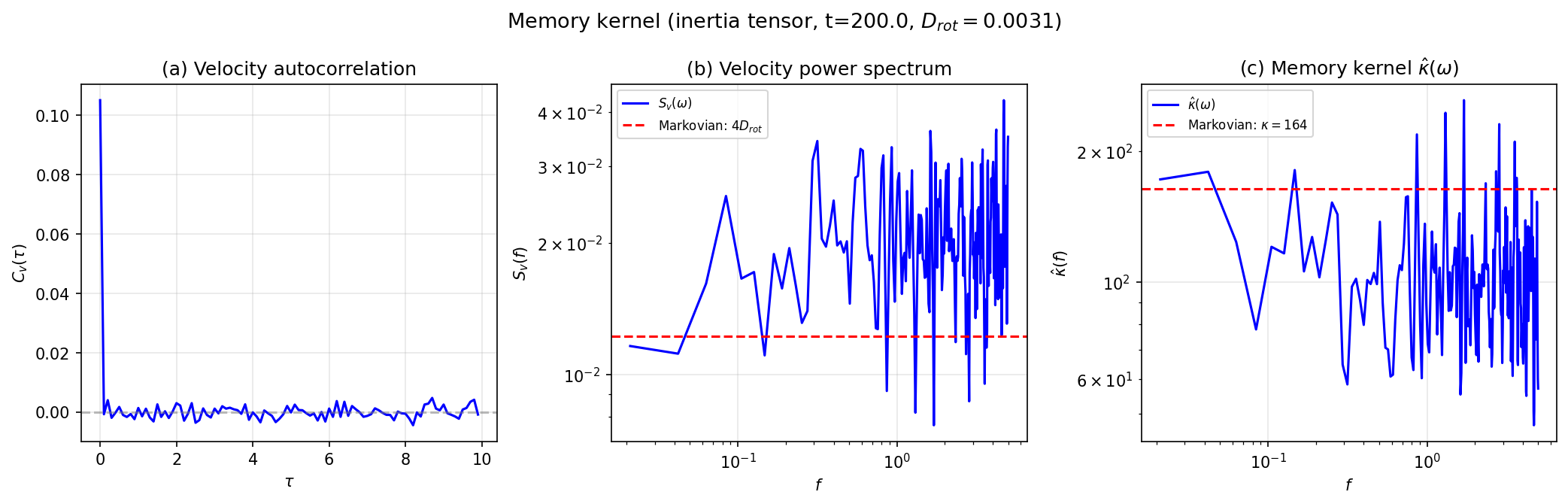
The result is clear: the orientation dynamics is Markovian when measured correctly with the inertia tensor. The velocity autocorrelation $C_{v}(\tau)$ decays to zero within one time step ( $C_{v}(\Delta t)/C_{v}(0)=-0.007\approx 0$ ), the velocity power spectrum is approximately flat (white noise), and $\hat{\kappa}(\omega)$ is constant. The inertia tensor method uses all $N$ particle positions to determine the ring plane, filtering out fast thermal noise and producing a clean measurement of the slow collective coordinate.

In the hierarchy of Section 4.4, the non-Markovian action (67) is the fundamental result of the BO reduction, and the Markovian action (68) is its $\kappa(\tau)\to\kappa\delta(\tau)$ limit. The data are consistent with the Markovian limit over the time resolution and frequency window accessible to the inertia-tensor estimator: no statistically significant memory-kernel structure is resolved in the present simulations. We do not infer global Markovianity from this; we infer that the Markovian $\mathbb{RP}^{2}$ NLSM is consistent with the orientation data within the bandwidth and statistics of the inertia-tensor measurement.

Density-density correlator from a 100-realization ensemble.

All diagnostics above use only the scalar orientation $\hat{\mathbf{n}}(t)$ extracted by the inertia tensor. A more stringent test of the $\mathbb{RP}^{2}$ NLSM is the full spatial density-density correlator

C_{\rho}(\gamma,\tau)=\left\langle\rho(x,t)\,\rho(x^{\prime},t+\tau)\right\rangle,

with $\gamma=\arccos(x\cdot x^{\prime})$ the great-circle angle between the two spatial arguments on $S^{2}$ . Its $\mathbb{RP}^{2}$ -NLSM prediction (76) depends on only two ingredients: the ring profile $f_{0}$ (through its Legendre coefficients $c_{\ell}$ ) and the orientation autocorrelation $q(\tau)=e^{-2D_{\text{rot}}\tau}$ . Both ingredients are measured directly from the same particle data, so the comparison is parameter-free once these two low-energy inputs are fixed from simulation: the test verifies that the $\mathbb{RP}^{2}$ -NLSM reduction propagates correctly into the density sector (a closure test), not that the F2 theory predicts $C_{\rho}$ from the microscopic action alone, which would require computing $f_{0}$ and $D_{\text{rot}}$ from first principles. In what follows we make the construction explicit.

Ensemble protocol. We ran $100$ independent particle simulations at $N=400$ , $T=0.4$ , $\sigma=1$ , each with an independent realization of the quenched couplings $\phi_{nm}$ and of the initial configuration, using $dt=0.0025$ , an equilibration time $t_{\text{eq}}=10$ , and a tracking time $t_{\text{track}}=40$ per realization, with snapshots recorded at $\Delta t_{\text{rec}}=0.25$ ( $160$ snapshots per realization). All $100$ runs formed rings.

Empirical $\langle C_{\rho}(\gamma,\tau)\rangle$ from the particle data. For each snapshot we reconstruct the smooth lab-frame density field $\rho(x,t)$ by Fisher-von Mises kernel density estimation (bandwidth $\sigma_{\text{KDE}}=0.1$ rad, normalized so that $\int_{S^{2}}\rho\,d\Omega=1$ ) on a uniform-area grid of $1800$ points, and expand it in real spherical harmonics up to $\ell_{\max}=30$ , $\rho(x,t)=\sum_{\ell m}a_{\ell m}(t)\,Y_{\ell m}(x)$ . Because the disorder-averaged ensemble is SO(3)-isotropic, the correlator reduces to its Legendre form

\langle C_{\rho}(\gamma,\tau)\rangle=\sum_{\ell=0}^{\ell_{\max}}\frac{2\ell+1}{4\pi}\,A_{\ell}(\tau)\,P_{\ell}(\cos\gamma),\qquad A_{\ell}(\tau)=\frac{1}{2\ell+1}\sum_{m}\overline{a_{\ell m}(t)\,a_{\ell m}(t+\tau)},

(82)

where the overline denotes the joint time-origin and disorder average over the $100$ runs. Equation (82) is what we plot as the empirical curves in Fig. 7(a,b); no SO(3) simulation is run at this stage.

Theoretical $C_{\rho}^{\mathrm{SO(3)}}(\gamma,\tau)$ . For the $\mathbb{RP}^{2}$ -NLSM prediction we do not run a separate $\mathbb{RP}^{2}$ -NLSM simulation and compute its density correlator empirically. Instead, we evaluate the closed-form expression for $\langle C_{\rho}(\gamma,\tau)\rangle$ that was derived analytically from the $\mathbb{RP}^{2}$ NLSM in Section 4.5 (the reduction formula (76)),

C_{\rho}^{\mathrm{SO(3)}}(\gamma,\tau)=\sum_{\ell=0}^{\ell_{\max}}\frac{c_{\ell}^{\,2}}{2\ell+1}\,e^{-\ell(\ell+1)\,D_{\text{rot}}\,|\tau|}\,P_{\ell}(\cos\gamma),

(83)

directly on the same $(\gamma,\tau)$ grid as the empirical estimator (82). The theoretical content entering Fig. 7 is therefore the functional form of (83): given $\{c_{\ell},D_{\text{rot}}\}$ , the formula fully determines the shape of $C_{\rho}^{\mathrm{SO(3)}}(\gamma,\tau)$ in both $\gamma$ and $\tau$ . An alternative route (simulating the $\mathbb{RP}^{2}$ -NLSM SDE (79) and dressing each sampled $\hat{\mathbf{n}}(t)$ with the ring profile $\rho(x,t)=f_{0}(\hat{\mathbf{n}}(t)\cdot\mathbf{x})$ before computing the density correlator via the same KDE/SH pipeline) yields the same answer up to Monte Carlo noise, since (83) is exactly the prediction of that procedure.

The two inputs $\{c_{\ell},\,D_{\text{rot}}\}$ of (83) are measured directly from the particle data of the same $100$ -realization ensemble (not fit to Fig. 7). Specifically: (i) the Legendre coefficients $c_{\ell}=\tfrac{2\ell+1}{2}\int_{-1}^{1}f_{0}(u)\,P_{\ell}(u)\,du$ come from the histogram of the ring-frame coordinate $u=\hat{\mathbf{n}}(t)\cdot\mathbf{x}_{n}(t)$ pooled over all $100\times 160\times 400$ particle-snapshot samples, which gives a dense estimate of the stationary (in the ring frame) profile $f_{0}$ ; (ii) the rotational diffusion coefficient $D_{\text{rot}}$ is the log-slope fit of the pooled orientation autocorrelation $\langle q(\tau)\rangle_{\text{disorder}}$ , and yields the value $D_{\text{rot}}=0.0035$ shown in Fig. 7(c). The comparison between (82) and (83) in Fig. 7(a,b) is therefore a parameter-free test of the functional form predicted by the $\mathbb{RP}^{2}$ -NLSM effective theory: once $f_{0}$ and $D_{\text{rot}}$ are fixed from two independent orientation-sector diagnostics (the ring profile and the orientation autocorrelation), the full spatial $(\gamma,\tau)$ dependence of $\langle C_{\rho}\rangle$ is predicted by (83) with no additional fit parameters.

The pooled fit yields $D_{\text{rot}}=0.0035$ , consistent with the ensemble mean of Table 1 ( $\langle D_{\text{rot}}\rangle=0.003\pm 0.002$ ) and with the single long run ( $0.0031$ ), but now disorder-averaged with an order-of-magnitude more statistics than the earlier $10$ -realization ensemble. The on-ring decay slices of panel (b) agree with the $\mathbb{RP}^{2}$ -NLSM prediction at the few-percent level over the full accessible range of $\tau$ ; the small residual at the $\gamma\to 0,\pi$ peaks of the static correlator (panel a) is a finite-bandwidth artifact of the KDE (FWHM $\approx 5.7^{\circ}$ ) combined with the finite resolution of the pooled profile $f_{0}$ measured from the ring-frame histogram. Crucially, the density sector is reproduced without any free parameters beyond those already fixed by the orientation-sector diagnostics: the same $f_{0}$ and $D_{\text{rot}}$ that describe the scalar collective coordinate also determine the full spatial density dynamics, confirming the SO(3) effective theory at this stronger level.

Why the agreement is non-trivial. The closed-form prediction (83) was derived in Section 4.5 under the rigid-ring ansatz $\rho(x,t)=f_{0}(\hat{\mathbf{n}}(t)\cdot\mathbf{x})$ , in which the static profile $f_{0}$ is passively advected by the stochastic orientation $\hat{\mathbf{n}}(t)$ . The particle simulation does not satisfy this ansatz exactly: $400$ particles produce finite- $N$ shot noise at every snapshot, the ring has internal (breathing, azimuthal) fluctuations of the gapped $\delta\rho$ modes, and disorder heterogeneity across realizations gives a per-sample spread in $D_{\text{rot}}$ of roughly a factor of two (Table 1). Any of these effects could have contaminated $C_{\rho}$ at the level of the signal, and each one failing separately would have produced a distinct diagnostic signature. The agreement in Fig. 7 therefore tests four things simultaneously. First, the Born-Oppenheimer decoupling of the gapped $\delta\rho$ modes from the slow orientation, which is the premise of the collective-coordinate reduction of Section 4: if $\epsilon=D_{\text{rot}}/m^{2}_{\text{gap}}$ were not small, the $\ell$ -th Legendre mode would acquire additional decay channels and the single exponential $e^{-\ell(\ell+1)D_{\text{rot}}\tau}$ would break. Second, the full Fokker-Planck spectrum $\lambda_{\ell}=\ell(\ell+1)D_{\text{rot}}$ of free diffusion on $S^{2}$ : the measurement of $D_{\text{rot}}$ at $\ell=1$ (through $q(\tau)$ ) is extrapolated to all $\ell\leq\ell_{\max}=30$ by the formula, and the off-center $\gamma$ slices of Fig. 7(b) sample different combinations of these modes, providing an independent check of the higher- $\ell$ rates. Third, suppression of the finite- $N$ shot noise at the few percent level in the pooled correlator, which would otherwise appear as a $\tau$ -independent offset at large lags. Fourth, the commutativity of the quenched disorder average with the $\mathbb{RP}^{2}$ -NLSM reduction at $N=400$ : a single pooled $D_{\text{rot}}=0.0035$ describes the full $(\gamma,\tau)$ dependence, so the sample-to-sample heterogeneity in $D_{\text{rot}}$ does not distort the functional form of $\langle C_{\rho}\rangle$ . The structure of the test is the same as a chiral-Lagrangian consistency check in QCD, in which $f_{\pi}$ measured from one observable (pion decay) is required to reproduce a qualitatively different observable (e.g. $\pi\pi$ -scattering) without further fitting; here $f_{0}$ and $D_{\text{rot}}$ measured from the orientation sector reproduce the full density-sector correlator (83) through an exponent chain $\ell(\ell+1)$ that is not present in the input.

Overall consistency assessment.

After $D_{\text{rot}}$ is fixed from the particle simulation (Tier 2 of the three-tier framework, Section 4.7), the Markovian $\mathbb{RP}^{2}$ NLSM model (68) reproduces the tested observables of the orientation dynamics, within numerical resolution: (i) exponential autocorrelation $C(\tau)=e^{-2D_{\text{rot}}\tau}$ (Fig. 5, panel d); (ii) MSD $=2(1-e^{-2D_{\text{rot}}\tau})$ (panel e); (iii) Markovian power spectrum $\omega^{-2}$ (panel f); (iv) isotropic exploration of $S^{2}$ with no preferred direction (panels a–c, the three components $n_{x},n_{y},n_{z}$ all showing similar diffusive volatility); (v) zero deterministic drift, confirmed by the azimuthal velocity distribution $|\text{mean}/\text{std}|=10^{-4}$ (Fig. 4, panel b); (vi) Markovian velocity (white noise, $C_{v}(\Delta t)/C_{v}(0)\approx 0$ ; Fig. 6, panel a); (vii) constant memory kernel $\hat{\kappa}(\omega)\approx\kappa$ (Fig. 6, panel c); and (viii) the disorder-averaged density-density correlator $\langle C_{\rho}(\gamma,\tau)\rangle$ from a 100-realization ensemble (Fig. 7), which agrees with the parameter-free SO(3) prediction (76) at the few-percent level over the full $(\gamma,\tau)$ domain. The single parameter $D_{\text{rot}}$ (equivalently $\kappa=1/(2D_{\text{rot}})$ ), measured from one observable (e.g., the autocorrelation decay rate), predicts all others with no free parameters.

This realizes in concrete form the Tier-2 strategy of Section 4.7: the form of the action is fixed by the SO(3) $\to$ SO(2) symmetry breaking, and the single low-energy constant $D_{\text{rot}}$ , measured from one observable, controls all others. The QCD/ $f_{\pi}$ analogy and the open Tier-3 computation are discussed there. The measured $N$ -scaling $D_{\text{rot}}\sim N^{-1.7}$ (Table 2, Fig. 3) is steeper than the mean-field $1/N$ and remains to be explained at the microscopic level.

5.3 Universality: what interaction potentials produce rings on $S^{2}$

The $\mathbb{RP}^{2}$ -NLSM effective theory was derived from the F2 model on $S^{2}$ with the linear geodesic-distance potential $U_{ij}=\phi_{ij}\,d(x_{i},x_{j})$ . To test whether the ring formation and the resulting $\mathbb{RP}^{2}$ -NLSM dynamics are specific to this potential or reflect a more general phenomenon, we simulated systems with logarithmic potentials on $S^{2}$ .

Soft Coulomb model.

We consider the potential $U_{ij}=\phi_{ij}\,\log(d_{\text{geo}}(x_{i},x_{j})+d_{\min})$ , where $d_{\text{geo}}$ is the geodesic distance, $\phi_{ij}=\pm 1$ (discrete random couplings), and $d_{\min}$ is a soft regularization parameter. The force is $1/(d_{\text{geo}}+d_{\min})$ , with ratio $F_{\max}/F_{\min}=(d_{\max}+d_{\min})/d_{\min}$ (where $d_{\max}=\pi$ on $S^{2}$ ). For $d_{\min}\to 0$ , the force is strongly distance-dependent (short-range dominated), and no ring formation is observed. For larger $d_{\min}$ , the force becomes more uniform, approaching the constant-force regime of the F2 model.

Three-model comparison.

Figure 8 compares three models at $N=400$ , $t=200$ , all analyzed with the inertia tensor method:

Model	$T$	Force ratio	Ring	FWHM	$D_{\text{rot}}$
F2 (linear)	0.4	1:1	YES	$11^{\circ}$	0.0031
Soft Coulomb, $d_{\min}\!=\!3$	0.2	2:1	YES	$13^{\circ}$	0.0011
Soft Coulomb, $d_{\min}\!=\!1$	0.2	4.1:1	YES	$9^{\circ}$	0.0009

Table 3: Comparison of three potential types with long-run inertia tensor analysis (

N=400

t=200

). The two soft Coulomb runs use

T=0.2

rather than

T=0.4

, so absolute values of

D_{\text{rot}}

are not directly comparable across rows; the qualitative point is that all three potentials form rings and exhibit Markovian

\mathbb{RP}^{2}

diffusion.

All three models form rings and exhibit the same SO(3) diffusion dynamics: exponential autocorrelation, MSD saturating at $2$ , and Markovian $\omega^{-2}$ power spectrum. The $d_{\min}=1.0$ case produces the tightest ring (FWHM $=9^{\circ}$ , anisotropy ratio $50$ ) and the slowest diffusion ( $\tau_{c}=562$ ), despite having the largest force ratio ( $4.1$ : $1$ ). Ring formation therefore persists across a range of force profiles within the soft-kernel family, not just the constant-force (F2) limit; a kernel-family-dependent reading of the universality criterion is given in the “Universality of the SO(3) reduction” paragraph below.

Truncated geodesic-log potential.

A fourth model uses the geodesic-distance logarithmic potential with a hard floor: $V=\max(U_{\min},\,\log(d_{\text{geo}}))$ , where $U_{\min}$ is a tunable parameter. The force is $1/d_{\text{geo}}$ for $d_{\text{geo}}>e^{U_{\min}}$ and zero for $d_{\text{geo}}<e^{U_{\min}}$ (flat bottom). This model has the exact $1/d$ Coulomb force at all distances beyond the cutoff $e^{U_{\min}}$ .

Ring formation does not occur for $U_{\min}\geq 0$ (cutoff $\geq 1$ , force ratio $\lesssim 3$ : $1$ ), despite the force ratio being comparable to the successful soft Coulomb cases. Ring formation is observed for $U_{\min}=-2.15$ (cutoff $\approx 0.12$ , force ratio $\approx 27$ : $1$ ), but the resulting ring is much broader (FWHM $=24^{\circ}$ , anisotropy ratio $3.7$ ) than the soft Coulomb or F2 rings ( $10$ – $12^{\circ}$ ). The difference is that the hard-floor truncation creates a zero-force region ( $d<e^{U_{\min}}$ ) where nearby particles can cluster without any restoring force, partially disrupting the collective ring ordering. The soft Coulomb model $\log(d+d_{\min})$ avoids this by maintaining a nonzero (though reduced) force at all distances.

Model	Force ratio	FWHM	Frac. eq.	Ring
F2 (linear)	1:1	$11^{\circ}$	1.00	YES
Soft Coulomb $d_{\min}\!=\!1$	4.1:1	$10^{\circ}$	0.98	YES
Soft Coulomb $d_{\min}\!=\!3$	2.0:1	$12^{\circ}$	0.99	YES
Trunc log $U_{\min}\!=\!{-}2.15$	27:1	$24^{\circ}$	0.91	YES
Trunc log $U_{\min}\!=\!0$	3.1:1	—	—	NO
Chord Coulomb (2D), $\log c$	$\infty$	—	—	NO
Chord Coulomb (3D), $1/c$	$\infty$	—	—	NO

Table 4: Ring formation across all seven potential types tested (

N=400

T=0.2

–

0.4

, discrete

\pm 1

couplings except F2 which uses Gaussian). The column “Frac. eq.” is the fraction of particles within the fitted ring band (Gaussian within

\pm 2\sigma

of the ring centre). Ring formation requires a force that remains effective across the full sphere; both vanishing antipodal force (chord Coulombs, whether 2D

\log c

or 3D

1/c

) and hard-floor truncation at moderate cutoff (truncated log,

U_{\min}\geq 0

) prevent it.

Chord-distance Coulomb and the role of geometry.

The exact 2D Coulomb potential on $S^{2}$ (the Green’s function of the Laplace-Beltrami operator) is $V(\theta)=-(1/2\pi)\log(2\sin(\theta/2))$ , where the argument is the chord distance $c=2\sin(\theta/2)=|\mathbf{x}_{i}-\mathbf{x}_{j}|$ (the 3D Euclidean distance between two points on the unit sphere), as discussed by Caillol [41] and by Forrester, Jancovici, and Madore [42]. This is distinct from $\log(d_{\text{geo}})$ , where $d_{\text{geo}}=R\theta$ is the geodesic distance (equal to $\theta$ on the unit sphere $R=1$ ). The chord distance arises from the intrinsic geometry of $S^{2}$ through the Laplace-Beltrami operator, regardless of whether the electric field propagates through the interior or along the surface.

The force (per unit coupling) for the chord-distance potential is $F(s)=-dV/ds$ , which on the unit sphere gives $F=\cot(s/2)/2$ (where $s=d_{\text{geo}}$ is the geodesic distance). This force vanishes at the antipodal point ( $s=\pi$ ): particles on opposite sides of the sphere do not interact. This makes the chord-distance Coulomb potential effectively short-ranged on $S^{2}$ , and simulations confirm that it does not produce ring formation. The soft Coulomb model $\log(d_{\text{geo}}+d_{\min})$ avoids this problem because its force $1/(d_{\text{geo}}+d_{\min})$ remains nonzero at all distances, including the antipodal point.

3D Coulomb on the sphere.

The same antipodal-vanishing obstruction also rules out the ordinary three-dimensional Coulomb interaction $V(c)=1/c$ for particles constrained to $S^{2}$ , with $c$ the embedding chord distance. The tangent-plane component of the 3D Coulomb force between two surface points is $|F_{\perp}(s)|=\cos(s/2)/(4\sin^{2}(s/2))$ , which has the same $\cos(s/2)$ factor as the 2D chord-log potential and therefore vanishes at the antipodal point $s=\pi$ . Simulations using this potential with a hard-core cutoff $c>2r_{p}$ confirm that no ring forms, consistent with the general criterion: it is the vanishing of the force at the cut locus, not the specific functional form of the potential, that breaks the ring-forming mechanism. Both the 2D chord Coulomb ( $\log c$ , the Green’s function of the Laplace-Beltrami operator) and the 3D chord Coulomb ( $1/c$ , the interaction mediated by the embedding $\mathbb{R}^{3}$ ) therefore fall into the same “effectively short-ranged on $S^{2}$ ” class.

Universality of the $\mathbb{RP}^{2}$ -NLSM reduction.

The scan suggests an empirical criterion for ring formation: the interaction should remain effective at antipodal-scale separations on $S^{2}$ . The features common to the ring-forming runs are: (i) particles confined to $S^{2}$ ; (ii) quenched random pairwise couplings; (iii) an interaction whose force does not vanish at the cut locus of the manifold. A naive global force-ratio threshold is insufficient as a single number across kernel families. Within the soft-kernel family (F2 with $V=d$ , soft Coulomb with various $d_{\min}$ ), the ring-forming runs sit at force ratios up to $4.1$ : $1$ in the present scan; a hard-floor truncated logarithm can still form a (broader) ring at much larger nominal force ratio ( $\approx 27$ : $1$ ), because the hard-floor cutoff changes the near-field clustering dynamics and so changes which configurations are stable. We therefore treat the force-ratio threshold as kernel-family dependent: within a smooth kernel family it provides a useful empirical indicator (with order $\sim 5$ : $1$ separating the present soft-kernel ring-forming and non-forming cases), but it does not transfer across families. Both chord Coulombs (the 2D $\log c$ and the 3D $1/c$ , $F_{\max}/F_{\min}\to\infty$ ) and the unregularized geodesic Coulomb ( $F_{\max}/F_{\min}\to\infty$ ) violate the cut-locus criterion and show no ring formation. We state these observations as numerical conjectures: an analytic stability analysis of the uniform state and of the ring saddle under general kernels, which would turn the empirical indicators into derived selection rules, is left to future work. Within the ring-forming subclass tested, the form of the effective low-energy theory appears universal; only $D_{\text{rot}}$ (the analog of $f_{\pi}$ ) is model-dependent.

6 Discussion and Future Directions

We now turn to physical realizations of the F2 ring, connections to other areas of physics, and open questions.

6.1 Physical Realizations

Three ingredients are needed to realize the F2 ring on a physical platform: (i) a closed 2D surface (or thin shell) on which the constituent objects (particles, atoms, or electrons) are confined; (ii) quenched random pairwise couplings between them; and (iii) a pairwise force whose magnitude remains nonzero across the full diameter of the surface (Section 5.3). We sketch three classes of candidates, grouped by whether the underlying dynamics is classical stochastic or genuinely quantum.

Classical platform: charged colloids on a soft membrane.

A spherical polymer vesicle of radius $R\sim 1$ – $10\;\mu$ m, decorated with two species of charged colloidal nanoparticles ( $r\sim 10$ – $100\;$ nm, charges $q=\pm 1$ ), realizes the microscopic F2 model directly at the level of classical stochastic dynamics. For $r\sim 50\;$ nm on $R\sim 1\;\mu$ m, the dimensionless contact distance $2r/R\approx 0.1$ places the truncated-log potential of Section 5.3 at $U_{\min}\approx-2.3$ , inside the ring-forming regime. The ring orientation $\hat{\mathbf{n}}(t)$ can be tracked by fluorescence microscopy, and $D_{\text{rot}}$ extracted from the orientation autocorrelation $q(\tau)$ .

The main experimental constraint is the range of the effective surface interaction: the bare 2D Coulomb on $S^{2}$ is effectively short-ranged in our sense (its force vanishes at the antipodal point; Section 5.3), so the pair potential must be engineered. Three mechanisms can produce a force that stays effective across the sphere. (i) Membrane-mediated fluctuation interactions. Inclusions that deform or stiffen the membrane couple through its thermal height fluctuations; the resulting interaction decays only algebraically with geodesic distance and, on a sphere whose bending rigidity is not much larger than $k_{B}T$ , is long-ranged in our sense. (ii) Thick-shell electrostatics. For a spherical conducting shell of thickness $h$ , the surface-to-surface potential interpolates between the chord form $\log c$ (for $h\ll R$ , the thin-shell Laplace-Beltrami Green’s function) and a geodesic form (for $h\gg R$ , where the field is expelled from the interior), with the force ratio $F_{\max}/F_{\min}$ tunable by $h/R$ and the dielectric contrast. (iii) Screened bulk electrostatics combined with surface binding. Screening the 3D Coulomb field (by embedding the vesicle in a high-permittivity or ionic solvent) suppresses through-bulk interactions so the effective coupling is controlled by surface terms whose profile can be tuned via the joint screening length and shell thickness. In each case the effective pair potential is a physically distinct interaction, not a regularization of the bare Laplace-Beltrami Coulomb; the criterion of Section 5.3 then selects which implementations form rings.

Quantum platforms.

A genuine quantum realization replaces Brownian particles by atoms, ions, or electrons constrained to a 2D shell. Three concrete directions are:

•

Cold atoms on a shell trap. Optically trapped or ”bubble-trapped” Bose gases can be confined to thin spherical shells. Spatial random potentials (laser speckle, optical disorder) and tunable contact interactions (Feshbach resonances) could produce a quantum analog of the F2 model; the orientation $\hat{\mathbf{n}}(t)$ of the resulting ring condensate would be a genuine quantum coordinate.
•

Electronic shells. The $\pi$ -electron systems of fullerenes, carbon nanoshells, or thin films of 3D topological insulators shaped into closed surfaces carry electronic degrees of freedom confined to an approximately 2D curved geometry. Random dopants or chemisorbed impurities provide the quenched couplings; the screened electron-electron interaction projected onto the shell supplies the long-range pair force.
•

Skyrmion-like textures on curved magnetic surfaces. Magnetic thin films deposited on spherical or ellipsoidal substrates, with engineered random exchange couplings (frustrated magnetism), could carry a ring-like magnetization texture whose orientation is a quantum collective coordinate.

In all three quantum platforms, the $\mathbb{RP}^{2}$ NLSM of Section 4 emerges as the low-energy Hamiltonian of the orientation sector, not merely as the Euclidean action of a classical stochastic process. The rotational diffusion coefficient $D_{\text{rot}}$ is replaced by a genuine kinetic coefficient $\hbar^{2}/(2\mathcal{I})$ with $\mathcal{I}$ an effective moment of inertia, and the combinations $\ell(\ell+1)D_{\text{rot}}$ are true energy levels of the orientation rather than Fokker-Planck relaxation rates.

6.2 Connections to Other Physics Phenomena

Classical relaxation vs. quantum energy spectrum.

In the classical stochastic realization studied here, the orientation dynamics is a Fokker-Planck diffusion on $\mathbb{RP}^{2}$ (lifted to $S^{2}$ ), and $\lambda_{\ell}=\ell(\ell+1)\,D_{\text{rot}}$ is the relaxation rate of the $Y_{\ell m}$ component of the orientation distribution, not an energy. A genuine quantum implementation would replace the Fokker-Planck operator by the rotor Hamiltonian $\mathbf{L}^{2}/(2\mathcal{I})$ , with energy levels $E_{\ell}=\ell(\ell+1)\,\hbar^{2}/(2\mathcal{I})$ and $\mathcal{I}$ a platform-dependent moment of inertia. The two formulae have the same $\ell(\ell+1)$ dependence on representation but encode different physical content; we use the quantum analogy below only to motivate experimental directions, never to claim that a relaxation rate is an energy.

Quantum-realization outlook: nematic-type ring-orientation qubit on $\mathbb{RP}^{2}$ .

Because the physical orientation manifold is $\mathbb{RP}^{2}=S^{2}/\mathbb{Z}_{2}$ (Section 4.1), the single-valued quantum Hilbert space of the orientation sector is the even- $\ell$ subspace of $L^{2}(S^{2})$ , spanned by spherical harmonics with $\ell=0,2,4,\ldots$ . The lowest two levels are the $\ell=0$ singlet and the $\ell=2$ quintuplet, separated by the rotor gap $\Delta_{02}=E_{2}-E_{0}=6\,\hbar^{2}/(2\mathcal{I})=3\hbar^{2}/\mathcal{I}$ in a quantum implementation along the lines of Section 6.1. The $\ell=1$ triplet is odd under $\hat{\mathbf{n}}\to-\hat{\mathbf{n}}$ and is excluded from the physical sector on $\mathbb{RP}^{2}$ (it can be reached only by the $\theta=\pi$ quantization sector of Section 4.1, “Topological aspects of the $\mathbb{RP}^{2}$ target”, a spin-1/2-like sector that we do not consider here).

The natural qubit on $\mathbb{RP}^{2}$ is therefore a nematic-type two-level system built from the $\ell=0$ singlet and one component of the $\ell=2$ quintuplet isolated by a quadrupolar (tensor) symmetry-breaking field. A traceless symmetric coupling $H_{ij}\,n^{i}n^{j}$ , which is $\mathbb{Z}_{2}$ -invariant in $\hat{\mathbf{n}}$ and therefore admissible on $\mathbb{RP}^{2}$ , splits the $\ell=2$ quintuplet (axial vs. planar anisotropy) and selects a logical pair with energy gap of order $\Delta_{02}$ shifted by the quadrupolar splitting. A scalar Zeeman-like coupling $\vec{h}\cdot\hat{\mathbf{n}}$ is forbidden on $\mathbb{RP}^{2}$ (it is parity-odd in $\hat{\mathbf{n}}$ and therefore couples only across the trivial / non-trivial $\mathbb{Z}_{2}$ -sectors); the appropriate experimental probes are quadrupolar / strain / dielectric-anisotropy fields, exactly the setup that drives nematic-liquid-crystal director dynamics. The spectral gap $m^{2}_{\text{gap}}$ to internal ring excitations (Section 4.3) protects the orientation sector against leakage to bulk modes in the same way as in the skyrmion-helicity qubit of Psaroudaki and Panagopoulos [34]; we refer the reader to that work for the analogous analysis in the magnetic-skyrmion context, with the caveat that the $\mathrm{U}(1)$ helicity coordinate of a magnetic skyrmion is replaced here by the projective director on $\mathbb{RP}^{2}$ and the natural coupling family changes from Zeeman-like to quadrupolar accordingly. Calibrating the classical (Fokker-Planck) tensor response of the orientation on a colloidal platform before a quantum implementation is the natural experimental sequence.

Adiabatic rotational reductions vs. true symmetry breaking.

The F2 reduction from a microscopic field theory to an effective $\mathrm{SO}(3)$ classical-stochastic theory for a slow orientation has direct physical precedent in adiabatic-rotation problems: the Bohr-Mottelson picture of nuclear rotational bands [29], where a deformed nucleus breaks rotational symmetry in the body frame and the slow lab-frame orientation produces the spectrum $E_{\ell}=\ell(\ell+1)\hbar^{2}/(2\mathcal{I})$ , and the Born-Oppenheimer treatment of molecular rotation [30, 31], where fast electronic and vibrational modes are integrated out to yield the same $\ell(\ell+1)$ ladder. The F2 ring is the classical-stochastic counterpart: the moment of inertia plays the role of the stiffness $\kappa$ , and the rotational quanta $\hbar^{2}/(2\mathcal{I})$ are replaced by the relaxation rates $\ell(\ell+1)D_{\text{rot}}$ of the spherical harmonics. The kinematic action $\propto\int|\dot{\hat{\mathbf{n}}}|^{2}\,dt$ also coincides with that of the Haldane $\mathrm{O}(3)$ NLSM [26, 27] and the Frank elastic theory of nematic liquid crystals [35], but with a conceptual distinction: in those systems rotational symmetry is spontaneously broken in the thermodynamic limit and the slow modes are genuine Nambu-Goldstone modes (continuous gapless spectrum), whereas in the F2 model the orientation is broken only adiabatically and is restored by the rotational diffusion of $\hat{\mathbf{n}}(t)$ . The slow F2 mode is not a Goldstone in the strict sense but a discrete pair of soliton zero modes (in the sense of Rajaraman [22], Sec. 5.5) promoted to a collective orientation coordinate, overdamped (type-A) rather than propagating (type-B, as in the symplectic Hamiltonian cases above).

Mean-field glasses and SYK-type dynamics.

The disorder-averaged action of Section 3, with its non-local temporal kernel and time-reparametrization quasi-invariance, shares its formal structure with the dynamics of spherical $p$ -spin models and SYK-type systems [4, 5]. The analogy is not merely formal: in the glassy regime the density two-point function is expected to exhibit aging and a nontrivial Parisi-type structure, and the mapping between classical Langevin dynamics and quantum Hamiltonians established by Facoetti et al. [5] suggests that the F2 density sector may inherit the same SYK-like correlation structure. The geometric setting, a physical 2D surface embedded in 3D space rather than an abstract hypersphere in spin space, raises the prospect of probing these phenomena in a system where the order parameter is directly observable.

Non-perturbative field theory and adiabatic dimension reduction.

Ring formation is itself a non-perturbative effect: the density profile $f_{0}(\hat{\mathbf{n}}\cdot\mathbf{x})$ is a saddle point that cannot be reached by any finite-order expansion around the uniform state. We refer to the emergence of such configurations as adiabatic dimension reduction: at any instant the density concentrates on a lower-dimensional submanifold of the background (a great circle on $S^{2}$ , a pair of small circles on $T^{2}$ ) with a definite orientation, while that orientation itself performs a slow stochastic motion, so that the long-time-averaged state restores the rotational invariance of the underlying manifold. The slowly moving collective excitations seen in the FBP particle model and reproduced by the F2 field theory, rings on $S^{2}$ and pairs of rings on $T^{2}$ whose centers drift coherently while the internal density supports finite-frequency breathing and azimuthal fluctuations, are reminiscent of the breather solutions of relativistic and integrable field theories, in which a localized non-perturbative profile carries a slow collective coordinate alongside oscillatory internal modes (Rajaraman [22], Ch. 2). In this respect the F2 model provides a tractable laboratory for studying adiabatic dimension reduction, instanton-like transitions between orientations, and the coupling of the collective coordinate to its gapped fluctuations through the Faddeev-Popov sector of Section 4.2.

6.3 Open Questions

Several questions remain open beyond the universal SO(3) description. Does the disorder-averaged field theory exhibit replica symmetry breaking in the density sector, and if so, what is the structure of the Parisi order parameter in this geometric setting? What is the phase diagram in the $(T,J,\lambda)$ parameter space, and at what control-parameter values do phase transitions between uniform and ring states occur? Beyond the mean-field treatment developed here, how do fluctuations affect the formation of the dimension-reduced structure, and what is the nucleation barrier for creating a ring? Beyond these conceptual questions, the technical program of computing $D_{\text{rot}}$ from the microscopic theory and extending the construction to other geometries and to a dynamical metric defines the next stage of this work.

7 Summary

We set out to determine the statistical field theory that governs the thermodynamic limit of frustrated Brownian particles on a two-dimensional Riemannian manifold and to extract its universal low-energy content. The main achievements of the paper are the following.

(1) The F2 statistical field theory.

Starting from the $N$ -body overdamped Langevin dynamics of Ref. [1], the large- $N$ limit yields a covariant statistical field theory for a smooth density field $\rho(x,t)$ , which we call the F2 model. Cast as an MSRJD path integral and averaged over quenched disorder, the theory produces a single-field effective action with local and non-local (in space and time) self-interactions characteristic of spin-glass dynamics.

(2) The effective Dean-Kawasaki equation of the F2 model.

Saddle-point analysis of the F2 generating functional produces the covariant effective Dean-Kawasaki equation of Section 3.6: a nonlinear functional Langevin equation for the smooth density field $\rho(x,t)$ , in which the bare local Dean-Kawasaki noise is dressed into a self-consistent two-time kernel inherited from the disorder average. This is distinct from the exact Dean-Kawasaki SPDE for the singular empirical density, which enters only as an intermediate step in the construction. The mean-field reduction of the effective equation governs the evolution of $\langle\rho(x,t)\rangle$ on the background manifold and is the field-theoretic counterpart of the Cugliandolo-Kurchan equations of mean-field glass theory, adapted to a conserved density on a curved surface.

(3) The $\mathbb{RP}^{2}$ nonlinear sigma model in (0+1) dimensions.

Combining the symmetry analysis of the F2 action with the ring-formation pattern observed in the particle simulations of Ref. [1], we carried out a low-energy reduction. The $\mathrm{SO}(3)\to\mathrm{SO}(2)$ symmetry breaking singles out the ring orientation as the slow degree of freedom, and integrating out the gapped density fluctuations by the Gervais-Jevicki-Sakita collective-coordinate construction with Faddeev-Popov gauge fixing yields the nonlinear sigma model (NLSM) on the real projective plane $S^{2}/\mathbb{Z}_{2}=\mathbb{RP}^{2}$ (the $\mathbb{RP}^{2}$ NLSM on the projective rotor space) in (0+1) dimensions; the orientation is a director, since $\hat{\mathbf{n}}$ and $-\hat{\mathbf{n}}$ describe the same density of the even-profile ring. The model is governed by a single low-energy constant $D_{\text{rot}}$ , with no potential and no Berry phase. A simulation of the $\mathbb{RP}^{2}$ NLSM with $D_{\text{rot}}$ fitted from a single observable reproduces the tested orientation- and density-sector diagnostics within numerical resolution after fixing $D_{\text{rot}}$ and, where needed, $f_{0}$ .

(4) Universality of ring formation and of the $\mathbb{RP}^{2}$ -NLSM dynamics.

On $S^{2}$ , the same ring geometry and the same $\mathbb{RP}^{2}$ -NLSM effective dynamics arise from a broader class of pairwise potentials than the linear geodesic form $V(d)=d$ of the original F2 model. Soft Coulomb potentials $V(d)=\log(d+d_{\min})$ at several values of $d_{\min}$ and the truncated geodesic-logarithm $V(d)=\max(U_{\min},\log d)$ in its ring-forming regime all produce rings that undergo $\mathbb{RP}^{2}$ -NLSM orientation dynamics indistinguishable from the F2 model in their scalar diagnostics (Section 5.3). What these tests select is a pairwise force that remains nonzero across the full diameter of $S^{2}$ . Both genuine Coulomb-type potentials on the sphere, namely the intrinsic 2D chord-logarithm $V(d)=\log(2\sin(d/2))$ (the Green’s function of the Laplace-Beltrami operator) and the restriction of the ordinary 3D Coulomb $V=1/|\mathbf{x}_{i}-\mathbf{x}_{j}|$ to the surface, fail this criterion: their forces vanish at the antipodal point, where all geodesics from a source refocus, and neither produces ring formation in our simulations.

The effective low-energy theory is insensitive to the microscopic form of the pairwise potential within the ring-forming subclass; only $D_{\text{rot}}$ is model-dependent. We therefore conjecture, and provide numerical evidence for, a universality class on $S^{2}$ whose defining feature is not any specific functional form of the potential but a pairwise force that remains effective across the cut locus of the sphere. Whether the same mechanism selects ring-forming potentials on two-dimensional manifolds of lower symmetry (torus, cylinder, smoothly deformed spheres) is a natural extension that is left for future work.

Future directions.

The framework developed here admits several natural extensions. The collective-coordinate construction should be repeated on the other fixed manifolds treated in the companion particle-simulation study [1], including the torus, the cylinder, and smoothly deformed spheres. On these manifolds the orientation target space and the selection rules that enforce the zero-torque and zero-Berry-phase properties on $S^{2}$ both change, so the exercise should separate what is specific to the sphere from what is truly geometry-independent.

Spatially extended versions of the F2 sigma model, in which the orientation field varies over a 2D domain (e.g., a soft membrane that supports multiple ring-forming patches, or multi-ring configurations on the torus), would activate the topological-defect content of the $\mathbb{RP}^{2}$ NLSM laid out in Section 4.1: half-integer disclinations of the director field from $\pi_{1}$ and hedgehog charges from $\pi_{2}$ , with the $\mathbb{Z}_{2}$ self-annihilation rule familiar from the nematic-defect literature [45, 46]. These spatially-textured extensions are the most direct route to making the $\mathbb{RP}^{2}$ topology of the orientation manifold experimentally observable beyond the selection-rule level resolved by the present (0+1)D analysis.

A second topological extension in a different direction is to add quantum spin-1/2 internal degrees of freedom to the FBP particles, with body-frame coupling to the ring orientation through a spin-orbit term. A $\hat{\mathbf{n}}\to-\hat{\mathbf{n}}$ flip is then a $\pi$ -rotation of the body frame and produces a $(-1)^{N_{s}}$ Berry phase from the $N_{s}$ body-frame-coupled spinors; for odd $N_{s}$ this realizes the $\theta=\pi$ (spinor) sector of the $\mathbb{RP}^{2}$ NLSM, inaccessible in the present spinless construction. The mechanism is the rotor analog of the Haldane $\theta$ -term distinction between integer-spin and half-integer-spin antiferromagnets, and connects to the skyrmion-qubit construction of Ref. [34] with the helicity coordinate replaced by the projective ring orientation.

Computing $D_{\text{rot}}$ from first principles through the self-consistency loop of Section 4.7 remains open and is the natural next step toward an ab initio prediction of the single low-energy constant that controls the effective theory. The non-Markovian regime, in which the memory kernel $\kappa(\tau)$ acquires nontrivial time structure, is the regime where the connection between the F2 model and glassy/SYK-type dynamics should become quantitatively testable, with the ring orientation providing a geometrically well-defined order parameter for aging measurements.

Finally, an experimental realization of the ring-orientation dynamics, for example on a soft spherical membrane decorated with charged colloidal particles (Section 6), would make the relaxation spectrum $\lambda_{\ell}=\ell(\ell+1)D_{\text{rot}}$ of the orientation distribution directly accessible. A genuine quantum implementation would replace these relaxation rates by the rotor energy levels $E_{\ell}=\ell(\ell+1)\hbar^{2}/(2\mathcal{I})$ with $\mathcal{I}$ a platform-dependent moment of inertia. Because the orientation manifold is $\mathbb{RP}^{2}$ , the single-valued physical levels are even- $\ell$ only, and the natural qubit candidate is a nematic-type pair built from the $\ell=0$ singlet and one component of the $\ell=2$ quintuplet split by a quadrupolar (tensor) field, in analogy with the skyrmion-helicity qubit of Ref. [34] but with the $\mathrm{U}(1)$ helicity replaced by the projective director on $\mathbb{RP}^{2}$ and the natural coupling family shifted from Zeeman-like to quadrupolar.

Appendix A Covariant Langevin dynamics and MSRJD path integrals on Riemannian manifolds

This appendix develops the general theory of covariant Langevin dynamics on a Riemannian manifold $\mathcal{M}$ (we follow standard references on Riemannian geometry [47] for the differential-geometric setup), largely following Zinn-Justin [7] (Sections 4.8 and 17.4). We derive the covariant Langevin equation, the associated Fokker-Planck equation and path integral, and then construct the MSRJD field theory with its supersymmetric structure. The framework is general and applies to any covariant Langevin equation with state-dependent noise. Appendix B applies this machinery to the Dean-Kawasaki equation for the empirical density $\rho_{N}(x,t)$ . Throughout, $x=(x^{1},x^{2})$ denotes a field point in intrinsic coordinates, the same type of coordinates as the particle positions $q_{n}^{i}$ ( $i=1,2$ ).

A.1 Covariant Langevin Equation on the Manifold

We derive the covariant Langevin equation for particle motion on $\mathcal{M}$ by projecting the dynamics from the embedding space onto the manifold, following Zinn-Justin [7] (Sections 4.8, 17.4, and Appendix A15.3.2). In this subsection we adopt Zinn-Justin’s index conventions (Sections 22.1 and 22.6): $\alpha,\beta=1,\ldots,N$ label the embedding-space coordinates $X_{\alpha}$ ; $i,j,k=1,\ldots,D$ are curved (coordinate) indices on the manifold, with metric $g_{ij}$ ; and $a,b,c=1,\ldots,D$ are flat (frame) indices labelling the orthonormal basis (vielbein) in the tangent plane, with Euclidean metric $\delta_{ab}$ (ZJ, Eq. 22.69). Both sets of manifold indices run over $1,\ldots,D$ , but they transform differently: curved indices transform under coordinate changes $\varphi\mapsto\varphi^{\prime}$ via the Jacobian $T^{i}_{j}$ (ZJ, Eq. 22.2), while flat indices transform under local $O(D)$ rotations of the frame (ZJ, Eq. 22.72). The vielbein $e^{a}_{i}$ converts between the two: $V^{a}=e^{a}_{i}\,V^{i}$ (ZJ, Eq. 22.83). For our physical setting $N=3$ and $D=2$ , but the construction is general. The main text uses the same index conventions as this appendix: $i,j,k$ for curved (coordinate) indices and $a,b$ for flat (frame) indices.

Embedding and constraint.

Consider a $D$ -dimensional Riemannian manifold $\mathcal{M}$ embedded in $\mathbb{R}^{N}$ . The manifold is defined by $N-D$ constraint equations:

E^{s}(X_{\alpha})=0,\qquad s=1,\ldots,N-D

(A.1)

where $X_{\alpha}$ ( $\alpha=1,\ldots,N$ ) are the embedding-space coordinates (corresponding to Zinn-Justin Eq. 17.45). In our case $N=3$ and $D=2$ , so there is a single constraint ( $s=1$ ), but we keep the presentation general. We solve the constraints locally and split the embedding coordinates into $D$ independent components $\varphi^{i}$ ( $i=1,\ldots,D$ ) and $N-D$ dependent components $\chi^{s}(\varphi)$ (Zinn-Justin Eq. 17.46):

X_{\alpha}\equiv\{\chi^{s}(\varphi),\;\varphi^{i}\}

(A.2)

Coordinate gauge freedom on $S^{2}$ .

The splitting (A.2) requires choosing intrinsic coordinates $\varphi^{i}$ on $\mathcal{M}$ . For a fixed polar axis, this is simply a choice of chart and raises no gauge issue. However, when the dynamics produces structures with a preferred orientation $\hat{\mathbf{n}}(t)$ (such as equatorial rings on $S^{2}$ ), it is natural to introduce adapted coordinates that track this orientation by continuously rotating the two-dimensional coordinate frame through the embedding three-dimensional space. This rotation $R(t)\in\mathrm{SO}(3)$ has three parameters $(\alpha,\beta,\gamma)$ , of which only two are determined by $\hat{\mathbf{n}}=R\,\hat{\mathbf{e}}_{3}$ . The third, $\gamma$ , is a gauge degree of freedom removed by the Faddeev-Popov procedure. The rotation can be parameterized using Cayley-Klein parameters [43, 44].

Induced metric, Christoffel symbols, and curvature.

The embedding functions $\chi^{s}(\varphi)$ determine all intrinsic geometry (Zinn-Justin, Appendix A15.3.2). The induced metric is $g_{ij}=\delta_{ij}+\partial_{i}\chi^{s}\partial_{j}\chi^{s}$ (ZJ Eq. A15.20), with determinant $g=\det g_{ij}$ and covariant volume element $d\mu_{g}=\sqrt{g}\prod_{i}d\varphi^{i}$ . The torsion-free Christoffel connection is $\Gamma^{i}_{jk}=\frac{1}{2}g^{il}(\partial_{j}g_{lk}+\partial_{k}g_{lj}-\partial_{l}g_{jk})$ (ZJ Eq. 22.41). The covariant derivative on a vector is

\nabla_{i}V^{j}=\partial_{i}V^{j}+\Gamma^{j}_{ik}\,V^{k}

(A.3)

(ZJ Eq. 22.26), on a covector $\nabla_{i}V_{j}=\partial_{i}V_{j}-\Gamma^{k}_{ji}V_{k}$ (ZJ Eq. 22.30), and on mixed tensors by adding $+\Gamma$ per upper and $-\Gamma$ per lower index. The contracted Christoffel symbol satisfies $\Gamma^{k}_{ki}=(\partial_{i}\sqrt{g})/\sqrt{g}$ (ZJ Eq. 22.66), giving the covariant divergence

\nabla_{i}V^{i}=\frac{1}{\sqrt{g}}\partial_{i}(\sqrt{g}\,V^{i})

(A.4)

(ZJ Eq. 22.67). Throughout this paper, $\nabla_{i}$ denotes the manifold covariant derivative.

Physical Langevin equation.

The starting point is the overdamped Langevin equation in $\mathbb{R}^{N}$ :

\gamma\,\frac{dX_{\alpha}}{dt}=-\frac{\partial U^{(\phi)}}{\partial X_{\alpha}}+\sqrt{2\gamma k_{B}T}\,\nu^{\prime}_{\alpha}(t)

(A.5)

where $\gamma$ is the friction coefficient (proportional to the relaxation time), $T$ is the temperature, $k_{B}$ is the Boltzmann constant, and $\nu^{\prime}_{\alpha}$ is Gaussian white noise with unit-normalized covariance $\langle\nu^{\prime}_{\alpha}(t)\,\nu^{\prime}_{\beta}(t^{\prime})\rangle=\delta_{\alpha\beta}\,\delta(t-t^{\prime})$ . The noise has $N$ components while the manifold has $D$ degrees of freedom; the $N-D$ normal components are projected out below.

Dimensionless time and diffusion coefficient.

We set $k_{B}=1$ henceforth and introduce the dimensionless time $\tau=t/\gamma$ together with the diffusion coefficient

\Omega\;=\;2\gamma T

(A.6)

which plays the role of $\hbar$ in the stochastic quantization analogy. Defining the rescaled noise $\nu_{\alpha}(\tau)=\sqrt{\Omega}\,\nu^{\prime}_{\alpha}(\tau)$ , the Langevin equation in dimensionless time becomes:

\frac{dX_{\alpha}}{d\tau}=-\frac{\partial U^{(\phi)}}{\partial X_{\alpha}}+\nu_{\alpha}(\tau)

(A.7)

with covariance (Zinn-Justin Eq. 17.48):

\langle\nu_{\alpha}(\tau)\,\nu_{\beta}(\tau^{\prime})\rangle=\Omega\,\delta_{\alpha\beta}\,\delta(\tau-\tau^{\prime})

(A.8)

Connection to Zinn-Justin notation.

We revert to writing $t$ for the dimensionless time $\tau$ (in all final formulas, one substitutes $t\to t/\gamma$ to recover physical time). The Langevin equation (A.7) can be written in the form of Zinn-Justin Eqs. 16.104 and 17.1:

\dot{X}_{\alpha}=-\frac{\Omega}{2}\,\frac{\delta\mathcal{A}}{\delta X_{\alpha}}+\nu_{\alpha}

(A.9)

with the identification $\frac{\Omega}{2}\frac{\delta\mathcal{A}}{\delta X_{\alpha}}=\frac{\partial U^{(\phi)}}{\partial X_{\alpha}}$ , i.e. $\mathcal{A}=2U^{(\phi)}/\Omega=U^{(\phi)}/T$ is the dimensionless action ( $=\beta U^{(\phi)}$ ).

Projection onto the tangent plane.

On the manifold, variations $\delta X_{\alpha}$ are constrained to lie in the tangent plane: $(\partial E^{s}/\partial X_{\alpha})\,\delta X_{\alpha}=0$ . To project the dynamics, we introduce an orthonormal basis $e^{\alpha}_{a}$ ( $a=1,\ldots,D$ ) for the tangent plane, satisfying (corresponding to Zinn-Justin Eqs. 17.50–17.51):

\frac{\partial E^{s}}{\partial X_{\alpha}}\,e^{\alpha}_{a}=0,\qquad e^{\alpha}_{a}\,e^{\alpha}_{b}=\delta_{ab}

(A.10)

In terms of the intrinsic coordinates $\varphi^{i}$ , the first condition in (A.10) becomes (Zinn-Justin Eq. 17.52):

e^{s}_{a}=\partial_{i}\chi^{s}\,e^{i}_{a}

(A.11)

Substituting (A.11) into the orthonormality condition in (A.10) and using the induced metric $g_{ij}$ gives (Zinn-Justin Eq. 17.53):

e^{i}_{a}\,g_{ij}\,e^{j}_{b}=\delta_{ab}

(A.12)

so the matrix $e^{i}_{a}$ is the inverse vielbein (zweibein) of the metric $g_{ij}$ . It follows that the inverse metric is (Zinn-Justin Eq. 17.58):

g^{ij}=e^{i}_{a}\,e^{j}_{a}

(A.13)

We also define the tangent vectors $t^{\alpha}_{i}$ in the embedding space (Zinn-Justin Eq. 17.60):

t^{j}_{i}=\delta_{ij},\qquad t^{s}_{i}=\partial_{i}\chi^{s}

(A.14)

From the induced metric $g_{ij}$ and (A.14) one verifies $t^{\alpha}_{i}\,t^{\alpha}_{j}=g_{ij}$ (Zinn-Justin Eq. 17.61). The identity $\partial_{i}\,t^{\alpha}_{j}\,t^{\alpha}_{k}=g_{kl}\,\Gamma^{l}_{ij}$ (Zinn-Justin Eq. 17.62), which can be rewritten covariantly as $\nabla_{i}\,t^{\alpha}_{j}\,t^{\alpha}_{k}=0$ (Zinn-Justin Eq. 17.63), encodes the relation between the Christoffel symbols the Christoffel symbols $\Gamma^{i}_{jk}$ and the embedding.

Projected Langevin equation.

Projecting (A.9) onto the tangent plane using $e^{\alpha}_{a}$ from (A.10) gives (corresponding to Zinn-Justin Eq. 17.55):

\dot{X}_{\alpha}=e^{\alpha}_{a}e^{\beta}_{a}\bigl(-\tfrac{\Omega}{2}\delta\mathcal{A}/\delta X_{\beta}+\nu_{\beta}\bigr)

(A.15)

To rewrite this in intrinsic coordinates, note that $\dot{X}_{\alpha}$ has components $\dot{\varphi}^{i}$ and $\dot{\chi}^{s}=\partial_{i}\chi^{s}\,\dot{\varphi}^{i}$ . Extracting the $\varphi^{i}$ components and using the chain rule identity (Zinn-Justin Eq. 17.57):

e^{j}_{a}\frac{\partial U^{(\phi)}}{\partial\varphi^{j}}+\partial_{j}\chi^{s}e^{j}_{a}\frac{\partial U^{(\phi)}}{\partial\chi^{s}}=e^{j}_{a}\partial_{j}U^{(\phi)}(\varphi,\chi(\varphi))

(A.16)

together with the inverse metric (A.13), one obtains the intrinsic Langevin equation (corresponding to Zinn-Justin Eq. 17.59):

\dot{\varphi}^{i}=-\tfrac{\Omega}{2}g^{ij}\partial_{j}\mathcal{A}+g^{ij}t^{\alpha}_{j}\nu_{\alpha}

(A.17)

The projected noise $\eta^{i}\equiv g^{ij}\,t^{\alpha}_{j}\,\nu_{\alpha}$ has covariance $\langle\eta^{i}(t)\,\eta^{j}(t^{\prime})\rangle=\Omega\,g^{ij}\,\delta(t-t^{\prime})$ , which follows from (A.8) and (A.13). The $N-D$ normal components of $\nu_{\alpha}$ drop out of (A.17) entirely.

Standard Brownian motion and state-dependent volatility.

Writing (A.17) in increment form with $d\eta^{i}(t)\equiv\eta^{i}(t)\,dt$ , the Stratonovich SDE reads:

d\varphi^{i}=-\tfrac{\Omega}{2}g^{ij}\partial_{j}\mathcal{A}\,dt+\sqrt{\Omega}\,d\eta^{i}(t)\quad\text{(Stratonovich)}

(A.18)

where the noise increments $d\eta^{i}$ have the covariant correlation $\langle d\eta^{i}(t)\,d\eta^{j}(t)\rangle=g^{ij}(\varphi)\,dt$ . The noise coefficient is $\sqrt{\Omega}$ , where $\Omega=2\gamma T$ (Eq. (A.6)). The inverse metric $g^{ij}$ in the noise covariance reflects the projection of isotropic embedding-space noise onto the tangent plane. The position dependence of $g^{ij}$ is what makes the noise multiplicative on the curved manifold. The midpoint discretization inherited from the embedding-space projection corresponds to the Stratonovich convention [7].

To express $d\eta^{i}$ in terms of $D$ independent standard Wiener processes $W_{1}(t),\ldots,W_{D}(t)$ with $\langle dW_{i}(t)\,dW_{j}(t)\rangle=\delta_{ij}\,dt$ , one needs a “square root” of the inverse metric, i.e. a state-dependent volatility matrix $\sigma^{ij}(\varphi)$ satisfying:

\sigma^{ik}(\varphi)\,\sigma^{jk}(\varphi)=g^{ij}(\varphi)

(A.19)

The noise increments are then expressed as $d\eta^{i}(t)=\sigma^{ij}(\varphi)\,dW_{j}(t)$ . Equation (A.19) is the Cholesky factorization of the positive-definite matrix $g^{ij}$ . The explicit dependence of the volatility $\sigma^{ij}(\varphi)$ on the state variable $\varphi$ is always assumed but sometimes suppressed in formulas for compactness.

The vielbein $e^{i}_{a}$ from (A.12) satisfies $e^{i}_{a}\,e^{j}_{a}=g^{ij}$ (A.13) and therefore provides a geometrically natural realization of this Cholesky factor:

\sigma^{ij}(\varphi)=e^{i}_{j}(\varphi)

(A.20)

The decomposition is not unique (any rotation $\sigma^{ij}\to\sigma^{ik}O_{kj}$ with $O\in O(D)$ gives the same $g^{ij}$ ), but the vielbein is tied to the embedding.

Stratonovich form.

Rewriting the Langevin equation (A.18) in terms of the volatility $\sigma^{ij}$ :

dq^{i}=-\tfrac{\Omega}{2}g^{ij}\partial_{j}\mathcal{A}\,dt+\sqrt{\Omega}\sigma^{ij}(q)dW_{j}(t)\quad\text{(Stratonovich)}

(A.21)

Connection to Zinn-Justin Section 4.8.

The Langevin equation on the manifold has state-dependent noise of the form analyzed by Zinn-Justin in Section 4.8. In the continuum limit, the general markovian Langevin equation reads (Zinn-Justin Eq. 4.63):

\dot{q}^{i}=-\tfrac{1}{2}\,f^{i}(q)+e^{i}_{a}(q)\,\nu_{a}(t)

(A.22)

with $\langle\nu_{a}(t)\,\nu_{b}(t^{\prime})\rangle=\Omega\,\delta_{ab}\,\delta(t-t^{\prime})$ (Zinn-Justin Eq. 4.64). Here $e^{i}_{a}$ is the vielbein (A.13), playing the role of the volatility matrix $\sigma^{ij}$ (A.20). For our problem the force is $f^{i}=\Omega\,g^{ij}\partial_{j}\mathcal{A}$ .

In the main text, the Langevin drift is expressed as $(1/\gamma)\,g^{ij}\partial_{j}U^{(\phi)}$ rather than $(\Omega/2)\,g^{ij}\partial_{j}\mathcal{A}$ , since $\gamma$ and $T$ are the natural physical parameters for the soft-matter applications we consider.

Discretized form and Itô conversion.

The discretized form of (A.22) evaluated at the initial point $q=q(t)$ reads (Zinn-Justin Eq. 4.52):

q^{i}(t{+}\epsilon)-q^{i}(t)=-\tfrac{\epsilon}{2}f^{i}(q)+e^{i}_{a}(q)\nu_{a}+\tfrac{1}{2}d^{i}_{ab}(q)\nu_{a}\nu_{b}

(A.23)

where $\nu_{a}$ ( $a=1,\ldots,D$ ) are independent Gaussian variables with $\langle\nu_{a}\,\nu_{b}\rangle=\epsilon\,\Omega\,\delta_{ab}$ (Zinn-Justin Eqs. 4.52–4.53). The third term, quadratic in noise, is needed because $\nu_{a}$ is of order $\sqrt{\epsilon}$ , so $d^{i}_{ab}\,\nu_{a}\,\nu_{b}$ contributes at order $\epsilon$ .

Expanding the vielbein at the midpoint $\tfrac{1}{2}[q(t)+q(t{+}\epsilon)]$ gives (Zinn-Justin Eq. 4.67):

e^{i}_{a}\bigl\{\tfrac{1}{2}[q(t){+}q(t{+}\epsilon)]\bigr\}=e^{i}_{a}[q(t)]+\tfrac{1}{2}e^{j}_{b}[q(t)]\nu_{b}\partial_{j}e^{i}_{a}[q(t)]+O(\epsilon)

(A.24)

which identifies the drift tensor (Zinn-Justin Eq. 4.68):

d^{i}_{ab}(q)=e^{j}_{b}(q)\,\frac{\partial}{\partial q^{j}}\,e^{i}_{a}(q)

(A.25)

The choice $\varepsilon(0)=0$ (initial point) corresponds to the Itô prescription, while $\varepsilon(0)=\tfrac{1}{2}$ (midpoint) gives the Stratonovich convention.

In the Itô prescription, the term quadratic in noise is replaced by its average $\tfrac{1}{2}\,\epsilon\,\Omega\,d^{i}_{aa}$ (Zinn-Justin Eqs. 4.65–4.66). The resulting Itô Langevin equation is:

\mathrm{d}q^{i}=\bigl[-\tfrac{\Omega}{2}g^{ij}\partial_{j}\mathcal{A}+\tfrac{\Omega}{2}e^{j}_{a}\partial_{j}e^{i}_{a}\bigr]\mathrm{d}t+e^{i}_{a}\mathrm{d}\tilde{W}_{a}(t)\quad\text{(It\^{o})}

(A.26)

where $\mathrm{d}\tilde{W}_{a}$ are independent Wiener increments with variance $\Omega\,\mathrm{d}t$ and the second term in the bracket is the Itô drift correction $\tfrac{\Omega}{2}\,d^{i}_{aa}$ (A.25).

Fokker-Planck equation and path integral.

The Fokker-Planck equation for the probability density $P(q,t)$ on $\mathcal{M}$ and the corresponding path integral representation follow from the discretized Langevin equation (A.23) by standard methods (Zinn-Justin, Sections 4.7–4.8). The equilibrium distribution is $P_{\text{eq}}\propto e^{-U/T}$ , and the partition function $Z=1$ (the path integral is normalized by the Gaussian noise measure). We do not reproduce these derivations here, as our construction proceeds directly through the MSRJD formalism (Section A.2 below).

A.2 MSRJD Action for Covariant Langevin Dynamics

We now derive the MSRJD path integral for a general covariant Langevin equation of the form (A.26) on a Riemannian manifold, with arbitrary potential and state-dependent vielbein $e^{a}_{b}(q)$ . This construction applies to the Dean-Kawasaki equation (Appendix B, Section B.5) via the substitutions $q^{a}\to\rho(x)$ , $\tilde{q}_{a}\to\tilde{\rho}(x)$ , with the noise covariance inherited from the DK noise structure. The derivation follows Zinn-Justin [7] (Sections 4.8, 16.5–16.6, and 17.4). The noise strength parameter $\Omega=2\gamma T$ was introduced in the preceding subsection (Eq. (A.6)).

Constraint formulation.

Consider a Langevin equation of the general form

\dot{q}^{a}=F^{a}(q)+e^{a}_{b}(q)\,\xi_{b}(t)

(A.27)

where $F^{a}$ is the deterministic drift (incorporating both the potential force and any noise-induced drift) and $\xi_{b}$ is Gaussian white noise with $\langle\xi_{a}(t)\xi_{b}(t^{\prime})\rangle=\delta_{ab}\,\delta(t-t^{\prime})$ . For a given noise realization, the probability of observing a trajectory $q^{a}(t)$ is enforced by a constraint (Zinn-Justin, Eqs. 4.78 and 17.64):

P[q|\xi]=\delta\bigl[\dot{q}^{a}-F^{a}-e^{a}_{b}\xi_{b}\bigr]\cdot|\det M|

(A.28)

where $M^{a}{}_{b}(t,t^{\prime})=\delta(\dot{q}^{a}-F^{a}-e^{a}_{c}\,\xi_{c})/\delta q^{b}(t^{\prime})$ is the operator obtained by varying the equation of motion with respect to the trajectory (Zinn-Justin, Eq. 4.80). In the Stratonovich (midpoint) discretization, $M$ is not lower-triangular in time and its determinant is non-trivial.

Response field.

The functional delta function is represented via a Fourier integral over an auxiliary response field $\hat{q}_{a}(t)$ (Zinn-Justin, Eqs. 4.79 and 16.16):

\delta\bigl[\dot{q}^{a}-F^{a}-e^{a}_{b}\xi_{b}\bigr]=\int\mathcal{D}\hat{q}\,\exp\!\left(i\!\int\!\mathrm{d}t\;\hat{q}_{a}(\dot{q}^{a}-F^{a}-e^{a}_{b}\xi_{b})\right)

(A.29)

Following the MSRJD convention, we redefine $\hat{q}_{a}\to i\tilde{q}_{a}$ , converting the oscillatory integral into a convergent one. Classically, the new response field $\tilde{q}_{a}$ is purely imaginary, but it is a fully functional object in the MSRJD path integral: it enables the computation of correlation and response functions via functional differentiation. Under certain circumstances (for example, saddle-point solutions such as instantons), $\tilde{q}_{a}$ can acquire expectation values with a non-vanishing real part.

Dynamic action on Riemannian manifolds.

Zinn-Justin constructs the dynamic action for the Langevin equation on Riemannian manifolds in Section 17.4. The starting point is the covariant Langevin equation on the manifold (Eq. 17.59, equivalent to our Eq. (A.26)), which he rewrites in the convenient form (Eq. 17.64)

g_{ij}\dot{\varphi}^{j}+\tfrac{1}{2}\Omega\partial_{i}\mathcal{A}-t^{\alpha}_{i}\nu_{\alpha}=0

(A.30)

where $t^{\alpha}_{i}$ are the tangent vectors in the embedding space defined in our Eq. (A.14), satisfying $t^{\alpha}_{i}\,t^{\alpha}_{j}=g_{ij}$ (Eq. the induced metric $g_{ij}$ ), and $\nu_{\alpha}$ are independent Gaussian noises. The tangent vectors $t^{\alpha}_{i}$ should not be confused with the vielbeins $e^{i}_{a}$ introduced in Eq. (A.10): the index $\alpha$ runs over all $D$ embedding dimensions, while the flat index $a$ runs over the $d$ intrinsic dimensions of the manifold. In this paragraph, $\varphi^{i}$ corresponds to our $q^{a}$ .

The transition from Eq. (A.30) to the dynamic action follows the general MSRJD construction presented in Zinn-Justin Sections 4.8 and 16.6–16.8: one enforces the equation of motion via a functional delta function, introduces a Lagrange multiplier (response field) $\tilde{\varphi}^{i}$ and Grassmann ghost fields $c^{i}$ , $\bar{c}^{j}$ for the Jacobian determinant. Before integration over the noise, the dynamic action splits as (Eq. 17.65)

\mathcal{S}=\mathcal{S}_{0}+\mathcal{S}_{1}\,.

(A.31)

Here $\mathcal{S}_{0}$ collects all terms involving the noise $\nu_{\alpha}$ (Eq. 17.66):

\mathcal{S}_{0}=\int\!\mathrm{d}x\,\mathrm{d}t\;\left(\frac{1}{2\Omega}\,\nu_{\alpha}\nu_{\alpha}-\frac{2}{\Omega}\,t^{\alpha}_{i}\,\nu_{\alpha}\,\tilde{\varphi}^{i}+\frac{2}{\Omega}\,c^{i}\,\partial_{j}t^{\alpha}_{i}\,\bar{c}^{j}\,\nu_{\alpha}\right),

(A.32)

and $\mathcal{S}_{1}$ is the noise-independent part (Eq. 17.67):

\mathcal{S}_{1}=\int\!\mathrm{d}x\,\mathrm{d}t\;\frac{2}{\Omega}\,\Bigl[\tilde{\varphi}^{i}\bigl(g_{ij}\dot{\varphi}^{j}+\tfrac{1}{2}\Omega\,\partial_{i}\mathcal{A}\bigr)+c^{i}\,g_{ij}\,\dot{\bar{c}}^{j}-c^{i}\,\partial_{k}g_{ij}\,\dot{\varphi}^{j}\,\bar{c}^{k}-\tfrac{1}{2}\Omega\,c^{i}\,\partial_{i}\partial_{j}\mathcal{A}\,\bar{c}^{j}\Bigr].

(A.33)

Noise integration.

Since $\mathcal{S}_{0}$ is quadratic in $\nu_{\alpha}$ , the Gaussian integration over the noise can be performed exactly. After completing the square and integrating, one obtains the noise-averaged action (Eq. 17.68):

\mathcal{S}=\mathcal{S}_{1}+\int\!\mathrm{d}x\,\mathrm{d}t\;\frac{2}{\Omega}\,\bigl(-\tilde{\varphi}^{i}\,g_{ij}\,\tilde{\varphi}^{j}+2\tilde{\varphi}^{i}\,g_{il}\,\Gamma^{l}_{jk}\,c^{j}\,\bar{c}^{k}+c^{i}\,\bar{c}^{j}\,c^{k}\,\bar{c}^{l}\,\partial_{i}\partial_{j}\,g_{kl}\bigr).

(A.34)

The first term is the standard noise-averaging contribution $\propto\tilde{\varphi}^{i}g_{ij}\tilde{\varphi}^{j}$ . The second term, involving the Christoffel symbol $\Gamma^{l}_{jk}$ , couples the response field to the ghost bilinear. The last term is a quartic ghost interaction induced by the curvature of the manifold.

Appendix B Derivation of the Dean-Kawasaki equation for fixed disorder

This appendix derives the Dean-Kawasaki equation for the empirical density $\rho_{N}(x,t)$ on a Riemannian manifold, using the covariant Langevin equation established in Appendix A. The DK equation is then identified as a field Langevin equation, so the MSRJD construction of Appendix A applies to the density field. Throughout this appendix we use the same index convention as Appendix A: Latin indices $i,j,k$ denote curved (coordinate) indices on the manifold, $a,b$ denote flat (frame) indices, and particle labels use $n$ .

The equation bears the names of Kawasaki [50] and Dean [10], who arrived at closely related results by different routes. Kawasaki derived a Fokker-Planck equation for the probability distribution functional $\mathcal{P}(\{\hat{\rho}\},t)$ of a locally coarse-grained density $\hat{\rho}$ [50]:

\frac{\partial}{\partial t}\mathcal{P}(\{\hat{\rho}\},t)=-\frac{\Omega}{2}\!\int\!\mathrm{d}x\,\frac{\delta}{\delta\hat{\rho}(x)}\nabla\!\cdot\!\left\{\hat{\rho}(x)\nabla\!\left[\frac{\delta}{\delta\hat{\rho}(x)}+\frac{1}{k_{B}T}\frac{\delta F[\hat{\rho}]}{\delta\hat{\rho}(x)}\right]\mathcal{P}(\{\hat{\rho}\},t)\right\}

(B.1)

(Here $\nabla$ denotes the ordinary flat-space gradient; on the manifold this is replaced by the covariant derivative $\nabla_{i}$ defined in (A.3).) Dean instead derived a stochastic Langevin equation for the microscopic (empirical) density $\rho(\mathbf{x},t)=\sum_{\alpha=1}^{N}\delta(\mathbf{r}^{\alpha}(t)-\mathbf{x})$ , defined path-wise for each noise realization, in flat space with a common pairwise potential $V$ [10]. The Dean equation reads

\partial_{t}\rho(\mathbf{x},t)=D\nabla^{2}\rho(\mathbf{x},t)+\nabla\!\cdot\!\!\left[\bm{\xi}\sqrt{2D\rho}\right]+\mu\nabla\!\cdot\!\!\left[\rho(\mathbf{x},t)\!\int\!\mathrm{d}\mathbf{y}\,\rho(\mathbf{y},t)\,\nabla V(\mathbf{x}-\mathbf{y})\right],

(B.2)

where $D=k_{B}T/(m\gamma)$ is the bare diffusion coefficient, $\mu=1/(m\gamma)$ the mobility, and $\bm{\xi}(\mathbf{x},t)$ is a Gaussian white noise with $\langle\xi_{i}(\mathbf{x},t)\,\xi_{j}(\mathbf{x}^{\prime},t^{\prime})\rangle=\delta_{ij}\,\delta(t-t^{\prime})\,\delta(\mathbf{x}-\mathbf{x}^{\prime})$ . The three terms are: free diffusion, multiplicative noise (scaling as $\sqrt{\rho}$ ), and the mean-field drift from pairwise interactions. The two formulations are related in the same way as Fokker-Planck and Langevin descriptions of a stochastic process: Kawasaki’s equation (B.1) governs the probability of observing a given density profile, while Dean’s equation (B.2) gives the stochastic evolution of a single realization (see [11], Section II, and [51] for a discussion of the relationship between the two formulations).

We partially follow Dean’s path-wise approach, using the compact presentation in Illien’s review [11] (Section II.B) as a convenient reference for the flat-space calculation; see also [52, 53] for recent MSRJD-based treatments of related disordered and non-Gaussian density dynamics. Our derivation adapts each step to intrinsic manifold coordinates [9], with the main modifications arising from the state-dependent vielbein $e^{i}_{b}(q)$ and the curved geometry. Each step parallels Illien’s flat-space construction; the differences are noted as we proceed. We note that our derivation follows the original derivation of [10] only up to the step of constucting a single-particle SPDE. The final step of obtaining a single SPDE for the mean particle density in the limit $N\rightarrow\infty$ in our setting is substantially more complex than in the original setting considered by Dean [10] where all two-particle pairwise potentials are identical and their values depend only on distances between particles. In our setting, we need to perform avaraging over disorder in order to arrive at a version of the DK equation for our model.

Three remarks on the mathematical status of the DK equation are in order. First, for any finite $N$ the empirical density $\rho_{N}$ is a sum of singular delta functions, so the DK equation should be understood in the sense of distributions rather than as a classical PDE [11]. Second, the mathematical well-posedness of the DK equation (existence and uniqueness of solutions) has been investigated only recently [54]. Third, the noise enters the DK equation under a covariant divergence, $\nabla_{i}\xi^{i}$ , and taking the gradient of a distributional noise field is not a well-defined pointwise operation. This ambiguity is resolved in the MSRJD path integral construction (Section B.5): the divergence $\nabla_{i}\xi^{i}$ is never evaluated in isolation but is always paired against the response field $\tilde{\rho}$ , and integration by parts transfers the gradient onto $\tilde{\rho}$ , leaving only a well-defined distributional pairing with $\xi^{i}$ . Our calculations are made at the level of rigor commonly accepted in the theoretical physics literature. The final model is well defined in the large- $N$ limit, where the noise term scales as $1/\sqrt{N}$ and becomes subdominant, which is the regime targeted by our theory (the companion paper [1] uses $N=400$ particles).

B.1 Setup and Definitions

Define the single-particle empirical density for particle $n$ :

\rho_{n}(x,t)=\frac{\delta^{(2)}(x-x_{n}(t))}{\sqrt{g(x)}}

(B.3)

and the total empirical density:

\rho_{N}(x,t)=\frac{1}{N}\sum_{n=1}^{N}\rho_{n}(x,t)

(B.4)

The factor $1/\sqrt{g(x)}$ ensures covariance under coordinate changes.

For any smooth test function $\varphi:\mathcal{M}\to\mathbb{R}$ , we have the fundamental identity:

\varphi(x_{n}(t))=\int_{\mathcal{M}}\varphi(x)\,\rho_{n}(x,t)\,\mathrm{d}\mu_{g}(x)

(B.5)

where $\mathrm{d}\mu_{g}(x)=\sqrt{g(x)}\,\mathrm{d}^{2}x$ . For the total density, this gives

\langle\rho_{N},\varphi\rangle\equiv\int_{\mathcal{M}}\rho_{N}(x,t)\,\varphi(x)\,\mathrm{d}\mu_{g}(x)=\frac{1}{N}\sum_{n=1}^{N}\varphi(x_{n}(t))

(B.6)

B.2 Langevin Equation: Stratonovich and Itô Forms

We begin by restating the covariant Langevin equation derived in Appendix A. In the Stratonovich convention, the equation of motion for particle $n$ reads (Eq. (A.21)):

\mathrm{d}x_{n}^{i}=f_{n}^{i}\,\mathrm{d}t+\sqrt{\Omega}\,e^{i}_{a}(x_{n})\circ\mathrm{d}\tilde{W}_{n}^{a}(t)\quad\text{(Stratonovich)}

(B.7)

where $e^{i}_{a}(x)$ is the vielbein satisfying $e^{i}_{a}\,e^{j}_{a}=g^{ij}$ , $\Omega$ is the diffusion parameter (Eq. (A.6)), and $\tilde{W}_{n}^{a}$ ( $a=1,\ldots,D$ ) are independent standard Wiener processes. The deterministic force on particle $n$ is

f_{n}^{i}(x)\equiv-\frac{1}{\gamma}\,g^{ij}(x)\,\partial_{j}U^{(\phi)}(x)=-\frac{1}{\gamma}\,g^{ij}(x)\sum_{m}\phi_{nm}\partial_{j}d_{g}(x,x_{m})

(B.8)

with $U^{(\phi)}$ the fixed-disorder potential. In Zinn-Justin’s notation [7] (Eq. 4.63), the Langevin drift is written $-\frac{1}{2}f^{i}_{\text{ZJ}}$ with $f^{i}_{\text{ZJ}}=\Omega\,g^{ij}\partial_{j}\mathcal{A}$ , so $f_{n}^{i}=-\frac{1}{2}f^{i}_{\text{ZJ}}$ ; we use $f_{n}^{i}$ and the noise strength $\Omega=2\gamma T$ throughout.

Converting to Itô form as in Section A.1 (Eq. (A.26)) adds the noise-induced drift $(\Omega/2)\,e^{j}_{a}\,\partial_{j}\,e^{i}_{a}=(\Omega/2)\,d^{i}_{aa}$ from the Stratonovich-to-Itô correction [8, 7, 9]:

\mathrm{d}x_{n}^{i}=\bigl[f_{n}^{i}+\tfrac{\Omega}{2}e^{j}_{a}\partial_{j}e^{i}_{a}\bigr]\mathrm{d}t+\sqrt{\Omega}\,e^{i}_{a}(x_{n})\mathrm{d}\tilde{W}_{n}^{a}(t)\quad\text{(It\^{o})}

(B.9)

The Itô noise has quadratic variation $\langle\mathrm{d}x_{n}^{i},\mathrm{d}x_{n}^{j}\rangle=\Omega\,g^{ij}\mathrm{d}t$ . In flat space the vielbein reduces to the identity ( $e^{i}_{a}=\delta^{i}_{a}$ ), the drift correction vanishes, and the two forms coincide; the force becomes $f_{n}^{i}=-\mu\sum_{\beta}\nabla V(r^{\alpha}-r^{\beta})$ (with $\mu=1/\gamma$ ), which is Illien’s starting point [11] (Eq. (3)).

In our analysis below, we choose to proceed with the Stratonovich SDE (B.7) rather than with the Itô’s form (B.9). This is because we use the resulting SPDE for the particle density to construct a MSRJD path integral, which is more conveniently done using the Stratonovich calculus.

B.3 A single-particle density SPDE

A test function $\varphi$ satisfying Eq.(B.5) serves as a device for extracting an equation for the distributional density $\rho_{n}$ . Since $\rho_{n}$ is a Dirac delta, it is not a smooth function and its time derivative cannot be computed directly. Instead, we work in the weak (distributional) sense: any equation that holds when integrated against every smooth test function $\varphi$ determines $\rho_{n}$ uniquely as a distribution.

As the proceed with the Stratonovich rather than with Itô’s rule, the differential of the test function satisfies the regular chain rule:

\frac{d\varphi(x_{n})}{dt}=(\nabla_{i}\varphi)\frac{dx_{n}^{i}}{dt}=(\nabla_{i}\varphi)\left(f_{n}^{i}+\sqrt{\Omega}\,e^{i}_{a}(x_{n})\eta^{a}(x,t)\right)

(B.10)

Here we wrote increments of the Brownian motion as $dW^{a}(x,t)=\eta^{a}(x,t)dt$ , and $\Delta_{i}$ stands for the covariant derivative on the manifold that acts on a vector $V^{j}$ as defined in Appedix A, i.e. $\nabla_{i}V^{j}=\partial_{i}V^{j}+\Gamma_{ik}^{j}V^{k}$ .

Now we use the definition of the single-particle density (B.3) to write

\varphi(x_{n})=\int d\mu_{g}(x)\rho_{n}(x,t)\varphi(x)

(B.11)

which implies that Eq.(B.10) can be equivalently written as follows:

\frac{d\varphi(x_{n})}{dt}=\int d\mu_{g}(x)\rho_{n}(x,t)\left[\left(f_{n}^{i}+\sqrt{\Omega}\,e^{i}_{a}(x_{n})\eta^{a}(x,t)\right)(\nabla_{i}\varphi)\right]

(B.12)

On the other hand, as $\varphi(x)$ does not explicitly depend on time, Eq.(B.11) implies that

\frac{d\varphi(x_{n})}{dt}=\int d\mu_{g}(x)\varphi(x)\frac{\partial\rho_{n}}{\partial t}

(B.13)

Integrating in Eq,(B.12) by parts, comparing with (B.13) and noting that the test functon $\varphi(x)$ is arbitrary, we obtain the SPDE for a single-particle density $\rho_{n}(x,t)$ :

\frac{\partial\rho_{n}}{\partial t}=-\nabla_{i}\left[\left(f_{n}^{i}+\sqrt{\Omega}\,e^{i}_{a}\eta^{a}\right)\rho_{n}\right]

(B.14)

Unlike the case of interacting particles with identical two-body potential that only depend on the distance between particles, our case is more complex as particle interactions depend on particles themselves with quenched random coefficients $\phi_{nm}$ . Therefore, we cannot proceed in our case the same way as in [10] by summing over all particles in the single-particle SPDE (B.14). While the proper approach based on the MSRJD path integral will be introduced shortly below, we will first pause to compare our SPDE (B.14) with a single-particle that arises in [10].

B.4 Equivalence to Itô SPDE

The single-particle SPDE (B.14) has a similar gradient form to both a single-particle and joint particle densities in [10, 11], which reflect the particle number conservation in our system. Unlike the original derivation in [10] that was based on Itô’s calculus in a flat space, we work with the Stratonovich calculus on a Riemannian manifold.

To establish the equivalence between our Stratonovich SPDE and the Itô-based results of Dean [10] (see also Illien [11] for a review), we derive the spurious drift arising from the space-time white noise field $\eta^{i}(x,t)$ . In the flat-space limit ( $g_{ij}=\delta_{ij}$ ), the stochastic part of our single-particle density equation is:

\left(\frac{\partial\rho_{n}}{\partial t}\right)_{\text{noise}}=-\sqrt{\Omega}\,\partial_{i}\left(\rho_{n}(x,t)\circ\eta^{i}(x,t)\right),

(B.15)

where $\langle\eta^{i}(x,t)\eta^{j}(y,t^{\prime})\rangle=\delta^{ij}\delta^{(2)}(x-y)\delta(t-t^{\prime})$ . In field theory, the Stratonovich-to-Itô drift correction $\Delta_{\text{corr}}(x)$ for a noise term of the form $\mathcal{F}_{i}[\rho]\circ\eta^{i}$ is given by the functional contraction:

\Delta_{\text{corr}}(x)=\frac{1}{2}\int d^{2}y\sum_{i,j}\left\langle\frac{\delta\left(-\sqrt{\Omega}\partial_{x,i}[\rho_{n}(x)\eta^{i}(x)]\right)}{\delta\rho_{n}(y)}\left(-\sqrt{\Omega}\partial_{y,j}[\rho_{n}(y)\eta^{j}(y)]\right)\right\rangle,

(B.16)

where the expectation $\langle\dots\rangle$ is taken over the noise realizations. The functional derivative of the term at $x$ with respect to the density at $y$ is:

\frac{\delta}{\delta\rho_{n}(y)}\left[-\sqrt{\Omega}\partial_{x,i}(\rho_{n}(x)\eta^{i}(x))\right]=-\sqrt{\Omega}\,\partial_{x,i}\left[\delta^{(2)}(x-y)\eta^{i}(x)\right].

(B.17)

Substituting this into the integral and evaluating the noise correlation $\langle\eta^{i}(x)\eta^{j}(y)\rangle=\delta^{ij}\delta^{(2)}(x-y)$ , we find:

\Delta_{\text{corr}}(x)=\frac{\Omega}{2}\int d^{2}y\sum_{i}\left[\partial_{x,i}\delta^{(2)}(x-y)\right]\left[\partial_{y,i}(\rho_{n}(y)\delta^{(2)}(y-x))\right].

(B.18)

Using the property of the Dirac distribution $\partial_{y,i}\delta^{(2)}(y-x)=-\partial_{x,i}\delta^{(2)}(y-x)$ and integrating by parts with respect to $y$ , the integral collapses to:

\Delta_{\text{corr}}(x)=\frac{\Omega}{2}\partial_{x,i}\partial_{x,i}\int d^{2}y\delta^{(2)}(x-y)\rho_{n}(y)=\frac{\Omega}{2}\nabla^{2}\rho_{n}(x).

(B.19)

By identifying the diffusion coefficient $D=\Omega/2$ , the Itô-equivalent drift is $D\nabla^{2}\rho_{n}-\partial_{i}(f_{n}^{i}\rho_{n})$ . This matches exactly the result obtained by Dean using Itô’s lemma on particle trajectories. In our Stratonovich formulation, the explicit Laplacian is absent from the drift because the midpoint discretization of the conservative noise $\partial_{i}(\rho\circ\eta^{i})$ naturally accounts for the thermal diffusion of the density field.

B.5 MSRJD generating functional

For any functional $A[\rho_{n}]$ of the dynamic variable $\rho_{n}$ , its expectation with respect to realizations of the thermal noise is given by the Wiener path integral

\langle A[\rho_{n}]\rangle\equiv D\left[\eta_{n}\right]e^{-\frac{1}{2}\int dtd^{2}x\eta^{a}(x,t)\eta^{a}(x,t)}A[\rho_{n}]_{\eta}

(B.20)

where $D\left[\eta_{n}\right]$ is the Wiener path integral measure

D\left[\eta_{n}\right]=\prod_{a,t,x}\frac{d\eta_{n}^{a}(x,t)}{\sqrt{2\pi}}e^{-\frac{1}{2}\int dtd^{2}x\eta_{n}^{a}(x,t)\eta_{n}^{a}(x,t)}

(B.21)

Our objective is to change the Wiener path integral to a path integral with respect to fields $\rho_{n}$ that satisfies the Langevin equation (B.14) which we will write as a constraint

\mathcal{Q}_{x,t}^{(\phi)}(\rho_{n},e_{a}^{i},\eta^{a})\equiv\frac{\partial\rho_{n}}{\partial t}-\mathcal{L}^{\phi}[\rho_{n}]+\sqrt{\Omega}\nabla_{i}\left[\rho_{n}e_{a}^{i}\eta^{a}\right]=0

(B.22)

Here $\mathcal{L}^{\phi}[\rho_{n}]$ is the differential operator for a fixed disorder $\{\phi_{nm}\}$ appearing in Eq.(B.14).

\mathcal{L}^{\phi}[\rho_{n}(x,t)]\equiv\frac{1}{\gamma}\sum_{m}\phi_{nm}\int dy\rho_{m}(y,t)\nabla_{i}\left[g^{ij}(x)\rho_{n}(x,t)\nabla_{j}d_{g}(x,y)\right]

(B.23)

where the covariant derivative in $\nabla_{j}d_{g}(x,y)$ acts only on the first argument.

Next we introduce the partition function

Z\equiv\int\prod_{n}D\left[\eta\right]D\left[\rho_{n}\right]\delta\left(\frac{\partial\rho_{n}}{\partial t}-\mathcal{L}^{\phi}[\rho_{n}]+\sqrt{\Omega}\nabla_{i}\left[\rho_{n}e_{a}^{i}\eta^{a}\right]\right)\mathcal{J}\left[\rho_{n}\right]

(B.24)

Here the Dirac delta-function ensures that the functional integration over all fields $\rho_{n}$ in (B.24) only includes fields satisfying the Langevin equation (B.22), and $\mathcal{J}\left[\rho_{n}\right]$ is a Jacobian of transformation from $\rho_{n}$ to the Langevin equation (B.22):

\mathcal{J}\left[\rho_{n}\right]\equiv\text{det}\left[\frac{\delta\mathcal{Q}_{x,t}^{(\phi)}(\rho_{n},e_{a}^{i},\eta^{a})}{\delta\rho_{n}(x^{\prime},t^{\prime})}\right]

(B.25)

Note that due to the multiplicative noise in the Langevin equation (B.22), the Jacobian (B.25) depends on the noise $\eta_{n}$ . This implies, in particular, that unlike a Langevin equation with additive noise, the procedure of changing variables in the partition function (B.24) from $\eta_{n}$ to $\rho_{n}$ cannot be done separately from handling the Jacobian $\mathcal{J}\left[\rho_{n}\right]$ . The Jacobian (B.25) will be computed in terms of the a fermion path integral below.

The delta-function can be represented by a Fourier integral⁶⁶6We use the convention that all constant factors such as $1/(2\pi)$ etc. are absorbed in corresponding functional measures.

	$\displaystyle\delta\left(\frac{\partial\rho_{n}}{\partial t}-\mathcal{L}[\rho_{n}]+\sqrt{\Omega}\nabla_{i}\left[\rho_{n}e_{a}^{i}\eta^{a}\right]\right)=\int D\tilde{\rho}_{n}e^{i\tilde{\rho}_{n}\left(\frac{\partial\rho_{n}}{\partial t}-\mathcal{L}[\rho_{n}]+\sqrt{\Omega}\nabla_{i}\left[\rho_{n}e_{a}^{i}\eta^{a}\right]\right)}$		(B.26)
	$\displaystyle=\int D\hat{\rho}_{n}e^{-\hat{\rho}_{n}\left(\frac{\partial\rho_{n}}{\partial t}-\mathcal{L}[\rho_{n}]+\sqrt{\Omega}\nabla_{i}\left[\rho_{n}e_{a}^{i}\eta^{a}\right]\right)}=\int D\hat{\rho}_{n}e^{-\hat{\rho}_{n}\left(\frac{\partial\rho_{n}}{\partial t}-\mathcal{L}[\rho_{n}]\right)+\sqrt{\Omega}\rho_{n}e_{a}^{i}\eta^{a}\nabla_{i}\hat{\rho}_{n}}$

where we change the integration variable $\tilde{\rho}_{n}=i\hat{\rho}_{n}$ in the second equation, and integrated by parts in the third equation.

Note that by construction, we have $Z=1$ , irrespective of a realization of a quenched disorder in the interaction potential. This observation drastically simplifies the procedure of averaging over disorder in the dynamic approach based on the MSRJD formalism in comparison to a static analysis that typically requires replica methods or their equivalents to perform such averaging [19, 55, 3, 56].

B.6 Fermion path integral representation of the Jacobian

To proceed, we need to evaluate the Jacobian (B.25). By varying the constraint $\mathcal{Q}_{n}=\partial_{t}\rho_{n}-\mathcal{L}^{\phi}[\rho_{n}]+\sqrt{\Omega}\nabla_{i}(\rho_{n}e^{i}_{a}\eta^{a}_{n})$ , we obtain the explicit kernel:

\mathcal{M}_{n}=\left[\delta_{g}(x,y)\partial_{t}-\frac{\delta\mathcal{L}^{\phi}[\rho_{n}(x,t)]}{\delta\rho_{n}(y,t)}+\sqrt{\Omega}\nabla_{i}^{(x)}\left(\delta_{g}(x,y)e_{a}^{i}(x)\eta_{n}^{a}(x,t)\right)\right]\delta(t-t^{\prime})

(B.27)

where $\delta_{g}(x,y)=\delta^{(2)}(x-y)/\sqrt{g(x)}$ is the covariant delta function. Given that the operator $\mathcal{L}^{\phi}[\rho_{n}]$ is linear in $\rho_{n}$ for a fixed background of other particles, its functional derivative acting on a a field $\psi_{n}$ amounts to the same expression with the argument $\psi_{n}$ :

(\hat{\mathcal{K}}_{n}\psi_{n})(x)\equiv\int d\mu_{g}(y)\frac{\delta\mathcal{L}^{\phi}[\rho_{n}(x)]}{\delta\rho_{n}(y)}\psi_{n}(y)=\mathcal{L}^{\phi}[\psi_{n}(x)]

(B.28)

To represent $\det[\mathcal{M}_{n}]$ via a fermion path integral, we introduce anticommuting ghost fields $\psi_{n}(x,t)$ and $\bar{\psi}_{n}(x,t)$ , and use the Berezin representation of a functional determinant $\det[\mathcal{M}_{n}]$ :

\det[\mathcal{M}_{n}]=\int D[\psi_{n}]D[\bar{\psi}_{n}]e^{-\int dtd\mu_{g}(x)\bar{\psi}_{n}\mathcal{M}_{n}\psi_{n}}\equiv\int D[\psi_{n}]D[\bar{\psi}_{n}]e^{-S_{gh}^{(n)}(\psi_{n},\bar{\psi}_{n})}

Integrating the noise term and the drift term by parts to move the covariant divergence $\nabla_{i}$ onto the adjoint ghost $\bar{\psi}_{n}$ , we obtain:

S_{gh}^{(n)}=\int dt\int d\mu_{g}(x)\left[\bar{\psi}_{n}\partial_{t}\psi_{n}-\bar{\psi}_{n}\mathcal{L}^{\phi}[\psi_{n}]-\sqrt{\Omega}(\nabla_{i}\bar{\psi}_{n})e_{a}^{i}\eta_{n}^{a}\psi_{n}\right]

(B.29)

Combining the last term in this expression with the last term in the exponent in Eq.(B.26), we integrate our the noise term to obtain the following noise-induced term in the total MSRJD action for particle $n$ :

S_{noise}^{(n)}=-\frac{\Omega}{2}\int dt\int d\mu_{g}(x)\,g^{ij}(x)G_{i}^{(n)}(x,t)G_{j}^{(n)}(x,t)

(B.30)

where we defined the composite boson-fermion current

G_{i}^{(n)}(x,t)\equiv\left.\rho_{n}\nabla_{i}\hat{\rho}_{n}+(\nabla_{i}\bar{\psi}_{n})\psi_{n}\right|_{x,t}

(B.31)

Combining the remaining terms from Eqs.(B.26) and (B.29), we obtain the MSRJD action for particle $n$ for a fixed disorder in our model:

S_{n}^{(\phi)}\equiv\int dt\int d\mu_{g}(x)\left[\hat{\rho}_{n}\left(\frac{\partial\rho_{n}}{\partial t}-\mathcal{L}[\rho_{n}]\right)+\bar{\psi}_{n}\left(\partial_{t}\psi_{n}-\mathcal{L}^{\phi}[\psi_{n}]\right)-\frac{\Omega}{2}g^{ij}G_{i}^{(n)}G_{j}^{(n)}\right]

(B.32)

Appendix C Disorder Averaging of the MSRJD Action

This appendix provides the full derivation of the disorder-averaged action (B.32).

Gaussian integration over disorder.

The disorder enters the MSRJD action through the interaction term (13), which is linear in the couplings $\phi_{nm}$ . Averaging $\exp(-S_{\text{int}}^{(\phi)})$ over the Gaussian distribution of $\phi_{nm}$ with zero mean and covariance $\mathbb{E}[\phi_{nm}\phi_{lp}]=(J^{2}/N)(\delta_{nl}\delta_{mp}+\delta_{np}\delta_{ml})$ produces

\mathbb{E}_{\phi}\!\left[e^{-S_{\text{int}}^{(\phi)}}\right]=\exp\!\left(\frac{1}{2}\mathbb{E}_{\phi}\!\left[\left(S_{\text{int}}^{(\phi)}\right)^{2}\right]\right)

(C.1)

since all cumulants beyond the second vanish for Gaussian disorder, and the first cumulant vanishes by $\mathbb{E}[\phi_{nm}]=0$ .

We collect the terms in the action (B.32) depending on the interaction drift $\mathcal{L}^{\phi}$ . Integrating the covariant divergence by parts, we identify the interaction action for a fixed disorder realization as:

S_{\text{int}}^{(\phi)}=\frac{1}{\gamma}\sum_{n,m}\phi_{nm}\int dtd\mu_{g}(x)d\mu_{g}(y)\,G_{i}^{(n)}(x,t)g^{ij}(x)\nabla_{j}^{(x)}[d_{g}(x,y)]\rho_{m}(y,t)=\frac{1}{\gamma}\sum_{n,m}\phi_{nm}\int dzX_{n}(z)Y_{m}(z)

(C.2)

Here in the last equation we defined the short notation $z:=(x,y,t)$ with $dz=dtd\mu_{g}(x)d\mu_{g}(y)$ and $X_{n}(z)\equiv G_{i}^{(n)}(x,t)g^{ij}(x)\nabla_{j}^{(x)}[d_{g}(x,y)]$ and $Y_{n}(z)\equiv\rho_{n}(y,t)$ . The interaction is $S_{\text{int}}^{(\phi)}=\frac{1}{\gamma}\sum_{n,m}\phi_{nm}I_{nm}$ with $I_{nm}=\int dzX_{n}(z)Y_{m}(z)$ . Evaluating the average in (C.1), we find:

\frac{1}{2}\mathbb{E}_{\phi}\left[\left(S_{\text{int}}^{(\phi)}\right)^{2}\right]=\frac{\alpha^{2}}{N}\sum_{n,m}\left(I_{nm}^{2}+I_{nm}I_{mn}\right)=\alpha^{2}N\frac{1}{N^{2}}\sum_{n,m}\left(A_{n}^{(1)}B_{m}^{(1)}+A_{n}^{(2)}B_{m}^{(2)}\right)

(C.3)

where we have defined the constant $\alpha^{2}=\frac{J^{2}}{2\gamma^{2}}$ and two sets of bi-local operators $A_{n}^{(1,2)}$ and $B_{n}^{(1,2)}$ :

	$\displaystyle A_{n}^{(1)}=X_{n}(z)X_{n}(z^{\prime}),\quad B_{n}^{(1)}=Y_{n}(z)Y_{n}(z^{\prime}),$		(C.4)
	$\displaystyle A_{n}^{(2)}=X_{n}(z)Y_{n}(z^{\prime}),\quad B_{n}^{(2)}=Y_{n}(z)X_{n}(z^{\prime}).$		(C.5)

Applying the identity

\frac{1}{N^{2}}\sum_{n,m}A_{n}B_{m}=\frac{1}{4}\left(\frac{1}{N}\sum_{n}(A_{n}+B_{n})\right)^{2}-\frac{1}{4}\left(\frac{1}{N}\sum_{n}(A_{n}-B_{n})\right)^{2}

to both terms, the exponent takes the form of four squared single sums.

To linearize these terms, we introduce four bi-local Hubbard-Stratonovich (HS) fields $\hat{Q}_{a}(z,z^{\prime})$ ( $a=1\dots 4$ ). Two HS transformation needed in our case take the following forms (here $f(x,t)$ is an arbitrary function):

	$\displaystyle e^{\alpha^{2}N/4\int dtd\mu_{g}(x)f^{2}(x,t)}=\int D\left[\hat{Q}\right]e^{\int dtd\mu_{g}(x)\left(-\frac{1}{4}\hat{Q}(x,t)^{2}+\frac{\alpha}{2}\sqrt{N}\hat{Q}(x,t)f(x,t)\right)}$
	$\displaystyle e^{-\alpha^{2}N/4\int dtd\mu_{g}(x)f^{2}(x,t)}=\int D\left[\hat{Q}\right]e^{\int dtd\mu_{g}(x)\left(-\frac{1}{4}\hat{Q}(x,t)^{2}+i\frac{\alpha}{2}\sqrt{N}\hat{Q}(x,t)f(x,t)\right)}$		(C.6)

Using this relation to linearize all four squared terms in Eq.(C.3), the generating functional for the disorder part becomes:

	$\displaystyle e^{-\bar{S}_{dis}}\hskip-5.69046pt$	$\displaystyle=$	$\displaystyle\hskip-5.69046pt\int\prod_{a=1}^{4}\mathcal{D}\hat{Q}_{a}\exp\left[-\frac{1}{4}\int dzdz^{\prime}\sum_{a}\hat{Q}_{a}^{2}+\int dzdz^{\prime}\left[\hat{Q}_{1}\frac{\alpha}{2\sqrt{N}}\sum_{n}(A_{n}^{(1)}+B_{n}^{(1)})\right.\right.$
		$\displaystyle+$	$\displaystyle\hskip-5.69046pt\left.\left.i\hat{Q}_{2}\frac{\alpha}{2\sqrt{N}}\sum_{n}(A_{n}^{(1)}-B_{n}^{(1)})+\hat{Q}_{3}\frac{\alpha}{2\sqrt{N}}\sum_{n}(A_{n}^{(2)}+B_{n}^{(2)})+i\hat{Q}_{4}\frac{\alpha}{2\sqrt{N}}\sum_{n}(A_{n}^{(2)}-B_{n}^{(2)})\right]\right]$

In the large-N limit, all fields $\hat{Q}_{i}$ can be replaced by their vacuum expectations. This produces the following set of relations

	$\displaystyle\hat{Q}_{1}=\alpha\sqrt{N}\frac{1}{N}\sum_{n}\langle A_{n}^{(1)}+B_{n}^{(1)}\rangle,\;\;\;\hat{Q}_{2}=i\alpha\sqrt{N}\frac{1}{N}\sum_{n}\langle A_{n}^{(1)}-B_{n}^{(1)}\rangle,$
	$\displaystyle\hat{Q}_{3}=\alpha\sqrt{N}\frac{1}{N}\sum_{n}\langle A_{n}^{(2)}+B_{n}^{(2)}\rangle,\;\;\;\hat{Q}_{4}=i\alpha\sqrt{N}\frac{1}{N}\sum_{n}\langle A_{n}^{(2)}-B_{n}^{(2)}\rangle$		(C.8)

Substituting these solutions back, re-arranging and skipping constant terms, we obtain:

e^{-\bar{S}_{dis}}=\exp\left[\alpha^{2}\int dzdz^{\prime}\sum_{n}\left(\langle B^{(1)}\rangle A_{n}^{(1)}+\langle A^{(1)}\rangle B_{n}^{(1)}+\langle B^{(2)}\rangle A_{n}^{(2)}+\langle A^{(2)}\rangle B_{n}^{(2)}\right)\right].

(C.9)

To provide a clear representation of the factorized dynamics, we explicitly express the bi-local single-particle operators at coordinates $(z,z^{\prime})$ in terms of the current $G_{i}^{(n)}$ , the density $\rho_{n}$ , and the force kernel $V^{i}(x,y)\equiv g^{ij}(x)\nabla_{j}^{(x)}d_{g}(x,y)$ :

$\displaystyle A_{n}^{(1)}(z,z^{\prime})$	$\displaystyle=\left[G_{i}^{(n)}(x,t)V^{i}(x,y)\right]\left[G_{j}^{(n)}(x^{\prime},t^{\prime})V^{j}(x^{\prime},y^{\prime})\right],$	(C.10)
$\displaystyle B_{n}^{(1)}(z,z^{\prime})$	$\displaystyle=\rho_{n}(y,t)\rho_{n}(y^{\prime},t^{\prime}),$	(C.11)
$\displaystyle A_{n}^{(2)}(z,z^{\prime})$	$\displaystyle=\left[G_{i}^{(n)}(x,t)V^{i}(x,y)\right]\rho_{n}(y^{\prime},t^{\prime}),$	(C.12)
$\displaystyle B_{n}^{(2)}(z,z^{\prime})$	$\displaystyle=\rho_{n}(y,t)\left[G_{j}^{(n)}(x^{\prime},t^{\prime})V^{j}(x^{\prime},y^{\prime})\right]=A_{n}^{(2)}(z^{\prime},z).$	(C.13)

The coefficients $\langle A^{(1,2)}\rangle$ and $\langle B^{(1,2)}\rangle$ appearing in the decoupled action are the mesoscopic order parameters determined by the self-consistent vacuum expectation values:

	$\displaystyle\langle A^{(1)}(z,z^{\prime})\rangle$	$\displaystyle=\frac{1}{N}\sum_{k=1}^{N}\left\langle A_{k}^{(1)}(z,z^{\prime})\right\rangle,\quad\langle B^{(1)}(z,z^{\prime})\rangle=\frac{1}{N}\sum_{k=1}^{N}\left\langle B_{k}^{(1)}(z,z^{\prime})\right\rangle,$		(C.14)
	$\displaystyle\langle A^{(2)}(z,z^{\prime})\rangle$	$\displaystyle=\frac{1}{N}\sum_{k=1}^{N}\left\langle A_{k}^{(2)}(z,z^{\prime})\right\rangle,\quad\langle B^{(2)}(z,z^{\prime})\rangle=\frac{1}{N}\sum_{k=1}^{N}\left\langle B_{k}^{(2)}(z,z^{\prime})\right\rangle$

In the limit $N\to\infty$ , these averages are identical for all $n$ and depend only on the spacetime-manifold coordinates $(z,z^{\prime})$ . Substituting these into the generating functional, the full MSRJD path integral factorizes into a product of $N$ identical terms:

Z[J,\bar{J}]=\int\prod_{n=1}^{N}\mathcal{D}[\rho_{n},\hat{\rho}_{n},\psi_{n},\bar{\psi}_{n}]e^{-\sum_{n}S_{n}^{\text{eff}}[\rho_{n},\hat{\rho}_{n},\psi_{n},\bar{\psi}_{n}]+\langle J_{n}\rho_{n}\rangle+\langle\bar{J}^{i}G_{i}^{(n)}\rangle}

(C.15)

where the effective single-particle action is given by:

	$\displaystyle S_{n}^{\text{eff}}\hskip-5.69046pt$	$\displaystyle=$	$\displaystyle\hskip-5.69046pt=\int dtd\mu_{g}(x)\left[\hat{\rho}_{n}\partial_{t}\rho_{n}+\bar{\psi}_{n}\partial_{t}\psi_{n}-\frac{\Omega}{2}g^{ij}G_{i}^{(n)}G_{j}^{(n)}\right]$		(C.16)
		$\displaystyle-$	$\displaystyle\hskip-5.69046pt\alpha^{2}\iint dzdz^{\prime}\left(\langle B^{(1)}\rangle A_{n}^{(1)}+\langle A^{(1)}\rangle B_{n}^{(1)}+\langle B^{(2)}\rangle A_{n}^{(2)}+\langle A^{(2)}\rangle B_{n}^{(2)}\right)$		(C.16)

Source fields $J(x,t),\bar{J}^{i}(x,t)$ are added in the generating functional (C.15) in order to compute correlators (C.14).

Eqs.(C.14) and (C.16) show that after averaging over quenched disorder, in the large- $N$ limit, each particle satisfies the same effective dynamics. The quenched disorder has been transformed into a self-interaction and non-Markovian dynamics with memory.

From single-particle densities to the mean density.

The factorized generating functional (C.15) implies that the single-particle densities $\rho_{1},\ldots,\rho_{N}$ become independent and identically distributed random fields in the large- $N$ limit. As a consequence, the empirical (mean) particle density $\rho_{N}(x,t)=(1/N)\sum_{n=1}^{N}\rho_{n}(x,t)$ (Eq. B.4) converges to the expectation $\langle\rho(x,t)\rangle$ of a single representative particle as $N\to\infty$ , by the law of large numbers. At the saddle-point level, this expectation is the stationary solution $\rho_{*}(x)$ . The self-consistent correlators $C_{\rho}$ , $K_{ij}$ , $R_{i}$ defined in Eqs.(C) are the two-point functions of the representative particle, and they coincide with the two-point functions of $\rho_{N}$ up to $O(1/N)$ corrections. The self-consistent PDE (C.27) with the effective drift $\hat{G}^{i}[G,\rho]$ therefore plays the role of the disorder-averaged Dean-Kawasaki equation for the mean particle density.

It is worth emphasizing the status of this construction at finite $N$ . The original Dean-Kawasaki equation [10, 11] is an exact identity at every finite $N$ : it is a tautological rewriting of $N$ coupled Langevin equations as a single stochastic PDE for the empirical density $\rho_{N}=(1/N)\sum_{n}\delta(x-x_{n}(t))$ . No approximation is involved, but the empirical density is a sum of Dirac measures, making expressions like $\sqrt{\rho}$ purely formal. The MSRJD path-integral reformulation introduces no additional approximation [20, 64]; it recasts the multiplicative noise as a vertex in the action. The large- $N$ limit enters only when evaluating the path integral by saddle-point methods. At finite $N$ , the noise action $S_{\text{noise}}=O(1)$ provides the leading correction to the $O(N)$ deterministic and disorder terms. A systematic $1/N$ expansion can be organized around the saddle point, with Gaussian (one-loop) fluctuations at order $O(1/N)$ , and higher-loop corrections at successively higher orders in $1/N$ .

In its current form (C.15), (C.16), the generating functional $Z[J,\bar{J}]$ may be inconvenient to work with, as it involves the composite current field $G_{i}^{(n)}$ and correlation function involving it. We now want to simplify it by promoting the composite field $G_{i}^{(n)}$ to an independent field and integrating out the response field $\hat{\rho}_{n}$ .

To this end, we fist re-write the effective action (C.16) in the following equivalent form:

$\displaystyle S_{n}^{\text{eff}}\hskip-5.69046pt$	$\displaystyle=$	$\displaystyle\hskip-5.69046pt\int dtdx\left[\hat{\rho}_{n}\partial_{t}\rho_{n}+\bar{\psi}_{n}\partial_{t}\psi_{n}-\frac{\Omega}{2}g^{ij}G_{i}^{(n)}G_{j}^{(n)}\right]$
	$\displaystyle-$	$\displaystyle\hskip-5.69046pt\alpha^{2}\iint dxdx^{\prime}dtdt^{\prime}\left(G_{i}^{(n)}(x,t)\hat{\mathcal{C}}_{n}^{ij}(x,x^{\prime},t,t^{\prime})G_{j}^{(n)}(x^{\prime},t^{\prime})+\rho_{n}(x,t)\hat{\mathcal{K}}_{n}(x,x^{\prime},t,t^{\prime})\rho_{n}(x^{\prime},t^{\prime})\right.$
	$\displaystyle+$	$\displaystyle\hskip-5.69046pt\left.2G_{i}^{(n)}(x,t)\hat{\mathcal{R}}^{i}(x,t,x^{\prime},t^{\prime})\rho_{n}(x^{\prime},t^{\prime})\right)$

where we defined the following set of two-point functions (here $V^{i}(x,y)\equiv g^{ij}(x)\nabla_{j}^{(x)}d_{g}(x,y)$ :

	$\displaystyle C_{\rho}(x,t,x^{\prime},t^{\prime})\equiv\frac{1}{N}\sum_{n}\langle\rho_{n}(x,t)\rho_{n}(x^{\prime},t^{\prime})\rangle$
	$\displaystyle K_{ij}(x,t,x^{\prime},t^{\prime})\equiv\frac{1}{N}\sum_{n}\langle G_{i}^{(n)}(x,t)G_{j}^{(n)}(x^{\prime},t^{\prime})\rangle$
	$\displaystyle R_{i}(x,t,x^{\prime},t^{\prime})\equiv\frac{1}{N}\sum_{n}\langle\rho_{n}(x,t)G_{i}^{(n)}(x^{\prime},t^{\prime})\rangle$
	$\displaystyle\hat{\mathcal{C}}_{n}^{ij}(x,t,x^{\prime},t^{\prime})\equiv\int dydy^{\prime}V^{i}(x,y)C_{\rho}(y,t,y^{\prime},t^{\prime})V^{j}(x^{\prime},y^{\prime})$
	$\displaystyle\hat{\mathcal{R}}^{i}(x,t,x^{\prime},t^{\prime})\equiv\int dydy^{\prime}V^{i}(x,y^{\prime})R_{j}(y^{\prime},t,y,t^{\prime})V^{j}(y,x^{\prime})$
	$\displaystyle\hat{\mathcal{K}}_{n}(x,t,x^{\prime},t^{\prime})\equiv\int dydy^{\prime}V^{i}(y,x)K_{ij}(y,t,y^{\prime},t^{\prime})V^{j}(y^{\prime},x^{\prime})$		(C.18)

Next we introduce the following identity

1=\int\mathcal{D}[G_{i}^{(n)}]\mathcal{D}[\hat{G}_{n}^{i}]e^{-\int dtd\mu_{g}(x)\,\hat{G}_{n}^{i}(x,t)\left[G_{i}^{(n)}(x,t)-\left(\rho_{n}\nabla_{i}\hat{\rho}_{n}+(\nabla_{i}\bar{\psi}_{n})\psi_{n}\right)\right]}

(C.19)

where $\hat{G}_{n}^{i}$ is an auxiliary response current field. Inserting this identity into Eq,(C), we write the generating functional in the following form:

\displaystyle Z[J,\bar{J}]=\int\prod_{n=1}^{N}\mathcal{D}[\rho_{n},\hat{\rho}_{n},\psi_{n},\bar{\psi}_{n},G_{i},\hat{G}^{i}]]e^{-\sum_{n}S(\rho_{n},\hat{\rho}_{n},\psi_{n},\bar{\psi}_{n},G_{i}^{(n)},\hat{G}_{n}^{i})+\langle\rho_{n}J_{n}\rangle+\langle G_{i}^{(n)}\bar{J_{n}}^{i}\rangle}

(C.20)

where

$\displaystyle S(\rho,\hat{\rho},\psi,\bar{\psi},G_{i},\hat{G}^{i})\hskip-5.69046pt$	$\displaystyle=$	$\displaystyle\hskip-5.69046pt\int dtdx\left[\hat{\rho}\left(\partial_{t}+\nabla_{i}\hat{G}^{i}\right)\rho+\bar{\psi}\left(\partial_{t}+\nabla_{i}\hat{G}^{i}\right)\psi+\hat{G}^{i}G_{i}\right]$
	$\displaystyle-$	$\displaystyle\hskip-5.69046pt\iint dxdx^{\prime}dtdt^{\prime}\left(\frac{1}{2}G_{i}(x,t)\hat{\mathcal{A}}^{ij}(x,t,x^{\prime},t^{\prime})G_{j}(x^{\prime},t^{\prime})\right.$
	$\displaystyle+$	$\displaystyle\left.\hskip-5.69046pt\alpha^{2}\rho(x,t)\hat{\mathcal{K}}(x,t,x^{\prime},t^{\prime})\rho(x^{\prime},t^{\prime})+2\alpha^{2}G_{i}(x,t)\hat{\mathcal{R}}^{i}(x,t,x^{\prime},t^{\prime})\rho(x^{\prime},t^{\prime})\right)$

where we defined the kernel $\hat{\mathcal{A}}^{ij}(x,t^{\prime},x^{\prime},t^{\prime})$ as follows:

\hat{\mathcal{A}}^{ij}(x,t,x^{\prime},t^{\prime})\equiv\Omega g^{ij}(x)\delta(x-x^{\prime})\delta(t-t^{\prime})+2\alpha^{2}\hat{\mathcal{C}}^{ij}(x,t,x^{\prime},t^{\prime})

(C.22)

Varying the action with respect to the field $G_{i}$ produces the following relation:

\hat{G}^{i}(x,t)=\int dx^{\prime}dt^{\prime}\left[\hat{\mathcal{A}}^{ij}(x,t,x^{\prime},t^{\prime})G_{j}(x^{\prime},t^{\prime})+2\alpha^{2}\hat{\mathcal{R}}^{i}(x,t,x^{\prime},t^{\prime})\rho_{n}(x^{\prime},t^{\prime})\right]

(C.23)

Plugging this back to Eqs.(C.20), (C), we obtain:

\displaystyle Z[J,\bar{J}]=\int\prod_{n=1}^{N}\mathcal{D}[\rho_{n},\hat{\rho}_{n},\psi_{n},\bar{\psi}_{n},G_{i}^{(n)}]]e^{-\sum_{n}S(\rho_{n},\hat{\rho}_{n},\psi_{n},\bar{\psi}_{n},G_{i}^{(n)})+\langle\rho_{n}J_{n}\rangle+\langle G_{i}^{(n)}\bar{J_{n}}^{i}\rangle}

(C.24)

where

$\displaystyle S(\rho,\hat{\rho},\psi,\bar{\psi},G_{i})\hskip-5.69046pt$	$\displaystyle=$	$\displaystyle\hskip-5.69046pt\int dtdx\left[\hat{\rho}\left(\partial_{t}+\nabla_{i}\hat{G}^{i}[G,\rho]\right)\rho+\bar{\psi}\left(\partial_{t}+\nabla_{i}\hat{G}^{i}[G,\rho]\right)\psi\right]$
	$\displaystyle+$	$\displaystyle\hskip-5.69046pt\iint dxdx^{\prime}dtdt^{\prime}\left(\frac{1}{2}G_{i}(x,t)\hat{\mathcal{A}}^{ij}(x,t,x^{\prime},t^{\prime})G_{j}(x^{\prime},t^{\prime})\right.$
	$\displaystyle-$	$\displaystyle\left.\hskip-5.69046pt\alpha^{2}\rho(x,t)\hat{\mathcal{K}}(x,t,x^{\prime},t^{\prime})\rho(x^{\prime},t^{\prime})\right)$

where $\hat{G}^{i}[G,\rho]$ is defined by Eq.(C.23).

Now we can formally integrate out the response field and the ghost fields to obtain

			$\displaystyle\int D[\hat{\rho}_{n}]D[\psi_{n}]D[\bar{\psi}_{n}]e^{-\int dxdt\left[\hat{\rho}_{n}\left(\partial_{t}+\nabla_{i}\hat{G}_{n}^{i}[G,\rho]\right)\rho_{n}+\bar{\psi}_{n}\left(\partial_{t}+\nabla_{i}\hat{G}_{n}^{i}[G,\rho]\right)\psi_{n}\right]}=$		(C.26)
			$\displaystyle\hskip-5.69046pt\delta\left(\partial_{t}\rho_{n}+\nabla_{i}(\hat{G}_{n}^{i}[G,\rho]\rho_{n})\right)\text{det}\left\|\partial_{t}+\nabla_{i}\hat{G}_{n}^{i}[G,\rho]\right\|\equiv\delta\left(\rho_{n}-\rho_{n}^{G}\right)$		(C.26)

The last expression is a symbolic expression enforcing the condition that integration with respect to $\rho$ in (C.20) is performed over fields $\rho^{G}$ that satisfy the PDE

\frac{\partial\rho}{\partial t}+\nabla_{i}\left[\hat{G}^{i}[G,\rho]\rho\right]=0

(C.27)

Eq.(C.27) is analogous to the single-particle SPDE (B.14) which we repeat here for convenience:

\frac{\partial\rho_{n}}{\partial t}=-\nabla_{i}\left[\left(f_{n}^{i}+\sqrt{\Omega}\,e^{i}_{a}\eta^{a}\right)\rho_{n}\right]

(C.28)

Comparing Eqs.(C.27) and (C.28), we find that while the effective mean particle density PDE retains the gradient form of the single-particle SPDE (and thus automatically conserves the particle number, as needed), now the field $\hat{G}^{i}$ plays the role of the stochastic force $f_{n}^{i}+\sqrt{\Omega}\,e^{i}_{a}\eta^{a}$ that arises in the single-particle SPDE (C.28).

Using (C.26), we finally write the generating function (C.24) as follows:

\displaystyle Z[J,\bar{J}]=\prod_{n}\int D[\rho_{n}]D[G_{i}^{(n)}]\delta\left(\rho_{n}-\rho_{n}^{G}\right)e^{-\sum_{n}S_{n}(\rho_{n},G_{i}^{(n)})+\langle\rho_{n}J_{n}\rangle+\langle G_{i}^{(n)}\bar{J}_{n}^{i}\rangle}

(C.29)

where

S(\rho,G_{i})=\iint dxdx^{\prime}dtdt^{\prime}\left(\frac{1}{2}G_{i}(x,t)\hat{\mathcal{A}}^{ij}(x,t,x^{\prime},t^{\prime})G_{j}(x^{\prime},t^{\prime})-\alpha^{2}\rho(x,t)\hat{\mathcal{K}}(x,t,x^{\prime},t^{\prime})\rho(x^{\prime},t^{\prime})\right)

(C.30)

This representation shows that the current fields $G_{i}$ acts as a noise variable whose correlation is determined by the kernel $\hat{\mathcal{A}}_{n}^{ij}$ . This kernel incorporates both the bare thermal fluctuations and the self-consistent current-current correlations induced by the quenched disorder on the manifold. Furthermore, the second term in (C) is a non-local quadratic self-interaction term that drives correlation functions of the density field $\rho_{n}$ .

Consistency conditions.

Using the generating functional (C.29) we can compute the correlator of current $G_{i}$ :

\langle G_{i}(x,t)G_{j}(x^{\prime},t^{\prime})\rangle=\frac{\delta^{2}Z[J,\bar{J}]}{\delta\bar{J}^{i}(x,t^{\prime})\delta\bar{J}^{j}(x^{\prime},t^{\prime})}=\mathcal{W}_{ij}(x,t^{\prime},x^{\prime},t^{\prime})

(C.31)

where $\mathcal{W}_{ij}$ is the inverse kernel of kernel $\hat{\mathcal{A}}^{ij}$ defined by the following equation:

\int dz^{\prime\prime}\hat{\mathcal{A}}^{ik}(z,z^{\prime\prime})W_{kj}(z^{\prime\prime},z^{\prime})=\delta_{j}^{i}\delta(z-z^{\prime})

(C.32)

where $z=(x,t)$ , and similar for $z^{\prime},z^{\prime\prime}$ . Comparing this with second of Eqs.(C), we obtain the constraint $\mathcal{W}_{ij}=K_{ij}$ . Combining this with Eq.(C.32), we obtain the first constraint

\int dz^{\prime\prime}\hat{\mathcal{A}}^{ik}(z,z^{\prime\prime})K_{kj}(z^{\prime\prime},z^{\prime})=\delta_{j}^{i}\delta(z-z^{\prime})

(C.33)

Substituting here Eqs.(C) and (C.22), we write this more explicitly as follows:

2\alpha^{2}\int dz^{\prime\prime}dydy^{\prime}V^{i}(x,y)V^{k}(x^{\prime\prime},y^{\prime})C_{\rho}(y,t,y^{\prime},t^{\prime\prime})K_{kj}(z^{\prime\prime},z^{\prime})=\delta_{j}^{i}\delta(z-z^{\prime})-\Omega g^{ik}(x)K_{kj}(z,z^{\prime})

(C.34)

Computing the two-point function of the density field, we find

\langle\rho(x,t)\rho(x^{\prime},t^{\prime})\rangle=\frac{\delta^{2}Z[J,\bar{J}]}{\delta J(x,t^{\prime})\delta J(x^{\prime},t^{\prime})}=\frac{1}{2\alpha^{2}}\left[\hat{\mathcal{K}}\right]^{-1}(x,t^{\prime},x^{\prime},t^{\prime})

(C.35)

Comparing this expression with the first of Eqs.(C), we obtain $\left[C_{\rho}\right]^{-1}=2\alpha^{2}\hat{\mathcal{K}}$ . This produces the second constraint:

2\alpha^{2}\int dz^{\prime\prime}C_{\rho}(z,z^{\prime\prime})\hat{\mathcal{K}}(z^{\prime\prime},z^{\prime})=\delta(z-z^{\prime})

(C.36)

In terms of the original correlators Eqs.(C), this constraint can be written as follows:

2\alpha^{2}\int dz^{\prime\prime}dydy^{\prime}V^{i}(x^{\prime\prime},y^{\prime})V^{j}(y,x^{\prime})C_{\rho}(x,t,y^{\prime},t^{\prime\prime})K_{ij}(x^{\prime\prime},t^{\prime\prime},y,t^{\prime})=\delta(z-z^{\prime})

(C.37)

Other constraints on correlators (C) are dynamic. Differentiating the first equation in (C) with respect to time, using (C.27) and simplifying, we obtain the following ODE:

$\displaystyle\partial_{t}C_{\rho}(z,z^{\prime})\hskip-5.69046pt$	$\displaystyle=$	$\displaystyle\hskip-5.69046pt-\Omega g^{ij}(x)\nabla_{i}R_{j}(x^{\prime},t^{\prime},x,t)$
	$\displaystyle+$	$\displaystyle\hskip-5.69046pt2\alpha^{2}\int dz^{\prime\prime}dydy^{\prime}\left(\nabla_{i}V^{i}(x,y)\right)\left\{V^{j}(x^{\prime},y^{\prime})C_{\rho}(y,t,y^{\prime},t^{\prime})R_{j}(x^{\prime},t^{\prime},x^{\prime\prime},t^{\prime\prime})\right.$
	$\displaystyle+$	$\displaystyle\hskip-5.69046pt\left.V^{j}(x^{\prime\prime},y^{\prime})C_{\rho}(x^{\prime},t,y^{\prime},t^{\prime\prime})R_{j}(y,t^{\prime},x^{\prime\prime},t^{\prime\prime})\right\}$

Similarly we derive another ODE for the correlator $R_{i}$ :

$\displaystyle\partial_{t}R_{i}(z,z^{\prime})\hskip-5.69046pt$	$\displaystyle=$	$\displaystyle\hskip-5.69046pt-\Omega g^{jl}(x)\nabla_{l}K_{ij}(x,t,x^{\prime},t^{\prime})$
	$\displaystyle+$	$\displaystyle\hskip-5.69046pt2\alpha^{2}\int dz^{\prime\prime}dydy^{\prime}\left(\nabla_{l}V^{l}(x,y^{\prime})\right)\left\{V^{j}(x^{\prime},y)C_{\rho}(y^{\prime},t,y,t^{\prime})K_{ji}(x^{\prime},t^{\prime},x^{\prime\prime},t^{\prime\prime})\right.$
	$\displaystyle+$	$\displaystyle\hskip-5.69046pt\left.V^{j}(y,x^{\prime\prime})R_{j}(y^{\prime},t,y,t^{\prime\prime})R_{i}(x^{\prime},t^{\prime},x^{\prime\prime},t^{\prime\prime})\right\}$

Comparison with standard Schwinger-Dyson equations.

The self-consistent equations (C)–(C) involve three families of two-point functions ( $C_{\rho}$ , $K_{ij}$ , $R_{i}$ ), richer than the standard $C$ – $R$ structure of mean-field spin glasses [3, 4], where only two scalar functions appear. The additional correlators arise from promoting the current $G_{i}$ to an independent field via (C.19); integrating $G_{i}$ back out recovers the standard two-function structure. The mixed correlator $R_{i}$ carries a vector index built from the displacement between two points ( $R_{i}\propto(x^{\prime}_{i}-x_{i})\,h(|x-x^{\prime}|,t,t^{\prime})$ in flat space). In fully connected models without spatial structure, $R_{i}$ vanishes (no displacement vector available) and the system reduces to scalar $C$ – $R$ equations. On the manifold, $R_{i}$ captures the directional asymmetry of density-current fluctuations between separated points.

C.1 Effective mean-field equation for the density

This subsection derives the effective equation for the density $\rho(x,t)$ from the constrained path integral. We use the Lagrange multiplier method to enforce the PDE constraint, derive the Euler-Lagrange equations, and obtain the disorder-averaged Dean-Kawasaki equation.

The generating functional (C.29) involves the action $S(\rho,G_{i})$ (C.30) subject to the PDE constraint (C.27). To enforce the constraint for all $(x,t)$ , introduce a Lagrange multiplier field $\lambda(x,t)$ and define the augmented action:

S_{\lambda}[\rho,G_{i},\lambda]=S(\rho,G_{i})+\int\!dx\,dt\;\lambda(x,t)\left[\partial_{t}\rho+\nabla_{i}(\hat{G}^{i}[G,\rho]\,\rho)\right]

(C.40)

where $\hat{G}^{i}[G,\rho]$ is the effective drift (C.23):

\hat{G}^{i}(x,t)=\int\!dx^{\prime}\,dt^{\prime}\left[\hat{\mathcal{A}}^{ij}(x,t,x^{\prime},t^{\prime})\,G_{j}(x^{\prime},t^{\prime})+2\alpha^{2}\hat{\mathcal{R}}^{i}(x,t,x^{\prime},t^{\prime})\,\rho(x^{\prime},t^{\prime})\right]

(C.41)

The generating functional becomes:

Z=\int\mathcal{D}\rho\,\mathcal{D}G_{i}\,\mathcal{D}\lambda\;e^{-S_{\lambda}[\rho,G_{i},\lambda]}

(C.42)

The saddle-point Euler-Lagrange equations are obtained by varying $S_{\lambda}$ with respect to each field. In particular, $\delta S_{\lambda}/\delta\lambda(x,t)=0$ gives the PDE constraint:

\partial_{t}\rho+\nabla_{i}[\hat{G}^{i}[G,\rho]\,\rho]=0

(C.43)

The stochastic PDE for the density.

The constraint equation (C.43) is the PDE for $\rho$ given a realization of $G$ . Substituting the drift (C.41) and separating the $G$ -dependent and $G$ -independent parts:

\partial_{t}\rho+\nabla_{i}\!\left[\left(\int\!dx^{\prime}\,dt^{\prime}\;\hat{\mathcal{A}}^{ij}(x,t,x^{\prime},t^{\prime})\,G_{j}(x^{\prime},t^{\prime})\right)\rho\right]+\nabla_{i}\!\left[F^{i}[\rho]\,\rho\right]=0

(C.44)

where the self-consistent disorder drift is

F^{i}[\rho](x,t)=2\alpha^{2}\int\!dx^{\prime}\,dt^{\prime}\;\hat{\mathcal{R}}^{i}(x,t,x^{\prime},t^{\prime})\,\rho(x^{\prime},t^{\prime})

(C.45)

(note the integration over both $x^{\prime}$ and $t^{\prime}$ : the drift is non-local in both space and time through the response kernel $\hat{\mathcal{R}}^{i}$ ).

Decomposition of the noise.

Using the decomposition (C.22) of $\hat{\mathcal{A}}^{ij}$ into local and non-local parts:

\partial_{t}\rho+\nabla_{i}\!\left[\Omega\,g^{ij}G_{j}(x,t)\,\rho\right]+\nabla_{i}\!\left[\left(2\alpha^{2}\!\int\!dz^{\prime}\;\hat{\mathcal{C}}^{ij}(z,z^{\prime})\,G_{j}(z^{\prime})\right)\rho\right]+\nabla_{i}\!\left[F^{i}[\rho]\,\rho\right]=0

(C.46)

The first noise term ( $\Omega\,g^{ij}G_{j}\,\rho$ ) is local in spacetime and reproduces the Dean-Kawasaki noise structure. The second involves the non-local kernel $\hat{\mathcal{C}}^{ij}$ and couples the density to the noise at other spacetime points, generating temporal memory.

Noise statistics.

The Gaussian weight $\exp(-\frac{1}{2}\int G\hat{\mathcal{A}}G)$ in the generating functional determines the correlator of $G$ :

\langle G_{i}(z)\,G_{j}(z^{\prime})\rangle_{G}=\mathcal{W}_{ij}(z,z^{\prime})

(C.47)

where $\mathcal{W}_{ij}$ is the inverse of $\hat{\mathcal{A}}^{ij}$ (C.32): $\int dz^{\prime\prime}\;\hat{\mathcal{A}}^{ik}(z,z^{\prime\prime})\,\mathcal{W}_{kj}(z^{\prime\prime},z^{\prime})=\delta_{j}^{i}\,\delta(z-z^{\prime})$ .

The effective DK equation (Stratonovich form).

Equation (C.46) is a stochastic PDE in Stratonovich form (inherited from the Stratonovich convention of the underlying Langevin dynamics (B.14)). It is the disorder-averaged Dean-Kawasaki equation for the F2 model:

\partial_{t}\rho=-\nabla_{i}\!\left[\left(\Omega\,g^{ij}G_{j}+2\alpha^{2}\!\int\!dz^{\prime}\;\hat{\mathcal{C}}^{ij}(z,z^{\prime})G_{j}(z^{\prime})+F^{i}[\rho]\right)\rho\right]

(C.48)

with $G_{j}$ a Gaussian noise with correlator $\mathcal{W}_{ij}$ (C.47) and $F^{i}[\rho]$ the self-consistent drift (C.45). This equation has the divergence form $\partial_{t}\rho+\nabla_{i}J^{i}=0$ and thus conserves the total density $\int\rho\,d\mu_{g}$ .

Itô form (for numerical simulation).

For numerical integration via the Euler-Maruyama scheme, it is convenient to convert the Stratonovich equation (C.48) to Itô form. The local noise term $\nabla_{i}[\Omega g^{ij}G_{j}\,\rho]$ is multiplicative (the noise $G_{j}$ multiplies $\rho$ ). The standard Stratonovich-to-Itô correction on a Riemannian manifold [7, 9] produces an additional diffusion term $(\Omega/2)\Delta_{g}\rho$ . The Itô form is:

\partial_{t}\rho=\frac{\Omega}{2}\,\Delta_{g}\rho-\nabla_{i}\!\left[F^{i}[\rho]\,\rho\right]-\nabla_{i}\!\left[\Omega\,g^{ij}G_{j}\,\rho\right]-\nabla_{i}\!\left[\left(2\alpha^{2}\!\int\!dz^{\prime}\;\hat{\mathcal{C}}^{ij}G_{j}(z^{\prime})\right)\rho\right]

(C.49)

Consistency checks.

For $\alpha=0$ (no disorder), $F^{i}=0$ and $\hat{\mathcal{A}}^{ij}=\Omega\,g^{ij}\delta$ . The Stratonovich equation (C.48) reduces to $\partial_{t}\rho+\nabla_{i}[\Omega\,g^{ij}G_{j}\,\rho]=0$ , which is the DK equation for free Brownian motion on the manifold. The Itô form gives $\partial_{t}\rho=(\Omega/2)\Delta_{g}\rho-\nabla_{i}[\Omega g^{ij}G_{j}\rho]$ , and the mean-field equation is $\partial_{t}\langle\rho\rangle=(\Omega/2)\Delta_{g}\langle\rho\rangle$ (the heat equation on $(\mathcal{M},g)$ ), as expected.

For finite $\alpha$ , the Stratonovich equation (C.48) reproduces the structure of the original single-particle DK equation (B.14): the deterministic force $f_{n}^{i}$ is replaced by the self-consistent drift $F^{i}[\rho]$ , and the noise $\sqrt{\Omega}\,e^{i}_{a}\eta^{a}$ is represented by the Gaussian field $\int\hat{\mathcal{A}}^{ij}G_{j}$ .

Appendix D Two-time correlator of Legendre polynomials on $S^{2}$

This appendix derives Eq. (75), namely

\left\langle P_{\ell}(\hat{\mathbf{n}}(t)\cdot\mathbf{x})\,P_{\ell^{\prime}}(\hat{\mathbf{n}}(t^{\prime})\cdot\mathbf{x}^{\prime})\right\rangle=\frac{\delta_{\ell\ell^{\prime}}}{2\ell+1}\,[q(\tau)]^{\ell(\ell+1)/2}\,P_{\ell}(\mathbf{x}\cdot\mathbf{x}^{\prime}),

(D.1)

with $\hat{\mathbf{n}}(t)$ performing isotropic diffusion on $S^{2}$ at rate $D_{\text{rot}}$ , $\tau=t-t^{\prime}$ , and $q(\tau)=e^{-2D_{\text{rot}}|\tau|}$ the $\ell=1$ orientation correlator. The calculation is carried out on the lifted $S^{2}$ (the double cover of the physical orientation manifold $\mathbb{RP}^{2}=S^{2}/\mathbb{Z}_{2}$ , Section 4.1), where the spherical-harmonic addition theorem and the full $Y_{\ell m}$ basis are most directly applicable. Projection back to the physical $\mathbb{RP}^{2}$ at the level of observables retains only the even- $\ell$ contributions (Eq. (73)); the closed form for the density correlator $C_{\rho}$ in Eq. (76) embodies that projection. We use standard orthonormal spherical harmonics $Y_{\ell m}$ on $S^{2}$ and proceed in four steps.

1. Addition theorem.

For any two unit vectors $\hat{\mathbf{a}},\hat{\mathbf{b}}\in S^{2}$ the spherical-harmonic addition theorem reads [37]

P_{\ell}(\hat{\mathbf{a}}\cdot\hat{\mathbf{b}})=\frac{4\pi}{2\ell+1}\sum_{m=-\ell}^{\ell}Y_{\ell m}^{*}(\hat{\mathbf{a}})\,Y_{\ell m}(\hat{\mathbf{b}}).

(D.2)

2. Expansion of each Legendre factor.

Applying (D.2) to both $P$ -factors on the left of (D.1) separates the $\hat{\mathbf{n}}$ - and $\mathbf{x}$ -dependences:

P_{\ell}(\hat{\mathbf{n}}(t)\cdot\mathbf{x})=\frac{4\pi}{2\ell+1}\sum_{m}Y_{\ell m}(\hat{\mathbf{n}}(t))\,Y_{\ell m}^{*}(\mathbf{x}),

(D.3)

and similarly for the primed factor. The average on $\hat{\mathbf{n}}$ of the product reduces to the two-time correlator of spherical harmonics, $\langle Y_{\ell m}(\hat{\mathbf{n}}(t))\,Y_{\ell^{\prime}m^{\prime}}^{*}(\hat{\mathbf{n}}(t^{\prime}))\rangle$ , with the $\mathbf{x}$ - and $\mathbf{x}^{\prime}$ -dependent factors factored outside.

3. Stationary two-time $Y_{\ell m}$ correlator.

Isotropic diffusion on $S^{2}$ has stationary measure $d\mu_{\text{stat}}(\hat{\mathbf{n}})=d\hat{\mathbf{n}}/(4\pi)$ and transition kernel

p(\hat{\mathbf{n}}^{\prime},\tau\,|\,\hat{\mathbf{n}})=\sum_{L,M}Y_{LM}(\hat{\mathbf{n}}^{\prime})\,Y_{LM}^{*}(\hat{\mathbf{n}})\,e^{-L(L+1)D_{\text{rot}}|\tau|}.

(D.4)

Using (D.4) and the orthonormality of the $Y_{\ell m}$ ’s, the stationary two-time correlator collapses to a single mode:

\left\langle Y_{\ell m}(\hat{\mathbf{n}}(t))\,Y_{\ell^{\prime}m^{\prime}}^{*}(\hat{\mathbf{n}}(t^{\prime}))\right\rangle=\frac{1}{4\pi}\,\delta_{\ell\ell^{\prime}}\,\delta_{mm^{\prime}}\,e^{-\ell(\ell+1)D_{\text{rot}}|\tau|}.

(D.5)

4. Contraction with the addition theorem.

Substituting (D.5) back into the $\hat{\mathbf{n}}$ -averaged product of (D.3) collapses the double sum $\sum_{m,m^{\prime}}\to\sum_{m}$ and leaves a single residual sum over $\mathbf{x},\mathbf{x}^{\prime}$ harmonics, which (D.2) re-sums back to a Legendre polynomial:

\sum_{m}Y_{\ell m}^{*}(\mathbf{x})\,Y_{\ell m}(\mathbf{x}^{\prime})=\frac{2\ell+1}{4\pi}\,P_{\ell}(\mathbf{x}\cdot\mathbf{x}^{\prime}).

(D.6)

Combining the pieces gives

\left\langle P_{\ell}(\hat{\mathbf{n}}(t)\cdot\mathbf{x})\,P_{\ell^{\prime}}(\hat{\mathbf{n}}(t^{\prime})\cdot\mathbf{x}^{\prime})\right\rangle=\frac{\delta_{\ell\ell^{\prime}}}{2\ell+1}\,e^{-\ell(\ell+1)D_{\text{rot}}|\tau|}\,P_{\ell}(\mathbf{x}\cdot\mathbf{x}^{\prime}).

(D.7)

Finally, rewriting the exponent as $e^{-\ell(\ell+1)D_{\text{rot}}|\tau|}=[e^{-2D_{\text{rot}}|\tau|}]^{\ell(\ell+1)/2}=[q(\tau)]^{\ell(\ell+1)/2}$ reproduces (D.1) and expresses each mode’s decay as a power of the $\ell=1$ orientation correlator $q(\tau)$ . $\blacksquare$

Appendix E Faddeev-Popov determinant and one-loop corrections

This appendix derives the explicit $\delta\rho$ -expansion of the Faddeev-Popov Jacobian determinant referenced in Section 4.2. The key results, all SO(3)-invariant and stated in the main text, are: (i) at the saddle $\delta\rho=0$ , the FP Jacobian is the $\hat{\mathbf{n}}$ -independent constant $G_{0}^{2}$ (Gram matrix determinant of the zero modes); (ii) the $\delta\rho$ -dependent piece, expanded via $\ln\det=\mathrm{Tr}\ln$ , produces a linear source $J$ and a quadratic kernel renormalization $K$ ; (iii) the kernel renormalization $\tfrac{1}{2}\mathrm{Tr}(\mathbf{M}^{-1}K)$ is at the same one-loop order as the leading $\tfrac{1}{2}\log\det^{\prime}\mathbf{M}$ , while the source-shift $\tfrac{1}{2}\!\int\!J\,\mathbf{M}^{-1}J$ is two-loop; (iv) all are functions of the SO(3)-invariants of $(\hat{\mathbf{n}},\dot{\hat{\mathbf{n}}})$ and so renormalize the moment-of-inertia coefficient $\kappa$ of the effective $\mathrm{SO}(3)$ action without generating an $\hat{\mathbf{n}}$ -dependent potential.

We use the notation introduced in Section 4.1: $\mathbf{x}\in\mathbb{R}^{3}$ is the lab-frame embedding-space position vector with $|\mathbf{x}|^{2}=1$ ; $u\equiv\hat{\mathbf{n}}\cdot\mathbf{x}$ is the polar height; in $(u,\phi)$ coordinates adapted to $\hat{\mathbf{n}}$ , with $u=\cos\theta$ and $\phi$ the azimuthal angle measured in the basis $\{\hat{\mathbf{e}}_{1},\hat{\mathbf{e}}_{2}\}$ of the tangent plane $T_{\hat{\mathbf{n}}}S^{2}$ (orthonormal, $\hat{\mathbf{e}}_{a}\cdot\hat{\mathbf{n}}=0$ , $\hat{\mathbf{e}}_{a}\cdot\hat{\mathbf{e}}_{b}=\delta_{ab}$ ), the round measure factorizes as $d\mu_{g}(\mathbf{x})=du\,d\phi=\sin\theta\,d\theta\,d\phi$ , and $\mathbf{x}=u\,\hat{\mathbf{n}}+\sqrt{1-u^{2}}\,(\cos\phi\,\hat{\mathbf{e}}_{1}+\sin\phi\,\hat{\mathbf{e}}_{2})$ .

FP Jacobian: full form.

Differentiating the gauge condition $F_{a}[\rho;\hat{\mathbf{n}}]=\int\psi_{a}[\hat{\mathbf{n}}](\rho-\rho_{0}[\hat{\mathbf{n}}])\,d\mu_{g}$ (52) at fixed $\rho$ , using $\partial\rho_{0}/\partial n^{b}=\psi_{b}$ (zero-mode defining property),

\frac{\partial F_{a}}{\partial n^{b}}\bigg|_{\rho}=\int\!\frac{\partial\psi_{a}}{\partial n^{b}}\,\delta\rho\,d\mu_{g}\;-\;\int\!\psi_{a}\,\psi_{b}\,d\mu_{g}.

(E.1)

The second term is the (constant) Gram matrix; the first is linear in $\delta\rho$ and produces the $\hat{\mathbf{n}}$ -fluctuation corrections analyzed below.

Gram matrix at the saddle.

With $\psi_{a}=f_{0}^{\prime}(u)\,(\hat{\mathbf{e}}_{a}\cdot\mathbf{x})$ and the $(u,\phi)$ parametrization above,

\hat{\mathbf{e}}_{1}\cdot\mathbf{x}=\sqrt{1-u^{2}}\,\cos\phi,\qquad\hat{\mathbf{e}}_{2}\cdot\mathbf{x}=\sqrt{1-u^{2}}\,\sin\phi.

(E.2)

The integrand $(\hat{\mathbf{e}}_{a}\cdot\mathbf{x})(\hat{\mathbf{e}}_{b}\cdot\mathbf{x})$ is $(1-u^{2})$ times $\cos^{2}\phi$ , $\sin^{2}\phi$ , or $\cos\phi\sin\phi$ according to $(a,b)$ ; the $\phi$ -integration over $[0,2\pi)$ gives $\pi$ , $\pi$ , or $0$ , so $\int_{0}^{2\pi}\!d\phi\,(\hat{\mathbf{e}}_{a}\cdot\mathbf{x})(\hat{\mathbf{e}}_{b}\cdot\mathbf{x})=\pi\,(1-u^{2})\,\delta_{ab}$ (the $\mathrm{SO}(2)_{\hat{\mathbf{n}}}$ orbit-average projects onto the $\mathrm{SO}(2)_{\hat{\mathbf{n}}}$ -singlet component). Hence

G_{ab}=\int\psi_{a}\psi_{b}\,d\mu_{g}=G_{0}\,\delta_{ab},\qquad G_{0}=\pi\!\int_{-1}^{1}\!f_{0}^{\prime}(u)^{2}\,(1-u^{2})\,du,

(E.3)

manifestly $\hat{\mathbf{n}}$ -independent. The constant $\det G_{ab}=G_{0}^{2}$ absorbs into the overall normalization of $Z$ .

Tr-log expansion.

Using $\ln\det M=\mathrm{Tr}\ln M$ and (E.3), the FP Jacobian determinant in (E.1) expands as

\ln\det\!\left(\frac{\partial F_{a}}{\partial n^{b}}\right)=\ln G_{0}^{2}+\mathrm{Tr}\ln(I-G_{0}^{-1}L)=\ln G_{0}^{2}-G_{0}^{-1}\mathrm{Tr}\,L-\tfrac{1}{2}G_{0}^{-2}\mathrm{Tr}(L^{2})+O(L^{3}),

(E.4)

with $L_{ab}[\delta\rho]=\int(\partial\psi_{a}/\partial n^{b})\,\delta\rho\,d\mu_{g}$ .

Computation of $\partial\psi_{a}/\partial n^{b}$ .

From $\psi_{a}=f_{0}^{\prime}(u)\,(\hat{\mathbf{e}}_{a}\cdot\mathbf{x})$ with $u=\hat{\mathbf{n}}\cdot\mathbf{x}$ , using $\partial\hat{\mathbf{n}}/\partial n^{b}=\hat{\mathbf{e}}_{b}$ and $\partial\hat{\mathbf{e}}_{a}/\partial n^{b}=-\delta_{ab}\hat{\mathbf{n}}$ (in normal coordinates with parallel-transported frame at $\hat{\mathbf{n}}$ ; the $\hat{\mathbf{n}}$ -component of $\partial\hat{\mathbf{e}}_{a}/\partial n^{b}$ is fixed by differentiating $\hat{\mathbf{e}}_{a}\cdot\hat{\mathbf{n}}=0$ , the tangential component is the spin-connection of the frame and vanishes at $\hat{\mathbf{n}}$ in this choice). The orientation manifold (the lifted $S^{2}$ that double-covers $\mathbb{RP}^{2}$ ) admits no global smooth frame, so $\hat{\mathbf{e}}_{a}$ is defined only locally; final observables (the source $J$ , the kernel $K$ , the Gram determinant $G_{0}$ ) are scalar contractions in $a,b$ , and a different local frame at the same point is related by a frame rotation that leaves these contractions invariant. We therefore work in this local normal-coordinate frame at the chosen $\hat{\mathbf{n}}$ without loss of generality, with frame independence of the end results understood.

\frac{\partial\psi_{a}}{\partial n^{b}}=f_{0}^{\prime\prime}(u)\,(\hat{\mathbf{e}}_{a}\cdot\mathbf{x})(\hat{\mathbf{e}}_{b}\cdot\mathbf{x})-u\,f_{0}^{\prime}(u)\,\delta_{ab}.

(E.5)

Linear source: spherical Laplacian.

Tracing (E.5) over $a=b$ and using $\sum_{a}(\hat{\mathbf{e}}_{a}\cdot\mathbf{x})^{2}=1-u^{2}$ ,

\sum_{a}\frac{\partial\psi_{a}}{\partial n^{a}}=(1-u^{2})\,f_{0}^{\prime\prime}(u)-2u\,f_{0}^{\prime}(u)=\frac{d}{du}\!\bigl[(1-u^{2})\,f_{0}^{\prime}(u)\bigr]=\nabla^{2}_{S^{2}}\,f_{0}(u),

(E.6)

the Legendre operator (the radial part of the spherical Laplacian on axisymmetric functions). The linear piece of (E.4) is therefore a source for $\delta\rho$ ,

-G_{0}^{-1}\mathrm{Tr}\,L=-\!\int\!J(\mathbf{x})\,\delta\rho(\mathbf{x},t)\,d\mu_{g}(\mathbf{x})\,dt,\qquad J(\mathbf{x})=G_{0}^{-1}\,\nabla^{2}_{S^{2}}f_{0}(\hat{\mathbf{n}}\cdot\mathbf{x}),

(E.7)

manifestly an $\mathrm{SO}(2)_{\hat{\mathbf{n}}}$ -singlet (a function of $u$ alone).

Quadratic kernel.

The quadratic piece of (E.4) is $-\tfrac{1}{2}G_{0}^{-2}\mathrm{Tr}(L^{2})=-\tfrac{1}{2}\!\iint\!\delta\rho\,K\,\delta\rho$ with $K(\mathbf{x};\mathbf{y})=G_{0}^{-2}\sum_{ab}(\partial\psi_{a}/\partial n^{b})(\mathbf{x})(\partial\psi_{b}/\partial n^{a})(\mathbf{y})$ . Substituting (E.5) and using the tangent-plane completeness identity $\sum_{a}(\hat{\mathbf{e}}_{a}\cdot\mathbf{x})(\hat{\mathbf{e}}_{a}\cdot\mathbf{y})=\mathbf{x}\cdot\mathbf{y}-u_{x}u_{y}$ (which follows from $I=\hat{\mathbf{n}}\hat{\mathbf{n}}^{T}+\sum_{a}\hat{\mathbf{e}}_{a}\hat{\mathbf{e}}_{a}^{T}$ sandwiched between $\mathbf{x}$ and $\mathbf{y}$ ),

	$\displaystyle K(\mathbf{x};\mathbf{y})=G_{0}^{-2}\,\Bigl[$	$\displaystyle\,f_{0}^{\prime\prime}(u_{x})f_{0}^{\prime\prime}(u_{y})\,(\mathbf{x}\cdot\mathbf{y}-u_{x}u_{y})^{2}-f_{0}^{\prime\prime}(u_{x})f_{0}^{\prime}(u_{y})\,u_{y}(1-u_{x}^{2})$		(E.8)
		$\displaystyle\,-f_{0}^{\prime}(u_{x})f_{0}^{\prime\prime}(u_{y})\,u_{x}(1-u_{y}^{2})+2u_{x}u_{y}\,f_{0}^{\prime}(u_{x})f_{0}^{\prime}(u_{y})\Bigr],$		(E.8)

symmetric in $\mathbf{x}\leftrightarrow\mathbf{y}$ and depending only on the SO(3)-invariants $u_{x},u_{y},\mathbf{x}\cdot\mathbf{y}$ .

Gaussian completion and effective FP contribution.

Combining the linear source and the quadratic kernel with the leading Gaussian quadratic form, $\tilde{\mathbf{M}}\equiv\mathbf{M}+K$ , the constrained Gaussian integral gives

\int\!\mathcal{D}^{\prime}\delta\rho\,\exp\!\Bigl(-\tfrac{1}{2}\delta\rho\,\tilde{\mathbf{M}}\,\delta\rho-\!\int\!J\,\delta\rho\Bigr)=(\det^{\prime}\tilde{\mathbf{M}})^{-1/2}\,\exp\!\Bigl(\tfrac{1}{2}\!\int\!J\,\tilde{\mathbf{M}}^{-1}\,J\Bigr).

(E.9)

Loop order of FP corrections.

Expanding $\tfrac{1}{2}\log\det^{\prime}\tilde{\mathbf{M}}=\tfrac{1}{2}\log\det^{\prime}\mathbf{M}+\tfrac{1}{2}\mathrm{Tr}(\mathbf{M}^{-1}K)+O(K^{2})$ , the kernel renormalization $\tfrac{1}{2}\mathrm{Tr}(\mathbf{M}^{-1}K)$ is a one-loop tadpole ( $V=1,I=1,L=1$ ) at the same loop order as the leading $\tfrac{1}{2}\log\det^{\prime}\mathbf{M}$ . The source-shift $\tfrac{1}{2}\!\int J\,\tilde{\mathbf{M}}^{-1}J$ is tree-level in $\delta\rho$ topology, but its $J$ vertices come from $\ln\det$ rather than from $S/\hbar$ , so in the standard $\hbar$ -counting it carries an extra power of $\hbar$ relative to one-loop and sits at two-loop order. Both carry the explicit $G_{0}^{-2}$ prefactor.

By the SO(3)-equivariance argument of Section 4.2, both contributions are SO(3)-invariant functions of $(\hat{\mathbf{n}},\dot{\hat{\mathbf{n}}})$ . They renormalize SO(3)-invariant kinetic-term coefficients of the effective $\mathrm{SO}(3)$ NLSM (in particular, the moment-of-inertia $\kappa$ ); they cannot generate an $\hat{\mathbf{n}}$ -dependent potential. Since $\kappa$ is treated phenomenologically in our paper (fit to simulation, Section 5.2), the $G_{0}^{-2}$ -suppressed FP renormalizations are automatically absorbed into the physical value of $\kappa$ rather than computed diagrammatically.

References

[1] I. Halperin. Order out of noise and disorder: Fate of the frustrated manifold. arXiv preprint, arXiv:2601.18653, 2026.
[2] M. Mézard, G. Parisi, and M. A. Virasoro. Spin Glass Theory and Beyond. World Scientific, 1987.
[3] T. Castellani and A. Cavagna. Spin-glass theory for pedestrians. Journal of Statistical Mechanics: Theory and Experiment, 2005(05):P05012, 2005. arXiv:cond-mat/0505032.
[4] L. F. Cugliandolo and J. Kurchan, Analytical solution of the off-equilibrium dynamics of a long-range spin-glass model, Phys. Rev. Lett. 71, 173–176 (1993).
[5] D. Facoetti, G. Biroli, J. Kurchan, and D. R. Reichman. Classical glasses, black holes, and strange quantum liquids. Physical Review E, 100(1):010102(R), 2019. arXiv:1906.09228.
[6] P. C. Hohenberg and B. I. Halperin, Theory of dynamic critical phenomena, Rev. Mod. Phys. 49, 435 (1977).
[7] J. Zinn-Justin, Quantum Field Theory and Critical Phenomena, Oxford University Press, 4th edition, 2002.
[8] K. Itô, The Brownian motion and tensor fields on Riemannian manifold, in Proceedings of the International Congress of Mathematicians, Stockholm, 1962, pp. 536–539. Institut Mittag-Leffler, Djursholm, 1963.
[9] P. Castro-Villarreal, A. Villada-Balbuena, J. M. Méndez-Alcaraz, R. Castañeda-Priego, and S. Ramírez-Hinestrosa, Colloid dynamics on curved surfaces, J. Chem. Phys. 158, 214906 (2023).
[10] D. S. Dean. Langevin equation for the density of a system of interacting Langevin processes. Journal of Physics A, 29(24):L613, 1996.
[11] P. Illien, The Dean-Kawasaki equation and stochastic density functional theory, Rep. Prog. Phys. (2025).
[12] J. Bell, A. Djurdjevac, and N. Perkowski. Surface Dean-Kawasaki equations. arXiv preprint, arXiv:2601.06863, 2026.
[13] J. Jin, C. Liu, and D. R. Reichman, Field-Theoretic Simulation of Dean–Kawasaki Dynamics for Interacting Particles, arXiv:2510.05042 [cond-mat.stat-mech] (2025).
[14] Y. Fily, A. Baskaran, and M. F. Hagan, Active particles on curved surfaces, Phys. Rev. E 97, 012125 (2016). arXiv:1601.00324.
[15] P. C. Martin, E. D. Siggia, and H. A. Rose. Statistical dynamics of classical systems. Physical Review A, 8(1):423, 1973.
[16] H. K. Janssen. On a Lagrangean for classical field dynamics and renormalization group calculations of dynamical critical properties. Zeitschrift für Physik B, 23(4):377–380, 1976.
[17] C. De Dominicis. Techniques de renormalisation de la théorie des champs et dynamique des phénomènes critiques. Journal de Physique Colloques, 37(C1):C1-247, 1976.
[18] K. L. C. Hunt and J. Ross, Path integral solutions of stochastic equations for nonlinear irreversible processes: The uniqueness of the thermodynamic Lagrangian, J. Chem. Phys. 75, 976 (1981).
[19] C. De Dominicis. Dynamics as a substitute for replicas in systems with quenched random impurities. Physical Review B, 18(9):4913–4919, 1978.
[20] A. Velenich, C. Chamon, L. F. Cugliandolo, and D. Kreimer, On the Brownian gas: a field theory with a Poissonian ground state, J. Phys. A: Math. Theor. 41, 235002 (2008). arXiv:0802.3212.
[21] Gervais, J.-L., Jevicki, A., and Sakita, B. (1975). Perturbation expansion around extended-particle states in quantum field theory. Phys. Rev. D 12, 1038.
[22] Rajaraman, R. (1982). Solitons and Instantons. North-Holland, Amsterdam.
[23] Coleman, S. (1985). Aspects of Symmetry. Cambridge University Press.
[24] Goldstein, H., Poole, C. P., and Safko, J. L. (2001). Classical Mechanics (3rd ed.). Addison-Wesley.
[25] Landau, L. D., and Lifshitz, E. M. (1976). Mechanics (Vol. 1, 3rd ed.). Butterworth-Heinemann.
[26] F. D. M. Haldane. Nonlinear field theory of large-spin Heisenberg antiferromagnets: semiclassically quantized solitons of the one-dimensional easy-axis Néel state. Physical Review Letters, 50(15):1153, 1983.
[27] F. D. M. Haldane. Continuum dynamics of the 1-D Heisenberg antiferromagnet: identification with the $\mathbb{RP}^{2}$ NLSM. Physics Letters A, 93(9):464–468, 1983.
[28] Berry, M. V. (1984). Quantal phase factors accompanying adiabatic changes. Proceedings of the Royal Society of London A, 392(1802):45–57.
[29] Bohr, A. and Mottelson, B. R. (1975). Nuclear Structure, Vol. II: Nuclear Deformations. W. A. Benjamin.
[30] Born, M. and Oppenheimer, R. (1927). Zur Quantentheorie der Molekeln, Ann. Phys. 389, 457–484.
[31] Landau, L. D. and Lifshitz, E. M. (1977). Quantum Mechanics: Non-Relativistic Theory (3rd ed.). Pergamon Press.
[32] Skyrme, T. H. R. (1961). A non-linear field theory, Proc. Roy. Soc. A 260, 127–138.
[33] Adkins, G. S., Nappi, C. R., and Witten, E. (1983). Static properties of nucleons in the Skyrme model, Nucl. Phys. B 228, 552–566.
[34] Psaroudaki, C. and Panagopoulos, C. (2021). Skyrmion qubits: a new class of quantum logic elements based on nanoscale magnetization. Phys. Rev. Lett. 127, 067201.
[35] Chaikin, P. M. and Lubensky, T. C. (1995). Principles of Condensed Matter Physics. Cambridge University Press.
[36] R. Kubo, The fluctuation-dissipation theorem, Rep. Prog. Phys. 29, 255–284 (1966).
[37] Arfken, G. B., Weber, H. J., and Harris, F. E. (2013). Mathematical Methods for Physicists. Academic Press, 7th edition.
[38] H. Sompolinsky and A. Zippelius. Dynamic theory of the spin-glass phase. Physical Review Letters, 47(5):359–362, 1981.
[39] J.-P. Bouchaud and A. Georges. Anomalous diffusion in disordered media: statistical mechanisms, models and physical applications. Physics Reports, 195(4-5):127–293, 1990.
[40] L. F. Cugliandolo, J. Kurchan, and L. Peliti, Energy flow, partial equilibration, and effective temperatures in systems with slow dynamics, Phys. Rev. E 55, 3898–3914 (1997).
[41] J. M. Caillol, Exact results for a two-dimensional one-component plasma on a sphere, J. Physique – Lettres 42, L-245 (1981).
[42] P. J. Forrester, B. Jancovici, and J. Madore, The two-dimensional Coulomb gas on a sphere: exact results, J. Stat. Phys. 69, 179 (1992).
[43] Pennestri, E., Valentini, P. P., and de Falco, D. (2016). Dual Cayley-Klein parameters and Möbius transform: Theory and applications. Mechanism and Machine Theory 106, 50–67.
[44] W. N. Cottingham and D. D. Doyle, The rotational dynamics of rigid bodies implemented with the Cayley Klein parametrization, Molecular Physics 99(22), 1839–1843 (2001).
[45] P. E. Lammert, D. S. Rokhsar, and J. Toner, Topology and nematic ordering. I. A gauge theory, Physical Review E 52(2), 1778–1800 (1995).
[46] P. G. de Gennes and J. Prost, The Physics of Liquid Crystals, 2nd ed., International Series of Monographs on Physics, Vol. 83 (Oxford University Press, Oxford, 1993).
[47] Nakahara, M. (2003). Geometry, Topology and Physics. Taylor & Francis, 2nd edition.
[48] N. D. Mermin, The topological theory of defects in ordered media, Reviews of Modern Physics 51(3), 591–648 (1979).
[49] I. Halperin. Frustrated dynamics of distance matrices. In preparation, 2026.
[50] K. Kawasaki, Stochastic model of slow dynamics in supercooled liquids and dense colloidal suspensions, Physica A 208, 35 (1994).
[51] A. J. Archer and M. Rauscher, Dynamical density functional theory for interacting Brownian particles: stochastic or deterministic?, J. Phys. A 37, 9325 (2004).
[52] P. Illien. Nonequilibrium field theory for disordered systems. arXiv preprint, arXiv:2411.13467, 2024.
[53] L. Le Bon, A. Carof, and P. Illien, Non-Gaussian density fluctuations in the Dean-Kawasaki equation, arXiv:2501.16206 [cond-mat.stat-mech] (2025).
[54] V. Konarovskyi, T. Lehmann, and M. K. von Renesse, Dean–Kawasaki dynamics: ill-posedness vs. triviality, Electron. Commun. Probab. 24, 1 (2019).
[55] H. Sompolinsky and A. Zippelius. Relaxational dynamics of the Edwards-Anderson model and the mean-field theory of spin-glasses. Physical Review B, 25(11):6860–6875, 1982.
[56] J. A. Hertz, Y. Roudi, and P. Sollich. Path integral methods for the dynamics of stochastic and disordered systems. Journal of Physics A: Mathematical and Theoretical, 50(3):033001, 2016. arXiv:1604.05775.
[57] G. Parisi and N. Sourlas. Random magnetic fields, supersymmetry, and negative dimensions. Physical Review Letters, 43(11):744, 1979.
[58] G. Parisi and N. Sourlas. Supersymmetric field theories and stochastic differential equations. Nuclear Physics B, 206(2):321–332, 1982.
[59] M. V. Feigel’man and A. M. Tsvelik. Hidden supersymmetry of stochastic dissipative dynamics. Soviet Physics JETP, 56(4):823–827, 1982.
[60] E. Gozzi, Onsager principle of microscopic reversibility and supersymmetry, Phys. Rev. D 30, 1218 (1984).
[61] J. Kurchan. Supersymmetry in spin glass dynamics. Journal de Physique I, 2(7):1333–1352, 1992.
[62] E. Witten. Dynamical breaking of supersymmetry. Nuclear Physics B, 188(3):513–554, 1981.
[63] E. Witten. Supersymmetry and Morse theory. Journal of Differential Geometry, 17(4):661–692, 1982.
[64] B. Kim, K. Kawasaki, H. Jacquin, and F. van Wijland, Equilibrium dynamics of the Dean-Kawasaki equation: Mode-coupling theory and its extension, Phys. Rev. E 89, 012150 (2014).

Abstract

1 Introduction

Outline.

2 Review: Frustrated Brownian Particles on Fixed Manifolds

2.1 The Model

Dimensionless time and the Einstein relation.

2.2 Key Results from Particle Simulations

3 Construction of the F2 Model

3.1 Empirical particle densities

3.2 Single-particle Dean-Kawasaki equation

3.3 MSRJD path integral at fixed disorder

3.4 Disorder averaging and mean-field decoupling

Gaussian integration over disorder.

Hubbard-Stratonovich linearization and large-NN decoupling.

3.5 Effective dynamics and consistency conditions

Promotion of the composite field and effective PDE.

Self-consistency conditions.

3.6 The effective Dean-Kawasaki equation

3.7 Reduction to a single-field model

Integrating out λ\lambda: reduction to a single-field theory.

4 Low-Energy Effective F2 Theory on the sphere S2S^{2}

The collective coordinate method and its adaptation to the F2 model.

4.1 Euler-Lagrange equations and ring solutions

The Euler-Lagrange equation for the soliton profile.

The ring density as a function of 𝐧^⋅𝐱\hat{\mathbf{n}}\cdot\mathbf{x}.

Target space: ℝ​ℙ2\mathbb{RP}^{2} vs. S2S^{2}.

Topological aspects of the ℝ​ℙ2\mathbb{RP}^{2} target.

Gauge-theory reformulation: ℝ​ℙ2\mathbb{RP}^{2} NLSM as S2S^{2} NLSM coupled to a ℤ2\mathbb{Z}_{2} gauge field.

Connection to the random-matrix view of the same dynamics.

The Born-Oppenheimer logic.

What SO(3)-invariants can appear in the BO corrections.

Order-of-magnitude estimate of ϵ\epsilon.

4.2 Field decomposition and collective variables

Decomposition of ρ\rho.

Zero modes from the orientation degeneracy.

Zero-eigenvalue property.

The Faddeev-Popov identity and the change of variables.

4.3 Reduction to the quantum-mechanical path integral

The orientation path integral.

The leading term Seff(0)​[𝐧^]S_{\text{eff}}^{(0)}[\hat{\mathbf{n}}].

One-loop determinant from the spectral decomposition of 𝐌​[𝐧^]\mathbf{M}[\hat{\mathbf{n}}].

Symmetry constraints on V0V_{0} and the fluctuation determinant.

The non-Markovian effective action.

4.4 The Markovian limit: ℝ​ℙ2\mathbb{RP}^{2} NLSM in 0+1 dimensions

From non-Markovian to Markovian.

The resulting path integral.

Hierarchy of approximations.

4.5 Reduction of correlation functions

Legendre expansion of f0f_{0} and the ℝ​ℙ2\mathbb{RP}^{2} selection rule.

Two-time correlator of Legendre polynomials (Markovian).

Density-density correlator (Markovian).

4.6 Langevin equations for the orientation vector

Markovian SDE.

Embedding-space form.

GLE (non-Markovian).

4.7 The effective theory: what is fixed by symmetry and what requires computation

Tier 1: structural (from symmetry).

Tier 2: phenomenological (inputs from simulation).

Tier 3: fully microscopic (self-consistency loop).

5 Numerical Implementation of the Effective ℝ​ℙ2\mathbb{RP}^{2}-NLSM Dynamics

5.1 Simulating the ℝ​ℙ2\mathbb{RP}^{2} NLSM

Consistency of the simulation pipeline with the ℝ​ℙ2\mathbb{RP}^{2} topology.

5.2 Comparison with particle simulations

Ring profile: theory vs. simulation.

Orientation dynamics and comparison with particle simulations.

Estimator for q​(τ)q(\tau) from a single long trajectory.

Quenched vs. disorder-averaged dynamics.

NN-scaling of DrotD_{\text{rot}}.

Diffusive vs. subdiffusive precession.

Ring density profile and longitudinal velocity.

Why the orientation evolves slowly.

Direct simulation of the ℝ​ℙ2\mathbb{RP}^{2} NLSM.

Markovianity test via the memory kernel.

Density-density correlator from a 100-realization ensemble.

Overall consistency assessment.

5.3 Universality: what interaction potentials produce rings on S2S^{2}

Soft Coulomb model.

Three-model comparison.

Truncated geodesic-log potential.

Chord-distance Coulomb and the role of geometry.

Hubbard-Stratonovich linearization and large- $N$ decoupling.

Integrating out $\lambda$ : reduction to a single-field theory.

4 Low-Energy Effective F2 Theory on the sphere $S^{2}$

The ring density as a function of $\hat{\mathbf{n}}\cdot\mathbf{x}$ .

Target space: $\mathbb{RP}^{2}$ vs. $S^{2}$ .

Topological aspects of the $\mathbb{RP}^{2}$ target.

Gauge-theory reformulation: $\mathbb{RP}^{2}$ NLSM as $S^{2}$ NLSM coupled to a $\mathbb{Z}_{2}$ gauge field.

Order-of-magnitude estimate of $\epsilon$ .

Decomposition of $\rho$ .

The leading term $S_{\text{eff}}^{(0)}[\hat{\mathbf{n}}]$ .

One-loop determinant from the spectral decomposition of $\mathbf{M}[\hat{\mathbf{n}}]$ .

Symmetry constraints on $V_{0}$ and the fluctuation determinant.

4.4 The Markovian limit: $\mathbb{RP}^{2}$ NLSM in 0+1 dimensions

Legendre expansion of $f_{0}$ and the $\mathbb{RP}^{2}$ selection rule.

5 Numerical Implementation of the Effective $\mathbb{RP}^{2}$ -NLSM Dynamics

5.1 Simulating the $\mathbb{RP}^{2}$ NLSM

Consistency of the simulation pipeline with the $\mathbb{RP}^{2}$ topology.

Estimator for $q(\tau)$ from a single long trajectory.

$N$ -scaling of $D_{\text{rot}}$ .

Direct simulation of the $\mathbb{RP}^{2}$ NLSM.

5.3 Universality: what interaction potentials produce rings on $S^{2}$

Universality of the $\mathbb{RP}^{2}$ -NLSM reduction.

Quantum-realization outlook: nematic-type ring-orientation qubit on $\mathbb{RP}^{2}$ .

(3) The $\mathbb{RP}^{2}$ nonlinear sigma model in (0+1) dimensions.

(4) Universality of ring formation and of the $\mathbb{RP}^{2}$ -NLSM dynamics.

Coordinate gauge freedom on $S^{2}$ .

Appendix D Two-time correlator of Legendre polynomials on $S^{2}$

3. Stationary two-time $Y_{\ell m}$ correlator.

Computation of $\partial\psi_{a}/\partial n^{b}$ .