Quantum gravitational contrast in creating Schrödinger cat state

A matter-wave interferometer is a growing topic of research from both theory and experimental perspective. Experimentally, it has been possible to create a matter wave interferometer from cold neutrons [28, 59] to atomic masses [38, 8, 52, 41, 8, 7], and even heavier mesoscopic objects [6, 35, 40, 5, 37, 49, 43]. While at low energies, the spacetime can be quantised by virtue of quantising the metric perturbations (the massless spin-2 graviton) in a covariant fashion around the Minkowski spacetime [39], see also [34] for an effective field theory treatment for gravity. However, it is pertinent to note that a matter-wave interferometer can serve as an excellent tool for understanding the quantum nature of gravity at low energies through the quantum superposition of matter and the quantum nature of the gravitational interaction [55, 51]. It was shown in the latter reference that quantum matter and the graviton are entangled in a tripartite system, e.g., in the matter-graviton vertex interaction. In fact, this interplay between quantum superpositions of matter and the quantum nature of gravitational interaction yields quantum entanglement between two matter-wave interferometers, effectively entangling the Schrödinger cat states, induced by the graviton exchange [16, 1], which can be experimentally witnessed in a lab, see also [44] and the experimental white paper [21]. The entanglement induced by the virtual graviton exchange is possible if and only if gravity is a bona fide quantum entity, as in the quantum gravity-induced entanglement of masses (QGEM) protocol, see [45, 17, 9], see also [10, 26, 27, 24, 23, 30]. A couple of main applications for the QGEM protocol are that we can also probe massive graviton and the scale of new physics all the way to $10^{7}$ GeV, four orders of magnitude in physics beyond the Standard Model compared to the LHC. We can test the quantum version of the weak equivalence principle [18, 25], and test the light bending experiment in a lab, but via entanglement [12, 24].

The aim of this work is to show how a quantum spatial superposition of matter, which has a Gaussian wave function spread, induces a displaced vacuum for the gravitons in the spatial superposition, e.g. left and right arms of the matter-wave interferometer, thereby creating a coherent state with an occupation number of gravitons that depends on the infrared cut-off. It is not necessary to have the Gaussian spread of the wavefunction for each of the arms of the spatial superposition; however, if we had taken a Dirac delta distribution, the conclusion would remain the same, except that the displaced vacuum would yield the ultraviolet divergence. The displacement of the vacuum generates a finite contribution due to the Gaussian nature of the matter wavepacket. Furthermore, the combined state of matter and a graviton shows the superposition of spacetime geometry, whose wavefunction overlap gives a contrast in the geometry analogous to that in photon or matter wave interferometers, see  [36, 53, 54]. The contrast between the two arms, in fact, also determines the entanglement entropy between the matter and the graviton sector, which we will show in this paper. One crucial point, we will consider a closed system of matter-wave interferometer and the graviton sector. We will not take the decoherence effects in this paper, for the gravitational decoherence in the matter-wave system due to gravitational interaction can be found in many beautiful references, see [22, 4, 3, 15, 32, 47, 29, 31, 55, 48, 56, 11]. In all our computations, we assume the static regime. However, in the appendix, we will show that the time-dependent feature of a single harmonic oscillator that emits gravitational waves, see [33, 55], will also appear in the computation of the overlap between the gravitational waves emitted by the quantum harmonic oscillator. After every oscillation, the gravitational waves are emitted, and we estimate the contrast of the gravitational waves upon every oscillation. In this context, the emission of gravitational waves leads to decoherence of the harmonic oscillator, as shown earlier in [55].

In Section II, we discuss the displaced graviton vacuum arising from the coupling between quantum matter and the graviton in a perturbative quantum field theory of gravity. In Section III, we discuss the superposition of coherent graviton states in the presence of a quantum spatial superposition. In Section IV, we compute the overlap between the coherent states of the graviton. In section V, we conclude. In Appendix.B, we discuss the superposition of a propagating graviton and the overlap of the wave functions.

In this section, we derive the Hamiltonian for a mass coupled with the gravitational field. First, in the weak-field approximation, the quantum gravitational field $g_{\mu\nu}$ is described as a quantised perturbation field $h_{\mu\nu}$ around the Minkowski background $\eta_{\mu\nu}$, namely ¹¹1We work in natural units, namely $\hbar=c=1$, and take the sign convention $(-,+,+,+)$ of the spacetime metric. ,

$${g}_{\mu\nu}=\eta_{\mu\nu}+{h}_{\mu\nu}\,.$$

(1)

²²2Note that ${g}_{\mu\nu}$ and ${h}_{\mu\nu}$ are operator valued entities. So are ${\cal P}_{\mu\nu},~{\cal P}$. The $\eta_{\mu\nu}$ and its various combinations are multipled by the unit operator $\mathbb{1}$, and so will be the case of the commutation relationships, the right hand side of the commutation relationships are operator valued entities given by the unit operator $\mathbb{1}$. Similarly, $T_{\mu\nu},~T$ and the Hamiltonians $H_{g},H_{int}$ are all operator-valued entities, see the detailed discussion in [17, 9].

We decompose the linear gravitational perturbation field ${h}_{\mu\nu}$ as two independent modes, namely [39]

$${h}_{\mu\nu}={\gamma}_{\mu\nu}-\frac{1}{2}\eta_{\mu\nu}{\gamma}\,,$$

(2)

where $\mathcal{A}\equiv\sqrt{16\pi G}$, and the field operator ${\gamma}_{\mu\nu}$ and ${\gamma}\equiv\eta^{\mu\nu}\gamma_{\mu\nu}$ represent the spin-2 and spin-0 mode, respectively, see [13, 14]. The canonical quantization of the two gravitational modes is given by[17, 39]

$$\gamma_{\mu\nu}=\mathcal{A}\int\frac{d^{3}\mathbf{k}}{(2\pi)^{3}}\frac{1}{\sqrt{2\omega_{\mathbf{k}}}}\left(\mathcal{P}_{\mu\nu}(\mathbf{k})e^{i\mathbf{k}\mathbf{x}}+H.c.\right)\,,$$

(3)

$$\gamma=2\mathcal{A}\int\frac{d^{3}\mathbf{k}}{(2\pi)^{3}}\frac{1}{\sqrt{2\omega_{\mathbf{k}}}}\left(\mathcal{P}(\mathbf{k})e^{i\mathbf{k}\mathbf{x}}+h.c.\right)\,,$$

(4)

where the annihilation operator $\mathcal{P}_{\mu\nu}$ and $\mathcal{P}$ satisfies the following commutation relations  [39]:

$$[\mathcal{P}_{\mu\nu}(\mathbf{k}),\mathcal{P}_{\rho\sigma}^{\dagger}(\mathbf{k^{\prime}})]=[\eta_{\mu\rho}\eta_{\nu\sigma}+\eta_{\mu\sigma}\eta_{\nu\rho}](2\pi)^{3}\delta(\mathbf{k}-\mathbf{k}^{\prime})\,,$$

(5)

$$[\mathcal{P}(\mathbf{k}),\ \mathcal{P}^{\dagger}(\mathbf{k^{\prime}})]=-(2\pi)^{3}\delta(\mathbf{k}-\mathbf{k}^{\prime})\,.$$

(6)

The Hamiltonian of gravitons in the Minkowski background is given by [39]:

$${H}_{g}=\int\frac{d\mathbf{k}}{(2\pi)^{3}}\,\omega_{\mathbf{k}}\left(\frac{1}{2}\mathcal{P}^{\dagger}_{\mu\nu}(\mathbf{k})\mathcal{P}^{\mu\nu}(\mathbf{k})-\mathcal{P}^{\dagger}(\mathbf{k})\mathcal{P}(\mathbf{k})\right)\,.$$

(7)

Considering the minimal coupling between matter and gravitational field, the interaction Hamiltonian in the perturbative limit is given by:

	$\displaystyle{H}_{int}$	$\displaystyle=-\frac{1}{2}\int d\mathbf{x}\ {h}_{\mu\nu}(\mathbf{x}){T}^{\mu\nu}(\mathbf{x})$
		$\displaystyle=\frac{1}{2}\int d\mathbf{x}\ \left[{\gamma}_{\mu\nu}(\mathbf{x})+\frac{1}{2}{\gamma}(\mathbf{x})\right]{T}^{\mu\nu}(\mathbf{x})\,,$		(8)

where ${T}_{\mu\nu}(\mathbf{x})$ is the energy-momentum tensor operator of matter. In momentum space, the interaction Hamiltonian can be expanded as

	$\displaystyle{H}_{int}=$	$\displaystyle\int\frac{d^{3}\mathbf{k}}{(2\pi)^{3}}\frac{\mathcal{A}}{2}\frac{1}{\sqrt{2\omega_{\mathbf{k}}}}\left[\mathcal{P}_{\mu\nu}(\mathbf{k})-\eta_{\mu\nu}\mathcal{P}(\mathbf{k})\right]{T}^{\mu\nu}(\mathbf{k})$
		$\displaystyle+h.c.\,,$		(9)

where ${T}_{\mu\nu}(\mathbf{k})$ represents the Fourier transformation of the energy-momentum tensor

$${T}^{\mu\nu}(\mathbf{k})\equiv\int d\mathbf{x}\,{T}^{\mu\nu}(\mathbf{x})e^{-i\mathbf{k}\cdot\mathbf{x}}\,.$$

(10)

Due to the interaction Hamiltonian, the gravitational vacuum state of the total Hamiltonian ${H}={H}_{g}+{H}_{int}$, denoted by $\ket{\Omega}$, is a displaced vacuum, defined by

$$\ket{\Omega}\equiv{D}(\alpha_{\mu\nu},\alpha)\ket{0}\,,$$

(11)

where $\ket{0}$ denotes the vacuum state of ${H}_{g}$, and the displacement operator $D(\alpha_{\mu\nu},\alpha)$ is defined by

	$\displaystyle D=$	$\displaystyle\exp[\int\frac{d\mathbf{k}}{(2\pi)^{3}}(\alpha^{\mu\nu}(\mathbf{k})\mathcal{P}_{\mu\nu}^{\dagger}(\mathbf{k})-\alpha^{\mu\nu*}(\mathbf{k})\mathcal{P}_{\mu\nu}(\mathbf{k}))]$
		$\displaystyle\times\exp[\int\frac{d\mathbf{k}}{(2\pi)^{3}}(\alpha(\mathbf{k})\mathcal{P}^{\dagger}(\mathbf{k})-\alpha^{*}(\mathbf{k})\mathcal{P}(\mathbf{k}))]\,.$		(12)

The displacement parameter $\alpha_{\mu\nu}$ and $\alpha$ is solved from the equation

$$D(\alpha_{\mu\nu},\alpha)H_{g}D^{\dagger}(\alpha_{\mu\nu},\alpha)=H_{g}+H_{int}+\beta\,,$$

(13)

where $\beta$ is a constant. According to Eq.(II,13,A,47), we obtain

	$\displaystyle\alpha_{\mu\nu}(\mathbf{k})$	$\displaystyle=-\sqrt{\frac{2\pi G}{\omega_{\mathbf{k}}^{3}}}\,{T}^{\dagger}_{\mu\nu}(\mathbf{k})\,,$		(14)
	$\displaystyle\alpha(\mathbf{k})$	$\displaystyle=\sqrt{\frac{2\pi G}{\omega_{\mathbf{k}}^{3}}}\eta^{\mu\nu}{T}_{\mu\nu}^{\dagger}(\mathbf{k})\,,$		(15)

and the constant term $\beta$ reads

	$\displaystyle\beta$	$\displaystyle=\int\frac{d\mathbf{k}}{(2\pi)^{3}}\ \omega_{\mathbf{k}}(2|\alpha_{\mu\nu}(\mathbf{k})|^{2}-|\alpha(\mathbf{k})|^{2})$
		$\displaystyle=2\pi G\int\frac{d\mathbf{k}}{(2\pi)^{3}}\frac{2{T}^{\dagger}_{\mu\nu}(\mathbf{k}){T}^{\mu\nu}-|T_{\mu}^{\mu}(\mathbf{k})|^{2}}{\omega_{\mathbf{k}}^{2}}\,.$		(16)

The constant $\beta$ is related to the energy shift of the gravitational vacuum due to the existence of matter, namely $H\ket{\Omega}=DH_{0}D^{\dagger}\ket{\Omega}-\beta\ket{\Omega}=-\beta\ket{\Omega}$. The formula (II) is consistent with the gravitational energy shift obtained by the second-order perturbation theory[17].

The number operator of gravitons is defined by

$${N}\equiv\int\frac{d\mathbf{k}}{(2\pi)^{3}}\,\left(\frac{1}{2}\mathcal{P}^{\dagger}_{\mu\nu}(\mathbf{k})\mathcal{P}^{\mu\nu}(\mathbf{k})-\mathcal{P}^{\dagger}(\mathbf{k})\mathcal{P}(\mathbf{k})\right)\,.$$

(17)

For the displaced vacuum, the number of gravitons is given by

	$\displaystyle N=$	$\displaystyle\int\frac{d\mathbf{k}}{(2\pi)^{3}}\ (2|\alpha_{\mu\nu}(\mathbf{k})|^{2}-|\alpha(\mathbf{k})|^{2})$
	$\displaystyle=$	$\displaystyle 2\pi G\int\frac{d\mathbf{k}}{(2\pi)^{3}}\frac{2{T}^{\dagger}_{\mu\nu}(\mathbf{k}){T}^{\mu\nu}(\mathbf{k})-|T_{\mu}^{\mu}(\mathbf{k})|^{2}}{\omega_{\mathbf{k}}^{3}}\,.$		(18)

In addition, the expectation value of the field operators ${\gamma}_{\mu\nu}(\mathbf{x})$ and ${\gamma}(\mathbf{x})$ of the displaced vacuum (11,14,15) are given by

		$\displaystyle\bra{\Omega}{\gamma}_{\mu\nu}(\mathbf{x})\ket{\Omega}=\bra{0}D^{\dagger}{\gamma}_{\mu\nu}(\mathbf{x})D\ket{0}$
		$\displaystyle=-8\pi G\int\frac{d\mathbf{k}}{(2\pi)^{3}}\frac{{T}_{\mu\nu}(\mathbf{k})}{\omega_{\mathbf{k}}^{2}}e^{i\mathbf{k}\mathbf{x}}+h.c.\,,$		(19)

$$\bra{\Omega}{\gamma}(\mathbf{x})\ket{\Omega}=8\pi G\int\frac{d\mathbf{k}}{(2\pi)^{3}}\frac{{T}_{\mu}^{\mu}(\mathbf{k})}{\omega_{\mathbf{k}}^{2}}e^{i\mathbf{k}\mathbf{x}}+h.c.$$

(20)

where we have applied the formula (A) and (49) in Appendix. A.

Let us consider an energy-momentum tensor with a Gaussian mass density distribution, namely

$${T}^{\mu\nu}(\mathbf{x})=\frac{p^{\mu}p^{\nu}}{E}{(2\pi\sigma^{2})^{-\frac{3}{2}}}\exp\left(-\frac{(\mathbf{x}-{\mathbf{x}}_{c})^{2}}{2\sigma^{2}}\right)\,,$$

(21)

where $p^{\mu}=(E,p,0,0)$ represents the four-momentum of the mass, ${\mathbf{x}}_{c}$ is the location operator of the centre of the mass, and $\sigma$ represents the width of the mass density distribution. In momentum space, the energy-momentum tensor is given by

$${T}^{\mu\nu}(\mathbf{k})=\frac{p^{\mu}p^{\nu}}{E}\exp\left(-i\mathbf{k}\cdot{\mathbf{x}}_{c}-\frac{1}{2}\sigma^{2}|\mathbf{k}|^{2}\right)\,.$$

(22)

Employing the energy-momentum tensor (22), we get the displacement parameters (14,15) and the energy-shift (II) due to the existence of the matter

$$\beta=2\pi G\int\frac{d\mathbf{k}}{(2\pi)^{3}}\frac{M^{2}e^{-\sigma^{2}|\mathbf{k}|^{2}/2}}{\omega_{\mathbf{k}}^{2}}=\frac{GM^{2}}{\sqrt{2\pi}\sigma}\,.$$

(23)

where $M=\sqrt{E^{2}-p^{2}}$ is the static mass of the matter. In the limit $\sigma\rightarrow 0$, in the limit of the Dirac Delta distribution of matter, the energy shift in the displaced vacuum will blow up; it is the standard ultraviolet divergence in general relativity. Similarly, the number of gravitons can be made ultraviolet finite in the Gaussian density profile but now the infrared part is divergent, and is given by

	$\displaystyle N$	$\displaystyle=\frac{GM^{4}}{\pi E^{2}}\int^{\infty}_{\epsilon}dk\frac{e^{-\sigma^{2}k^{2}}}{k}$
		$\displaystyle\approx\frac{GM^{4}}{\pi E^{2}}\left[-\ln(\sigma\epsilon)-\frac{\gamma_{E}}{2}+\frac{\sigma^{2}\epsilon^{2}}{2}\right]\,,$		(24)

where we have set an infrared cut-off $\epsilon$ for the integral and $\gamma_{E}$ is the Euler constant. The occupation number of gravitons by the displaced vacuum is determined by the ultraviolet and infrared cut-off scales of gravitons.

The measured expectation value (II,20) of the spin-2 and spin-0 fields with respect to the displaced vacuum are given by

$$\bra{\Omega}{\gamma}_{\mu\nu}({r})\ket{\Omega}=-\frac{4G}{{r}}\frac{p_{\mu}p_{\nu}}{E}\erf\left(\frac{{r}}{\sqrt{2}\sigma}\right)\,,$$

(25)

$$\bra{\Omega}{\gamma}({r})\ket{\Omega}=-\frac{4G}{{r}}\frac{M^{2}}{E}\erf\left(\frac{{r}}{\sqrt{2}\sigma}\right)\,,$$

(26)

in all these expressions $r,p_{\mu},p_{\nu}$ are operator valued entities like $\gamma,~\gamma_{\mu\nu}$. Here, ${r}\equiv|{\mathbf{x}}_{o}-{\mathbf{x}}_{c}|$ is the operator to determine the distance between the observer and the matter, and $\erf(x)$ denotes the error function. Therefore, the expectation value of the gravitational field ${h}_{\mu\nu}$ with respect to the displaced vacuum $|\Omega\rangle$ is given by

	$\displaystyle\langle{h}_{\mu\nu}({r})\rangle$	$\displaystyle=\langle{\gamma}_{\mu\nu}({r})\rangle-\eta_{\mu\nu}\langle{\gamma}({r})/2\rangle\,$
		$\displaystyle=-\frac{2G}{{r}}\frac{2p_{\mu}p_{\nu}-\eta_{\mu\nu}M^{2}}{E}\erf\left(\frac{{r}}{\sqrt{2}\sigma}\right)\,.$		(27)

In the rest reference of frame, namely $p^{\mu}=(M,0,0,0)$, it is clear to see that $\langle{h}_{00}({r})\rangle=-\langle{h}_{11}({r})\rangle\approx-2GM/{r}$ tends to Schwarzchild geometry in the large distance limit (also in the point like source limit), namely $\langle{r}\rangle\gg\sigma$.

Now, we derive the quantum operators and the expectation values of the components of the Riemann tensor with respect to the diaplaced vacuum $|\Omega\rangle$. Applying the definition of the gravitational perturbation field, the linear Riemann tensor is given by

	$\displaystyle{R}_{\mu\nu\rho\sigma}=$	$\displaystyle\frac{1}{2}(\partial_{\nu}\partial_{\rho}{h}_{\mu\sigma}+\partial_{\mu}\partial_{\sigma}{h}_{\nu\rho}-\partial_{\mu}\partial_{\rho}{h}_{\nu\sigma}-\partial_{\nu}\partial_{\sigma}{h}_{\mu\rho})$
	$\displaystyle=$	$\displaystyle\frac{1}{2}(\partial_{\nu}\partial_{\rho}{\gamma}_{\mu\sigma}+\partial_{\mu}\partial_{\sigma}{\gamma}_{\nu\rho}-\partial_{\mu}\partial_{\rho}{\gamma}_{\nu\sigma}-\partial_{\nu}\partial_{\sigma}{\gamma}_{\mu\rho})$
		$\displaystyle-\frac{1}{4}(\eta_{\mu\sigma}\partial_{\nu}\partial_{\rho}{\gamma}+\eta_{\nu\rho}\partial_{\mu}\partial_{\sigma}{\gamma}-\eta_{\nu\sigma}\partial_{\mu}\partial_{\rho}{\gamma}$
		$\displaystyle-\eta_{\mu\rho}\partial_{\nu}\partial_{\sigma}{\gamma})$		(28)

Therefore, in the spherical coordinate $(t,r,\theta,\phi)$, we have

$${R}_{trtr}=-\frac{1}{2}\left(\partial_{r}^{2}{\gamma}_{00}+\frac{1}{2}\partial_{r}^{2}{\gamma}\right)$$

(29)

Moreover, in the rest frame, the expectation value of components of the Riemann tensor:

	$\displaystyle\langle{R}_{trtr}\rangle$	$\displaystyle=$	$\displaystyle-\frac{1}{2}\partial_{r}^{2}\bra{\Omega}{\gamma}_{00}+\frac{{\gamma}}{2}\ket{\Omega}$		(30)
		$\displaystyle=$	$\displaystyle\frac{1}{2}\frac{\partial^{2}}{\partial r^{2}}\frac{2GM}{r}{\rm erf}\left(\frac{r}{\sqrt{2}\sigma}\right)$
		$\displaystyle\xrightarrow{\langle r\rangle\gg\sigma}$	$\displaystyle\frac{2GM}{r^{3}}\,.$

This resembles that the individual arms of the spatial superposition behave locally as a Schwarzschild geometry for distances larger than the Schwarzschild radius, which is true for any lab experiment including that of the QGEM experiment [16], where the mass is roughly $M\sim 10^{-14}$kg, the corresponding Schawarzschild radius is $\sim 10^{-41}$m, much smaller than the size for a nanodiamond of such a mass.

Now, taking the displaced gravitational vacuum state into account, the complete quantum state of the system (joint graviton and matter) can be written as

$$\ket{\Psi}=\frac{1}{\sqrt{2}}(\ket{\phi_{L}}\ket{\Omega_{L}}+\ket{\phi_{R}}\ket{\Omega_{R}})\,,$$

(31)

where $\ket{\phi_{L}}$ and $\ket{\phi_{R}}$ represent the two branches of the spatial superposition state of the mass. Here, we take the local mass approximation, namely

$${\mathbf{x}}\ket{\phi_{L}}\approx\mathbf{x}_{L}\ket{\phi_{L}}\,,~\mathbf{x}\ket{\phi_{R}}\approx(\mathbf{x}_{L}+\delta\mathbf{x})\ket{\phi_{R}}\,,$$

(32)

where $\delta x$ is the spatial superposition size. The momentum of the mass is given by $p^{\mu}_{L}=p^{\mu}_{R}=(M,0,0,0)$. Therefore, the two branches of the coherent states of the graviton are given by:

$$\ket{\Omega_{L}}=D(\alpha^{\mu\nu}_{L},\alpha_{L})\ket{0}\,,\ \ket{\Omega_{R}}=D(\alpha^{\mu\nu}_{R},\alpha_{R})\ket{0}\,,$$

(33)

where the displaced parameters are given by

$$\alpha^{\mu\nu}_{L}(\mathbf{k})=-\sqrt{\frac{2\pi G}{\omega_{\mathbf{k}}^{3}}}\frac{p_{L}^{\mu}p_{L}^{\nu}}{E}\,e^{i\mathbf{k}\cdot\mathbf{x}_{L}-\sigma^{2}|\mathbf{k}|^{2}/2}\,,$$

(34)

$$\alpha_{L}(\mathbf{k})=-\sqrt{\frac{2\pi G}{\omega_{\mathbf{k}}^{3}}}\frac{M^{2}}{E}\,e^{i\mathbf{k}\cdot\mathbf{x}_{L}-\sigma^{2}|\mathbf{k}|^{2}/2}\,,$$

(35)

$$\alpha^{\mu\nu}_{R}(\mathbf{k})=-\sqrt{\frac{2\pi G}{\omega_{\mathbf{k}}^{3}}}\frac{p_{R}^{\mu}p_{R}^{\nu}}{E}\,e^{i\mathbf{k}\cdot\mathbf{x}_{R}-\sigma^{2}|\mathbf{k}|^{2}/2}\,,$$

(36)

$$\alpha_{R}(\mathbf{k})=-\sqrt{\frac{2\pi G}{\omega_{\mathbf{k}}^{3}}}\frac{M^{2}}{E}\,e^{i\mathbf{k}\cdot\mathbf{x}_{R}-\sigma^{2}|\mathbf{k}|^{2}/2}\,.$$

(37)

To show the entanglement between mass and gravitational field, we trace out the gravitational part of the total density matrix $\rho\equiv\ket{\Psi}\bra{\Psi}$. Therefore, we get the partial density matrix of mass

	$\displaystyle\rho_{m}=\frac{1}{2}($	$\displaystyle\ket{\phi_{L}}\bra{\phi_{L}}+C\ket{\phi_{R}}\bra{\phi_{L}}$
		$\displaystyle+C^{*}\ket{\phi_{L}}\bra{\phi_{R}}+\ket{\phi_{R}}\bra{\phi_{R}})$		(38)

where $C$ denotes the overlap between the two branches of the gravitational vacuum, which can be thought of as a quantum bridge between the superposition of geometries led by the coherent states of the graviton vacuum, e.g. corresponding to the left and right components of the matter wave interferometer.

$$C\equiv\langle\Omega_{L}|\Omega_{R}\rangle\,.$$

(39)

The entanglement entropy between matter and the gravitational field is therefore given by

	$\displaystyle S$	$\displaystyle=-{\rm Tr}(\rho_{m}\ln\rho_{m})$
		$\displaystyle=-\frac{1-C}{2}\ln\left(\frac{1-C}{2}\right)-\frac{1+C}{2}\ln\left(\frac{1+C}{2}\right)\,.$		(40)

In the case of $C=1$, the total quantum state is separable, so there is no entanglement. In the case of $C\rightarrow 0$, the two branches of the gravitational vacuum are almost orthogonal, which causes the maximal entanglement state with entropy $S_{max}=\ln 2$.

From Eqs. (33,34,35,36,37), the overlap of the coherent state of the graviton superposition can be evaluated by

	$\displaystyle C=$	$\displaystyle\bra{0}D^{\dagger}(\alpha^{\mu\nu}_{L},\alpha_{L})D(\alpha^{\mu\nu}_{R},\alpha_{R})\ket{0}$
		$\displaystyle\exp\left(-\int\frac{d\mathbf{k}}{(2\pi)^{3}}|\alpha^{\mu\nu}_{L}(\mathbf{k})-\alpha^{\mu\nu}_{R}(\mathbf{k})|^{2}\right)$
		$\displaystyle\times\exp\left(\int\frac{d\mathbf{k}}{(2\pi)^{3}}\frac{1}{2}|\alpha_{L}(\mathbf{k})-\alpha_{R}(\mathbf{k})|^{2}\right)$
	$\displaystyle=$	$\displaystyle\exp\left(-\int\frac{d\mathbf{k}}{(2\pi)^{2}}\frac{GM^{2}e^{-\sigma^{2}|\mathbf{k}|^{2}}}{\omega_{\mathbf{k}}^{3}}[1-\cos(\mathbf{k}\cdot\delta\mathbf{x})]\right)$
	$\displaystyle=$	$\displaystyle\left(1+\frac{\delta x}{4\sigma}\right)^{-\frac{GM^{2}}{2\pi}}\,,$		(41)

As we can see, for a large mass $M$, but finite $\delta x/\sigma$, $C\rightarrow 0$, showing maximum entanglement. This is a very interesting result, showing that a massive object can be maximally entangled with the coherent state of the graviton. When $\sigma\rightarrow 0$, again, for a finite $M$, we get $C\rightarrow 0$, and the system of matter and graviton states is entangled. The entanglement entropy between the matter and the quantum spacetime geometry is shown in Fig. 1.

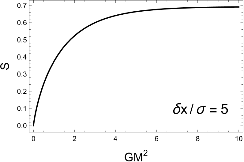
A similar analysis can be performed in a time-dependent case, where, for illustration, we considered a quantum harmonic oscillator in a Gaussian state that emits gravitational waves, see [33, 55]. We can ask a similar question about the overlap of the coherent state of the gravitons emitted during the oscillations. We have shown this computation in Appendix. B.

In this paper, we have shown that when we treat matter and the graviton on an equal footing, the graviton vacuum evolves to a coherent state. The displaced vacuum yields a classical geometry, where the individual, left, and right half of the matter superposition yields a geometry equivalent to a superposition of a Schwarzschild geometry, as shown in Eq. (30) in a perturbative treatment of gravity.

Furthermore, we have shown the quantum overlap, which we may call a quantum bridge, between the two coherent states of the graviton changes with mass, superposition size, and the width of the individual mass density profile. In this analysis, we ignored the time-dependent aspects; however, these can be added in the future, and there will also be a dependence on the momentum of the individual wave packets that create the matter-wave superposition.

In Appendix. B, we present a similar computation in a time-dependent setting for a quantum harmonic oscillator. Such a system emits gravitational waves, and we computed the overlap of the displaced vacuum of the gravitons in the transverse-traceless gauge.

The results of the paper shed light on how matter-graviton coupling provides the quantum overlap between quantum geometries lead by the displaced vacuum of the gravitons at a perturbative level in a spatial superposition of matter. The results corroborate the results of the papers that show how to witness this quantum superposition of geometry via entanglement witness [16]. Note that we cannot conjecture beyond the tree level, as higher order terms, such as post-Newtonian contributions and higher order vertex corrections will need to be taken into account to go beyond the computations we have performed in this paper. At a perturbative level our computations of the overlap/contrast between the geometries during quantum spatial superposition provide a hint how quantum gravity may pave out in reality when the non-perturbative effects are taken into account, which are indeed hard questions and demand a non-perturbative treatment of gravity.

Acknowledgements: A.M.’s research is funded by the Gordon and Betty Moore Foundation through Grant GBMF12328, DOI 10.37807/GBMF12328. This material is based on work supported by the Alfred P. Sloan Foundation under Grant No. G-2023-21130. T.Z. is supported by the China Scholarship Council (CSC).

References

- [1] (2016) . Note: https://www.youtube.com/watch?v=0Fv-0k13s_kAccessed 1/11/22 Cited by: §I.
- [2] (2019-08) Stern-gerlach matter-wave interferometer. Phys. Rev. Lett. 123, pp. 083601. External Links: Document, Link Cited by: Appendix B.
- [3] (2013) A Master Equation for Gravitational Decoherence: Probing the Textures of Spacetime. Class. Quant. Grav. 30, pp. 165007. External Links: 1305.5231, Document Cited by: §I.
- [4] (1996) Quantum theory of nonrelativistic particles interacting with gravity. Phys. Rev. D 54, pp. 1600–1605. External Links: gr-qc/9511004, Document Cited by: §I.
- [5] (2014) Testing the limits of quantum mechanical superpositions. Nature Physics 10 (4), pp. 271–277. External Links: Document Cited by: §I.
- [6] (1999) Wave–particle duality of c60 molecules. Nature 401 (6754), pp. 680–682. External Links: Document Cited by: §I.
- [7] (2017) Phase shift in an atom interferometer due to spacetime curvature across its wave function. Physical review letters 118 (18), pp. 183602. External Links: Document Cited by: §I.
- [8] (2017) Phase Shift in an Atom Interferometer due to Spacetime Curvature across its Wave Function. Phys. Rev. Lett. 118 (18), pp. 183602. External Links: 1610.03832, Document Cited by: §I.
- [9] (2023) Quantum entanglement of masses with nonlocal gravitational interaction. Physical Review D 107 (12), pp. 124036. External Links: Document Cited by: §I, footnote 2.
- [10] (2018) Quantum Superposition of Massive Objects and the Quantization of Gravity. Phys. Rev. D 98, pp. 126009. External Links: Document Cited by: §I.
- [11] (2024-05) Comparing the decoherence effects due to black holes versus ordinary matter. External Links: 2405.02227 Cited by: §I.
- [12] (2023) Gravitational optomechanics: Photon-matter entanglement via graviton exchange. Phys. Rev. D 108 (6), pp. 064023. External Links: 2209.09273, Document Cited by: §I.
- [13] (2012) Towards singularity and ghost free theories of gravity. Phys. Rev. Lett. 108, pp. 031101. External Links: 1110.5249, Document Cited by: §II.
- [14] (2013) Nonlocal theories of gravity: the flat space propagator. In Barcelona Postgrad Encounters on Fundamental Physics, pp. 13–24. External Links: 1302.0532 Cited by: §II.
- [15] (2013-07) Effective field theory approach to gravitationally induced decoherence. Phys. Rev. Lett. 111, pp. 021302. External Links: Document, Link Cited by: §I.
- [16] (2017) Spin Entanglement Witness for Quantum Gravity. Phys. Rev. Lett. 119 (24), pp. 240401. External Links: 1707.06050, Document Cited by: §I, §III, §V.
- [17] (2022) Mechanism for the quantum natured gravitons to entangle masses. Phys. Rev. D 105 (10), pp. 106028. External Links: 2201.03583, Document Cited by: §I, §II, §II, footnote 2.
- [18] (2023) Entanglement Witness for the Weak Equivalence Principle. Entropy 25 (3), pp. 448. External Links: 2203.11628, Document Cited by: §I.
- [19] (2021) Gravitons in a box. Physical Review D 104 (6), pp. 066019. External Links: Document Cited by: Appendix B.
- [20] (2022) Infrared scaling for a graviton condensate. Nuclear Physics B 977, pp. 115730. External Links: Document Cited by: Appendix B, Appendix B.
- [21] (2025-09) A Spin-Based Pathway to Testing the Quantum Nature of Gravity. External Links: 2509.01586 Cited by: §I.
- [22] (1994-06) Noise and fluctuations in semiclassical gravity. Physical Review D 49 (12), pp. 6636–6655. External Links: ISSN 0556-2821, Link, Document Cited by: §I.
- [23] (2019) Tabletop experiments for quantum gravity: a user’s manual. Class. Quant. Grav. 36, pp. 034001. External Links: Document, Link Cited by: §I.
- [24] (2022) Newton, entanglement, and the graviton. Phys. Rev. D 105 (2), pp. 024029. External Links: 2108.06320, Document Cited by: §I.
- [25] (2023) Distinguishing jordan and einstein frames in gravity through entanglement. Physical Review D 108 (12), pp. L121505. External Links: Document Cited by: §I.
- [26] (2023) Locally mediated entanglement in linearized quantum gravity. Physical Review Letters 130 (10), pp. 100202. External Links: Document Cited by: §I.
- [27] (2019) On the possibility of laboratory evidence for quantum superposition of geometries. Physics Letters B 792, pp. 64–68. External Links: Document Cited by: §I.
- [28] (1975-06) Observation of gravitationally induced quantum interference. Phys. Rev. Lett. 34, pp. 1472–1474. External Links: Document, Link Cited by: §I.
- [29] (2022) Black holes decohere quantum superpositions. Int. J. Mod. Phys. D 31 (14), pp. 2241003. External Links: 2205.06279, Document Cited by: §I.
- [30] (2022) Gravitationally mediated entanglement: Newtonian field versus gravitons. Phys. Rev. D 105, pp. 086001. External Links: Document Cited by: §I.
- [31] (2023) Killing horizons decohere quantum superpositions. Phys. Rev. D 108 (2), pp. 025007. External Links: 2301.00026, Document Cited by: §I.
- [32] (2015-02) Decoherence induced by long wavelength gravitons. Phys. Rev. D 91, pp. 044038. External Links: Document, Link Cited by: §I.
- [33] (1986) Introduction to gravitation. World Scientific Publishing Company. Cited by: §I, §IV.
- [34] (1994) General relativity as an effective field theory: The leading quantum corrections. Phys. Rev. D 50, pp. 3874–3888. External Links: gr-qc/9405057, Document Cited by: §I.
- [35] (2013) Matter-wave interference with particles selected from a molecular library with masses exceeding 10000 amu. Phys. Chem. Chem. Phys. 15, pp. 14696–14700. External Links: 1310.8343, Document Cited by: §I.
- [36] (1988) Is spin coherence like humpty-dumpty? i. simplified treatment. Foundations of Physics 18 (10), pp. 1045–1056. External Links: Document Cited by: §I.
- [37] (2019) Quantum superposition of molecules beyond 25 kDa. Nature Phys. 15 (12), pp. 1242–1245. External Links: Document Cited by: §I.
- [38] (2007) Atom interferometer measurement of the Newtonian constant of gravity. Science 315, pp. 74–77. External Links: Document Cited by: §I.
- [39] (1952-08) Quantization of einstein’s gravitational field: general treatment. Proceedings of the Physical Society. Section A 65 (8), pp. 608. External Links: Document, Link Cited by: §I, §II, §II, §II, §II.
- [40] (2014-02) A universal matter-wave interferometer with optical ionization gratings in the time domain. Nature Phys. 9, pp. 144. External Links: 1402.1364, Document Cited by: §I.
- [41] (2015) Quantum superposition at the half-metre scale. et.al, Nature 528, pp. 530–533. External Links: Link Cited by: §I.
- [42] (2013/09/09/online) Coherent stern–gerlach momentum splitting on an atom chip. Nature Communications 4, pp. 2424. External Links: Link Cited by: Appendix B.
- [43] (2021) Realization of a complete stern-gerlach interferometer: toward a test of quantum gravity. Science advances 7 (22), pp. eabg2879. External Links: Document Cited by: Appendix B, §I.
- [44] (2017) Gravitationally induced entanglement between two massive particles is sufficient evidence of quantum effects in gravity. Phys. Rev. Lett. 119, pp. 240402. External Links: Document Cited by: §I.
- [45] (2020) Locality and entanglement in table-top testing of the quantum nature of linearized gravity. Physical Review A 101 (5), pp. 052110. External Links: Document Cited by: §I.
- [46] (2022) Constructing nano-object quantum superpositions with a Stern-Gerlach interferometer. Phys. Rev. Res. 4 (2), pp. 023087. External Links: 2105.01094, Document Cited by: Appendix B.
- [47] (2017-10) Quantum coherence, radiance, and resistance of gravitational systems. Phys. Rev. D 96, pp. 084014. External Links: Document, Link Cited by: §I.
- [48] (2020-07) The noise of gravitons. International Journal of Modern Physics D 29 (14), pp. 2042001. External Links: ISSN 1793-6594, Link, Document Cited by: §I.
- [49] (2026) Probing quantum mechanics with nanoparticle matter-wave interferometry. Nature 649 (8098), pp. 866–870. External Links: Document Cited by: §I.
- [50] (2020) Motional dynamical decoupling for interferometry with macroscopic particles. Phys. Rev. Lett. 125, pp. 023602. External Links: Document, Link Cited by: Appendix B.
- [51] (2025) Genuine tripartite entanglement in graviton-matter interactions. Phys. Rev. A 111 (2), pp. 022444. External Links: 2411.03293, Document Cited by: §I.
- [52] (2014) Interferometry with atoms. La Rivista del Nuovo Cimento 37 (10), pp. 509–589. External Links: Document Cited by: §I.
- [53] (1988-06) Is spin coherence like Humpty-Dumpty?. Zeitschrift fur Physik D Atoms Molecules Clusters 10 (2-3), pp. 135–144. External Links: Document Cited by: §I.
- [54] (1989-08) Spin coherence and humpty-dumpty. iii. the effects of observation. Phys. Rev. A 40, pp. 1775–1784. External Links: Document, Link Cited by: §I.
- [55] (2024) Loss of coherence and coherence protection from a graviton bath. Physical Review D 109 (8), pp. 084050. External Links: Document Cited by: Appendix B, §I, §I, §IV.
- [56] (2021) Relative acceleration noise mitigation for nanocrystal matter-wave interferometry: Applications to entangling masses via quantum gravity. Phys. Rev. Res. 3 (2), pp. 023178. External Links: 2007.15029, Document Cited by: §I.
- [57] (2016) Tolerance in the Ramsey interference of a trapped nanodiamond. Phys. Rev. A 93, pp. 043852. External Links: Link Cited by: Appendix B.
- [58] (2016) Free nano-object Ramsey interferometry for large quantum superpositions. Phys. Rev. Lett. 117, pp. 143003. External Links: Link Cited by: Appendix B.
- [59] (1979) EFFECT OF EARTH’S ROTATION ON THE QUANTUM MECHANICAL PHASE OF THE NEUTRON. Phys. Rev. Lett. 42, pp. 1103–1106. External Links: Document Cited by: §I.