Branching Brownian motion with rank-based selection and reaction-diffusion equations
Abstract
We consider a family of branching-selection particle systems in which particles branch at time dependent rate and are killed with a probability which is dependent on their rank via some function . We show that, under fairly minimal conditions, the hydrodynamic limit of such a system is given by the reaction-diffusion equation with nonlinearity which is a function of . This is a significant generalisation of the well-studied -BBM process, and is similar to the family of ‘-BBM’ processes described by Groisman & Soprano-Loto in [rankDependentBBM]. On the one hand, this allows us to understand common reaction-diffusion equations as limits of interacting particle systems with simple description. On the other hand, the asymptotic behaviour of solutions of the reaction-diffusion the PDEs can help us predict the asymptotic properties of the associated particle systems. We give general conditions under which the branching-selection particle system has an asymptotic velocity, and describe the velocity up to order ; furthermore, we describe the connection between this velocity and the spreading speeds and travelling waves of the corresponding reaction-diffusion equation. This provides a partial weak selection principle.
1 Introduction
Reaction diffusion equations are a broad class of partial differential equations, which find applications in a number of areas of physical sciences, including ecology, cell biology, and flame propagation. We consider reaction-diffusion equations of the general form:
where . A well-known example is the F-KPP equation, which was first studied in the 1930s independently by Fisher [11] and Kolmogorov, Petrovskii, and Piscunov [16] in the context of population genetics. The F-KPP equation is an equation of the form with , for , and for ; a typical example being the Fisher equation . An important property of the F-KPP equation is the existence of travelling wave solutions and travelling fronts; it is well known that the F-KPP equation has a travelling wave solution for every speed . Thus the Fisher equation has travelling wave solution for all speeds . The situation is more complex in the general case, when is not positive everywhere on .
The PDE can also be understood as the hydrodynamic limit of an interacting particle system [13] which can be described as follows: consider particles moving on as independent Brownian motions. At rate , draw uniformly at random two particles from the population and move the leftmost of the two particles to the location of the rightmost particle.
Groisman and Soprano-Loto later generalised this when they describe their so-called ‘-BBM’ process. In the -BBM, particles behave as independent Brownian motions on , with branching described by the function and deletion by the increasing function . More precisely, the th leftmost particle branches at rate , where is the number of particles in the system at time . Simultaneously to the th particle branching, the th leftmost particle, where , is killed with probability and this includes the possibility that no particle is deleted. The family of processes they describe is relatively general, and in particular includes branching Brownian motion (BBM), and the fixed population size -BBM process (see [3],[6],[17]), among many others. In their work, they conjecture that the particle system has the hydrodynamic limit:
where is the limiting empirical density and the corresponding cumulative distribution.
Another generalisation of the -BBM is studied by Atar [1], who considers an injection-branching-selection system, in which the branching and selection steps are decoupled. The system proposed in [1] starts with Brownian motions on , each branching at rate , and subsequently particles are added to the system (injected) according to a random point process and leftmost particles are deleted according to a random process . As with the -BBM, this setup allows for a variable number of particles. Subsequently Atar describes a weak formulation of the corresponding hydrodynamic limit.
In this paper we study a branching-selection particle system with rank-dependent selection which can be described as follows. particles move as independent Brownian motions on , and each particle branches into two particles independently at time dependent rate . Simultaneously with each branching event, we kill a particle, killing the th leftmost particle with probability , where is a positive, bounded, and continuous function with . We will call this process the -BBM. Note that unlike the -BBM, this allows for the rank of the deleted particle to be greater than the rank of the branching particle. Then we will show that the empirical cumulative distribution function of the -BBM process converges to the unique solution to the following reaction-diffusion PDE:
| (1) |
The consequences of this result are two-fold. Firstly, any PDE , where and for can be understood as the hydrodynamic limit of a -BBM with branching rate and selection function . Secondly, we may consider functions for which the asymptotic behaviour of the equation is known, and discover what this implies about the asymptotic behaviour of the corresponding interacting particle system. Examples are given in Section 6.
Another question about the -BBM which naturally arises is that of its asymptotic velocity. By coupling the process to versions of the -BBM process, we prove that, when and under certain conditions on , its asymptotic velocity, , matches that of the -BBM up to order . That is,
We may notice that when , , and and for all , then is the minimal travelling wave speed for the PDE (1). This is an example of a weak selection principle; the particle system has an asymptotic velocity which ‘selects’ the minimal travelling wave speed of the limiting PDE as . See for example [3], [6], [14]. Thus we aim to the answer the question of when the following diagram holds:
A discussion of this appears in Section 6.
2 Construction of the process
Before stating the main results of this paper, we will formally construct the -BBM process as a measure-valued random process constructed from i.i.d Brownian motions, a Poisson process, and discrete random variables. We will write where is the vector of locations of the particles at time . Define the function to be the function which sorts an dimensional vector into increasing order. Furthermore, let denote the th element of the vector , which is the th smallest element of the vector .
Let the initial condition where is an atomic measure, the sum of atoms of weight , and suppose that converges weakly to the probability measure which is absolutely continuous with respect to the Lebesgue measure.
Now let be a Poisson process with time-dependent intensity , where is continuous and bounded. Let be the discontinuities of the process, with . At each time we will order the elements of so that , but we may have for and . Let be a sequence of i.i.d. uniform random variables on , and let be a sequence of i.i.d. random variables with for , where is assumed to be positive and continuous with .
Let be a family of i.i.d Brownian motions. On each interval for , the particle at location is driven by the Brownian motion ; so when , the particles of the system are at locations for . Then at each time , we move the particle at location to the location of . Note that this does not exclude the possibility that . Repeating this inductively, we can describe the process as a function for all times . Thus we have constructed the measure-valued process .
2.1 Notation
-
•
denotes the Heaviside function and its reflection.
-
•
is the set of functions such that , , and exist, and , , , and are continuous and bounded, and is the subset of vanishing as the first variable goes to . will denote the set of continuous and bounded functions on of which the functions that are constant in the second variable form a dense subset. denotes the set of continuous functions with continuous derivatives , , and and compact support.
-
•
For function and measure , and for functions , .
-
•
For martingale , denotes the quadratic variation process of .
-
•
For set , will denote the set of probability measures on .
-
•
will denote the space of finite measures on under the weak topology. Moreover, we write for the extended real line which is the two-point compactification of , and for the corresponding space of measures.
-
•
We will write to denote that the measure is absolutely continuous with respect to the Lebesgue measure .
3 Main results
The first result we prove here is the hydrodynamic limit for the -BBM process under the conditions that is continuous and bounded and is positive, and continuous on , with . We will show, in a sense which we will make clear, that the hydrodynamic limit of the process -BBM is the unique classical solution of the PDE:
| (2) |
It is a classical result due to Kolmogorov, Petrovskii, and Piscunov (§3, Theorem 1, [16]) that if is continuous, bounded, and Lipschitz continuous in the first and third variable, and is bounded and continuous, then has a unique classical solution. Note that if is continuous and bounded on and is positive and continuous on , then
immediately satisfies these conditions.
Let us now define the assumption (A1) on and under which our first main result holds.
(A1): , and satisfy assumption (A1) if is continuous with and is continuous and bounded.
Theorem 1.
Let be the empirical measure-valued process corresponding to the -BBM process with . Let denote the distribution of . Then under assumption (A1), for any fixed , converges weakly to , where is a Dirac mass on , and is the unique classical solution to (2) with initial condition .
Next we define assumption (A2), which is a sufficient condition on and for the -BBM process to have an asymptotic velocity .
(A2): and satisfy assumption (A2) if for for some and for for some , and .
By coupling our system to the -BBM process, we can show that agrees with the speed of the -BBM up to order .
Theorem 2.
Let be a -BBM with any initial configuration. Then under the assumption (A2), the -BBM has asymptotic velocity:
We may reasonably ask what happens if assumption (A2) fails. If the assumption that for is broken, then we never kill the leftmost particles of the -BBM, and accordingly, we would expect as so that no positive asymptotic speed exists. One the other hand, if for , then the rightmost particles are killed at strictly positive rate, and we would expect this to slow down the rightmost particle so that . We do in fact expect that if as sufficiently quickly, then there is still an asymptotic velocity close to (see Conjecture 12), however the specific method of our proof does not apply in this setup.
In order to form a weak selection principle, we also wish to relate to the travelling wave speed or spreading speed of the PDE (2). This is made precise in Section 6, and summarised in the following Theorem.
Theorem 3.
4 Hydrodynamic limit
In this section, we will prove the hydrodynamic limit result of Theorem 1. The following gives an outline of the proof strategy, which was inspired by Demircigil and Tomasevic [7].
First we will give a probabilistic representation of tested against a test functions in . We allow the test functions to depend on time as this will allow us to easily prove uniqueness of weak solutions in step 3 (Proposition 11).
Proposition 4.
Let be the measure-valued Markov process corresponding to the -BBM process. Let . Then , and satisfy the following equation:
| (3) | ||||
where is a continuous local martingale with for fixed , and is a local martingale with for fixed .
Proof.
Note that for an atomic measure such as we have . Then by Ito’s formula, for :
so for
Then at the time , the discontinuity in induces a change in (unless ). Specifically, jumps by . Thus
and therefore, for general , integrating with respect to , we can write
| (4) | ||||
where is the continuous local martingale . Now note the process is a compensated Poisson process and thus a martingale Then we wish to show that the process
is a local martingale with respect to the filtration . This follows from that fact that the random variables and are independent of , so that:
where the final equality follows from the fact that is a martingale and hence is a martingale. From this it follows that , thus confirming that is a local martingale. So equation (4) can be written as
We will now deal with the final term of the above equation - the sum over - in two parts. Using the observation that for all , and summing first over , we can calculate that
Then observing that , and summing first over , we have
Putting this together yields equation (3), as required. Note that by Ito’s isometry and the independence of the ’s, has expected quadratic variation
| (5) |
Since is bounded, thus as for any fixed . Furthermore, by Ito’s isometry, the expected quadratic variation of can be calculated:
| (6) |
Since and is bounded, thus for fixed . This concludes the proof. ∎
Next, we prove tightness of the sequence of laws of . Specifically, we will prove that the sequence of laws is tight in the space , where is the extended real line . The benefit of this method is that is compact, and as a consequence is a compact subset of . This will help us to prove a compactification condition required to show tightness.
Proposition 5.
Fix , and let denote the law of . Then the sequence of is tight in with respect to the Skorokhod metric.
Proof.
In order to show that the sequence is tight in with respect to the Skorokhod topology, it is sufficient (Theorem 1.18, [9]) to show the following conditions:
-
(i)
Compact containment: For all there exists a compact subset such that inf_N∈N P(μ_t^N ∈K_ϵ ∀ t∈[0,T])¿1-ϵ
-
(ii)
Tightness of real-valued processes: The sequence of laws of is tight in for every function in a dense subset of
Observe that the subset , the subset consisting of probability measures, is a compact subset since is itself compact. This is easily seen by observing that any subset of is tight, since is a compact subset of such that for all . Then since for all and , the compact containment condition (i) holds immediately.
We now prove condition (ii). Since each has support on , thus it is sufficient to show that is tight for all functions in a dense subset of . We choose to be our dense subset of . By Aldous’ tightness criterion (see, for example, Theorem 16.10, [4]), is tight if the following conditions hold:
-
A
For every , .
-
B
For each , there exists such that if , , and is a stopping time such that , then .
Condition A follows immediately by observing that , therefore since is bounded, then for , this probability is . Now let us prove condition B. Since , thus , and , , and are all bounded for , say by a constant . So (3) gives that
Therefore by Markov’s inequality and the Burkholder-Davis-Gundy inequality, there exists a constant such that:
Therefore condition B follows, hence the sequence is tight, thus proving condition (ii), and completing the proof. ∎
A very similar method to the above is employed by Etheridge (Section 1.4, [9]). To prove the compact containment condition, they instead uses the one-point compactification of , , instead of (the two-point compactification of ). However, since and are not distinguished in , continuous bounded functions must have . However we wish to have convergence of for functions with , which is why we use instead.
This generalisation from to will not cause any additional difficulties for us. Since is tight, therefore by Prokhorov’s theorem (Theorem 5.1, [4]), there is a weakly convergent subsequence . By appealing to a comparison with branching Brownian motion, we can show that any subsequential limit is absolutely continuous with respect to the Lebesgue measure and has for all times almost surely.
Lemma 6.
Let be a subsequential limit of and let . Then and for all -a.s.
This proof essentially follows from the fact that the -BBM can be bounded above by a branching Brownian motion started from particles, which has a well known hydrodynamic limit which is absolutely continuous with respect to the Lebesgue measure for all .
Proof.
We construct the -BBM from a branching Brownian motion as follows. Consider a branching Brownian motion starting from particles according to the initial configuration which branches at time-inhomogeneous rate . Let denote the set of particles at time , and be the subset of consisting of the descendants of the particle which starts at location . Now we will colour the particles of the BBM blue and red. Initially, all particles are blue. Then at each branching time of a blue particle, we colour exactly one blue particle red; the th leftmost blue particle being coloured red with probability . Subsequently, blue particles always branch into blue particles and red into red. Clearly there are always exactly blue particles, and the subset of blue particles describes a -BBM.
Now let be the rescaled empirical measure of this coloured BBM process at time . It is well-known (and proven in the Appendix, Theorem 16, for completeness) that if is the law of , then converges weakly to , and if , then has density -a.s., and is the unique classical solution to the PDE . Therefore since and for all -a.s., and is dominated by for all , thus and for all -a.s.. ∎
Since we know that has no mass at , convergence in the space implies convergence in the space , which is what we use from here onwards. Next we show, by Kolmogorov’s continuity criterion, that the map is continuous on -a.s.. In particular:
Lemma 7.
Let be a subsequential limit of and let . Then the map is continuous on with respect to the weak topology -a.s..
Proof.
Since is cadlag, we will show using the Kolmogorov continuity theorem to show that there exists a continuous modification of , and therefore as a result is almost surely continuous (see Theorem 1, [20]). So fix and . By the definition of convergence in the Skorokhod topology on , there exists a sequence of functions such that and converge to as . Therefore by Fatou’s lemma:
As in the proof of Proposition 5, using the representation (3), we can bound
for some constant . Then by (5) and (4) and the Burkholder-Davis-Gundy inequality, and converge to as , therefore:
since . Therefore satisfies the conditions of the Kolmogorov continuity theorem, therefore has a continuous modification, and thus is almost surely continuous (Theorem 1, [20]). Therefore is continuous for all in a countable dense subset of almost surely, and hence is continuous with respect to the weak topology almost surely. ∎
Next we prove that each subsequential limiting distribution is concentrated on the weak solutions of a deterministic PDE.
Proposition 8.
Let be a sub-sequential limit of , and let . Then for any , satisfies -a.s. the equation
| (7) |
In particular, (7) is the weak formulation of the non-linear equation:
which describes the limiting density of the process. We will subsequently transform this into its integrated version, the PDE (2) which describes the limiting cumulative distribution function.
Proof.
Without loss of generality, throughout this proof, we will consider the sub-sequential limit to be labelled . For measure-valued process , function , integer , and time , define:
Therefore by Proposition 4, . Now . Therefore by (5), (4), and the Burkholder-Davis-Gundy inequality, for every fixed :
| (8) |
Now by the Skorokhod representation theorem, there exists a sequence of random variables and defined on the same probability space , such that converges -a.s. to in the Skorokhod topology, with and . By Lemma 7, the map is continuous on -a.s. Next we will prove that as -a.s., which is a simple consequence of continuity and convergence in the Skorokhod topology. By the triangle inequality, for
The first term converges to almost surely by the Skorokhod convergence of , and the second term converges to almost surely by the almost sure continuity of at . Since , it immediately follows that for we have and .
Note that for , since is bounded and continuous, thus is bounded and continuous. Thus converges to for all -almost surely. Therefore by the dominated convergence theorem
Extending the idea of the previous argument, since and are true for all -a.s., define the measure set
We will show that for , the convergence
| (9) |
holds. Fix . We will also fix , however we omit to explicitly show dependence of for readability. Since the integrand of the left-hand side of (9) is bounded by , therefore by the dominated convergence theorem:
By the triangle inequality
| (10) | ||||
| (11) | ||||
| (12) |
Since is continuous and is compact, there exists such that implies that for all , we have for all . Therefore for :
This proves that (10) converges to as . Next we tackle (11). Since converges weakly to and , thus for all as . By continuity of , converges to for all . Moreover, since , therefore by Prokhorov’s theorem (Theorem 5.1, [4]), , is tight, therefore we can choose a compact set such that for all . So
Then since is compact, converges to uniformly on as . Then since and are bounded, there exists such that implies
for all , and therefore for any probability measure , we have that implies
Therefore, by the triangle inequality, for , we have that
This proves convergence of (11). Finally we tackle (12). Observe that is continuous and bounded in , therefore by the Portmanteau theorem, since , we have
So let be such that implies that
thus for , we have that:
Therefore (9) holds for all , hence -almost surely. Therefore for any suitable test function , we have
| (13) | ||||
Fixing and , and recalling the boundedness of each term of , we can observe that the sequence is bounded uniformly in . Hence is uniformly integrable. Then since convergence in expectation and uniform integrability imply almost sure convergence (see for example Appendixes, Proposition 2.3 in [10]).Therefore (8) yields that -a.s., completing the proof. ∎
Next, we show the deterministic result that any solution of (7) with has for all .
Proposition 9.
Let satisfy equation (7) with . Then for any .
Proof.
We will prove that by showing that such that for any interval , we have , since this shows that is Lipschitz continuous, a strictly stronger condition than absolute continuity. So fix and . Let and be the heat kernel. Since , say has density (i.e. ), and let be a sequence of mollifiers such that is a monotonic increasing sequence converging pointwise to as .
We define as a sequence of test functions . This is the solution of the backward heat equation on with terminal condition ; that is and . Plugging this into (7), we yield:
| (14) |
Now since is a monotonically increasing sequence converging to thus using the monotone convergence theorem and Fubini’s theorem
As is positive and bounded, we can bound , and hence taking limits in equation (14) and applying the monotone convergence theorem again to the integral term, we yield
so that Grönwall’s inequality gives . This holds for any interval , hence . ∎
Next we show that if satisfies (7), then is the weak solution of the PDE (2). As we do not yet know that the function is differentiable either in or we cannot yet say that it is a classical solution. Consider taking a classical solution of (2), then multiplying by a test function and integrating over yields:
| (15) |
and then switching the derivatives from to gives
and
therefore equation (15) could be written:
| (16) | ||||
Notice that no assumptions on the differentiability of are required in equation (16). This is the natural definition for a weak solution of equation (2).
Definition 1.
Proposition 10.
Suppose that satisfies (7); that is
for every . Define . Then for all and satisfies
| (17) | ||||
for all test functions such that .
Proof.
Firstly we show that any solution of (7) such that and has for all . Substituting into (7) and differentiating, we get that
Since is absolutely continuous with respect to the Lebesgue measure, therefore its cumulative distribution function is continuous in , and is a measurable function and has a well-defined inverse with respect to . Define by the pushforward measure of by , which is the Lebesgue measure on (see Example 3.6.2 of [5], for example). So by Theorem 3.6.1 of [5], we have that:
Therefore solves the ordinary differential equation with , and therefore , as desired. Now recall that we have the relations , , and . So by Fubini’s theorem, we have
Again, using Theorem 3.6.1 of [5], we have that:
Therefore
and hence for such that :
∎
Note that the functions with compact support such that form a dense subset of , so the above proposition shows that is in fact a weak solution of the PDE (2). Next we show that the weak formulation (17) has a unique solution.
Proposition 11.
Fix and . Then there is at most one function solving (17) for all such that , with , and such that is continuous in for all
Proof.
Suppose that both solve (17) and are both continuous in for all . Define their difference which is also continuous in . Now fix and let be a test function which is positive and smooth with compact support and total mass . Then let be the solution of the backward heat equation with terminal condition . Therefore (17) yields
| (18) |
Then as is bounded,
Therefore as is bounded and for all , therefore (18) gives that
Now let us consider the supremum of over all smooth positive functions with total mass . Clearly , so the supremum is clearly bounded by . On the other hand, since is continuous, choosing as a smooth approximation to , where is the point at which ’s supremum is achieved, we can clearly choose such that is arbitrarily close to . Thus . Therefore we have:
and so by Grönwall’s inequality, it follows that for , and so . Thus (17) has a unique solution which is continuous in . ∎
Proof.
(Of Theorem 1) By tightness (Proposition 5) the sequence of laws has subsequential limits. By Proposition 8, if is a subsequential limit and , then is a weak solution to the PDE (7). Moreover, since , Proposition 9 tells us that for all . Therefore by Propositions 10 and 11, is the unique solution to (17); that is, the unique weak solution to (2). Then as (2) has a unique classical solution (§3, Theorem 1, [16]) this coincides with the unique weak solution. Since, therefore, all subsequential limits of are the same (i.e. a Dirac mass at , where is the unique classical solution to (2)), thus the sequence converges weakly to this limit. ∎
Let us conclude this section with a remark about the necessity of the assumption (A1). Note that he -BBM can be described as -BBM process where and , since at each branching time, we select the leftmost particle to be deleted with probability . Such a certainly fails the assumption, since is not even a function. And indeed, the boundedness of is crucially utilised in the proofs of Propositions 4, 5, and Lemmas 6, 7, and continuity is needed in the proof of Prposition 8. Unfortunately, therefore, it is non-trivial to see how the methods here would, without non-trivial extension, reproduce the hydrodynamic limit result of [6].
5 General reaction-diffusion equations
So far we have shown that the -BBM process has a hydrodynamic limit described by the unique solution to the reaction-diffusion equation
In particular, this means that given any function with and , we can describe the solution of the PDE as the hydrodynamic limit of a branching-selection particle system with selection function defined by . The author hopes that this introduces an intuitive way in which to understand a number of general reaction-diffusion equations, since can be thought of as describing the relative probability of an individual in the population being out-competed as a function of ranked fitness.
Example 1:
A ubiquitous choice of is the Fisher equation, when , which has been studied since it was introduced by Fisher [11]. Choosing gives us a particle system who’s hydrodynamic limit is the equation . Simply, this particle system is the system of particles, moving as Brownian motions, in which each particle branches at unit rate and simultaneously a particle is deleted with a probability which is directly proportional to its rank.
Example 2:
The Allen-Cahn equation , for , models the strong Allee effect. In this case, to realise the PDE as the hydrodynamic limit of a rank-dependent branching selection system, we choose
Example 3:
Another common example we give is , with . In this case, we can realise as the hydrodynamic limit of the rank-dependent branching selection system with selection function .
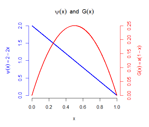
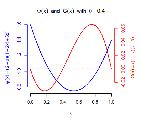
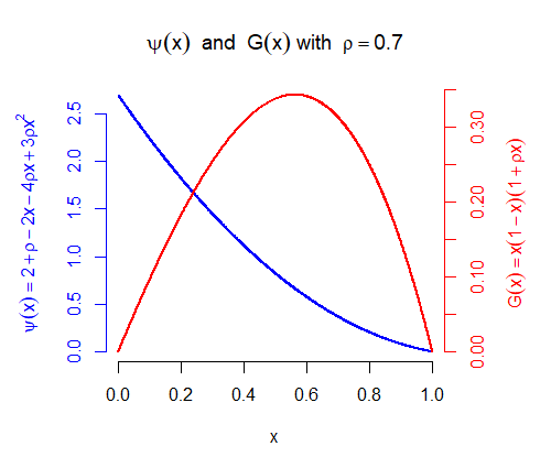
Example 4:
Let us consider another way in which the PDE connection may be insightful. Consider a branching-selection particle system with rank-dependent selection such that particles of intermediate rank are deleted, whereas particles of extreme ranks (ie. close to or ) are never deleted. What should we expect the behaviour of such a particle system to be?
Since the ‘middle’ particles are deleted but both extremes do not get deleted, we expect that the system will split into two clouds of particles, one travelling to and one to . But what proportion of particles is in each cloud? For a concrete example, consider , where is a scaling constant so that . So the leftmost and rightmost of particles are never killed. We should expect there to be more particles in the left-moving cloud than in the right-moving cloud, but by how many?
Consider the corresponding reaction-diffusion equation with . This is a monostable source term, with a single stable zero at the value such that . For this example, . Therefore for any initial condition such that and , the solution to the PDE (2) tends everywhere to as , leaving us with mass at and mass at .
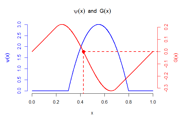
Thus we expect roughly of the particles to converge to and of the particles to converge to .
6 Weak selection principle
In this section we prove Theorems 2 and 3. First we prove Theorem 2 by constructing couplings between the -BBM and the -BBM process, whose asymptotic velocity is known (see Appendix of [18]). The idea for this proof is due to Paul de Lambert des Granges and produced here with his permission. Recall that we are trying to prove the following:
Theorem.
Let be a -BBM with any initial condition. Then under assumption (A2), the -BBM has asymptotic velocity:
Proof.
We will prove the above proposition by coupling the -BBM above and below to an -BBM process. It is known (Theorem 21, [18]) that the -BBM has asymptotic velocity .
Now let be a -BBM process constructed as in Section 2. We will couple an upper-bounding -BBM process to as follows. Initially, . As in the construction of the -BBM, let , and let be the times of discontinuity of the Poisson process so that at time , the th leftmost particle of moves to the location of the th leftmost. Suppose for induction that is constructed up to time and that for . Then on , drive the particle of which is at location by the Brownian motion . Since is also the Brownian motion which drives the particle of at location , clearly implies that for . Now at the stopping time , we branch the th leftmost particle of and simultaneously delete the leftmost particle of .
For a vector and , define the function to be the function which deletes the th element and duplicates the th element of the vector . That is,
where is not necessarily smaller than . With this definition, we have that and we define . Then observe that and implies that . In layman’s terms, deleting a particle which sits more to the left succeeds in making the whole system sit more to the right. Therefore , and hence by induction for all . Thus:
Next we construct a lower bound. Consider constructing a -BBM with particles, , as follows. Let denote the location of the th leftmost particle of , and initially define for . So the particles of have the same locations as the rightmost particles of . Let denote be the vector of positions of the rightmost particles of . Similarly to before, assume for induction that is constructed up to time and that for . Then construct for as follows. On the interval , drive the particle of which is at location at time by the Brownian motion ; that is, we couple the particles of to the rightmost particles of . Thus implies that for . Then at the time , the th leftmost particle of moves to the location of the th leftmost particle. If , then we branch the th leftmost particle of and simultaneously delete the leftmost particle in the system; otherwise, we do nothing. By assumption (A2), on , so , which is to say that we never delete one of the rightmost particles of at a branching/deletion time.
Clearly if we do nothing, then . Consider on the other hand the case that a particle of branches at time . Again, by assumption (A2), on , thus the particle of which is deleted is not among the rightmost. Therefore consists of the rightmost particles of , with the th of those duplicated. Since similarly consists of the rightmost particles of , with the th duplicated, we can conclude that implies . Therefore by induction it holds that for all .
Now observe that, by our construction, the process is simply an -BBM process with particles, therefore
It remains to show that the limits and are equal. To do this, we consider the following events which we can think of as ‘regeneration events’. For , define
This is the event that in the time interval , there are exactly branching times, , at all of which the rightmost particle branches. We can explicitly calculate . Define and , so that . Recall from our construction of the -BBM that, in between branching events, the particle which was the th leftmost at the most recent branching event is driven by the Brownian motion . Then define
Note this event is defined so that for some independently of and the configuration of . Finally, let
be the event that all branching events in , the leftmost particle is deleted. Since for all , this happens with positive probability; we can explicitly calculate .
Now define . Therefore for some independently of and the configuration of . Now let us consider the configuration of particles of at time on the event . Since for all , this means that, at time , every particle which has not yet been killed has a location left of . Moreover, since and , this means that every particle which has been born during has a location to the right of . Therefore, on the events , , and , the branching times which occur on cause every particle to become an offspring of the rightmost particle and have location in by time .
So define and subsequently . Since occurs for each independently, with positive probability, and independently of the initial configuration, thus are i.i.d. with for . Moreover, , so as and for each . Therefore:
Therefore we can conclude that there is an asymptotic velocity . Moreover, by sandwiching:
thus proving the claim. ∎
Within the assumption (A2), the requirement that on some left neighbourhood of 1 ensures that the process still propagates with speed close to . Intuitively, if we were to kill the rightmost particle at a strictly positive rate, we would no longer expect the front to move with speed close to , as it does in branching Brownian motion or in the -BBM. In our argument, this hypothesis is used precisely when comparing the system with an -BBM. Conversely, we need to be strictly positive on some neighbourhood of to ensure that the entire particle cloud shares the same asymptotic velocity. If we never killed the leftmost particle, we would expect it to drift to while the rightmost particle drifts to , so that no asymptotic speed exists. This latter condition is used to show that and coincide.
Although it is not possible to prove with the coupling method above, we actually believe that this asymptotic speed result still holds under weaker conditions on :
Conjecture 12.
Let be such that for for some and as . Then the -BBM has asymptotic velocity as .
It remains to study the travelling wave speed of the corresponding PDE under assumptions (A1) and (A2).
It is a well known result (see [15], for example) that if the function satisfies the conditions , for all , and for all , then has a travelling wave solution with and for all speeds . Therefore we can state the following:
Proposition 13.
Let be such that for all and for for some . Then the PDE (2) has a travelling wave solution for all speeds .
Proof.
Defining , it immediately follows that , and gives that . Moreover, since is positive and for , for all . Finally, the condition ensures that for . ∎
The condition that is near is equivalent to being maximal at and hence that the minimal travelling wave speed is . Intuitively, if were bounded below by on , with for , the PDE would have minimal travelling wave speed . In terms of the -particle system, if we are killing the rightmost particle at a positive rate , this implies that the cloud of particles would then have the slower speed . We therefore conjecture the following:
Conjecture 14.
Let be a selection function such that for all and for all for some . Then the -BBM has asymptotic velocity:
for some positive constant .
On the other hand, if is negative on , we may not have a travelling wave at all. We recall the following result:
Theorem (Ch. 1, §3, Theorem 3.14, [21]).
Consider the PDE , with and . Then there is no travelling wave solution of the PDE with and .
Therefore we can conclude that no weak selection principle holds in general, since there exist selection functions such that the -BBM has asymptotic speed converging to but the PDE (2) does not have travelling wave solutions.
We may have in mind the case when for and for so that satisfies assumption (A2), and thus by Theorem 2 the -BBM has an asymptotic velocity, but the PDE has no travelling wave solutions. The intuition behind this disparity is as follows. If for , then in the -particle system, the leftmost particles branch more frequently than they are killed; rate versus rate . When is finite, this is controlled by the fact that we have rare events in which, for example, all particles come within distance of one another. However the rarity of these events is such that, as , this is in some sense ‘insufficient to stop some of the mass diffusing to in the PDE’.
Whilst no weak selection principle holds in general, we may still prove that the solution of the PDE spreads to the right with speed at least in a sense which we will now define. For more complex equations, we may see more complex propagating fronts, and there exists ‘terrace solutions’ in which several travelling fronts of different speeds may be ‘stacked on top of each other’ (see [8], [12], for example).
Definition 2.
Consider the PDE with initial condition such that as and as . We say that the solution spreads up to (the value) at speed if:
-
1.
for all ,
-
2.
for all .
More generally, we may say that the solution spreads up to (the value) with speed at least if just condition 1. holds.
This definition is a slight generalisation of the definition given by Hamel and Nadin in [15], allowing for the possibility that the solution doesn’t spread up to the value , but may spread up to a strictly smaller value . Let us observe also the somewhat trivial fact that, as is monotonic decreasing, if , then also for all .
Following [15], we also introduce the following definition of a front-like initial condition :
Definition 3 ([15], Definition 1.1).
We say that a function is front-like if for almost all , , and there exists and such that for almost all .
Proposition 15.
Let be a differentiable function such that , for and for , and consider the PDE
| (19) |
Then any front-like initial condition such that and spreads up to the value with speed at least . Moreover, the minimal spreading speed is attained; that is, there exists an initial condition which spreads up to the value at speed .
Proof.
We prove the above proposition by using comparison principles to bound the solution of the PDE (19) above and below. First we construct a lower bound to show that every initial condition spreads up to with speed at least . We prove the above proposition by using comparison principles to bound the solution of the PDE (19) above and below. First we construct a lower bound to show that every initial condition spreads up to with speed at least .
To construct the lower bound, recall that solutions to the F-KPP equation are ordered with respect to their initial condition. That is, if for all , and and solve the PDE (19) with initial conditions and respectively, then for all (see for example [16], Theorem 2). Now fix a front-like initial condition with and , and define , and let be the solution to the PDE (19) with initial condition . We can consider this as a scaled F-KPP with source term such that and for and maximal at . Moreover, the initial condition is still front-like. Therefore the inequality (1.6) of [15] gives us that:
so that spreads up to with speed at least . Then by comparison:
for all , therefore spreads up to with speed at least .
Next, by bounding the solution above, we show that there exists an initial condition which spreads up to at speed . We do this by recalling that solutions to the F-KPP are ordered with respect to the source term . That is, if for all , solves with initial condition , and solves with initial condition , then for all (see for example [16], Theorem 3).
So fix and let be such that for , and for , and for . Therefore the PDE has, for every speed , a travelling wave solution such that and . Fix , and let be the solution to (19) with initial condition . Then by comparison, for any :
Combining this with the previous result confirms that the solution to (19) with initial condition spreads up to at speed , thus concluding the proof of the proposition. ∎
This therefore gives a weaker sense in which the weak selection principle holds under the assumptions (A1) and (A2).
Appendix A Hydrodynamic limit of branching Brownian motion
In this appendix, we provide a brief proof of a hydrodynamic limit result for branching Brownian motion for completeness. Although the author believes that the result is well-known in the field, a precise statement and proof of the specific result cannot be found. A somewhat similar result is proven in Appendix A of [2]. Many of the techniques are identical to those used in the main body of this paper.
Theorem 16.
Let be a sequence of probability measures such that is the sum of atoms of weight , and such that as . Consider a branching Brownian motion which initially has particles and empricial distribution , and in which each particle branches at time-dependent rate . Define
so that , and is the empirical measure-valued process describing the system. Let be the law of . Then converges weakly to in the Skorokhod topology, and if , then where is the unique classical solution to the PDE for and .
Proof.
Note that the BBM process with branching rate is just the -BBM without deletion of particles. Therefore reasoning exactly as in Proposition 4, we can write
| (20) |
where and are local martingales with and converging to as .
Next we prove tightness. We will prove tightness of the sequence in the space , where is the space of finite measures on with the vague topology. It is shown by Roelly-Coppoletta [19] that to show tightness in this space it is sufficient to show tightness of for all in a dense subset of , the space of continuous functions vanishing at infinity. We will take for our dense subset of the set . As in the proof of Proposition 5, by Aldous’ criterion (Theorem 16.10, [4]), to prove tightness of , it is sufficient to show two conditions A and B.
Now the expected number of particles in the BBM with branching rate and with initially particles is . Therefore by the Markov inequality:
so that for every , . This proves condition A. For condition B, take and stopping time . Then by (20), since , and are all bounded, say by , we have:
As before, we noted that has expectation , therefore by the Markov inequality an the Burkholder-Davis-Gundy inequality, there exists such that:
which proves condition B. Therefore we can conclude that the sequence is tight. Therefore has a subsequential limit to which it converges weakly. Since has the law of the sum of independent geometric random variables with parameter independent of , thus has an upper bound independent of . Thus for , we can bound
and hence, as in the proof of Proposition 7, by Fatou’s lemma, there exists a constant such that
for all . Therefore by the Kolmogorov continuity theorem has a continuous modification and hence, as it is also cadlag, is almost surely continuous (see for example Theorem 1 of [20]). This holds for all , and hence is almost surely continuous with respect to the vague topology. Now by the Skorokhod representation theorem, there exist and defined on the same probability space such that converges to in the Skorokhod topology -a.s., with and . Since converges almost surely to in the Skorokhod topology and is almost surely continuous on , thus for any , converges for all almost surely. Hence by the dominated convergence theorem:
Moreover, by (20) and the Burkholder-Davis-Gundy inequality, which converges to as . Now fix and , and observe that
Then for any :
Recalling that and have bounds independent of , thus , which is to say that is uniformly integrable. As a result is uniformly integrable. Since is uniformly integrable and converges to in expectation, thus it converges to almost surely. Therefore is almost surely a solution to the equation:
| (21) |
for any . Since the unique classical solution of the PDE with certainly solves (21), it only remains to show that there is at most one solution to (21).
Suppose that and are two solutions to (21). Let be a smooth compactly supported test function, and let be the solution of the backwards heat equation with terminal condition . Then it immediately follows that . Thus for any . Hence where is the unique classical solution to the PDE with , thus concluding the proof. ∎
Acknowledgements
The author thanks Julien Berestycki for his careful and insightful supervision of the project, and João Luiz de Oliveira Madeira for his generous help and advice on a number of parts of this work. The author also wishes to express gratitude to Paul de Lambert for fruitful discussions relating to this work and his permission to produce the coupling idea contained in the proof of Theorem 2, and Matthias Winkel and Christina Goldschmidt for their comments on an earlier version for this work.
References
- [1] (2025) A weak formulation of free boundary problems and its application to hydrodynamic limits of particle systems with selection. Ann. Probab. 53 (5), pp. 1825–1856. External Links: ISSN 0091-1798,2168-894X, Document, Link, MathReview Entry Cited by: §1.
- [2] (2019) Asymptotic behaviour of certain branching processes. Ph.D. Thesis, Duke University. Cited by: Appendix A.
- [3] (2024) Selection principle for the -BBM. Note: arXiv:2407.05792https://arxiv.org/abs/2407.05792 Cited by: §1, §1.
- [4] (1968) Convergence of probability measures. Wiley series in probability and mathematical statistics, Wiley, New York (eng). External Links: ISBN 0471072427 Cited by: Appendix A, §4, §4, §4.
- [5] (2007) Measure theory. Springer, Berlin (eng). External Links: ISBN 9783540345138, LCCN 2006933997 Cited by: §4, §4.
- [6] (2019) Hydrodynamics of the N-BBM Process. In Stochastic Dynamics Out of Equilibrium, Springer Proceedings in Mathematics & Statistics, Vol. 282, pp. 523–549 (eng). External Links: ISBN 9783030150952, ISSN 2194-1009 Cited by: §1, §1, §4.
- [7] (2025) Convergence and wave propagation for a system of branching rank-based interacting brownian particles. Note: arXiv:2505.08563https://arxiv.org/abs/2505.08563 Cited by: §4.
- [8] (2014) Existence and convergence to a propagating terrace in one-dimensional reaction-diffusion equations. Transactions of the American Mathematical Society 366 (10), pp. 5541–5566 (eng). External Links: ISSN 0002-9947 Cited by: §6.
- [9] (2000) An introduction to superprocesses. University lecture series; 20, American Mathematical Society, Providence, R.I (eng). External Links: ISBN 0821827065, LCCN 00044160 Cited by: §4, §4.
- [10] (1986) Markov processes : characterization and convergence. First edition, Wiley series in probability and mathematical statistics, Wiley, New York (eng). External Links: ISBN 9786612308079 Cited by: §4.
- [11] (1937) The wave of advantageous genes. Annals of Eugenics 7 (4), pp. 355–369. External Links: Document, Link, https://onlinelibrary.wiley.com/doi/pdf/10.1111/j.1469-1809.1937.tb02153.x Cited by: §1, §5.
- [12] (2020) Existence and uniqueness of propagating terraces. Communications in contemporary mathematics 22 (6), pp. 1950055– (eng). External Links: ISSN 0219-1997 Cited by: §6.
- [13] (2020) F-KPP scaling limit and selection principle for a Brunet-Derrida type particle system. ALEA Lat. Am. J. Probab. Math. Stat. 17 (1), pp. 589–607. External Links: ISSN 1980-0436, Document, Link, MathReview Entry Cited by: §1.
- [14] (2019) Front propagation and quasi-stationary distributions: two faces of the same coin. In Sojourns in Probability Theory and Statistical Physics - III, Springer Proceedings in Mathematics & Statistics, Vol. 300, pp. 242–254 (eng). External Links: ISBN 981150301X, ISSN 2194-1009 Cited by: §1.
- [15] (2012) Spreading properties and complex dynamics for monostable reaction-diffusion equations. Communications in partial differential equations 37 (3), pp. 511–537 (eng). External Links: ISSN 0360-5302 Cited by: §6, §6, §6, §6, Definition 3.
- [16] (1991) A study of the diffusion equation with increase in the amount of substance, and its application to a biological problem. In Selected Works of A. N. Kolmogorov I, V. M. Tokhomirov (Ed.), pp. 224–270. Cited by: §1, §3, §4, §6, §6.
- [17] (2016) Speed and fluctuations of n-particle branching brownian motion with spatial selection. Probability theory and related fields 166 (3-4), pp. 1061–1173 (eng). External Links: ISSN 0178-8051 Cited by: §1.
- [18] (2024) Critical Drift for Brownian Bees and a Reflected Brownian Motion Invariance Principle. Note: arXiv:2412.04527https://arxiv.org/abs/2412.04527 Cited by: §6, §6.
- [19] (1986) A criterion of convergence of measure-valued processes: application to measure branching processes. Stochastics 17 (1-2), pp. 43–65 (eng). External Links: ISSN 0090-9491 Cited by: Appendix A.
- [20] (1994) When does a càdlàg process have continuous sample paths?. Exposition. Math. 12 (3), pp. 255–261. External Links: ISSN 0723-0869, MathReview (Sheng Wu He) Cited by: Appendix A, §4, §4.
- [21] (1994) Traveling wave solutions of parabolic systems. Translations of mathematical monographs, v. 140, American Mathematical Society, Providence, R.I (eng;rus). External Links: ISBN 0821846094, LCCN LC 94-16518 Cited by: Theorem.