A process-based dynamic occupancy model to study range dynamics under non-equilibrium conditions
Correspondance:
simon.lacombe@cefe.cnrs.fr
Abstract
-
1.
Many distributions are not at equilibrium with the environment. Failing to account for ecological processes such as dispersal and connectivity when modeling distributions can lead to biased inference about environmental drivers and reduced predictive performance. Spatial dynamic occupancy models are a promising framework to study range dynamics while accounting for dispersal and landscape connectivity, but they currently rely on restrictive formulations of the colonization process, and computational constraints still prevent their application at large spatial scales.
-
2.
Here, we propose a process-based dynamic occupancy model to study the distribution of range-expanding species while accounting for imperfect detection, connectivity and effects of the environment. We introduce a formulation based on dispersal-pressure that provides a flexible and ecologically interpretable representation of the colonization process, and develop a computational approach based on sparse distance matrices that enables its application to national and transnational scales.
-
3.
We conducted a simulation study that showed unbiased parameter estimation across various ecological scenarios We also applied our model to two range-expanding carnivores offering complementary insights: the grey wolf (Canis lupus) and the Eurasian otter (Lutra lutra). Our model revealed contrasting colonization dynamic, with wolves primarily constrained by altitude and forest cover while otters where only marginally affected by the environment, suggesting that their distribution is limited by dispersal history rather than habitat preferences.
-
4.
By explicitly disentangling the influence of dispersal and environment on distributions, our model provides better insight into occupancy-environment relationships under non-equilibrium conditions, and help identifies what limits species distributions. In light of the increasing availability of large-scale and long-term biodiversity data, our framework offers new opportunities to study range dynamics using mechanistic approaches across entire landscapes.
Keywords: Canis lupus, connectivity, dispersal, dynamic occupancy models, Lutra lutra, process-based models, range-expanding species, species distribution models.
1 Introduction
Studying species distributions is crucial to assess populations’ status and trends, and to offer insights into the drivers of range dynamics, informing conservation strategies. Understanding distribution dynamics also provides a basis for anticipating and managing human-wildlife conflicts, contributing to the development of strategies for coexistence.
Species distributions are dynamic, strongly shaped by historical processes (Fløjgaard et al., 2009), species dispersal abilities (Sydenham et al., 2017) and landscape dynamics With (2004). Failing to account for these elements can lead to flawed inference about environmental drivers of distributions (Guisan and Thuiller, 2005; Broms et al., 2016; Guillera-Arroita, 2017) and strongly limit predictive abilities (Yackulic et al., 2015). Metapopulation ecology aims at explaining how population dynamics and viability is affected not only by the quality of habitat patches, but also by their spatial arrangement and the ability of species to disperse through the landscape (With, 2004; Howell et al., 2018). In that context, the concept of habitat connectivity is defined as the degree to which individuals or propagules can move between suitable habitat patches (Coulon et al., 2015) and methods have been developed to study metapopulation dynamics from species occurrence data using models that explicitly include connectivity. Such models have contributed to a better understanding of e.g., the interplay between occupancy patterns and dispersal abilities in highly fragmented landscapes (Sutherland et al., 2014; Dornier et al., 2011) and to provide insights into potential barriers to animal movement (Kervellec et al., 2024). Despite being ever-present in metapopulation studies, concepts such as habitat connectivity and dispersal abilities are rarely modeled explicitly in species distribution models (but see Broms et al. (2016)) where spatial patterns are generally treated as residual spatial autocorrelation instead, and captured using statistical approaches (Doser et al., 2022). While these approaches often allow for reliable inference about effects of the environment and produce realistic distribution maps in most cases (Guélat and Kéry, 2018; Fidino et al., 2022), they offer no understanding of the mechanisms responsible for the observed spatial patterns which can range from unaccounted variables to biological processes like dispersal or biotic interactions. Including a mechanistic dimension to model dispersal within distribution models could therefore provide additional knowledge about the drivers of a population. This is particularly valuable for species whose range is limited by factors other than habitat quality, such as landscape barriers to dispersal (Kervellec et al., 2024). In addition, when species distributions are not at equilibrium, occupancy–environment relationships can vary substantially across space and time, leading to biased inference about environmental drivers and reduced predictive performance (Yackulic et al., 2015; Guillera-Arroita, 2017). Such disequilibrium is expected to occur at the edge of a distribution, or when population processes are occurring at a relatively slow pace compared with environmental changes (Saltré et al., 2013), a situation likely to affect an increasing number of species in a rapidly changing world.
Site colonization/extinction models could provide a promising framework to study distributions when equilibrium is not met (Yackulic et al., 2015; Broms et al., 2016). In these models, colonization probabilities depend on the occupancy state of surrounding sites, typically through a distance-dependent colonization process (Chandler et al., 2015; Dornier et al., 2011). Despite their potential, four limitations have prevented the widespread application of such models. First, they require occurrence data for many sites – typically pixels over a vast gridded landscape – across several temporal occasions, which is impossible in most studies due to financial or logistical constraints. Second, even when sampled, imperfect detection causes uncertainty about true occupancy states, affecting inference of colonization and extinction events (Guillera-Arroita, 2017; Chandler et al., 2015). Third, most existing models rely on a similar formulation of the colonization process, often based on restrictive assumptions about how colonization probability responds to the number and proximity of occupied neighboring sites. While this may be of secondary importance in systems with a limited number of isolated sites, in contexts where each site is influenced by numerous contiguous neighbors – like in distribution studies, this lack of flexibility may affect parameter estimates and limit their ecological interpretability. Finally, colonization-based distribution models require computing connectivity metrics for all pairs of sites, leading to extremely high computational costs making their application virtually impossible for large numbers of sites (Kervellec et al., 2024; Bled et al., 2011). To our knowledge, such models have only been used in contexts involving a few dozen (Howell et al., 2018; Sutherland et al., 2014) to, in rare cases, around a thousand sites (Kervellec et al., 2024; Bled et al., 2011), which is insufficient for large scale distribution studies. For the most part, these first two constraints have been addressed: in the one hand, the development of citizen science programs and community based monitoring has greatly increased the availability of species occurrence data across broad spatial and temporal scales (Leandro et al., 2020; Louvrier et al., 2018). On the other hand, advances in occupancy modeling now allow imperfect detection to be explicitly accounted for in a wide range of modeling frameworks (MacKenzie et al., 2017). However, the last two constraints continue to limit the application of site colonization/extinction models to distribution studies. More flexible formulations of the colonization process are needed to provide reliable ecological insights into range dynamics under non-equilibrium conditions, and computational limitations still hinder their application at large spatial scales, motivating the development of new computational approaches.
Here, we propose a process-based dynamic occupancy model to study the distribution of range-expanding species while accounting for non-detection, connectivity and environmental effects. To address the two remaining limitations mentioned above, we introduce a dispersal-pressure formulation that provides a flexible and ecologically interpretable representation of the colonization process, and develop a sparse distance matrix implementation that enables application to large study areas comprising several thousand sites. In practice, this is achieved by defining a maximum dispersal distance a priori, assuming that the influence of distant sites is negligible. We conducted a simulation study to assess whether this approximation allows accurate parameter recovery, and to provide guidelines for validating the choice of the threshold distance. To illustrate the potential of this framework, we applied the model to two recolonizing carnivores at a country-wide scale: the Grey wolf (Canis lupus) and the Eurasian otter (Lutra lutra) in France. Wolves naturally returned to France in the early 1990s and has since progressively expanded across the country (Valière et al., 2003). Previous studies used occupancy models to describe this recolonization and identify environmental drivers of wolf distribution, accounting for dispersal indirectly through spatial covariates based on the number of detection in neighboring cells (Louvrier et al., 2018). This system provides an opportunity to assess whether our dispersal-based formulation can recover previously identified patterns while offering a more mechanistic interpretation of colonization dynamics. The Eurasian otter declined across most of Europe during the 20th century but is now recovering following legal protection and improvements in river quality (Loy et al., 2022). Otters have recolonized large areas from several ecologically distinct population refugia, and their current distribution may reflect historical expansion dynamics rather than equilibrium with environmental conditions. The influence of environmental variables on their distribution has often appeared context-dependent (Quinonez et al., 2018). Explicitly accounting for dispersal and historical dynamics may help clarify the ecological drivers underlying otter range expansions. Together, these two case studies offer complementary insights, with wolves offering a well-documented system to assess model behaviour against previous approaches, and otters representing a complex non-equilibrium case in which dispersal processes may strongly confound environmental inference.
2 Material and Methods
2.1 Dispersal-based dynamic occupancy model
Our model is built on a traditional dynamic occupancy model (MacKenzie et al. (2017), Equation 1). We consider an array of detection/non-detection data across sites, primary occasions and secondary occasions such that if at least one individual was detected at site , primary occasion and secondary occasion and otherwise. Because non-detections can arise either from true absences or from imperfect detection at occupied sites, we define an unknown latent occupancy state and a detection probability and assume occupancy to remain constant across all secondary occasions within a primary occasion, allowing estimation of the detection probability. The occupancy states follows a Markov process, where occupancy at depends on occupancy at through colonization and extinction processes. Hence, we define for each site an initial occupancy probability , as well as and , respectively the colonization and extinction probabilities between and .
| (1) |
In order to explicitly model the ecological process underlying colonization, we define colonization probability as a function of the state and accessibility of nearby sites on the previous primary occasion. Such models have already been developed in which the colonization probability results from independent colonization attempts as follows:
| (2) |
where is the dispersal kernel, giving the probability that site is colonized from an occupied site as a function of distance and a scale parameter describing the colonization distance (Chandler et al., 2015; Kervellec et al., 2024). Preliminary analyses we conducted revealed that this formulation of the dispersal kernel imposes too strong constraints on the colonization process, preventing the model from disentangling effects of dispersal and environment in some contexts (see Appendix 1 for details). We therefore adopted an alternative formulation inspired by Dornier et al. (2011); Sutherland et al. (2014). We define the dispersal pressure such that is the expected number of dispersers able to reach site between and . We also define the installation probability , as the probability that a site becomes occupied given the arrival of dispersers. We then define the colonization probability for site between and as the probability that at least one individual will settle in site given and :
| (3) |
The dispersal pressure is obtained by summing individual dispersal pressures exerted by all occupied sites :
| (4) |
where is the area of site , and is the dispersal rate from site . The resulting dispersal pressure increases with the number of occupied sites surrounding site , while weighting their contribution by a distance-dependent Gaussian function. As a result, nearby occupied sites contribute strongly to colonization pressure, whereas the influence of distant sites decays at a rate that depends on . In Appendix 1, we show that approximates the expected number of cells colonized from site . To avoid over-parametrization, we assume all sites have the same area and dispersal rate .

2.2 Formulation of the model using sparse matrices
To reduce the computational load of fitting the model over an important number of sites, we defined a threshold distance beyond which we assumed the influence of sites on each other negligible. In practice, this was done by retaining only elements of the distance matrix verifying , and encoding them using the compressed sparse row (CSR) format, representing the matrix with three vectors:
-
•
A value vector of length containing all values , ordered by row.
-
•
A column index vector of length giving the column indices corresponding to each value in .
-
•
A row pointer vector of length , such that gives the index of the first element of row in and , and .
Where is the number of elements of satisfying . Hence, all elements of row are given by the triplets for (see Equation 5 for an example of a dense matrix and its CSR representation).
| (5) | ||||
Finally, we adapted the definition of the propagule pressure to make it compatible with CSR matrices:
| (6) |
The CSR format requires storing values. If each site has on average neighbors, then . The storage complexity therefore scales as which reduces to since the size of neighborhoods does not depend on the total number of sites. This is significantly lower than the complexity of the complete matrix .
2.3 Simulation study
We conducted simulations to assess whether the model could reliably estimate parameter values under different ecological scenarios, and how estimates are affected by setting a maximum colonization distance . In particular we aimed to provide guidelines regarding the selection of . We simulated detection/non-detection data across sites arranged on a km grid, primary occasions and secondary occasions, reflecting a realistic large-scale monitoring design. We assumed a constant detection probability . We set the initial occupancy to 1 in a circle of radius km located at the center of the study area and 0 elsewhere, corresponding to an initial occupancy . We designed the simulations to reflect different types of expanding species. We considered two ecological axes affecting expansion dynamics: dispersal distance and species generalist vs. specialist nature. We set and used km or km to represent short and long dispersal distances respectively (Fig. 1A). To simulate species generalist vs. specialist nature, we simulated a covariate as a Gaussian random field with an exponential covariance function and a scale parameter of km, and defined the installation probability as . We used , for generalist species, and , for specialist species (Fig. 1B). Since we were interesting in modeling the colonization process only, we used a constant extinction probability across scenarios of . We considered four scenarios corresponding to (1) a generalist species with a short dispersal distance (e.g., European rabbit Oryctolagus cuniculus, Fig. 1C), (2) a generalist species with a long dispersal distance (e.g., red fox Vulpes vulpes, Fig. 1D), (3) a specialist species with a short dispersal distance (e.g., Hazel dormouse Muscardinus avellanarius 1E) and (4) a specialist species with a long dispersal distance (e.g., Eurasian lynx Lynx lynx Fig. 1F).
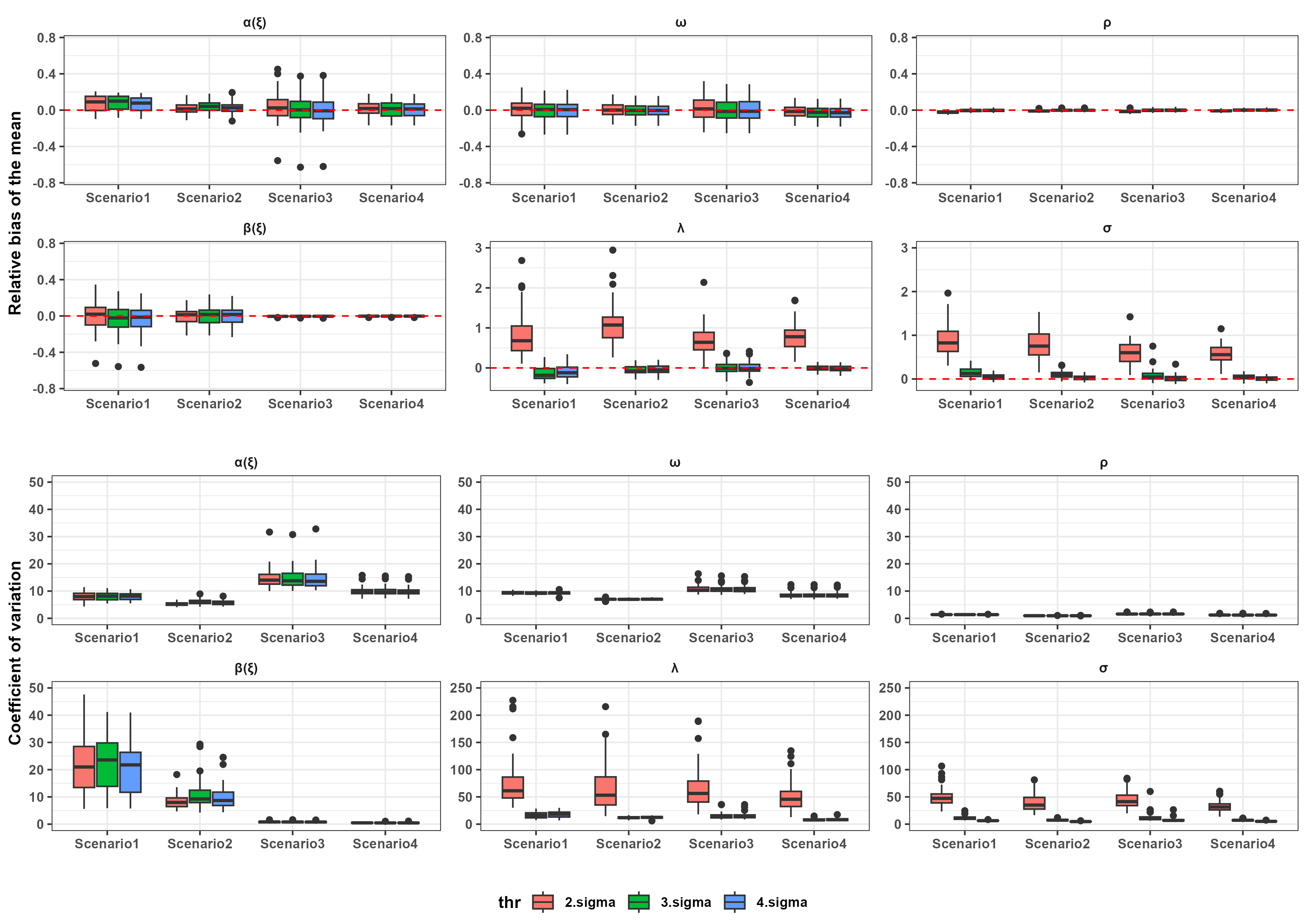
We simulated 50 datasets per scenario and fitted the dispersal-based occupancy model to each simulated dataset three times, with increasing values of . We used km, km and km for scenarios 1 and 3 and km, km and km for scenarios 2 and 4. This corresponded to , and ensuring comparable thresholds between scenarios. For all combinations of scenario and threshold, we computed parameters’ relative bias of the mean and coefficient of variation. We also evaluated the proportion of times the 95% credible interval contained the true value.
2.4 Case study 1: Wolf recolonization in France
We applied the model to wolf occurrence data collected in France by a network of trained professional and non-professional observers (Duchamp et al., 2011) between 1994 and 2016. The data was retrieved from (Louvrier et al., 2018) and comprises opportunistic records of scats and footprints monitored each year between December and March. We used the same design as in the original study, defining 10-by-10 km sites covering a large part of the country, 1-year primary occasions, and secondary occasions corresponding to each month of the monitoring period. In their analysis, the authors constructed a sampling effort variable based on the number of people registered in the monitoring network in the vicinity of each site (see details in Louvrier et al. (2018)). We set the detection probability to in sites where no sampling occurred and used sampling effort and road density to model detection probabilities. Wolves are known to occasionally disperse over very long distances (Ciucci et al., 2009), which can influence range dynamics in ways that our assumption of null dispersal beyond a threshold distance may fail to account for, potentially biasing inferences. To account for potential long distance dispersal we included a background dispersal pressure , and set . We set a prior to on the logit scale to force small values of ensuring that the effective dispersal pressure is unaffected near occupied areas, but keeping a small dispersal pressure and therefore a small colonization probability even far from colonization fronts. We modeled the installation probability as a function of five environmental variables: forest cover, farmland cover, mean altitude, proportion of high altitude, and distance to the closest barrier (highway or major river). See Table S1 for a complete description of all covariates.

2.5 Case study 2: Otter range expansion in France
For the second case study, we used a dataset of Eurasian otter occurrences across France between 2000 and 2023. Data was extracted from the Observatoire National des Mammifères data platform (ONM, https://observatoire-mammiferes.fr/) managed by the French Society for the Study and Protection of Mammals (SFEPM). This platform aggregates otter occurrence data in France collected by naturalist associations, nature users, or professional wildlife managers, and includes both standardized data (mostly based on the IUCN standard protocol (Reuther et al., 2000)) and opportunistic observations. We defined our sites as pixels in a 10-by-10 km grid covering the whole mainland France () to match the resolution at which otter monitoring is conducted across the country (Kuhn et al., 2019). To estimate yearly detection probability, we defined six 4-year primary occasions, treating each year as a secondary occasion, and assuming constant occupancy during these periods. Important heterogeneity in detection probability could arise from the fact that we included both opportunistic presence only data – prone to sampling biases (Backstrom et al., 2024) – and standardized data. To account for that, we included a survey variable indicating whether a standardized survey was conducted in a given site and year. For the period, it was defined by extracting negative records from the ONM platform, assuming that surveyed sites provided at least one non-detection during the year. Annual maps of standardized surveys were inspected by experts involved in otter monitoring in France to confirm that they provided reliable information of survey effort. For the period, we used the dataset compiled by (Lacombe et al., 2025), in which detection/non-detection data from 24 naturalist associations were consistently classified as standardized surveys or opportunistic observations. We included a linear time trend to account for temporal changes in sampling intensity, estimated separately for sites with and without standardized surveys.
To evaluate effects of the environment on range dynamics, we modeled the installation probability as a function of environmental variables representative of land use, water quality, landscape structure and human disturbances, which have been shown to affect otter presence in certain places. We did not include variables of resource availability as we assume that variation in abundance for different prey groups at a km² resolution would reflect broad ecological gradients rather than local resource limitation, which is more likely to operate at finer spatial scales. Specifically, we included the proportion of intensive agricultural area, heterogeneous agricultural area, and forest cover in a m buffer around rivers within each pixel; the diatom biological index of water quality; the cumulated river length and surface of water-bodies, and the terrain slope. See Table S1 for a complete description of all covariates.
2.6 Implementation in the Bayesian framework
Models were fitted within the Bayesian framework using Markov Chain Monte Carlo (MCMC). For all analyses, we used priors for the logit intercepts and slopes of , , and , and for and respectively. For the two case-studies we set the maximum dispersal distance to km and performed variable selection using the Reversible Jump MCMC algorithm (RJMCMC) (Green, 1995). This allows transitions between models including or not each covariate using latent indicator variables, enabling the estimation of inclusion probabilities for all covariates. We ran two MCMC chains with 2500 burn-in iterations and 2500 posterior samples per model in the simulation study and 10000 burn-in iterations and 5000 posterior samples for the two case studies. We assessed convergence for all model by visually inspecting trace plots and computing the Gelman-Rubin statistics (Brooks and Gelman, 1998). All analyses were conducted using R Version 4.4.2 (R Core Team, 2026) and Nimble (de Valpine et al., 2017).

3 Results
3.1 Simulation study
For , and , the credible interval of the relative bias overlapped zero for all scenarios, showing unbiased estimation (Fig. 2A). Parameter was slightly overestimated for scenario 1 (short dispersal distance, generalist species) with an estimated relative bias of 0.07 [-0.08, 0.19] (mean [95CI]), but unbiased for other scenarios. Parameters and were strongly biased when the model was fitted with with a relative bias of 0.85 [0.24, 2.05] and 0.71 [0.14, 1.40] respectively. This bias decreased markedly with increasing . For , bias was negligible when in all scenarios except the short-distance generalist case, where slight underestimation persisted even at (-0.10 [-0.36, 0.25]). For , unbiased estimation was achieved when for short dispersal distances and when for long dispersal distances.
Mean estimated coefficient of variation was consistently below 15% for , , and (Fig. 2B) showing good precision. Precision for was lower in short-distance scenarios, particularly for the short-distance generalist scenario (21.7 [7.62, 40.5]; 9.62 [4.89, 22.6] for scenarios 1 & 2, respectively) than for long-distance scenarios (0.81 [0.26, 1.49]; 0.50 [0.26, 0.87]). For and , the coefficient of variation was around 50% when , but decreased to under 20% when .
Overall, when all parameters were estimated with low bias and good coverage, with between 84% and 100% of all 95CIs containing the true parameter value (Fig. S3).
3.2 Case studies

In total, wolves were detected at 2004 1-year primary occasions, with a number of detections ranging from min. 2 sites in 1994 to max. 213 in 2015. When wolves were observed at a site, the average number of positive secondary occasions was 1.80 [1.76, 1.85]. Otters were detected at 9886 4-year primary occasions (min. 695 for 2000-2003, max. 2462 for 2020-2023), with an average number of years with a detection of 2.10 [2.08, 2.13] during positive primary occasions.
The two models converged, with for all parameters. All estimates are shown in Table S2. On average, wolves had a low monthly detection probability of 0.14 [0.13, 0.16]. Otter yearly detection probability was higher, reaching 0.72 [0.69, 0.74] where standardized surveys were conducted and 0.40 [0.40, 0.41] elsewhere (Fig. S4). Wolf detection probability was strongly affected by sampling effort and road density, increasing up to 0.69 [0.54, 0.75] where sampling was highest, and to 0.35 [0.32, 0.39] near roads. For otters, yearly detection probability did not vary over time in surveyed sites, but the opportunistic detection probability increased to 0.62 [0.61, 0.63] in 2023. Extinction probability was low for the two species, namely 0.27 [0.25, 0.29] for wolves and 0.14 [0.13, 0.15] for otters.
Wolves and otters had roughly similar dispersal kernels, with a scale parameters of 10.72 km [9.15, 12.4] for wolves and 12.26 km [11.4, 13.3] for otters, suggesting a maximum dispersal distance of c.a. 40 km every 4-years for otters and 35 km per year for wolves (Fig. 3). Wolves also had a background dispersal rate of 0.0065 [0.0040, 0.010], reflecting occasional long-distance colonization events. Average installation probability was significantly lower for wolves (0.18 [0.13, 0.26]) than for otters (0.87 [0.80, 0.92]). This resulted in strong differences in maps of installation probability: wolves had overall low installation probabilities, with higher values restricted to a few areas (e.g. Alps, Pyrenean mountains) while otters showed high installation probabilities in most of the study area that decreased in some places to intermediate values (Fig. 4). The RJMCMC algorithm identified several covariates affecting installation probability with high support (inclusion probability , Fig. S5). Altitude had a strong positive effects on wolf installation probability, while forest cover had a slighter positive effect and proportion of high-altitude a negative effect (Fig. 5A-C). Otter installation probability was primarily driven by a negative effect of intensive agricultural area, whereas urban areas and riparian vegetation had positive effects (Fig. 5D-F).
4 Discussion
In this study, we developed a process-based dynamic occupancy model to study the distribution of range expanding species. Our work addresses two key limitations that have so far prevented such models from being applied at large spatial scales. First, we introduced a flexible and ecologically interpretable formulation of the colonization process that allows to simultaneously capture species-specific dispersal patterns and effects of the environment, providing realistic insights into drivers of range dynamics under non-equilibrium conditions (Yackulic et al., 2015). Second, by introducing a computationally efficient approach, we addressed the computational burden associated with connectivity calculations, letting us apply the model to landscapes comprising over 5000 sites, extending the applicability of models initially developed for metapopulations to large-scale distribution studies.

In our simulation study, the model could reliably retrieve parameter values for most scenarios when the threshold distance was large enough (Fig. 2). Only for the generalist short-dispersal distance scenario, small biases remained in the posterior mean of the dispersal rate and the intercept of the installation probability , showing weak identifiability for these parameters under certain conditions. In that case, it is likely due to the short dispersal distances and high installation probability leading to a near-deterministic progression of the colonization front, causing partial redundancy between parameters. Despite this weak identifiability in specific contexts, we show in Appendix 1 that both parameters are necessary to maintain sufficient flexibility in the dispersal kernel across a broad range of ecological scenarios. This flexibility is critical because overly restrictive dispersal formulations can generate compensatory mechanisms, incorrectly attributing spatial structure to environmental covariates rather than dispersal processes, therefore affecting the model’s ability to disentangle effects of dispersal and environment.
Too small values of would truncate relevant spatial information leading to biased parameter estimates (Fig. 2). Based on our simulations, we recommend choosing to be at least three times the scale parameter of the dispersal process . As is unknown prior to model fitting, the adequacy of this threshold can only be assessed a posteriori, which we consider to be a necessary step before interpreting model estimates. For our case-studies, this assumption was largely met as was below 12.5 km in both cases.
Our two case-studies revealed contrasting colonization dynamics, despite similar estimated dispersal kernels for otters and wolves (Fig. 3). Wolf installation probability was heterogeneous and strongly affected by the environment (Fig. 4, Fig. 5A-C) leading to small and spatially fragmented populations in the Alps and other mountainous areas (Fig. 6). The effects of environmental variables were consistent with previous knowledge on this species. In particular, the effects of altitude, forest cover and proportion of high altitude (Fig. 5A-C) were similar from those reported in (Louvrier et al., 2018). The persistence of a strong altitude effect after explicitly accounting for dispersal suggests that it reflects an ecological association with mountainous habitats, rather than solely historical colonization patterns (Valière et al., 2003). This association may be driven by the lower human densities and higher densities of wild ungulates (Valière et al., 2003; Loison et al., 2003) in Alpine environments. Interestingly, Louvrier et al. (2018) found a slight effect of farmland cover that our model did not detect. This likely reflects differences in model structure, namely that our model simultaneously estimates dispersal pressure and occupancy states, creating a coupling that may reduce sensitivity to potential biases in detection or sampling effort that could otherwise induce spurious occupancy–environment relationships (Risk et al., 2011; Guillera-Arroita, 2017). By contrast, otter rapidly expanded in all directions resulting in a dense, largely contiguous distribution (Fig. 6). In agreement with previous studies, we found otter presence to be negatively associated with cropland surface (see for example Couturier et al. (2023)) and positively with riparian vegetation (Looy et al., 2014). More unexpectedly, we found a positive effects of urban areas. A similar pattern was detected in southern France by Couturier et al. (2023) and likely reflects a combined effect of high survey effort, relatively good quality of freshwater habitats in many peri-urban contexts and otters ability to thrive in heavily urbanized areas (Lacombe et al., 2026; Weinberger et al., 2016; Lee and Luan, 2025). Despite this overall consistency, our results diverged from previous studies in several aspects. For instance, we did not find any effects of aquatic habitats (but see Romanowski et al. (2013); Quinonez et al. (2018); Looy et al. (2014)) or water pollution (Couturier et al., 2023). More generally, although many studies reported strong habitat dependence (Romanowski et al., 2013; Loy et al., 2009), environmental effects appeared comparatively moderate in our case (Fig. 4), with a high and relatively homogeneous installation probability across the country. This suggests that, at least in France, part of the observed association between otter presence and environmental variables arises from dispersal history rather than habitat selection.
The model can be improved by incorporating more functional definitions of connectivity. Indeed, we defined connectivity as a function of Euclidean distance between sites. However, animal capacities to reach distant locations are influenced by their ability to move through complex landscapes (With, 2004). To capture this, Euclidean distance is often replaced in connectivity analyses by functional metrics like least-cost path (Coulon et al., 2015; Sutherland et al., 2015) or commute-time (McRae et al., 2008; Kervellec et al., 2024) distances, both relying on a representation of the landscape as a resistance surface. Integrating a resistance-based formulation of connectivity would be particularly relevant for species like the otter which primarily disperse along rivers and coastlines (Agostini et al., 2025) and where the configuration of watersheds could create functionally isolated habitats despite apparent geographical proximity. More broadly, dispersal is often constrained by anthropogenic or natural barriers that Euclidean distance alone cannot capture. For instance, highways and large rivers have been shown to limit distributions for many large carnivores (Kervellec et al., 2023; Bauduin et al., 2025). In the case of wolves, highways reduce movement rates and increase mortality (Alexander et al., 2005; Ciucci et al., 2009), potentially affecting range expansion patterns. Although our wolf model partly accounted for such barriers through their effects on installation probability, it did not capture how they affect connectivity. Incorporating functional metrics such as least-cost-path or commute-time distances would therefore represent a major improvement, allowing the model to explicitly assess how landscape features facilitate or impede dispersal. This would not only improve inference on the processes shaping species distributions, but also provide a powerful framework to evaluate how mitigation strategies, such as wildlife crossings, corridor restoration, or barrier removal, may restore connectivity and improve recolonization potential.
A limitation of our approach is that environmental effects are estimated only within the subset of accessible sites, i.e., sites the species can access given its estimated dispersal abilities. While this is consistent with the underlying process, it may limit the ability to infer habitat relationships across the full range of environmental conditions within the study area. In particular, because environmental gradients are only partially sampled, the model may fail to capture relationships that occur outside the range of observed conditions, including potential nonlinear responses. This limitation is illustrated by the effect of urbanization on otters, for which the model estimates a positive association, leading to high predicted installation probabilities in highly urbanized areas such as in and around Paris (Fig. 4). However, these areas are unlikely to be suitable for the species (Kuhn et al., 2019), suggesting that the relationship may change at higher levels of urbanization that are not well represented within the accessible portion of the landscape. More generally, this highlights that environmental effects inferred from dispersal-based models should be interpreted with caution, as they may reflect only a subset of the underlying ecological relationships.
To conclude, our model can be interpreted as a process-based null model of range dynamics, in which spatial patterns primarily emerge from species-specific dispersal processes, while environmental effects are estimated as deviations from this baseline. By explicitly disentangling the influence of dispersal and habitat selection, we show that species distributions can reflect fundamentally different dynamics, with some species primarily constrained by the environment and others by their dispersal abilities. These results highlight the need for caution when interpreting habitat–distribution relationships in non-equilibrium systems. In light of the increasing availability of large-scale and long-term biodiversity data and advances in occupancy modeling, our framework offers new opportunities to study range dynamics using mechanistic approaches across entire landscapes. Such approaches provide a promising framework to investigate the processes shaping species distributions under non-equilibrium conditions, while also offering practical tools for anticipating the spread of invasive species, supporting the recovery of threatened populations, and managing human–wildlife interactions.
Acknowledgements
This research benefited from discussions conducted within the DISCAR working group, funded by the French Foundation for Research on Biodiversity (FRB) through its synthesis center CESAB.
We would like to thank all volunteer and professional observers who participated in data collection by providing records of otter and wolf occurrence as part of the National Action Plan for the Eurasian Otter and the French Large Carnivore Network. We would also like to thank all regional coordinators involved in the Otter National Action Plan for organizing the standardized surveys in their regions and for sharing their datasets.
We received funding from the City of Montpellier and Montpellier Méditerranée Métropole through the partnership agreement with the Centre for Functional and Evolutionary Ecology, from the University of Montpellier through its Labex Cemeb, and from the Beauval Nature association. This research was partly funded by the ANR through the project nachos for “Interdisciplinary approach to small carnivores - humans relationships” (grant ANR-25-CE03-5469).
CRediT authorship contribution statement
Simon Lacombe: Conceptualization, Data curation, Formal analysis, Methodology, Visualization, Writing – original draft, Writing – review and editing. Sébastien Devillard: Conceptualization, Supervision, Writing – review and editing. Cécile Kauffmann: Data curation, Validation, Writing – review and editing. Olivier Gimenez: Conceptualization, Methodology, Supervision, Writing –- review and editing.
Declaration of Competing Interest
The authors declare that they have no known competing financial interests or personal relationships that could have appeared to influence the work reported in this paper.
Declaration of generative AI and AI-assisted technologies in the writing process
During the preparation of this work, the authors used ChatGPT to polish the text and enhance the English language. After using this tool, the authors reviewed and edited the content as needed and take full responsibility for the content of the published article.
Data availability statement
Codes and data are available at https://github.com/SimLacombe/PB-DOM.
References
- A non-invasive genetics insight into population structure and recolonization dynamics of the Eurasian otter (Lutra lutra) at the boundary of its Italian core range. Mammalian Biology (en). External Links: ISSN 1618-1476, Link, Document Cited by: §4.
- Traffic volume and highway permeability for a mammalian community in the Canadian Rocky Mountains. Canadian Geographer / Le géographe canadien 49 (4), pp. 321–331 (en). External Links: ISSN 1541-0064, Link, Document Cited by: §4.
- Estimating sampling biases in citizen science datasets. Ibis (en). External Links: ISSN 1474-919X, Link, Document Cited by: §2.5.
- Modelling Eurasian lynx populations in Western Europe: What prospects for the next 50 years?. Peer Community Journal 5 (en). External Links: ISSN 2804-3871, Link, Document Cited by: §4.
- Hierarchical modeling of an invasive spread: the Eurasian Collared-Dove Streptopelia decaocto in the United States. Ecological Applications 21 (1), pp. 290–302 (en). External Links: ISSN 1939-5582, Link, Document Cited by: §1.
- Dynamic occupancy models for explicit colonization processes. Ecology 97 (1), pp. 194–204 (en). External Links: ISSN 1939-9170, Link, Document Cited by: §1, §1.
- General Methods for Monitoring Convergence of Iterative Simulations. Journal of Computational and Graphical Statistics 7 (4), pp. 434–455. External Links: Link, Document Cited by: §2.6.
- Spatial occupancy models for predicting metapopulation dynamics and viability following reintroduction. Journal of Applied Ecology 52 (5), pp. 1325–1333 (en). External Links: ISSN 1365-2664, Link, Document Cited by: §1, §2.1.
- Long-Distance Dispersal of a Rescued Wolf From the Northern Apennines to the Western Alps. The Journal of Wildlife Management 73 (8), pp. 1300–1306 (en). External Links: ISSN 1937-2817, Link, Document Cited by: §2.4, §4.
- A stochastic movement simulator improves estimates of landscape connectivity. Ecology 96 (8), pp. 2203–2213 (en). External Links: ISSN 0012-9658, 1939-9170, Link, Document Cited by: §1, §4.
- Intensive agriculture as the main limiting factor of the otter’s return in southwest France. Biological Conservation 279, pp. 109927. External Links: ISSN 0006-3207, Link, Document Cited by: §4.
- Programming with models: writing statistical algorithms for general model structures with {NIMBLE}. Journal of Computational and Graphical Statistics 26 (2), pp. 403–417. External Links: Document Cited by: §2.6.
- Colonization and extinction dynamics of an annual plant metapopulation in an urban environment. Oikos 120 (8), pp. 1240–1246 (en). External Links: ISSN 1600-0706, Link, Document Cited by: §1, §1, §2.1.
- spOccupancy: An R package for single-species, multi-species, and integrated spatial occupancy models. Methods in Ecology and Evolution 13 (8), pp. 1670–1678 (en). External Links: ISSN 2041-210X, Link, Document Cited by: §1.
- Wolf monitoring in France : a dual frame process to survey time- and space-related changes in the population. Hystrix the Italian Journal of Mammalogy 23 (1), pp. 14–28 (english). External Links: ISSN 0394-1914, 1825-5272, Link, Document Cited by: §2.4.
- Integrated species distribution models reveal spatiotemporal patterns of human–wildlife conflict. Ecological Applications 32 (7), pp. e2647 (en). External Links: ISSN 1939-5582, Link, Document Cited by: §1.
- Ice age distributions of European small mammals: insights from species distribution modelling. Journal of Biogeography 36 (6), pp. 1152–1163 (en). External Links: ISSN 1365-2699, Link, Document Cited by: §1.
- Reversible jump Markov chain Monte Carlo computation and Bayesian model determination. Biometrika 82 (4), pp. 711–732. External Links: ISSN 0006-3444, Link, Document Cited by: §2.6.
- Effects of spatial autocorrelation and imperfect detection on species distribution models. Methods in Ecology and Evolution 9 (6), pp. 1614–1625 (en). External Links: ISSN 2041-210X, Link, Document Cited by: §1.
- Modelling of species distributions, range dynamics and communities under imperfect detection: advances, challenges and opportunities. Ecography 40 (2), pp. 281–295 (en). External Links: ISSN 1600-0587, Link, Document Cited by: §1, §1, §4.
- Predicting species distribution: Offering more than simple habitat models. Ecology Letters 8, pp. 993–1009. External Links: ISSN 1461-023X, Document Cited by: §1.
- Increasing connectivity between metapopulation ecology and landscape ecology. Ecology 99 (5), pp. 1119–1128 (en). External Links: ISSN 1939-9170, Link, Document Cited by: §1, §1.
- Bringing circuit theory into spatial occupancy models to assess landscape connectivity. Methods in Ecology and Evolution 15 (11), pp. 2141–2152 (en). External Links: ISSN 2041-210X, Link, Document Cited by: §1, §1, §2.1, §4.
- Integrating opportunistic and structured non-invasive surveys with spatial capture-recapture models to map connectivity of the Pyrenean brown bear population. Biological Conservation 278, pp. 109875. External Links: ISSN 0006-3207, Link, Document Cited by: §4.
- Plan national d’actions en faveur de la Loutre d’Europe (Lutra lutra) 2019-2028.. Technical report SFEPM and DREAL Nouvelle-Aquitaine, Poitiers. Cited by: §2.5, §4.
- Comparative efficiency of eDNA, camera traps and scat surveys to detect a semi-aquatic mammal across multiple catchments. bioRxiv (en). Note: ISSN: 2692-8205 Pages: 2026.04.28.721338 Section: New Results External Links: Link, Document Cited by: §4.
- Range expansion and reconnection of historical populations in the Eurasian otter (Lutra lutra) in France: Insights from heterogeneous data and integrated species distribution modelling. Biological Conservation 307, pp. 111179. External Links: ISSN 0006-3207, Link, Document Cited by: §2.5.
- Is my sdm good enough? insights from a citizen science dataset in a point process modeling framework. Ecological Modelling 438, pp. 109283. External Links: ISSN 0304-3800, Link, Document Cited by: §1.
- A Review on Eurasian Otters in Urban Areas: Principles for the Enhancement of Biodiversity. Diversity 17 (5), pp. 356 (en). External Links: ISSN 1424-2818, Link, Document Cited by: §4.
- Large Herbivores in European Alpine Ecosystems: Current Status and Challenges for the Future. In Alpine Biodiversity in Europe, L. Nagy, G. Grabherr, C. Körner, and D. B. A. Thompson (Eds.), pp. 351–366 (en). External Links: ISBN 978-3-642-18967-8, Link, Document Cited by: §4.
- Integrated modelling of functional and structural connectivity of river corridors for European otter recovery. Ecological Modelling 273, pp. p. 228 (en). External Links: Link, Document Cited by: §4.
- Mapping and explaining wolf recolonization in France using dynamic occupancy models and opportunistic data. Ecography 41 (4), pp. 647–660 (en). External Links: ISSN 09067590, Link, Document Cited by: §1, §1, §2.4, §4.
- Otter Lutra lutra population expansion: assessing habitat suitability and connectivity in southern Italy. Folia Zoologica 58 (3), pp. 309 (en). Cited by: §4.
- Lutra lutra (amended version of 2021 assessment). The IUCN Red List of Threatened Species 2022: e.T12419A218069689. External Links: Link Cited by: §1.
- Occupancy Estimation and Modeling: Inferring Patterns and Dynamics of Species Occurrence. Elsevier (en). External Links: ISBN 978-0-12-407245-9 Cited by: §1, §2.1.
- Using Circuit Theory to Model Connectivity in Ecology, Evolution, and Conservation. Ecology 89 (10), pp. 2712–2724 (en). External Links: ISSN 1939-9170, Link, Document Cited by: §4.
- A review of otter distribution modeling: Approach, scale, and metrics. IUCN/SCC Otter Specialist Group Bulletin 35, pp. 97–127. Cited by: §1, §4.
- R: A Language and Environment for Statistical Computing.. R Foundation for Statistical Computing, Vienna, Austria. External Links: Link Cited by: §2.6.
- Surveying and monitoring distribution and population trends of the Eurasian otter (Lutra lutra) : guidelines and evaluation of the standard method for surveys as recommended by the European section of the IUCN/SSC Otter Specialist Group. GN-Gruppe Naturschutz GmbH, DE (en). External Links: ISBN 978-3-927650-18-3, Link Cited by: §2.5.
- A robust-design formulation of the incidence function model of metapopulation dynamics applied to two species of rails. Ecology 92 (2), pp. 462–474 (en). External Links: ISSN 1939-9170, Link, Document Cited by: §4.
- Habitat correlates of the Eurasian otter Lutra lutra recolonizing Central Poland. Acta Theriologica 58 (2), pp. 149–155. External Links: ISSN 0001-7051, Link, Document Cited by: §4.
- Climate or migration: what limited European beech post-glacial colonization?. Global Ecology and Biogeography 22 (11), pp. 1217–1227 (en). External Links: ISSN 1466-8238, Link, Document Cited by: §1.
- A demographic, spatially explicit patch occupancy model of metapopulation dynamics and persistence. Ecology 95 (11), pp. 3149–3160 (en). External Links: ISSN 1939-9170, Link, Document Cited by: §1, §1, §2.1.
- Modelling non-Euclidean movement and landscape connectivity in highly structured ecological networks. Methods in Ecology and Evolution 6 (2), pp. 169–177 (en). External Links: ISSN 2041-210X, Link, Document Cited by: §4.
- Disentangling the contributions of dispersal limitation, ecological drift, and ecological filtering to wild bee community assembly. Ecosphere 8 (1), pp. e01650 (en). External Links: ISSN 2150-8925, Link, Document Cited by: §1.
- Long-distance wolf recolonization of France and Switzerland inferred from non-invasive genetic sampling over a period of 10 years. Animal Conservation 6 (1), pp. 83–92 (en). External Links: ISSN 1469-1795, Link, Document Cited by: §1, §4.
- Flexible habitat selection paves the way for a recovery of otter populations in the European Alps. Biological Conservation 199, pp. 88–95. External Links: ISSN 0006-3207, Link, Document Cited by: §4.
- Metapopulation Dynamics. Ecology, Genetics and Evolution of Metapopulations. External Links: Link, Document Cited by: §1, §4.
- To predict the niche, model colonization and extinction. Ecology 96 (1), pp. 16–23 (en). External Links: ISSN 1939-9170, Link, Document Cited by: §1, §1, §4.