Three dimensional, spherically polarized magnetic fields

We consider the special case $\theta=\theta(x)$, for which eqs. (3) are analytically integrable along characteristics. Integrating the second equation from $z=0$ with initial condition $\phi_{0}(x,y)$ and substituting into the first yields the characteristic curves $y(z)$:

In the equation above, we label each characteristic by its footpoint $y(0)=y_{0}$ and we define

The characteristics form a family of semicircles in the $(y,z)$ plane whose center and radii of curvature depend on the footpoint $y_{0}$. As a consequence, these curves eventually intersect, implying the formation of genuine discontinuities in $y$ at finite $z$ for fixed $x$. Alternatively, the solution becomes singular when $az+D=1$ before intersection occurs. In either case, smooth three-dimensional solutions with exactly constant $|{\bf B}|$ do exist over a finite interval in $z$, but discontinuities (or singularities) eventually develop. The extent of the interval where a smooth solution exists increases as $\theta^{\prime}(x)$ decreases, that is, as the amplitude of the field rotation becomes smaller or if it varies slowly.

When the phase $\theta=\theta(y)$, eqs. (3) can be combined, yielding

The characteristics are therefore determined by solving

The form of the right-hand-side of eq. (9) shows that the characteristic velocity depends on both $x$ and the footpoint $y_{0}$ through $\phi$. Consequently, neighboring characteristics generally propagate at different speeds, providing a mechanism for characteristics convergence and eventual intersection. For $z\ll 1$, the characteristics are approximated to lowest order by $y(z)\simeq y_{0}-z/\tan(\phi_{0}(y_{0},x))$. Because intersections occur when $dy/dy_{0}=0$, an estimate for the crossing distance is $z_{c}\simeq-\sin^{2}\phi_{0}/\phi_{0}^{\prime}$. If $\phi_{0}^{\prime}=0$, the dominant linear term vanishes and a higher order expansion is necessary. Expanding eq. (9) to the next non-vanishing order shows that neighboring characteristics start to converge when $\theta^{\prime\prime}\cot\theta-(\theta^{\prime})^{2}\csc^{2}\theta>0$ with an estimated $z_{c}\simeq\pm\sqrt{(2(\sin\phi_{0})^{2})/(\theta^{\prime\prime}\cot\theta-(\theta^{\prime})^{2}\csc^{2}\theta})$. Since $\theta$ and $\phi_{0}$ are oscillatory within the hemisphere, they necessarily contain regions where neighboring characteristics are compressive. The estimates above therefore predict finite crossing distance $z_{c}$, indicating that intersection of characteristics is generically expected. As an example, we construct a field rotation reproducing a switchback by choosing

in the range $-L_{x}/2\leq x\leq L_{x}/2$, $-L_{y}/2\leq y\leq L_{y}/2$ with $L_{x}=L_{y}=2\pi$. Figure 1 shows a family of characteristics for this system at $x=1$ that converge and intersect at $y\simeq\pm 1$ and $z\simeq 1.7$ where the solution breaks down. As in case 1, the extent of the domain of existence becomes larger for smaller amplitude fluctuations.

The magnetic field shown in Fig. 2 was reconstructed after integration of eq. (2). Achieving good numerical accuracy in this integration (with $\nabla\cdot\mathbf{B}\ll 1$ numerically) becomes increasingly challenging as the phase $\phi$, and hence $\mathbf{B}$, steepens. However, the method of characteristics informs on the domain in which regular solutions exist, ensuring that the numerical solution is physically correct despite increasing numerical errors on the divergence. The integration was therefore performed on a domain $L_{x}\times L_{y}\times L_{z}=2\pi\times 2\pi\times 1.69$ using $128\times 512\times 256$ mesh points with a pseudospectral filter in the $y$ direction to prevent numerical instabilities as the steepening develops.

The resulting unperturbed field is primarily along $x$, ${\bf B}=(0.86,0.5,,0)$, with rms fluctuations $\delta B_{x}=0.47$, $\delta B_{y}=0.18$, and $\delta B_{z}=0.23$. A developing discontinuity at $y\simeq\pm 1$ is apparent in the contour plot of $B_{z}$ at the plane $z=1.69$ (Fig. 2, top panel), and is accompanied by a sharp deflection of $B_{y}$ at the same location. The resulting field lines are shown in the full 3D domain in Fig. 2, bottom panel. This explicit example illustrates that switchbacks do not need to exhibit sharp boundaries everywhere a field reversal exists, although discontinuities eventually develop. Additionally, a consequence of our construction method is that while the switchback can be localized in the $(x,y)$ plane, it necessarily extends in the third ($z$) direction. Thus, consistent with the analytic results of Shi et al. (2024), our example indicates that a switchback can be fully bounded in three dimensions only if the constant-$|\bf{B}|$ condition is relaxed.

We build a broadband spectrum starting from a random superposition of scale-independent rotations:

where we have used the first 5 modes in each direction and $\varphi_{i}$ are random phases. We then renormalize the extrema of $\theta$ and $\phi_{0}$ to prescribe the desired angular coverage of the field, which controls the amplitude of magnetic fluctuations. The dependence of $\theta$ on $z$ now modifies the behavior of characteristics discussed in previous paragraphs, and a general conclusion on existence of smooth solutions cannot be drawn. Nevertheless, due to the nonlinear and oscillatory behavior of $F$, it is expected that discontinuities form at some $z$ for generic phase functions. As in the previous cases, we empirically find that the admissible range of domain sizes $L_{z}$ expands as the fluctuation amplitude decreases, or if wavelengths increase.

The phases defined in eq. (12)-(13) produce angle distributions that are approximately Gaussian and centered near the midpoint of the imposed range. Consequently, large deflections with $\theta>\pi/2$ lack the intermittent character typical of solar‑wind switchbacks. To generate sparse large‑amplitude deflections in $B_{x}$, we apply an exponential mapping to produce a skewed distribution:

where $\theta_{0}$ sets the smallest value of $\theta$, and $\beta$ and $\alpha$ control the skewness and variance. In the case-study shown here we chose $\theta_{0}=0.1$, $\alpha=5$ and $\beta=0.1$. We integrated eq. (2) in a domain $L_{x}=L_{y}=2\pi$ and $L_{z}=0.3$ using $128\times 512\times 256$ mesh points.

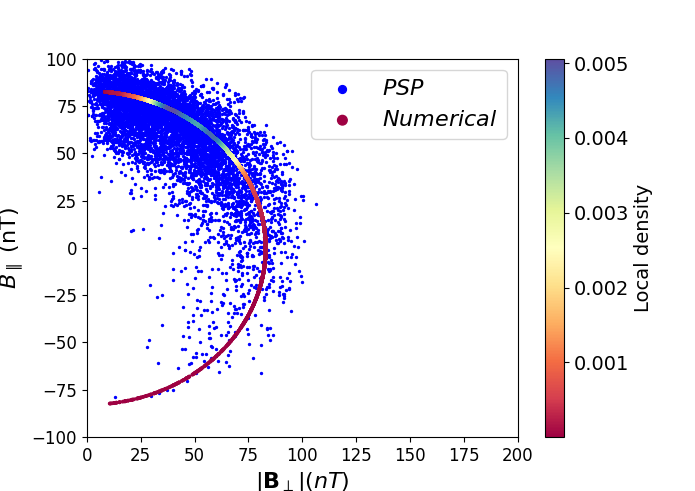
The reconstructed magnetic field has a mean $\langle{\bf B}\rangle=(0.75,0.57,-0.006)$ and rms amplitudes $\delta B_{x}=0.2$, $\delta B_{y}=0.18$ and $\delta B_{z}=0.178$ with embedded switchbacks. The largest deflection is reached at ${\bf x}=(1.13,2.12,0.0355)$ where $B_{x}=-0.99$. Fig. 3, top panel, shows the magnetic field at $z=0.0355$, where a switchback can be seen near the top right corner of the plot. The bottom panel shows the 1D reduced spectrum of the resulting field as a function of the perpendicular and parallel wave number, $k_{\perp}$ and $|k_{\parallel}|$, defined with respect to the mean field. The resulting spectrum is steeper than observed, scaling approximately as $k_{\perp}^{-3}$ and $|k_{\parallel}|^{-6}$, although it displays an anisotropic distribution with energy mostly in $k_{\perp}$ as in the solar wind (Dasso et al., 2005; Horbury et al., 2012; Sioulas et al., 2023). We note that we tested different initial conditions with weighted Fourier coefficients and by increasing the number of modes, and we found that the resulting magnetic spectra remain largely unaffected.

For the sake of illustration, Fig. 4 presents a comparison between the numerical solution and PSP data at 1 minute resolution during the first perihelion (from 11-4-2018 to 11-7-2018, at an average distance $R=0.18$ au). The top panel shows the distribution of the deflection parameter $\mathcal{Z}=1/2(1-\cos\Theta)$ (Dudok de Wit et al., 2020), where $\Theta$ is the angle between the local total magnetic field and the mean field over the integration domain (or over 12 hours for PSP). The middle panel compares the scatter plot of $B_{x}$ vs. the perpendicular components $|{\bf B_{\perp}}|$ with PSP data (for which we show $-B_{r}$ on the $y$-axis), after rescaling the numerical solution to 83 nT. The color code shown in the side bar indicates the density of numerical points. The bottom panel shows a 1d cut of $|{\bf B}|$ and $B_{x}$ at $x=1.13$ and $z=0.0355$ that we compare with a sub-interval of PSP, again after rescaling the numerical solution in amplitude and converting the $y$-axis to the same time interval length of PSP. Fig. 4 shows that the numerical field reproduces essential patterns in the observations: a wide distribution of field deflections including switchbacks ($\mathcal{Z}>0.5$), with the most probable state at a small angle to the radial direction while undergoing sparse deflections at larger angles. However, our solution displays less frequent extreme events and exhibits a smoother profile due to the limited number of modes initialized. Increasing the values of $\alpha$ and $\beta$ and the number of modes could improve the agreement, but stronger tails and smaller scale fluctuations tend to rapidly produce stiff solutions. This suggests that a flatter distribution of ${\mathcal{Z}}$ might be favored by relaxing the constant-$|{\bf B}|$ constraint.