A Provably Convergent and Practical Algorithm for Gromov–Wasserstein Optimal Transport
Abstract
Gromov–Wasserstein optimal transport (GWOT) aligns metric measure spaces by matching their within-domain relational structures, but large-scale GWOT remains challenging because its objective is nonconvex and projection onto the transport polytope is often solved only approximately in practice. This leads to a gap between practical projected-gradient implementations and convergence theory, which typically assumes exact projections. For squared-loss GWOT, we propose an inexact projected-gradient framework with a verifiable feasibility-residual-based inexact condition for the projection subproblem. This condition is directly computable and avoids unknown quantities such as the exact projection point. Under this implementable condition, we prove subsequential convergence to stationary points and, with a mild tolerance-decay condition, convergence of the whole sequence. The resulting method retains the simplicity and sparsity of projected-gradient schemes while providing rigorous convergence guarantees, turning projected-gradient methods into a principled and scalable approach for GWOT with provable reliability.
1 Introduction
Let and be two metric measure spaces equipped with probability vectors and , where and denote the all-ones vectors of dimensions and , respectively. Given intra-domain dissimilarity matrices and with, e.g., and , Gromov–Wasserstein optimal transport (GWOT) seeks a soft coupling that aligns the relational structures of the two spaces Mémoli (2011). Unlike classical OT Villani (2009), which relies on a cross-domain cost between and , GWOT compares within-domain relations. It searches for a coupling , under which pairs in are matched, in aggregate, with pairs in having similar dissimilarity. This makes GWOT particularly useful when the two domains live in incomparable feature spaces and only their internal metric structures are meaningful. As a result, GWOT has found applications in, e.g., geometry matching and analysis Mémoli (2011); Peyré et al. (2016), graph matching and network alignment Xu et al. (2019), heterogeneous domain adaptation Yan et al. (2018), and single-cell multi-omics alignment Demetci et al. (2020).
Define the transport polytope . Given a loss function , the GWOT problem is given as follows:
| (1.1) |
The objective is generally nonconvex due to the bilinear terms . In this work, we focus on the squared loss , for which the objective admits the decomposition
Therefore, problem (1.1) is equivalent to
| (1.2) |
where is -smooth with . We highlight that, although we present the analysis for squared-loss GWOT, the proposed framework applies more broadly to GWOT-type problems with Lipschitz-smooth losses, including the fused GWOT Ma et al. (2023).
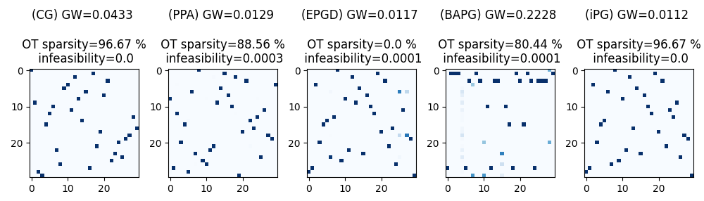
Given the structure of problem (1.2), (Euclidean) projected gradient (PG) methods are among the simplest first-order schemes for solving it: each iteration takes a gradient step and then projects onto the transport polytope. This gives a natural non-entropic approach that preserves the sparse structure expected from solutions of unregularized GWOT problems. In practice, however, exact Euclidean projection onto can be expensive at scale. Implementations therefore often compute the projection only approximately, using an inner iterative solver with a heuristic stopping rule. This creates a gap between practical PG implementations and standard convergence theory, which typically assumes that each projection step is solved exactly. It also helps explain why much recent work on large-scale GWOT has focused on single-loop first-order methods; see, e.g., Li et al. (2023) and the references therein. By avoiding an inner projection, such methods sidestep the need to specify how accurately the projection subproblem should be solved.
Nevertheless, this leaves open an essential question: can the simple PG framework be made both practical and rigorous when the projection is computed only approximately? We answer this question affirmatively. The key idea is to replace the exact projection requirement with a verifiable inexact condition for the projection subproblem. This condition is formulated by the primal feasibility residual associated with the dual iterate, and is therefore directly computable during the inner solve. In particular, it avoids unknown quantities such as the exact projection point. Under this implementable condition, we establish rigorous convergence guarantees for the resulting inexact PG iterates. Consequently, the proposed PG framework retains its simplicity, sparsity, and scalability while admitting a convergence theory that reflects how the method is truly implemented in practice. Figure 1 illustrates the performance of our method compared with representative GWOT solvers.
Contributions.
Our contributions in this work are summarized as follows.
-
•
An inexact PG framework with a simple verifiable inexact condition. We develop an inexact PG (iPG) method for GWOT in which the projection onto the transport polytope is solved only approximately. The inexact condition is constructed from the primal feasibility residual associated with the dual iterate, making it directly computable during the inner solve while avoiding inaccessible quantities such as the exact projection point.
-
•
Convergence guarantees under inexact computations. We prove subsequential convergence of the generated inexact iterates to stationary points of the GWOT problem under summable projection errors. We further establish convergence of the whole sequence under an additional mild tolerance-decay condition. These results align the theory with practical implementations.
-
•
Empirical validation on graph alignment. We evaluate the proposed method on graph-alignment tasks and compare it with representative GWOT solvers. The results show that iPG produces sparse and nearly feasible transport plans while maintaining competitive objective values, alignment accuracy, and runtime.
1.1 Related Work
Computational optimal transport.
Optimal transport (OT) provides a geometric framework for comparing probability measures through a cost-minimizing mass transportation problem. In the classical Monge formulation, one seeks a deterministic transport map, which is often difficult to compute. The Kantorovich relaxation instead optimizes over transport plans (couplings), leading to a linear programming problem that forms the foundation of modern OT theory and computation Kantorovich (2006). In data science, computational OT Peyré and Cuturi (2019) has been driven largely by entropic regularization, which smooths the Kantorovich problem and reduces it to a matrix-scaling problem solvable by Sinkhorn iterations. This has enabled fast and differentiable approximations of Wasserstein-type distances Cuturi (2013). Recent advances in entropic OT have improved scalability through stochastic and semi-discrete or continuous dual methods that require only sampling access to distributions Genevay et al. (2016), faster algorithms with explicit complexity guarantees such as Greenkhorn and near-linear-time approximation methods Altschuler et al. (2017), and high-dimensional approximations including low-rank formulations Scetbon et al. (2021) and projection-based approaches such as sliced OT Bonneel et al. (2015). Beyond entropic methods, which generally provide approximate OT solutions, a growing body of work has focused on computing exact OT solutions using splitting methods Liang et al. (2024); Lu and Yang (2024); Yang et al. (2021); Zhang et al. (2025), entropic proximal point methods Chu et al. (2023); Wu et al. (2025); Xie et al. (2020); Yang and Toh (2022), augmented Lagrangian methods Li et al. (2020); Yang et al. (2024); Zhu et al. (2024), and Newton-type methods Hou et al. (2024); Liu et al. (2022). These algorithmic advances have further expanded the impact of OT in machine learning, with fruitful applications as mentioned earlier.
Algorithmic frameworks for GWOT.
Algorithmic developments for GWOT can be broadly grouped into several lines. A classical and still widely used approach is conditional-gradient (CG) (a.k.a., Frank–Wolfe-type Frank and Wolfe (1956)) optimization, which repeatedly linearizes the nonconvex quadratic GW objective over the transport polytope and solves OT-type subproblems, leading to simple iterations but often relatively slow convergence Vayer et al. (2019). A second major line relies on entropic regularization, where the entropic projected gradient descent (EPGD) method combines gradient steps with Sinkhorn-type projections and has become a foundational computational approach for approximate GWOT Peyré et al. (2016). Related proximal regularization ideas were further developed in the entropic proximal point algorithm (PPA), which solves a sequence of better-conditioned regularized GW subproblems and improves numerical stability Xu et al. (2019). Beyond these basic first-order schemes, several scalable variants have been proposed for graph matching and partitioning. A representative example is the S-GWL framework, which exploits multi-scale and recursive strategies to extend GW-based matching to larger graphs Xu et al. (2019). More recent work has pursued stronger algorithmic simplifications, broader modeling variants, and sharper guarantees. The Bregman alternating projected gradient (BAPG) method gives a provable single-loop first-order scheme for a relaxed GW formulation Li et al. (2023). Semi-relaxed and unbalanced GW formulations enlarge the modeling scope and lead to more flexible algorithms for graphs and measures with mass variation or outliers Séjourné et al. (2021); Vincent-Cuaz et al. (2022). Low-rank methods can dramatically reduce computational complexity and yield near-linear or linear-time approximations in favorable regimes Scetbon et al. (2022), while semidefinite relaxations provide a complementary direction aimed at stronger lower bounds and, in some cases, certificates of global optimality beyond local stationarity Chen et al. (2024). In this landscape, our practical inexact Euclidean projected-gradient method belongs to the class of non-entropic first-order methods. Its distinguishing feature is that it works directly over the original transport polytope while allowing the projection subproblem to be solved only approximately under a simple and verifiable inexact condition.
Notation.
We use () and () to denote the sets of -dimensional real (non-negative) vectors and real (non-negative) matrices, respectively. For a vector , and denote its and norms, respectively. For a matrix , and denote its spectral and Frobenius norms, respectively, and we write . For a proper closed convex function and a scalar , the -subdifferential of at is defined by . When , reduces to the classical convex subdifferential . For a closed convex set , its indicator function is denoted by , where if and otherwise. We use to denote the Euclidean projection of onto , and to denote the distance from to , i.e., .
2 A Provably Convergent Inexact Projected Gradient Framework
For simplicity, we denote the linear mapping and the vector as , and The adjoint mapping of is denoted as . In this section, building on the classical projected-gradient (PG) framework for solving the GWOT problem (1.2), we develop a novel practical inexact projected gradient (iPG) method. Our key contribution is a novel feasibility-residual-based inexact condition that is simple to check in practice and truly implementable, avoiding unknown quantities and hard-to-verify requirements, yet still yields strong convergence guarantees comparable to those of the exact PG method. The complete algorithmic framework is presented in Algorithm 1.
Input: Let be a sequence of nonnegative scalars satisfying , and let be the inverse learning rate.
Choose arbitrarily.
Set .
while a termination criterion is not met, do
-
Step 1.
Find a vector such that the matrix
(2.1) is an approximate solution of the projection subproblem
(2.2) satisfying the following inexact condition:
(2.3) -
Step 2.
Set and go to Step 1.
end while
Output:
Well-definiteness of Algorithm 1.
We first show that the algorithm is well-defined. Specifically, fix any and any prescribed tolerance . We claim that there always exists a dual vector such that
| (2.4) |
To justify (2.4), consider the dual formulation of the projection subproblem (2.3), which is the unconstrained convex minimization problem
| (2.5) |
A direct calculation gives . Let be any minimizer of (2.5). By the first-order optimality condition, we have that and the associated primal solution is , which is the (unique) optimal solution of the primal projection subproblem (2.2). Moreover, since is convex and continuously differentiable, problem (2.5) can be solved by standard algorithms for smooth convex optimization, such as accelerated gradient methods Beck and Teboulle (2009); Nesterov (1983) or Newton-type methods Liang et al. (2021); Yang et al. (2023); Zhao et al. (2010). In particular, one can apply a convergent inner solver to generate a sequence satisfying as for some minimizer . By the continuity of and the optimality condition , we obtain
Consequently, if , there exists an inner iteration index large enough such that satisfies (2.4); if , one may take . Thus, the inexact condition (2.3) is attainable at every outer iteration , and Algorithm 1 is well defined.
Remark 2.1 (Comments on scaling by in (2.3)).
The factor is included to make (2.3) robust to potentially large dual iterates. In general, without additional regularity assumptions, there is no guarantee that the sequence remains uniformly bounded. Since the analysis involves products between the dual iterate and the primal feasibility residual, the normalization ensures that these products remain controlled even when is large. At the same time, the condition still forces the primal feasibility residual to vanish as .
We next analyze the convergence behavior of the proposed algorithm. We first establish subsequential convergence to stationary points and then prove full sequential convergence of the whole sequence. Proofs of all theoretical results are deferred to the Appendices. For notational convenience, let and . These two quantities are used only in the analysis and are not needed in practical implementations.
Theorem 2.1.
Suppose that . Let be the sequence generated by Algorithm 1. Then, there exists a shadow sequence satisfying and such that the following statements hold.
-
1.
(Boundedness) Both sequences and are bounded;
-
2.
(Approximate sufficient descent property) For any , it holds that
(2.6) where ;
-
3.
(Shared accumulation points) The limit exists, and . Moreover, any accumulation point of is an accumulation point of , and vice versa;
-
4.
(Subsequential convergence) Any accumulation point of or is a stationary point of the GWOT problem (1.2), i.e., . Moreover, for any accumulation point of or .
Theorem 2.1 establishes subsequential convergence by constructing a feasible shadow sequence close to the possibly infeasible iterates . This is sufficient for proving that all accumulation points are stationary. However, to prove convergence of the whole sequence, one needs a stronger mechanism: a descent sequence that is compatible with the projected gradient geometry and the Kurdyka–Łojasiewicz (KL) framework (see Attouch et al. (2013); Bolte et al. (2007, 2014b) for more details). The auxiliary sequence is not uniquely defined and is not generated by the exact projected gradient step, so it is not the most convenient object for a full sequential convergence argument.
For this reason, we introduce a second shadow sequence, namely, the exact projection points
| (2.7) |
The sequence plays the role of the ideal exact PG iterate. If the computed inexact iterate can be controlled relative to , then the implementable residual condition can be converted into an approximate sufficient descent property for . This is the key ingredient needed to combine the inexact PG recursion with the KL property and establish full sequential convergence.
The following proposition provides precisely this bridge. It shows that the primal feasibility residual controls the distance from the computed inexact projection to the exact projection , uniformly in .
Proposition 2.1 (Error bound for the inexact projection step).
Theorem 2.2.
Let be generated by Algorithm 1, and let be defined by (2.7). Then,
-
1.
(Approximate sufficient descent property) For any , it holds that
- 2.
-
3.
(Full sequential convergence) Let be an arbitrary rational constant. Suppose that the tolerance parameter sequence is chosen such that
(2.8) Then, the whole sequence converges to a stationary point of the GWOT problem (1.2).
Remark 2.2 (A simple choice of ).
Let . To ensure (2.8), one can set with and . Indeed, follows from , and Thus, whenever . Equivalently, , whose right-hand side decreases to as . Hence, by taking sufficiently large, one may choose a decay exponent only slightly larger than in practice, as in our numerical experiments.
3 Numerical Experiments on Graph Alignment via GWOT
In this section, we evaluate the proposed iPG on a graph alignment task and compare it with several representative GWOT solvers. The goal is to assess how well different algorithms balance objective quality, computational efficiency, feasibility, and sparsity, and alignment accuracy.
Graph alignment problem and GWOT formulation.
Graph alignment Xu et al. (2019) aims to identify correspondences between the node sets of two graphs that represent the same or similar underlying relational structure. Let be two undirected graphs with and . Here, we assume that the two graphs are from a common latent graph up to a hidden permutation, possibly with additional structural perturbations. The goal is to recover the unknown node matching between and .
A key difficulty in graph alignment is that node labels are arbitrary, so direct comparison of adjacency matrices is not meaningful. Instead, one compares the intrinsic geometry of the two graphs. To this end, for each graph we construct an intra-graph cost matrix , where and encode pairwise shortest-path distances between nodes within each graph.111Without loss of generality, we assume that both graphs are connected. These matrices summarize the internal metric structure of the graphs and are invariant to relabeling. Given node mass distributions , the graph alignment problem can be relaxed into a GWOT problem. In our experiments, we use the standard squared loss and set . The transport matrix obtained from solving the GWOT then plays the role of a soft matching between the node sets of the two graphs: a large value of indicates that node is strongly associated with node with the hope that a good coupling should map pairs of nodes in to pairs of nodes in with similar relational distances. Therefore, even when node identities are completely scrambled, the GWOT objective may recover alignment information purely from structural consistency.
Graph generation.
We generate graph alignment instances as follows. First, we sample a connected Erdős–Rényi graph222Using the function networkx.erdos_renyi_graph at: https://networkx.org/documentation/stable/reference/generated/networkx.generators.random_graphs.erdos_renyi_graph.html with nodes and edge probability . If a sampled graph is disconnected, we resample until a connected graph is obtained. Let denote the adjacency matrix of . Next, we generate a random hidden permutation over and construct a permuted copy of by where is the permutation matrix associated with . This produces a graph that is isomorphic to but with relabeled nodes. To make the alignment problem nontrivial, we then inject structural noise into the second graph by independently flipping each off-diagonal edge with probability . More precisely, for each unordered pair with , the edge indicator is replaced by its complement with probability , while symmetry and a zero diagonal are preserved. If the resulting noisy graph is disconnected, we regenerate the noise until a connected graph is obtained. The final graph is denoted by . For each graph, we compute the all-pairs shortest-path distance matrix and normalize it by its maximum entry These normalized distance matrices are used as inputs to the GWOT solvers. Since is generated from a permuted version of before noise is added, the hidden permutation provides the ground-truth node correspondence. This enables us to evaluate the quality of the recovered alignment quantitatively.
Baseline methods.
We consider 20 independently generated instances using the 20 random seeds for each problem size. All reported statistics are averaged over these 20 runs. We compare the proposed iPG with the following GWOT solvers implemented in the open-source POT package333https://pythonot.github.io/.
-
•
CG: the standard conditional-gradient GW solver. 444Implemented in ot.gromov.gromov_wasserstein.
-
•
PPA: the entropic GW solver with the proximal point algorithm backend. 555Implemented in ot.gromov.entropic_gromov_wasserstein with solver="PPA".
-
•
EPGD: the entropic GW solver with projected gradient descent backend. 666Implemented in ot.gromov.entropic_gromov_wasserstein with solver="PGD".
-
•
BAPG: the Bregman alternating projected gradient method. 777Implemented ot.gromov.BAPG_gromov_wasserstein.
-
•
iPG: the proposed inexact projected gradient method.
All methods are applied to the same normalized shortest-path matrices and uniform marginals with the same initialization . For each returned coupling , we record the final GW loss reported by the solver. This measures the quality of the structural alignment in terms of the optimization objective. Lower values indicate better agreement between the relational geometries of the two graphs. To evaluate how well the computed coupling satisfies the transport constraints, we use the residual . Smaller values indicate better feasibility with respect to the prescribed marginals. Since exact optimal transport solutions are often sparse, it is informative to examine the sparsity pattern of the returned coupling. We measure sparsity as the fraction of zero entries . A higher sparsity score indicates a more concentrated transport plan. To evaluate alignment quality relative to the ground truth, we convert the soft coupling into a hard permutation-like assignment using the Hungarian algorithm 888Implemented in scipy.optimize.linear_sum_assignment at: https://docs.scipy.org/doc/scipy/reference/generated/scipy.optimize.linear_sum_assignment.html, and then compare it with the true permutation matrix via .
Solver hyperparameters.
For the CG solver, we set the maximum number of outer iterations to . For the entropic solvers PPA, EPGD, and BAPG, we test four entropic regularization levels . Each solver is run with a maximum of iterations. This allows us to examine the effect of entropy strength on objective value, feasibility, sparsity, and runtime. For the proposed iPG method, we terminate the algorithm when the maximum iterations or the relative successive change is less than . The projection subproblems are solved by the accelerated gradient method Beck and Teboulle (2009) with , . Runs that terminate with an exception are marked as failures and excluded from the statistical averages, while the number of successful and failed runs is tracked separately.

(a) Loss

(b) Sparsity

(c) Feasibility

(d) Accuracy

(e) Time
Computational results.
The computational results are summarized in Figure 2; detailed numerical records can be found in Appendix D. Overall, the proposed iPG method delivers the strongest balance among GW objective value, sparsity, feasibility, alignment accuracy, and runtime across the tested instances. In particular, iPG consistently attains one of the smallest losses among all methods while maintaining extremely small feasibility residuals. At the same time, it returns couplings with sparsity essentially equal to one, which is much closer to the expected structure of an exact transport solution than the couplings produced by the entropic baselines. This structural advantage is important in graph alignment, since a sparse and nearly feasible coupling is substantially easier to interpret and to round into a high-quality discrete correspondence. Consistent with this, iPG achieves the best overall alignment accuracy and remains competitive in runtime as the problem size increases.
The comparisons also clarify the strengths and weaknesses of the competing approaches. The classical CG method always produces very sparse and exactly feasible couplings, but its loss and matching accuracy are generally inferior to those of other methods, suggesting that feasibility and sparsity alone do not guarantee a good alignment if the method converges to a poorer stationary point. EPGD is computationally cheap and achieves very small feasibility residuals for moderate and large values of the entropic parameter, but its iterates remain essentially dense across all problem sizes, which is undesirable for recovering a discrete matching. More broadly, the entropic PG-type approach does not preserve the sparse structure that one expects from the unregularized GWOT solution, and feasibility can also become problematic when the regularization is small. PPA is more competitive in terms of loss and accuracy, and for some values of , it performs similarly to iPG; however, it is clearly sensitive to the choice of , returns noticeably denser couplings than iPG, and becomes substantially slower as increases. BAPG is the least robust among the tested methods: it fails when is small, and even when it succeeds, its feasibility and alignment accuracy are often unsatisfactory unless the regularization is tuned carefully.
Taken together, these results support the central message of the paper. A non-entropic projected-gradient framework with practical inexact projections can preserve the expected structural features of unregularized GWOT solutions, in particular near-feasibility and high sparsity, while remaining computationally efficient. In contrast, entropic methods often introduce a smoothing bias that yields denser couplings and may weaken downstream matching performance, whereas exact-feasibility methods such as CG can converge to less favorable stationary points in terms of objective value and alignment accuracy. Overall, the proposed iPG method offers a robust, scalable, and structurally faithful approach to graph alignment via GWOT.
4 Conclusions
In this paper, we developed a provably convergent inexact projected gradient framework for solving the GWOT problem, with a particular emphasis on practical implementability with convergence guarantees. Our main contribution is a truly verifiable inexact condition for the approximate projection step onto the transport polytope, which avoids unknown quantities, admits a simple feasibility-residual-based stopping rule, and helps bridge the gap between scalable implementations and rigorous convergence theory. Under this implementable condition, we established subsequential convergence to stationary points and, under an additional mild tolerance-decay condition, convergence of the whole sequence. Numerical experiments on graph alignment further show that the proposed iPG method achieves a favorable balance among objective quality, sparsity, feasibility, alignment accuracy, and computational efficiency, compared with several representative GWOT solvers.
Looking ahead, several limitations of the current work merit further investigation. On the application side, it will be important to deploy the proposed framework in more real-world GWOT tasks, such as network alignment, shape analysis, biological data integration, and cross-domain representation matching. On the computational side, an important next step is to develop high-performance implementations that better exploit modern hardware architectures, including multi-core CPUs, GPUs, and distributed systems, so as to further enhance scalability for large-scale problems. It is also of strong interest to design stochastic and mini-batch variants of the proposed method possibly with variance reduction techniques, which may provide additional efficiency gains in massive data settings and open the door to online or streaming GWOT computations.
References
- [1] (2017) Near-linear time approximation algorithms for optimal transport via Sinkhorn iteration. In Advances in Neural Information Processing Systems, Cited by: Appendix A, §1.1.
- [2] (2010) Proximal alternating minimization and projection methods for nonconvex problems: An approach based on the Kurdyka-Łojasiewicz inequality. Mathematics of Operations Research 35 (2), pp. 438–457. Cited by: Appendix C.
- [3] (2013) Convergence of descent methods for semi-algebraic and tame problems: proximal algorithms, forward–backward splitting, and regularized Gauss–Seidel methods. Mathematical Programming 137 (1), pp. 91–129. Cited by: Appendix C, Appendix C, §2.
- [4] (2009) A fast iterative shrinkage-thresholding algorithm for linear inverse problems. SIAM Journal on Imaging Sciences 2 (1), pp. 183–202. Cited by: §2, §3.
- [5] (2007) The Łojasiewicz inequality for nonsmooth subanalytic functions with applications to subgradient dynamical systems. SIAM Journal on Optimization 17 (4), pp. 1205–1223. Cited by: Appendix C, §2.
- [6] (2014) Proximal alternating linearized minimization for nonconvex and nonsmooth problems. Mathematical Programming 146 (1), pp. 459–494. Cited by: Appendix C.
- [7] (2014) Proximal alternating linearized minimization for nonconvex and nonsmooth problems. Mathematical Programming 146 (1), pp. 459–494. Cited by: Appendix C, §2.
- [8] (2015) Sliced and Radon Wasserstein barycenters of measures. Journal of Mathematical Imaging and Vision 51 (1), pp. 22–45. Cited by: §1.1.
- [9] (2024) Semidefinite relaxations of the Gromov–Wasserstein distance. In Advances in Neural Information Processing Systems, Cited by: §1.1.
- [10] (2023) An efficient implementable inexact entropic proximal point algorithm for a class of linear programming problems. Computational Optimization and Applications 85 (1), pp. 107–146. Cited by: §1.1.
- [11] (2013) Sinkhorn distances: Lightspeed computation of optimal transport. In Advances in Neural Information Processing Systems, Cited by: §1.1.
- [12] (2020) Gromov–Wasserstein optimal transport to align single-cell multi-omics data. bioRxiv. Cited by: §1.
- [13] (1956) An algorithm for quadratic programming. Naval Research Logistics Quarterly 3 (1–2), pp. 95–110. Cited by: §1.1.
- [14] (2016) Stochastic optimization for large-scale optimal transport. In Advances in Neural Information Processing Systems, Cited by: §1.1.
- [15] (1993) Convex analysis and minimization algorithms II: Advanced theory and bundle methods. Springer. Cited by: Appendix A.
- [16] (1952) On approximate solutions of systems of linear inequalities. Journal of Research of the National Bureau of Standards 49 (4), pp. 263–265. Cited by: Appendix B.
- [17] (2024) A sparse smoothing Newton method for solving discrete optimal transport problems. ACM Transactions on Mathematical Software 50 (3), pp. 1–26. Cited by: §1.1.
- [18] (2006) On the translocation of masses. Journal of Mathematical Sciences 133 (4). Cited by: §1.1.
- [19] (2023) A convergent single-loop algorithm for relaxation of Gromov–Wasserstein in graph data. In International Conference on Learning Representations, Cited by: Figure 1, Figure 1, §1.1, §1.
- [20] (2020) An asymptotically superlinearly convergent semismooth Newton augmented Lagrangian method for linear programming. SIAM Journal on Optimization 30 (3), pp. 2410–2440. Cited by: §1.1.
- [21] (2024) Accelerating multi-block constrained optimization through learning to optimize. arXiv preprint arXiv:2409.17320. Cited by: §1.1.
- [22] (2021) An inexact augmented Lagrangian method for second-order cone programming with applications. SIAM Journal on Optimization 31 (3), pp. 1748–1773. Cited by: §2.
- [23] (2022) A multiscale semi-smooth Newton method for optimal transport. Journal of Scientific Computing 91 (2), pp. 39. Cited by: §1.1.
- [24] (2024) PDOT: A practical primal-dual algorithm and a GPU-based solver for optimal transport. arXiv preprint arXiv:2407.19689. Cited by: §1.1.
- [25] (2023) Fused Gromov–Wasserstein graph mixup for graph-level classifications. In Advances in Neural Information Processing Systems, Cited by: §1.
- [26] (2011) Gromov–Wasserstein distances and the metric approach to object matching. Foundations of Computational Mathematics 11 (4), pp. 417–487. Cited by: §1.
- [27] (1983) A method of solving a convex programming problem with convergence rate . Soviet Mathematics Doklady 27 (2), pp. 372–376. Cited by: §2.
- [28] (2016) Gromov–Wasserstein averaging of kernel and distance matrices. In International Conference on Machine Learning, Cited by: Figure 1, Figure 1, §1.1, §1.
- [29] (2019) Computational optimal transport: With applications to data science. Now Foundations and Trends. Cited by: §1.1.
- [30] (1987) Introduction to optimization. Optimization Software Inc., New York. Cited by: Appendix A, Appendix C.
- [31] (1998) Variational analysis. Springer. Cited by: Appendix C, Appendix C.
- [32] (2021) Low-rank Sinkhorn factorization. In International Conference on Machine Learning, Cited by: §1.1.
- [33] (2022) Linear-time Gromov–Wasserstein distances using low rank couplings and costs. In International Conference on Machine Learning, Cited by: §1.1.
- [34] (2021) The unbalanced Gromov–Wasserstein distance: Conic formulation and relaxation. In Advances in Neural Information Processing Systems, Cited by: §1.1.
- [35] (2019) Optimal transport for structured data with application on graphs. In International Conference on Machine Learning, Cited by: Figure 1, Figure 1, §1.1.
- [36] (2009) Optimal transport: old and new. Vol. 338, Springer. Cited by: §1.
- [37] (2022) Semi-relaxed Gromov–Wasserstein divergence and applications on graphs. In International Conference on Learning Representations, Cited by: §1.1.
- [38] (2025) PINS: Proximal iterations with sparse Newton and Sinkhorn for optimal transport. arXiv preprint arXiv:2502.03749. Cited by: §1.1.
- [39] (2020) A fast proximal point method for computing exact Wasserstein distance. In Uncertainty in Artificial Intelligence, Cited by: §1.1.
- [40] (2019) Gromov–Wasserstein learning for graph matching and node embedding. In International Conference on Machine Learning, Cited by: Figure 1, Figure 1, §1.1, §1, §3.
- [41] (2018) Semi-supervised optimal transport for heterogeneous domain adaptation. In International Joint Conference on Artificial Intelligence, Cited by: §1.
- [42] (2023) An inexact projected gradient method with rounding and lifting by nonlinear programming for solving rank-one semidefinite relaxation of polynomial optimization. Mathematical Programming 201 (1), pp. 409–472. Cited by: §2.
- [43] (2021) A fast globally linearly convergent algorithm for the computation of Wasserstein barycenters. Journal of Machine Learning Research 22 (21), pp. 1–37. Cited by: §1.1.
- [44] (2024) A corrected inexact proximal augmented Lagrangian method with a relative error criterion for a class of group-quadratic regularized optimal transport problems. Journal of Scientific Computing 99 (3), pp. 79. Cited by: §1.1.
- [45] (2022) Bregman proximal point algorithm revisited: A new inexact version and its inertial variant. SIAM Journal on Optimization 32 (3), pp. 1523–1554. Cited by: §1.1.
- [46] (2025) HOT: An efficient Halpern accelerating algorithm for optimal transport problems. IEEE Transactions on Pattern Analysis and Machine Intelligence 47 (8), pp. 6703–6714. Cited by: §1.1.
- [47] (2010) A Newton-CG augmented Lagrangian method for semidefinite programming. SIAM Journal on Optimization 20 (4), pp. 1737–1765. Cited by: §2.
- [48] (2024) ripALM: A relative-type inexact proximal augmented Lagrangian method for linearly constrained convex optimization. arXiv preprint arXiv:2411.13267. Cited by: §1.1.
Appendix A Proof of Theorem 2.1
In this section, we provide a detailed proof for the subsequential convergence of Algorithm 1.
Lemma A.1 (Explicit error bound for when ).
Let and satisfy . For any , there exists such that
Proof.
The proof is straightforward with the second inequality following from [1, Lemma 7].
Note that the point constructed in Lemma A.1 need not coincide with the Euclidean projection of onto the feasible set .
Proof of Theorem 2.1.
The existence of the sequence follows from Lemma A.1.
Statement 1. The boundedness of follows from the boundedness of the feasible set . In particular, for all . Moreover, by the construction of , the definition of , and the inexact condition (2.3), we have that
where and . Thus, is also bounded.
Statement 2. Define
It is easy to verify that , (by the construction of in (2.1)), and
Moreover, by Statement 1, , and with , we have
Then, for any , we see that
where the third equality follows from , the first inequality follows from and , the second inequality follows from the construction of , and the third inequality follows from the inexact condition (2.3). This implies that is an -subdifferential of at the point . By taking in the above inequality, we obtain that
Since is -smooth, we have that
which leads to
This then implies (2.6) by setting .
Statement 3. It follows from (2.6) that
Since , one can verify that . Moreover, since is compact and is continuous, is bounded below on . Then, we can conclude that is convergent, i.e., the limit exists; see, e.g., [30, Section 2.2]. From (2.6) and the continuity of , we further see that
as . This, together with , proves that
Finally, since , we then obtain that any accumulation point of is an accumulation point of , and vice versa.
Statement 4. We only need to show that any accumulation point of is a stationary point of the GWOT problem (1.2). Since is bounded (by Statement 1), it has at least one accumulation point. Suppose that is an accumulation point and is a convergent subsequence such that . Since , we see that and from Statement 3 that
| (A.1) | ||||
as . Recall that is an -subdifferential of at , i.e.,
Then, passing to the limit in above relation and invoking (A.1), the Lipschitz continuity of , and the outer semicontinuity of (see, for example, [15, Proposition 4.1.1]) with (due to ), we see that
which implies that is a stationary point of the GWOT problem (1.2).
Finally, pick two arbitrary accumulation points and associated with the subsequences and , respectively. By the continuity of the function and the fact that is convergent, we see that . Hence, we conclude that is constant on the set of accumulation points and complete the proof.
Appendix B Proof of Proposition 2.1
Lemma B.1 (Uniform Hoffman error bound for projection).
For each , consider the projection problem
Let denote its unique solution. Then, there exists a constant , independent of all , such that for every and
one has
Proof.
For simplicity, we vectorize matrices and write the transport constraints in the form
where and is the matrix representation of . Similarly, let . Then, the projection problem is equivalent to
Its KKT system can be written as
or equivalently, there exists such that
Define the solution set of the KKT system by
Since the primal projection problem is strongly convex, every point in has the same primal component, namely, .
We now use the polyhedral structure. Note that the complementarity condition is a finite union of polyhedral systems. More precisely, for each index set , consider the polyhedral regime
On each such regime, the KKT system (if nonempty) becomes a linear system of equalities and inequalities whose coefficient matrices are independent of ; only the right-hand side depends affinely on . Hoffman’s error bound [16] for linear equalities and inequalities therefore gives a constant , depending only on the corresponding coefficient matrix, such that the distance to the solution set of this regime is bounded by the residual of the regime. Because there are only finitely many index sets , we can take
This constant is independent of .
Now, fix . Then, for any , set
By the projection property, there exists such that
Hence, this triple satisfies every KKT condition except possibly the affine feasibility equation . Therefore, the Hoffman error bound yields
Since every point in has primal component , we have
Returning to matrix notation gives
This completes the proof.
Proof of Proposition 2.1:
Appendix C Proof of Theorem 2.2
In this section, we establish the full sequential convergence. We first recall some standard notions in variational analysis. Let be a real finite dimensional Euclidean space equipped with an inner product and its induced norm . For a proper closed function , we write if and . The limiting subdifferential [31, Definition 8.3] of at is defined by
where denotes the Fréchet subdifferential. Specifically, if
When is continuously differentiable or convex, this limiting subdifferential reduces to the classical gradient or convex subdifferential, respectively; see [31, Exercise 8.8 and Proposition 8.12].
We next recall the Kurdyka-Łojasiewicz (KL) property (see [3, 5, 7] for more details), which is now a standard technical condition for establishing the convergence of the whole sequence in the nonconvex setting. For simplicity, let () denote a class of concave functions satisfying: (i) ; (ii) is continuously differentiable on and continuous at ; (iii) for all . The KL property is described as follows.
Definition C.1 (KL property).
Let be a proper closed function. We say that satisfies the Kurdyka-Łojasiewicz (KL) property at if there exist , a neighborhood of , and a function such that
for all . The function is called a KL function if it satisfies the KL property at every point of .
We also recall the uniformized KL property, which was established in [6, Lemma 6].
Proposition C.1 (Uniformized KL property).
Let be a proper closed function, and let be a compact set. Suppose that on for some constant and that satisfies the KL property at each point of . Then there exist , , and such that
for all .
Let be an arbitrary rational constant. The subsequent analysis makes use of the following auxiliary merit function:
| (C.1) |
Since is a nonempty polytope, is quadratic, and is rational, the function is proper, closed, and semialgebraic. Hence satisfies the KL property; see, e.g., [2, 3].
Proof of Theorem 2.2:
Statement 1. From the definition of in (2.7) and the first-order optimality condition of the projection problem, we have that
| (C.2) |
Then, there exists a such that
By the definition of the subdifferential of the indicator function , the following inequality holds for any feasible :
Also, by the -smoothness of , we see that
which implies that, for any ,
Now, let in the above, together with Proposition 2.1 and , we see that
for all .
Statement 2. Since the feasible set is bounded, the sequence is bounded. Moreover, since is compact and is continuous, is bounded below on . From Statement 1 and , we see that
This, together with (due to ), implies that is convergent; see e.g., [30, Section 2.2]. This, together with the inequality in Statement 1, further implies that . Consequently, and have the same set of accumulation points. By Theorem 2.1, and also share the same accumulation points, and thus the three sequences have the same set of accumulation points. Using these facts, we further have that , where is the constant given in Theorem 2.1.
Statement 3. In view of , we only need to show that the sequence is convergent. From Statement 1, by rearranging terms, dropping the term involving and denoting , we see that
Recall the definition of in (C.1) and set for . We see that
| (C.3) |
This implies that the sequence is non-increasing for and it is bounded from below due to the convergence of . Since as (due to ), we also have that
Without loss of generality, we assume that for all (otherwise, remains the same for all sufficiently large ).
From Statement 2, we see that for any accumulation point of the sequence , denoted as , where must be an accumulation point of the sequence , it must hold that . Denote as the set of accumulation point of , which is nonempty and compact. Since is a KL function, it then follows from the uniformized KL property (see Proposition C.1) that there exist , and such that
for all satisfying and . On the other hand, since and is non-increasing, then for such and , there exist such that and . Consequently, it holds that
We next derive an upper bound of . First, it follows from (C.2) that
Moreover, by Proposition 2.1, we have
Note that, for any ,
This implies that
Now, we denote
Since is concave and is non-increasing and converges to , we see that
where the last inequality follows from (C.3). Combining this with the KL inequality and the upper bound of derived previously, we see that
Taking the square root of both sides of the above gives
which leads to
Summing the above relation from to , we have
This, together with and , implies that
Hence, is a Cauchy sequence and therefore converges. Since , the whole sequence converges to the same limit, which is a stationary point of the GWOT problem (1.2). This completes the proof.
Appendix D Detailed Computational Results
| Method | Loss | Sparsity | Feasibility | Accuracy | Time | |
|---|---|---|---|---|---|---|
| BAPG | - | - | - | - | - | |
| 5.97e-01 | 0.83 | 8.03e-01 | 0.01 | 0.02 | ||
| 3.10e-02 | 0.48 | 2.27e-02 | 0.12 | 0.50 | ||
| 3.05e-02 | 0.00 | 1.46e-03 | 0.25 | 0.58 | ||
| CG | - | 3.60e-02 | 0.99 | 0.00e+00 | 0.02 | 0.00 |
| EPGD | 3.11e-02 | 0.00 | 5.54e-05 | 0.21 | 0.38 | |
| 5.35e-02 | 0.00 | 5.85e-17 | 0.06 | 0.00 | ||
| 5.36e-02 | 0.00 | 5.83e-17 | 0.04 | 0.00 | ||
| 5.36e-02 | 0.00 | 5.76e-17 | 0.04 | 0.00 | ||
| PPA | 3.53e-02 | 0.97 | 4.69e-05 | 0.10 | 1.83 | |
| 3.08e-02 | 0.43 | 1.04e-05 | 0.25 | 2.61 | ||
| 3.07e-02 | 0.01 | 1.52e-06 | 0.25 | 15.27 | ||
| 3.07e-02 | 0.00 | 1.92e-07 | 0.24 | 38.57 | ||
| iPG | - | 3.21e-02 | 0.99 | 7.63e-09 | 0.17 | 0.92 |
| Method | Loss | Sparsity | Feasibility | Accuracy | Time | |
|---|---|---|---|---|---|---|
| BAPG | - | - | - | - | - | |
| 8.05e-01 | 0.96 | 7.18e-01 | 0.01 | 0.21 | ||
| 1.06e-01 | 0.23 | 4.19e-03 | 0.67 | 0.91 | ||
| 1.10e-01 | 0.00 | 5.18e-04 | 0.55 | 1.64 | ||
| CG | - | 1.26e-01 | 0.99 | 0.00e+00 | 0.01 | 0.02 |
| EPGD | 1.11e-01 | 0.00 | 3.25e-05 | 0.51 | 0.49 | |
| 1.43e-01 | 0.00 | 5.04e-17 | 0.03 | 0.01 | ||
| 1.43e-01 | 0.00 | 4.82e-17 | 0.03 | 0.01 | ||
| 1.43e-01 | 0.00 | 5.01e-17 | 0.02 | 0.01 | ||
| PPA | 1.16e-01 | 0.84 | 5.10e-05 | 0.39 | 3.77 | |
| 1.12e-01 | 0.53 | 1.50e-05 | 0.51 | 8.97 | ||
| 1.10e-01 | 0.02 | 2.48e-06 | 0.55 | 22.54 | ||
| 1.10e-01 | 0.00 | 2.67e-07 | 0.55 | 37.65 | ||
| iPG | - | 1.13e-01 | 0.99 | 1.34e-09 | 0.46 | 5.63 |
| Method | Loss | Sparsity | Feasibility | Accuracy | Time | |
|---|---|---|---|---|---|---|
| BAPG | - | - | - | - | - | |
| 1.14e+00 | 0.98 | 7.48e-01 | 0.00 | 0.53 | ||
| 6.03e-02 | 0.29 | 6.15e-03 | 0.51 | 3.68 | ||
| 6.09e-02 | 0.00 | 5.35e-04 | 0.52 | 4.70 | ||
| CG | - | 8.34e-02 | 1.00 | 0.00e+00 | 0.01 | 0.05 |
| EPGD | 6.07e-02 | 0.00 | 1.85e-05 | 0.51 | 6.18 | |
| 1.03e-01 | 0.00 | 4.50e-17 | 0.02 | 0.01 | ||
| 1.03e-01 | 0.00 | 4.52e-17 | 0.02 | 0.01 | ||
| 1.03e-01 | 0.00 | 4.44e-17 | 0.02 | 0.01 | ||
| PPA | 6.65e-02 | 0.87 | 3.07e-05 | 0.43 | 5.39 | |
| 6.10e-02 | 0.49 | 6.25e-06 | 0.52 | 13.11 | ||
| 6.32e-02 | 0.02 | 1.09e-06 | 0.48 | 23.05 | ||
| 6.33e-02 | 0.00 | 1.28e-07 | 0.48 | 56.78 | ||
| iPG | - | 5.85e-02 | 1.00 | 1.15e-09 | 0.57 | 15.66 |
| Method | Loss | Sparsity | Feasibility | Accuracy | Time | |
|---|---|---|---|---|---|---|
| BAPG | - | - | - | - | - | |
| 1.16e+00 | 0.99 | 7.15e-01 | 0.00 | 1.82 | ||
| 4.40e-02 | 0.21 | 4.05e-03 | 0.62 | 5.69 | ||
| 4.41e-02 | 0.00 | 4.17e-04 | 0.65 | 8.28 | ||
| CG | - | 7.40e-02 | 1.00 | 0.00e+00 | 0.00 | 0.12 |
| EPGD | 4.44e-02 | 0.00 | 1.14e-05 | 0.62 | 8.37 | |
| 9.26e-02 | 0.00 | 4.66e-17 | 0.02 | 0.03 | ||
| 9.26e-02 | 0.00 | 4.69e-17 | 0.01 | 0.03 | ||
| 9.26e-02 | 0.00 | 4.60e-17 | 0.01 | 0.03 | ||
| PPA | 4.63e-02 | 0.79 | 1.40e-04 | 0.63 | 4.89 | |
| 4.44e-02 | 0.39 | 4.21e-06 | 0.64 | 13.13 | ||
| 4.43e-02 | 0.01 | 6.74e-07 | 0.64 | 39.81 | ||
| 4.47e-02 | 0.00 | 1.17e-07 | 0.63 | 68.51 | ||
| iPG | - | 3.95e-02 | 1.00 | 1.44e-09 | 0.71 | 31.89 |
| Method | Loss | Sparsity | Feasibility | Accuracy | Time | |
|---|---|---|---|---|---|---|
| BAPG | - | - | - | - | - | |
| 9.09e-01 | 0.99 | 5.86e-01 | 0.00 | 7.45 | ||
| 4.71e-02 | 0.20 | 3.62e-03 | 0.57 | 12.33 | ||
| 5.01e-02 | 0.00 | 4.38e-04 | 0.52 | 18.35 | ||
| CG | - | 7.52e-02 | 1.00 | 0.00e+00 | 0.00 | 0.21 |
| EPGD | 5.66e-02 | 0.00 | 1.59e-05 | 0.36 | 2.24 | |
| 9.19e-02 | 0.00 | 4.04e-17 | 0.01 | 0.05 | ||
| 9.19e-02 | 0.00 | 4.22e-17 | 0.01 | 0.05 | ||
| 9.19e-02 | 0.00 | 4.08e-17 | 0.01 | 0.05 | ||
| PPA | 4.52e-02 | 0.76 | 3.68e-05 | 0.62 | 10.46 | |
| 4.76e-02 | 0.45 | 3.78e-06 | 0.57 | 30.32 | ||
| 5.00e-02 | 0.01 | 6.57e-07 | 0.52 | 71.51 | ||
| 5.31e-02 | 0.00 | 8.47e-08 | 0.48 | 100.31 | ||
| iPG | - | 3.25e-02 | 1.00 | 9.26e-10 | 0.85 | 38.41 |