Conformalized Percentile Interval: Finite Sample Validity and Improved Conditional Performance
Abstract
Conformal prediction provides distribution-free predictive intervals with finite-sample marginal coverage. However, achieving conditional validity and interval efficiency (in terms of short interval length) remains challenging, particularly in complex settings with heteroskedasticity, skewed responses, or estimation errors. We propose a method that leverages the conditional cumulative distribution function (CDF) estimated via neural networks for a conformal-style calibration on responses transformed via the probability integral transform (PIT) to construct a finite-sample-adjusted percentile interval with the shortest length determined by the estimated conditional CDF. Calibrating in PIT space is effective because PIT values are asymptotically feature-independent when the CDF estimator is accurate, which mitigates feature-dependent miscoverage and improves conditional calibration. On the other hand, our percentile calibration adapts to the empirical PIT distribution, which is robust against a possibly imperfect estimation of the conditional CDF. We prove the finite-sample marginal coverage property of the proposed method and show its asymptotic conditional coverage under mild consistency conditions. Experiments on diverse synthetic and real-world benchmarks demonstrate better conditional calibration and substantially shorter intervals than existing methods.
1 Introduction
Reliable uncertainty quantification (UQ) is increasingly important as machine learning systems are deployed in high-stakes settings. While many classical UQ methods provide asymptotic guarantees or rely on strong distributional assumptions [13, 22], real-world applications demand finite-sample validity that remains reliable under complex data and model misspecification. Conformal prediction provides a compelling solution: it can be wrapped around any predictive model (including modern deep networks and ensemble methods) and, without assumptions beyond data exchangeability, yields prediction sets with finite-sample marginal coverage [26, 14]. Specifically, given any pre-trained predictive model and a calibration dataset , where ’s are covariates and ’s are corresponding responses, conformal prediction learns a prediction-set function with a user-specified target coverage level , where is typically a small value, e.g., . For a new test point with covariate , it constructs a prediction set for the corresponding response such that
The marginal coverage guarantee provided by standard conformal prediction holds only on average over all possible test points. It may be insufficient for many high-stakes applications that require stronger reliability guarantees conditioned on specific test instances or subpopulations. For such applications, one may seek prediction sets that satisfy test-conditional coverage:
However, it has been shown that achieving exact test-conditional coverage while maintaining informative prediction sets is impossible in a fully distribution-free setting [7]. For practical purposes, one may instead relax this requirement to hold in an asymptotic sense and aim to improve conditional performance as much as possible. This forms the central objective of this work.
Achieving test-conditional coverage is substantially more challenging than marginal coverage. For example, standard residual-based conformal intervals rely on a global residual distribution, which can lead to feature-dependent miscoverage when the residual law varies across the feature space. To mitigate this, several methods have focused on designing adaptive conformity scores. A simple approach is to use variance-rescaled residual scores [14], which adjust for heteroskedasticity by normalizing residuals with an estimate of local variability. Going beyond scale adjustment, Conformalized Quantile Regression (CQR) [21] incorporates conditional quantile information to better capture heterogeneity in the response. To further incorporate richer distributional information, several distribution-aware methods have been proposed, including conditional histogram regression [23] and Distributional Conformal Prediction (DCP) [5]. Among these, DCP is most closely related to our work, as it also leverages conditional CDF estimation and performs calibration in the Probability Integral Transform (PIT) space. If the conditional CDF is estimated accurately, then the transformed variable should lie on the unit interval and be approximately uniformly distributed, with reduced dependence on the covariates. However, existing CDF-based approaches typically rely on a single conformity score in the PIT space, which may impose structural constraints (e.g., symmetry) and limit their ability to adapt to asymmetric errors.
Building on these ideas, we propose the Conformalized Percentile Interval (CPI). CPI performs endpoint calibration rather than score calibration, directly adjusting the lower and upper percentile bounds independently without any symmetry restriction. Specifically, using PIT values computed on a hold-out calibration set, we select lower and upper PIT cutoffs, and , as independent order statistics of the calibration PIT values. For a new feature vector , the adjusted percentile interval is constructed as
This approach adapts to the local distributional shape while retaining finite-sample marginal validity. In principle, our framework is flexible and can be paired with any conditional CDF estimator. In this work, we adopt the neural network conditional distribution estimator of Hu and Nan [11] for our experiments to demonstrate the practical performance of our framework and provide a concrete, specific implementation.
Our main contributions are:
-
•
A Novel PIT-Based Framework: We move beyond classic conformity scores to propose an adjusted percentile interval that directly calibrates percentile endpoints. The method is straightforward to implement, provides finite-sample marginal guarantees, and is compatible with any conditional CDF estimator.
-
•
Improved Conditional Coverage and Shorter Intervals: By leveraging conditional distribution estimation, CPI better captures local distributional shape, leading to improved and more stable conditional coverage. This improved alignment with the conditional distribution also results in shorter prediction intervals, particularly in settings with heteroskedasticity or asymmetric noise.
-
•
Robustness to Asymmetric Estimation Errors: Unlike existing CDF-based methods, which rely on a single conformity score in the PIT space and often impose symmetry, CPI independently calibrates upper and lower PIT cutoffs. This flexibility makes the framework robust to asymmetric estimation errors—common in cases of model misspecification or distribution shift—resulting in substantially shorter intervals without sacrificing coverage.
1.1 Related Work
A separate line of work improves local adaptivity by modifying the calibration procedure itself, for example by reweighting calibration points using neighborhood information around the test point [25, 9, 10, 17, 18, 8]. These approaches are also useful for improving subgroup-conditional performance or handling covariate shift. Efficiency in terms of interval width is another important aspect of prediction sets. A better fitted model typically leads to smaller prediction errors and thus narrower intervals [4, 24]. Efficiency is also closely related to conditional coverage: adaptive conformity scores, such as those in Lei et al. [14], Romano et al. [21], generally produce smaller prediction sets by accounting for heterogeneity in the data. In addition, ensemble strategies that improve either the predictive model or the conformity score during pretraining or calibration have been shown to further enhance efficiency [27, 28, 15]. Finally, the Predictability, Computability, and Stability (PCS) framework for uncertainty quantification [30, 1] combines model selection or augmentation with bootstrap-style perturbations to achieve strong empirical efficiency. These approaches are largely orthogonal to our framework and can potentially be combined with CPI to further improve conditional performance and efficiency.
2 Conformalized Percentile Interval (CPI)
We consider the same data-splitting setup as in split conformal prediction, which consists of three independent parts: a training set for CDF estimation; a calibration set with observations for finite-sample correction; and a test point with covariate . Our goal is to construct a prediction set for the response with a target coverage level of , .
Let denote the true conditional CDF of given . A percentile interval of the form
achieves the target coverage level for any starting point , provided the conditional CDF is known. In this section, we construct a conformalized percentile interval by first forming an adjusted interval in the PIT space—serving as a finite-sample correction to the nominal interval —using an estimated CDF and the calibration set. Finally, we map this adjusted interval back to the original response scale.
As mentioned earlier, the training step can be replaced by any pre-trained conditional distribution estimator. In the experiment, we focus specifically on the neural network conditional distribution estimator proposed by Hu and Nan [11], which we refer to as the NN-CDE model, and train it on . We show that it performs well within our procedure, making the overall approach practical and easy to implement in real-world settings. We use to denote the resulting estimate of the true conditional CDF , and to denote the corresponding conditional quantile function for .
2.1 General Framework
In general, the starting point for the nominal interval can be an arbitrary function, provided it is constructed independently of the calibration set. For example, could be a fixed constant, e.g. , or a pre-trained function derived solely from the training data that depends on the test covariate . We will discuss the length-optimal choice of later. The calibration procedure is detailed below and illustrated in Figure 1.

Step 1: Compute PIT values.
On the calibration set , compute the PIT values
and let denote the corresponding order statistics (with randomized tie-breaking when necessary).
If the estimated CDF were equal to the true conditional CDF, then the PIT values (as well as ) would follow a distribution. In that case, the PIT interval would be valid, and mapping it back via would yield a percentile interval with conditional coverage . However, because is estimated, the PIT values are not exactly uniform. Following the idea of conformal prediction [26], we therefore use the calibration set to better approximate the distribution of the PIT values.
Step 2: Select lower and upper PIT cutoffs.
Define the rank indices
and set the following PIT cutoff values from :
Then the adjusted PIT interval is , which serves as a finite-sample correction to from the empirical distribution of the PIT values.
Step 3: Invert the conditional CDF to form a prediction interval.
The final prediction set for the response is a percentile interval based on the calibrated PIT cutoffs obtained in Step 2. Specifically, given a new covariate value , we output the prediction interval
Thus, the resulting interval can be interpreted as a percentile interval with a finite-sample adjustment to the nominal interval . This adjustment corrects for the estimation error by calibrating the estimated conditional CDF in PIT space, resulting in prediction intervals with reliable finite-sample marginal coverage.
2.2 Length-optimal Choice of
CPI can be viewed as a percentile interval with a finite-sample adjustment applied to the nominal interval . While fixing serves as a solid basic method, from an efficiency perspective, we prefer intervals that capture the regions where the conditional distribution is most concentrated. To achieve this, we now define a feature-dependent starting point, , explicitly designed to yield a more efficient—that is, the shortest possible—predictive interval.
Intuitively, this corresponds to selecting a PIT interval that aligns with the highest-density regions upon mapping back to the response scale. Ideally, we want to select the theoretical optimal starting point that minimizes the true interval length:
Since the true conditional quantile function is unknown in practice, we approximate this objective using our estimated conditional quantile function (the inverse of our estimated CDF).
This motivates modifying the calibration step by allowing the lower PIT cutoff to adapt to the test covariate rather than remaining fixed. We propose two distinct approaches to handle this, each offering a different trade-off between offline training cost and online inference speed.
Approach 1 (Per-Test-Point Direct Optimization): One can solve the minimization problem for on the fly for every incoming test point :
via a grid search over . Then, when constructing the prediction interval for a new test covariate , we set the starting point in Step 2 to .
Approach 2 (Amortized Optimization via a Learned Model): During the training phase, we first compute the empirical optimal points as described in Approach 1 for all training covariates. Next, we fit a secondary neural network , using the training set , to predict . To strictly enforce the boundary constraint , we parameterize the network output as:
where is an unconstrained neural network. We train by minimizing the mean squared error over the training covariates:
Once training is complete, is frozen and treated as part of the base model. During calibration and testing, determining the optimal requires only a single, highly efficient forward pass. When constructing the prediction interval for a new test covariate , we set the starting point in Step 2 to .
Both approaches remain valid within the conformal framework because or depend strictly on the training set and the test covariate ; they remain unconditionally independent of the calibration set. Approach 1 may be preferred for its pipeline simplicity, as it circumvents the need to train and tune an additional model for and avoids an additional source of approximation error. However, it requires solving a grid-search minimization problem for every single test point. Consequently, for applications with extremely large test sets or strict latency requirements, Approach 2 becomes computationally superior by amortizing the heavy optimization cost into a single offline training phase. Users may choose between these two implementations based on their specific deployment constraints.
3 Connection and comparison to DCP
The same CDF estimator (e.g., an NN-CDE model) and the length-optimization strategy described in Section 2.2 can also be integrated into the DCP framework [5]. While both CPI and DCP utilize an estimated conditional CDF to map responses into PIT space—thereby improving conditional coverage compared to non-CDF-based methods—the distinction between the two lies in how the PIT interval is calibrated (Step 2).
CPI calibrates the lower and upper PIT cutoffs independently as order statistics of the calibration PITs. In contrast, DCP is a traditional conformal inference method that relies on a conformity score , where is a fixed center of the PIT interval ( for basic DCP and in the general case). DCP then forms the PIT cutoffs
where denotes the -quantile of . The resulting PIT interval is symmetric around the center .
In practice, the PIT distribution is often non-uniform and asymmetric due to finite-sample estimation error, model misspecification, or distribution shift. For instance, if the estimated CDF consistently overestimates the true CDF, the PIT values shift toward 1. The symmetry constraint causes DCP to produce unnecessarily wide intervals. The DCP center is confined to since ranges over (e.g., for ). Even after optimizing , the DCP center barely moves from 0.5. For a right-skewed PIT distribution whose mass is concentrated well above 0.5, this center is fundamentally misaligned, and the symmetric interval must extend far into low-density regions to achieve the required coverage. CPI removes this bottleneck; because its cutoffs are independent order statistics, the interval adapts naturally to the actual PIT distribution.

| Coverage | Interval length | ||||
|---|---|---|---|---|---|
| CPI | DCP | CPI | DCP | Red. | |
| 0.05 | .891 | .896 | .618 (.038) | .931 (.015) | 33.6% |
| 0.06 | .891 | .896 | .598 (.037) | .911 (.015) | 34.3% |
| 0.07 | .893 | .896 | .581 (.036) | .891 (.015) | 34.8% |
| 0.08 | .895 | .896 | .565 (.034) | .872 (.015) | 35.2% |
| 0.09 | .896 | .896 | .551 (.034) | .852 (.015) | 35.4% |
| 0.10 | .892 | .896 | .536 (.033) | .833 (.015) | 35.6% |
Illustration in PIT space. To illustrate this, consider a right-skewed PIT distribution such as . The oracle shortest 90% interval is with length , concentrating entirely in the high-density region. As shown in Figure 2, CPI’s intervals closely track this oracle, while DCP’s restricted center forces its lower bound to remain artificially low, preventing it from efficiently capturing the high-density region. We quantify this advantage via a simulation with , , and 5000 independent replications. Table 1 reports the averaged coverage and PIT interval length for CPI and DCP on at starting points . Both methods maintain the target coverage, but CPI achieves shorter intervals than DCP across all choices of , and approaches the oracle length 0.536 as increases.
The shorter PIT intervals (particularly in cases where the DCP interval almost entirely contains the CPI interval) translate to shorter prediction intervals on the response scale. This explains why the CPI intervals are narrower than those of DCP in practice. We further verify in the numerical experiments that this advantage persists when mapping back to the original response () space.
4 Theoretical Guarantees
We begin by proving a finite-sample marginal coverage guarantee for the proposed CPI methods, including both the basic approach and the length-optimal version. We then strengthen this result by establishing the asymptotic guarantee for conditional coverage.
Theorem 4.1 (Finite-Sample Marginal Guarantee).
If are exchangeable, then the prediction interval constructed by the CPI method, as well as its length-optimal version, satisfies
Proof.
Recall that , , denote the PIT values for the calibration data. Similarly, let
and let denote the rank of among .
We provide the proof for an arbitrary function , provided it is strictly independent of the calibration set. This includes, for example, the fixed constant , or a model trained exclusively on the training set, as in our length-optimal version. Therefore the functions and defined in Step 2 do not depend on the calibration data.
Given , the quantities and are fixed, and moreover are independent of the ordering of the PIT values . Since the data points for are exchangeable, and is trained on a separate dataset (making it independent of these points), it follows that are also exchangeable. Consequently, the rank is uniformly distributed, even after conditioning on . Therefore,
Taking expectation over , we obtain
From the CPI construction in Step 2, the indices and are chosen such that
for all . Hence,
By definition of rank, the event
is equivalent to
This implies
Since is nondecreasing and is its generalized inverse, the event
is equivalent to
that is
Therefore, the desired coverage result follows. ∎
From the proof we see that the finite-sample marginal coverage guarantee follows the same fundamental philosophy as conformal prediction. Coverage is achieved through a rank-based argument that does not rely on distributional assumptions or model correctness. In contrast, achieving conditional coverage is substantially more challenging. Without additional assumptions, exact conditional coverage is generally impossible as shown in prior impossibility results for distribution-free prediction [7, 2].
We next provide an asymptotic conditional validity result under standard assumptions. This asymptotic analysis follows a theoretical trajectory similar to DCP [5], in the sense that conditional validity is driven by consistency of the estimated conditional CDF and the resulting asymptotic uniformity of the PIT representation.
Assumption 4.2 (Conditional consistency of ).
For almost every , (as the training sample size tends to infinity).
Assumption 4.3 (Regularity of ).
For almost every , the conditional distribution of is continuous, and is strictly increasing on the support of .
Theorem 4.4 (Asymptotic conditional coverage).
Proof.
For notational simplicity, write for and . If , then by Assumption 4.3 we have for almost every . Since is estimated, define the conditional PIT error
Let and be the test-dependent PIT cutoffs computed from the calibration PIT values . By the definition of , we have
The calibration PIT values are i.i.d. with marginal CDF . Moreover,
Note also that . Combining this with standard order-statistic/quantile theory yields
This theorem establishes the asymptotic conditional validity of our procedure, assuming the consistency of the conditional CDF estimator. The coverage error is driven by how close the estimated PIT distribution is to the uniform distribution. Importantly, this asymptotic validity does not depend on the accuracy of (or ), which affects efficiency rather than coverage. If (or ) accurately estimates , the resulting prediction interval will be close to the oracle optimal interval .
Finally, we emphasize that verifying these limits is not a prerequisite for the practical validity of our method; rather, the theorem serves as a theoretical sanity check confirming that, under ideal conditions (i.e., consistent CDF estimation and large calibration samples), the method recovers conditional validity. The primary strength of CPI lies in its finite-sample marginal guarantees and its ability to produce shorter, better-adapted intervals in practice.
5 Simulations
In this section, we provide a comprehensive empirical evaluation of the proposed CPI framework through a series of simulation studies. First, we assess the performance of CPI against four existing conformal prediction methods including DCP, CQR, and both standard residual (referred to as Residual) and variance-rescaled residual (referred to as Rescaled) approaches under complex data-generating processes characterized by multimodality and covariate-dependent noise. This comparison highlights the advantages of our method in terms of conditional coverage and interval efficiency. Second, we move beyond the i.i.d. setting to evaluate the robustness of the two CDF-based methods (CPI and DCP) under distribution shift, demonstrating how our adaptive calibration mechanism maintains efficiency even when the underlying CDF estimates are systematically biased.
5.1 Conditional Coverage and Efficiency Analysis
Setup. We consider a covariate vector whose coordinates are independent and distributed as
The response is generated according to
where the noise term is conditionally heteroscedastic in :
with scale , and independent mixture components , , . The mixture weights are defined as
This construction yields , while the conditional scale, skewness, and tail behavior of all vary smoothly with , transitioning from heavy-tailed near to right-skewed near .
During pretraining, samples are used to train estimators. Both CPI and DCP are based on the same NN-CDE estimator [11] and utilize Approach 1 to select PIT starting point . Details of the estimator, as well as those of the other approaches, are provided in the Appendix.
The calibration set size is set to with a target error rate of . To assess conditional coverage, we fix covariate values sampled uniformly from and generate their corresponding test samples. All results are averaged over independent replications.
Marginal coverage and interval length. Table 2 summarizes the marginal coverage and average interval width across all test covariates. As expected, all methods achieve coverage levels near the nominal target. Notably, CPI produces the shortest prediction intervals, demonstrating superior efficiency while maintaining valid coverage.
| Method | Coverage | Width |
|---|---|---|
| CPI | 0.906 (0.065) | 0.601 (0.334) |
| DCP | 0.910 (0.065) | 0.616 (0.363) |
| Residual | 0.910 (0.140) | 0.784 (0.000) |
| Rescaled | 0.910 (0.132) | 0.792 (0.119) |
| CQR | 0.899 (0.148) | 0.915 (0.227) |
Conditional coverage. Figure 3(a) shows the conditional coverage across different values of , together with the nominal target level of (dashed) and an under-coverage warning threshold of (dotted). For visualization, the smoothed curves are obtained using Gaussian kernel (Nadaraya–Watson) smoothing, with bandwidth chosen by Silverman’s rule. Although all methods attain the target marginal coverage, their conditional profiles differ sharply. The non–CDF-based methods (Residual, Rescaled, and CQR) are highly unstable: they over-cover in the interior, where the noise variance is small, and drop well below the warning threshold at both boundaries, where the noise variance is large (the variation of noise is illustrated in Figure 3(c)). In contrast, the CDF-based methods (CPI and DCP) track the nominal level closely across the entire range of , with coverage remaining above the warning threshold at every .
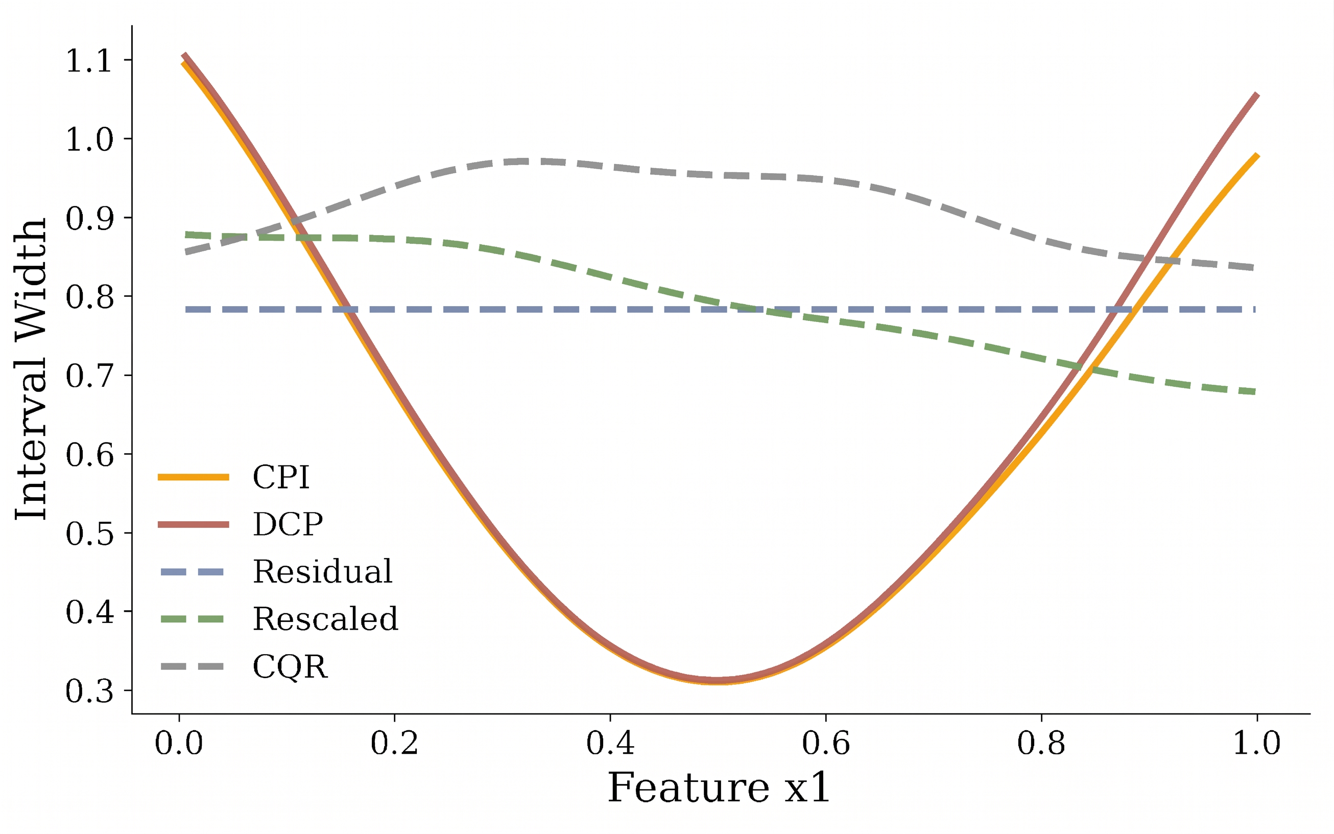
Conditional interval width. Next, we examine efficiency, measured by the width of the prediction intervals. Figure 3(b) illustrates how interval width varies with , using the same smoothing procedure as above. While the Residual, Rescaled, and CQR methods fail to adapt to the noise structure shown in Figure 3(c) and Figure 3(d), producing either constant or counter-intuitive width patterns, both CDF-based methods (CPI and DCP) exhibit U-shaped curves that closely track local variability. While CPI and DCP perform similarly over the central range of , CPI becomes more efficient near the boundaries, especially as , producing intervals approximately 5.8% shorter in the bin. This suggests that in regimes with complex noise—characterized by heavy tails or skewness—CPI achieves the target coverage with tighter intervals than DCP. As we demonstrate in the next simulation, this efficiency gap becomes even more critical under distribution shift.



5.2 Comparison between CPI and DCP under Distribution Shift
Previous simulations have assumed that calibration and test data originate from the same distribution as the training data. In practice, however, this assumption is often violated, for instance, by evolving noise structures over time. A robust conformal procedure must therefore retain valid coverage while maintaining stable efficiency. In this section, we probe this robustness through a controlled distribution-shift experiment, demonstrating how our adaptive calibration mechanism allows CPI to achieve significantly tighter, more stable intervals than DCP when the estimated CDF is systematically shifted.
Setup.
We reuse the data-generating process in Section 5.1 and introduce a location shift on the response,
| (5.1) |
applied only to the calibration and test samples; the CDF estimator (NN-CDE model) is trained on the unshifted distribution () and then held fixed. This design isolates the effect of the shift on the conformal calibration step, so that any difference between CPI and DCP can be attributed to their calibration mechanisms rather than to the underlying conditional density estimator.
| Coverage | Interval length | |||||
|---|---|---|---|---|---|---|
| bin | CPI | DCP | CPI | DCP | Red. | |
| 0.00 | 0.837 | 0.845 | 1.033 (0.259) | 1.043 (0.260) | 1.0% | |
| 0.906 | 0.909 | 0.464 (0.173) | 0.468 (0.176) | 0.9% | ||
| 0.973 | 0.976 | 0.282 (0.048) | 0.283 (0.049) | 0.6% | ||
| 0.906 | 0.908 | 0.442 (0.105) | 0.449 (0.108) | 1.5% | ||
| 0.894 | 0.902 | 0.894 (0.270) | 0.949 (0.369) | 5.8% | ||
| Marginal | 0.906 | 0.910 | 0.601 (0.334) | 0.616 (0.363) | 2.5% | |
| 0.05 | 0.866 | 0.880 | 1.116 (0.263) | 1.157 (0.256) | 3.6% | |
| 0.914 | 0.916 | 0.497 (0.181) | 0.533 (0.181) | 6.6% | ||
| 0.970 | 0.959 | 0.297 (0.047) | 0.328 (0.047) | 9.4% | ||
| 0.902 | 0.904 | 0.425 (0.108) | 0.454 (0.132) | 6.3% | ||
| 0.871 | 0.858 | 0.802 (0.216) | 1.315 (1.059) | 39.0% | ||
| Marginal | 0.906 | 0.904 | 0.603 (0.329) | 0.733 (0.630) | 17.7% | |
| 0.10 | 0.870 | 0.908 | 1.190 (0.303) | 1.505 (0.692) | 20.9% | |
| 0.914 | 0.908 | 0.513 (0.200) | 0.617 (0.211) | 16.8% | ||
| 0.948 | 0.914 | 0.298 (0.051) | 0.382 (0.053) | 22.0% | ||
| 0.916 | 0.903 | 0.457 (0.134) | 1.935 (6.398) | 76.4% | ||
| 0.903 | 0.877 | 0.919 (0.264) | 25.526 (24.892) | 96.4% | ||
| Marginal | 0.912 | 0.902 | 0.649 (0.373) | 5.965 (15.040) | 89.1% | |
Results.
Table 3 reports coverage and interval length across different shift levels (). Across all regimes, both methods successfully maintain near-nominal marginal coverage, illustrating the effectiveness of the conformal framework in providing finite-sample valid coverage through model-free calibration, even when the underlying density estimator is degraded by distribution shift. However, a significant performance gap emerges regarding efficiency. Under a mild shift (), CPI achieves a 17.7% reduction in marginal mean width, with a 39.0% reduction in the boundary bin . This efficiency gap widens dramatically under a larger shift (). In this regime, DCP becomes highly unstable; its marginal mean width reaches 5.965—nearly ten times the 0.649 value achieved by CPI. This performance degradation is even more pronounced in the bin , where DCP produces a mean width of 25.526 with a massive standard deviation of 24.892, indicating extreme sensitivity to the shift. In contrast, CPI remains robust, maintaining a mean width of only 0.919 with a standard deviation of 0.264.
6 Real Data
In this section, we evaluate the methods on six real datasets: Airfoil [3], Computer [6], Abalone [16], Concrete [29], AutoMPG [19], and Crime [20]. Each dataset is split into three disjoint subsets: for training, for calibration, and for testing, and all results are averaged over different random partitions. We compare CPI against the same four approaches as in the simulations, namely DCP, CQR, Residual, and Rescaled. All methods are calibrated at the nominal level .
Marginal coverage and interval width.
Tables 4 and 5 report the marginal coverage and average interval width on the six datasets. All methods achieve coverage close to the nominal 90% level on every dataset, confirming the validity of the conformal calibration. Under this comparable coverage, CPI consistently produces the shortest prediction intervals among all methods.
| Dataset | Residual | Rescaled | CQR | CPI | DCP |
|---|---|---|---|---|---|
| Airfoil | 0.899 | 0.913 | 0.910 | 0.902 | 0.907 |
| Computer | 0.905 | 0.903 | 0.897 | 0.897 | 0.901 |
| Abalone | 0.895 | 0.896 | 0.898 | 0.892 | 0.893 |
| Concrete | 0.884 | 0.912 | 0.897 | 0.900 | 0.910 |
| AutoMPG | 0.915 | 0.888 | 0.894 | 0.904 | 0.926 |
| Crime | 0.904 | 0.901 | 0.907 | 0.908 | 0.912 |
| Dataset | Residual | Rescaled | CQR | CPI | DCP |
|---|---|---|---|---|---|
| Airfoil | 15.34 | 12.71 | 12.42 | 11.03 | 12.31 |
| Computer | 21.75 | 25.63 | 10.62 | 8.68 | 8.71 |
| Abalone | 8.61 | 8.29 | 8.52 | 7.96 | 8.12 |
| Concrete | 34.50 | 34.92 | 31.35 | 20.82 | 22.57 |
| AutoMPG | 19.77 | 22.37 | 20.21 | 18.38 | 20.60 |
| Crime | 0.72 | 0.94 | 0.81 | 0.70 | 1.61 |
Conditional coverage.
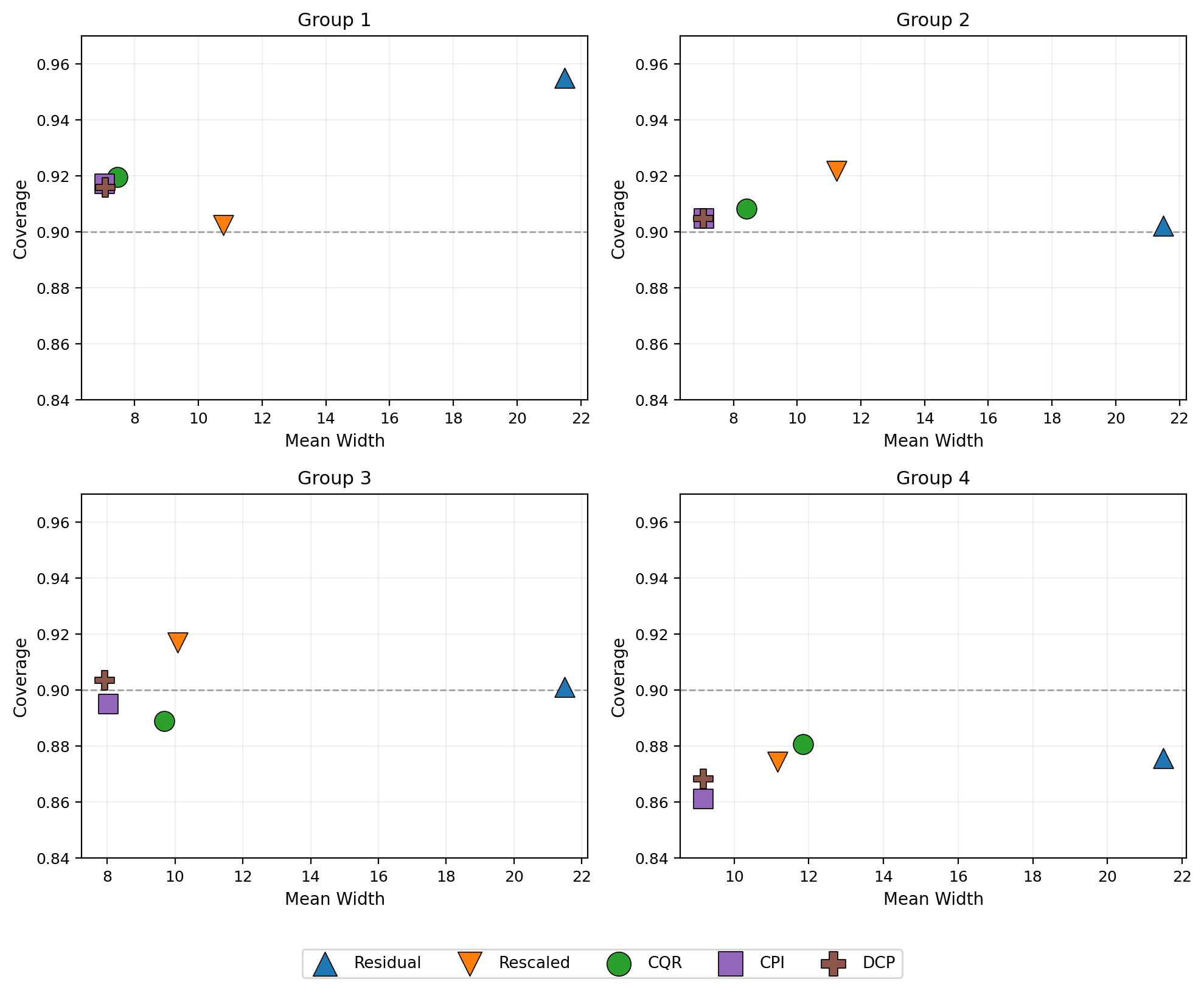
To assess conditional coverage, we project the test features onto the first principal component (PC1), computed from the standardized training data, and partition the test set into four groups according to the quartiles of the projected values. Within each group, we compute the group-specific coverage and mean interval width for each method. CPI consistently achieves the most stable coverage close to the nominal level, while yielding the shortest intervals within different subgroups across various datasets. The other four approaches either suffer from significant undercoverage in certain groups or exhibit excessively large interval widths. Figure 4 shows the results on the Abalone dataset. Across the four PC1 groups, CPI and DCP achieve coverage close to the nominal 90% level. In contrast, Rescaled slightly undercovers in Group 2, while Residual and CQR fall below the target level in Group 3. Moreover, CPI consistently achieves the shortest intervals across all four groups. These results demonstrate that CPI not only yields shorter intervals marginally but also maintains well-calibrated conditional coverage across different regions of the feature space. Analogous plots for the remaining five datasets are provided in Appendix B, where the same pattern holds consistently.

7 Discussion
In this work, we introduced a new framework for constructing prediction intervals based on conditional CDF estimation combined with a finite-sample calibration step. Our method follows the spirit of conformal prediction in using held-out data to guarantee marginal coverage, while departing from standard approaches by calibrating percentile endpoints directly rather than relying on a single conformity score. By leveraging the estimated CDF, our approach improves conditional adaptivity relative to non-CDF-based methods. At the same time, it advances existing CDF-based conformal inference by making the calibration step robust to asymmetric errors in the estimated CDF—errors that naturally arise from finite-sample bias, model misspecification, or distribution shift.
The method is simple to implement and can be paired with any conditional CDF estimator. Empirically, CPI yields more stable conditional coverage across the feature space and produces consistently shorter prediction intervals. These gains arise from better alignment with the underlying conditional distribution, rather than a trade-off between coverage and interval length.
Overall, our results suggest that directly calibrating percentile endpoints provides a flexible and effective alternative to score-based conformal methods, particularly in settings with heteroscedasticity, asymmetry, or distributional complexity.
References
- [1] (2025) PCS-uq: uncertainty quantification via the predictability-computability-stability framework. arXiv preprint arXiv:2505.08784. Cited by: §1.1.
- [2] (2024) Theoretical foundations of conformal prediction. arXiv preprint arXiv:2411.11824. Cited by: §4.
- [3] (1989) Airfoil self-noise and prediction. NASA Reference Publication Technical Report 1218, National Aeronautics and Space Administration. Cited by: §6.
- [4] (2014) Efficiency of conformalized ridge regression. In Conference on Learning Theory, pp. 605–622. Cited by: §1.1.
- [5] (2021) Distributional conformal prediction. Proceedings of the National Academy of Sciences 118 (48), pp. e2107794118. Cited by: §1, §3, §4.
- [6] (1987) Attributes of the performance of central processing units: a relative performance prediction model. Communications of the ACM 30 (4), pp. 308–317. External Links: Document Cited by: §6.
- [7] (2021) The limits of distribution-free conditional predictive inference. Information and Inference: A Journal of the IMA 10 (2), pp. 455–482. Cited by: §1, §4.
- [8] (2025) Conformal prediction with conditional guarantees. Journal of the Royal Statistical Society Series B: Statistical Methodology, pp. qkaf008. Cited by: §1.1.
- [9] (2023) Localized conformal prediction: a generalized inference framework for conformal prediction. Biometrika 110 (1), pp. 33–50. Cited by: §1.1.
- [10] (2023) Conformal prediction with local weights: randomization enables local guarantees. arXiv preprint arXiv:2310.07850. Cited by: §1.1.
- [11] (2023) Conditional distribution function estimation using neural networks for censored and uncensored data. Journal of Machine Learning Research 24 (223), pp. 1–26. Cited by: §1, §2, §5.1.
- [12] (2015) Adam: a method for stochastic optimization. In International Conference on Learning Representations, Cited by: Appendix A.
- [13] (2001) Quantile regression. Journal of Economic Perspectives 15 (4), pp. 143–156. Cited by: §1.
- [14] (2018) Distribution-free predictive inference for regression. Journal of the American Statistical Association 113 (523), pp. 1094–1111. Cited by: §1.1, §1, §1.
- [15] (2024) Conformal prediction after efficiency-oriented model selection. arXiv preprint arXiv:2408.07066. Cited by: §1.1.
- [16] (1994) The population biology of abalone (Haliotis species) in Tasmania. I. Blacklip abalone (H. rubra) from the north coast and islands of Bass Strait. Technical report Technical Report 48, Sea Fisheries Division, Department of Primary Industry and Fisheries, Tasmania. Cited by: §6.
- [17] (2025) Rectifying conformity scores for better conditional coverage. In International Conference on Machine Learning, Cited by: §1.1.
- [18] (2025) Probabilistic conformal prediction with approximate conditional validity. In International Conference on Learning Representations, Cited by: §1.1.
- [19] (1993) Combining instance-based and model-based learning. In Proceedings of the 10th International Conference on Machine Learning, pp. 236–243. Cited by: §6.
- [20] (2002) A data-driven software tool for enabling cooperative information sharing among police departments. European Journal of Operational Research 141 (3), pp. 660–678. External Links: Document Cited by: §6.
- [21] (2019) Conformalized quantile regression. Advances in Neural Information Processing Systems 32. Cited by: §1.1, §1.
- [22] (2003) Semiparametric regression. Cambridge Series in Statistical and Probabilistic Mathematics, Cambridge University Press. Cited by: §1.
- [23] (2021) Conformal prediction using conditional histograms. Advances in Neural Information Processing Systems 34, pp. 6304–6315. Cited by: §1.
- [24] (2022) Learning optimal conformal classifiers. In International Conference on Learning Representations, Cited by: §1.1.
- [25] (2019) Conformal prediction under covariate shift. Advances in Neural Information Processing Systems 32. Cited by: §1.1.
- [26] (2005) Algorithmic learning in a random world. Springer. Cited by: §1, §2.1.
- [27] (2024) Boosted conformal prediction intervals. Advances in Neural Information Processing Systems 37, pp. 71868–71899. Cited by: §1.1.
- [28] (2025) Selection and aggregation of conformal prediction sets. Journal of the American Statistical Association 120 (549), pp. 435–447. Cited by: §1.1.
- [29] (1998) Modeling of strength of high-performance concrete using artificial neural networks. Cement and Concrete Research 28 (12), pp. 1797–1808. External Links: Document Cited by: §6.
- [30] (2013) Stability. Bernoulli 19 (4), pp. 1484–1500. Cited by: §1.1.
Appendix
Appendix A Implementation Details
We provide the full implementation details for reproducibility.
NN-CDE (Hazard Network).
The conditional density estimator is a two-hidden-layer MLP with hidden units per layer and ReLU activations. All features are standardized to zero mean and unit variance. Training uses Adam [12] with learning rate , batch size , up to epochs with early stopping (patience ) on a validation split.
Optimal computation.
The shortest-width starting quantile is found by grid search over equally spaced values in . Quantile inversion uses linear interpolation on the cumulative hazard grid.
Baseline methods (simulation).
All baseline neural networks are trained with Adam (learning rate , batch size , up to epochs, early stopping with patience , validation split).
-
•
Residual: a two-hidden-layer MLP (SimpleNN) with hidden units per layer and ReLU activations, trained with MSE loss.
-
•
Rescaled: a two-hidden-layer shared backbone (MeanVarianceNN, hidden units) with separate linear heads for the mean and log-variance , trained with Gaussian negative log-likelihood loss. The conformal score is the standardized residual .
-
•
CQR: a two-hidden-layer MLP (QuantileNN) with hidden units, outputting two quantiles simultaneously, trained with pinball loss at levels and .
Real data experiments.
Each dataset is split (train/calibration/test), and all results are averaged random partitions. Our implementation follows the simulation setup with one exception: Rescaled and CQR employ a two-hidden-layer MLP with hidden units. Training is conducted using Adam with a learning rate of and a batch size of , for up to epochs with an early stopping patience of . The NN-CDE architecture and all calibration procedures remain identical.
Appendix B Conditional Coverage on Real Datasets
This appendix provides the per-group coverage vs. mean interval width plots for the five real datasets not shown in the main text. For each dataset, test points are projected onto the first principal component (PC1) of the standardized training features and partitioned into four groups by PC1 quartiles. Each scatter plot shows the group-specific coverage (vertical axis) and mean interval width (horizontal axis) for the five conformal methods, averaged over random partitions. The dashed line indicates the nominal coverage level.
Across all datasets, CPI consistently achieves coverage close to the nominal level. The sole exception is the Computer dataset, where all approaches exhibit undercoverage in Group 4. Notably, CPI maintains the narrowest prediction intervals in each PC1 group, confirming that its marginal interval width advantage extends to the conditional setting.