Statistical Inference of Day-to-Day Traffic Dynamics
Abstract
Day-to-day traffic dynamics are widely used to model flow evolution due to travelers’ learning and adjustment behavior, yet empirical analysis of these models often relies on descriptive calibration with limited inferential content. This paper develops a statistical inference framework for day-to-day route choice dynamics based on a stochastic individual-level adjustment model. The framework enables uncertainty quantification and formal inference for behavioral parameters from trajectory data. We establish identifiability and consistency under mild conditions, and extend the framework to accommodate demand variation, user heterogeneity through a hierarchical structure, and anonymized observability caused by privacy constraints on trajectory data. Simulation studies demonstrate good finite-sample performance, calibrated uncertainty, and robustness to model misspecification. Empirical analyses of controlled laboratory experiments and real-world trajectory data from Ann Arbor, Michigan, show that the framework can generate novel behavioral insights across settings: it reveals the inadequacy of a purely inter-day learning model once en-route information is introduced, recovers systematic behavioral differences across participant types, and uncovers meaningful day-to-day learning together with substantial demand variation in real-world commuting behavior.
keywords:
Day-to-day dynamics, Bayesian inference, Vehicle trajectory data, Identifiability, User heterogeneitynewfloatplacement\undefine@keynewfloatname\undefine@keynewfloatfileext\undefine@keynewfloatwithin
1 Introduction
Day-to-day traffic dynamics are widely used to model flow evolution due to travelers’ learning and adjustment behavior. From a system-level perspective, day-to-day traffic dynamics provide valuable insights into how traffic patterns evolve over time (watling2013modelling). Through theoretical analysis of its convergence and stability, researchers aim to establish a behavioral justification for the concept of user equilibrium (wardrop1952road), a cornerstone for transportation network analysis and planning methodology. At the individual level, day-to-day route choices reflect travelers’ learning and adaptation behaviors. One example is the Smith dynamics (smith1984stability), which captures user inertia through gradual route swapping, as travelers shift from higher-cost routes to lower-cost routes. More broadly, the literature has incorporated a range of behavioral mechanisms about how travelers learn, adjust, and respond to congestion over time (horowitz1984stability, guo2011bounded, he2012modeling).
As illustrated in Figure 1, existing day-to-day models can be broadly divided into two types: deterministic and stochastic. Both are primarily concerned with the forward problem, namely, specifying how behavioral parameters govern the day-to-day evolution of traffic states. Using path flow as the system state for illustration, deterministic models treat the state on a given day as a deterministic function of the previous state, thereby representing population-average dynamics (watling1999stability). Some of these models capture emergent behavior from micro-behavioral rules (horowitz1984stability), whereas others directly model aggregate adjustment dynamics (smith1984stability). Stochastic models, by contrast, explicitly characterize the random realization of travelers’ daily choices, so that the state on each day is drawn from a probability distribution (davis1993large, cantarella1995dynamic, hazelton2002day, hazelton2004computation, QI2024100123).

Despite substantial theoretical progress in forward modeling, the inverse problem, recovering behavioral parameters from empirical data, remains a significant and underexplored challenge. A large body of empirical work has relied on deterministic forward models, reducing estimation to the minimization of a prediction error, which essentially functions as model calibration (mahmassani1990dynamic, mahmassani2000transferring, srinivasan2003analyzing, ye2018exploration, qi2023investigating, guo2011bounded, he2012modeling, cheng2019surrogate). Although this approach is useful and easy to implement, it has important limitations. Because deterministic models do not assign probabilities to the data, they typically yield only point estimates and do not provide a likelihood-based framework for inference. As a result, calibration-based methods are difficult to quantify estimation uncertainty, which limits their usefulness for downstream behavioral analyses and decision-making. For example, when comparing behaviors across cities, point estimates may differ, but without quantified uncertainty, it is difficult to determine whether those differences are statistically meaningful.
Stochastic day-to-day models offer a natural remedy by providing the probabilistic foundation needed for statistical inference on behavioral parameters. However, only a small number of studies have moved in this direction. Seminal work by parry2013bayesian, hazelton2016statistical jointly inferred path flows and behavioral parameters from observed link flows. However, their system state, path flows, have long been considered unobservable and non-identifiable from standard loop detector data (yang2018stochastic). In such settings, multiple latent path-flow processes, potentially associated with different behavioral parameters, can be observationally equivalent at the link-flow level. This makes the identification of the underlying behavioral parameters difficult to establish. Admittedly, other day-to-day models are formulated using observed link flows as system states (he2010link). However, this comes at the cost of behavioral interpretability, since individual route choice behavior is no longer modeled explicitly.
Recent advances in connected vehicle and GPS technologies have fundamentally altered this situation. High-resolution trajectory data are now increasingly available, and unlike loop detector counts, they offer direct visibility into individual path choices and even how travelers adjust routes from day to day. This new data regime resolves the long-standing observability bottleneck and provides sufficient structure for the identification of behavioral parameters. At the same time, enhanced observability opens the door to richer behavioral modeling. Travelers naturally exhibit heterogeneous responses to experienced costs: long-term residents with stable travel habits may have low sensitivity to cost differences, whereas newcomers still learning the network may be far more responsive. Trajectory data can allow us to track individuals over time and model this heterogeneity explicitly, moving well beyond the average flow patterns that have constrained much of the prior literature.
To address these opportunities, this paper proposes a statistical inference framework for individual day-to-day route choice behavior. We first introduce an individual-level route adjustment model grounded in established day-to-day dynamics. Building on this model, we develop a Bayesian estimation framework that provides full uncertainty quantification rather than point estimates alone. We theoretically establish model identifiability and prove consistency of the estimation procedure under mild regularity conditions, thereby providing a rigorous foundation for inference. We further extend the framework to accommodate anonymized observability caused by common data privacy constraints, and to incorporate traveler heterogeneity through a hierarchical structure. For validation, the proposed method is thoroughly examined in a simulated small-scale network to evaluate estimation performance and verify theoretical properties. It is then applied to lab experiment datasets and high-resolution trajectory data from Ann Arbor, Michigan, to generate novel behavioral insights.
Our paper develops a complete inferential framework for the inverse problem of stochastic day-to-day models. Specifically, we make the following contributions:
-
•
Rigorous inferential foundation: We establish identifiability and consistency for a Bayesian framework applied to stochastic day-to-day models, properties that prior calibration-based approaches cannot provide. This clarifies both what is being estimated and whether reliable estimation is theoretically feasible.
-
•
Uncertainty quantification. By adopting a Bayesian approach, we move beyond point estimation and characterize the full posterior distribution over behavioral parameters, enabling principled statistical inference.
-
•
Traveler heterogeneity. We explicitly model and estimate heterogeneous behavioral parameters across individuals through a hierarchical structure, recovering the population distribution of adjustment behavior rather than a single aggregate value. To the best of our knowledge, this is the first study to do so.
-
•
Empirical insights. We apply the framework to both controlled lab experiments and real-world trajectory data from Ann Arbor, Michigan, generating novel behavioral insights.
The remainder of this paper is structured as follows. Section 2 presents the model, our estimation approach, and theoretical results. Section 3 extends the model to anonymized observability and incorporates user heterogeneity. Section 4 provides simulation studies on a synthetic network, and Section 5 applies the proposed method to analyze behaviors in lab environments and real-world routing scenarios. Finally, Section 6 concludes the paper.
2 Model and Estimation
To facilitate the presentation of our approach, we begin with a simplified setting in which all commuters are assumed to be homogeneous. This specification is commonly referred to as the pooled model. Section 3 later extends the framework to a hierarchical model that captures user heterogeneity. As we focus on the commuting problem, we use the terms travelers and commuters interchangeably.
2.1 Individual Day-to-Day Choice Model
Let denote the study group of commuters, a sample from the total demand, where is the total number of observed commuters. To better present our approach, we first consider a single origin-destination (OD) pair. Let denote the set of available paths and the time horizon. The travel cost of path on day is denoted by and is treated as exogenously given. The daily cost vector is written as , and we assume that the cost is always bounded by a finite constant . In practice, demand may also vary over time. To accommodate this feature, we treat non-travel as a virtual alternative, denoted as path 0.
We use a random variable to represent the path chosen by commuter on day , including the virtual non-travel path, with support . To simplify notations, we denote the full choice sequence of commuter over the time horizon by , which is a random vector on . The collection of choice sequences of all commuters is denoted by , defined on .
On each day, each commuter chooses not to travel with a constant probability , which is driven by exogenous needs such as remote work, rather than cost-based elasticity. The resulting choice probabilities are
| (1) |
For physical paths, initially, each commuter is assumed to have limited information about path costs and other travelers’ behavior. We therefore set the initial perceived cost for each physical path to for all commuters and paths . Alternatively, the initial valuation could be set to free-flow travel time without affecting the structure of the model. After observing realized travel costs, commuters update their perceived costs using an exponential smoothing rule:
| (2) |
where is the learning rate that captures the sensitivity of each commuter to newly observed travel costs.
Given the perceived costs, each commuter chooses a path according to a multinomial logit model, conditioned on traveling on that day. Specifically, for ,
| (3) |
where is the scale parameter, and -algebra refers to the flow of information over time up to day , which essentially consists of the history of the travel costs.
For notational convenience, we denote the probabilities in Equations (1) and (3) by . In the pooled model, all commuters are assumed to share common behavioral parameters and therefore identical choice probabilities, denoted by without the commuter index.
Following the daily choice process, the probability of observing a full choice sequence for a single commuter, , is given by
| (4) |
We further assume that commuters make their daily route choices independently, conditional on their perceived costs. Although commuters influence one another through congestion effects embedded in the realized travel costs, conditional independence holds at the decision stage given the perceived valuations. Under this assumption, the probability of observing a full set of choices across all commuters, , is
| (5) |
This framework extends naturally to multiple commodities under the assumption that commuters associated with different OD pairs make independent decisions based on their own perceived costs. With a slight abuse of notations, let denote the number of commuters within OD pair , and let denote the choice sequence of commuter within OD pair . Then, the joint probability becomes
| (6) | ||||
Adding OD pairs increases computation complexity in the log-likelihood only linearly. From a computational perspective, multiple OD pairs are equivalent to having more commuters within a single OD pair. As a result, the presence of multiple commodities does not fundamentally alter the structure of the model. For notational simplicity, we therefore focus on the single-OD setting in the remainder of this section.
The proposed model describes route adjustment through two components, an exponential smoothing rule for updating perceived costs and a logit model for translating perceived costs into choice probabilities. This structure is grounded in the behavioral foundation of Horowitz dynamics (horowitz1984stability):
| (7) |
| (8) |
Here, and refer to the perceived and true cost on path of OD pair on day , respectively. represents the path flow and refers to the demand.
Despite sharing similar behavioral components, Horowitz dynamics, as well as most existing day-to-day models, are formulated at the aggregate path-flow level. In addition to allowing for varying demand, a key distinction of our proposed model is complete observability at the individual level: the daily path choices of each studied commuter are directly observed, which is available in high-resolution trajectory data and is also naturally satisfied in laboratory route-choice experiments. By retaining individual choice trajectories rather than only aggregate counts, the proposed formulation provides the foundation needed to infer behavioral parameters and, in Section 3, to accommodate user heterogeneity.
Nonetheless, Proposition 1 shows that this richer individual-level model remains consistent with the classical aggregate perspective as the number of commuters increases. Similar observations have also been made by davis1993large and watling1999stability. Proofs throughout the paper are provided in Appendix B.
Proposition 1.
The structure of the model above is summarized in Figure 2.

2.2 Estimation algorithm
We now turn to estimation of the parameters after observing a realized set of choice trajectories, .
At first glance, the individual-level formulation appears to induce a state space that grows exponentially with the number of commuters. However, this combinatorial explosion does not enter likelihood evaluation. For estimation, we only need to evaluate the probability of the realized individual trajectories observed in the data, rather than enumerate all possible population states. Because the joint likelihood factorizes across commuters and days under conditional independence, computation scales with the observed data rather than with the size of the full state space.
Specifically, to ensure numerical stability and computational efficiency, we work with the log-probabilities:
| (9) |
| (10) |
for all . The complete-data log-likelihood for the realization is therefore
| (11) | ||||
where are indicator variables. The resulting likelihood function is differentiable with respect to .
We adopt a Bayesian inference approach, as it is more robust in settings with limited or noisy data. We assume independent prior distributions for the parameters, so that . The choice of prior families is motivated by the parameter domains. Since , we assign logit-normal priors, which place mass on the unit interval while remaining flexible in shape. Since , we assign a log-normal prior, which places mass on the positive real lin. Thus, the posterior distribution satisfies
| (12) |
In practice, we compute the log-posterior:
| (13) | ||||
The Bayes estimator is taken as the posterior mean. For example,
| (14) |
and similarly for and .
Beyond point estimation, statistical inference requires uncertainty quantification. We report marginal Highest Density Intervals (HDIs) as credible intervals (CIs) for each parameter, which is the narrowest range that can cover certain proportions of the posterior. For a confidence level (e.g., 95%), the HDI for is defined as
| (15) |
where refers to the marginal posterior, and the threshold satisfies:
| (16) |
Similar for the other two parameters.
Because the likelihood and posterior do not admit closed-form expressions and must be evaluated recursively through the latent valuation updates, direct posterior evaluation is infeasible. We therefore rely on sampling-based methods that approximate the posterior via empirical distributions. Given posterior draws , then
| (17) |
The -credible interval is
| (18) |
where
| (19) |
The same procedure applies to the other two parameters.
Because and interact multiplicatively in the likelihood, the posterior over can exhibit strong correlations: a higher and a lower perceived cost difference can produce similar choice probabilities, creating elongated, curved posterior ridges that standard random-walk Markov chain Monte Carlo (MCMC) traverses inefficiently. We therefore adopt the No-U-Turn Sampler (NUTS) (hoffman2014no), an adaptive variant of Hamiltonian Monte Carlo (HMC) (girolami2011riemann). HMC uses gradient information to propose distant moves along the posterior geometry, greatly reducing the autocorrelation of samples compared to random-walk methods, especially in correlated posteriors. Readers are referred to hoffman2014no for details of the algorithm’s implementation.
2.3 Theoretical results
The estimation algorithm above is well-defined only if the parameters it targets are identifiable and the estimator is consistent. We now establish both properties formally.
2.3.1 Identifiability
Identifiability characterizes what parameters can be uniquely learned from the data, independently of the estimation method or sample size.
Definition 1 (Identifiability).
For a given cost sequence , the model is identifiable if
| (20) | ||||
for all indicates .
If identifiability fails, multiple distinct parameter values generate the same likelihood functions. Hence, no amount of data or estimation methods can tell them apart. In such cases, estimation becomes fundamentally ill-posed. We establish identifiability under a rather weak condition on the cost sequence.
Assumption 1 (Dynamic richness).
There exists at least one pair of distinct routes, , such that their sequence of cost difference, , do not always equal , where and .
Theorem 1.
The model is identifiable if and only if the cost sequence satisfies Assumption 1.
A useful intuition for the necessity of Assumption 1 is that identification of the learning rate requires temporal variation in perceived value differences. If Assumption 1 fails, the induced perceived value differences remain constant over time, so there are no effective learning dynamics. In that case, different values of generate the same choice probabilities.
2.3.2 Consistency
Identifiability is a property of the model and data-generating process: it ensures that the parameter-to-likelihood mapping is injective. Consistency is a property of the estimator: it guarantees convergence to the true parameter values as more data becomes available.
Definition 2 (Consistency).
Let denote the model parameters with true value . Define . The estimator is consistent if, for all ,
| (21) |
Identifiability alone does not guarantee consistency. For example, if the cost sequence satisfies Assumption 1 only over a finite initial period and becomes constant thereafter, learning effectively stops, which prevents the estimator from converging to the true values. This motivates a stronger requirement: the cost sequence must remain persistently informative throughout the horizon.
Assumption 2 (Persistent excitations).
Let denote the true parameters. The cost sequence satisfies that for any , there exists such that for all with :
| (22) |
where refers to the choice probabilities under parameter , and represents KL divergence.
Intuitively, this assumption ensures that any parameter sufficiently far from the truth keeps generating choice distributions that are persistently distinguishable from those under , that is, the KL divergence between them does not vanish. This is the condition that forces the posterior to eventually reject wrong parameter values.
Under this condition and standard regularity assumptions, consistency can be established. For tractability, we focus on the case that is known, for example when demand variation has been pre-calibrated. The main technical challenge in allowing to be estimated is that the non-travel indicator complicates the uniform convergence argument. We leave this extension for future work.
Theorem 2.
Suppose:
-
•
is known;
-
•
The parameter space ;
-
•
True parameter is in the interior of ;
-
•
The prior is continuous and satisfies .
Then, under Assumption 2, the estimator is consistent.
2.4 Endogenizing initial values
The baseline model above assumes exogenously specified initial valuations, such as zeros or the free-flow travel times. While reasonable for newcomers with no prior experience, this assumption may be unrealistic for long-term residents who have already accumulated information.
A natural remedy is to treat the initial valuations as additional model parameters to be estimated. However, this creates a non-identifiability: because multinomial logit choice probabilities depend only on relative costs, any global shift in the initial valuations leaves the likelihood unchanged.
Proposition 2.
For any feasbile , the parameter sets and , where for any constant and , are observationally equivalent and thus not identifiable.
To resolve this issue, we parameterize initial conditions using relative differences , . This pins down the location of the initial valuations up to the irrelevant global shift, introducing additional parameters. Identifying these additional degrees of freedom requires a somewhat stronger condition on the cost sequence.
Assumption 3 (Stronger dynamic richness).
The vectors in contain at least three linearly independent elements.
This assumption requires that the cost sequence exhibits sufficient linear variation over time, essentially, that the data are rich enough to separately pin down the initial offsets from the learning rate . It is still mild in practice: any cost sequence with moderate temporal variation will satisfy it. The following theorem recovers identifiability for the model with endogenized initial values.
Theorem 3.
Under Assumption 3, the model with parameters is identifiable.
3 Model Extensions
So far, we have established a statistical inference framework for the pooled model under full observability of homogeneous travelers. In this section, we extend the framework to incorporate two more realistic features: user heterogeneity and anonymized observability.
3.1 User Heterogeneity
The pooled model characterizes all commuters using a single set of parameters, assuming homogeneous behavior. While this yields tractable estimation, it cannot recover the distribution of behavioral parameters across individuals, even though this distribution is itself a primary object of interest. We therefore introduce a hierarchical Bayesian model that treats individual parameters as random draws from a population distribution, and estimates that distribution directly from the data.
Before proceeding, it is worth clarifying why the pooled posterior distribution cannot simply be reinterpreted as the population distribution of behavioral parameters. Although this may seem natural, it is generally misleading. To illustrate, consider a coin-flipping experiment in which denotes the probability of heads. Suppose the data are generated either (i) by a homogeneous population with , or (ii) by a heterogeneous population in which each individual has with equal probability. Both scenarios produce identical observations. As the sample size grows, the posterior distribution for concentrates at in both cases, even though the underlying population distributions of are fundamentally different. The same issue arises here: a pooled estimate of tells us the average learning rate across commuters, but reveals nothing about whether some commuters are fast learners and others are slow. Recovering that heterogeneity requires a model that explicitly represents it.
3.1.1 Model
As demonstrated in Figure 3, we assume each traveler draws an individual parameter vector from a population distribution governed by hyperparameters . Given , traveler ’s day-to-day choices follow the same individual model as in Section 2.1. We denote the hyperpriors by .

The choice of population distributions is flexible. A convenient specification that respects parameter constraints while allowing asymmetric shapes is:
-
•
Logit-normal for and
(23) (24) -
•
Log-normal for
(25)
Under this specification, the hyperparameters are . We place normal hyperpriors on the location parameters and half-normal hyperpriors on the scale parameters . The half-normal is supported on , which enforces non-negativity of the scale while providing mild regularization near zero and preventing the posterior from collapsing to .
With heterogeneous parameters, the day- choice probabilities become
| (26) |
| (27) |
for all . We retain the notation for these probabilities with minor abuse of notation.
Formal identification of the hyperparameters requires a mixture identifiability argument that combines Theorem 1 with properties of the logit-normal family; we leave a rigorous treatment for future work. In practice, is estimable when both and are sufficiently large, as individual parameters become well-identified with large based on previous theorems, and their population distribution becomes recoverable with large , which will be further illustrated in simulation studies in Section 4.
3.1.2 Estimation
The complete-data log-likelihood under the hierarchical model is
| (28) | ||||
The joint posterior over individual parameters and hyperparameters is
| (29) | ||||
In practice, we sample jointly from this full posterior using NUTS. Marginal estimates for the hyperparameters and for each individual parameter vector are then read off directly from the posterior draws. The Bayes estimator and individual estimates are taken as posterior means, and credible intervals are computed via HDIs as in Section 2.2.
However, directly sampling over can exhibit numerical pathologies, known as Neal’s funnel geometry (neal2003slice). The problem arises because the geometry of the posterior changes drastically with : when is large, the individual parameters can vary widely; when is small, all must lie very close to , creating a narrow ridge of high posterior mass that is difficult for HMC-based samplers to explore accurately. The step size that works well in the wide regime is far too large for the narrow regime, leading to either poor exploration or rejected proposals.
To improve posterior geometry, we employ a non-centered parameterization for all hierarchical parameters. For example,
| (30) |
and similar for the and . This formulation preserves the same generative process as the centered model but decouples the latent individual offsets from the scale parameters . The posterior over is now approximately standard normal regardless of , yielding a well-conditioned geometry that NUTS can explore efficiently across the full range of hyperparameter values.
3.2 Anonymized Observations
The preceding sections assumed complete individual-level observability, motivated by the emergence of high-resolution trajectory data. However, privacy regulations may require that user identifiers be reshuffled or anonymized on a daily basis, so that daily route counts are available but individual trajectories cannot be linked across days. Note that this observability issue considered here should not be confused with another separate problem of recovering path flows from link-level observations.
3.2.1 Observation model
We introduce the following observation model shown in Figure 4. As discussed earlier, we still present the model for a single OD pair, which can be easily extended to multiple commodities.
On each day , we observe an -dimensional vector , where each element denotes the number of commuters choosing that route, including the virtual “not traveling” option:
| (31) |
We write and denote the full observation sequence as .

3.2.2 Pooled model
Under the pooled model, shown in Figure 4(a), all travelers share the same behavioral parameters and initial values. Hence for all and all .
Because all commuters draw independently from the same categorical distribution , the observed count vector follows a multinomial distribution:
| (32) | ||||
Therefore, for a realized observation sequence, the likelihood function is:
| (33) |
Taking logs yields
| (34) | ||||
The log-posterior is then obtained by adding the log-priors as in the fully observable case.
Interestingly, anonymized observability does not weaken identifiability in the pooled model.
Proposition 3.
Similar for the model with endogenized initial values:
Proposition 4.
The key reason is permutation invariance: since all commuters share the same choice distribution under the pooled model, the likelihood is unchanged if we permute the labels of any two commuters. This means that only aggregate counts matter for inference and individual identities carry no additional information. The following theorem formalizes this equivalence and reveals what identifiability in the pooled model truly requires.
Theorem 4.
For any realized choice sequence and its corresponding aggregate observations , the two posteriors are equal:
| (35) |
for all
This theorem indicates that individual-level data and aggregate count data are informationally equivalent for the purpose of recovering . Therefore, identifiability in day-to-day models hinges not on the granularity of individual tracking, but on the observability of the path flow over time.
3.2.3 Hierarchical model
The pooled case is convenient because all commuters share the same choice distribution, yielding multinomial observations. In the hierarchical model with anonymized observability (Figure 4(b)), this convenience no longer holds: different travelers may have different parameters and initial values, leading to different choice distributions . The aggregate count vector now follows a Poisson-multinomial distribution (PMD) (lin2022poisson):
| (36) |
The first two moments are
| (37) |
| (38) |
where denotes the diagonal matrix with entries .
However, the PMD does not admit a simple closed-form likelihood, and exact computation is too expensive to embed inside an MCMC sampling loop. We therefore adopt an approximation. During sampling, whenever the likelihood is needed, we approximate by a multinomial random vector
| (39) |
where .
Proposition 5.
For all ,
| (40) |
The proposition indicates that this approximation matches the mean exactly but overestimates variance. To see the magnitude, consdier the binary case :
| (41) |
which vanishes as heterogeneity in individual choice probabilities decreases. The direction of the approximation error matters for inference: because the multinomial approximation overestimates variance, the resulting likelihood is more diffuse than the true PMD likelihood, which tends to produce wider and more conservative credible intervals.
4 Simulation Studies
In this section, we evaluate the proposed estimation approach in a controlled synthetic environment. The goals are to (i) demonstrate the computation, and (ii) empirically validate the theoretical properties established earlier.
4.1 Experiment Setup
We generate background traffic using the standard Nguyen–Dupuis (ND) network setting (nguyen1984efficient), with four OD pairs . Background traffic evolves according to Horowitz dynamics with zero initial valuations. To avoid convergence to a fixed equilibrium and to mimic real-world variability, we add Gaussian noise to the path valuations each day. We simulate the background dynamics for 20 days as a warm start, and we assume observations begin on day 21.
As shown in Figure 5, we then introduce a study group of commuters traveling from Node 5 to Node 11, with three feasible paths: , and . Because this group is small relative to background traffic, we assume it does not affect the path costs generated by the background dynamics (i.e., costs are treated as exogenous for the study group).

We evaluate performance using three metrics:
-
•
Mean bias: measures the accuracy of the point estimation;
-
•
Empirical coverage of 95% CI: evaluates the calibration of uncertainty. An estimator may be nearly unbiased yet still produce misleading uncertainty estimates, which undermines statistical inference and downstream decision-making.
-
•
Width of the 95% CI: among estimators with similar coverage, a narrower interval indicates greater information extraction and higher precision from the same data.
4.2 Pooled Models
4.2.1 Estimation results
We first conduct a parameter recovery study under the pooled model. Specifically, we draw “true” parameter triples independently from the estimation prior: , .
For each parameter triple, we generate choice sequences under the fixed travel cost sequence while varying (i) the horizon length and (ii) the number of travelers . For each simulated dataset, we compute posterior point estimates and corresponding 95% intervals.
Figure 6 shows an example of the estimated joint posterior and marginals from a single run. The posterior samples appear approximately Gaussian, suggesting well-behaved inference in this setting. In this example, exhibits a larger deviation than and , which is unsurprising because has broader support and enters multiplicatively with valuations, making it harder to pin down.

Because any single run is noisy, we summarize performance across all 1,000 trials. We report sampling diagnostics and model-fit checks in Appendix 6.1. Figure 7 reports average bias under different settings. In the upper row, we fix and increase from 1 to 20; in the bottom row, we fix and increase from 10 to 50. Overall, bias decreases as information increases, consistent with Theorem 2. Some non-monotonicity remains due to finite-sample randomness.
Interestingly, increasing is more effective than increasing . Intuitively, longer horizons provide more observations but also propagate latent-valuation uncertainty through the recursive updates, whereas increasing provides more independent sequences at each . Finally, tends to be easier to estimate because it affects travel or not directly and is less entangled with the other two parameters.

Figure 8 presents empirical coverage of 95% CI across simulation settings. Coverage remains close to the nominal level across horizon lengths and numbers of travelers, indicating good finite-sample calibration and reliable uncertainty quantification in these settings.
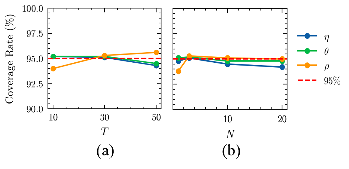
Figure 9 reports the average width of the 95% CI. Interval widths decrease monotonically as either or increases, reflecting increasing posterior concentration and again aligning with the consistency result in Theorem 2. This also indicates that as information accumulates, the estimator becomes more confident.

4.2.2 Robustness to misspecification
We also examine the robustness of the pooled estimator to model misspecification. Specifically, we consider (i) prior misspecification, where data are generated from alternative parameter distributions, and (ii) behavioral misspecification, where data are generated from heterogeneous agents or from a Smith-type swapping model (smith1984stability) rather than Horowitz dynamics.
Across these settings, misspecification increases bias and reduces coverage relative to the correctly specified case, but overall performance degradation remains moderate. Importantly, aggregate flow predictions remain accurate when heterogeneity is ignored, while misspecifying the behavioral mechanism itself leads to larger extrapolation errors. Nevertheless, richer information (e.g., more commuters, longer horizon) improves the performance and yields acceptable extrapolation accuracy. Detailed results and analysis for these experiments are provided in Appendix 6.2.
4.3 Hierarchical Models
This section moves beyond the pooled model to directly recover population heterogeneity.
4.3.1 Estimation results
We conduct a hyperparameter recovery study. We draw true hyperparameter vectors from the distributions in Table 1. Condition on hyperparameters , each traveler draws their individual parameters via , and then generates choices under the fixed cost sequence.
Figures 10 and 11 report average bias for the six hyperparameters under varying and . In general, increasing systematically improves estimation, which is expected because a larger population provides more information about between-user dispersion. In contrast, increasing has a much smaller effect. Intuitively, longer horizons help identify each individual’s behavior more precisely, but provide limited additional information about user heterogeneity once individual parameters are already reasonably identified.


We further examine uncertainty quantification for hierarchical parameters. Empirical coverage of 95% credible intervals remains close to the nominal level across most settings, and interval widths decrease monotonically with increasing , reinforcing that population size is the dominant source of information for learning heterogeneity. In contrast, increasing yields diminishing returns once individual-level behavior is sufficiently identified. Detailed coverage and interval-width results are reported in Appendix 6.3.
4.3.2 Model misspecification
We next ask whether the hierarchical estimator can recover population-level behavior when the assumed population distributions are misspecified. This matters in practice because the true distributions are rarely known.
We generate individual parameters using: . Because “true” pooled parameters no longer exist under misspecification, we evaluate extrapolation accuracy instead of parameter recovery. Specifically, we estimate the model using the first days and predict choice probabilities for the next days. To remove finite-agent randomness, we compare predicted choice probabilities against the true probabilities rather than against realized discrete choices.
Figure 12 shows that predicting aggregate choice probabilities is relatively easy: even with and , the model captures the main fluctuation patterns with minor level shifts. However, recovering the population distribution is substantially harder: with small , the estimated distribution can deviate notably from the truth (Figure 13(a)). As increases, the estimator observes a wider range of behaviors, and population distribution estimates improve. Increasing further improves both distribution recovery and predictive accuracy. Remarkably, for and , extrapolated choice probabilities nearly overlap with the truth.


4.3.3 Anonymized observability
Because we have shown that anonymized observability does not affect the pooled model in Section 3.2.2, we focus here on the hierarchical model.
Table 2 reports the true values of hyperparameters and their estimates under complete versus anonymized observability. While posterior means for location parameters, such as , are similar across settings, anonymized observability substantially underestimates dispersion (e.g., . Figure 14 illustrates this effect using individual estimates: anonymized observability yields much less variation across individuals.
The underlying reason is the weak identifiability of heterogeneity under aggregate count data. Individual heterogeneity is inherently permutation-sensitive, whereas aggregate counts are permutation-invariant. As a result, groups with different within-population dispersions can generate similar aggregate behavior when their mean choice tendencies are similar. This suggests that anonymized observable data may be sufficient for predicting aggregate flows, but it provides limited behavioral insight into population-level parameter distributions.
| True | - | 0 | 1.0 | -2.0 | 1.0 | |
| Complete observability | -1.5 | 0.48 | 0.33 | 0.84 | -1.7 | 0.74 |
| Anonymized observability | -1.5 | 0.22 | 0.31 | 0.31 | -1.6 | 0.24 |

5 Empirical Analysis
In this section, we examine the empirical performance of the proposed framework in both experimental and real-world settings.
5.1 Controlled Laboratory Experiments
We first study two controlled laboratory experiments, which allow us to assess model adequacy under different information regimes and to compare latent behavioral parameters across participant types.
5.1.1 A study on information provision
The first route-choice experiment is based on wijayaratna2017experimental, illustrated in Figure 15(a). The network follows a Braess-type structure, except that one link is stochastic: link C–B takes cost 20 with probability 20% and cost 1 with probability 80%. Participants complete two conditions. The first is a no-information condition, in which route choices are committed at departure, and commuters have to rely on their own experiences. The second setting incorporates information provision, in which the realization of link C–B is revealed at node C and travelers may revise their decisions.

We begin with the no-information condition and fit the proposed model with initial perceived values all set to 0. Unlike in the simulation study, there is no ground-truth choice probability available in the laboratory data, so model assessment must rely on the realized sample path. For this reason, we focus on in-sample posterior predictive performance rather than extrapolation as in Section 4. Specifically, for each posterior draw, we generate 500 replicated path counts over the experimental horizon and summarize the predictive distribution using the Monte Carlo mean together with 50% and 95% predictive intervals.
Figure 32 in Appendix 6.4 shows that, under the no-information condition, the model captures most of the observed day-to-day variation in path counts. Although finite-sample fluctuations remain substantial, the realized frequencies are generally well covered by the predictive bands. This suggests that, when travelers commit to a route, the proposed day-to-day learning model provides a reasonable explanation of the observed variation.
We then endogenize the initial perceived values, and the result is shown in Figure 16. This modification improves the posterior predictive fit, suggesting an interesting insight: participants may enter the experiment with nontrivial prior perceptions rather than a completely undifferentiated initial view of the network. Moreover, the path containing the stochastic link (ACBD) tends to receive a higher estimated initial perceived cost by 1.42. While the model does not separately parameterize risk attitudes, this pattern is consistent with the possibility that participants initially discount alternatives involving uncertain costs.

We next fit the same class of model to the en-route information condition. As shown in Figure 17, the fit deteriorates substantially: several features of the observed path-count variation are not captured by the posterior predictive distribution, especially for path ACBD when the stochastic link is realized at a high cost. By contrast, the predictive performance for path ABD remains reasonable, since this path is not meaningfully affected by the en-route information. The natural interpretation is that information provision alters the underlying behavioral mechanism in a way that is not well captured by a purely day-to-day updating framework. Adequately representing behavior under information provision may therefore require a richer model that incorporates both day-to-day and intra-day learning.

5.1.2 A study on behaviors across participant types
We next turn to the experiment of wang2025comparing, illustrated in Figure 15(b). In this environment, participants, including human participants, GPT-4, GPT-3.5, and reinforcement-learning (RL) agents, traverse a route consisting of four successive segments. On each segment, they choose between two alternatives, and after completing each segment they receive congestion information from the preceding link. This creates a richer adaptive setting with repeated feedback and within-trip adjustment opportunities. In the main analysis, we represent these repeated decisions at the finer segment level, which better matches the feedback structure of the experiment. A comparison with a coarser path-level representation is reported in Appendix 6.4. We fit the model separately to datasets generated by different participant types. Since initial values are less sensitive for longer horizons, we fix them in these experiments.
To compare behavioral differences across participant types, we adopt the Region of Practical Equivalence (ROPE), a well-established Bayesian hypothesis testing approach designed to assess whether an effect is large enough to be practically meaningful (kruschke2010bayesian, kruschke2014doing). Because the parameter is scale-dependent and thus less directly comparable across settings, we focus our inference on whether the learning rates are meaningfully different. A key challenge is that does not have a linear effect on behavioral outcomes. For example, increasing from 0.05 to 0.1 doubles the updating weight on new information, whereas increasing from 0.55 to 0.6 is comparatively minor. Following kruschke2018rejecting, we instead test on the logit scale. For example, when comparing human and GPT-4, we define , and set ROPE to . Equivalently,
| (42) |
Intuitively, reflects the relative weight placed on today’s experience versus prior beliefs under exponential smoothing. Hence, this ROPE corresponds to treating differences of roughly in the new-versus-old weighting as practically negligible.
Figure 18 summarizes the corresponding posterior contrasts. The results reveal systematic differences across groups. In panel (a), which compares humans with GPT-4, over 97% of the posterior lies below . This provides strong, one-sided evidence that the learning rate of GPT-4 has a meaningfully higher learning rate than humans, indicating greater sensitivity to the previous day’s experienced costs. In panel (b), the posterior contrast with GPT-3.5 is shifted in the opposite direction, suggesting that humans exhibit a higher learning rate than GPT-3.5. By contrast, the posterior in panel (c), which compares humans with reinforcement-learning agents, is fairly centered around 0. However, only 2% of the posterior mass lies within the ROPE, so the two groups cannot be regarded as practically equivalent. At the same time, the posterior does not concentrate strongly on either side, so the difference between humans and reinforcement-learning agents is not clearly distinguishable under the current data.

These differences are also reflected in the posterior predictive performance shown in Figure 33 in Appendix 6.4, where GPT-4 exhibits substantially greater volatility than the other three participant types, and are broadly consistent with the findings in wang2025comparing. The proposed framework provides a principled way to assess whether such observed differences correspond to meaningful differences in underlying behavioral parameters.
5.2 Real-world Trajectory Data
We now turn to trajectory data from Ann Arbor, Michigan, to examine commuter behavior in a real-world setting.
5.2.1 Dataset and preprocessing
The Ann Arbor network has 632 road junctions and 1,583 road segments. The road features and network skeleton were sourced from a benchmark trip-based travel demand forecast model developed for the SEMCOG 2050 Regional Forecast (semcog_regional_forecast). Vehicle trajectory data were collected during the evening peak (4:30–5:30 PM) from March 1 to May 31, 2022, capturing stable travel patterns within the academic semester. Following the map-matching methodology in wang2023trajectory, the sample yielded an average of 3,127 daily trips, which were utilized to calculate link features (such as link travel time). To identify main traffic patterns, we included OD pairs observed for at least 14 days.
From all valid OD pairs in the dataset, we select three pairs that feature meaningfully distinct routes. We exclude OD pairs whose routes differ only marginally, such as two nearly symmetric ways to traverse a square, where observed choices are largely driven by noise or improvisation rather than systematic learning. Figure 19 illustrates one of the selected OD pairs; the remaining two are presented in Appendix 6.5.
In the OD pair shown, commuters travel from the university hospital area to the interchange of highways M-14 and I-94 when exiting Ann Arbor. Two clearly differentiated routes are available: a highway route (red) and a local-road route through downtown (blue). Summary statistics for this OD pair are reported in Table 3. The highway route has a lower average travel time, with slightly higher variability, and is chosen more frequently. Over the 66-day observation period, at most 10 commuters per day are observed for this OD pair. We therefore fix the total daily demand at 10 for this OD pair, as the demand parameter would not be identifiable without this normalization.

| Local | Highway | |||
| Cost (min) | Counts | Cost (min) | Counts | |
| Mean | 11.90 | 0.94 | 11.02 | 2.06 |
| Std | 0.98 | 1.10 | 1.00 | 1.63 |
5.2.2 Pooled model esitmation
We first estimate the pooled model to recover population-average behavioral parameters. The results are reported in Table 4, where denotes the initial value difference for OD pair .
One notable feature of real-world data is substantial day-to-day demand variation. In this dataset, each commuter has more than a 60% probability of not traveling on a given weekday. Such flexibility, likely influenced by remote work, is rarely present in lab experiments but is central in modern commuting behavior. The estimated negative value of indicates that commuters initially perceive the highway route as more attractive than the local route for the OD pair in Figure 19, which is broadly consistent with the observed cost statistics.
| Estimates | 0.024 | 0.39 | 0.61 | -2.4 | 0.066 | 2.1 |
Given this result, it is natural to ask whether this day-to-day learning is practically meaningful. We therefore test whether the estimated is meaningfully different from 0. Because is not well-defined, we assess practical equivalence of directly using the ROPE . We choose , which corresponds approximately to an half-life of exponential smoothing over 66 days, the length of the observation period. This is a fairly large threshold for practical equivalence: it treats as negligible even learning rates for which the initial belief is reduced by half over the course of the study. Figure 20 shows that more than 83% of the posterior mass lies above this ROPE. Thus, the data provide substantial evidence that real-world commuters engage in meaningful day-to-day learning, indicating that day-to-day modeling has behavioral relevance in practice.

5.2.3 Hierarchical model and behavior dispersion
Although we showed in Section 4.3.3 that anonymized observability weakens identification of heterogeneity, we nevertheless estimate the hierarchical model to gain qualitative insight into the distribution of behaviors across the population. Figure 21 reports the implied population distributions of individual parameters based on the estimated hyperparameters. As discussed earlier, dispersion may be underestimated due to anonymized observability. Key findings include:
-
•
Learning rate : highly concentrated between 0 and 0.1. Nearly all commuters place less than 10% weight on new daily information relative to accumulated beliefs. It indicates that some proportion of commuters are doing meaningful day-to-day updating, but strong inertia persists and makes updates very gradual.
-
•
Costs sensitivity : moderately dispersed, with most mass between 0.1 and 0.7. This indicates meaningful variation in responsiveness to perceived cost differences.
-
•
Demand parameter : exhibits the widest dispersion. Only a small fraction commute nearly every weekday, while more than half of commuters stay home at least half of the time. This highlights substantial flexibility and the importance of modeling demand variability explicitly when analyzing real-world commuter behavior.

6 Conclusion
This paper develops a Bayesian inference framework for day-to-day route choice behavior that moves beyond descriptive calibration to support uncertainty quantification, hypothesis testing, and rigorous behavioral analysis. The central theoretical contributions are formal identifiability and consistency results that clarify when and how behavioral parameters can be recovered from observations, properties that prior calibration-based approaches neither establish nor require. The framework accommodates demand variation, user heterogeneity through a hierarchical extension, and anonymized observability motivated by privacy constraints on trajectory data.
Simulation studies confirm that the estimator achieves good finite-sample performance: bias shrinks systematically as the observation horizon grows, and credible intervals are well-calibrated across a range of parameter configurations. Importantly, robustness analyses show that aggregate flow predictions and population distribution estimates remain stable under moderate model misspecification. Hence, the framework degrades gracefully when behavioral assumptions are imperfectly met, which is a necessary condition for practical applicability.
The empirical analysis shows that the proposed framework can generate novel behavioral insights from both experimental and real-world data. In controlled laboratory experiments, it reveals that the day-to-day learning model explains much of the observed variation under no-information conditions. Once en-route information is introduced, however, the same model becomes inadequate, indicating that richer information changes the decision process in ways not well captured by a purely inter-day updating mechanism. A second laboratory application recovers systematic behavioral differences across participant types: humans appear less reactive than GPT-4, more reactive than GPT-3.5, and broadly comparable to reinforcement-learning agents. In the real-world Ann Arbor data, the results provide substantial evidence of meaningful day-to-day learning, while also revealing considerable demand variations.
Several directions remain for future research. First, the inference structure developed here, exponential smoothing of perceived costs combined with a logit choice rule, is not specific to route choice. With appropriate reformulation, the same framework can be applied to other behavioral dynamics, such as departure time adjustment or mode choice adaptation with appropriate reformulation. Second, while the hierarchical model provides qualitative insight into heterogeneity, stronger identification of population distributions under anonymized observability remains an open theoretical problem. It may require richer data sources, alternative model designs, or a full mixture identifiability argument that we have left for future work. Finally, extending the consistency analysis to settings with an unknown demand parameter would close the remaining gap in the theoretical foundation.
Acknowledgement
The work described in this paper was partly supported by research grants from National Science Foundation, United States (CMMI-2233057 and 2240981). The authors thank Xinhe Wang, Naichen Shi, and Ran Sun for valuable feedback.
References
Appendix A. Proof of Main Results
Proof for Proposition 1.
As the valuations follow the exact same updating process as in Horowitz dynamics, we only need to consider the choice probability, which results in path flow following the observation , detailed in Section 3.2.2.
As discussed in that section, , its expectation follows:
| (43) |
which matches the path flow in Horowitz dynamics.
The path flow observation satisfies
| (44) |
and is i.i.d categorical with . Thus, by the strong law of large numbers,
| (45) |
which proves the proposition.
Proof for Theorem 1.
First, the following lemma indicates that we only need to prove identifiability for a system with only one commuter.
Lemma 1.
If for any , the model is identifiable if
| (46) |
indicates .
Proof for Lemmea 1.
Suppose we have the identifiability for a model with only one commuter. When the following equation holds:
| (47) |
it must also hold for the case where all commuters replicate the choice of commuter . Therefore,
| (48) |
In the pooled model, all commuters share the same choice distribution, hence this equation implies that Equation (46) also holds. Therefore, .
Let us now consider the system with , and we prove sufficiency first. We drop the superscripts for clarity and write as .
For a chosen pair of routes , let . The valuation difference follows the exponential smoothing as well:
| (49) |
Suppose the model is not identifiable. That is, two parameter sets are observationally equivalent:
| (50) |
It must hold for a specific choice sequence , where the commuter always chooses not to travel. In this case, the equality can be rewritten as:
| (51) |
which indicates .
In addition, for actual path choices , let and be the values generated by under the same cost sequence . This requires:
| (52) |
which indicates
| (53) |
If there exists a pair such that , we have . Based on the assumption, there must be . Besides, it further indicates that for all . Denote it as . Now, we prove that for all , and by induction.
First, for any pair , we have
| (54) |
It further indicates , and thus . Therefore, we have .
Now suppose holds for and for all pairs . We further have
| (55) |
which again indicates . Therefore, it also holds for . By induction, we prove the property.
Consequently, we have
| (56) |
which indicates that for all and . Therefore, is a constant for all pairs, which contradicts the Assumption 1.
As a result, we must have for all . Now, we prove for all and by induction. We already showed that it holds for .
Now suppose it holds for with . We have for all . Equation (53) indicates that
| (57) |
If there exists such that , then . Denote the value as . We further have:
| (58) |
| (59) |
Equation (53) indicates that
| (60) |
It further implies , and thus , which contradicts the non-identifiability assumption.
Therefore, it must be for all , which leads to . As a result, the conclusion also holds for . By induction, we prove that for all . As , we have for all , which contradicts Assumption 1.
Consequently, our assumption does not hold, and the model is identifiable, which proves the sufficiency.
Now, let us focus on necessity. The following lemma indicates that the perceived value differences remain constant over time.
Lemma 2.
If Assumption 1 does not hold, for all .
Proof for Lemma 2. Let us prove it by induction.
For any pair , we have
| (61) |
which means that the claim holds for .
Suppose it also holds for with , then . Therefore,
| (62) |
As a result, the claim also holds for . By induction, we prove the claim.
Therefore, if Assumption 1 fails, the learning rate never enters the logit choice probability on any day:
| (63) | ||||
| (64) | ||||
| (65) | ||||
| (66) |
for all .
As a result, different generate the same likelihood function, thus it is not identifiable, which proves the necessity.
Proof for Theorem 2.
We only need to prove a simplified case with . The general case only differs by a constant and known multiplier of , which has no influence on consistency.
Denote the choice probability as
| (67) |
Define a random function for the random variable , which takes value of for each possible choice . Define a general log-likelihood function for the random sequence
| (68) |
which is also a random function.
Define:
| (69) |
which can be rewritten as
| (70) |
The centered value can be rewritten as:
| (71) | ||||
| (72) |
where denotes the choice distribution vector.
The posterior can be written as
| (73) | ||||
| (74) |
and thus the goal is to prove the numerator decays faster than the denominator as .
We first prove a lemma regarding .
Lemma 3.
For any ,
| (75) |
Proof for Lemma 3 First, it is easy to show that is uniformly bounded; thus, is also uniformly bounded according to the regularity assumptions, which further indicates that is also uniformly bounded. Denote the bound as , i.e., , and thus for all and .
Because is fixed, essentially becomes a random variable, which is independently but not identically distributed for each . We further have
| (76) |
Its expectation satisfies:
| (77) |
Therefore,
| (78) |
By the Strong Law of Large Numbers, we have
| (79) |
as .
To simplify notations, let us denote , for any . This random function can be proved to be uniformly Lipschitz continuous.
Lemma 4.
There exists a constant , such that for any , for all and realization of .
Proof for Lemma 4 It is easy to see that the value function is uniformly bounded, i.e., for all . We further have
| (80) |
Let us prove by induction on . This holds for automatically. Suppose it also holds for :
| (81) |
Therefore, it also holds for , which proves the claim.
Now, let us prove that the has a bounded gradient. The log-likelihood can be written as:
| (82) |
Therefore,
| (83) | ||||
| (84) |
which indicates that
| (85) |
Meanwhile,
| (86) | ||||
| (87) |
which leads to
| (88) |
As a result,
| (89) |
which further indicates that for all .
As is convex, based on the Mean Value Theorem, for any fixed realization of ,
| (90) |
Because takes vales in a finite set , and the gradient is uniformly bounded for any , we have
| (91) |
Meanwhile,
| (92) | ||||
| (93) |
which indicates .
Finally,
| (94) |
The Lipschitz continuity further ensures that the convergence is not only pointwise as in Lemma 3 but also uniform.
Lemma 5.
| (95) |
Proof for Lemma 5 Based on the Lipschitz continuity in Lemma 4, for any , there exists such that for all with , .
Since is compact, it is separable, which means that it can be covered with a finite number of open balls of radius . Denote the centers as . Thus, for any , it is within distance from some center .
For any , from Lemma 3, as . Therefore, there exists such that for all , almost surely. Let , thus for all , almost surely for all .
Consequently, for any , find closest center where , then for all :
| (96) |
Note that is independent of , therefore
| (97) |
which proves the uniform convergence.
Now we are ready to prove the consistency. For any , the numerator in Equation (74) satisfies:
| (98) | ||||
| (99) | ||||
| (100) |
Hence, for sufficiently large
| (101) |
Consequently, the numerator satisfies
| (102) |
Define a small ball , whose size decreases with . Thus, it is easy to see that for sufficiently large , for all due to the continuity of the prior.
For any :
| (105) |
which indicates
| (106) |
As a result, the denominator satisfies:
| (107) | ||||
| (108) | ||||
| (109) |
Finally,
| (110) |
Proof for Proposition 2.
As discussed in Lemma 1, we only need to consider a model with . Again, we omit the superscript and denote the two value functions as and .
Since two parameter sets share the same , and the MNL model is shift-invaraint, as long as
| (111) |
and will always generate the same choice probability, hence are not identifiable. We now prove this by induction on .
First, it automatically holds for . Suppose it also holds for . Then, the exponential smoothing indicates
| (112) |
and
| (113) |
for all . Therefore, the equation also holds for . By induction, we prove the proposition.
Proof for Theorem 3.
Similar to our proof for Theorem 1, we only need to consider a simplified case where , and is identifiable.
Suppose the model is not identifiable. That is, two parameter sets have the same choice probabilities, where and represent the vector form of the initial value parameters. If , the two initial values are essentially the same despite constant shifts. In that case, there will not be two distinct parameters that are not identifiable according to Theorem 1. Therefore, there must be . Equation (53) indicates that , or simply in a vector form, which further ensures that .
and cannot both be zero; thus without losing generality, we assume . For a non-zero vector, Assumption 3 ensures that it must be linearly independent of at least two vectors from . Let us denote the first two linearly independent vectors as and , with .
By repeatedly substituting , we get the unrolled form:
| (114) |
and similar for .
A similar equation also holds for . The following two equations cannot hold simultaneously
| (117) |
otherwise , which further indicates and contradicts the assumption.
Without losing generality, assume . Due to the linear independence, cannot have component from , thus there must be
| (118) |
Substituting and into Equation (53), we have:
| (119) |
As for some , we have , which further leads to . These results contradict our assumption.
Therefore, the starting assumption does not hold, and the model is identifiable.
Proof for Proposition 3.
We omit the proof as it can be proved following a similar way as in Proposition 4.
Proof for Proposition 4.
In the pooled model, all commuters share the choice probability. Denote the choice probability generated by parameter as .
We first present the following lemma. As the observation likelihood is given by a multinomial distribution, this lemma can be proved by Corollary 6.16 in lehmann1998theory.
Lemma 6.
If for all observation and , there must be for all and .
Now, suppose the model is not identifiable, meaning that there exist two different parameter sets , such that for all observation and . Lemma 6 ensures that these parameter sets also ensure for all and , which contradicts the identifiability in Theorem 3. Therefore, the assumption does not hold, and the model is identifiable.
Proof for Theorem 4.
The posterior of the anonymized observation model satisfies
| (120) |
where the likelihood function equals:
| (121) |
Thus, the log-posterior satisfies:
| (122) |
Meanwhile, for the fully observable model, we denote the choice probability as for all . We have
| (123) |
and further
| (124) |
where the final equality holds because in , there are number of , for .
Therefore, the log-posterior satisfies:
| (125) |
which only has a constant shift relative to the anonymized case. As the posteriors need to sum up to one, they must be identical.
Proof for Proposition 5.
For expectations:
| (126) |
For variance:
| (127) |
We have
| (128) | ||||
| (129) |
where the diagonal terms cancel out because diag is a linear operator.
Let . Then, . Expand:
| (130) |
As each matrix is positive semi-definite (PSD), the sum of PSD matrices is also PSD, which proves that .
Appendix B. Additional Results
6.1 Bayesian Diagnostics
Here we present the sampling diagnostics for the pooled model with .
The first metric is the split , which assesses convergence by comparing within-chain and between-chain variance. Figure 22 shows that all the empirical distribution concentrates at 1.00, indicating satisfactory convergence.

Figure 23 presents the histogram of the effective sample size (ESS), which measures the sampling efficiency at the center of the posterior. For all three parameters, ESS is mostly above 2500, indicating efficient exploration of the posterior.

Figure 24 presents the empirical distribution of the normalized rank of the true parameter value in the samples, which detects the bias and poor mixing. Rank histograms are approximately uniform for all parameters, suggesting no detectable bias or pathological sampling behavior.

6.2 Robustness to Misspecification
6.2.1 Shift in parameter generation
In practice, the modeler rarely knows the true parameter-generating distribution. A common source of modeling bias is prior misspecification. To test robustness, we generate data under two alternative distributions that differ from the estimation priors:
-
•
Same distribution families but different parameters:
-
•
Different distribution families:
Figure 25 visualizes these distributions. As expected, the shapes differ substantially from the estimation prior.

Figure 26 summarizes estimation performance under these scenarios. Overall, misspecification degrades performance, increasing bias and reducing coverage, but the deterioration remains within an acceptable range. In contrast, the effect on interval width is comparatively small: interval width mainly reflects how much information can be extracted from a given dataset under the chosen model, and moderate prior misspecification has limited influence on that extraction efficiency. Among the parameters, is the least affected by the distribution shift, consistent with its relatively clean identifiability through the travel/no-travel mechanism.

6.2.2 Model misspecification
Beyond prior misspecification, we evaluate robustness under two more challenging model misspecifications. For clarity, we assume no demand variation (i.e., ) and only estimate the other two more challenging parameters:
-
•
Heterogeneous behaviors: data are generated by travelers with heterogeneous parameters, but we still fit the pooled model.
-
•
Different behavioral model: Wtravelers follow a Smith-type swapping rule (smith1984stability). Starting from a uniform random choice over paths, on day , a traveler who previously chose path switches to another path with probability:
(131) and thus
(132) Intuitively, commuters on a high-cost option will switch to lower-cost options at a rate that is proportional to the cost difference. Here we set to ensure probabilities remain valid.
Because “true” pooled parameters no longer exist under misspecification, we evaluate extrapolation accuracy instead of parameter recovery. Specifically, we estimate the model using the first days and predict choice probabilities for the next days. To remove finite-agent randomness, we compare predicted choice probabilities against the true probabilities rather than against realized discrete choices.
Figure 27 shows posterior samples under different settings. In the heterogeneous-behavior case (panel (a)), the pooled estimator lies near the center of the individual-level “true” parameter cloud, consistent with estimating an average effect. Compared with Figure 6, the posteriors under misspecification are more irregular, reflecting a mismatch between model and data. Nonetheless, increasing information, such as increasing and , yields more concentrated and better-behaved posteriors (panel (c)).

Figure 28 reports extrapolation performance. Prediction is highly accurate for heterogeneous behaviors (panel (a)), indicating that even when individual-level behavioral interpretation is limited, aggregate outcomes can still be predicted well from a pooled approximation. In contrast, extrapolation is substantially worse under behavioral-model misspecification (panel (b)), suggesting that misspecifying the adjustment mechanism is more damaging than ignoring heterogeneity. Nevertheless, increasing and improves performance and yields acceptable extrapolation accuracy.

6.3 Hierarchical Model Estimations
Figure 29 reports empirical coverage for 95% intervals and shows rates close to nominal. Some degradation appears for large or , likely due to increased computational difficulty (e.g., divergences or poorer mixing), which can reduce effective sample size and slightly distort interval calibration.

Figures 30 and 31 report average widths of the 95% CIs. Width decreases monotonically with , reinforcing that population size is the main driver for learning heterogeneity. When increases from 30 to 50, widths for most hyperparameters stop decreasing, suggesting that roughly 30 days already contain sufficient temporal information in this synthetic setting and additional days yield diminishing returns.


6.4 Controlled Lab Experiments
Figure 32 presents the predictive performance of the model with fixed initial values on the no-information data.

Figure 33 presents the posterior predictive performance for the four participant types. In general, the predictive bands cover the realized frequencies well. In contrast, Figure 34 shows the results for the 40-day coarse path-level data, where the predictive mean is almost stationary and fails to capture path-count variations.


6.5 Trajectory Data
Figure 35 gives the other two OD pairs in the experiment. Both involve two routes: one goes through highways and the other utilizes local roads.
