- CG
- Computer Graphics
- CNN
- Convolutional Neural Network
- CPU
- Central Processing Unit
- CV
- Computer Vision
- DL
- Deep Learning
- DNN
- Deep Neural Network
- EPE
- Endpoint Error
- FPS
- Frames per second
- GPU
- Graphics Processing Unit
- GAN
- Generative Adversarial Network
- K
- Kilo, thousand
- M
- Million
- MB
- Megabyte
- ReLU
- Rectified Linear Unit
- SSIM
- Structural Similarity Index Measure
- PSNR
- Peak Signal-to-Noise Ratio
- FID
- Fréchet Inception Distance
- LPIPS
- Learned Perceptual Image Patch Similarity
- MPJPE
- mean per-joint point error
- MPJPE-PA
- Mean Per Joint Position Error after Procrustes Analysis
- PVET
- Per-Vertex-Error in T-Pose
- KID
- Kernel Inception Distance
- IS
- Inception Score
- LPIPS
- Learned Perceptual Image Patch Similarity
- LDM
- Latent Diffusion Model
- DM
- Diffusion Model
- SD
- Stable Diffusion
- XDoG
- eXtended difference-of-Gaussians
- NST
- Neural Style Transfer
![[Uncaptioned image]](2605.02583v1/graphics/teaser/original.jpg)
SD unedited output
![[Uncaptioned image]](2605.02583v1/graphics/teaser/blackpointlower_masked.jpg)
-black point
![[Uncaptioned image]](2605.02583v1/graphics/teaser/depthcontrast_teasre.png)
+highlights
![[Uncaptioned image]](2605.02583v1/graphics/teaser/lwedit.jpg)
+stroke width
![[Uncaptioned image]](2605.02583v1/graphics/teaser/linewidth_color_teaser.png)
+colorfulness
![[Uncaptioned image]](2605.02583v1/graphics/teaser/baroque_back_1.jpg)
+realism
![[Uncaptioned image]](2605.02583v1/x1.jpg)
![[Uncaptioned image]](2605.02583v1/x2.jpg)
Increase watercolor splattering
![[Uncaptioned image]](2605.02583v1/graphics/teaser/room_gogh.jpg)
![[Uncaptioned image]](2605.02583v1/graphics/teaser/room_gogh_depthpower.jpg)
Increase local contrast
![[Uncaptioned image]](2605.02583v1/graphics/teaser/earring_inverted.png)
![[Uncaptioned image]](2605.02583v1/graphics/teaser/earring_linewsithd3.jpg)
Editing of a real image
Stylistic Attribute Control in Latent Diffusion Models
Abstract
Text-to-image diffusion models have revolutionized image synthesis and editing, but precise control over stylistic attributes remains a challenge, often causing unintended content modifications. We propose an approach for fine-grained parametric control of stylistic attributes in latent diffusion models by learning disentangled editing directions from synthetic datasets. We use guidance composition to close the domain gap between stylistically finetuned and foundation models, preserving the original image semantics while applying stylistic adjustments. To ensure consistent edits, we introduce a training regularization loss and enhance DDIM inversion with optimized null-conditional embeddings for real image editing. We validate our approach by learning from stylistically filtered synthetic datasets varying a range of stylistic attributes, including outlines, local contrast, watercolorization effects, and geometric patterns. Our evaluations demonstrate that compared to current text-based editing techniques, our method offers well-integrated, more precise and continuously adjustable stylistic modifications.
1 Introduction


Generative diffusion models, especially latent diffusion models (LDMs) such as Stable Diffusion (SD) [rombach2022high], have revolutionized image synthesis, producing remarkably detailed outputs from text prompts [rombach2022high, betker2023improving]. Text-to-image models learn a vast range of styles from large-scale paired data, surpassing previous methods in fidelity and diversity. Recent methods like ControlNet [zhangAddingConditionalControl2023] and T2I-Adapter [mouT2IAdapterLearningAdapters2023] improve layout control, while text-based editing [hertz2022prompt, brooksInstructPix2PixLearningFollow2023, zhang2024magicbrush] can replace objects or alter global style. However, such methods often struggle at fine-grained editing of stylistic elements like color, texture, and stroke patterns due to prompt ambiguities, unintended content modifications and inability to control edits on a continuous scale. Thus, a Photoshop-like editing workflow, allowing artist to adjust parameter sliders for specific aspects of the style in a controlled manner during image generation is currently not possible.
Earlier filter-based non-photorealistic rendering (NPR) methods[Kyprianidis:2013:SAT], allow fine grained parameter control (e.g., line width in Fig.˜11(b)), but they operate on low level features and often fail to capture scene semantics, a shortcoming that has repeatedly been mentioned as motivation for methods such as Neural Style Transfer (NST) [Gatys2016ImageST, Jing_2020_NST] and content-aware tone pipelines [gharbi2017deep]. Moreover, as filters are applied post-synthesis they cannot benefit from shared scene understanding and user intent, such as the text- or geometry-guidance during reverse diffusion. For instance, increasing edges using a NPR-based edge filter thickens all edges equally (Fig.˜11(b)), whereas our LDM-integrated approach (Fig.˜11(c)) selectively places stylistic emphasis on object contours and important features (e.g., tree stems).
Our approach introduces a method to apply parametric control over specific stylistic attributes, where attribute strength and location can be precisely controlled in SD generation. Such adjustments are difficult to define through text alone and are often entangled in style image references, making traditional style transfer methods unsuitable, yet are easily generated as small synthetic datasets of desired adjustments. For example, varying outline strength and sensitivity in an edge filter [winnemoller2012xdog], we can fine-tune an adapter for outline control in SD generation (Fig.˜11(c)). In Fig.˜10 we demonstrate control over attributes such as brush stroke width, local contrast, highlighting, blackpoint, effect-specific controls such as watercolor paint splattering, as well as real image editing.
However, directly finetuning adapters on desired stylistic attributes often results in domain shifts away from the original SD distribution and can degrade output quality and diversity. To mitigate this, we re-align the output latents to the SD domain using guidance composition and introduce a training regularization that discourages undesired semantic changes. For real-image editing, we adapt null-text inversion [mokadyNULLTextInversionEditing], optimizing null-parameter embeddings for stable reconstructions. Our experiments demonstrate that this integrated approach can precisely adjust stylistic attributes without undesired changes to the image semantics or global style. Compared to previous approaches, our edits can furthermore be adjusted on a continuous scale, allowing slider-based fine-grained style control. We plan on releasing the code and pretrained models.
2 Related Work
2.1 Traditional Image Filtering Techniques
In contrast to deep learning, traditional image-based artistic rendering (IB-AR) methods [Kyprianidis:2013:SAT] offer granular control through a series of engineered filters designed for specific artistic styles. Although highly controllable, these methods are constrained to specific, handcrafted styles like cartoon, oilpainting or watercolor effects [winnemoller2006real, semmo2016image, bousseau2006interactive] or stroke-based [liu2021paint, zou2021stylized] or learnable filter-based [lotzsch2022wise, reimann2024artistic] de- and re-composition of images. Further, their post-hoc filtering is not informed of high level semantics and user intent that the text-to-image generative methods are given, such as prompt and spatial guidance, reducing their ability for content- and style aware adjustments. We make use of IB-AR for synthetic data generation of parameter-controllable stylistic attributes, where our fine-tuned controls do not seek to exactly replicate the effects of filter application but to provide an editing direction to the LDM along the range of the filter-parameter.
2.2 Diffusion-based Control Techniques
Methods such as ControlNet [zhangAddingConditionalControl2023] and T2I-Adapter [mouT2IAdapterLearningAdapters2023], have enabled spatial control of Diffusion Models [sohl2015deep, dhariwal2021diffusion] by integrating guidance maps. Many methods explore prompt-based semantic editing of images, like the training-free prompt-to-prompt [hertz2022prompt] and null-text inversion [mokadyNULLTextInversionEditing], which manipulate the attention and guidance vectors of Latent Diffusion Models during inference, as well as the model-training based InstructPix2Pix [brooksInstructPix2PixLearningFollow2023], MagicBrush [zhang2024magicbrush] and, specifically for styles, StyleBooth [han2024stylebooth], which learn instruction-based editing. In our work, we make use of ControlNet for spatial guidance and demonstrate that out proposed approach is better suited for disentangled editing of specific stylistic elements like color, texture, and stroke patterns, and is significantly better for continuous scale editing than these instruction-based editing methods.
3 Method

Let denote an image generated by denoising a latent , which is either sampled from random noise or obtained by inversion of a real image. Our goal is to edit by precisely adjusting specific stylistic attributes globally or locally, controlled by continuous parameter strengths , resulting in an edited image . These parameter-based adjustments of global and local image properties must be learned explicitly from a dataset encoding the desired stylistic attributes with varied strengths , as textual prompts alone lack the precision required for such edits. Naively fine-tuning the diffusion model directly on such datasets however results in a domain shift characterized by reduced diversity and compromised generative quality due to the comparatively small and less content-diverse target datasets. We formalize this as a covariate shift, where the original Stable Diffusion model defines a source domain distribution conditioned on text prompts , and the dataset of stylistically edited images defines a narrower target domain distribution . To address this covariate shift, we finetune a LDM (we follow standard LDM [rombach2022high] notation, see suppl. for background) designed to steer image generation toward the target stylistic attributes, and extract the attribute representations using a guidance formulation at inference. To maintain alignment with the source domain distribution, the isolated stylistic guidance from is composed with the original diffusion model output at each denoising step of the reverse diffusion process.
In the following, we detail our guidance-based composition strategy (Sec.˜3.1), approach to maintain spatial stability (Sec.˜3.2), and network training approach (LABEL:{subsec:method:network}). Furthermore, we extend this technique to real image editing through null-embedding inversion outlined in Sec.˜3.4.
3.1 Effect Guidance
After fine-tuning on an effect-specific dataset, we isolate the learned stylistic control in from layout, semantic and other stylistic appearance features inherent in the training data. To this end, we define a editing vector towards our desired edit by encoding as the difference between noisy predictions at the desired stylistic strength and the neutral baseline ():
| (1) |
Note that we do not supply prompt embeddings () to both networks. Since guidance vectors are compositional [liu2022compositional], we can then introduce our fine-tuned guidance vector to the text-conditioned base SD () classifier-free guidance [hojonathanClassifierFreeDiffusionGuidance2022] as:
| (2) |
where are classifier free guidance scales.
3.2 Spatial Stability

While applying the above formulation to an conditioned solely on text can yield visually compelling results (Fig.˜13), the outputs often lack spatial stability. Minor variations early in the diffusion process can lead to significantly different image layouts. To address this, we fix the coarse spatial layout by conditioning both and on spatial maps, utilizing a ControlNet [zhangAddingConditionalControl2023]. We use Canny edge image conditioned ControlNets as spatial anchors due to their generality and ease of creation. Specifically, is steered using a pretrained Controlnet, receiving , while is steered using our A-finetuned Controlnet (see Fig.˜12). The predicted noise using classifier guidance is thus actually
| (3) |
where and represent the ControlNet-conditioned prompt and attribute guidance vectors. Spatial conditioning significantly enhances consistency and reduces unintended correlations between layout and stylistic effects. However, regions lacking clear spatial features (e.g., without edges) may still experience unintended semantic alterations. To mitigate such content drift, we activate stylistic guidance after timestep , restricting semantic freedom of . Formally, we set guidance activation as for , with normalized between 0 (start) and 1 (end) of denoising. We empirically set to balance effect strength and stability, further complemented by a training regularization term detailed in Eq.˜4.
3.3 Network
Architecture.
We use a ControlNet architecture and insert a layer with an extra attention transformer-block after the text-conditional cross attention into the overall downsampling blocks. The extra attention layer receives an embedding of the input parameters . During training, only the extra attention layers and the -embedder are finetuned, preserving the original weights of the LDM. Ablation studies (Sec.˜4.2) show that this variant keeps the results more stable compared to finetuning the cross attention blocks or encoding parameters into tokens.
Training Regularization.
During inference, changes introduced into the image often get more drastic with increased parameter values , which also includes unwanted semantic changes. These are encoded in the guidance term between the zero-conditional and the parameter term. To combat this, we introduce a regularization term. Intuitively, the regularization aims at penalizing the difference of images produced with and at spatial locations that do not correspond to changes in the input training images. Let be a latent sample obtained from noising the image of effect strength after one step of DDIM [song2020score]. Further, let be the latent where the effect was not applied. The regularization loss is then defined as:
| (4) |
Training Loss.
We finetune the ControlNet attention blocks using the well-known diffusion training strategy [song2020denoising, dhariwal2021diffusion, rombach2022high]. We extend the training loss of ControlNet [zhangAddingConditionalControl2023] to incorporate our conditioning on parameter , fixed guidance maps and the training regularization, which is controlled with strength . The training loss for a timestep is then defined as:
| (5) |
3.4 Real image editing
Let be a real image. To achieve image editing of , we have to invert into noise . DDIM inversion [dhariwal2021diffusion] reverses the diffusion process, transforming an encoded real image back into a noise vector through incremental steps of reversed DDIM. However, DDIM inversion alone is not sufficient to capture good editing directions for prompt-based editing [mokadyNULLTextInversionEditing], as inversed latents can diverge from their original trajectory due to the guidance scale amplifying reconstruction errors, resulting in bad editing results. To remedy this, Mokady et al. [mokadyNULLTextInversionEditing] propose to also optimize the null-text embedding during inversion. The optimized null text embedding hereby plays the role of a pivot towards a more editable direction in CfG latent space. First, the DDIM inversion is performed with CfG guidance scale and outputs a sequence of initial latent codes . These are then used as targets for the optimization of the null text embedding , minimizing the error between and , which is the latent code obtained from a step of DDIM sampling with guidance . This procedure is repeated in each timestep, initialising and with the previous step results, and yielding optimized embeddings. Please refer to Mokady et al. [mokadyNULLTextInversionEditing] for details on the algorithm.
We adapt this approach, but instead of optimizing the null-text embedding, we optimize the null-parameter () embedding used in . Further, compared to the original formulation, we invert Eq.˜3, including the applications of the two controlnets. Thus, for every timestep we optimize for N iterations
| (6) |
During image editing inference, the stored noise latent and optimized null-parameter conditional embeddings can then be injected to edit the parameters. Joined optimization of both text and null conditions leads to degraded results, as we show in an ablation experiment (Sec.˜4.2).
4 Experiments


4.1 Training Dataset
Synthetic.
We generate synthetic training datasets by creating multiple stylized renditions of content images with a stylization filter , varying the strengths of its parameters for each image. Our variations concern only specific attributes of the effect, not the overall effect intensity, i.e., at , the stylization effect (e.g., watercolorization) remains visible. We generate the following datasets, using MSCOCO train2014 [MSCOCO] as content images:
-
•
Watercolor. We use a watercolorization filter [bousseau2006interactive], adjusting seven parameters: “contourWidth" (Fig.˜14(a)) and “details" for controlling outlines and fine brushstrokes; “colorfulness" and “blackpoint" (Fig.˜14(b)) for histogram adjustments; watercolor-specific effects such as “paintSplatter” and “wobbling"; and “depthPower" (Figs.˜14(c) and 14(d)) for adaptive contrast enhancement [gharbi2017deep].
-
•
Cartoon. We employ a cartoonization filter [winnemoller2006real], which combines color quantization with thick outlines generated by eXtended difference-of-Gaussians (XDoG).
-
•
Stroke Rendering. We utilize PaintTransformer [liu2021paint] using coarse brushstrokes to create a stroke-based aesthetic (Fig.˜15).
Real Artworks.
We train on Artbench [liao2022artbench], containing real artworks for different styles, and create photographic versions of each using a Controlnet conditioned on the artwork canny edge maps. This allows us to vary the realism scale of stylized images (see Fig.˜10, right-most image).
4.2 Ablation Studies


Without guidance.
In Fig.˜17, we present outputs from the finetuned Controlnet alone (i.e., ), showing that training extra attention layers conditions model outputs on parameter-specific changes. Our approach is thus able to disentangle and apply individual style attributes to new domains (defined by the SD prompts at inference), without reproducing the overall style or content of the training images.
Testing dataset.
To evaluate our model, we created a test dataset () with stylized and edited images. We obtained base prompts (using BLIP [li2022blip] captioning) and canny edge maps on the first 50 images of MSCOCO val2014. Using these, we generate images in photographic rendition and stylized version (Van Gogh and watercolor style) using prompt modifiers. For each base prompt, baseline images were generated using the baseline ControlNet model (), while edited images were produced using our approach (). Reference images were generated by applying the style filter to baseline images: , providing approximate ground truths for comparison. We conducted experiments using the watercolor training dataset, specifically evaluating parameters: contourWidth (local structure), depthPower (global/local contrast), and details (fine local brushstroke-like effects). Prompt modifiers included “a watercolor painting” for watercolor style, “a painting by Van Gogh” for painterly style, and no modifier for photographic style.
Parameter Embedding.

We ablate the parameter embedding method, exploring alternative parameter incorporation strategies during finetuning and inference. We tested two configurations, both finetuning the original text cross-attention layers instead of our proposed extra attention layer. The first variant also uses a linear embedder, directly mapping input parameters into the cross-attention dimension, omitting explicit text conditioning already provided by in Eq.˜3. The second variant preserves textual context by appending parameter descriptions to BLIP-generated captions [li2022blip] (e.g., “stylized with [parameter] set to [value*100]%"). In Fig.˜18 we vary on generating . Cross-attention finetuning yields plausible but abrupt transitions at lower parameter values and plateaus thereafter, often causing content changes. Prompt-embedded parameters exhibit limited smoothness and fail to interpolate effectively. Conversely, our extra attention method achieves consistent and smooth control, also outside the training range (), demonstrating superior stylistic stability and gradual parameter adjustment.
Training and Regularization.
Regularization enhances the difference between and , acting as an amplifier of local changes. Fig.˜16 and supplemental materials compare outputs from 5k steps with and without regularization, demonstrating that regularization achieves the same stylization level at 5k steps as unregularized training at 30k steps. However, more training steps can introduce unintended effects, such as background smoothing at 30k steps. Comparisons with (see supplemental) show that higher regularization increases divergence from algorithmic filtering, with high regularization potentially making stylizations overly strong. We found that setting regularization to and using 5k steps strikes a balance between quality stylization and training efficiency.


Null-conditional Guidance.
In Fig.˜19, we ablate the null conditional guidance optimization by comparing optimization of only the null-parameter conditional, and joint optimizing both. While the joint optimization of () is able to more accurately reconstruct the input image, it fails to adhere to the parameter condition during editing and introduces significant structures. After optimizing solely , the parameter can be edited in a stable manner.
Activation Threshold.
The choice of activation threshold and parameter value significantly impacts the effect strength and image stability.

To evaluate these influences, we vary the outline thickness and the activation timesteps when generating . Fig.˜23 shows a heatmap of the resulting changes in Learned Perceptual Image Patch Similarity (LPIPS) compared to the original ControlNet-generated images (i.e., where =0), highlighting how both factors contribute to the magnitude of stylistic alterations.


5 Results
5.1 Qualitative
In Fig.˜22 we vary the contour width parameter of our approach and compare to attempts of trying to achieve a similar effect with InstructPix2Pix (IP2P) [brooksInstructPix2PixLearningFollow2023]. We can smoothly vary the line width using our approach. However for IP2P, we were not able to increase the stroke size without severly altering the image, despite trying a various combinations of text prompts, and text and image CfG scales. We also noticed that even small changes in parameter space often lead to abrupt changes and inconsistencies. In Fig.˜22 we show results of using the PaintTransformer-tuned model [liu2021paint] to introduce stroke patches into images. A higher size parameter yields increasingly rough patches, that are deeply integrated as paint strokes into the image. We also use the PaintTransformer model in Fig.˜10 (bottom row, left), where it seamlessly integrates into the watercolor style and increases the splattering effect.
| Editing Task | IP2P | InstrDiff | StyleBooth | Ours |
|---|---|---|---|---|
| Contours | 27% | 2% | 14% | 57% |
| Black point | 41% | 16% | 10% | 33% |
| Local contrast | 24% | 2% | 16% | 58% |
| Total | 30% | 7% | 13% | 50% |
User Study.
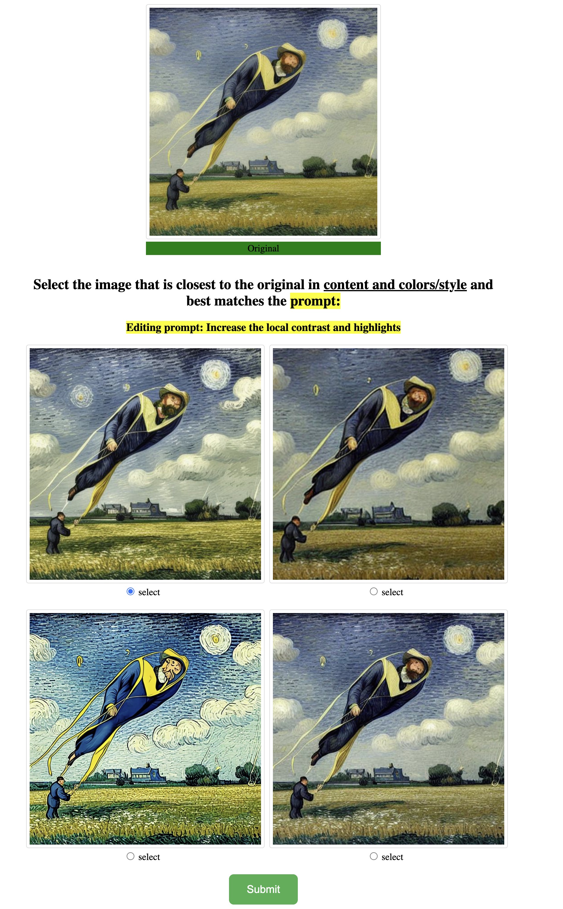
We conducted a user study comparing our method with instruction-based SD editing approaches, as no purely parametric alternatives are available. Specifically, we evaluated against InstructPix2Pix [brooksInstructPix2PixLearningFollow2023], InstructDiffusion (InstrDiff) [Geng23instructdiff], and StyleBooth [han2024stylebooth]. Using our test dataset (Sec.˜4.2), which includes 50 images generated with photographic and Van Gogh prompts, we produced results with each method for three different parameters by translating these parameters into prompts, trying out several variants and CfG settings and choosing those that best reflect our visual attribute dataset e.g., depth power parameter as “make it have an intense depth contrast and highlights." Participants were provided a brief explanation of the tasks, focusing on adherence to the editing prompt and maintaining the style and content of the original image. They were then presented with the original and four edited versions arranged in random order, asked to select their preferred result. We gathered 300 task samples from 50 participants revia prolific.com, with four responses per task. To filter ambiguous results, we retained tasks where at least three participants agreed on the preferred method, resulting in 235 usable samples. The results, shown in Tab.˜1, indicate that our method is generally preferred over the other approaches. In some cases, InstructPix2Pix produced more stable results for simpler tasks, such as darkening specific areas. We show a comparison for depth contrast in Fig.˜25, excluding InstrDiff[Geng23instructdiff] as its output failed to preserve the semantic content. More visual examples, details of the study and a screenshot of the study interface are provided in the supplemental material.
5.2 Quantitative
| Approach | LPIPS | Style | |
|---|---|---|---|
| Null Text Invers. [mokadyNULLTextInversionEditing] | 0.452 | 0.793 | 0.001 |
| Instruct Pix2Pix [brooksInstructPix2PixLearningFollow2023] | 0.259 | 0.907 | 0.007 |
| MagicBrush [zhang2024magicbrush] | 0.123 | 0.964 | 0.001 |
| InstructDiffusion [Geng23instructdiff] | 0.467 | 0.820 | 0.008 |
| Stylebooth [han2024stylebooth] | 0.597 | 0.817 | 0.004 |
| Ours | 0.343 | 0.894 | 0.001 |
Similarity metrics.
In Tab.˜2 we show similarity metrics in terms of perceptual (LPIPS), semantic (CLIP) and stylistic (NST [gatys2016image] style loss) similarity of editing methods to the original on our test dataset with the same editing captions as above. Following human–calibrated thresholds [zhang2018perceptual], LPIPS is typically imperceptible, whereas values denote major content change. We compute CLIP, the cosine similarity of OpenCLIP image embeddings [radford2021learningCLIP], which is found to capture human judgment of semantic scene similarity well ( human alignment for NIGHT [fu2023dreamsim] for OpenCLIP). From experimentation, values CLIPimg generally correspond to near-identity semantics, whereas the range would correspond to faithful but visibly edited images, and to a region where semantic drift is strong.
MagicBrush [zhang2024magicbrush] attains the highest CLIP but the lowest LPIPS, confirming that it largely leaves the image unchanged despite the prompt. Conversely, null-text inversion [mokadyNULLTextInversionEditing] shows the largest LPIPS and lowest CLIP evidencing over-editing artefacts. InstructPix2Pix [brooksInstructPix2PixLearningFollow2023] strikes a better trade-off but introduces the greatest stylistic drift, higher style scores typically indicate change in local textures and color - which would not be expected from the edits in our test dataset (e.g., Fig.˜25(d)). Our method yields a mid-high CLIP while keeping LPIPS and style loss inside the “visible-but-faithful” band, indicating salient yet well-integrated fine-stylistic edits that preserve the original semantics.
| Method | contour-width | depth-power | blackpoint |
|---|---|---|---|
| InstructPix2Pix | 33.4 | 49.7 | 51 |
| InstructDiffusion | 32.1 | 66.6 | 48.2 |
| StyleBooth | 16.6 | 18.5 | 17.5 |
| Ours | 9.3 | 14.9 | 13.7 |
Continuous control.
We compare the behaviour of state-of-the-art methods in adjusting stylization strength. Unlike our method, these methods approaches lack an explicit control parameter for stylization strength; instead, we adjust the text guidance scale of the editing prompt to approximate similar behavior. In Fig.˜24, we visualize the impact of increasing stylization strength by plotting LPIPS values against the unedited input images. Given the high diversity of samples, averaging LPIPS alone does not capture meaningful variations; hence, each thin line represents an individual input image incrementally stylized by increasing a single parameter’s strength. The graph demonstrates that our approach provides more consistent and predictable editing behavior compared to InstructPix2Pix, which displays abrupt jumps in LPIPS, making fine-grained stylization adjustments infeasible. Quantitatively, we measure smoothness using the ISTD metric [guo2024smooth] over the same set of generated images (increasing lambda or CfG). Compared to the methods in the user study, our approach significantly improves the ISTD. See supplemental for the plots for these methods.
6 Discussion
We presented a method for precise control of stylistic attributes in LDMs using stylistic control networks. By finetuning on datasets with stylistic effects applied at varying strengths, our approach learns disentangled editing directions mapped to explicit artistic control parameters. The guidance mechanism selectively amplifies the desired edits while suppressing irrelevant information and integrates seamlessly with the visual characteristics of the base Stable Diffusion model. This learning framework can reasonably be applied to any visual attribute parameterizable through a control setting.
Limitations
The stylistic control network adds runtime and memory consumption. Adding new stylistic controls requires additional training data, and parameter adjustments for strength and activation timesteps can lead to trade-offs between effect intensity and content preservation. Additionally, real image inversion and subsequent editing can introduce artifacts due to suboptimal inversions.
Our approach represents a step towards bridging the gap between traditional image editing and generative techniques. We believe it offers a promising direction for enhancing user control in image synthesis, providing a foundation for future research to further refine and expand the capabilities of LDMs in artistic and professional workflows.
References
Appendix
A Background
Diffusion models progressively add random noise to input data through a variance-preserving Markov process [sohl2015deep, ho2020denoising, song2020score]. They then learn to reverse this process by denoising, thereby generating the desired data samples. Latent Diffusion Models [rombach2022high] apply this process in a low-dimensional latent space , where a Variational Autoencoder (VAE) [kingma2013auto] first encodes an image into using a pretrained encoder and then noise is added to for timesteps until . During the denoising phase, the model predicts the noise delta at each timestep , moving from to . Here, is a neural network, often a U-Net [ronneberger2015u], and represents conditioning information, in our case text embeddings . The training loss in text-to-image models [rombach2022high] minimizes the difference between the actual noise and the predicted noise :
| (7) |
After the model is trained, it can effectively denoise from back to using an efficient diffusion sampler [song2020denoising, lu2022dpm].
Finally, the decoded image is reconstructed using a frozen decoder . The model is trained concurrently on both conditional () and unconditional (null-text embedding ) objectives. During inference, the difference between unconditioned and (text) conditioned outputs, denoted as vector , can guide the generative process towards the conditioned goal. This classifier-free guidance (CfG) [hojonathanClassifierFreeDiffusionGuidance2022] is computed as
| (8) | ||||
| (9) |
where, is the CfG scale that adjusts the intensity of the guidance.

B User Study Details
To apply the prompt-based editing methods to our testing dataset as described in Sec. 5.1, we use the following prompts (for the instruction based methods), and editing captions (shown to users):
-
[align=left]
-
depth power.
Prompt: “make it have an intense depth contrast and highlights". Editing description: “Increase the local contrast and highlights"
-
contour width.
Prompt: “make it have thick strokes". Editing description: “Increase the number and thickness of outlines in the image"
-
black point.
Prompt: “Lower the black point of the whole image". Editing description: “Lower the black point of the image"
To generate corresponding results with our method, we set for each parameter. In Fig.˜26 we plot response counts for the user study per style and parameter. Our method is preferred by a significant margin against all other methods for all parameters and styles, except for the blackpoint parameter with Van Gogh style. In Fig.˜33 we show samples from the study and in Fig.˜29 we show a screenshot from the web-interface of the user study.
C Additional Training Evaluation
We evaluated the impact of training steps and regularization on model performance, as shown in Fig.˜28. To measure visual differences, we used LPIPS [zhang2018perceptual] between images generated at and across various parameters. Increasing training steps amplifies the effect of on outputs, with structural changes like “contourWidth” showing greater visual impact than color or contrast adjustments like “depthPower” or “details.”
In Fig.˜30, we present additional outputs from the finetuned Controlnet alone (i.e., ), showing that training extra attention layers conditions model outputs on parameter-specific changes. Fig.˜27 compares model outputs at with algorithmic filtering on the same Controlnet-generated images . Using the same watercolor effect filters as in training, results indicate that higher regularization reduces similarity to algorithmic filtering. However, lower regularization values catch up after about 15k training steps, with similarities converging beyond this point. In Fig.˜32, we illustrate outputs across training steps and regularization settings for the depth power parameter. As with contour width (Fig.˜16), high regularization quickly reaches strong stylization, but excessive training may intensify stylization and alter content.

D Additional Results
In Fig.˜31, we show results for the artbench-finetuned model. In Fig.˜35, we vary both the activation timestep and parameter to show their respective influences. A higher (=later) activation step introduces less changes into the image, representing a tradeoff between stability of the image and strenghth of stylization. In Fig.˜34, we plot the stylization stability ( vs LPIPS) for all methods from our quantitative comparison. Notably, some text-based approaches exhibit minimal LPIPS change, indicating either limited sensitivity to text guidance scale or ineffective stylization even with increased guidance scale. Others display abrupt jumps in LPIPS, making fine-grained stylization adjustments infeasible.



Increase contours


Lower blackpoint


Increase depth contrast+highlights


