Analyticity and symmetry of band extrema in gapped solids: when does the effective mass approximation hold?
Abstract
The effective mass approximation is widely used across models of carrier transport, optical response, and excitons in semiconductors and insulators, but its validity hinges on the assumption that the band dispersion at the relevant extremum is analytic. We prove that analyticity holds at any non-degenerate extremum for the standard ab initio Hamiltonians, including density functional theory with local or hybrid exchange-correlation functionals and for band-edge quasiparticle energies in gapped systems. Band non-analyticity (or warping) in these settings is therefore intrinsically tied to degeneracy. We then use group theory to determine the symmetry-allowed form of the effective mass tensor for each of the 32 crystallographic point groups, providing a stringent consistency check on first-principles calculations. As a representative application, we show that the electron and hole effective masses at the point of monolayer MoS2 must be strictly isotropic at the DFT and levels.
I Introduction
The effective mass approximation is widely used in semiconductor physics as a simplified framework in which charge carriers in a periodic potential are described as free particles with a renormalized mass. Often, the effective mass is introduced via perturbation theory, under the implicit assumption that the band dispersion admits a convergent Taylor expansion at the extremum of interest. This assumption amounts to the requirement that is real-analytic near the relevant extremum, a requirement that has not been studied rigorously for the Hamiltonians actually used in modern ab initio calculations – density functional theory (DFT) with local or hybrid exchange-correlation functionals, Hartree–Fock, and . As a result, the validity of the effective mass approximation in standard first-principles practice is generally taken for granted rather than established rigorously. Once the validity of the effective mass approximation for a given extremum has been rigorously established, the symmetry-allowed form of the dispersion near the extremum is restricted not only by the inherent symmetry of the material, but also by the symmetry of second-order polynomials. These constraints together determine the number of independent components of the effective mass tensor, and the directions along which they are defined; yet anisotropy is frequently discussed phenomenologically in the first-principles literature, occasionally yielding reported tensors that are inconsistent with the symmetry of the crystal. Monolayer MoS2 provides a representative example: its -point conduction and valence bands are non-degenerate (apart from spin) and located at a symmetry point, which strictly forbids in-plane anisotropy of the effective mass, and yet anisotropic values have been reported [3, 9, 20].
This work addresses both the existence of a well-defined effective mass approximation and the symmetry constraints that it imposes. In Sec. II we state our main result on band analyticity (Theorem 1) and illustrate the relationship between band warping and degeneracy with a calculation on monolayer TiO2. In Section III we tabulate the symmetry-allowed form of the effective mass tensor for each of the 32 crystallographic point groups, and apply the classification to monolayer MoS2, where it also clarifies the origin of the anisotropies reported in the literature. In section IV we provide the proof of Theorem 1. Finally, in section V we summarize our results and discuss directions for future research.
II The effective mass approximation and band warping
flowchart
In the effective mass approximation, the band structure of a solid in the vicinity of a stationary point is expressed as
| (1) |
where the inverse effective mass tensor is defined as
| (2) |
and subscripts label the Cartesian components of the wavevector . Equation (1) presupposes that is twice differentiable at , so that the inverse effective mass tensor of Eq. (2) is well-defined, and that the right-hand side of Eq. (1) constitutes the leading non-trivial terms of a power series expansion of that converges to in a neighborhood of . The latter property is precisely the defining feature of an analytic function: is analytic at if it admits a power series expansion that converges to for sufficiently small. Since an analytic function is automatically infinitely differentiable, analyticity of at guarantees both requirements at once. The main result of the present work is the following theorem, which establishes such analyticity at non-degenerate extrema under conditions covering the most commonly employed approximations:
Theorem 1 - analyticity of non-degenerate bands
Let be a point in the Brillouin zone at which is non-degenerate. Then is a real-analytic function of in a neighborhood of in each of the following cases:
-
(i)
, where is a local potential (as in DFT with LDA, GGA, or meta-GGA exchange-correlation functionals).
-
(ii)
additionally contains a non-local potential whose kernel decays exponentially with . This includes, in particular, exact exchange in gapped systems (Hartree–Fock or hybrid DFT).
- (iii)
In particular, Eq. (1) is then the leading non-trivial term
of a convergent local power series representation of .
This conclusion is consistent with the numerical evidence reported in Ref. [18], that warping appears only in the presence of degeneracies. For such degenerate extrema, an expansion of the form (1) often does not exist; then fails to be analytic at , and the band is said to be warped. We use the terms warped and non-analytic interchangeably in the following.
For warped bands, Ref. [13] proposed the more general angular expansion
| (3) |
with and specifying the direction of . The function may be interpreted as a direction-dependent inverse mass, and Eq. (3) requires only one-dimensional analyticity of the band in at fixed . This form is therefore widely applicable, but generally harder to compute and use than the polynomial expansion (1), since accurate determination of requires fine angular sampling, and reducing it to a scalar effective mass requires an application-specific angular weighting that differs between transport coefficients [13, 12], density of states [14, 18], and other properties. When Eq. (1) applies, it is therefore preferable. This motivates the question of when, precisely, it does apply.
As an example of band warping, Fig. 2A shows the PBE band structure of monolayer TiO2. The valence band maximum occurs at the point and is doubly degenerate, leading to band warping in the vicinity of the degeneracy. This is shown in Fig. 2B where the two top valence bands are shown along a circle with radius Å-1 around the valence band maximum. If the bands had been analytic (non-warped), the four-fold rotational symmetry of the material would dictate a completely isotropic effective mass. The dispersion obtained by fitting the bands to Eq. (1) is shown by the dashed circles; it is evident that they do not describe the actual band dispersion, shown in blue and orange, very well. The degeneracy of the valence bands at may be lifted by applying a small strain of 0.1% along the -direction. This perturbation is so small that it has no visible effect on the band structure as shown in Fig. 2A. However, with the degeneracy lifted, the valence bands are now analytic at , and the effective mass approximation Eq. (1) perfectly describes the bands as shown by the dashed lines in Fig. 2C. We note that the strain lifts the degeneracy by reducing the 4-fold rotational symmetry to a 2-fold symmetry, thereby permitting anisotropy of the effective mass. This anisotropy is also evident in the bands in Fig. 2C.
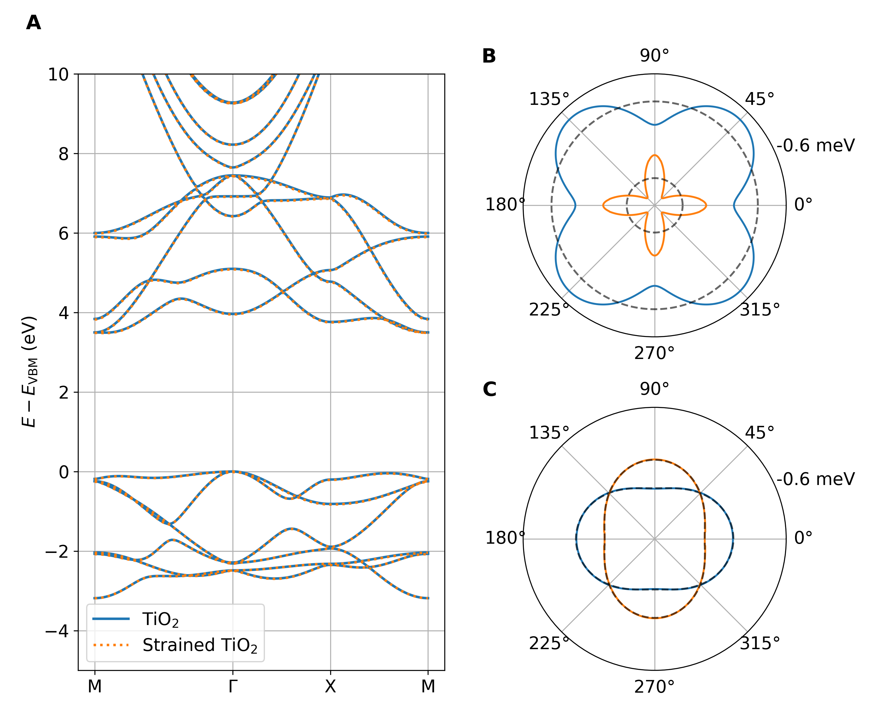
In Fig. 2, spin-orbit coupling (SOC) is not included, and spin-up and spin-down channels are therefore degenerate. However, in the absence of SOC, spin degeneracy is not enough to induce non-analyticity. Without SOC, the total electronic Hamiltonian may be written as a direct sum . Because the spin-up and spin-down sectors do not couple, theorem 1 may be applied to the two spin channels separately.
III Symmetry Constraints
As a physical observable, the band energy must remain invariant under all crystal symmetries. For three dimensions, these symmetries form a space group (in two dimensions, a layer group [6]). A symmetry operation acts in real space as , and in reciprocal space as , where is a point group operation and a translation. Invariance of the dispersion therefore requires
| (4) |
for any and any . For a fixed , the subset of operations that leave invariant up to a reciprocal lattice vector forms the little group . This group is isomorphic to one of the 32 crystallographic point groups (in both two and three dimensions). Writing , the effective mass approximation, Eq. (1), depends only on . For , Eq. (4) can be written
| (5) |
showing that the dispersion in the vicinity of is invariant under the action of any . In representation-theoretic language, the energy near transforms according to the totally symmetric (trivial) representation of . Since the effective mass surface is a quadratic form in , we can determine the symmetry-invariant terms by decomposing this quadratic form into the irreducible representations of the relevant point group.
Such a decomposition divides the 32 crystallographic point groups into three classes, as shown in table 1: in the cubic groups, the only quadratic form transforming according to the totally symmetric representation is . Consequently, for -points whose little group is cubic, the effective mass tensor is necessarily isotropic.
At the opposite extreme are the lowest-symmetry groups, containing at most a 2-fold rotational axis. In these, the monomials and independently transform according to the trivial representation. Any linear combination of them is therefore symmetry-allowed, and the effective-mass tensor may be fully anisotropic with three independent principal components. The remaining groups form an intermediate class. Here, the trivial representation is spanned by and . This dictates uniaxial symmetry, i.e. the existence of an axis such that the mass is isotropic within the plane perpendicular to the axis, but distinct along the axis. This category includes all the non-cubic groups with an -fold rotation axis with , and is the largest of the three classes. These conclusions all hold both with or without SOC; although spinor states acquire a sign change under rotation by , the band energy is always invariant. The symmetry constraints on the effective mass tensor therefore depend only on the ordinary point group .
| Fully Isotropic | |
|---|---|
| Uniaxially Isotropic | |
| Anisotropic |
These symmetry constraints provide a rigorous consistency check for first-principles calculations. As an example of their consequence, we study the electron- and hole effective masses of monolayer MoS2 calculated using the finite-difference method at the PBE level. Monolayer MoS2 is a direct gap semiconductor with valence band maximum (VBM) and conduction band minimum (CBM) both located at the -point of the Brillouin zone. These bands are both non-degenerate at the extrema (apart from a trivial spin-degeneracy), and therefore the bands must be analytic at the PBE level according to theorem 1. The effective mass approximation (1) therefore applies.
The little group of is isomorphic to , which according to table 1 signifies a uniaxially isotropic effective mass. There are therefore two independent directions for the effective mass - in-plane and out-of-plane components; and since we are dealing with a two-dimensional material, there is no concept of an out-of-plane effective mass. Therefore, the effective mass is fully isotropic. This conclusion stands in contrast to several reported calculations for monolayer MoS2, which find different effective masses along the and directions or describe them as almost isotropic [3, 9, 20]. As we now show, this apparent anisotropy is likely a numerical artifact of the finite-difference scheme. Figure 3 shows the electron and hole effective masses of monolayer MoS2 calculated in the finite-difference scheme without SOC. The effective mass has been calculated both in the K and KM directions. As the step size is reduced, the effective mass converges to the same value regardless of the direction the limit is taken, showing that the effective mass is indeed isotropic. For larger step sizes, cubic and quartic terms in the dispersion introduce spurious anisotropy. Due to the geometry of the Brillouin zone, shown in the inset of Fig. 3, the direction is equivalent to , which is exactly the opposite direction as . This means that cubic terms in the dispersion contribute with opposite signs in the and directions, making this class of material particularly sensitive to step size convergence in the determination of the effective mass.

IV Proof of Theorem 1.
In a periodic system, the electronic eigenstates take the form of Bloch states , where the functions have the periodicity of the lattice, i.e. for any lattice vector , . This allows us to define the Bloch Hamiltonian from the relation
| (6) |
where may be any Bloch-like function in the domain of , i.e. it is not necessarily an eigenstate of . The real-space kernel of the Hamiltonian in Eq. (6) can be expressed as
| (7) |
If does not contain any non-local potentials, only the term contributes, and we find the well-known result
| (8) |
This is explicitly a polynomial in and therefore analytic; in particular, as the domain of is independent of , Eq. (8) defines an analytic family of operators of type (A) [10], the most restrictive class. A direct consequence is that non-degenerate eigenvalues and eigenfunctions of are analytic in , and we therefore have nothing more to prove in this important case, which among other models covers DFT Hamiltonians with local potentials, i.e. LDA, GGA and meta-GGA approximations.
For Hamiltonians with non-local interactions, analyticity depends on the convergence of the sum (7). In particular, the Weierstrass theorem [1] guarantees that if the sum converges uniformly then is analytic in . Since the non-local terms constitute a bounded perturbation of , the full Hamiltonian remains an analytic family of type (A). We remind the reader that a series is said to be uniformly convergent if for all there exists an such that for all and all ,
An important example of this type is the case of exact exchange, where the Hamiltonian contains a non-local term . Here is the Coulomb interaction and
| (9) |
is the single-particle density matrix of the system. For gapped materials (i.e. insulators and semiconductors) the density matrix decays exponentially with for large . This may be seen as a consequence of the principle of nearsightedness of electronic matter [11, 15]. To be precise, exponential decay means that there exists positive constants and such that
| (10) |
for all satisfying . It can be straightforwardly verified that such exponential decay is sufficient to guarantee uniform convergence of Eq. (7). While the exchange interaction is the most commonly encountered non-local interaction, we note that the above argument holds for any non-local potential which satisfies a bound of the type Eq. (10).
IV.1 Quasiparticle energies in
In many-body perturbation theory, the quasiparticle (QP) energies are roots of the nonlinear equation
| (11) |
where is the many-body self-energy. In standard practice, Eq. (11) is linearized around the Kohn–Sham eigenvalue [8, 17, 2], giving the explicit formula
| (12) |
with the QP renormalization factor
| (13) |
When is found from the linearized Eq. (12), it is analytic wherever and are. In the previous section, we established sufficient conditions for the single-particle energy to be analytic in . It remains to be shown that is analytic in at . This is established in Sec. IV.2. We note that Eq. (12) is only meaningful if is finite, i.e. the QP picture is valid. We assume this in the following, and note that analyticity of in automatically implies analyticity of wherever the latter is finite.
It is also possible to solve the nonlinear QP equation (11) directly rather than by linearization, which may sometimes result in better QP energies [16]. In this case, we can establish analyticity via the implicit function theorem (IFT) [10]. Writing
| (14) |
the QP equation (11) amounts to . The IFT guarantees that the locus of this equation implicitly defines an analytic function under the conditions that is analytic in at and that
| (15) |
As in the linearized case, analyticity of reduces to analyticity of in at the relevant energy; here, however, that energy is the QP energy itself rather than . As we will show in the next section, this requirement is fulfilled if
| (16) |
which is typically satisfied in practice.
IV.2 Analyticity of the self-energy
The time-ordered self-energy which enters in the quasi-particle equation is
| (17) |
where
| (18) |
is the single-particle Green’s function, and the screened Coulomb interaction. Introducing in the same manner as of Eq. (6), we obtain a Fourier-like series
| (19) |
where
| (20) |
If the single-particle Hamiltonian is analytic in , as discussed in the previous section, and is non-degenerate, then the wavefunction is locally analytic in [10]. Each is analytic in as it is defined from a finite-volume integral of functions that are analytic in . We now examine the conditions under which decays exponentially with ; as noted in the previous section, this condition is sufficient for the sum (19) to define an analytic function by the Weierstrass theorem.
We focus on the correlation part of the self-energy, where , because the exchange part is already known to be exponentially localized due to the previously discussed localization of the density matrix in gapped systems. The correlation self-energy may be obtained from Eq. (17) by simply replacing by . To proceed, we seek a formal spectral representation of . This can be achieved by noting that admits the general spectral representation [7]
| (21) |
where the poles correspond to neutral excitation energies. Combining Eqs. (17), (18) and (21), we arrive at the spectral representation of [5]:
| (22) | |||
We note that has poles at for occupied states and at for unoccupied states . Since the are strictly positive, this defines a strip
| (23) |
around the band gap in which is analytic, as illustrated in Fig. 4. If is calculated in the RPA, the are bounded below by the KS gap, so the strip is at least as wide as .

In Appendix A we show how can be represented in terms of the resolvents of two families of auxiliary operators . Using this representation we demonstrate via the Combes–Thomas estimate [4] that is exponentially localized in for . As in the case of exact exchange, this localization guarantees uniform convergence of the series (19), and by the Weierstrass theorem, analyticity of in both and for whenever is non-degenerate. Since lies in for any band-edge state of a gapped system, the explicit linearized formula (12) establishes analyticity of in directly. If the nonlinear QP equation (11) is used, analyticity holds if . When is calculated in the RPA, as typically done, this guarantees analycity as long as the QP correction is smaller than the gap, i.e. Eq. (16). The effective mass approximation therefore holds at non-degenerate band edges of gapped semiconductors and insulators at the level as long as the calculation is based on a single-particle Hamiltonian satisyfing either cases (i) or (ii) of Theorem 1. We note that the analyticity applies to all non-degenerate bands whose energy lies within the strip . This distinguishes from case (ii) of Theorem 1, where all non-degenerate bands are analytic.
V Conclusion
We have established conditions under which the effective mass approximation, Eq. (1), is rigorously valid at non-degenerate band extrema in semiconductors and insulators. Specifically, is analytic at any point where it is non-degenerate for the standard mean-field Hamiltonians (DFT with local exchange-correlation potentials, Hartree–Fock, and hybrid DFT). The same applies to non-degenerate band energies of gapped systems at the level when is evaluated within the strip surrounding the gap. If the linearized QP equation (12) is used, this condition is always satisfied at the band edges. In contrast, if the nonlinear QP equation (11) is used, an additional condition is necessary.
This implies that band warping at a non-degenerate extremum is impossible in these settings, so warping is intrinsically tied to degeneracy.
For analytic extrema, the symmetry-allowed form of the effective mass tensor is fully determined by the little group of , and the decomposition of quadratic forms into its irreducible representations yields three classes of materials which permit different degrees of effective mass anisotropy. These findings are summarized in Table 1, and provide a stringent consistency check for first-principles calculations.
Several extensions of the present results would be of interest. The proof does not extend straightforwardly to the self-consistent variants of . In eigenvalue self-consistent [17] (ev) and QP self-consistent [19] (qs), self-consistency is obtained via the construction of a modified single-particle Hamiltonian (explicitly in qs; implicitly in ev). These auxiliary Hamiltonians may not be exponentially localized, even if the initial is, and our proof of analyticity of therefore does not apply. In fully self-consistent (sc), by contrast, the Green’s function is no longer the resolvent of any single-particle Hamiltonian, and the spectral representation of underlying our localization argument is therefore invalidated.
Finally, degenerate extrema are known to be sometimes – but not always – warped, and the conditions distinguishing the two cases would benefit from a similarly systematic treatment.
Acknowledgments
The authors would like to thank Jan Philip Solovej for providing helpful comments on an earlier version of the manuscript. The authors acknowledge funding from the Villum Investigator Grant No. 37789 supported by VILLUM FONDEN and from the Novo Nordisk Foundation Data Science Research Infrastructure 2022 Grant (NNF22OC0078009).
Appendix A Representation of from resolvents of two auxiliary operators
Using the projector into the occupied subspace , whose real-space representation is the density matrix , we now introduce two families of operators given by
| (24) |
and
| (25) |
where and are arbitrary constants. We wish to show that can be written in terms of the resolvents . These have the form
| (26) |
and
| (27) |
which may be seen from the identity , which can be verified to hold on the occupied and unoccupied subspaces independently. From Eqs. (26) and (27), the spectral representation of can be written
| (28) | |||
The shifts are gauge parameters: they fix the eigenvalues of on the unoccupied/occupied subspaces to , and the corresponding poles of cancel exactly against the subtracted terms in Eq. (28). Hence is independent of and , and has no pole inside the gap. We now take , so that resolvents are bounded on all of .
In Appendix B, we show that the Combes–Thomas estimate [4] can be applied to the operators . For , this implies that the resolvents are exponentially localized; precisely, this means that the localized operator norm decays exponentially in for sufficiently large, where and are characteristic functions of unit cells at the origin and at lattice vector , respectively. Such localized matrix elements are precisely what enters in the definition of the in Eq. (20). Since and enter Eq. (28) as local multiplicative prefactors, the exponential decay carries over to .
Appendix B Combes–Thomas estimate for non-local Hamiltonians
We show that the operators of Eqs. (24–25) have resolvents whose matrix elements between spatially separated unit cells decay exponentially with the separation. Let and denote unit cells centered at the origin and at a lattice vector respectively, and let and be the corresponding characteristic functions, i.e.
| (29) |
We wish to establish bounds of the form
| (30) |
for constants , outside the spectrum of , and sufficiently large. The bound (30) is the key needed to establish analyticity of the self-energy in Eq. (19) since the terms in the sum are matrix elements of between functions localized in the unit cells and . The estimate (30) therefore implies for large , which guarantees uniform convergence of the lattice sum and thus analyticity of the self-energy in .
We first prove the estimate for bounded operators with exponentially decaying kernels. In general, however, the Hamiltonian of an electronic system is unbounded due to the Laplacian in the kinetic energy term. We therefore extend the argument to Schrödinger-like Hamiltonians that may contain an additional bounded, non-local (but exponentially decaying) potential.
The two operators require different treatments. The operator of Eq. (24) is bounded due to the projection into the occupied subspace. On the other hand, (Eq. (25)) can be written
| (31) |
i.e. a shifted Kohn–Sham Hamiltonian plus a bounded perturbation, and is treated by the unbounded-operator extension in the following.
Bounded operators
Let be a bounded operator with an exponentially decaying kernel, i.e. for larger than some . We denote the resolvent .
Following the standard Combes–Thomas approach, we define for a unit vector and , and the conjugated operator . Using the identity , the resolvent of can be written
| (32) |
Inserting characteristic functions and on either side and taking operator norms, we find
| (33) |
The operators and are multiplicative operators restricted to bounded domains, and are therefore bounded. Their norms depend on the direction . We choose with and define . For , the norm is then . For , we can similarly bound . Using these bounds in Eq. (33), we obtain
| (34) |
where . For much larger than the cell size , this gives the desired exponential decay in . However, the above argument works only provided the conjugated resolvent exists and is bounded. We now show that for sufficiently small , this is indeed the case.
The so-called Schur test bounds the norm of an operator by integrals of its matrix elements, namely
| (35) |
Consider the matrix elements of ,
For , the exponential decay of means that the matrix elements of decay as , which is integrable for . Meanwhile, the region where is finite in size, and the integral is therefore finite as long as contains no non-integrable singularities, which is true of the operators in the main text. From these considerations, it can be immediately verified that the Schur test guarantees that as .
The resolvent of can be written
For in the resolvent set of , is bounded. We now choose sufficiently small such that . Then, we may write
| (36) |
where the bound on the operator norm of the terms in the sum guarantees convergence of the series, and therefore establishes that the left-hand side is bounded. This shows that for sufficiently small and in the resolvent set of , exists and is bounded. This completes the proof of (30).
Unbounded Hamiltonians with non-local potentials
We now extend the estimate to unbounded operators of the form
| (37) |
where is the Laplacian, is a local potential, and is a non-local but exponentially decaying potential, i.e. for sufficiently large. For our application, falls into this framework with
The structure of the proof is the same: we conjugate by and show that the conjugated resolvent remains bounded for small enough . The bound (30) then follows from the same factorization as in Eq. (33).
The perturbation decomposes as
| (38) |
Consider first the local part. Since commutes with , the perturbation acts only on the kinetic energy,
| (39) |
so . Since is relatively bounded with respect to (and hence with respect to ), for any in the domain of , we have
| (40) |
where and are constants such that . This is the standard step in the Combes–Thomas argument for Schrödinger operators and does not require to be bounded [4].
The non-local part has the same structure as in the bounded case, with kernel . Since is bounded with an exponentially decaying kernel, the Schur test gives as for .
As in the previous section, we may write
| (41) |
where . The right-hand side exists and is bounded when . By the triangle inequality,
| (42) | ||||
For the first term, since is in the resolvent set, maps into the domain of and the relative bound (40) applies. Using , we find
| (43) | |||
which vanishes as . The second term in (42) likewise vanishes since . We conclude that for sufficiently small , the resolvent is bounded. This completes the proof.
References
- [1] (1979) Complex analysis. Vol. 3, McGraw-Hill New York. Cited by: §IV.
- [2] (1998) The gw method. Reports on progress in Physics 61 (3), pp. 237–312. Cited by: §IV.1.
- [3] (2012) Quasiparticle band structure calculation of monolayer, bilayer, and bulk mos 2. Physical Review B—Condensed Matter and Materials Physics 85 (20), pp. 205302. Cited by: §I, §III.
- [4] (1973) Asymptotic behaviour of eigenfunctions for multiparticle schrödinger operators. Communications in Mathematical Physics 34, pp. 251–270. Cited by: Appendix A, Appendix B, §IV.2.
- [5] (2020) Robust analytic-continuation approach to many-body gw calculations. Journal of Chemical Theory and Computation 16 (3), pp. 1742–1756. Cited by: §IV.2.
- [6] (2024) Symmetry classification of 2d materials: layer groups versus space groups. 2D Materials 11 (3), pp. 035009. Cited by: §III.
- [7] (2019) GW quasiparticle energies of atoms in strong magnetic fields. The Journal of Chemical Physics 150 (21). Cited by: §IV.2.
- [8] (1986) Electron correlation in semiconductors and insulators: band gaps and quasiparticle energies. Physical Review B 34 (8), pp. 5390. Cited by: §IV.1.
- [9] (2012) Electronic structure of a single mos2 monolayer. Solid state communications 152 (10), pp. 909–913. Cited by: §I, §III.
- [10] (2013) Perturbation theory for linear operators. Springer. Cited by: §IV.1, §IV.2, §IV.
- [11] (1996) Density functional and density matrix method scaling linearly with the number of atoms. Physical Review Letters 76 (17), pp. 3168. Cited by: §IV.
- [12] (2016) Precise effective masses from density functional perturbation theory. Physical Review B 93 (20), pp. 205147. Cited by: §II.
- [13] (2014) Theory of band warping and its effects on thermoelectronic transport properties. Physical Review B 89 (15), pp. 155131. Cited by: §II, §II.
- [14] (2016) Density of states for warped energy bands. Scientific Reports 6 (1), pp. 22098. Cited by: §II.
- [15] (2005) Nearsightedness of electronic matter. Proceedings of the National Academy of Sciences 102 (33), pp. 11635–11638. Cited by: §IV.
- [16] (2021) Towards fully automated gw band structure calculations: what we can learn from 60.000 self-energy evaluations. npj Computational Materials 7 (1), pp. 22. Cited by: §IV.1.
- [17] (2007) Self-consistent gw calculations for semiconductors and insulators. Physical Review B—Condensed Matter and Materials Physics 75 (23), pp. 235102. Cited by: §IV.1, §V.
- [18] (2022) Two-layer high-throughput: effective mass calculations including warping. Engineering 10 (3), pp. 74–80. Cited by: §II, §II.
- [19] (2006) Quasiparticle self-consistent gw theory. Physical review letters 96 (22), pp. 226402. Cited by: §V.
- [20] (2014) Tunable electronic properties of two-dimensional transition metal dichalcogenide alloys: a first-principles prediction. The journal of physical chemistry letters 5 (2), pp. 285–291. Cited by: §I, §III.