Computer Science Institute of Charles University, Prague, Czech Republic babak@iuuk.mff.cuni.cz Supported by grant 25-16627S of the Czech Science Foundation. Computer Science Institute of Charles University, Prague, Czech Republic samal@iuuk.mff.cuni.cz Supported by grant 25-16627S of the Czech Science Foundation. \CopyrightBabak Ghanbari and Robert Šámal
Acknowledgements.
We thank Matt DeVos for helpful discussion.A Near-Linear-Time Algorithm for Finding a Well-Spread Perfect Matching in Bridgeless Cubic Graphs
Abstract
We present a near-linear-time algorithm that, given a bridgeless cubic graph, finds a perfect matching intersecting every 3-edge-cut in exactly one edge. This improves over a cubic algorithm of Boyd et al. for the same problem, and over our previous algorithm, which worked only for 3-edge-connected graphs. The main ingredient is a cactus representation of the 2-edge-cuts, together with an efficient update procedure under 2-cut reductions.
keywords:
bridgeless cubic graphs, well-spread perfect matching, edge cuts, cactus representationcategory:
\relatedversion1 Introduction
It is well known [JuliusPetersen] that every bridgeless cubic (i.e., 3-regular) graph has a perfect matching. Edmonds [Edmonds_1965] was the first to give a polynomial-time algorithm for finding a perfect matching (in any graph admitting one). The best algorithm for finding a perfect matching in bridgeless cubic graphs is currently due to Diks and Stańczyk [Diks] with time complexity of .
Less well known is the fact that a bridgeless cubic graph has a perfect matching that does not contain any 3-edge-cut entirely: If is a set of three edges forming a minimal edge-cut, then every perfect matching satisfies or . There exists a perfect matching for which this intersection has size for every 3-edge-cut ; we call such a matching a well-spread perfect matching, or WSPM for short. The existence of a WSPM was proved by Kaiser, Král’ and Norine [Kaiser] (and used to study how large fraction of the edge set can be covered by two, three, etc. perfect matchings).
A completely different motivation for the same question was given by Boyd, Iwata and Takazawa [boyd]. Their focus is on the complement of the perfect matching—a 2-factor in the given graph that intersects every 3-edge-cut. They provide a polynomial-time algorithm to find such a 2-factor and point out that a Hamiltonian cycle is also such a 2-factor. Thus, their result can be understood as an approximation approach to find Hamiltonian cycle (TSP tours) in cubic graphs—an NP-complete problem and, indeed, such a cycle need not exist in a cubic bridgeless graph. They also showed that their algorithm helps to achieve a better approximation algorithm for a smallest 2-edge-connected subgraph.
In our previous paper [GS25] we improved the algorithm of Boyd et al. to time , but with a significant limitation: our algorithm only worked on 3-edge-connected graphs. Indeed, the main idea in that paper was to use a tree representation of all 3-edge-cuts and efficiently update it. In this paper we remove this limitation and present an algorithm to find a WSPM in any bridgeless cubic graph. (For graphs with bridges, no perfect matching may exist at all, let alone well-spread one.) The challenge is that in the presence of 2-edge-cuts, the 3-edge-cuts no longer have a tree-like structure and even their number can be exponential. Also, the structure of 2-edge-cuts is more complicated than the structure of 3-edge-cuts in a 3-edge-connected graph.
The algorithm uses a prescribed-edge version of the 3-edge-connected algorithm: in a 3-edge-connected cubic graph, we can find a WSPM either containing or avoiding a specified edge. This allows the matchings of the reduced pieces to be glued consistently. In addition, we use the cactus representation of 2-edge-cuts (and its efficient update) to deal with the general case. The main technical contribution of the present paper is to show that the cactus representation can be updated throughout the reduction process while preserving enough information to glue prescribed well-spread perfect matchings in the pieces. The main result we obtain in this paper is the following:
Theorem 1.1.
Algorithm 1 returns a well-spread perfect matching in a bridgeless cubic graph on vertices in time .
This also strengthens our result from [Ghanbari]: the famous Cycle Double Cover conjecture [szekeres_1973, seymour1979sums] says (in one equivalent formulation) that every bridgeless cubic graph has a surface embedding with no singular edges (edges with the same face on both sides). We can find an approximation of this: an embedding with at most singular edges. We can do this in near-linear time, now for any bridgeless cubic graph.
2 2-edge-cuts
Graphs may have parallel edges but no loops; a graph in which every vertex has degree is called cubic. A cycle is a connected -regular graph. A bridge in a graph is an edge whose removal increases the number of connected components of ; equivalently, it is an edge that is not contained in any cycle of . A graph is bridgeless if it contains no bridges. A connected graph is -edge-connected if it remains connected after the removal of any set of fewer than edges.
Let be a bridgeless graph. Two edges and are called equivalent, written , if or is a -edge-cut of . If , then for every cycle of , we have if and only if . In particular, is an equivalence relation on .
The following lemma is straightforward and well-known.
Lemma 2.1.
Let be a bridgeless cubic graph. If , then for every perfect matching of , either both and belong to , or neither of them does.
A well-spread perfect matching in a bridgeless cubic graph is a perfect matching that contains exactly one edge from each -edge-cut of . A -edge-cut is an inclusion-minimal edge cut of size , that is a set of edges whose removal increases the number of connected components of and each of them is needed.
Let be a -edge-cut where , . We define a -cut reduction (more specifically, -reduction) of a graph as follows. Construct a bridgeless cubic graph from by removing and and adding two new edges and to the edges of . Then, and . Therefore, if and are the components of with and , then is a -cut reduction of . See the following figure.
![[Uncaptioned image]](2605.00710v1/2-cut-reduction.png)
Lemma 2.2.
A -cut reduction of a bridgeless cubic graph is again a bridgeless cubic graph.
Proof 2.3.
Let be a bridgeless cubic graph and let be a -edge-cut, where , Let have components and such that and . The -cut reduction replaces and with and , and the resulting graph is . Since is cubic, every vertex has degree . Removing and decreases the degree of each of by . Adding increases the degree of and by , and adding increases the degree of and by . All other vertices are unchanged. Hence every vertex of has degree , so is cubic.
Now we show that no edge of is a bridge. First consider any original edge of (the same argument applies to ). If were a bridge of , then it would also be a bridge of . We will show that it would also be a bridge of . Any path in connecting the two sides of either stays in , or enters through one of and returns through the other. The former is impossible as we are assuming is a bridge in . In the latter case, the subpath through can be replaced by the new edge . Hence such a path would also exist in , contradicting that is a bridge there.
It remains to show that the new edges and are not bridges. Since is bridgeless, the edge lies on a cycle in . Because is a -edge-cut, any cycle containing must also contain . Removing and from leaves a – path entirely in and a – path entirely in . Adding closes the path in to form a cycle containing , and adding closes the path in to form a cycle containing . Therefore, both and lie on cycles in and are not bridges.
Lemma 2.4.
Let be a bridgeless graph and let and , and be -edge-cuts in . Perform the -reduction of , and let be the component of the resulting graph that contains . Let be the new edge added to by the reduction. Then is a -edge-cut in .
Proof 2.5.
Let , , and . Let be the connected component of containing and , let be the connected component of containing and , and let be the connected component of containing and (see Figure 1).
Since is a -edge-cut, the graph has two components. In the -reduction, the component containing receives a new edge , while the other component receives a new edge . Let be the component containing .
Suppose that is not a -edge-cut in . Then there exists a – path in . The path avoids the new edge and also avoids . Therefore, is a – path in .
By the definition of , there exists a – path in , a – path in , and a – path in . Note that a – path exists otherwise is a bridge. Each of the paths avoids the edges and by construction, and avoids by assumption. Now the concatenation is a – path in . This contradicts the fact that is a -edge-cut of . Therefore is a -edge-cut in .

Lemma 2.6.
Let be a graph, and be a 2-edge-cut in . Suppose that , , and form a 3-edge-cut in . Then , , and form a 3-edge-cut in as well.
Proof 2.7.
Let , , and . Let and be the components of where . Suppose that is not a 3-edge-cut. Then, there exists a – path in . Since only are the edges between and and both ends of are in , the path cannot use . Therefore, is also a – path in . This is a contradiction to being a 2-edge-cut.
The following theorem is the main tool to reduce the problem to that for 3-edge-connected graphs. The proof is somewhat tedious, so we provide it in the appendix.
Theorem 2.8.
Let be a bridgeless cubic graph and let be a -edge-cut of . Let and be the graphs obtained from the corresponding -cut reduction, and let and be the new edges created by the reduction. Let and be well-spread perfect matchings of and that agree on and . Then has a well-spread perfect matching , that we call a gluing of and . Moreover, can be obtained efficiently: it equals or depending on whether .
3 Cactus representation of 2-cuts
Recall that for a connected graph and a nonempty proper subset , the set is called an edge cut of . A minimum cut of is an edge cut of minimum size. The edge-connectivity is the size of a minimum cut, and the local edge-connectivity of two vertices , is the size of a smallest edge cut disconnecting from . An inclusion-wise maximal subset such that for all is called a -edge-connected component of .
Let denote the set of all minimum cuts of . A cactus is a connected graph in which each edge is contained in at most one cycle. We allow 2-cycles but not loops.
For cacti in which every cycle has length at least , it is known [west2001introduction, P.160] that the number of edges is at most . However, this bound does not apply in our setting, since we allow -cycles. Allowing -cycles increases the maximum possible number of edges: the extremal example is obtained by taking copies of a -cycle sharing a single common vertex. We therefore use the following observation.
Let be a cactus with vertices, where -cycles are allowed but loops are not. Then .
Definition 3.1.
Let be a graph and be a cactus. A pair with is called a cactus representation (or cactus model) for the graph if it meets the following criteria:
-
1.
For every minimum cut , the cut in defined by , and is a minimum cut in .
-
2.
Conversely, for every minimum cut in , there exists a minimum cut
such that , and .
Let be a bridgeless graph with at least one -edge-cut. After contracting each -edge-connected component of to a single node, one obtains a cactus representing all 2-edge-cuts of [Nagamochi, Section 2.3]. In this case, the nodes of correspond to the -edge-connected components of , and no empty nodes are needed [Nagamochi, Section 2.3.5]. Note that the sets form a partition of , but a node need not correspond to an induced subgraph that is itself -edge-connected. Moreover, for two edges joining distinct contracted components, the pair forms a -edge-cut in if and only if the corresponding edges of lie on a common cycle [Nagamochi] (see Figure 2).
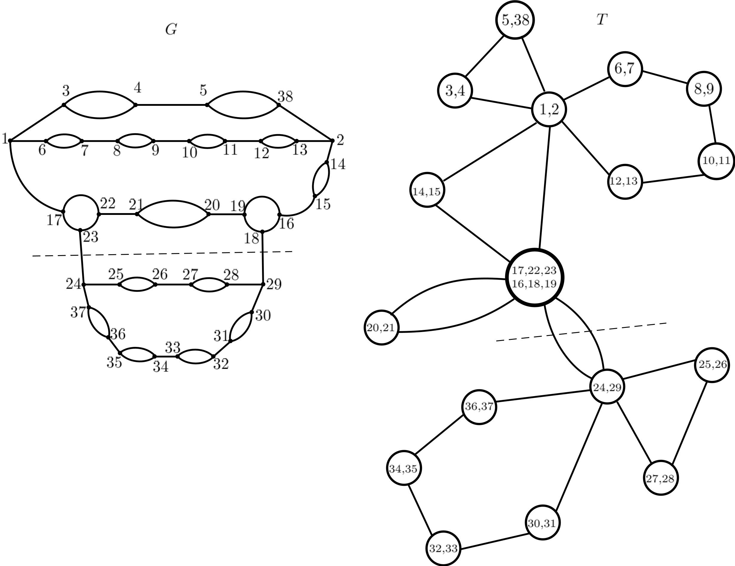
For a mapping , an edge is called external if .
Lemma 3.2.
Let be a bridgeless cubic graph with at least one -edge-cut and let be a cactus representation of all -edge-cuts of . Let be a -edge-cut of , and let be the corresponding -edge-cut in . Perform the -reduction in , obtaining graphs and with new edges and . Perform the -reduction in , obtaining graphs and . If a loop is created in or , delete it. Then and are cactus representations of all -edge-cuts of and , respectively.
Proof 3.3.
We prove the statement for ; the proof for is symmetric.
Let be the components of , so that and , where and are the new edges. Let be the components of , and let and be the new edges added to and , respectively, by the -reduction. Delete or if it is a loop.
By Lemma 2.2, is bridgeless cubic, so its minimum cuts are exactly its -edge-cuts. Thus it suffices to show that for any external edges of , the pair forms a -edge-cut in if and only if the corresponding edges of lie on a common cycle.
Case 1: . Then . We claim that is a -edge-cut in if and only if is a -edge-cut in . Indeed, any path in that traverses must enter through one of and leave through the other, so each maximal subpath through can be replaced by the single edge , yielding a path in . Conversely, any use of in a path of can be expanded to a path through , then inside , and then through , yielding a path in . Hence the claim follows.
Since is a cactus representation of all -edge-cuts of , the latter is equivalent to the corresponding edges of lying on a common cycle. As neither corresponding edge is or , this is equivalent to the corresponding edges in lying on a common cycle. Therefore is a -edge-cut in if and only if the corresponding edges lie on a common cycle in .
Case 2: one edge is , say . Let be the edge of corresponding to . Assume first that and lie on a common cycle in . Then the edge of corresponding to lies on the cycle containing and . Since represents all -edge-cuts of , both and are -edge-cuts in . By Lemma 2.4, after performing the -reduction, it follows that is a -edge-cut in .
Conversely, assume that is a -edge-cut in . We show that is a -edge-cut in . Suppose not. Then there exists in a path joining the two ends of . Since is a -edge-cut, every such path must use , and its subpath inside yields a path in joining the ends of , a contradiction. Hence is a -edge-cut in . Since is also a -edge-cut, the corresponding edge of lies on the same cycle as and , and therefore lies on a common cycle with in .
Thus also in this case is a -edge-cut in if and only if the corresponding edges lie on a common cycle in .
Finally, if is a loop, we delete it. This does not affect the set of represented -edge-cuts, since a loop belongs to no cycle of the cactus. Therefore is a cactus representation of all -edge-cuts of . The proof for is identical.

Theorem 3.4.
Let be a -edge-connected cubic graph and let . Then there exists a well-spread perfect matching such that . Moreover, such a matching can be computed in time .
Proof 3.5.
Let . We use Algorithm 1 from [GS25]. Let be the tree representation of the nontrivial 3-edge-cuts. Since is -edge-connected and cubic, every vertex of is mapped to a leaf of . In particular, both and are leaves of . Let be the unique neighbour of the leaf , and root at .
Consider the decomposition phase of Algorithm 1 of [GS25]. At each step, the algorithm separates a graph corresponding to a non-root subtree of . Since is a leaf whose parent is the root , no separated subtree contains (the subtree consisting solely of is processed only at the final step). Hence no separated graph contains the vertex . Therefore, no separated graph can contain the whole edge , because that would require it to contain both endpoints of . Consequently, the edge remains present in the current graph throughout the decomposition phase. In particular, it is present in the final graph associated with the root . At the end of the decomposition phase, the remaining graph (the graph associated with the root ) has no non-trivial -edge-cuts, and hence is internally -edge-connected (see [GS25]). In particular, is a bridgeless cubic graph. By Theorem 1 of [GS25] (Schönberger’s theorem), there exists a perfect matching of that contains the edge , and such a matching can be found in time .
We now perform the assembly phase of Algorithm 1 of [GS25]. At each step, we combine the current matching with a perfect matching of a previously separated graph using Theorem 2 of [GS25]. Since all matchings agree on the corresponding -edge-cuts, the resulting matching remains perfect and well-spread. Since was present in and was chosen to belong to , and the assembly procedure never removes edges from the current matching, it follows that , where is the final matching obtained for . The running time is the same as in Algorithm 1 of [GS25], which is . Thus, there exists a well-spread perfect matching of containing , and it can be found in time .
Corollary 3.6.
Let be a -edge-connected cubic graph and let . Then there exists a well-spread perfect matching such that . Moreover, such a matching can be computed in time .
Proof 3.7.
Let and be two edges in incident at . By Theorem 3.4 there exists a well-spread perfect matching such that . Since is already covered by , .
4 Algorithm
At each step we choose a vertex of degree in the cactus. (It exists, unless there is no 2-edge-cut left, as follows easily by Observation 3.) The two cactus edges incident with this vertex correspond to a -edge-cut in the current graph. Performing the corresponding -cut reduction separates a -edge-connected graph from the remainder. Repeating this procedure gives a sequence together with -edge-connected graphs where for each the graph is reduced along a -edge-cut into two graphs and (for ), and in the final step the graph is reduced into two -edge-connected graphs and .
To achieve the required running time, we store the graph and the cactus using adjacency lists and maintain the list of degree-2 nodes of the cactus. For each cactus node we store the list of vertices . For each cactus edge we store the corresponding external edge of the current graph. Each cactus update does bounded amount of work, therefore all cactus updates and reduction records can be produced in total time.
During the reduction phase we store a list of reduction records. Each record consists of a tuple describing a performed -cut reduction where are the removed edges and are the newly created edges.
A well-spread perfect matching is then constructed backwards. First we find an arbitrary well-spread perfect matching in one of the final graphs, say . Then we find a well-spread perfect matching in that agrees with it on the reduction edge. By Theorem 2.8, these two matchings can be glued to a well-spread perfect matching of . Repeating this step backwards produces a well-spread perfect matching of the original graph . Again, each step changes at most two edges, thus we do these updates in total time.
See 1.1
Proof 4.1.
Let . Since is cubic, we have .
We first prove correctness. Let . During the reduction phase, the algorithm maintains a current bridgeless cubic graph together with a cactus representation of all -edge-cuts of . In each iteration, the algorithm chooses a vertex of degree in , let and be the two incident cactus edges, and selects the corresponding edges in . These edges form a -edge-cut in . Performing the -reduction produces two graphs and , which are both bridgeless cubic by Lemma 2.2. By Lemma 3.2, after performing the corresponding -reduction in , the restricted mapping yields again a cactus representation of all -edge-cuts of . Hence the invariant is preserved throughout the reduction phase. When the reduction phase terminates, the cactus has no edges. Since it represents all -edge-cuts of , the graph has no -edge-cuts. As is bridgeless, it follows that is -edge-connected. Now consider a graph separated during some reduction step. By Lemma 3.2, the corresponding cactus representation of has no edges, since is obtained from a single component created at a degree- cactus vertex. Therefore has no -edge-cuts. As is bridgeless cubic, it follows that is -edge-connected. Thus all graphs are -edge-connected cubic graphs.
We now prove correctness of the backward phase. First, the algorithm computes a well-spread perfect matching of . For reduction records in reverse order, at each step we glue a well-spread perfect matching of with a well-spread perfect matching of that agrees on the reduction edges. By induction, this produces a well-spread perfect matching of . At the end, we obtain a well-spread perfect matching of .
It remains to analyze the running time. The cactus representation of all -edge-cuts of can be computed in time and has size. Each iteration of the reduction phase removes at least one edge from the cactus, and by Observation 3 the cactus has edges. Hence the reduction phase takes time. Let for and let . Since the reductions partition the original vertex set among the final pieces, we have
For each of these graphs, the algorithm computes one well-spread perfect matching with a prescribed edge. By Theorem 3.4 and Corollary 3.6, this takes time on a graph with vertices. Since for every , we have , and therefore Summing over all pieces gives
Thus the total time spent computing matchings in the backward phase is .
Finally, each gluing step takes constant time and there are such steps. Therefore the total running time of Algorithm 1 is . This completes the proof.
5 Final remarks
We described an almost linear algorithm that finds a WSPM in a cubic bridgeless graph. Boyd et al. also gave a polynomial-time algorithm that in a cubic bridgeless graph finds a 2-factor intersecting every 3-edge-cut and every 4-edge-cut.
Question 5.1.
Can we do that in near-linear time?
References
Appendix A Appendix
See 2.8
Proof A.1.
Let and , where and . In the -cut reduction, the edges and are replaced by , and .
We construct a perfect matching of as follows. If neither nor , set . Otherwise both and , and we set . We call the gluing of and . In both cases every vertex of is incident with exactly one edge of : and are perfect matchings in disjoint parts of the graph, and in the second case the removal of and insertion of preserves the matching at their endpoints. Therefore, is a perfect matching of .
It remains to prove that is well-spread. Let be any -edge-cut of . We show that contains exactly one of , , or . Since is a -edge-cut, no -edge-cut can contain both and . Therefore, either contains one of and or it contains neither of them. By symmetry between and , it suffices to consider only those 3-edge-cuts that contain at least one edge of . The remaining possibilities where the cut lies entirely in or contains are handled analogously. We have the following cases:
-
1.
. Since is well-spread in , exactly one edge of , , or belongs to , say . By construction of , the intersection of with coincides with the intersection of with . Therefore, only contains .
-
2.
and . Let and be the components of . Let and be the components of . Since , they are not in . Because , both ends of lie in the same component of . Assume . Also , since is adjacent to only via the removed edge and is connected. We claim that in fact . Indeed, if some vertex of lay in , then (as is connected) there would be a path in from that vertex to , which would avoid and hence contradict that is a 3-edge-cut.
Consequently, and , so the added edge goes between and . Moreover, the only edges of between and are and , since has exactly the two components . Hence is a -edge-cut of . Since is well-spread in , we have .
Finally, we show that meets in exactly one edge.
If and , then by construction. Thus , and since with , we get . Therefore .
If and , then the construction replaces by , so Since and , we have and hence . Also by construction. Therefore again .
-
3.
, and . We show that this case is impossible.
Let and . Since is not in the -edge-cut , both its ends must lie in the same component of . Without loss of generality, assume that . Then
-
•
,
-
•
,
-
•
(otherwise, relabel the endpoints of and and exchange with )
-
•
.
![[Uncaptioned image]](2605.00710v1/ReductionTheorem.png)
We claim that is a bridge in . Suppose not. Then there exists a – path in .
First suppose that . Then lies entirely in . Since and are not in , the same path exists in , which connects to . This contradicts that and are the components of .
![[Uncaptioned image]](2605.00710v1/ReductionTheorem1.png)
Now suppose that . Recall and let be the maximal initial subpath of from to the first vertex of encountered along . Then avoids and hence lies entirely in . Therefore is a path in . But connects to a vertex of , again contradicting that and are the components of .
![[Uncaptioned image]](2605.00710v1/ReductionTheorem2.png)
Thus no such path exists and is a bridge in , contradicting that is bridgeless. Therefore this case cannot occur.
-
•
-
4.
and . Recall that and with and , and that and .
We first claim that and lie in different components of . Suppose for a contradiction that (the case is symmetric). Since is the only edge of contained in , it is the only edge of with one end in and the other in . As , the added edge also has both ends in , so it does not cross between and . Therefore, is a bridge in , contradicting that is bridgeless. Therefore and lie in different components. Assume and .
It follows that in the only edges between and are and , so is a -edge-cut of . By Lemma 2.1, every perfect matching of a bridgeless cubic graph meets a -edge-cut in either or edges, and hence for we have On the side, since and , the added edge goes between , and in . Moreover, the only original edges of between and are and . Thus is a -edge-cut in . Since is well-spread in , it contains exactly one edge of this cut:
Finally we compute .
If and , then by construction . From and we get , and from and we get . Therefore, .
If and , then the construction replaces with , i.e.
Since and , we have . Also implies , and is not removed in the construction, so . As in this case, it follows again that .
In both subcases, meets the -edge-cut in exactly one edge.