Pre-inflationary QCD axion stars after moduli domination

Introduction—The QCD axion is a well-motivated extension of the Standard Model of particle physics that solves the strong CP problem [77, 96, 95]. Moreover, candidate axions are generic in string theory [87, 35, 8, 33] and a QCD axion inevitably forms at least a component of dark matter.

There are two classes of axion cosmology, known as the pre- and post-inflationary scenarios [86]. We focus on the pre-inflationary case, where the Peccei-Quinn (PQ) symmetry is broken during inflation and not subsequently restored. This is natural for axions arising from $p$-form fields integrated over compactification cycles, since these constructions have no 4D phase in which the PQ symmetry is unbroken [74, 18, 19]. Such realisations are attractive because the axion shift symmetry can be protected up to exponentially suppressed effects (similar protection can occur in some post-inflationary theories [78, 73]).

In the pre-inflationary scenario, the axion field is nearly homogeneous over the observable Universe at the end of inflation. Axion dark matter is produced by the misalignment mechanism, with the abundance depending on the initial misalignment angle $\theta_{0}$ [79, 1, 39]. We assume that the QCD axion makes up all the dark matter. In a standard cosmological history, this corresponds to an axion decay constant $f_{a}\simeq 10^{12}\,{\rm GeV}$ for $\theta_{0}\simeq 1$ [60, 23].

However, observations only require a standard cosmological history below temperatures of about $5\,{\rm MeV}$ [37, 62], shortly before Big Bang Nucleosynthesis (BBN), and earlier epochs are largely unconstrained.

String theory compactifications contain scalar fields, known as moduli, that control the size and shape of the extra dimensions. Also produced by misalignment, these typically come to dominate the energy density of the early Universe, leading to an era of early matter domination (EMD) [44, 14, 66, 32]. They decay by operators suppressed by the Planck scale $M_{\rm Pl}\equiv G^{-1/2}$ at a rate $\Gamma\simeq m_{\phi}^{3}/M_{\rm Pl}^{2}$, where $m_{\phi}$ is the modulus mass. Moduli are often light, e.g. $m_{\phi}\sim 10^{2}\,{\rm TeV}$, yielding a low reheating temperature

defined by $\Gamma_{\phi}=\sqrt{\frac{4\pi^{3}}{45}g_{\star}(T_{\rm rh})}T_{\rm rh}^{2}/M_{\rm Pl}$, after which standard radiation domination begins.

EMD with $T_{\rm rh}\lesssim{\rm GeV}$ reduces the axion relic abundance, allowing larger $f_{a}$ for a given $\theta_{0}$ [71, 67, 54, 93, 7]. This is potentially advantageous for string theory models, which often lead to values of $f_{a}\gtrsim 10^{14}\,{\rm GeV}$ that would otherwise require $\theta_{0}\ll 1$ [13, 2, 26]. But $\theta_{0}$ is not directly observable, so a discovery of an axion with large $f_{a}$ would be, at most, a tentative hint of EMD.

In this paper, we show that EMD has another, more robust, observational signature in QCD axion dark matter, in the form of distinctive substructure. Refs. [76, 94, 21, 97] previously studied axion substructure from EMD, with Ref. [21] including wave effects during EMD. We build on these by demonstrating the central role of wave effects both during EMD and around $\Lambda$CDM matter-radiation equality (MRE), and by performing numerical simulations from early times through MRE.¹¹1Substructure from EMD has been studied for other dark matter candidates, and can lead to new observational signals [45, 46, 20, 25]. However, in many theories, the strongest effects are erased after the modulus decays [45, 50, 16, 22, 15, 53]. An axion retains information because of its non-thermal production and wave nature.

Axion dark matter and EMD—We assume that EMD is driven by a single light modulus $\phi$, as in, e.g., the Large Volume Scenario [12, 34, 6]. Then, during EMD the temperature $T$ decreases with increasing scale factor $R$ as $T\propto R^{-3/8}$ [82, 54].

The axion begins oscillating at $T\simeq T_{\star}$, defined by $m_{a}(T_{\star})=3H(T_{\star})$, with $H$ the Hubble parameter and $m_{a}(T)$ the temperature-dependent axion mass. For our purposes it suffices to take

with $\Lambda=100\,{\rm MeV}$, $\alpha=8$, and $m_{a}$ the zero-temperature mass [61]. Provided that $T_{\star}\gtrsim 100\,{\rm MeV}$ and $T_{\rm rh}\lesssim 100\,{\rm MeV}$, the observed relic abundance requires

For $T_{\rm rh}\sim 10\,{\,{\rm MeV}}$ values of $f_{a}$ between $10^{14}\,{\rm GeV}$ and $10^{16}\,{\rm GeV}$ are possible with $\theta_{0}\gtrsim 0.1$. In this range,

is self-consistently greater than $100\,{\rm MeV}$.

Structure formation during EMD—We consider the minimal scenario in which the initial modulus perturbations are the scale-invariant adiabatic fluctuations from inflation, extrapolated to EMD scales.²²2While the axion mass is changing, perturbations in the temperature also lead to some axions being excited to finite momentum modes, prior to the times we consider. In Appendix A we show that this effect does not significantly modify our conclusions.

During matter domination, sub-horizon modulus density perturbations grow as $\delta_{\phi}\propto R$, while super-horizon modes are frozen. For modes that enter the horizon during EMD, the dimensionless linear power spectrum of the modulus is therefore

where $k$ is the comoving wavenumber and $\Delta^{2}_{0}=\left(\frac{2}{5}\right)^{2}A_{s}$ with $A_{s}\simeq 2\cdot 10^{-9}$ [3, 21].

Axions constitute a tiny fraction of the total energy density throughout EMD. Consequently, perturbations in their energy density do not significantly affect the gravitational potential (and their self-interactions are also negligible). Axions do however fall into the gravitational wells of the modulus perturbations. Treating the modulus as an external source, non-relativistic sub-horizon axion energy density perturbations in Newtonian gauge $\delta_{a}(\mathbf{k})\equiv\delta_{a,k}$ evolve as

where ^′ denotes a derivative with respect to conformal time, $\mathcal{H}=R^{\prime}/R$, $\bar{\rho}_{\rm tot}$ is the average total energy density, and $c_{s,a}=k/(2m_{a}R)$ is the axion sound speed [9, 21]. Eq. (6) follows from the conservation of the energy-momentum tensor, or equivalently from the non-relativistic limit of the axion field equation of motion after a Madelung transformation (see Appendix B).

The non-zero $c_{s,a}$ reflects the axion’s wave nature (the analogous effects for the modulus are negligible on the scales of interest). Balancing wave (quantum) pressure against gravity in Eq. (6) identifies an effective axion Jeans scale in the background of the modulus:

Axion modes at $k<k_{J}$ grow, while those at $k>k_{J}$ oscillate. Unusually, $k_{J}$ depends on the ratio $\delta_{\phi,k}/\delta_{a,k}$. This is because a larger perturbation in the modulus density sources a deeper gravitational well, allowing a greater axion density to build up before its quantum pressure matches the gravitational force.

When $T\gg 100\,{\rm MeV}$ the axion mass is suppressed, so the Jeans scale is small and rapidly increasing, and the relevant modes grow negligibly. Once the mass saturates, the evolution is governed by a critical scale

which grows as $R^{1/4}$. Modes at $k<k_{{\rm crit}}$ reach $\delta_{a}\simeq\delta_{\phi}$, so the axion density power spectrum $\Delta^{2}_{a}(k)$ tracks $\Delta^{2}_{\phi}(k)$. Meanwhile, modes at $k>k_{{\rm crit}}$ are limited to $\delta_{a,k}/\delta_{\phi,k}\simeq\left(k_{{\rm crit}}/k\right)^{4}$ by the Jeans barrier.

Given that $\Delta^{2}_{\phi}\propto k^{4}$, we obtain

The axion power at reheating peaks at $k_{{\rm crit}}|_{\rm rh}$, with

Consequently, as shown in Fig. 1, broad classes of EMD scenarios lead to large inhomogeneities in the axion field.

If $\phi$ perturbations on the scale $k_{\rm crit}$ go nonlinear, some axions become gravitationally bound to the resulting collapsed structures (simulations show that structures at smaller spatial scales have little effect on the axion power spectrum, as the axion’s de Broglie wavelength would exceed the object’s size). These axions seed power on smaller comoving length scales. For some $(f_{a},T_{\rm rh})$ modes slightly below $k_{\rm crit}$ also reach $\Delta_{a}^{2}(k)\sim 1$.

To MRE—As the modulus decays at the end of EMD the Universe becomes radiation dominated and the gravitational potential decreases. Axions that were not bound to modulus fluctuations coast with the redshifting peculiar velocities acquired during EMD. Meanwhile, axions that were bound to collapsed modulus structures become unbound and free-stream, while retaining their comoving momentum [94].

Numerical simulations, which we discuss below, show that if $\Delta^{2}_{a}(k_{\rm crit}|_{\rm rh})\lesssim 1$ at reheating, the axion power spectrum remains approximately unchanged and retains a peak near $k_{\rm crit}|_{\rm rh}$. If $\Delta^{2}_{a}(k_{\rm crit}|_{\rm rh})\gtrsim 1$ at reheating, the axion power spectrum relaxes to have a peak of order unity. Provided $\Delta^{2}_{a}(k_{\rm crit}|_{\rm rh})$ is not many orders of magnitude larger than one, the peak is within a factor of a few of $k_{\rm crit}|_{\rm rh}$. This reflects the characteristic momentum scale of the axions at reheating: since the axion energy density is quadratic in the field, it inherits structure on comparable scales.

The axions then evolve freely until MRE, when their density perturbations begin to dominate. The axion quantum Jeans scale at this time is $k_{J}|_{\rm mre}=R_{\rm mre}\left(16\pi G\bar{\rho}_{\rm mre}m_{a}^{2}\right)^{1/4}$. Crucially, this parametrically coincides with the peak of the axion power spectrum:

where we used $RT=\mathrm{const.}$ during radiation domination, and neglected corrections from changes in the number of relativistic degrees of freedom and transitions between epochs (these modify Eq. (11) by a factor less than $1.5$).

Axion stars—The largest axion density contrast perturbations, which are typically $\mathcal{O}(1)$, therefore lie at the boundary between gravitational collapse and quantum pressure support at MRE. These form axion stars: self-gravitating solitonic configurations in which gravity is balanced by quantum pressure rather than virial motion.

Ground-state axion stars are spherically symmetric with density profile

where $\rho_{c}$ is the central density, $\lambda_{J}(\rho_{c})=2\pi/k_{J}(\rho_{c})$, and $\chi$ is a universal dimensionless profile with a characteristic core [80, 75, 30, 92]. An axion star’s mass $M$ and half-mass radius $R_{1/2}$ satisfy $MR_{1/2}\simeq 3.9/(Gm_{a}^{2})$ and $\rho_{c}\simeq G^{3}m_{a}^{6}M^{4}/(64\pi)$, with the axion’s de Broglie wavelength of order $R_{1/2}$.

The stars are produced with excited quasinormal modes. Also, they are surrounded by halos, where both quantum pressure and velocity dispersion are important and the profile deviates from a pure soliton [55, 58].

Overdensities with $\delta_{a}>1$ collapse at $R/R_{\rm mre}\sim 1/\delta_{a}$, producing axion stars with $\rho_{c}\simeq\bar{\rho}_{\rm mre}(1+\delta_{a})\delta_{a}^{3}\sim(1\textup{--}10^{4})\,{\rm eV}^{4}$ [69]. The masses of stars from perturbations on a scale $k_{\delta}$ are

Since $k_{\delta}\simeq k_{J}|_{\rm mre}$, these values lie well below the maximum stable axion star mass from the quartic interaction, $10^{-11}M_{\odot}f_{a}/(10^{14}\,{\,{\rm GeV}})$ [31].

After MRE, $k_{J}$ grows allowing smaller-scale overdensities to collapse into lower-mass, lower-density stars. Initially perturbative modes with $k<k_{J}|_{\rm mre}$ also grow and collapse. The resulting structures increasingly deviate from the solitonic solution. Some early-formed stars are bound inside larger structures, in a process analogous to hierarchical structure formation, and later merge into halos sourced by modes that were super-horizon during EMD, including, eventually, galaxies.

Simulations—To test the analysis above and determine numerical coefficients, we perform simulations from EMD through MRE. The key results are presented here, with further details in Appendix C.

We solve the evolution of the axion and modulus fields from $T=100\,{\,{\rm MeV}}$ on a periodic lattice in a cosmological background. The box size and resolution are such that all modes are sub-horizon and non-relativistic, reducing the dynamics to the Schrödinger–Poisson system. The modulus is initialised as a Gaussian random field with power spectrum of Eq. (5), while the axion is initially homogeneous. Modulus decay is modelled by uniformly reducing its energy density and transferring this to a homogeneous radiation component. The lattice UV scale is taken well above $k_{\rm crit}|_{\rm rh}$. To control UV artefacts, we use a reduced modulus mass, such that its Jeans scale lies above $k_{\rm crit}|_{\rm rh}$ throughout. We have verified that systematic uncertainties from this modification, as well as the finite box size, timestep, and lattice spacing, are negligible.

During EMD, $\Delta^{2}_{a}(k)\simeq\Delta^{2}_{\phi}(k)$ for $k\lesssim k_{\rm crit}$, while power at $k\gtrsim k_{\rm crit}$ is initially suppressed but grows if modes around $k_{\rm crit}$ become nonlinear. After reheating, $\Delta^{2}_{a}$ develops the expected peak near $k_{\rm crit}|_{\rm rh}\simeq k_{J}|_{\rm mre}$, both in the perturbative and nonlinear cases. For $T_{\rm rh}=20\,{\,{\rm MeV}}$, the peak is at $k\simeq 1.5\,k_{J}|_{\rm mre}$ for $f_{a}=10^{15}\,{\,{\rm GeV}}$. It shifts to smaller $k/k_{J}|_{\rm mre}$ for larger $f_{a}$ ($0.5\,k_{J}|_{\rm mre}$ for $f_{a}=10^{16}\,{\,{\rm GeV}}$) and to larger $k$ for smaller $f_{a}$ ($3\,k_{J}|_{\rm mre}$ for $f_{a}=3\cdot 10^{14}\,{\,{\rm GeV}}$), corresponding to more linear and more nonlinear evolution respectively.

During radiation domination the axion power spectrum is nearly constant. Shortly before MRE, bound structures form, indicated by the decoupling of the densest regions from Hubble expansion and the growth of small-scale power.

In Fig. 2 we show the spherically averaged density profiles of the $20$ densest objects at $R=R_{\rm mre}$ for $f_{a}=10^{15}\,{\,{\rm GeV}}$ with $T_{\rm rh}=20\,{\,{\rm MeV}}$ in a typical simulation. Each profile is rescaled by its central density $\rho_{c}$ and $\lambda_{J}(\rho_{c})$, so that solitonic configurations take a universal form. For $r\lesssim\lambda_{J}(\rho_{c})$, the profiles closely follow this, indicating substantial axion star cores. At larger radii they deviate, resembling halos but with the axion de Broglie wavelength comparable to their size. In the central regions, the radial component of the quantum pressure balances the gravitational potential gradient.

Fig. 3 shows the fraction of axions in stars, and in stars plus surrounding halos, for different $f_{a}$, with $T_{\rm rh}=20\,{\,{\rm MeV}}$. Stars are defined as regions whose profiles match the soliton form within a factor of $1.25$ (relaxing the agreement criterion to $1.5$ increases the fraction of axions in stars by roughly a factor of $1.3$). Halos are taken to extend to $5\bar{\rho}_{a}$, which is approximate since their edges are not sharply defined. Simulations end once the densest solitons are no longer resolved.

The fraction of axions in stars exceeds $15\%$ for $f_{a}=10^{15}\,{\,{\rm GeV}}$, with most forming around MRE. The densest stars appear first, followed by less-dense, lower-mass ones. The early stars have masses a few times $M_{J,{\rm mre}}$ and densities up to $10^{5}\bar{\rho}_{\rm mre}$, while later stars are around $M_{J,{\rm mre}}$. The total bound fraction reaches $50\%$.

The qualitative behaviour is similar for $3\cdot 10^{14}\,{\,{\rm GeV}}\lesssim f_{a}\lesssim 10^{16}\,{\,{\rm GeV}}$ with $T_{\rm rh}=20\,{\,{\rm MeV}}$, corresponding to $\Delta^{2}_{a}(k_{\rm crit}|_{\rm rh})$ from less than one to nonlinear at reheating. For $f_{a}$ near the lower end of this range, the peak is shifted to slightly larger $k/k_{J}|_{\rm mre}$, delaying formation of stars until a little after MRE. For $f_{a}$ towards the upper end, the spectrum is slightly more infrared so the bound objects are further from isolated solitons (with soliton fraction of about $8\%$ for $f_{a}=10^{16}\,{\,{\rm GeV}}$). In all cases, the total bound fraction exceeds $30\%$. Smaller $f_{a}$ cannot be probed due to too much power reaching the lattice scale. More generally, the properties of the bound structures are controlled by $\Delta^{2}_{a}(k_{\rm crit}|_{\rm rh})$, with different $(f_{a},T_{\rm rh})$ giving similar results when this is fixed.

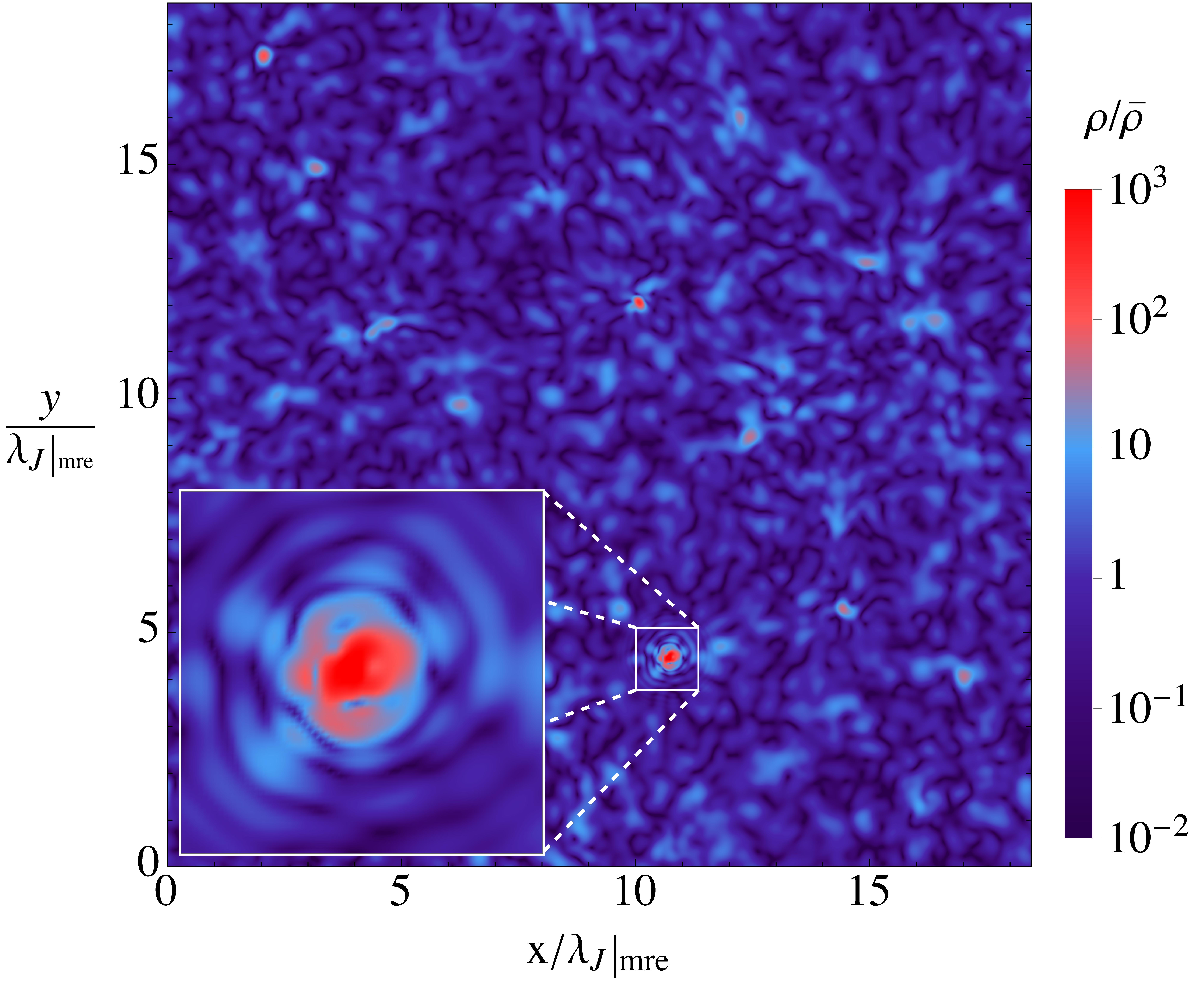
A slice of the axion density soon after MRE is plotted in Fig. 4, showing a typical star and halo.

Discussion—A key open question is the subsequent evolution of axion stars and their host halos. These may grow through accretion and mergers, potentially approaching the stability limit, or be disrupted as they are incorporated into larger structures [59, 90, 38, 84]. Analytic estimates for post-inflationary axions suggest the solitons that form around MRE are relatively robust [40], but dedicated simulations are required. Improved numerical methods, such as adaptive meshes, will be important for resolving these dynamics, as well as probing regimes with $\Delta^{2}_{a}(k_{\rm crit}|_{\rm rh})\gg 1$.

Our results have implications for direct detection searches for axions with $m_{a}\lesssim 10^{-5}\,{\,{\rm eV}}$, where EMD is best motivated, e.g., [65, 5]. If an $\mathcal{O}(1)$ fraction of axions are bound in substructure, and this survives disruption in the Solar neighbourhood, the smooth background is reduced, weakening experimental signals. The densest axion stars, which have masses around $M_{J,{\rm mre}}$ defined in Eq. (14), have radii

Collisions between the Earth and these stars are extremely rare, with the typical interval between events

assuming $20\%$ of dark matter is in objects of mass $0.1M_{J,{\rm mre}}$. More frequent transient enhancements may arise from larger-scale modes ($k<k_{\rm crit}|_{\rm rh}$) or streams from disrupted objects [88], motivating broadband searches [65]. New indirect signals may also arise [70, 89, 24, 48, 49, 63, 41, 47, 51, 98, 29, 52], e.g., photon emission during axion star–neutron star encounters [42, 11] or from caustic microlensing [36]. Although we focused on the QCD axion, similar conclusions apply to axion-like particles with EMD. It would also be interesting to explore the impact of non-gravitational couplings between the axion and modulus, as may arise in specific string compactifications.

Axion substructure also arises in the post-inflationary scenario [64, 69, 91, 43, 99]. In this case, the axion power spectrum, relative to $k_{J}|_{\rm mre}$, is similar to the case we have considered, leading to a comparable population of axion stars [58]. However, the axion masses in our scenario are much smaller than in the post-inflationary case in the absence of EMD ($m_{a}\gtrsim 10^{-4}\text{--}10^{-3}\,{\,{\rm eV}}$) [56, 57, 27, 81]. In a standard cosmological history pre-inflationary axions produce substructure only for $\theta_{0}\simeq\pi$, corresponding to large $m_{a}$ [9]. A discovery of QCD axion stars at $m_{a}\lesssim 10^{-5}\,{\,{\rm eV}}$ would therefore provide strong evidence for EMD. Conversely, a discovery of a QCD axion without substructure would constrain the early evolution of the Universe beyond current bounds from BBN.