To incorporate the effects of a non-vanishing $\gamma$, we generalize Eq. (2.8) by introducing the following helicity-dependent Ansatz for the canonically normalized mode functions $u_{k}^{\lambda}$ (which enter in the mode equation)

$$u^{\lambda}_{k}(\tau)=\frac{a(\tau)\,H}{\sqrt{2}\,k^{3/2}}\,e^{-ik\tau}\Bigg[1+ik\tau+i\,\lambda\,\sum_{n=1}^{\infty}(ik\tau_{0})^{n}\Gamma_{n}(\tau)\Bigg],$$

(2.9)

where $\lambda=\pm 1$ labels the tensor helicities, and the functions $\Gamma_{n}(\tau)$, for $n\geq 1$, encode deviations from the Bunch–Davies vacuum. The parameter $\tau_{0}$ is a reference time introduced to render the expansion dimensionless; it drops out from physical observables.

Following the strategy of [56, 57], we substitute the Ansatz (2.9) into Eq. (2.2), expand in powers of $k$, and match coefficients order by order in $k^{n}$. This procedure yields a hierarchy of coupled differential equations for the functions $\Gamma_{n}$, one for each power of $k$.

At lowest orders, one finds

	$\displaystyle\partial_{\tau}\left(\frac{\tau_{0}\,\Gamma_{1}^{\prime}(\tau)}{\tau^{2}}\right)$	$\displaystyle=\partial_{\tau}\left(\frac{\gamma^{\prime}(\tau)}{2\,\tau^{2}}\right),$		(2.10)
	$\displaystyle\partial_{\tau}\left(\frac{\tau_{0}^{2}}{\tau^{2}}\Gamma_{2}^{\prime}(\tau)\right)$	$\displaystyle=\frac{2\tau_{0}}{\tau}\partial_{\tau}\left(\frac{\Gamma_{1}(\tau)}{\tau}\right)+\frac{\tau}{2}\,\partial_{\tau}\left(\frac{1}{\tau^{2}}\gamma^{\prime}(\tau)\right),$		(2.11)

where primes denote derivatives with respect to conformal time. Higher orders follow a similar recursive structure.

The system admits a natural piecewise analysis:

1. 1.

   For $\tau<\tau_{1}$, the source vanishes ($\gamma=0$), implying $\Gamma_{n}=0$ and recovering the Bunch–Davies solution of Eq. (2.8) .

2. 2.

   For $\tau_{1}\leq\tau\leq\tau_{2}$, the source is active and the full coupled system must be solved.

3. 3.

   For $\tau>\tau_{2}$, the system returns to slow roll, and the solution is fixed by matching conditions at $\tau_{2}$.

To make analytical progress during the interval $\tau_{1}\leq\tau\leq\tau_{2}$, we assume that the source is switched on for a short time starting at $\tau_{1}$, and we impose the conditions

$$\gamma(\tau_{1})=\gamma^{\prime}(\tau_{1})=0,\qquad\beta\equiv\frac{\tau_{1}\,\gamma^{\prime\prime}(\tau_{1})}{2}\,.$$

(2.12)

This choice of these conditions – compatible with the requirements outlined after Eq. (2.6) – is crucial to carry our analytical procedure further. Taylor expanding the functions $\Gamma_{n}$ around $\tau=\tau_{1}$, and retaining the leading non-vanishing contributions, the hierarchy simplifies. It admits the following choice of derivatives as solution at $\tau=\tau_{1}$

	$\displaystyle\tau_{0}\Gamma_{1}^{(2)}(\tau_{1})$	$\displaystyle=\frac{\gamma^{\prime\prime}(\tau_{1})}{2},$		(2.13)
	$\displaystyle\tau_{0}^{2}\Gamma_{2}^{(2)}(\tau_{1})$	$\displaystyle=\frac{\tau_{1}\,\gamma^{\prime\prime}(\tau_{1})}{2},$		(2.14)
	$\displaystyle\tau_{0}^{n}\Gamma_{n}^{(n)}(\tau_{1})$	$\displaystyle=2\,\Gamma_{n-1}^{(n-1)},\qquad n>2,$		(2.15)

where superscripts indicate the order of the derivative. Based on these expressions, the solution of the system of equations leads to

	$\displaystyle\tau_{0}\Gamma_{1}(\tau)$	$\displaystyle=\frac{\beta\,(\tau-\tau_{1})^{2}}{\tau_{1}\,2!},$		(2.16)
	$\displaystyle\tau_{0}^{n}\Gamma_{n}(\tau)$	$\displaystyle=\frac{\beta\,2^{n}\,(\tau-\tau_{1})^{n}}{4\,n!},\qquad n\geq 2$		(2.17)

during the brief interval $\tau_{1}\leq\tau\leq\tau_{2}$.

Substituting back into the Ansatz (2.9), the series can be resummed in a closed form. The original tensor mode function during the transient phase reads

$\displaystyle h^{\lambda}_{k}(\tau)$

$\displaystyle=\frac{H}{\sqrt{2}\,k^{3/2}}\,e^{-ik\tau}\Bigg[1+ik\tau+\frac{i\lambda\beta}{4}\left(e^{2ik(\tau-\tau_{1})}-1-2ik(\tau-\tau_{1})\left(1-\frac{\tau-\tau_{1}}{\tau_{1}}\right)\right)\Bigg],$

(2.18)

valid for $\tau_{1}\leq\tau\leq\tau_{2}$. The parameter $\beta$ of Eq. (2.12), proportional to $\gamma^{\prime\prime}(\tau_{1})$, controls the strength of the parity-violating effects and induces helicity-dependent corrections to the mode functions. The structure of solution (2.18) depends on our Ansatz for the pump field, Eqs. (2.3) and (2.5). More general possibilities, motivated by [51], might lead to different results.

For $\tau\geq\tau_{2}$, the source switches off again and the solution of Eq. (2.2) takes the general form

$$h^{\lambda}_{k}(\tau)=\frac{H}{\sqrt{2}\,k^{3/2}}\,\left[C_{1}^{\lambda}\,e^{-ik\tau}\left(1+ik\tau\right)+C_{2}^{\lambda}\,e^{ik\tau}\left(1-ik\tau\right)\right],$$

(2.19)

where the time-independent quantities $C_{1,2}^{\lambda}$ are determined by matching $h_{k}$ and $h_{k}^{\prime}$ at $\tau=\tau_{2}$. Introducing the dimensionless, positive quantities

$$\kappa\equiv-k\tau_{1}\,,\qquad\Delta\tau\equiv-\frac{\tau_{2}-\tau_{1}}{\tau_{1}}\,,$$

(2.20)

the Israel junction conditions dictate

	$\displaystyle C_{1}^{\lambda}$	$\displaystyle=\frac{1+\beta\,\lambda\,\left[i-ie^{2i\Delta\tau\kappa}+6\Delta\tau^{2}\kappa-4i\Delta\tau^{3}\kappa^{2}+2i\Delta\tau(2+i\kappa+2\kappa^{2})\right]}{8(-1+\Delta\tau)^{2}\kappa^{2}},$
	$\displaystyle C_{2}^{\lambda}$	$\displaystyle=-\frac{e^{-2i(-1+\Delta\tau)\kappa}\,\beta\lambda\left[i+2\kappa-2\Delta\tau^{2}\kappa+4\Delta\tau(i+\kappa)+e^{2i\Delta\tau\kappa}\left(-i+2(-1+\Delta\tau)\kappa\right)\right]}{8(-1+\Delta\tau)^{2}\kappa^{2}}\,.$		(2.21)

Notice that the helicity-dependent deviation from the standard Bunch-Davies mode function is again controlled by the single parameter $\beta$, as defined in Eq. (2.12). These ingredients allow us to compute the tensor power spectrum in Fourier space at the end inflation, $\tau\to 0$, proportional to the square of the mode function $|h_{k}^{\lambda}|^{2}$ for each polarization $\lambda$:

	$\displaystyle{\cal P}_{h}^{\lambda}(k)$	$\displaystyle=$	$\displaystyle\frac{k^{3}}{4\pi^{2}}\,|h_{k}^{\lambda}|^{2}$		(2.22)
		$\displaystyle=$	$\displaystyle\frac{2H^{2}}{\pi^{2}}\,\big|C_{1}^{\lambda}+C_{2}^{\lambda}\big|^{2}\,.$		(2.23)

The total primordial tensor spectrum – related with the GW intensity – is the average of the two polarizations:

$\displaystyle{\cal P}_{h}^{T}(k)$

$\displaystyle=$

$\displaystyle\frac{1}{2}\sum_{\lambda=\pm 1}{\cal P}_{h}^{\lambda}(k)\,.$

(2.24)

At large scales, the spectrum is scale invariant, with an amplitude ${\cal P}_{h}^{T}(\kappa\ll 1)={2H^{2}}/{\pi^{2}}$. At small scales, instead, it results

$${\cal P}_{h}^{T}(\kappa\gg 1)\,=\,\frac{2H^{2}}{\pi^{2}}\,\left[1+\frac{\beta^{2}\Delta\tau^{2}\,(1+\Delta\tau)^{2}}{4(1-\Delta\tau)^{2}}\right]$$

(2.25)

Hence – in a limit of small duration of PV effects, $\Delta\tau\ll 1$ – we find an enhancement of the tensor spectrum from large towards small scales, controlled by the combination $\beta^{2}\Delta\tau^{2}$. It is important to stress the role of helicities in forming the combination (2.24). While the terms linear in $\lambda$ cancel, the terms quadratic in $\lambda^{2}$ sum up; hence, new contributions to the GW spectrum towards small scales are associated with quadratic contribution in parity-violating parameters (more on this in Section 3).

In order to investigate the specific scale dependence of the spectrum, it is convenient to compute the dimensionless ratio of the spectrum at momentum $\kappa$ versus its value at $\kappa\to 0$ [58] (the suffix $I$ indicates intensity):

$$\Pi_{I}(\kappa)\,\equiv\,\frac{{\cal P}_{h}^{T}(\kappa)}{{\cal P}_{h}^{T}(\kappa\to 0)}\,.$$

(2.26)

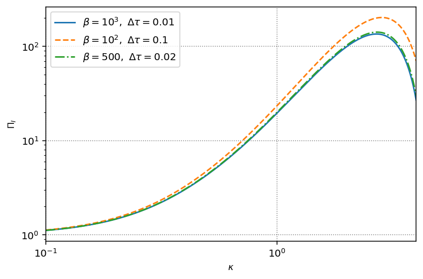
We represent the quantity $\Pi_{I}(\kappa)$ in Fig 1, left panel, for different values of the parameters $\beta$ and $\Delta\tau$. On purpose, in all cases we take $\beta$ large and $\Delta\tau$ small, keeping fixed their product. After an initial plateau for small $\kappa$ – which can allow us to satisfy present bounds on the tensor-to-scalar spectrum at CMB scales, more on this later – we notice a steady growth from large towards small scales, up to $\kappa\simeq{\cal O}(1)$ where the spectrum starts to oscillate. The resulting plots are similar for all cases. In Fig 1, right panel, we instead represent the tensor spectral index during inflation

$$n_{T}\,=\,\frac{d\ln\Pi_{I}}{d\ln\kappa}$$

(2.27)

in the growing region of the spectrum. In all cases, $n_{T}$ reaches values in the interval around $(2,2.5)$, with a limiting value at around $\sim 2.6$. Hence in our setup in which PV effects last for a short period of time, we find an universal behaviour for the growth of GW spectrum during inflation, whose slope reaches values of considerable phenomenological interest as we discuss in Section 3. Our result can be interpreted as the spin-2, parity-violating analogue of similar bounds found in other sectors. For scalar perturbations, a brief departure from slow roll leads to a maximal growth $n_{s}-1=4$ [59] (up to logarithmic corrections [60, 61]); for vector modes one finds $n_{V}\simeq 4.75$ [62, 63]; and for the longitudinal mode of a massive dark photon $n_{L}\simeq 6$ [64, 65]. Nevertheless, also in the present case, we interpret the raise of the spectrum as due to the active dynamics of the tensor decaying mode of Eq. (2.2), which becomes dominant and amplifies the amplitude of the spectrum (see e.g. [23] for a review in the context of scalar fluctuations). This specific behaviour of the decaying tensor mode is induced by the brief, but strong, phase of parity violating interactions.

For our purposes, we aim to make the duration of the parity-violating (PV) interacting phase as short as possible, $\Delta\tau\ll 1$. This ensures the validity of the Taylor expansion used in determining the mode functions. At the same time, we wish to enhance the inflationary tensor spectrum from large to small scales. This requires increasing the amplitude of PV effects, controlled by the parameter $\beta$ (see the small-scale enhancement of the spectrum, Eq. (2.25)).

A convenient and simplifying procedure, inspired by [56], is to consider the scaling limit

$$\Delta\tau\to 0\,,\qquad\qquad\beta\to\infty\,,\qquad\qquad\beta\,\Delta\tau=b_{0}=\text{fixed}\,,$$

(2.28)

where $b_{0}$ is a constant parameter. In this limit, large values of $b_{0}$ lead to a significant enhancement of the tensor spectrum, with the total growth from large to small scales scaling as $b_{0}^{2}$ (see Eq. (2.25)). Such amplification, as mentioned above, is due to the input of the would-be tensor decaying mode, which plays an active role in this set-up.

The coefficients $C_{1,2}^{\lambda}$ introduced in Eq. (2.21) simplify considerably in the limit (2.28), reducing to

	$\displaystyle C_{1}^{\lambda}$	$\displaystyle=1+\frac{i\,(1+\kappa^{2})\,\lambda\,b_{0}}{2\,\kappa^{2}}\,,$		(2.29)
	$\displaystyle C_{2}^{\lambda}$	$\displaystyle=\frac{i\,e^{2i\kappa}(i+\kappa)^{2}\,\lambda\,b_{0}}{2\,\kappa^{2}}\,.$		(2.30)

These expressions, once plugged in Eq. (2.19), make explicit the role of helicity $\lambda$ and the parity-violating parameter $b_{0}$. We find remarkable that such simple choice of mode functions catches well the effects of a transient parity-violating era during inflation.

The quantity $\Pi_{I}(\kappa)$ of Eq. (2.26), which controls the scale dependence of the tensor spectrum amplitude, is given by

$$\Pi_{I}(\kappa)=1+\frac{b_{0}^{2}(1+\kappa^{2})\left(-\kappa\cos\kappa+\sin\kappa\right)^{2}}{\kappa^{4}}\,.$$

(2.31)

Interestingly, this quantity depends only on two parameters: $b_{0}$ – which controls the amplification of the spectrum from large towards small scales – and the instant $\tau_{1}$ during inflation – which in terms of $\kappa=-k\tau_{1}$ characterizes the time at which the short PV epoch occurs.

In Fig. 2, we show $\Pi_{I}(\kappa)$ (left panel) together with its slope (right panel). This simplified expression reproduces well the qualitative features of Fig. 1. In the limit of $b_{0}$ large (which interests us) the spectrum starts and keeps almost scale invariant at large scales, i.e. within the interval $0\leq\kappa\leq\kappa_{\rm growth}$ with

$$\kappa_{\rm growth}\,=\,\frac{3}{b_{0}}\,,$$

(2.32)

where it starts growing with a profile well approximated by a power-law. (We explain the origin of Eq. (2.32) in Section 3.) Its slope in the growing region varies in a range starting at $n_{T}\simeq 2$ (recall the definition of $n_{T}$ in Eq. (2.27)) with a maximal value $n_{T}\simeq 2.6$ at around $\kappa=1$: see Fig. 2, right panel, where we zoom on the spectral tilt around the inflection point of the spectrum profile, where the rate of growth is apparent.

Phenomenological implications of this scenario, as well as a discussion of gravitational-wave Stokes parameters, are presented in what comes next.

Equation (3.1) shows that the frequency dependence of $\Omega_{\rm GW}^{(I)}$ directly traces the scale dependence of the primordial tensor spectrum. Therefore, its phenomenology might be inferred from the profiles shown in Fig. 2, expressed in terms of the dimensionless variable $\kappa$. Accordingly, the spectral tilt $n_{T}$ corresponds to the effective logarithmic slope of the GW energy density,

$$n_{T}\equiv\frac{d\ln\Omega_{\rm GW}}{d\ln f}\,,$$

(3.3)

evaluated over the relevant frequency interval.

At low frequencies, $f/f_{\star}\ll 1$, the spectrum is approximately scale invariant up to a characteristic scale $f_{\rm growth}/f_{\star}=\kappa_{\rm growth}$ (see Eq. (2.32)). Beyond this point, the spectrum grows steadily, reaching a maximum around $f/f_{\star}\sim\mathcal{O}(1)$, and subsequently develops oscillatory features for $f/f_{\star}\gtrsim 1$.

In fact, in the intermediate regime the growth can be well approximated by a power law – although the exact profile is not strictly scale-free. The effective spectral tilt varies in a range starting at $n_{T}\simeq 2$, with maximal growth occurring near an inflection point at $f/f_{\star}\simeq 1$, where it acquires a value $n_{T}=2.6$. In the limit of a short-duration PV phase, this behaviour is universal and largely insensitive to the microscopic details of the transition, as illustrated in Fig. 2. Notably, the range $n_{T}\simeq 2$ emerges naturally, and overlaps with the effective slopes obtained in PTA analyses when fitting the signal with cosmological power-law templates (see e.g. [12, 13, 14, 15, 16]).

While the effective slope provides a useful diagnostic, our scenario predicts a richer structure than a simple power law, including a transition from a nearly scale-invariant regime to a growing phase and subsequent oscillatory features. This structure, together with polarization observables we discuss in Section 3.2, offers a more robust discriminant between different physical origins of the signal.

We now combine Eqs. (2.31) and (3.1) to provide a concrete illustration of the phenomenology outlined above. (For visual reference, see Fig. 3.) In our units ($M_{\rm Pl}=1$), we obtain

$$h^{2}\,\Omega_{\rm GW}^{(I)}(f)\,=\,2.73\times 10^{-7}\,H^{2}\,\left\{1+\frac{b_{0}^{2}(f_{\star}^{2}+f^{2})\left[-f\cos\!\left({f}/{f_{\star}}\right)+f_{\star}\sin\!\left({f}/{f_{\star}}\right)\right]^{2}}{f^{4}}\right\}.$$

(3.4)

At large scales (CMB frequencies), the spectrum is approximately scale invariant. This sets a bound on the Hubble parameter $H$ during inflation. Using the approximate relation $h^{2}\Omega_{\rm GW}^{(I)}\sim 10^{-15}r$ [66], we fix the amplitude by choosing $r=10^{-3}$, which corresponds to $h^{2}\Omega_{\rm GW}^{(I)}(f\ll f_{\star})\simeq 10^{-18}$ and $H=3\times 10^{-6}$. Such values of $r$ are within reach of next-generation CMB B-mode experiments [69, 70] – hence in our setup primordial tensor modes might be detected also at CMB scales.

At larger nanohertz frequencies, current PTA observations [7, 8, 9, 10] provide evidence for a stochastic GW background with significantly larger amplitude. We can use PTA measurements to set our remaining free parameters $b_{0}$, $f_{\star}$. Adopting a power-law parameterization for the GW energy density in the PTA band, $\Omega_{\rm GW}^{(I)}(f)=A_{\star}(f/f_{\rm yr})^{n_{T}}$, Ref. [14] report the values

$$(A_{\star},n_{T})=\left(4.25^{+3.02}_{-1.92}\times 10^{-8},\;2.08^{+0.32}_{-0.30}\right)\,.$$

(3.5)

In our framework, these values can be reproduced by fixing $b_{0}$ to match the amplitude of the spectrum at small scales (which scales as $b_{0}^{2}$), and $f_{\star}$ to determine the frequency at which the spectrum begins to grow (see Fig. 3). Accordingly, we adopt $b_{0}=10^{5}$ and $f_{\star}=3.2\times 10^{-9}\,\mathrm{Hz}$ in Eq. (3.4). Importantly, the spectral slope is not a free parameter; rather, our choice ensures that the (approximate) GW power-law spectrum crosses the PTA band, with its predicted slope $n_{T}\simeq 2$. As a result, the GW spectrum remains consistent with current CMB bounds on large scales, while naturally developing the amplitude and spectral tilt compatible with PTA observations at smaller scales.²²2For this value of $f_{\star}$, Eq. (2.32) implies that the GW spectrum starts to grow only at frequencies $f_{\rm growth}\simeq 10^{-13}\,\mathrm{Hz}$, well outside the range probed by CMB polarization experiments. In Fig. 3, we compare our theoretical predictions with the sensitivity curves of current and future GW experiments in the nano-Hertz band.

While our conclusions are supported by our qualitative arguments and previous studies, it would be important to assess quantitatively and more precisely how well the GW energy density in Eq. (3.4), characterized by an approximate power-law behavior in the PTA band, fits recent PTA data. We defer this analysis to future work.

The parity-violating nature of the Chern–Simons–type couplings considered in this work generically induces a non-vanishing circular polarization. Its amplitude is controlled by a single power of the parameter $b_{0}$, see Eq. (3.7), while intensity scales as $b_{0}^{2}$. Adopting the representative value of $b_{0}$ discussed in Section 3.1, the maximal amplitude of circular polarization is expected to be significantly suppressed with respect to the intensity, e.g. by a factor $1/b_{0}\sim 10^{-5}$.

Such a suppression makes circular polarization a challenging observable for PTA measurements [72], unless one exploits parity-odd anisotropies (see e.g [73, 74] and references therein). Despite this limitation, the behaviour of $|\Pi_{V}|$, shown in Fig. 4, exhibits noteworthy features. In particular, $|\Pi_{V}|$ scales linearly with $\kappa$, and reaches the same order of magnitude as $\Pi_{I}$ precisely at the scale where $\Pi_{I}$ transitions from an approximately constant regime to a phase of growth.

We have verified that this transition occurs at the value of $\kappa$ for which the mode function $h^{R}_{k}$ vanishes when evaluated at the end of inflation, $\tau=0$. This characteristic scale coincides with $\kappa_{\rm growth}$ introduced in Eq. (2.32), and, in the large-$b_{0}$ limit, can be determined analytically using the method developed in [58] (see in particular its Section 3), by Taylor expanding the argument of $h^{R}_{k}$ in powers of $1/b_{0}$.

The linear polarization parameters $Q$ and $U$ are not scalar quantities, as they transform under rotations of the polarization angle. However, the combination $\Pi_{L}\equiv\sqrt{\Pi_{Q}^{2}+\Pi_{U}^{2}}$ is rotationally invariant, and we display it in Fig. 4. Remarkably, in the present setup this quantity can become large, with both its amplitude and scale dependence closely tracking those of the intensity at small scales. From Eqs. (3.7), this behavior originates from the fact that $\Pi_{I}$ and $\Pi_{Q}$ scale quadratically with the parameter $b_{0}$, while $\Pi_{U}$ is only linear in $b_{0}$.

As a result, in the PTA band the linear polarization fraction satisfies

$$\Pi_{L}\simeq\Pi_{I}\,,$$

(3.8)

up to small corrections controlled by $\Pi_{V}/\Pi_{I}$. This implies that the stochastic background is nearly maximally linearly polarized at the scales of interest. Such a large linear polarization signal would constitute a striking observational signature of our scenario, especially in view of the fact that typical astrophysical sources are expected to generate only a small degree of linear polarization, at the level of a few percent of the total intensity [75]. If detectable—for instance, with techniques such as those proposed in [76, 77]—this feature would provide a strong indication of a cosmological origin of the signal. Hence dedicated forecasts to assess the sensitivity of forthcoming PTA experiments to such observables would therefore be desirable. And besides experimental consequences, such a large linear polarization has interesting theoretical ramifications too, as we are going to discuss.

References

- [1] A. A. Starobinsky, “A New Type of Isotropic Cosmological Models Without Singularity,” Phys. Lett. B 91 (1980) 99–102.
- [2] A. H. Guth, “The Inflationary Universe: A Possible Solution to the Horizon and Flatness Problems,” Phys. Rev. D 23 (1981) 347–356.
- [3] A. D. Linde, “A New Inflationary Universe Scenario: A Possible Solution of the Horizon, Flatness, Homogeneity, Isotropy and Primordial Monopole Problems,” Phys. Lett. B 108 (1982) 389–393.
- [4] A. A. Starobinsky, “Spectrum of relict gravitational radiation and the early state of the universe,” JETP Lett. 30 (1979) 682–685.
- [5] M. Kamionkowski and E. D. Kovetz, “The Quest for B Modes from Inflationary Gravitational Waves,” Ann. Rev. Astron. Astrophys. 54 (2016) 227–269, arXiv:1510.06042 [astro-ph.CO].
- [6] N. Bartolo et al., “Science with the space-based interferometer LISA. IV: Probing inflation with gravitational waves,” JCAP 12 (2016) 026, arXiv:1610.06481 [astro-ph.CO].
- [7] NANOGrav Collaboration, G. Agazie et al., “The NANOGrav 15 yr Data Set: Evidence for a Gravitational-wave Background,” Astrophys. J. Lett. 951 no. 1, (2023) L8, arXiv:2306.16213 [astro-ph.HE].
- [8] D. J. Reardon et al., “Search for an Isotropic Gravitational-wave Background with the Parkes Pulsar Timing Array,” Astrophys. J. Lett. 951 no. 1, (2023) L6, arXiv:2306.16215 [astro-ph.HE].
- [9] H. Xu et al., “Searching for the Nano-Hertz Stochastic Gravitational Wave Background with the Chinese Pulsar Timing Array Data Release I,” Res. Astron. Astrophys. 23 no. 7, (2023) 075024, arXiv:2306.16216 [astro-ph.HE].
- [10] EPTA, InPTA: Collaboration, J. Antoniadis et al., “The second data release from the European Pulsar Timing Array - III. Search for gravitational wave signals,” Astron. Astrophys. 678 (2023) A50, arXiv:2306.16214 [astro-ph.HE].
- [11] R. Jackiw and S. Y. Pi, “Chern-Simons modification of general relativity,” Phys. Rev. D 68 (2003) 104012, arXiv:gr-qc/0308071.
- [12] NANOGrav Collaboration, A. Afzal et al., “The NANOGrav 15 yr Data Set: Search for Signals from New Physics,” Astrophys. J. Lett. 951 no. 1, (2023) L11, arXiv:2306.16219 [astro-ph.HE]. [Erratum: Astrophys.J.Lett. 971, L27 (2024), Erratum: Astrophys.J. 971, L27 (2024)].
- [13] EPTA, InPTA Collaboration, J. Antoniadis et al., “The second data release from the European Pulsar Timing Array - IV. Implications for massive black holes, dark matter, and the early Universe,” Astron. Astrophys. 685 (2024) A94, arXiv:2306.16227 [astro-ph.CO].
- [14] D. G. Figueroa, M. Pieroni, A. Ricciardone, and P. Simakachorn, “Cosmological Background Interpretation of Pulsar Timing Array Data,” Phys. Rev. Lett. 132 no. 17, (2024) 171002, arXiv:2307.02399 [astro-ph.CO].
- [15] S. Vagnozzi, “Inflationary interpretation of the stochastic gravitational wave background signal detected by pulsar timing array experiments,” JHEAp 39 (2023) 81–98, arXiv:2306.16912 [astro-ph.CO].
- [16] J. Ellis, M. Fairbairn, G. Franciolini, G. Hütsi, A. Iovino, M. Lewicki, M. Raidal, J. Urrutia, V. Vaskonen, and H. Veermäe, “What is the source of the PTA GW signal?,” Phys. Rev. D 109 no. 2, (2024) 023522, arXiv:2308.08546 [astro-ph.CO].
- [17] A. Sesana and D. G. Figueroa, “Nanohertz Gravitational Waves,” arXiv:2512.18822 [astro-ph.CO].
- [18] C. Fu, J. Liu, X.-Y. Yang, W.-W. Yu, and Y. Zhang, “Explaining pulsar timing array observations with primordial gravitational waves in parity-violating gravity,” Phys. Rev. D 109 no. 6, (2024) 063526, arXiv:2308.15329 [astro-ph.CO].
- [19] X. Niu and M. H. Rahat, “NANOGrav signal from axion inflation,” Phys. Rev. D 108 (2023) no.11, 11 doi:10.1103/PhysRevD.108.115023 [arXiv:2307.01192 [hep-ph]].
- [20] C. Caprini and D. G. Figueroa, “Cosmological Backgrounds of Gravitational Waves,” Class. Quant. Grav. 35 no. 16, (2018) 163001, arXiv:1801.04268 [astro-ph.CO].
- [21] LISA Cosmology Working Group Collaboration, P. Auclair et al., “Cosmology with the Laser Interferometer Space Antenna,” Living Rev. Rel. 26 no. 1, (2023) 5, arXiv:2204.05434 [astro-ph.CO].
- [22] G. Domènech, “Scalar Induced Gravitational Waves Review,” Universe 7 no. 11, (2021) 398, arXiv:2109.01398 [gr-qc].
- [23] O. Özsoy and G. Tasinato, “Inflation and Primordial Black Holes,” Universe 9 no. 5, (2023) 203, arXiv:2301.03600 [astro-ph.CO].
- [24] LISA Cosmology Working Group Collaboration, J. E. Gammal et al., “Reconstructing primordial curvature perturbations via scalar-induced gravitational waves with LISA,” JCAP 05 (2025) 062, arXiv:2501.11320 [astro-ph.CO].
- [25] B. Carr, A. J. Iovino, G. Perna, V. Vaskonen, and H. Veermäe, “Primordial black holes: constraints, potential evidence and prospects,” arXiv:2601.06024 [astro-ph.CO].
- [26] L. Liu, Z.-C. Chen, and Q.-G. Huang, “Probing the equation of state of the early Universe with pulsar timing arrays,” JCAP 11 (2023) 071, arXiv:2307.14911 [astro-ph.CO].
- [27] G. Domènech, S. Pi, A. Wang, and J. Wang, “Induced gravitational wave interpretation of PTA data: a complete study for general equation of state,” JCAP 08 (2024) 054, arXiv:2402.18965 [astro-ph.CO].
- [28] K. Harigaya, K. Inomata, and T. Terada, “Induced gravitational waves with kination era for recent pulsar timing array signals,” Phys. Rev. D 108 no. 12, (2023) 123538, arXiv:2309.00228 [astro-ph.CO].
- [29] S. Balaji, G. Domènech, and G. Franciolini, “Scalar-induced gravitational wave interpretation of PTA data: the role of scalar fluctuation propagation speed,” JCAP 10 (2023) 041, arXiv:2307.08552 [gr-qc].
- [30] G. Franciolini, A. Iovino, Junior., V. Vaskonen, and H. Veermae, “Recent Gravitational Wave Observation by Pulsar Timing Arrays and Primordial Black Holes: The Importance of Non-Gaussianities,” Phys. Rev. Lett. 131 no. 20, (2023) 201401, arXiv:2306.17149 [astro-ph.CO].
- [31] L. Liu, Z.-C. Chen, and Q.-G. Huang, “Implications for the non-Gaussianity of curvature perturbation from pulsar timing arrays,” Phys. Rev. D 109 no. 6, (2024) L061301, arXiv:2307.01102 [astro-ph.CO].
- [32] L. Liu, Y. Wu, and Z.-C. Chen, “Simultaneously probing the sound speed and equation of state of the early Universe with pulsar timing arrays,” JCAP 04 (2024) 011, arXiv:2310.16500 [astro-ph.CO].
- [33] S. Endlich, A. Nicolis, and J. Wang, “Solid Inflation,” JCAP 10 (2013) 011, arXiv:1210.0569 [hep-th].
- [34] D. Cannone, G. Tasinato, and D. Wands, “Generalised tensor fluctuations and inflation,” JCAP 01 (2015) 029, arXiv:1409.6568 [astro-ph.CO].
- [35] N. Bartolo, D. Cannone, A. Ricciardone, and G. Tasinato, “Distinctive signatures of space-time diffeomorphism breaking in EFT of inflation,” JCAP 03 (2016) 044, arXiv:1511.07414 [astro-ph.CO].
- [36] M. Mylova, O. Özsoy, S. Parameswaran, G. Tasinato, and I. Zavala, “A new mechanism to enhance primordial tensor fluctuations in single field inflation,” JCAP 12 (2018) 024, arXiv:1808.10475 [gr-qc].
- [37] O. Ozsoy, M. Mylova, S. Parameswaran, C. Powell, G. Tasinato, and I. Zavala, “Squeezed tensor non-Gaussianity in non-attractor inflation,” JCAP 09 (2019) 036, arXiv:1902.04976 [hep-th].
- [38] L. Frosina and A. Urbano, “Inflationary interpretation of the nHz gravitational-wave background,” Phys. Rev. D 108 no. 10, (2023) 103544, arXiv:2308.06915 [astro-ph.CO].
- [39] G. Ferrante, G. Franciolini, A. Iovino, Junior., and A. Urbano, “Primordial black holes in the curvaton model: possible connections to pulsar timing arrays and dark matter,” JCAP 06 (2023) 057, arXiv:2305.13382 [astro-ph.CO].
- [40] M. A. Gorji, M. Sasaki, and T. Suyama, “Extra-tensor-induced origin for the PTA signal: No primordial black hole production,” Phys. Lett. B 846 (2023) 138214, arXiv:2307.13109 [astro-ph.CO].
- [41] A. Lue, L.-M. Wang, and M. Kamionkowski, “Cosmological signature of new parity violating interactions,” Phys. Rev. Lett. 83 (1999) 1506–1509, arXiv:astro-ph/9812088.
- [42] S. H.-S. Alexander, M. E. Peskin, and M. M. Sheikh-Jabbari, “Leptogenesis from gravity waves in models of inflation,” Phys. Rev. Lett. 96 (2006) 081301, arXiv:hep-th/0403069.
- [43] M. Satoh, S. Kanno, and J. Soda, “Circular Polarization of Primordial Gravitational Waves in String-inspired Inflationary Cosmology,” Phys. Rev. D 77 (2008) 023526, arXiv:0706.3585 [astro-ph].
- [44] M. M. Anber and L. Sorbo, “Naturally inflating on steep potentials through electromagnetic dissipation,” Phys. Rev. D 81 (2010) 043534, arXiv:0908.4089 [hep-th].
- [45] C. R. Contaldi, J. Magueijo, and L. Smolin, “Anomalous CMB polarization and gravitational chirality,” Phys. Rev. Lett. 101 (2008) 141101, arXiv:0806.3082 [astro-ph].
- [46] S. Alexander and N. Yunes, “Chern-Simons Modified General Relativity,” Phys. Rept. 480 (2009) 1–55, arXiv:0907.2562 [hep-th].
- [47] T. D. Lee and C.-N. Yang, “Question of Parity Conservation in Weak Interactions,” Phys. Rev. 104 (1956) 254–258.
- [48] C. S. Wu, E. Ambler, R. W. Hayward, D. D. Hoppes, and R. P. Hudson, “Experimental Test of Parity Conservation in Decay,” Phys. Rev. 105 (1957) 1413–1414.
- [49] D. Cannone, J.-O. Gong, and G. Tasinato, “Breaking discrete symmetries in the effective field theory of inflation,” JCAP 08 (2015) 003, arXiv:1505.05773 [hep-th].
- [50] P. Creminelli, J. Gleyzes, J. Noreña, and F. Vernizzi, “Resilience of the standard predictions for primordial tensor modes,” Phys. Rev. Lett. 113 no. 23, (2014) 231301, arXiv:1407.8439 [astro-ph.CO].
- [51] M. Crisostomi, K. Noui, C. Charmousis, and D. Langlois, “Beyond Lovelock gravity: Higher derivative metric theories,” Phys. Rev. D 97 no. 4, (2018) 044034, arXiv:1710.04531 [hep-th].
- [52] X. Gao and X.-Y. Hong, “Propagation of gravitational waves in a cosmological background,” Phys. Rev. D 101 no. 6, (2020) 064057, arXiv:1906.07131 [gr-qc].
- [53] T. Zhu, W. Zhao, and A. Wang, “Gravitational wave constraints on spatial covariant gravities,” Phys. Rev. D 107 no. 4, (2023) 044051, arXiv:2211.04711 [gr-qc].
- [54] P. H. C. Lau, K. Nishii, and T. Noumi, “Gravitational EFT for dissipative open systems,” JHEP 02 (2025) 155, arXiv:2412.21136 [hep-th].
- [55] S. A. Salcedo, T. Colas, L. Dufner, and E. Pajer, “An open system approach to gravity,” JHEP 02 (2026) 241, arXiv:2507.03103 [hep-th].
- [56] G. Tasinato, “Large || approach to single field inflation,” Phys. Rev. D 108 no. 4, (2023) 043526, arXiv:2305.11568 [hep-th].
- [57] G. Tasinato, “Non-Gaussianities and the large || approach to inflation,” Phys. Rev. D 109 no. 6, (2024) 063510, arXiv:2312.03498 [hep-th].
- [58] G. Tasinato, “An analytic approach to non-slow-roll inflation,” Phys. Rev. D 103 no. 2, (2021) 023535, arXiv:2012.02518 [hep-th].
- [59] C. T. Byrnes, P. S. Cole, and S. P. Patil, “Steepest growth of the power spectrum and primordial black holes,” JCAP 06 (2019) 028, arXiv:1811.11158 [astro-ph.CO].
- [60] P. Carrilho, K. A. Malik, and D. J. Mulryne, “Dissecting the growth of the power spectrum for primordial black holes,” Phys. Rev. D 100 no. 10, (2019) 103529, arXiv:1907.05237 [astro-ph.CO].
- [61] O. Özsoy and G. Tasinato, “On the slope of the curvature power spectrum in non-attractor inflation,” JCAP 04 (2020) 048, arXiv:1912.01061 [astro-ph.CO].
- [62] B. Atkins, D. Chowdhury, A. Marriott-Best, and G. Tasinato, “Inflationary magnetogenesis beyond slow-roll and its induced gravitational waves,” Phys. Rev. D 112 no. 6, (2025) 063534, arXiv:2507.01772 [astro-ph.CO].
- [63] H. V. Ragavendra, G. Tasinato, and L. Sriramkumar, “Chiral gravitational waves from multi-phase magnetogenesis,” arXiv:2602.16575 [astro-ph.CO].
- [64] A. Marriott-Best, M. Peloso, and G. Tasinato, “New gravitational wave probe of vector dark matter,” Phys. Rev. D 111 no. 10, (2025) 103511, arXiv:2502.13116 [astro-ph.CO].
- [65] M. La Rosa and G. Tasinato, “Ultralight dark matter from non-slow-roll inflation,” Phys. Rev. D 112 no. 12, (2025) 123542, arXiv:2508.16455 [astro-ph.CO].
- [66] M. Maggiore, Gravitational Waves. Vol. 2: Astrophysics and Cosmology. Oxford University Press, 3, 2018.
- [67] BICEP2, Keck Array Collaboration, P. A. R. Ade et al., “BICEP2 / Keck Array x: Constraints on Primordial Gravitational Waves using Planck, WMAP, and New BICEP2/Keck Observations through the 2015 Season,” Phys. Rev. Lett. 121 (2018) 221301, arXiv:1810.05216 [astro-ph.CO].
- [68] K. Schmitz, “New Sensitivity Curves for Gravitational-Wave Signals from Cosmological Phase Transitions,” JHEP 01 (2021) 097, arXiv:2002.04615 [hep-ph].
- [69] LiteBIRD Collaboration, E. Allys et al., “Probing Cosmic Inflation with the LiteBIRD Cosmic Microwave Background Polarization Survey,” PTEP 2023 no. 4, (2023) 042F01, arXiv:2202.02773 [astro-ph.IM].
- [70] CMB-S4 Collaboration, K. Abazajian et al., “Snowmass 2021 CMB-S4 White Paper,” arXiv:2203.08024 [astro-ph.CO].
- [71] T. L. Smith and R. Caldwell, “Sensitivity to a Frequency-Dependent Circular Polarization in an Isotropic Stochastic Gravitational Wave Background,” Phys. Rev. D 95 no. 4, (2017) 044036, arXiv:1609.05901 [gr-qc].
- [72] R. Kato and J. Soda, “Probing circular polarization in stochastic gravitational wave background with pulsar timing arrays,” Phys. Rev. D 93 no. 6, (2016) 062003, arXiv:1512.09139 [gr-qc].
- [73] G. Tasinato, “Kinematic anisotropies and pulsar timing arrays,” Phys. Rev. D 108 no. 10, (2023) 103521, arXiv:2309.00403 [gr-qc].
- [74] N. M. J. Cruz, A. Malhotra, G. Tasinato, and I. Zavala, “Measuring the circular polarization of gravitational waves with pulsar timing arrays,” Phys. Rev. D 110 no. 10, (2024) 103505, arXiv:2406.04957 [astro-ph.CO].
- [75] G. Sato-Polito and M. Kamionkowski, “Exploring the spectrum of stochastic gravitational-wave anisotropies with pulsar timing arrays,” Phys. Rev. D 109 no. 12, (2024) 123544, arXiv:2305.05690 [astro-ph.CO].
- [76] Y.-K. Chu, G.-C. Liu, and K.-W. Ng, “Observation of a polarized stochastic gravitational-wave background in pulsar-timing-array experiments,” Phys. Rev. D 104 no. 12, (2021) 124018, arXiv:2107.00536 [gr-qc].
- [77] N. Anil Kumar, M. Çalışkan, G. Sato-Polito, M. Kamionkowski, and L. Ji, “Linear polarization of the stochastic gravitational-wave background with pulsar timing arrays,” Phys. Rev. D 110 no. 4, (2024) 043501, arXiv:2312.03056 [astro-ph.CO].
- [78] L. P. Grishchuk and Y. V. Sidorov, “On the Quantum State of Relic Gravitons,” Class. Quant. Grav. 6 (1989) L161–L165.
- [79] L. P. Grishchuk and Y. V. Sidorov, “Squeezed quantum states of relic gravitons and primordial density fluctuations,” Phys. Rev. D 42 (1990) 3413–3421.
- [80] M. Ciprini, M. L. Marcelli, and G. Tasinato, “Probing Gravitational-Wave Four-Point Correlators,” arXiv:2603.15514 [astro-ph.CO].