跳到论文正文
W Papers独立论文阅读器 arXiv:2604.26449 论文正文 计算阅读时间 · 0%
引用这篇论文根据当前论文元数据生成,正式投稿前建议核对。


License: CC BY-NC-ND 4.0
arXiv:2604.26449v2 [math.NA] 04 Aug 2026

Multiscale Modeling for Time-harmonic Maxwell equations with impedance boundary conditions in highly heterogeneous media

Xiang Zhong Department of Mathematics, The Chinese University of Hong Kong, Shatin, Hong Kong SAR, China. Eric T. Chung Department of Mathematics, The Chinese University of Hong Kong, Shatin, Hong Kong SAR, China. Xingguang Jin Corresponding author. (Email address: xgjin@math.cuhk.edu.hk) Department of Mathematics, The Chinese University of Hong Kong, Shatin, Hong Kong SAR, China.
Abstract

Modeling time-harmonic Maxwell problems in heterogeneous media presents significant mathematical and computational challenges. Due to the inherent non-elliptic structure and non-coercive nature of Maxwell equations, conventional methods face severe numerical instabilities, particularly in high-contrast media and at high wave numbers. These challenges often lead to ill-conditioned discrete systems and prohibitively high computational costs, limiting their practical applicability. To overcome these challenges, we introduce an efficient multiscale framework for time-harmonic Maxwell equations with impedance boundary conditions in high-contrast media. A major novelty of this study lies in circumventing the need for an explicit divergence-free constraint on multiscale basis functions. To achieve this, an auxiliary space is constructed via local spectral problems incorporating a mass term and a Silver-Müller-type boundary penalty. This novel design guarantees the coercivity of the corresponding bilinear form and automatically excludes the kernel of the curl operator from the leading eigenspaces. Building upon the auxiliary space, we then construct the multiscale space by using a distinct bilinear form. By exploiting a resolution condition and establishing key norm relationships, we rigorously prove the coercivity of this modified bilinear form—a crucial property that underpins the whole analysis. Theoretical analysis shows that, with appropriate oversampling, the method achieves O​(H)O(H) convergence independent of the local contrast and the approximation error increases with the wave number kk. Extensive numerical experiments are reported to validate the effectiveness of the proposed approach.

Keywords: Maxwell problem, high contrast coefficients, multiscale method, resolution condition

1 Introduction

The study of time-harmonic Maxwell’s equations is fundamental in modern electromagnetics, especially with the rapid advancement of electromagnetic metamaterials. These are artificially engineered structures that manipulate waves in ways not possible with natural materials [36, 29]. By arranging subwavelength meta-atoms, metamaterials can achieve unusual properties such as negative refraction, cloaking, and superlensing [24, 34, 23, 22]. Photonic crystals are key examples that utilize periodic dielectric variations to engineer photonic band structures via Bragg scattering. Such lattices can either suppress wave propagation through photonic band gaps or facilitate unique phenomena like slow light and self-collimation [27, 33].

Despite substantial mathematical progress in understanding complex electromagnetic phenomena [28], the simulation of wave propagation in highly heterogeneous media remains a formidable challenge. Traditional numerical schemes for the time-harmonic Maxwell’s equations, such as standard finite element or finite difference methods, often become computationally prohibitive in the presence of microscale heterogeneities. Resolving these fine-scale features necessitates extremely refined meshes, leading to excessive computational costs and ill-conditioned algebraic systems [16]. Beyond the multiscale nature of the problem, the high-wavenumber regime remains particularly challenging despite various numerical demonstrations. Moreover, the emergence of unconventional coefficients and the non-coercive nature inherent in metamaterial modeling frequently undermine traditional numerical analysis frameworks. While classical homogenization theory offers a path toward effective macroscopic models, its applicability is often limited by restrictive structural assumptions [1].

To address these difficulties, multiscale methods have emerged as a powerful paradigm, designed to embed fine-scale information directly into coarse-scale basis functions. A diverse array of such techniques has been developed, including multiscale finite element methods (MsFEMs) [19, 11], general multiscale finite element methods (GMsFEM) [5], localized orthogonal decomposition (LOD) [26], variational multiscale methods [20], numerical upscaling [32], heterogeneous multiscale methods (HMM) [9, 10, 12], and numerical homogenization [37]. Specifically, in the context of electromagnetic waves, significant advancements have been made through multiscale asymptotic methods and HMMs to construct efficient coarse-scale models [2, 8, 14], with extensions addressing time-domain analysis [17], high-contrast materials [35], and LOD-based computational homogenization [15]. Despite their success, the performance of these approaches generally hinges on the explicit construction of stable correctors or specific structural properties such as periodicity. In contrast, the Constrained Energy Minimization Generalized Multiscale Finite Element Method (CEM-GMsFEM) [4, 3, 40, 39, 7] provides a robust alternative by constructing multiscale basis functions via energy minimization subject to local constraints on the coarse grid. This framework naturally accommodates high-contrast coefficients without the need for specific quasi-interpolation stability, allows for systematic control over the energy-norm error, and offers the flexibility to incorporate local spectral information. Consequently, CEM-GMsFEM delivers a highly efficient computational methodology for challenging electromagnetic simulations involving complex geometries and extreme heterogeneities.

In this work, we consider the time-harmonic Maxwell equations at a fixed angular frequency ω>0\omega>0 in free space (i.e. the relative permittivity εr≡1\varepsilon_{r}\equiv 1) containing highly heterogeneous magnetic material described by the relative permeability μr​(𝐱)∈L∞​(Ω)\mu_{r}(\mathbf{x})\in L^{\infty}(\Omega) that may vary over several orders of magnitude. More precisely, for μr​(𝐱)\mu_{r}(\mathbf{x}), we suppose there exist positive constants 0<μ\operatorfont​m​i​n≤μ\operatorfont​m​a​x0<\mu_{{\operatorfont min}}\leq\mu_{{\operatorfont max}} such that for a.e. 𝐱∈Ω\mathbf{x}\in\Omega, μ\operatorfont​m​i​n≤μr​(𝐱)≤μ\operatorfont​m​a​x\mu_{{\operatorfont min}}\leq\mu_{r}(\mathbf{x})\leq\mu_{{\operatorfont max}}. We assume the system is non-conductive (i.e. the conductivity σ≡0\sigma\equiv 0). Let Ω⊂ℝ3\Omega\subset\mathbb{R}^{3} be a bounded connected Lipschitz domain. The problem is to find the electric field 𝒖∈ℂ3\bm{u}\in\mathbb{C}^{3} corresponding to a given current density 𝐟\mathbf{f} such that the following system holds:

curl⁡(μr−1​curl⁡𝐮)−k2​𝐮\displaystyle\operatorname{curl}\left(\mu_{r}^{-1}\operatorname{curl}\mathbf{u}\right)-k^{2}\mathbf{u} =𝐟\displaystyle=\mathbf{f} in ​Ω,\displaystyle\text{in }\Omega, (1a)
μr−1​curl⁡𝐮×𝐧−i​k​𝐮T\displaystyle\mu_{r}^{-1}\operatorname{curl}\mathbf{u}\times\mathbf{n}-ik\mathbf{u}_{T} =𝐠\displaystyle=\mathbf{g} on ​∂Ω,\displaystyle\text{on }\partial\Omega, (1b)

where k=ω/c0=ω​ε0​μ0>0k=\omega/c_{0}=\omega\sqrt{\varepsilon_{0}\mu_{0}}>0 is the (fixed) free-space wavenumber. Here ε0\varepsilon_{0} and μ0\mu_{0} denote the vacuum permittivity and permeability, respectively, and c0=1/ε0​μ0c_{0}=1/\sqrt{\varepsilon_{0}\mu_{0}} the speed of light in vacuum. 𝐠\mathbf{g} is a given tangential vector field on the boundary ∂Ω\partial\Omega. 𝐧\mathbf{n} is the unit outward normal vector on ∂Ω\partial\Omega. 𝐰T=(𝐧×𝐰)×𝐧=𝐰−(𝐰⋅𝐧)​𝐧\mathbf{w}_{T}=(\mathbf{n}\times\mathbf{w})\times\mathbf{n}=\mathbf{w}-(\mathbf{w}\cdot\mathbf{n})\mathbf{n} denotes the tangential component trace. The boundary condition (1b) is the first-order Silver–Müller absorbing condition, which is just an impedance boundary condition with the impedance parameter λ=1\lambda=1 (also with μr=1\mu_{r}=1 on ∂Ω\partial\Omega and εr=μr=1\varepsilon_{r}=\mu_{r}=1 in a neighborhood of ∂Ω\partial\Omega, see [28]). The presence of the imaginary unit ii introduces a phase shift, which allows the boundary to partially transmit and reflect incoming waves. This key feature enables the simulation of wave radiation into open space, making it possible to model unbounded wave scattering and radiation problems within a finite computational domain Ω\Omega. We restrict ourselves to the case εr≡1\varepsilon_{r}\equiv 1 primarily to isolate the effect of high-contrast permeability. More precisely, we focus on heterogeneous media with high-contrast permeability μr\mu_{r} at a fixed wavenumber kk, rather than on the additional complications caused by simultaneous high contrast in both constitutive parameters or by the high-frequency asymptotic regime. Similar one-parameter settings are commonly used to highlight the dominant physical mechanism, such as dielectric-dominant or magnetic-dominant responses [30, 18]. Physically, this model describes electromagnetic wave scattering and propagation in air or vacuum, perturbed by the presence of strongly heterogeneous, purely magnetic inclusions or metamaterials. Typical applications include the modeling of ferrites, magnetic cloaks, μ\mu-near-zero structures, magnetic photonic crystals, and magnetic radar-absorbing materials.

We propose an efficient multiscale framework for time-harmonic Maxwell equations with impedance boundary conditions in heterogeneous media. The method constructs multiscale basis functions tailored for highly heterogeneous media in two stages. In the first stage, an auxiliary multiscale space is built for each coarse element by solving local spectral problems. Notably, no divergence-free constraint—either weak or strong—is imposed during this construction. This is because the local spectral problem incorporates a mass term and a Silver–Müller-type boundary penalty term, which together ensure the coercivity of the associated bilinear form. As a result, the kernel of the curl operator is automatically excluded from the dominant eigenspaces, eliminating the need for explicit enforcement of the divergence-free condition on the local auxiliary multiscale basis functions. The design of the local spectral problems proposed in this study represents a novel departure from existing approaches, a feature that has not been fully addressed in prior literature [2, 8, 14, 17, 35, 15]. In the second stage, the auxiliary multiscale space is used to construct the final multiscale space. Unlike traditional construction strategies [4, 6], the bilinear form employed in this stage differs from the coercive form used in the first stage. Therefore, establishing the coercivity of a more complex bilinear form becomes essential for the subsequent theoretical analysis. Leveraging a suitable resolution condition and relationships between various norms, we establish the desired coercivity. By appropriately selecting the number of graph oversampling layers, we achieve an O​(H)O(H) convergence that is independent of the local contrast. Meanwhile, the approximation error increases with the wave number.

We provide more detailed comparisons with several existing multiscale methods for Maxwell equations [8, 14, 15, 5, 37]. HMM-based methods [8, 14] mainly focus on periodic or scale-separated media, while the LOD framework [15] relies on the construction of stable correctors and may require restrictive resolution conditions in strongly heterogeneous settings. The adaptive GMsFEM of Chung and Li [5] was developed for coercive H​(curl)H(\mathrm{curl})-elliptic problems and therefore differs fundamentally from the indefinite Maxwell setting considered here. More recently, [37] proposed a numerical homogenization approach for indefinite time-harmonic Maxwell equations based on an edge multiscale approach. For these Maxwell multiscale methods, the treatment of the kernel of the curl operator is often a central issue and may involve divergence-free constraints, auxiliary saddle-point formulations, or additional projection procedures. In contrast, the proposed local spectral problem in our work incorporates a positive mass term and a Silver–Müller-type boundary penalty, which automatically suppresses curl-kernel modes in the auxiliary space construction. From an implementation viewpoint, the proposed spectral problem avoids imposing explicit divergence-free constraints in both the local spectral problems and the multiscale basis construction, thereby simplifying the local basis generation procedure. Moreover, compared with HMM [8, 14] and LOD [15] approaches, our work is particularly attractive for high-contrast heterogeneous media. This allows the method to accommodate more complicated heterogeneous structures encountered in practical applications. The auxiliary space is obtained through local eigenvalue problems that directly identify the dominant multiscale features associated with the coefficient heterogeneity. This construction leads to a contrast-independent O​(H)O(H) convergence theory and provides a systematic mechanism for selecting multiscale basis functions that remain robust in high-contrast media.

We emphasize that the present work goes beyond a direct extension of existing CEM-GMsFEM techniques [4, 3, 40].The main challenge is to construct a Maxwell-compatible multiscale framework capable of handling the non-coercive and non-Hermitian structure of the time-harmonic Maxwell system. In particular, we introduce a new local spectral problem that avoids explicit divergence-free constraints, develop a Petrov–Galerkin multiscale formulation with distinct trial and test spaces, and establish new stability and localization property that are required for the indefinite and non-Hermitian Maxwell setting – results that do not follow directly from the existing CEM-GMsFEM theory. These developments lead to a rigorous, contrast-independent O​(H)O(H) convergence for heterogeneous Maxwell problems with impedance boundary conditions.

We also point out that the proposed multiscale framework is not limited to εr=1\varepsilon_{r}=1. Our analysis can be adapted to the case where εr​(𝐱)\varepsilon_{r}(\mathbf{x}) is also heterogeneous. Indeed, the extension mainly requires replacing the standard mass term by the weighted term involving εr\varepsilon_{r}, while the multiscale basis construction, localization analysis, and stability arguments can be adapted with minor modifications. If εr​(𝐱)\varepsilon_{r}(\mathbf{x}) also exhibits high contrast, the corresponding resolution condition may become more restrictive due to the additional dependence on the contrast of εr\varepsilon_{r}.

This paper is organized as follows. In Section 2, we introduce some notation and definitions. The construction of the multiscale basis functions in the proposed method is described in Section 3. All theoretical results and error analyses for the proposed method are presented in Section 4. To assess the performance of the proposed approach, numerical experiments on three representative models are reported in Section 5. Finally, conclusions and perspectives for future work are given in Section 6.

2 Preliminaries

In this paper, vector-valued functions are denoted by boldface letters and, unless specified, are complex-valued. Throughout this paper, we use standard notation: For a domain D∈ΩD\in\Omega, L2​(D)L^{2}(D) denotes the usual complex Lebesgue space with norm ∥⋅∥Lp​(D)\|\cdot\|_{L^{p}(D)}. If D=ΩD=\Omega, then we may drop the subscript DD. Vector space is represented in bold black italics, for instance, 𝑳2​(D)≔[L2​(D)]3\bm{L}^{2}(D)\coloneqq[L^{2}(D)]^{3}. The dot denotes the standard scalar product. We adopt the convention that the complex scalar product is conjugate-linear in the second argument, with 𝐯¯\overline{\mathbf{v}} denoting the complex conjugate of 𝐯\mathbf{v}. The vector-valued Hilbert space 𝑯​(curl,D)\bm{H}(\mathrm{curl},D) is defined as 𝑯​(curl,D)≔{𝐮∈𝑳2​(D):curl​𝐮∈𝑳2​(D)}\bm{H}(\mathrm{curl},D)\coloneqq\{\mathbf{u}\in\bm{L}^{2}(D)\colon\mathrm{curl}\,\mathbf{u}\in\bm{L}^{2}(D)\}, equipped with its standard graph norm scalar product (⋅,⋅)H​(curl,D)(\cdot,\cdot)_{H(\mathrm{curl},D)}.

Define the following vector spaces

𝑳t2​(∂Ω)\displaystyle\bm{L}_{t}^{2}(\partial\Omega) ≔{𝐯∈𝑳2​(∂Ω):𝐯⋅𝐧=0},\displaystyle\coloneqq\left\{\mathbf{v}\in\bm{L}^{2}(\partial\Omega)\colon\mathbf{v}\cdot\mathbf{n}=0\right\},
𝑽\displaystyle\bm{V} ≔𝑯imp​(curl;Ω)={𝐯∈𝑯​(curl,Ω):𝐯T∈𝑳2​(∂Ω)}\displaystyle\coloneqq\bm{H}_{\mathrm{imp}}(\operatorname{curl};\Omega)=\left\{\mathbf{v}\in\bm{H}(\operatorname{curl},\Omega)\colon\mathbf{v}_{T}\in\bm{L}^{2}(\partial\Omega)\right\}

and the norms: for any D⊂ΩD\subset\Omega,

‖𝐯‖L2​(D)2\displaystyle\mathchoice{\mbox{\raisebox{1.75pt}{\small$\bigl\|$}}\mathbf{v}\mbox{\raisebox{1.75pt}{\small$\bigr\|$}}}{\mbox{\raisebox{1.75pt}{\small$\bigl\|$}}\mathbf{v}\mbox{\raisebox{1.75pt}{\small$\bigr\|$}}}{\mbox{\footnotesize\raisebox{1.0pt}{$\|$}}\mathbf{v}\mbox{\footnotesize\raisebox{1.0pt}{$\|$}}}{\mbox{\tiny\raisebox{1.0pt}{$\|$}}\mathbf{v}\mbox{\tiny\raisebox{1.0pt}{$\|$}}}_{L^{2}(D)}^{2} =∫D𝐯⋅𝐯¯​𝑑x,‖𝐯‖L2​(∂D)2=∫∂D𝐯⋅𝐯¯​𝑑s,\displaystyle=\int_{D}\mathbf{v}\cdot\overline{\mathbf{v}}dx,\quad\mathchoice{\mbox{\raisebox{1.75pt}{\small$\bigl\|$}}\mathbf{v}\mbox{\raisebox{1.75pt}{\small$\bigr\|$}}}{\mbox{\raisebox{1.75pt}{\small$\bigl\|$}}\mathbf{v}\mbox{\raisebox{1.75pt}{\small$\bigr\|$}}}{\mbox{\footnotesize\raisebox{1.0pt}{$\|$}}\mathbf{v}\mbox{\footnotesize\raisebox{1.0pt}{$\|$}}}{\mbox{\tiny\raisebox{1.0pt}{$\|$}}\mathbf{v}\mbox{\tiny\raisebox{1.0pt}{$\|$}}}_{L^{2}(\partial D)}^{2}=\int_{\partial D}\mathbf{v}\cdot\overline{\mathbf{v}}ds,
‖𝐯‖k,imp,D2\displaystyle\|\mathbf{v}\|_{k,\mathrm{imp},D}^{2} =‖curl⁡𝐯‖L2​(D)2+k2​‖𝐯‖L2​(D)2+k​‖𝐯T‖L2​(∂D)2.\displaystyle=\|\operatorname{curl}\mathbf{v}\|_{L^{2}(D)}^{2}+k^{2}\|\mathbf{v}\|_{L^{2}(D)}^{2}+k\|\mathbf{v}_{T}\|_{L^{2}(\partial D)}^{2}.

We assume the current density 𝐟∈𝑳2​(Ω)\mathbf{f}\in\bm{L}^{2}(\Omega) and the tangential vector 𝐠∈𝑳t2​(∂Ω)\mathbf{g}\in\bm{L}_{t}^{2}(\partial\Omega). The weak form of problem (1) is to find 𝐮∈𝑽\mathbf{u}\in\bm{V} such that

∫Ω(μr−1​curl⁡𝐮)⋅curl⁡𝐯¯​d​x−k2​∫Ω𝐮⋅𝐯¯​𝑑x−i​k​∫∂Ω𝐮T⋅𝐯¯T​𝑑s=∫Ω𝐟⋅𝐯¯​𝑑x+∫∂Ω𝐠⋅𝐯¯T​𝑑s.\displaystyle\int_{\Omega}\left(\mu_{r}^{-1}\operatorname{curl}\mathbf{u}\right)\cdot\operatorname{curl}\overline{\mathbf{v}}\,dx-k^{2}\int_{\Omega}\mathbf{u}\cdot\overline{\mathbf{v}}\,dx-ik\int_{\partial\Omega}\mathbf{u}_{T}\cdot\overline{\mathbf{v}}_{T}\,ds=\int_{\Omega}\mathbf{f}\cdot\overline{\mathbf{v}}\,dx+\int_{\partial\Omega}\mathbf{g}\cdot\overline{\mathbf{v}}_{T}\,ds.

for all 𝐯∈𝑽\mathbf{v}\in\bm{V}. In order to simplify notation, we utilize the following inner products. For any 𝐰,𝐯∈𝑳2​(D)\mathbf{w},\mathbf{v}\in\bm{L}^{2}(D) (where D⊂ΩD\subset\Omega) (note that the subscript DD may be dropped when D=ΩD=\Omega)

(𝐰,𝐯)D=∫D𝐰⋅𝐯¯​𝑑x,⟨𝐰T,𝐯T⟩∂D=∫∂D𝐰T⋅𝐯T​𝑑s.(\mathbf{w},\mathbf{v})_{D}=\int_{D}\mathbf{w}\cdot\overline{\mathbf{v}}dx,\quad\left\langle\mathbf{w}_{T},\mathbf{v}_{T}\right\rangle_{\partial D}=\int_{\partial D}\mathbf{w}_{T}\cdot\mathbf{v}_{T}\,ds.

Furthermore, we define the sesquilinear for B:𝐕×𝐕→ℂB:\mathbf{V}\times\mathbf{V}\to\mathbb{C} as follows

B​(𝐰,𝐯)=(μr−1​curl⁡𝐰,curl⁡𝐯)−k2​(𝐰,𝐯)−i​k​⟨𝐰T,𝐯T⟩.B(\mathbf{w},\mathbf{v})=\left(\mu_{r}^{-1}\operatorname{curl}\mathbf{w},\operatorname{curl}\mathbf{v}\right)-k^{2}\left(\mathbf{w},\mathbf{v}\right)-ik\left\langle\mathbf{w}_{T},\mathbf{v}_{T}\right\rangle.

Using this notation, the variational problem is to find 𝐮∈𝑽\mathbf{u}\in\bm{V} such that

B​(𝐮,𝐯)=(𝐟,𝐯)+⟨𝐠,𝐯T⟩,∀𝐯∈𝑽.B(\mathbf{u},\mathbf{v})=(\mathbf{f},\mathbf{v})+\left\langle\mathbf{g},\mathbf{v}_{T}\right\rangle,\quad\forall\mathbf{v}\in\bm{V}. (2)

Clearly we have the following estimate:

|B​(𝐰,𝐯)|≤max⁡{μmin−1,1}​‖𝐰‖k,imp⋅‖𝐯‖k,imp∀𝐰,𝐯∈𝑽.|B(\mathbf{w},\mathbf{v})|\leq\max\left\{\mu_{\min}^{-1},1\right\}\|\mathbf{w}\|_{k,\mathrm{imp}}\cdot\|\mathbf{v}\|_{k,\mathrm{imp}}\quad\forall\mathbf{w},\mathbf{v}\in\bm{V}. (3)

In terms of [28, Theorem 4.17], we know problem (2) possesses a unique solution 𝐮∈𝑽\mathbf{u}\in\bm{V} for any value of k>0k>0. Furthermore, there is a constant Ck>0C_{k}>0 independent of 𝐮,𝐟\mathbf{u},\mathbf{f} and 𝐠\mathbf{g} but depending on kk such that

‖𝐮‖k,imp≤Ck​(‖𝐟‖L2+‖𝐠‖(L2​(∂Ω))).\|\mathbf{u}\|_{k,\mathrm{imp}}\leq C_{k}\left(\|\mathbf{f}\|_{L^{2}}+\|\mathbf{g}\|_{\left(L^{2}(\partial\Omega)\right)}\right). (4)

Then, using the analysis similar to [31, Lemma 2.1], the estimate (4) for any (𝐟,𝐠)∈𝑳2​(Ω)×𝑳t2​(∂Ω)(\mathbf{f},\mathbf{g})\in\bm{L}^{2}(\Omega)\times\bm{L}_{t}^{2}(\partial\Omega) implies well-posedness, i.e. the inf-sup condition as follows

inf𝐰∈𝑽​{𝟎}sup𝐯∈𝑽​{𝟎}|B​(𝐰,𝐯)|‖𝐰‖k,\operatorfont​i​m​p⋅‖𝐯‖k,\operatorfont​i​m​p⩾12​Ck​max⁡{k,k}>0.\inf_{\mathbf{w}\in\bm{V}\ \{\mathbf{0}\}}\sup_{\mathbf{v}\in\bm{V}\ \{\mathbf{0}\}}\frac{|B(\mathbf{w},\mathbf{v})|}{\|\mathbf{w}\|_{k,{\operatorfont imp}}\cdot\|\mathbf{v}\|_{k,{\operatorfont imp}}}\geqslant\frac{1}{2C_{k}\max\{\sqrt{k},k\}}>0. (5)

Let 𝒯H≔∪i=1NKi\mathcal{T}_{H}\coloneqq\cup_{i=1}^{N}{K_{i}} denote a conforming quasi-uniform partition of the three-dimensional domain Ω\Omega into hexahedral (cube) elements, where HH represents the coarse mesh size and NN is the total number of coarse elements. We refer to 𝒯H\mathcal{T}_{H} as the coarse mesh, where each coarse element KiK_{i} is further subdivided into a connected union of smaller fine-grid cubes, and Ki,m⊂ΩK_{i,m}\subset\Omega is the oversampling coarse region by enlarging KiK_{i} by mm coarse grid layers. The corresponding fine mesh, denoted by 𝒯h≔∪i=1NhTi\mathcal{T}_{h}\coloneqq\cup_{i=1}^{N_{h}}{T_{i}} (with NhN_{h} being the number of fine cubic elements), is constructed as a uniform refinement of 𝒯H\mathcal{T}_{H}. For an illustrative example, see Figure 2.1, which provides a three-dimensional visualization of the coarse cubic mesh, the fine cubic mesh, and an oversampling region extending one coarse layer outward from a selected coarse element KiK_{i} when m=1m=1.

Ω\OmegaKiK_{i}τ\tauτ\tauKi,1K_{i,1}xxyyzz
Figure 2.1: Three-dimensional illustration of nested meshes 𝒯h\mathcal{T}_{h} and 𝒯H\mathcal{T}_{H}. A coarse element KiK_{i} (dark blue) is shown with its corresponding oversampling region Ki,1K_{i,1} (light blue), which extends by one coarse element layer in all directions. A fine element τ∈𝒯h\tau\in\mathcal{T}_{h} is highlighted in red inside KiK_{i}.

3 The multiscale method

In this section, we will present the construction of our multiscale method. The construction of the basis functions are developed on the coarse mesh illustrated in Figure 2.1 and divided into two stages. The first stage consists of constructing the auxiliary multiscale space (Section 3.1). In the second stage, we will use the auxiliary multiscale space to construct multiscale space (Section 3.2).

3.1 Auxiliary multiscale space

We will construct a set of auxiliary multiscale basis functions for each coarse element KiK_{i} by solving a local spectral problem. For a general set RR, let 𝑽​(R)\bm{V}(R) be the restriction of 𝑽\bm{V} on RR. Then we define the required spectral problem. For each coarse element KiK_{i}, we solve the eigenvalue problem: find eigenpairs (λji,ϕji)∈ℝ×𝑽​(Ki)\left(\lambda^{i}_{j},\bm{\phi}^{i}_{j}\right)\in\mathbb{R}\times\bm{V}(K_{i}) such that

ai​(ϕji,𝐯)=λji​si​(ϕji,𝐯)∀𝐯∈𝑽​(Ki),a_{i}\left(\bm{\phi}^{i}_{j},\mathbf{v}\right)=\lambda^{i}_{j}s_{i}\left(\bm{\phi}^{i}_{j},\mathbf{v}\right)\quad\forall\mathbf{v}\in\bm{V}(K_{i}), (6)

where

ai​(𝐰,𝐯)\displaystyle a_{i}(\mathbf{w},\mathbf{v}) =∫Kiμr−1​(curl⁡𝐰)⋅(curl⁡𝐯¯)​𝑑x+k2​∫Ki𝐰⋅𝐯¯​𝑑x+k​∫∂Ki∩∂Ω𝐰T⋅𝐯¯T​𝑑s,\displaystyle=\int_{K_{i}}\mu_{r}^{-1}(\operatorname{curl}\mathbf{w})\cdot(\operatorname{curl}\overline{\mathbf{v}})\,dx+k^{2}\int_{K_{i}}\mathbf{w}\cdot\overline{\mathbf{v}}\,dx+k\int_{\partial K_{i}\cap\partial\Omega}\mathbf{w}_{T}\cdot\overline{\mathbf{v}}_{T}\,ds, (7a)
si​(𝐰,𝐯)\displaystyle s_{i}(\mathbf{w},\mathbf{v}) =∫Kiμr−1​H−2​𝐰⋅𝐯¯​𝑑x,\displaystyle=\int_{K_{i}}\mu_{r}^{-1}H^{-2}\mathbf{w}\cdot\overline{\mathbf{v}}dx, (7b)

for all 𝐰,𝐯∈𝑽​(Ki)\mathbf{w},\mathbf{v}\in\bm{V}(K_{i}).

Remark 3.1.

We emphasize that the local spectral problem (6)-(7) is not obtained by directly restricting the original complex-valued sesquilinear form B​(⋅,⋅)B(\cdot,\cdot) to KiK_{i}. Since B​(⋅,⋅)B(\cdot,\cdot) is indefinite and non-Hermitian due to the negative mass term and the imaginary impedance boundary contribution, it is not suitable for defining a stable local spectral decomposition. The form ai​(⋅,⋅)a_{i}(\cdot,\cdot) is instead designed as a positive auxiliary energy. In particular, the mass term k2​∫Ki𝐰⋅𝐯¯​𝑑xk^{2}\int_{K_{i}}\mathbf{w}\cdot\overline{\mathbf{v}}dx (k>0k>0) is taken with a positive sign and the impedance boundary contribution is replaced by a positive Silver–Müller-type boundary penalty k​∫∂Ki∩∂Ω𝐰T⋅𝐯¯T​𝑑sk\int_{\partial K_{i}\cap\partial\Omega}\mathbf{w}_{T}\cdot\overline{\mathbf{v}}_{T}ds. This choice provides control of ‖curl⁡𝐯‖L2​(Ki)\|\operatorname{curl}\mathbf{v}\|_{L^{2}(K_{i})}, ‖𝐯‖L2​(Ki)\|\mathbf{v}\|_{L^{2}(K_{i})}, and the tangential boundary components on ∂Ki∩∂Ω\partial K_{i}\cap\partial\Omega, which guarantees the coercivity of the local spectral problem. The resulting eigenvalue problem provides an auxiliary space in which curl-kernel components are automatically excluded from the dominant eigenspaces and no explicit divergence-free constraint needs to be imposed on the local auxiliary multiscale basis functions. Thus, the purpose of (6)-(7) is to select robust auxiliary modes for the subsequent multiscale construction, rather than to approximate the spectrum of the original Maxwell operator.

The influence of the mass term can also be understood from the Rayleigh quotient of the local spectral problem,

λi​(𝐯)=∫Kiμr−1​|curl⁡𝐯|2​𝑑x+k2​∫Ki|𝐯|2​𝑑x+k​∫∂Ki∩∂Ω|𝐯T|2​𝑑s∫Kiμr−1​H−2​|𝐯|2​𝑑x.\lambda_{i}(\mathbf{v})=\frac{\displaystyle\int_{K_{i}}\mu_{r}^{-1}|\operatorname{curl}\mathbf{v}|^{2}dx+k^{2}\int_{K_{i}}|\mathbf{v}|^{2}dx+k\int_{\partial K_{i}\cap\partial\Omega}|\mathbf{v}_{T}|^{2}ds}{\displaystyle\int_{K_{i}}\mu_{r}^{-1}H^{-2}|\mathbf{v}|^{2}dx}.

Without the positive mass term k2​∫Ki|𝐯|2​𝑑xk^{2}\int_{K_{i}}|\mathbf{v}|^{2}dx, the auxiliary energy would not control nonzero fields in the kernel of the curl operator. In particular, for interior coarse blocks where ∂Ki∩∂Ω=∅\partial K_{i}\cap\partial\Omega=\emptyset, such fields could have zero curl energy and may pollute the dominant eigenspaces. The mass term assigns nonzero auxiliary energy to these curl-kernel components and therefore suppresses such spurious modes in the spectral selection process. Meanwhile, the heterogeneity information is still retained through the coefficient-weighted curl term in ai​(⋅,⋅)a_{i}(\cdot,\cdot) and the weighted si​(⋅,⋅)s_{i}(\cdot,\cdot)-inner product. Thus, the local eigenfunctions continue to capture the dominant multiscale features associated with the high-contrast coefficient, while the mass term regularizes the curl-kernel components and the Silver–Müller-type boundary penalty controls the tangential trace on the physical boundary. Computationally, this construction avoids the need to impose explicit divergence-free constraints, introduce Lagrange multipliers, or solve local saddle-point eigenvalue problems, and hence simplifies the local basis generation procedure.

We denote norms related to bilinear forms ai​(⋅,⋅)a_{i}(\cdot,\cdot) and si​(⋅,⋅)s_{i}(\cdot,\cdot)

‖𝐰‖ai2≔‖𝐰‖a​(Ki)2=(μr−1​curl⁡𝐰,curl⁡𝐰)Ki+k2​(𝐰,𝐰)Ki+k​⟨𝐰T,𝐰T⟩∂Ki∩∂Ω,\displaystyle\|\mathbf{w}\|_{a_{i}}^{2}\coloneqq\|\mathbf{w}\|_{a(K_{i})}^{2}=\left(\mu_{r}^{-1}\operatorname{curl}\mathbf{w},\operatorname{curl}\mathbf{w}\right)_{K_{i}}+k^{2}\left(\mathbf{w},\mathbf{w}\right)_{K_{i}}+k\left\langle\mathbf{w}_{T},\mathbf{w}_{T}\right\rangle_{\partial K_{i}\cap\partial\Omega},

and

‖𝐰‖a2=∑i=1N‖𝐰‖ai2=(μr−1​curl⁡𝐰,curl⁡𝐰)+k2​(𝐰,𝐰)+k​⟨𝐰T,𝐰T⟩.\begin{gathered}\|\mathbf{w}\|_{a}^{2}=\sum_{i=1}^{N}\|\mathbf{w}\|_{a_{i}}^{2}=\left(\mu_{r}^{-1}\operatorname{curl}\mathbf{w},\operatorname{curl}\mathbf{w}\right)+k^{2}\left(\mathbf{w},\mathbf{w}\right)+k\left\langle\mathbf{w}_{T},\mathbf{w}_{T}\right\rangle.\end{gathered}

Clearly, we have the following equivalence for norms ∥⋅∥a\mathchoice{\mbox{\raisebox{1.75pt}{\small$\bigl\|$}}\cdot\mbox{\raisebox{1.75pt}{\small$\bigr\|$}}}{\mbox{\raisebox{1.75pt}{\small$\bigl\|$}}\cdot\mbox{\raisebox{1.75pt}{\small$\bigr\|$}}}{\mbox{\footnotesize\raisebox{1.0pt}{$\|$}}\cdot\mbox{\footnotesize\raisebox{1.0pt}{$\|$}}}{\mbox{\tiny\raisebox{1.0pt}{$\|$}}\cdot\mbox{\tiny\raisebox{1.0pt}{$\|$}}}_{a} and ∥⋅∥k,i​m​p\mathchoice{\mbox{\raisebox{1.75pt}{\small$\bigl\|$}}\cdot\mbox{\raisebox{1.75pt}{\small$\bigr\|$}}}{\mbox{\raisebox{1.75pt}{\small$\bigl\|$}}\cdot\mbox{\raisebox{1.75pt}{\small$\bigr\|$}}}{\mbox{\footnotesize\raisebox{1.0pt}{$\|$}}\cdot\mbox{\footnotesize\raisebox{1.0pt}{$\|$}}}{\mbox{\tiny\raisebox{1.0pt}{$\|$}}\cdot\mbox{\tiny\raisebox{1.0pt}{$\|$}}}_{k,imp}

min⁡{μ\operatorfont​m​a​x−1,1}​‖𝐰‖k,imp2≤‖𝐰‖a2≤max⁡{μ\operatorfont​m​i​n−1,1}​‖𝐰‖k,imp2,\min\{\mu_{\operatorfont max}^{-1},1\}\|\mathbf{w}\|_{k,\mathrm{imp}}^{2}\leq\|\mathbf{w}\|_{a}^{2}\leq\max\{\mu_{\operatorfont min}^{-1},1\}\|\mathbf{w}\|_{k,\mathrm{imp}}^{2}, (8)

Define ‖𝐰‖si2≔‖𝐰‖s​(Ki)2=(μr−1​H−2​𝐰,𝐰)Ki\|\mathbf{w}\|_{s_{i}}^{2}\coloneqq\|\mathbf{w}\|_{s(K_{i})}^{2}=\left(\mu_{r}^{-1}H^{-2}\mathbf{w},\mathbf{w}\right)_{K_{i}} and then

‖𝐰‖s2=∑i=1N‖𝐰‖si2=(μr−1​H−2​𝐰,𝐰).\|\mathbf{w}\|_{s}^{2}=\sum_{i=1}^{N}\|\mathbf{w}\|_{s_{i}}^{2}=\left(\mu_{r}^{-1}H^{-2}\mathbf{w},\mathbf{w}\right).

Let the eigenvalues λji\lambda^{i}_{j} be in ascending order:

0<λ1i⩽λ2i⩽⋯⩽λlii⩽λli+1i⩽⋯,0<\lambda^{i}_{1}\leqslant\lambda^{i}_{2}\leqslant\cdots\leqslant\lambda^{i}_{l_{i}}\leqslant\lambda^{i}_{l_{i}+1}\leqslant\cdots,

and we use the first lil_{i} eigenfunctions to construct the local auxiliary space 𝑽\operatorfont​a​u​xi={ϕ1i,ϕ2i,⋯,ϕlii}\bm{V}_{{\operatorfont aux}}^{i}=\left\{\bm{\phi}^{i}_{1},\bm{\phi}^{i}_{2},\cdots,\bm{\phi}^{i}_{l_{i}}\right\}. The global auxiliary space 𝑽\operatorfont​a​u​x\bm{V}_{{\operatorfont aux}} is the sum of these local auxiliary spaces, namely 𝑽\operatorfont​a​u​x=⨁i=1N𝑽\operatorfont​a​u​xi\bm{V}_{{\operatorfont aux}}=\bigoplus_{i=1}^{N}\bm{V}_{{\operatorfont aux}}^{i}, which will be used to construct multiscale basis functions. Using the inner product defined above in the eigenproblem, we can define the notion of ϕji\bm{\phi}_{j}^{i}-orthogonality. For a given function ϕji∈𝑽\operatorfont​a​u​x\bm{\phi}_{j}^{i}\in\bm{V}_{{\operatorfont aux}}, we say that a function 𝝍∈𝑽\bm{\psi}\in\bm{V} is ϕji\bm{\phi}_{j}^{i}-orthogonal if s​(ϕji,𝝍)=1s\left(\bm{\phi}_{j}^{i},\bm{\psi}\right)=1, and s​(ϕj′i′,𝝍)=0s\left(\bm{\phi}_{j^{\prime}}^{i^{\prime}},\bm{\psi}\right)=0 if j′≠jj^{\prime}\neq j or i′≠ii^{\prime}\neq i. we assume the normalization si​(ϕji,ϕji)=1s_{i}\left(\bm{\phi}_{j}^{i},\bm{\phi}_{j}^{i}\right)=1. The orthogonal projection πi\pi_{i} from 𝑳2​(Ki)\bm{L}^{2}\left(K_{i}\right) onto 𝑽\operatorfont​a​u​xi\bm{V}_{{\operatorfont aux}}^{i} is then defined by

πi​(𝐯):=∑j=1lisi​(ϕji,𝐯)​ϕji,∀𝐯∈𝑳2​(Ki).\pi_{i}(\mathbf{v}):=\sum_{j=1}^{l_{i}}s_{i}\left(\bm{\phi}_{j}^{i},\mathbf{v}\right)\bm{\phi}_{j}^{i},\quad\forall\mathbf{v}\in\bm{L}^{2}\left(K_{i}\right).

In addition, we let π:𝑳2​(Ω)→𝑽\operatorfont​a​u​x\pi:\bm{L}^{2}(\Omega)\rightarrow\bm{V}_{{\operatorfont aux}} be the projection with respect to the inner product s​(𝐯,𝐰)s(\mathbf{v},\mathbf{w}). So, the operator π\pi is given by π​(𝐯)=∑i=1N∑j=1lisi​(ϕji,𝐯)​ϕji,\pi(\mathbf{v})=\sum_{i=1}^{N}\sum_{j=1}^{l_{i}}s_{i}\left(\bm{\phi}_{j}^{i},\mathbf{v}\right)\bm{\phi}_{j}^{i}, for all 𝐯∈𝑳2​(Ω)\mathbf{v}\in\bm{L}^{2}(\Omega). Note that π=∑i=1Nπi\pi=\sum_{i=1}^{N}\pi_{i}.

The following Lemma 1 demonstrates the properties of the global projection π\pi, which will be frequently utilized in the analysis. Its proof is straightforward based on the local spectral problem (6)-(7).

Lemma 3.2.

In each Ki∈𝒯HK_{i}\in\mathcal{T}_{H}, for all 𝐯∈𝐕​(Ki)\mathbf{v}\in\bm{V}\left(K_{i}\right), we have

‖𝐯−πi​(𝐯)‖si2⩽Λ−1​‖𝐯‖ai2,\left\|\mathbf{v}-\pi_{i}(\mathbf{v})\right\|_{s_{i}}^{2}\leqslant\Lambda^{-1}\|\mathbf{v}\|_{a_{i}}^{2},

where Λ=min1⩽i⩽N⁡λli+1i\Lambda=\min_{1\leqslant i\leqslant N}\lambda_{l_{i}+1}^{i}, and

‖πi​(𝐯)‖si2≤‖𝐯‖si2.\left\|\pi_{i}(\mathbf{v})\right\|_{s_{i}}^{2}\leq\|\mathbf{v}\|_{s_{i}}^{2}.

3.2 Multiscale basis functions

Since the operator BB (see (2)) is not Hermitian, it is necessary to define two bounded operators to proceed. Specifically, we denote Tm=∑i=1NTi,mT_{m}=\sum_{i=1}^{N}T_{i,m} and Tm∗=∑i=1NTi,m∗T_{m}^{*}=\sum_{i=1}^{N}T_{i,m}^{*} both from 𝑳2\bm{L}^{2} to 𝑽\bm{V} to construct the multiscale trial space and multiscale test space. For each coarse element Ki∈𝒯HK_{i}\in\mathcal{T}_{H} and its oversampled domain Ki,m⊂ΩK_{i,m}\subset\Omega, we define the multiscale basis functions Ti,m​ϕji∈𝑽0​(Ki,m)T_{i,m}\bm{\phi}_{j}^{i}\in\bm{V}_{0}(K_{i,m}) (here 𝑽0​(Ki,m)\bm{V}_{0}(K_{i,m}) is the subspace of 𝑽​(Ki,m)\bm{V}(K_{i,m}) with zero tangential trace on ∂Ki,m\partial K_{i,m}; this choice is to ensure the conforming property of the 𝑯​(\operatorfont​c​u​r​l)\bm{H}({\operatorfont curl})-conforming bases). Find Ti,m​ϕji∈𝑽0​(Ki,m)T_{i,m}\bm{\phi}_{j}^{i}\in\bm{V}_{0}(K_{i,m}) such that

B​(Ti,m​ϕji,𝐯)+s​(π​(Ti,m​ϕji),π​𝐯)=s​(ϕji,π​𝐯)∀𝐯∈𝑽0​(Ki,m).B\left(T_{i,m}\bm{\phi}_{j}^{i},\mathbf{v}\right)+s\left(\pi(T_{i,m}\bm{\phi}_{j}^{i}),\pi\mathbf{v}\right)=s\left(\bm{\phi}_{j}^{i},\pi\mathbf{v}\right)\quad\forall\mathbf{v}\in\bm{V}_{0}(K_{i,m}). (9)

Our multiscale finite element space 𝑽\operatorfont​m​s\bm{V}_{{\operatorfont ms}} can be defined by solving the variational problem (9):

𝑽\operatorfont​m​s=span⁡{Ti,m​ϕji:1≤i≤N,1≤j≤li}.\bm{V}_{{\operatorfont ms}}=\operatorname{span}\left\{T_{i,m}\bm{\phi}_{j}^{i}\colon 1\leq i\leq N,1\leq j\leq l_{i}\right\}.

The global multiscale basis function Ti​ϕjiT_{i}\bm{\phi}_{j}^{i} is defined similarly,

B​(Ti​ϕji,𝐯)+s​(π​(Ti​ϕji),π​𝐯)=s​(ϕji,π​𝐯),∀𝐯∈𝑽.B\left(T_{i}\bm{\phi}_{j}^{i},\mathbf{v}\right)+s\left(\pi(T_{i}\bm{\phi}_{j}^{i}),\pi\mathbf{v}\right)=s\left(\bm{\phi}_{j}^{i},\pi\mathbf{v}\right),\quad\forall\mathbf{v}\in\bm{V}. (10)

Then the global multiscale finite element space 𝑽\operatorfont​g​l​o\bm{V}_{{\operatorfont glo}} is defined by

𝑽\operatorfont​g​l​o=span⁡{Ti​ϕji:1≤i≤N,1≤j≤li}.\bm{V}_{{\operatorfont glo}}=\operatorname{span}\left\{T_{i}\bm{\phi}_{j}^{i}\colon 1\leq i\leq N,1\leq j\leq l_{i}\right\}.

Similarly, for the local adjoint operator Ti,m∗T_{i,m}^{*} from 𝑳2\bm{L}^{2} to 𝑽0​(Ki,m)\bm{V}_{0}(K_{i,m}),

B​(𝐯,Ti,m∗​ϕji)+s​(π​𝐯,π​(Ti,m∗​ϕji))=s​(π​𝐯,ϕji)∀𝐯∈𝑽0​(Ki,m),B\left(\mathbf{v},T_{i,m}^{*}\bm{\phi}_{j}^{i}\right)+s\left(\pi\mathbf{v},\pi(T_{i,m}^{*}\bm{\phi}_{j}^{i})\right)=s\left(\pi\mathbf{v},\bm{\phi}_{j}^{i}\right)\quad\forall\mathbf{v}\in\bm{V}_{0}(K_{i,m}), (11)

where Ti,m∗​ϕji=Ti,m​ϕji¯T_{i,m}^{*}\bm{\phi}_{j}^{i}=\overline{T_{i,m}\bm{\phi}_{j}^{i}}. Now, another multiscale finite element space 𝑽\operatorfont​m​s∗\bm{V}_{{\operatorfont ms}}^{*} can be defined by solving (11):

𝑽\operatorfont​m​s∗=span⁡{Ti,m∗​ϕji:1≤i≤N,1≤j≤li}.\bm{V}_{{\operatorfont ms}}^{*}=\operatorname{span}\left\{T_{i,m}^{*}\bm{\phi}_{j}^{i}\colon 1\leq i\leq N,1\leq j\leq l_{i}\right\}.

The global multiscale basis function Ti∗​ϕji∈𝑽T_{i}^{*}\bm{\phi}_{j}^{i}\in\bm{V} is defined similarly,

B​(𝐯,Ti∗​ϕji)+s​(π​𝐯,π​(Ti∗​ϕji))=s​(π​𝐯,ϕji),∀𝐯∈𝑽.B\left(\mathbf{v},T_{i}^{*}\bm{\phi}_{j}^{i}\right)+s\left(\pi\mathbf{v},\pi(T_{i}^{*}\bm{\phi}_{j}^{i})\right)=s\left(\pi\mathbf{v},\bm{\phi}_{j}^{i}\right),\quad\forall\mathbf{v}\in\bm{V}. (12)

Therefore, another global multiscale finite element space 𝑽\operatorfont​g​l​o∗\bm{V}_{{\operatorfont glo}}^{*} is defined by

𝑽\operatorfont​g​l​o∗=span⁡{Ti∗​ϕji:1≤i≤N,1≤j≤li}.\bm{V}_{{\operatorfont glo}}^{*}=\operatorname{span}\left\{T_{i}^{*}\bm{\phi}_{j}^{i}\colon 1\leq i\leq N,1\leq j\leq l_{i}\right\}.

And we define T=∑i=1NTi,T∗=∑i=1NTi∗T=\sum_{i=1}^{N}T_{i},T^{*}=\sum_{i=1}^{N}T_{i}^{*}. The well-posedness of (9)-(12) will be proved by the coercivity of B​(⋅,⋅)+s​(π​(⋅),π​(⋅))B(\cdot,\cdot)+s(\pi(\cdot),\pi(\cdot)) below. In the following, we use 𝑽\operatorfont​m​s\bm{V}_{{\operatorfont ms}} and 𝑽\operatorfont​m​s∗\bm{V}_{{\operatorfont ms}}^{*} as the new trial space and test space of the Petrov-Galerkin framework to find the approximated solution of (2): find 𝐮\operatorfont​m​s∈𝑽\operatorfont​m​s\mathbf{u}_{{\operatorfont ms}}\in\bm{V}_{{\operatorfont ms}} such that

B​(𝐮\operatorfont​m​s,𝐯)=(𝐟,𝐯),∀𝐯∈𝑽\operatorfont​m​s∗.B\left(\mathbf{u}_{{\operatorfont ms}},\mathbf{v}\right)=(\mathbf{f},\mathbf{v}),\quad\forall\mathbf{v}\in\bm{V}_{{\operatorfont ms}}^{*}. (13)

Although the auxiliary eigenfunctions in (6)-(7) may be chosen real-valued, the resulting multiscale approximation is complex-valued. Indeed, the local multiscale basis functions Ti,m​ϕjiT_{i,m}\bm{\phi}_{j}^{i} are computed from the complex-valued variational problem (9), which involves the original Maxwell sesquilinear form B​(⋅,⋅)B(\cdot,\cdot). Hence Ti,m​ϕjiT_{i,m}\bm{\phi}_{j}^{i} is generally complex-valued even if ϕji\bm{\phi}_{j}^{i} is real-valued. The final multiscale solution is represented as

𝐮ms=∑i=1N∑j=1licji​Ti,m​ϕji,cji∈ℂ.\mathbf{u}_{\mathrm{ms}}=\sum_{i=1}^{N}\sum_{j=1}^{l_{i}}c_{j}^{i}T_{i,m}\bm{\phi}_{j}^{i},\qquad c_{j}^{i}\in\mathbb{C}.

This complex span is sufficient to approximate the complex-valued Maxwell solution, and no additional complex correction or separate real-imaginary decomposition is required. Given a function 𝐯~∈𝑽~≔{𝐯∈𝑽:π​(𝐯)=0}\widetilde{\mathbf{v}}\in\widetilde{\bm{V}}\coloneqq\{\mathbf{v}\in\bm{V}\colon\pi(\mathbf{v})=0\}, we have π​(𝐯~)=𝟎\pi(\widetilde{\mathbf{v}})=\mathbf{0}.

Based on the construction of the global multiscale space, we define the global problem as follows: find 𝐮\operatorfont​g​l​o∈𝑽\operatorfont​g​l​o\mathbf{u}_{{\operatorfont glo}}\in\bm{V}_{{\operatorfont glo}} such that

B​(𝐮\operatorfont​g​l​o,𝐯)=(𝐟,𝐯),∀𝐮∈𝑽\operatorfont​g​l​o∗.B\left(\mathbf{u}_{{\operatorfont glo}},\mathbf{v}\right)=(\mathbf{f},\mathbf{v}),\quad\forall\mathbf{u}\in\bm{V}_{{\operatorfont glo}}^{*}. (14)

4 Analysis

Assumption 1.

Suppose the coarse mesh size HH, the wave number kk, the relative permeability, and Λ\Lambda satisfy the following resolution condition:

k​H​μ\operatorfont​m​a​x​Λ−1/2<c~2,kH\sqrt{\mu_{{\operatorfont max}}}\Lambda^{-1/2}<\sqrt{\frac{\widetilde{c}}{2}},

where 0<c~≪10<\widetilde{c}\ll 1. We also suppose there exists 0<c0<10<c_{0}<1 such that 2​c~≤2​c~​Λ≤c0<12\widetilde{c}\leq 2\widetilde{c}\Lambda\leq c_{0}<1 for the convenience of the following analysis. Note that Λ=min1≤i≤N⁡λli+1i\Lambda=\min_{1\leq i\leq N}\lambda_{l_{i}+1}^{i} maintains independent of h,Hh,H and the relative permeability μr\mu_{r} [13].

The above resolution condition ensures that the negative mass contribution in B​(⋅,⋅)B(\cdot,\cdot) can be controlled by the positive auxiliary energy and the ss-projection term, which is essential for the coercivity estimate in the following Lemma 4.1. Equivalently, the condition can be viewed as k​H≤c~​Λ2​μmax.kH\leq\sqrt{\frac{\widetilde{c}\Lambda}{2\mu_{\max}}}. Thus, higher wave numbers or larger permeability contrast require either a finer coarse mesh or a larger spectral gap Λ\Lambda. Since Λ\Lambda is the first neglected eigenvalue in the local auxiliary spectral problems, it can be increased by including more auxiliary basis functions. Therefore, unlike a purely mesh-based resolution condition, the present condition can also be relaxed through spectral enrichment. Such resolution assumptions are common in the analysis of high-frequency Helmholtz [31] and time-harmonic Maxwell problems, where stability requires that the coarse space sufficiently resolves the effective wavelength and the relevant multiscale features. In the present CEM-type framework, the spectral enrichment mechanism provides an additional way to improve this condition beyond simply refining the coarse mesh.

Lemma 4.1.

Under Assumption 1, there exists 0<α<10<\alpha<1 independent of k,μr,H,Λk,\mu_{r},H,\Lambda such that

|B​(𝐯,𝐯)+s​(π​𝐯,π​𝐯)|≥α​[‖𝐯‖a2+‖π​𝐯‖s2]\left|B(\mathbf{v},\mathbf{v})+s(\pi\mathbf{v},\pi\mathbf{v})\right|\geq\alpha\left[\|\mathbf{v}\|_{a}^{2}+\|\pi\mathbf{v}\|_{s}^{2}\right]

for all 𝐯∈𝐕\mathbf{v}\in\bm{V}. Consequently, we also have

|B​(𝐯~,𝐯~)|≥α​‖𝐯~‖a2∀𝐯~∈𝑽~.\left|B(\widetilde{\mathbf{v}},\widetilde{\mathbf{v}})\right|\geq\alpha\|\widetilde{\mathbf{v}}\|_{a}^{2}\quad\forall\widetilde{\mathbf{v}}\in\widetilde{\bm{V}}.
Proof.

Note that

B​(𝐯,𝐯)+s​(π​𝐯,π​𝐯)=(μr−1​curl⁡𝐯,curl⁡𝐯)−k2​(𝐯,𝐯)−i​k​⟨𝐯T,𝐯T⟩+s​(π​𝐯,π​𝐯)\displaystyle B(\mathbf{v},\mathbf{v})+s(\pi\mathbf{v},\pi\mathbf{v})=\left(\mu_{r}^{-1}\operatorname{curl}\mathbf{v},\operatorname{curl}\mathbf{v}\right)-k^{2}(\mathbf{v},\mathbf{v})-ik\left\langle\mathbf{v}_{T},\mathbf{v}_{T}\right\rangle+s(\pi\mathbf{v},\pi\mathbf{v})
=\displaystyle= [(μr−1​curl⁡𝐯,curl⁡𝐯)+k2​(𝐯,𝐯)+k​⟨𝐯T,𝐯T⟩+s​(π​𝐯,π​𝐯)]−2​k2​(𝐯,𝐯)−k​⟨𝐯T,𝐯T⟩−i​k​⟨𝐯T,𝐯T⟩\displaystyle\left[\left(\mu_{r}^{-1}\operatorname{curl}\mathbf{v},\operatorname{curl}\mathbf{v}\right)+k^{2}(\mathbf{v},\mathbf{v})+k\left\langle\mathbf{v}_{T},\mathbf{v}_{T}\right\rangle+s(\pi\mathbf{v},\pi\mathbf{v})\right]-2k^{2}(\mathbf{v},\mathbf{v})-k\left\langle\mathbf{v}_{T},\mathbf{v}_{T}\right\rangle-ik\left\langle\mathbf{v}_{T},\mathbf{v}_{T}\right\rangle
=\displaystyle= [a​(𝐯,𝐯)+s​(π​𝐯,π​𝐯)]−2​k2​(𝐯,𝐯)−k​⟨𝐯T,𝐯T⟩−i​k​⟨𝐯T,𝐯T⟩.\displaystyle\left[a(\mathbf{v},\mathbf{v})+s(\pi\mathbf{v},\pi\mathbf{v})\right]-2k^{2}(\mathbf{v},\mathbf{v})-k\left\langle\mathbf{v}_{T},\mathbf{v}_{T}\right\rangle-ik\left\langle\mathbf{v}_{T},\mathbf{v}_{T}\right\rangle.

First, we prove that −2​k2​(𝐯,𝐯)-2k^{2}(\mathbf{v},\mathbf{v}) can be controlled by a​(𝐯,𝐯)+s​(π​𝐯,π​𝐯)a(\mathbf{v},\mathbf{v})+s(\pi\mathbf{v},\pi\mathbf{v}). By the definition of ss-norm and Lemma 3.2, we have

2​k2​‖𝐯‖L22\displaystyle 2k^{2}\|\mathbf{v}\|_{L^{2}}^{2} ≤2​k2​max𝐱∈Ω⁡(μr​(𝐱))​H2​‖𝐯‖s2≤2​k2​μ\operatorfont​m​a​x​H2⋅2​(‖𝐯−π​𝐯‖s2+‖π​𝐯‖s2)\displaystyle\leq 2k^{2}\max_{\mathbf{x}\in\Omega}(\mu_{r}(\mathbf{x}))H^{2}\|\mathbf{v}\|_{s}^{2}\leq 2k^{2}\mu_{{\operatorfont max}}H^{2}\cdot 2\left(\|\mathbf{v}-\pi\mathbf{v}\|_{s}^{2}+\|\pi\mathbf{v}\|_{s}^{2}\right)
≤2​k2​μ\operatorfont​m​a​x​H2⋅2​(‖π​𝐯‖s2+1Λ​‖𝐯‖a2)=4​μ\operatorfont​m​a​x​k2​H2​‖π​𝐯‖s2+4​μ\operatorfont​m​a​x​k2​H2​Λ−1​‖𝐯‖a2.\displaystyle\leq 2k^{2}\mu_{{\operatorfont max}}H^{2}\cdot 2\left(\|\pi\mathbf{v}\|_{s}^{2}+\frac{1}{\Lambda}\|\mathbf{v}\|_{a}^{2}\right)=4\mu_{{\operatorfont max}}k^{2}H^{2}\|\pi\mathbf{v}\|_{s}^{2}+4\mu_{{\operatorfont max}}k^{2}H^{2}\Lambda^{-1}\|\mathbf{v}\|_{a}^{2}.

By using the resolution condition in Assumption 1, we have

4​μ\operatorfont​m​a​x​k2​H2<2​Λ​c~≤c0<1,4​μ\operatorfont​m​a​x​k2​H2​Λ−1<2​c~≤c0<1.\displaystyle 4\mu_{{\operatorfont max}}k^{2}H^{2}<2\Lambda\widetilde{c}\leq c_{0}<1,\quad 4\mu_{{\operatorfont max}}k^{2}H^{2}\Lambda^{-1}<2\widetilde{c}\leq c_{0}<1.

Thus we can obtain that −2​k2​(𝐯,𝐯)≥−c0​(‖π​𝐯‖s2+‖𝐯‖a2)-2k^{2}(\mathbf{v},\mathbf{v})\geq-c_{0}\left(\|\pi\mathbf{v}\|_{s}^{2}+\|\mathbf{v}\|_{a}^{2}\right). Then we have

a​(𝐯,𝐯)+s​(π​𝐯,π​𝐯)−2​k2​(𝐯,𝐯)≥β​[‖𝐯‖a2+‖π​𝐯‖s2],\displaystyle a(\mathbf{v},\mathbf{v})+s(\pi\mathbf{v},\pi\mathbf{v})-2k^{2}(\mathbf{v},\mathbf{v})\geq\beta\left[\|\mathbf{v}\|_{a}^{2}+\|\pi\mathbf{v}\|_{s}^{2}\right],

where β=1−c0\beta=1-c_{0}, independent of kk, HH, μr\mu_{r}, Λ\Lambda.

We clearly see that (For notational convenience, denote T1​(𝐯,𝐯)≔a​(𝐯,𝐯)+s​(π​𝐯,π​𝐯)−2​k2​(𝐯,𝐯)T_{1}(\mathbf{v},\mathbf{v})\coloneqq a(\mathbf{v},\mathbf{v})+s(\pi\mathbf{v},\pi\mathbf{v})-2k^{2}(\mathbf{v},\mathbf{v})):

|B​(𝐯,𝐯)+s​(π​𝐯,π​𝐯)|2=|T1​(𝐯,𝐯)−k​⟨𝐯T,𝐯T⟩−i​k​⟨𝐯T,𝐯T⟩|2\displaystyle\left|B(\mathbf{v},\mathbf{v})+s(\pi\mathbf{v},\pi\mathbf{v})\right|^{2}=\left|T_{1}(\mathbf{v},\mathbf{v})-k\langle\mathbf{v}_{T},\mathbf{v}_{T}\rangle-ik\langle\mathbf{v}_{T},\mathbf{v}_{T}\rangle\right|^{2}
=\displaystyle= [T1​(𝐯,𝐯)−k​⟨𝐯T,𝐯T⟩]2+[k​⟨𝐯T,𝐯T⟩]2\displaystyle\left[T_{1}(\mathbf{v},\mathbf{v})-k\langle\mathbf{v}_{T},\mathbf{v}_{T}\rangle\right]^{2}+\left[k\langle\mathbf{v}_{T},\mathbf{v}_{T}\rangle\right]^{2}
=\displaystyle= [T1​(𝐯,𝐯)]2+2​k2​‖𝐯T‖L22−[T1​(𝐯,𝐯)]⋅2​k​‖𝐯T‖L22\displaystyle\left[T_{1}(\mathbf{v},\mathbf{v})\right]^{2}+2k^{2}\|\mathbf{v}_{T}\|_{L^{2}}^{2}-\left[T_{1}(\mathbf{v},\mathbf{v})\right]\cdot 2k\|\mathbf{v}_{T}\|_{L^{2}}^{2}
≥\displaystyle\geq [T1​(𝐯,𝐯)]2+2​k2​‖𝐯T‖L22−(12​[T1​(𝐯,𝐯)]2+2​k2​‖𝐯T‖L22)\displaystyle\left[T_{1}(\mathbf{v},\mathbf{v})\right]^{2}+2k^{2}\|\mathbf{v}_{T}\|_{L^{2}}^{2}-\left(\frac{1}{2}\left[T_{1}(\mathbf{v},\mathbf{v})\right]^{2}+2k^{2}\|\mathbf{v}_{T}\|_{L^{2}}^{2}\right)
=\displaystyle= 12​[T1​(𝐯,𝐯)]2≥12​β2​[‖𝐯‖a2+‖π​𝐯‖s2]2\displaystyle\frac{1}{2}\left[T_{1}(\mathbf{v},\mathbf{v})\right]^{2}\geq\frac{1}{2}\beta^{2}\left[\|\mathbf{v}\|_{a}^{2}+\|\pi\mathbf{v}\|_{s}^{2}\right]^{2}

Therefore, we obtain

|B​(𝐯,𝐯)+s​(π​𝐯,π​𝐯)|≥α​[‖𝐯‖a2+‖π​𝐯‖s2]∀𝐯∈𝑽,\left|B(\mathbf{v},\mathbf{v})+s(\pi\mathbf{v},\pi\mathbf{v})\right|\geq\alpha\left[\|\mathbf{v}\|_{a}^{2}+\|\pi\mathbf{v}\|_{s}^{2}\right]\quad\forall\mathbf{v}\in\bm{V},

where α=22​β\alpha=\frac{\sqrt{2}}{2}\beta, independent of kk, HH, μr\mu_{r}, Λ\Lambda.

For any 𝐯~∈𝑽~\widetilde{\mathbf{v}}\in\widetilde{\bm{V}}, we have π​(𝐯~)=0\pi(\widetilde{\mathbf{v}})=0 by definition, then it’s clear that

|B​(𝐯~,𝐯~)|≥α​‖𝐯~‖a2,∀𝐯~∈𝑽~.\left|B(\widetilde{\mathbf{v}},\widetilde{\mathbf{v}})\right|\geq\alpha\|\widetilde{\mathbf{v}}\|_{a}^{2},\quad\forall\widetilde{\mathbf{v}}\in\widetilde{\bm{V}}.

∎

Then we give the well-posedness for the global problem in Theorem 4.2 as follows.

Theorem 4.2.

The bilinear form BB satisfies the following inf-sup condition: there exists β​(k,μ\operatorfont​m​i​n)>0\beta(k,\mu_{{\operatorfont min}})>0 such that

inf𝐯∈𝑽\operatorfont​g​l​o∖{𝟎}sup𝐯∗∈𝑽\operatorfont​g​l​o∗∖{𝟎}|B​(𝐯,𝐯∗)|‖𝐯‖k,imp⋅‖𝐯∗‖k,imp≥β​(k,μ\operatorfont​m​i​n)>0,\inf_{\mathbf{v}\in\bm{V}_{{\operatorfont glo}}\setminus\{\mathbf{0}\}}\sup_{\mathbf{v}^{*}\in\bm{V}_{{\operatorfont glo}}^{*}\setminus\{\mathbf{0}\}}\frac{\left|B(\mathbf{v},\mathbf{v}^{*})\right|}{\|\mathbf{v}\|_{k,\mathrm{imp}}\cdot\|\mathbf{v}^{*}\|_{k,\mathrm{imp}}}\geq\beta(k,\mu_{{\operatorfont min}})>0,

where β​(k,μ\operatorfont​m​i​n)=12​Ck​max⁡{k,k}​(1+1α​max⁡{μmin−1,1})−1\beta(k,\mu_{{\operatorfont min}})=\frac{1}{2C_{k}\max\{\sqrt{k},k\}}\left(1+\frac{1}{\alpha}\max\left\{\mu_{\min}^{-1},1\right\}\right)^{-1}.

Proof.

In term of Lemma 4.1, we know |B​(⋅,⋅)+s​(π​(⋅),π​(⋅))|\left|B(\cdot,\cdot)+s(\pi(\cdot),\pi(\cdot))\right| is an inner product. By (10) and the definition of 𝑽~\widetilde{\bm{V}}, we have B​(Ti​ϕji,𝐯~)+s​(π​(Ti​ϕji),π​𝐯~)=0B\left(T_{i}\bm{\phi}_{j}^{i},\widetilde{\mathbf{v}}\right)+s\left(\pi(T_{i}\bm{\phi}_{j}^{i}),\pi\widetilde{\mathbf{v}}\right)=0, that is, with respect to the inner product |B​(⋅,⋅)+s​(π​(⋅),π​(⋅))|\left|B(\cdot,\cdot)+s(\pi(\cdot),\pi(\cdot))\right|, 𝑽~⊂𝑽\operatorfont​g​l​o⟂\widetilde{\bm{V}}\subset\bm{V}_{{\operatorfont glo}}^{\perp}. Since dim(𝑽\operatorfont​g​l​o)=dim(𝑽\operatorfont​a​u​x)\dim(\bm{V}_{{\operatorfont glo}})=\dim(\bm{V}_{{\operatorfont aux}}), we have 𝑽~=𝑽\operatorfont​g​l​o⟂\widetilde{\bm{V}}=\bm{V}_{{\operatorfont glo}}^{\perp}. Thus we have that 𝐯=𝑽~⊕𝑽\operatorfont​g​l​o\mathbf{v}=\widetilde{\bm{V}}\oplus\bm{V}_{{\operatorfont glo}} under the inner product |B​(⋅,⋅)+s​(π​(⋅),π​(⋅))|\left|B(\cdot,\cdot)+s(\pi(\cdot),\pi(\cdot))\right|. Similarly, we also have 𝑽=𝑽~⊕𝑽\operatorfont​g​l​o∗.\bm{V}=\widetilde{\bm{V}}\oplus\bm{V}_{{\operatorfont glo}}^{*}. Note that 𝑽\operatorfont​g​l​o≠𝑽\operatorfont​g​l​o∗\bm{V}_{{\operatorfont glo}}\neq\bm{V}_{{\operatorfont glo}}^{*}. Clearly, by (10) and (12), we have B​(𝐯1,𝐯~)=0B\left(\mathbf{v}_{1},\widetilde{\mathbf{v}}\right)=0, B​(𝐯~,𝐯1∗)=0B\left(\widetilde{\mathbf{v}},\mathbf{v}_{1}^{*}\right)=0 for all 𝐯1∈𝑽\operatorfont​g​l​o\mathbf{v}_{1}\in\bm{V}_{{\operatorfont glo}}, 𝐯1∗∈𝑽\operatorfont​g​l​o∗\mathbf{v}_{1}^{*}\in\bm{V}_{{\operatorfont glo}}^{*}, 𝐯~∈𝑽~\widetilde{\mathbf{v}}\in\widetilde{\bm{V}}.

By (5) and 𝑽=𝑽\operatorfont​g​l​o∗⊕𝑽~\bm{V}=\bm{V}_{{\operatorfont glo}}^{*}\oplus\widetilde{\bm{V}}, we know ∀𝐯∈𝑽\operatorfont​g​l​o⊂𝑽\forall\mathbf{v}\in\bm{V}_{{\operatorfont glo}}\subset\bm{V}, there exist 𝐯∗∈𝑽\operatorfont​g​l​o∗\mathbf{v}^{*}\in\bm{V}_{{\operatorfont glo}}^{*}, 𝐯~∈𝑽~\widetilde{\mathbf{v}}\in\widetilde{\bm{V}} such that

|B​(𝐯,𝐯∗+𝐯~)|≥12​Ck​max⁡{k,k}​‖𝐯‖k,imp⋅‖𝐯∗+𝐯~‖k,imp.\left|B(\mathbf{v},\mathbf{v}^{*}+\widetilde{\mathbf{v}})\right|\geq\frac{1}{2C_{k}\max\{\sqrt{k},k\}}\|\mathbf{v}\|_{k,\mathrm{imp}}\cdot\|\mathbf{v}^{*}+\widetilde{\mathbf{v}}\|_{k,\mathrm{imp}}.

Since B​(𝐯,𝐯~)=0B(\mathbf{v},\widetilde{\mathbf{v}})=0 for 𝐯~∈𝑽~\widetilde{\mathbf{v}}\in\widetilde{\bm{V}} and 𝐯∈𝑽\operatorfont​g​l​o\mathbf{v}\in\bm{V}_{{\operatorfont glo}}, then

|B​(𝐯,𝐯∗)|≥12​Ck​max⁡{k,k}​‖𝐯‖k,imp⋅‖𝐯∗+𝐯~‖k,imp.\left|B(\mathbf{v},\mathbf{v}^{*})\right|\geq\frac{1}{2C_{k}\max\{\sqrt{k},k\}}\|\mathbf{v}\|_{k,\mathrm{imp}}\cdot\|\mathbf{v}^{*}+\widetilde{\mathbf{v}}\|_{k,\mathrm{imp}}.

Then we aim to show ‖𝐯∗‖k,imp≤c​‖𝐯∗+𝐯~‖k,imp\|\mathbf{v}^{*}\|_{k,\mathrm{imp}}\leq c\|\mathbf{v}^{*}+\widetilde{\mathbf{v}}\|_{k,\mathrm{imp}}. Since ‖𝐯∗‖k,imp≤‖𝐯∗+𝐯~‖k,imp+‖𝐯~‖k,imp\|\mathbf{v}^{*}\|_{k,\mathrm{imp}}\leq\|\mathbf{v}^{*}+\widetilde{\mathbf{v}}\|_{k,\mathrm{imp}}+\|\widetilde{\mathbf{v}}\|_{k,\mathrm{imp}}, B​(𝐯~,𝐯∗)=0B(\widetilde{\mathbf{v}},\mathbf{v}^{*})=0, and by Lemma 4.1, we have

‖𝐯~‖k,imp2\displaystyle\|\widetilde{\mathbf{v}}\|_{k,\mathrm{imp}}^{2} ≤1α​|B​(𝐯~,𝐯~)|=1α​|B​(𝐯~,𝐯∗+𝐯~)|≤1α​max⁡{μmin−1,1}​‖𝐯~‖k,imp⋅‖𝐯∗+𝐯~‖k,imp.\displaystyle\leq\frac{1}{\alpha}\left|B(\widetilde{\mathbf{v}},\widetilde{\mathbf{v}})\right|=\frac{1}{\alpha}\left|B(\widetilde{\mathbf{v}},\mathbf{v}^{*}+\widetilde{\mathbf{v}})\right|\leq\frac{1}{\alpha}\max\left\{\mu_{\min}^{-1},1\right\}\|\widetilde{\mathbf{v}}\|_{k,\mathrm{imp}}\cdot\|\mathbf{v}^{*}+\widetilde{\mathbf{v}}\|_{k,\mathrm{imp}}.

Thus we have

‖𝐯∗‖k,imp≤(1+1α​max⁡{μmin−1,1})​‖𝐯∗+𝐯~‖k,imp.\|\mathbf{v}^{*}\|_{k,\mathrm{imp}}\leq\left(1+\frac{1}{\alpha}\max\left\{\mu_{\min}^{-1},1\right\}\right)\|\mathbf{v}^{*}+\widetilde{\mathbf{v}}\|_{k,\mathrm{imp}}.

That is, we obtain that |B​(𝐯,𝐯∗)|≥12​Ck​max⁡{k,k}​(1+1α​max⁡{μmin−1,1})−1​‖𝐯‖k,imp⋅‖𝐯∗‖k,imp\left|B(\mathbf{v},\mathbf{v}^{*})\right|\geq\frac{1}{2C_{k}\max\{\sqrt{k},k\}}\left(1+\frac{1}{\alpha}\max\left\{\mu_{\min}^{-1},1\right\}\right)^{-1}\|\mathbf{v}\|_{k,\mathrm{imp}}\cdot\|\mathbf{v}^{*}\|_{k,\mathrm{imp}}. Therefore, we get

inf𝐯∈𝑽\operatorfont​g​l​o∖{𝟎}sup𝐯∗∈𝑽\operatorfont​g​l​o​f∗∖{𝟎}|B​(𝐯,𝐯∗)|‖𝐯‖k,imp⋅‖𝐯∗‖k,imp≥β​(k,μ\operatorfont​m​i​n)>0,\inf_{\mathbf{v}\in\bm{V}_{{\operatorfont glo}}\setminus\{\mathbf{0}\}}\sup_{\mathbf{v}^{*}\in\bm{V}_{{\operatorfont glo}f}^{*}\setminus\{\mathbf{0}\}}\frac{\left|B(\mathbf{v},\mathbf{v}^{*})\right|}{\|\mathbf{v}\|_{k,\mathrm{imp}}\cdot\|\mathbf{v}^{*}\|_{k,\mathrm{imp}}}\geq\beta(k,\mu_{{\operatorfont min}})>0,

where β​(k,μ\operatorfont​m​i​n)=12​Ck​max⁡{k,k}​(1+1α​max⁡{μmin−1,1})−1\beta(k,\mu_{{\operatorfont min}})=\frac{1}{2C_{k}\max\{\sqrt{k},k\}}\left(1+\frac{1}{\alpha}\max\left\{\mu_{\min}^{-1},1\right\}\right)^{-1}. The well-posedness of the global problem has been proved. ∎

Theorem 4.3.

Under Assumption 1, let 𝐮\operatorfont​g​l​o∈𝐕\operatorfont​g​l​o\mathbf{u}_{{\operatorfont glo}}\in\bm{V}_{{\operatorfont glo}} be the solution of (14) and 𝐮∈𝐕\mathbf{u}\in\bm{V} be the solution of (2). Then

‖𝐮\operatorfont​g​l​o−𝐮‖a≤1α​Λ​‖𝐟‖s−1,\left\|\mathbf{u}_{{\operatorfont glo}}-\mathbf{u}\right\|_{a}\leq\frac{1}{\alpha\sqrt{\Lambda}}\|\mathbf{f}\|_{s^{-1}},

where α>0\alpha>0 is a constant independent of kk, HH, μr\mu_{r}, Λ\Lambda from Lemma 4.1.

Proof.

By (2) and (14), we directly have

B​(𝐮−𝐮\operatorfont​g​l​o,𝐯)=0∀𝐯∈𝑽\operatorfont​g​l​o∗.B(\mathbf{u}-\mathbf{u}_{{\operatorfont glo}},\mathbf{v})=0\quad\forall\mathbf{v}\in\bm{V}_{{\operatorfont glo}}^{*}.

In terms of the orthogonality property, we know 𝐮−𝐮\operatorfont​g​l​o∈𝑽~\mathbf{u}-\mathbf{u}_{{\operatorfont glo}}\in\widetilde{\bm{V}}, i.e. π​(𝐮−𝐮\operatorfont​g​l​o)=0\pi(\mathbf{u}-\mathbf{u}_{{\operatorfont glo}})=0 by definition. By the orthogonality B​(𝐮\operatorfont​g​l​o,𝐮−𝐮\operatorfont​g​l​o)=0B(\mathbf{u}_{{\operatorfont glo}},\mathbf{u}-\mathbf{u}_{{\operatorfont glo}})=0, and Lemmas 3.2, 4.1, we obtain

‖𝐮−𝐮\operatorfont​g​l​o‖a2\displaystyle\left\|\mathbf{u}-\mathbf{u}_{{\operatorfont glo}}\right\|_{a}^{2} ≤1α​|B​(𝐮−𝐮\operatorfont​g​l​o,𝐮−𝐮\operatorfont​g​l​o)|=1α​|(f,𝐮−𝐮\operatorfont​g​l​o)|\displaystyle\leq\frac{1}{\alpha}\left|B(\mathbf{u}-\mathbf{u}_{{\operatorfont glo}},\mathbf{u}-\mathbf{u}_{{\operatorfont glo}})\right|=\frac{1}{\alpha}\left|(f,\mathbf{u}-\mathbf{u}_{{\operatorfont glo}})\right|
≤1α​‖𝐟‖s−1⋅‖𝐮−𝐮\operatorfont​g​l​o‖s≤1α​‖𝐟‖s−1⋅1Λ​‖𝐮−𝐮\operatorfont​g​l​o‖a,\displaystyle\leq\frac{1}{\alpha}\|\mathbf{f}\|_{s^{-1}}\cdot\left\|\mathbf{u}-\mathbf{u}_{{\operatorfont glo}}\right\|_{s}\leq\frac{1}{\alpha}\|\mathbf{f}\|_{s^{-1}}\cdot\frac{1}{\sqrt{\Lambda}}\left\|\mathbf{u}-\mathbf{u}_{{\operatorfont glo}}\right\|_{a},

Thus we have ‖𝐮−𝐮\operatorfont​g​l​o‖a≤1α​Λ​‖𝐟‖s−1.\left\|\mathbf{u}-\mathbf{u}_{{\operatorfont glo}}\right\|_{a}\leq\frac{1}{\alpha\sqrt{\Lambda}}\|\mathbf{f}\|_{s^{-1}}. ∎

By the preceding theorem, we obtain convergence of the method when global basis functions are employed. We shall now prove that these global basis functions admit a localizable construction. First, we establish a lemma that will later be used to estimate the difference between the global and the multiscale basis functions. For each coarse block K∈𝒯HK\in\mathcal{T}_{H}, we introduce a bubble function BB such that B​(𝐱)>0B(\mathbf{x})>0 for every 𝐱\mathbf{x} in the interior of KK, and B​(𝐱)=0B(\mathbf{x})=0 for all 𝐱∈∂K\mathbf{x}\in\partial K. In particular, we take B=∏jηjB=\prod_{j}\eta_{j}, where {ηj}j\{\eta_{j}\}_{j} is the set of Lagrange basis functions on the coarse element KK and the product extends over all vertices jj on the boundary of KK. Using this bubble function we define the constant

Cπ=supK∈𝒯H,𝐯∈𝑽aux∫KH−2​μr−1​𝐯⋅𝐯¯​𝑑x∫KB​(𝐱)​H−2​μr−1​𝐯⋅𝐯¯​𝑑x.C_{\pi}=\sup_{K\in\mathcal{T}_{H},\;\mathbf{v}\in\bm{V}_{\mathrm{aux}}}\frac{\displaystyle\int_{K}H^{-2}\mu_{r}^{-1}\,\mathbf{v}\cdot\overline{\mathbf{v}}\,dx}{\displaystyle\int_{K}B(\mathbf{x})\,H^{-2}\mu_{r}^{-1}\,\mathbf{v}\cdot\overline{\mathbf{v}}\,dx}.
Lemma 4.4.

For all 𝐯\operatorfont​a​u​x∈𝐕\operatorfont​a​u​x\mathbf{v}_{{\operatorfont aux}}\in\bm{V}_{{\operatorfont aux}}, there exists 𝐯∈𝐕\mathbf{v}\in\bm{V} such that

π​(𝐯)=𝐯\operatorfont​a​u​x,‖𝐯‖a2≤D​‖𝐯\operatorfont​a​u​x‖s2,supp⁡(𝐯)⊂supp⁡(𝐯\operatorfont​a​u​x),\pi(\mathbf{v})=\mathbf{v}_{{\operatorfont aux}},\quad\|\mathbf{v}\|_{a}^{2}\leq D\|\mathbf{v}_{{\operatorfont aux}}\|_{s}^{2},\quad\operatorname{supp}(\mathbf{v})\subset\operatorname{supp}(\mathbf{v}_{{\operatorfont aux}}),

where DD does not depend on H,k,μrH,k,\mu_{r}, but depends on the eigenvalue max1≤i≤N1≤j≤li⁡λji\max_{\begin{subarray}{c}1\leq i\leq N\\ 1\leq j\leq l_{i}\end{subarray}}\lambda_{j}^{i}.

Proof.

Consider the following minimization problem defined on a coarse block KiK_{i}:

𝐯=argmin⁡{a​(𝝍,𝝍):𝝍∈𝑽​(Ki),si​(𝝍,𝐯\operatorfont​a​u​x)=1,si​(𝝍,𝐰)=0​∀𝐰∈𝑽\operatorfont​a​u​x⟂}\mathbf{v}=\operatorname{argmin}\left\{a(\bm{\psi},\bm{\psi})\colon\bm{\psi}\in\bm{V}(K_{i}),\quad s_{i}(\bm{\psi},\mathbf{v}_{{\operatorfont aux}})=1,\quad s_{i}(\bm{\psi},\mathbf{w})=0\ \forall\mathbf{w}\in\bm{V}_{{\operatorfont aux}}^{\perp}\right\} (15)

for a given 𝐯\operatorfont​a​u​x∈𝑽\operatorfont​a​u​xi\mathbf{v}_{{\operatorfont aux}}\in\bm{V}_{{\operatorfont aux}}^{i} with ‖𝐯\operatorfont​a​u​x‖si=1\|\mathbf{v}_{{\operatorfont aux}}\|_{s_{i}}=1, where 𝐯\operatorfont​a​u​x⟂⊂𝑽\operatorfont​a​u​xi\mathbf{v}_{{\operatorfont aux}}^{\perp}\subset\bm{V}_{{\operatorfont aux}}^{i} is the orthogonal complement of span⁡{𝐯\operatorfont​a​u​x}\operatorname{span}\{\mathbf{v}_{{\operatorfont aux}}\} with respect to the inner product si​(⋅,⋅)s_{i}(\cdot,\cdot). Let 𝐩∈𝑽\operatorfont​a​u​xi\mathbf{p}\in\bm{V}_{{\operatorfont aux}}^{i}. The minimization problem (15) is equivalent to the following variational problem: Find 𝐯∈𝑽​(Ki)\mathbf{v}\in\bm{V}(K_{i}) and 𝐲∈𝑽\operatorfont​a​u​xi\mathbf{y}\in\bm{V}_{{\operatorfont aux}}^{i} such that

ai​(𝐯,𝐰)+si​(𝐰,𝐲)\displaystyle a_{i}(\mathbf{v},\mathbf{w})+s_{i}(\mathbf{w},\mathbf{y}) =0∀𝐰∈𝑽​(Ki),\displaystyle=0\quad\forall\mathbf{w}\in\bm{V}(K_{i}), (16a)
si​(𝐯,𝐳)\displaystyle s_{i}(\mathbf{v},\mathbf{z}) =si​(𝐩,𝐳)∀𝐳∈𝑽\operatorfont​a​u​xi.\displaystyle=s_{i}(\mathbf{p},\mathbf{z})\quad\forall\mathbf{z}\in\bm{V}_{{\operatorfont aux}}^{i}. (16b)

Note that the well-posedness of the minimization problem (15) is equivalent to the existence of a function 𝐯∈𝑽​(Ki)\mathbf{v}\in\bm{V}(K_{i}) such that

si​(𝐯,𝐩)≥c​‖𝐩‖si2,‖𝐯‖ai≤C​‖𝐩‖si,s_{i}(\mathbf{v},\mathbf{p})\geq c\|\mathbf{p}\|_{s_{i}}^{2},\quad\|\mathbf{v}\|_{a_{i}}\leq C\|\mathbf{p}\|_{s_{i}},

where CC is a constant independent of H,k,μrH,k,\mu_{r}. Notice that 𝐩\mathbf{p} is supported in KiK_{i}. We let 𝐯=B​(𝐱)​𝐩\mathbf{v}=B(\mathbf{x})\mathbf{p}. Then combining the definition of CπC_{\pi} and ss-norm, we have

si​(𝐯,𝐩)=∫Kiμr−1​H−2​B​(𝐱)​𝐩2​𝑑x≥Cπ−1​‖𝐩‖si2.\displaystyle s_{i}(\mathbf{v},\mathbf{p})=\int_{K_{i}}\mu_{r}^{-1}H^{-2}B(\mathbf{x})\mathbf{p}^{2}\,dx\geq C_{\pi}^{-1}\|\mathbf{p}\|_{s_{i}}^{2}.

For ‖𝐯‖ai\|\mathbf{v}\|_{a_{i}}, we have

‖𝐯‖ai2=‖B​(𝐱)​𝐩‖ai2=∫Kiμr−1​curl⁡(B​𝐩)⋅curl⁡(B​𝐩¯)​𝑑x+k2​∫KiB​𝐩⋅B​𝐩¯​𝑑x+k​∫∂Ki∩∂Ω(B​𝐩)T⋅(B​𝐩¯)T​𝑑s.\displaystyle\|\mathbf{v}\|_{a_{i}}^{2}=\|B(\mathbf{x})\mathbf{p}\|_{a_{i}}^{2}=\int_{K_{i}}\mu_{r}^{-1}\operatorname{curl}(B\mathbf{p})\cdot\operatorname{curl}(\overline{B\mathbf{p}})dx+k^{2}\int_{K_{i}}B\mathbf{p}\cdot\overline{B\mathbf{p}}\,dx+k\int_{\partial K_{i}\cap\partial\Omega}(B\mathbf{p})_{T}\cdot(\overline{B\mathbf{p}})_{T}\,ds.

Since curl⁡(B​𝐩)=(∇B)×𝐩+B​(curl⁡𝐩)\operatorname{curl}(B\mathbf{p})=(\nabla B)\times\mathbf{p}+B(\operatorname{curl}\mathbf{p}), then

|curl⁡(B​𝐩)|2≤[(∇B)×𝐩+B​(curl⁡𝐩)]2≤2​(∇B×𝐩)2+2​B2​(curl⁡𝐩)2.\displaystyle\left|\operatorname{curl}(B\mathbf{p})\right|^{2}\leq\left[(\nabla B)\times\mathbf{p}+B(\operatorname{curl}\mathbf{p})\right]^{2}\leq 2(\nabla B\times\mathbf{p})^{2}+2B^{2}(\operatorname{curl}\mathbf{p})^{2}.

Since for all vectors 𝐰,𝐯\mathbf{w},\mathbf{v}, we have |𝐰×𝐯|2=|𝐰|2⋅|𝐯|2−(𝐰⋅𝐯)2≤2​|𝐰|2​|𝐯|2.|\mathbf{w}\times\mathbf{v}|^{2}=|\mathbf{w}|^{2}\cdot|\mathbf{v}|^{2}-(\mathbf{w}\cdot\mathbf{v})^{2}\leq 2|\mathbf{w}|^{2}|\mathbf{v}|^{2}. Then |curl⁡(B​𝐩)|2≤4​|∇B|2⋅|𝐩|2+2​|curl⁡𝐩|2\left|\operatorname{curl}(B\mathbf{p})\right|^{2}\leq 4|\nabla B|^{2}\cdot|\mathbf{p}|^{2}+2|\operatorname{curl}\mathbf{p}|^{2}. Note that |B​(𝐱)|≤1|B(\mathbf{x})|\leq 1, |∇B​(𝐱)|2≤42​∑j|∇ηj|2≤c′​H−2|\nabla B(\mathbf{x})|^{2}\leq 4^{2}\sum_{j}|\nabla\eta_{j}|^{2}\leq c^{\prime}H^{-2} (where c′>0c^{\prime}>0 does not depend on H,k,μrH,k,\mu_{r}). Thus,

‖𝐯‖ai2≤∫Kiμr−1​(2​|curl⁡𝐩|2+4​c′​H−2​|𝐩|2)​𝑑x+k2​∫Ki|𝐩|2​𝑑x+k​∫∂Ki∩∂Ω|𝐩T|2​𝑑s\displaystyle\|\mathbf{v}\|_{a_{i}}^{2}\leq\int_{K_{i}}\mu_{r}^{-1}\left(2|\operatorname{curl}\mathbf{p}|^{2}+4c^{\prime}H^{-2}|\mathbf{p}|^{2}\right)dx+k^{2}\int_{K_{i}}|\mathbf{p}|^{2}dx+k\int_{\partial K_{i}\cap\partial\Omega}|\mathbf{p}_{T}|^{2}ds
≤2​max⁡{2​c′,1}​(‖𝐩‖si2+‖𝐩‖ai2).\displaystyle\leq 2\max\left\{2c^{\prime},1\right\}\left(\|\mathbf{p}\|_{s_{i}}^{2}+\|\mathbf{p}\|_{a_{i}}^{2}\right).

Because ‖𝐩‖ai2≤(max1≤j≤li⁡λji)​‖𝐩‖si2\|\mathbf{p}\|_{a_{i}}^{2}\leq\left(\max_{1\leq j\leq l_{i}}\lambda_{j}^{i}\right)\|\mathbf{p}\|_{s_{i}}^{2}, then we have ‖𝐯‖ai2≤2​max⁡{2​c′,1}​(1+max1≤j≤li⁡λji)​‖𝐩‖si2.\|\mathbf{v}\|_{a_{i}}^{2}\leq 2\max\left\{2c^{\prime},1\right\}\left(1+\max_{1\leq j\leq l_{i}}\lambda_{j}^{i}\right)\|\mathbf{p}\|_{s_{i}}^{2}. That is,

‖𝐯‖ai≤2​max⁡{2​c′,1}​(1+max1≤j≤li⁡λji)​‖𝐩‖si,\|\mathbf{v}\|_{a_{i}}\leq\sqrt{2\max\left\{2c^{\prime},1\right\}\left(1+\max_{1\leq j\leq l_{i}}\lambda_{j}^{i}\right)}\|\mathbf{p}\|_{s_{i}},

which proves the unique solvability of the minimization problem. (𝐯,𝐲)(\mathbf{v},\mathbf{y}) satisfy (16). From (16b), we can see that πi​(𝐯)=𝐩\pi_{i}(\mathbf{v})=\mathbf{p}. Since 𝐯=B​𝐩\mathbf{v}=B\mathbf{p}, it’s clear that supp⁡(𝐯)⊂supp⁡(𝐩)\operatorname{supp}(\mathbf{v})\subset\operatorname{supp}(\mathbf{p}). By the above estimates, we also have the desired estimate with D=2​max⁡{2​c′,1}​(1+max1≤i≤N1≤j≤li⁡λji)D=2\max\left\{2c^{\prime},1\right\}\left(1+\max_{\begin{subarray}{c}1\leq i\leq N\\ 1\leq j\leq l_{i}\end{subarray}}\lambda_{j}^{i}\right). This completes the proof. ∎

Before estimating the difference between the global and multiscale basis functions, we need some notation and the cutoff function with respect to the oversampling domains. For each KiK_{i}, we recall that Ki,m⊂ΩK_{i,m}\subset\Omega is the oversampling coarse region by enlarging KiK_{i} by mm coarse grid layers. For M>mM>m, we define χiM,m∈span⁡{ηj}\chi_{i}^{M,m}\in\operatorname{span}\left\{\eta_{j}\right\} (recall that {ηj}j\{\eta_{j}\}_{j} is the set of Lagrange basis functions) such that 0≤χiM,m≤10\leq\chi_{i}^{M,m}\leq 1 and

χiM,m=1\operatorfont​i​nKi,m,χiM,m=0\operatorfont​i​nΩ∖Ki,M.\begin{array}[]{ll}\chi_{i}^{M,m}=1&{\operatorfont in}\quad K_{i,m},\\ \chi_{i}^{M,m}=0&{\operatorfont in}\quad\Omega\setminus K_{i,M}.\end{array}

Note that we have Ki,m⊂Ki,MK_{i,m}\subset K_{i,M}.

The following theorem shows that our multiscale basis functions have a decay property. In particular, the multiscale basis functions are small outside an oversampled region.

Theorem 4.5.

We consider the oversampled domain Ki,lK_{i,l} with l≥2l\geq 2. Let ϕji∈𝐕\operatorfont​a​u​xi\bm{\phi}_{j}^{i}\in\bm{V}_{{\operatorfont aux}}^{i} be a given auxiliary multiscale basis function. We let Ti,l​ϕjiT_{i,l}\bm{\phi}_{j}^{i} be the multiscale basis functions obtained in (9) on Ki,lK_{i,l} and let Ti​ϕjiT_{i}\bm{\phi}_{j}^{i} be the global multiscale functions obtained in (10). Then we have

‖Ti​ϕji−Ti,l​ϕji‖a2+‖π​(Ti​ϕji−Ti,l​ϕji)‖s2≤C∗α2​(1+1Λ)​θl−1​(‖Ti​ϕji‖a2+‖π​(Ti​ϕji)‖s2),\displaystyle\left\|T_{i}\bm{\phi}_{j}^{i}-T_{i,l}\bm{\phi}_{j}^{i}\right\|_{a}^{2}+\left\|\pi\left(T_{i}\bm{\phi}_{j}^{i}-T_{i,l}\bm{\phi}_{j}^{i}\right)\right\|_{s}^{2}\leq\frac{C_{*}}{\alpha^{2}}\left(1+\frac{1}{\Lambda}\right)\theta^{l-1}\left(\left\|T_{i}\bm{\phi}_{j}^{i}\right\|_{a}^{2}+\left\|\pi\left(T_{i}\bm{\phi}_{j}^{i}\right)\right\|_{s}^{2}\right),

where 0<θ=(1+1/Λ)(1+1/Λ)+α<10<\theta=\frac{(1+1/\Lambda)}{(1+1/\Lambda)+\alpha}<1 and C∗,α>0C_{*},\alpha>0 are independent of H,k,μr,ΛH,k,\mu_{r},\Lambda.

Proof.

By the definitions of Ti,l​ϕjiT_{i,l}\bm{\phi}_{j}^{i} and Ti​ϕjiT_{i}\bm{\phi}_{j}^{i} in (9)-(10), we have

B​(Ti,l​ϕji,𝐯)+s​(π​(Ti,l​ϕji),π​𝐯)\displaystyle B\left(T_{i,l}\bm{\phi}_{j}^{i},\mathbf{v}\right)+s\left(\pi\left(T_{i,l}\bm{\phi}_{j}^{i}\right),\pi\mathbf{v}\right) =s​(ϕji,π​𝐯)∀𝐯∈𝑽0​(Ki,l),\displaystyle=s\left(\bm{\phi}_{j}^{i},\pi\mathbf{v}\right)\quad\forall\mathbf{v}\in\bm{V}_{0}(K_{i,l}),
B​(Ti​ϕji,𝐯)+s​(π​(Ti​ϕji),π​𝐯)\displaystyle B\left(T_{i}\bm{\phi}_{j}^{i},\mathbf{v}\right)+s\left(\pi\left(T_{i}\bm{\phi}_{j}^{i}\right),\pi\mathbf{v}\right) =s​(ϕji,π​𝐯)∀𝐯∈𝑽.\displaystyle=s\left(\bm{\phi}_{j}^{i},\pi\mathbf{v}\right)\quad\forall\mathbf{v}\in\bm{V}.

Subtracting the above two equations, we have

B​(Ti​ϕji−Ti,l​ϕji,𝐯)+s​(π​(Ti​ϕji−Ti,l​ϕji),π​𝐯)=0B\left(T_{i}\bm{\phi}_{j}^{i}-T_{i,l}\bm{\phi}_{j}^{i},\mathbf{v}\right)+s\left(\pi\left(T_{i}\bm{\phi}_{j}^{i}-T_{i,l}\bm{\phi}_{j}^{i}\right),\pi\mathbf{v}\right)=0

for all 𝐯∈𝑽0​(Ki,l)\mathbf{v}\in\bm{V}_{0}(K_{i,l}). Taking 𝐯=𝐰−Ti​ϕji+Ti​ϕji−Ti,l​ϕji\mathbf{v}=\mathbf{w}-T_{i}\bm{\phi}_{j}^{i}+T_{i}\bm{\phi}_{j}^{i}-T_{i,l}\bm{\phi}_{j}^{i} with 𝐰∈𝑽0​(Ki,l)\mathbf{w}\in\bm{V}_{0}(K_{i,l}), we have

B​(Ti​ϕji−Ti,l​ϕji,Ti​ϕji−Ti,l​ϕji)+s​(π​(Ti​ϕji−Ti,l​ϕji),π​(Ti​ϕji−Ti,l​ϕji))\displaystyle\quad B\left(T_{i}\bm{\phi}_{j}^{i}-T_{i,l}\bm{\phi}_{j}^{i},T_{i}\bm{\phi}_{j}^{i}-T_{i,l}\bm{\phi}_{j}^{i}\right)+s\left(\pi\left(T_{i}\bm{\phi}_{j}^{i}-T_{i,l}\bm{\phi}_{j}^{i}\right),\right.\left.\pi\left(T_{i}\bm{\phi}_{j}^{i}-T_{i,l}\bm{\phi}_{j}^{i}\right)\right) (17)
+B​(Ti​ϕji−Ti,l​ϕji,𝐰−Ti​ϕji)+s​(π​(Ti​ϕji−Ti,l​ϕji),π​(𝐰−Ti​ϕji))=0.\displaystyle+B\left(T_{i}\bm{\phi}_{j}^{i}-T_{i,l}\bm{\phi}_{j}^{i},\mathbf{w}-T_{i}\bm{\phi}_{j}^{i}\right)+s\left(\pi\left(T_{i}\bm{\phi}_{j}^{i}-T_{i,l}\bm{\phi}_{j}^{i}\right),\pi\left(\mathbf{w}-T_{i}\bm{\phi}_{j}^{i}\right)\right)=0.

By Lemma 4.1, there exists α>0\alpha>0 independent of Λ\Lambda, kk, μr\mu_{r}, HH such that

B​(Ti​ϕji−Ti,l​ϕji,Ti​ϕji−Ti,l​ϕji)+s​(π​(Ti​ϕji−Ti,l​ϕji),π​(Ti​ϕji−Ti,l​ϕji))\displaystyle B\left(T_{i}\bm{\phi}_{j}^{i}-T_{i,l}\bm{\phi}_{j}^{i},T_{i}\bm{\phi}_{j}^{i}-T_{i,l}\bm{\phi}_{j}^{i}\right)+s\left(\pi\left(T_{i}\bm{\phi}_{j}^{i}-T_{i,l}\bm{\phi}_{j}^{i}\right),\pi\left(T_{i}\bm{\phi}_{j}^{i}-T_{i,l}\bm{\phi}_{j}^{i}\right)\right) (18)
≥α​[‖Ti​ϕji−Ti,l​ϕji‖a2+‖π​(Ti​ϕji−Ti,l​ϕji)‖s2].\displaystyle\geq\alpha\left[\left\|T_{i}\bm{\phi}_{j}^{i}-T_{i,l}\bm{\phi}_{j}^{i}\right\|_{a}^{2}+\left\|\pi\left(T_{i}\bm{\phi}_{j}^{i}-T_{i,l}\bm{\phi}_{j}^{i}\right)\right\|_{s}^{2}\right].

Combining (17) and (18), we have

‖Ti​ϕji−Ti,l​ϕji‖a2+‖π​(Ti​ϕji−Ti,l​ϕji)‖s2\displaystyle\left\|T_{i}\bm{\phi}_{j}^{i}-T_{i,l}\bm{\phi}_{j}^{i}\right\|_{a}^{2}+\left\|\pi\left(T_{i}\bm{\phi}_{j}^{i}-T_{i,l}\bm{\phi}_{j}^{i}\right)\right\|_{s}^{2}
≤1α​[|B​(Ti​ϕji−Ti,l​ϕji,𝐰−Ti​ϕji)|+|s​(π​(Ti​ϕji−Ti,l​ϕji),π​(𝐰−Ti​ϕji))|]\displaystyle\leq\frac{1}{\alpha}\left[\left|B\left(T_{i}\bm{\phi}_{j}^{i}-T_{i,l}\bm{\phi}_{j}^{i},\mathbf{w}-T_{i}\bm{\phi}_{j}^{i}\right)\right|+\left|s\left(\pi\left(T_{i}\bm{\phi}_{j}^{i}-T_{i,l}\bm{\phi}_{j}^{i}\right),\pi\left(\mathbf{w}-T_{i}\bm{\phi}_{j}^{i}\right)\right)\right|\right]
≤1α​[‖Ti​ϕji−Ti,l​ϕji‖a⋅‖𝐰−Ti​ϕji‖a+‖π​(Ti​ϕji−Ti,l​ϕji)‖s⋅‖π​(𝐰−Ti​ϕji)‖s]\displaystyle\leq\frac{1}{\alpha}\left[\left\|T_{i}\bm{\phi}_{j}^{i}-T_{i,l}\bm{\phi}_{j}^{i}\right\|_{a}\cdot\left\|\mathbf{w}-T_{i}\bm{\phi}_{j}^{i}\right\|_{a}+\left\|\pi\left(T_{i}\bm{\phi}_{j}^{i}-T_{i,l}\bm{\phi}_{j}^{i}\right)\right\|_{s}\cdot\left\|\pi\left(\mathbf{w}-T_{i}\bm{\phi}_{j}^{i}\right)\right\|_{s}\right]
≤‖Ti​ϕji−Ti,l​ϕji‖a2+α−2​‖𝐰−Ti​ϕji‖a22+‖π​(Ti​ϕji−Ti,l​ϕji)‖s2+α−2​‖π​(𝐰−Ti​ϕji)‖s22.\displaystyle\leq\frac{\left\|T_{i}\bm{\phi}_{j}^{i}-T_{i,l}\bm{\phi}_{j}^{i}\right\|_{a}^{2}+\alpha^{-2}\left\|\mathbf{w}-T_{i}\bm{\phi}_{j}^{i}\right\|_{a}^{2}}{2}+\frac{\left\|\pi\left(T_{i}\bm{\phi}_{j}^{i}-T_{i,l}\bm{\phi}_{j}^{i}\right)\right\|_{s}^{2}+\alpha^{-2}\left\|\pi\left(\mathbf{w}-T_{i}\bm{\phi}_{j}^{i}\right)\right\|_{s}^{2}}{2}.

That is,

‖Ti​ϕji−Ti,l​ϕji‖a2+‖π​(Ti​ϕji−Ti,l​ϕji)‖s2≤α−2​[‖𝐰−Ti​ϕji‖a2+‖π​(𝐰−Ti​ϕji)‖s2]∀𝐰∈𝑽​(Ki,l).\displaystyle\left\|T_{i}\bm{\phi}_{j}^{i}-T_{i,l}\bm{\phi}_{j}^{i}\right\|_{a}^{2}+\left\|\pi\left(T_{i}\bm{\phi}_{j}^{i}-T_{i,l}\bm{\phi}_{j}^{i}\right)\right\|_{s}^{2}\leq\alpha^{-2}\left[\left\|\mathbf{w}-T_{i}\bm{\phi}_{j}^{i}\right\|_{a}^{2}+\left\|\pi\left(\mathbf{w}-T_{i}\bm{\phi}_{j}^{i}\right)\right\|_{s}^{2}\right]\quad\forall\mathbf{w}\in\bm{V}(K_{i,l}).

Letting 𝐰=χil,l−1​(Ti​ϕji)\mathbf{w}=\chi_{i}^{l,l-1}\left(T_{i}\bm{\phi}_{j}^{i}\right) in above inequality, we have

‖Ti​ϕji−Ti,l​ϕji‖a2+‖π​(Ti​ϕji−Ti,l​ϕji)‖s2≤α−2​[‖(χil,l−1−1)​Ti​ϕji‖a2+‖π​((χil,l−1−1)​Ti​ϕji)‖s2].\displaystyle\left\|T_{i}\bm{\phi}_{j}^{i}-T_{i,l}\bm{\phi}_{j}^{i}\right\|_{a}^{2}+\left\|\pi\left(T_{i}\bm{\phi}_{j}^{i}-T_{i,l}\bm{\phi}_{j}^{i}\right)\right\|_{s}^{2}\leq\alpha^{-2}\left[\left\|\left(\chi_{i}^{l,l-1}-1\right)T_{i}\bm{\phi}_{j}^{i}\right\|_{a}^{2}+\right.\left.\left\|\pi\big((\chi_{i}^{l,l-1}-1)T_{i}\bm{\phi}_{j}^{i}\big)\right\|_{s}^{2}\right]. (19)

Next we will estimate the two terms on the right-hand side of (19). We divide it into 4 steps.

Step 1: We will estimate ‖(χil,l−1−1)​Ti​ϕji‖a2\left\|\left(\chi_{i}^{l,l-1}-1\right)T_{i}\bm{\phi}_{j}^{i}\right\|_{a}^{2} in (19). By the definition of the norm ∥⋅∥a\|\cdot\|_{a} and the fact that supp⁡(1−χil,l−1)⊂Ω∖Ki,l−1\operatorname{supp}\left(1-\chi_{i}^{l,l-1}\right)\subset\Omega\setminus K_{i,l-1}, we have

‖(1−χil,l−1)​Ti​ϕji‖a2=\displaystyle\left\|\left(1-\chi_{i}^{l,l-1}\right)T_{i}\bm{\phi}_{j}^{i}\right\|_{a}^{2}= ∫Ω∖Ki,l−1μr−1​|curl⁡((1−χil,l−1)​Ti​ϕji)|2​𝑑x+k2​∫Ω∖Ki,l−1|(1−χil,l−1)​Ti​ϕji|2​𝑑x\displaystyle\int_{\Omega\setminus K_{i,l-1}}\mu_{r}^{-1}\left|\operatorname{curl}\big((1-\chi_{i}^{l,l-1})T_{i}\bm{\phi}_{j}^{i}\big)\right|^{2}dx+k^{2}\int_{\Omega\setminus K_{i,l-1}}\left|\left(1-\chi_{i}^{l,l-1}\right)T_{i}\bm{\phi}_{j}^{i}\right|^{2}dx (20)
+k​∫∂Ω|((1−χil,l−1)​Ti​ϕji)T|2​𝑑s\displaystyle+k\int_{\partial\Omega}\left|\left(\left(1-\chi_{i}^{l,l-1}\right)T_{i}\bm{\phi}_{j}^{i}\right)_{T}\right|^{2}ds
≤\displaystyle\leq ∫Ω∖Ki,l−1μr−1​|∇(1−χil,l−1)×Ti​ϕji+(1−χil,l−1)​curl⁡(Ti​ϕji)|2​𝑑x\displaystyle\int_{\Omega\setminus K_{i,l-1}}\mu_{r}^{-1}\left|\nabla\left(1-\chi_{i}^{l,l-1}\right)\times T_{i}\bm{\phi}_{j}^{i}+\left(1-\chi_{i}^{l,l-1}\right)\operatorname{curl}(T_{i}\bm{\phi}_{j}^{i})\right|^{2}dx
+k2​∫Ω∖Ki,l−1|Ti​ϕji|2​𝑑x+k​∫∂Ω|(Ti​ϕji)T|2​𝑑s\displaystyle+k^{2}\int_{\Omega\setminus K_{i,l-1}}\left|T_{i}\bm{\phi}_{j}^{i}\right|^{2}dx+k\int_{\partial\Omega}\left|\left(T_{i}\bm{\phi}_{j}^{i}\right)_{T}\right|^{2}ds
≤\displaystyle\leq ∫Ω∖Ki,l−1μr−1⋅2​[|(∇χil,l−1)×Ti​ϕji|2+|(1−χil,l−1)​curl⁡(Ti​ϕji)|2]​𝑑x\displaystyle\int_{\Omega\setminus K_{i,l-1}}\mu_{r}^{-1}\cdot 2\left[\left|\left(\nabla\chi_{i}^{l,l-1}\right)\times T_{i}\bm{\phi}_{j}^{i}\right|^{2}+\left|\left(1-\chi_{i}^{l,l-1}\right)\operatorname{curl}(T_{i}\bm{\phi}_{j}^{i})\right|^{2}\right]dx
+k2​∫Ω∖Ki,l−1|Ti​ϕji|2​𝑑x+k​∫∂Ω|(Ti​ϕji)T|2​𝑑s\displaystyle+k^{2}\int_{\Omega\setminus K_{i,l-1}}\left|T_{i}\bm{\phi}_{j}^{i}\right|^{2}dx+k\int_{\partial\Omega}\left|\left(T_{i}\bm{\phi}_{j}^{i}\right)_{T}\right|^{2}ds
≤\displaystyle\leq ∫Ω∖Ki,l−1μr−1⋅2​[2​|∇χil,l−1|2⋅|Ti​ϕji|2+|curl⁡(Ti​ϕji)|2]​𝑑x\displaystyle\int_{\Omega\setminus K_{i,l-1}}\mu_{r}^{-1}\cdot 2\left[2\left|\nabla\chi_{i}^{l,l-1}\right|^{2}\cdot\left|T_{i}\bm{\phi}_{j}^{i}\right|^{2}+\left|\operatorname{curl}(T_{i}\bm{\phi}_{j}^{i})\right|^{2}\right]dx
+k2​∫Ω∖Ki,l−1|Ti​ϕji|2​𝑑x+k​∫∂Ω|(Ti​ϕji)T|2​𝑑s\displaystyle+k^{2}\int_{\Omega\setminus K_{i,l-1}}\left|T_{i}\bm{\phi}_{j}^{i}\right|^{2}dx+k\int_{\partial\Omega}\left|\left(T_{i}\bm{\phi}_{j}^{i}\right)_{T}\right|^{2}ds
≤\displaystyle\leq C∗​(‖Ti​ϕji‖s​(Ω∖Ki,l−1)2+‖Ti​ϕji‖a​(Ω∖Ki,l−1)2)\displaystyle C_{*}\left(\left\|T_{i}\bm{\phi}_{j}^{i}\right\|_{s(\Omega\setminus K_{i,l-1})}^{2}+\left\|T_{i}\bm{\phi}_{j}^{i}\right\|_{a(\Omega\setminus K_{i,l-1})}^{2}\right)

since |∇χil,l−1|2∼O​(H−2)\left|\nabla\chi_{i}^{l,l-1}\right|^{2}\sim O(H^{-2}), where C∗>0C_{*}>0 is independent of H,k,μr,ΛH,k,\mu_{r},\Lambda. Note that for each KiK_{i} (1≤i≤N1\leq i\leq N), we have

‖Ti​ϕji‖si2\displaystyle\left\|T_{i}\bm{\phi}_{j}^{i}\right\|_{s_{i}}^{2} =‖(I−π)​Ti​ϕji+π​(Ti​ϕji)‖si2=‖(I−π)​Ti​ϕji‖si2+‖π​(Ti​ϕji)‖si2\displaystyle=\left\|(I-\pi)T_{i}\bm{\phi}_{j}^{i}+\pi\left(T_{i}\bm{\phi}_{j}^{i}\right)\right\|_{s_{i}}^{2}=\left\|(I-\pi)T_{i}\bm{\phi}_{j}^{i}\right\|_{s_{i}}^{2}+\left\|\pi\left(T_{i}\bm{\phi}_{j}^{i}\right)\right\|_{s_{i}}^{2} (21)
≤1Λ​‖Ti​ϕji‖ai2+‖π​(Ti​ϕji)‖si2.\displaystyle\leq\frac{1}{\Lambda}\left\|T_{i}\bm{\phi}_{j}^{i}\right\|_{a_{i}}^{2}+\left\|\pi\left(T_{i}\bm{\phi}_{j}^{i}\right)\right\|_{s_{i}}^{2}.

Summing (21) over all Ki⊂Ω∖Ki,l−1K_{i}\subset\Omega\setminus K_{i,l-1} and combining (20),

‖(1−χil,l−1)​Ti​ϕji‖a2≤C∗​(1+1Λ)​[‖Ti​ϕji‖a​(Ω∖Ki,l−1)2+‖π​(Ti​ϕji)‖s​(Ω∖Ki,l−1)2].\left\|\left(1-\chi_{i}^{l,l-1}\right)T_{i}\bm{\phi}_{j}^{i}\right\|_{a}^{2}\leq C_{*}\left(1+\frac{1}{\Lambda}\right)\left[\left\|T_{i}\bm{\phi}_{j}^{i}\right\|_{a(\Omega\setminus K_{i,l-1})}^{2}+\left\|\pi\left(T_{i}\bm{\phi}_{j}^{i}\right)\right\|_{s(\Omega\setminus K_{i,l-1})}^{2}\right]. (22)

Step 2: We will estimate the second term on the right-hand side of (19). By using (21), we have

‖π​((1−χil,l−1)​Ti​ϕji)‖s2\displaystyle\left\|\pi\big((1-\chi_{i}^{l,l-1})T_{i}\bm{\phi}_{j}^{i}\big)\right\|_{s}^{2} ≤‖(1−χil,l−1)​Ti​ϕji‖s2≤‖Ti​ϕji‖s​(Ω∖Ki,l−1)2\displaystyle\leq\left\|\left(1-\chi_{i}^{l,l-1}\right)T_{i}\bm{\phi}_{j}^{i}\right\|_{s}^{2}\leq\left\|T_{i}\bm{\phi}_{j}^{i}\right\|_{s(\Omega\setminus K_{i,l-1})}^{2} (23)
≤1Λ​‖Ti​ϕji‖a​(Ω∖Ki,l−1)2+‖π​(Ti​ϕji)‖s​(Ω∖Ki,l−1)2.\displaystyle\leq\frac{1}{\Lambda}\left\|T_{i}\bm{\phi}_{j}^{i}\right\|_{a(\Omega\setminus K_{i,l-1})}^{2}+\left\|\pi\left(T_{i}\bm{\phi}_{j}^{i}\right)\right\|_{s(\Omega\setminus K_{i,l-1})}^{2}.

By combining (19), (22), and (23), we have

‖Ti​ϕji−Ti,l​ϕji‖a2+‖π​(Ti​ϕji−Ti,l​ϕji)‖s2≤C∗α2​(1+1Λ)​[‖Ti​ϕji‖a​(Ω∖Ki,l−1)2+‖π​(Ti​ϕji)‖s​(Ω∖Ki,l−1)2].\displaystyle\left\|T_{i}\bm{\phi}_{j}^{i}-T_{i,l}\bm{\phi}_{j}^{i}\right\|_{a}^{2}+\left\|\pi\left(T_{i}\bm{\phi}_{j}^{i}-T_{i,l}\bm{\phi}_{j}^{i}\right)\right\|_{s}^{2}\leq\frac{C_{*}}{\alpha^{2}}\left(1+\frac{1}{\Lambda}\right)\left[\left\|T_{i}\bm{\phi}_{j}^{i}\right\|_{a(\Omega\setminus K_{i,l-1})}^{2}+\left\|\pi\left(T_{i}\bm{\phi}_{j}^{i}\right)\right\|_{s(\Omega\setminus K_{i,l-1})}^{2}\right].

Step 3: In this step, we estimate ‖Ti​ϕji‖a​(Ω∖Ki,l−1)2+‖π​(Ti​ϕji)‖s​(Ω∖Ki,l−1)2.\left\|T_{i}\bm{\phi}_{j}^{i}\right\|_{a(\Omega\setminus K_{i,l-1})}^{2}+\left\|\pi\left(T_{i}\bm{\phi}_{j}^{i}\right)\right\|_{s(\Omega\setminus K_{i,l-1})}^{2}. Let 𝐯=(1−χil−1,l−2)​Ti​ϕji\mathbf{v}=\left(1-\chi_{i}^{l-1,l-2}\right)T_{i}\bm{\phi}_{j}^{i} in (10), we have

B​(Ti​ϕji,(1−χil−1,l−2)​Ti​ϕji)+s​(π​(Ti​ϕji),π​((1−χil−1,l−2)​Ti​ϕji))\displaystyle B\left(T_{i}\bm{\phi}_{j}^{i},\left(1-\chi_{i}^{l-1,l-2}\right)T_{i}\bm{\phi}_{j}^{i}\right)+s(\pi(T_{i}\bm{\phi}_{j}^{i}),\pi((1-\chi_{i}^{l-1,l-2})T_{i}\bm{\phi}_{j}^{i})) (24)
=\displaystyle= s​(ϕji,π​((1−χil−1,l−2)​Ti​ϕji))=0\displaystyle s(\bm{\phi}_{j}^{i},\pi((1-\chi_{i}^{l-1,l-2})T_{i}\bm{\phi}_{j}^{i}))=0

since supp⁡(1−χil−1,l−2)⊂Ω∖Ki,l−2\operatorname{supp}\left(1-\chi_{i}^{l-1,l-2}\right)\subset\Omega\setminus K_{i,l-2} and supp⁡(ϕji)⊂Ki\operatorname{supp}\left(\bm{\phi}_{j}^{i}\right)\subset K_{i}.

Notice that by Lemma 4.1 and (24),

‖Ti​ϕji‖a​(Ω∖Ki,l−1)2+‖π​(Ti​ϕji)‖s​(Ω∖Ki,l−1)2≤‖(1−χil−1,l−2)​Ti​ϕji‖a2+‖π​((1−χil−1,l−2)​Ti​ϕji)‖s2\displaystyle\quad\left\|T_{i}\bm{\phi}_{j}^{i}\right\|_{a(\Omega\setminus K_{i,l-1})}^{2}+\left\|\pi\left(T_{i}\bm{\phi}_{j}^{i}\right)\right\|_{s(\Omega\setminus K_{i,l-1})}^{2}\leq\left\|\left(1-\chi_{i}^{l-1,l-2}\right)T_{i}\bm{\phi}_{j}^{i}\right\|_{a}^{2}+\left\|\pi\left(\left(1-\chi_{i}^{l-1,l-2}\right)T_{i}\bm{\phi}_{j}^{i}\right)\right\|_{s}^{2}
≤α−1​|B​((1−χil−1,l−2)​Ti​ϕji,(1−χil−1,l−2)​Ti​ϕji)+s​(π​((1−χil−1,l−2)​Ti​ϕji),π​((1−χil−1,l−2)​Ti​ϕji))|\displaystyle\leq\alpha^{-1}\left|B\big((1-\chi_{i}^{l-1,l-2})T_{i}\bm{\phi}_{j}^{i},(1-\chi_{i}^{l-1,l-2})T_{i}\bm{\phi}_{j}^{i}\big)\right.+\left.s\big(\pi((1-\chi_{i}^{l-1,l-2})T_{i}\bm{\phi}_{j}^{i}),\pi((1-\chi_{i}^{l-1,l-2})T_{i}\bm{\phi}_{j}^{i})\big)\right|
≤α−1​|B​(χil−1,l−2​Ti​ϕji,(1−χil−1,l−2)​Ti​ϕji)+s​(π​(χil−1,l−2​Ti​ϕji),π​((1−χil−1,l−2)​Ti​ϕji))|.\displaystyle\leq\alpha^{-1}\left|B\big(\chi_{i}^{l-1,l-2}T_{i}\bm{\phi}_{j}^{i},(1-\chi_{i}^{l-1,l-2})T_{i}\bm{\phi}_{j}^{i}\big)\right.+\left.s\big(\pi(\chi_{i}^{l-1,l-2}T_{i}\bm{\phi}_{j}^{i}),\pi((1-\chi_{i}^{l-1,l-2})T_{i}\bm{\phi}_{j}^{i})\big)\right|.

Since supp⁡(χil−1,l−2)⊂Ki,l−1\operatorname{supp}\left(\chi_{i}^{l-1,l-2}\right)\subset K_{i,l-1} and supp⁡(1−χil−1,l−2)⊂Ω∖Ki,l−2\operatorname{supp}\left(1-\chi_{i}^{l-1,l-2}\right)\subset\Omega\setminus K_{i,l-2}, we know the two terms on the right-hand side of above inequality are nonzero in Ki,l−1∖Ki,l−2K_{i,l-1}\setminus K_{i,l-2}. Then combining the boundedness of B​(⋅,⋅)B(\cdot,\cdot) and (21), we obtain that

‖Ti​ϕji‖a​(Ω∖Ki,l−1)2+‖π​(Ti​ϕji)‖s​(Ω∖Ki,l−1)2≤α−1​[‖Ti​ϕji‖a​(Ki,l−1∖Ki,l−2)2+‖Ti​ϕji‖s​(Ki,l−1∖Ki,l−2)2]\displaystyle\quad\left\|T_{i}\bm{\phi}_{j}^{i}\right\|_{a(\Omega\setminus K_{i,l-1})}^{2}+\left\|\pi\left(T_{i}\bm{\phi}_{j}^{i}\right)\right\|_{s(\Omega\setminus K_{i,l-1})}^{2}\leq\alpha^{-1}\left[\left\|T_{i}\bm{\phi}_{j}^{i}\right\|_{a(K_{i,l-1}\setminus K_{i,l-2})}^{2}+\left\|T_{i}\bm{\phi}_{j}^{i}\right\|_{s(K_{i,l-1}\setminus K_{i,l-2})}^{2}\right]
≤α−1​(1Λ+1)​[‖Ti​ϕji‖a​(Ki,l−1∖Ki,l−2)2+‖π​(Ti​ϕji)‖s​(Ki,l−1∖Ki,l−2)2].\displaystyle\leq\alpha^{-1}(\frac{1}{\Lambda}+1)\left[\left\|T_{i}\bm{\phi}_{j}^{i}\right\|_{a(K_{i,l-1}\setminus K_{i,l-2})}^{2}+\left\|\pi\left(T_{i}\bm{\phi}_{j}^{i}\right)\right\|_{s(K_{i,l-1}\setminus K_{i,l-2})}^{2}\right].

Step 4: In this step, we will show that ‖Ti​ϕji‖a​(Ω∖Ki,l−1)2+‖π​(Ti​ϕji)‖s​(Ω∖Ki,l−1)2\left\|T_{i}\bm{\phi}_{j}^{i}\right\|_{a(\Omega\setminus K_{i,l-1})}^{2}+\left\|\pi\left(T_{i}\bm{\phi}_{j}^{i}\right)\right\|_{s(\Omega\setminus K_{i,l-1})}^{2} can be estimated by ‖Ti​ϕji‖a​(Ω∖Ki,l−2)2+‖π​(Ti​ϕji)‖s​(Ω∖Ki,l−2)2\left\|T_{i}\bm{\phi}_{j}^{i}\right\|_{a(\Omega\setminus K_{i,l-2})}^{2}+\left\|\pi\left(T_{i}\bm{\phi}_{j}^{i}\right)\right\|_{s(\Omega\setminus K_{i,l-2})}^{2}. Based on Step 3, we have

‖Ti​ϕji‖a​(Ω∖Ki,l−2)2+‖π​(Ti​ϕji)‖s​(Ω∖Ki,l−2)2\displaystyle\quad\left\|T_{i}\bm{\phi}_{j}^{i}\right\|_{a(\Omega\setminus K_{i,l-2})}^{2}+\left\|\pi\left(T_{i}\bm{\phi}_{j}^{i}\right)\right\|_{s(\Omega\setminus K_{i,l-2})}^{2}
=‖Ti​ϕji‖a​(Ω∖Ki,l−1)2+‖π​(Ti​ϕji)‖s​(Ω∖Ki,l−1)2+‖Ti​ϕji‖a​(Ki,l−1∖Ki,l−2)2+‖π​(Ti​ϕji)‖s​(Ki,l−1∖Ki,l−2)2\displaystyle=\left\|T_{i}\bm{\phi}_{j}^{i}\right\|_{a(\Omega\setminus K_{i,l-1})}^{2}+\left\|\pi\left(T_{i}\bm{\phi}_{j}^{i}\right)\right\|_{s(\Omega\setminus K_{i,l-1})}^{2}+\left\|T_{i}\bm{\phi}_{j}^{i}\right\|_{a(K_{i,l-1}\setminus K_{i,l-2})}^{2}+\left\|\pi\left(T_{i}\bm{\phi}_{j}^{i}\right)\right\|_{s(K_{i,l-1}\setminus K_{i,l-2})}^{2}
≥(1+α​(1+1Λ)−1)​[‖Ti​ϕji‖a​(Ω∖Ki,l−1)2+‖π​(Ti​ϕji)‖s​(Ω∖Ki,l−1)2].\displaystyle\geq\left(1+\alpha\left(1+\frac{1}{\Lambda}\right)^{-1}\right)\left[\left\|T_{i}\bm{\phi}_{j}^{i}\right\|_{a(\Omega\setminus K_{i,l-1})}^{2}+\left\|\pi\left(T_{i}\bm{\phi}_{j}^{i}\right)\right\|_{s(\Omega\setminus K_{i,l-1})}^{2}\right].

Utilizing the above inequality recursively, we have

‖Ti​ϕji‖a​(Ω∖Ki,l−1)2+‖π​(Ti​ϕji)‖s​(Ω∖Ki,l−1)2≤(1+α​(1+1Λ)−1)1−l​[‖Ti​ϕji‖a2+‖π​(Ti​ϕji)‖s2].\displaystyle\left\|T_{i}\bm{\phi}_{j}^{i}\right\|_{a(\Omega\setminus K_{i,l-1})}^{2}+\left\|\pi\left(T_{i}\bm{\phi}_{j}^{i}\right)\right\|^{2}_{s(\Omega\setminus K_{i,l-1})}\leq\left(1+\alpha\left(1+\frac{1}{\Lambda}\right)^{-1}\right)^{1-l}\left[\left\|T_{i}\bm{\phi}_{j}^{i}\right\|_{a}^{2}+\left\|\pi\left(T_{i}\bm{\phi}_{j}^{i}\right)\right\|_{s}^{2}\right].

Combining all steps above, we get

‖Ti​ϕji−Ti,l​ϕji‖a2+‖π​(Ti​ϕji−Ti,l​ϕji)‖s2≤C∗α2​(1+1Λ)​(1+α​(1+1Λ)−1)1−l​[‖Ti​ϕji‖a2+‖π​Ti​ϕji‖s2],\displaystyle\left\|T_{i}\bm{\phi}_{j}^{i}-T_{i,l}\bm{\phi}_{j}^{i}\right\|_{a}^{2}+\left\|\pi\left(T_{i}\bm{\phi}_{j}^{i}-T_{i,l}\bm{\phi}_{j}^{i}\right)\right\|_{s}^{2}\leq\frac{C_{*}}{\alpha^{2}}\left(1+\frac{1}{\Lambda}\right)\left(1+\alpha\left(1+\frac{1}{\Lambda}\right)^{-1}\right)^{1-l}\left[\left\|T_{i}\bm{\phi}_{j}^{i}\right\|_{a}^{2}+\left\|\pi T_{i}\bm{\phi}_{j}^{i}\right\|_{s}^{2}\right],

where C∗>0C_{*}>0 is independent of H,k,μr,ΛH,k,\mu_{r},\Lambda. Denote 0<θ=(1+1/Λ)(1+1/Λ)+α<10<\theta=\frac{(1+1/\Lambda)}{(1+1/\Lambda)+\alpha}<1, then we obtain the desired result. ∎

Next we consider the inf-sup stability for the multiscale solution.

Theorem 4.6.

Under Assumption 1, the bilinear form BB satisfies the following inf-sup condition: there exists γ​(k,μ\operatorfont​m​i​n)>0\gamma(k,\mu_{{\operatorfont min}})>0 such that

inf𝐮H∈𝑽\operatorfont​m​s∖{𝟎}sup𝐮H∗∈𝑽\operatorfont​m​s∗∖{𝟎}|B​(𝐮H,𝐮H∗)|‖𝐮H‖k,imp⋅‖𝐮H∗‖k,imp≥γ​(k,μ\operatorfont​m​i​n)>0,\inf_{\mathbf{u}_{H}\in\bm{V}_{{\operatorfont ms}}\setminus\{\mathbf{0}\}}\sup_{\mathbf{u}_{H}^{*}\in\bm{V}_{{\operatorfont ms}}^{*}\setminus\{\mathbf{0}\}}\frac{\left|B(\mathbf{u}_{H},\mathbf{u}_{H}^{*})\right|}{\|\mathbf{u}_{H}\|_{k,\mathrm{imp}}\cdot\|\mathbf{u}_{H}^{*}\|_{k,\mathrm{imp}}}\geq\gamma(k,\mu_{{\operatorfont min}})>0,

where γ​(k,μ\operatorfont​m​i​n)=18​Ck​max⁡{k,k}​(1+1α​max⁡{μmin−1,1})−1\gamma(k,\mu_{{\operatorfont min}})=\frac{1}{8C_{k}\max\{\sqrt{k},k\}}\left(1+\frac{1}{\alpha}\max\left\{\mu_{\min}^{-1},1\right\}\right)^{-1}.

Proof.

For any 𝐮H∈𝑽\operatorfont​m​s\mathbf{u}_{H}\in\bm{V}_{{\operatorfont ms}}, we can find 𝝍∈𝑽\operatorfont​a​u​x\bm{\psi}\in\bm{V}_{{\operatorfont aux}} such that 𝐮H=Tl​𝝍\mathbf{u}_{H}=T_{l}\bm{\psi}. We choose T​𝝍∈𝑽\operatorfont​g​l​oT\bm{\psi}\in\bm{V}_{{\operatorfont glo}}. By Theorem 4.2, there exists T∗​ϕ∈𝑽\operatorfont​g​l​o∗T^{*}\bm{\phi}\in\bm{V}_{{\operatorfont glo}}^{*} for some ϕ∈𝑽\operatorfont​aux\bm{\phi}\in\bm{V}_{\mathrm{{\operatorfont aux}}} such that

|B​(T​𝝍,T∗​ϕ)|≥β​(k,μ\operatorfont​m​i​n)​‖T​𝝍‖k,imp⋅‖T∗​ϕ‖k,imp.\left|B(T\bm{\psi},T^{*}\bm{\phi})\right|\geq\beta(k,\mu_{{\operatorfont min}})\|T\bm{\psi}\|_{k,\mathrm{imp}}\cdot\|T^{*}\bm{\phi}\|_{k,\mathrm{imp}}.

Let 𝐮H∗=Tl∗​ϕ\mathbf{u}_{H}^{*}=T_{l}^{*}\bm{\phi}, then we have

|B​(𝐮H,𝐮H∗)|\displaystyle\left|B(\mathbf{u}_{H},\mathbf{u}_{H}^{*})\right| =|B​(Tl​𝝍,Tl∗​ϕ)|=|B​(T​𝝍,T∗​ϕ)+B​(Tl​𝝍−T​𝝍,T∗​ϕ)+B​(Tl​𝝍,−T∗​ϕ+Tl∗​ϕ)|\displaystyle=\left|B(T_{l}\bm{\psi},T_{l}^{*}\bm{\phi})\right|=\left|B(T\bm{\psi},T^{*}\bm{\phi})+B(T_{l}\bm{\psi}-T\bm{\psi},T^{*}\bm{\phi})\right.+\left.B(T_{l}\bm{\psi},-T^{*}\bm{\phi}+T_{l}^{*}\bm{\phi})\right| (25)
≥β​(k,μ\operatorfont​m​i​n)​‖T​𝝍‖k,imp⋅‖T∗​ϕ‖k,imp−c1​‖Tl​𝝍−T​𝝍‖k,imp⋅‖T∗​ϕ‖k,imp\displaystyle\geq\beta(k,\mu_{{\operatorfont min}})\|T\bm{\psi}\|_{k,\mathrm{imp}}\cdot\|T^{*}\bm{\phi}\|_{k,\mathrm{imp}}-c_{1}\|T_{l}\bm{\psi}-T\bm{\psi}\|_{k,\mathrm{imp}}\cdot\|T^{*}\bm{\phi}\|_{k,\mathrm{imp}}
−c2​‖Tl​𝝍‖k,imp⋅‖Tl∗​ϕ−T∗​ϕ‖k,imp\displaystyle\quad-c_{2}\|T_{l}\bm{\psi}\|_{k,\mathrm{imp}}\cdot\|T_{l}^{*}\bm{\phi}-T^{*}\bm{\phi}\|_{k,\mathrm{imp}}
≥β​(k,μ\operatorfont​m​i​n)​‖T​𝝍‖k,imp⋅‖T∗​ϕ‖k,imp−c1​‖Tl​𝝍−T​𝝍‖k,imp⋅‖T∗​ϕ‖k,imp\displaystyle\geq\beta(k,\mu_{{\operatorfont min}})\|T\bm{\psi}\|_{k,\mathrm{imp}}\cdot\|T^{*}\bm{\phi}\|_{k,\mathrm{imp}}-c_{1}\|T_{l}\bm{\psi}-T\bm{\psi}\|_{k,\mathrm{imp}}\cdot\|T^{*}\bm{\phi}\|_{k,\mathrm{imp}}
−c2​‖Tl​𝝍−T​𝝍‖k,imp⋅‖Tl∗​ϕ−T∗​ϕ‖k,imp−c2​‖T​𝝍‖k,imp⋅‖Tl∗​ϕ−T∗​ϕ‖k,imp,\displaystyle\quad-c_{2}\|T_{l}\bm{\psi}-T\bm{\psi}\|_{k,\mathrm{imp}}\cdot\|T_{l}^{*}\bm{\phi}-T^{*}\bm{\phi}\|_{k,\mathrm{imp}}-c_{2}\|T\bm{\psi}\|_{k,\mathrm{imp}}\cdot\|T_{l}^{*}\bm{\phi}-T^{*}\bm{\phi}\|_{k,\mathrm{imp}},

where c1c_{1}, c2c_{2} depend on μ\operatorfont​m​i​n\mu_{\operatorfont min} by the boundedness of BB (see (3)). By the decay property of the multiscale basis functions (i.e., Theorem 4.5), Assumption 2, Lemma 3.2 and the equivalence of ∥⋅∥k,imp\|\cdot\|_{k,\mathrm{imp}} and ∥⋅∥a\|\cdot\|_{a}, we have

‖Tl​𝝍−T​𝝍‖k,imp≤C​C\operatorfont​o​l​(l+1)d​(1+1Λ)​C∗α​θ(l−1)/2​‖T​𝝍‖k,imp.\displaystyle\|T_{l}\bm{\psi}-T\bm{\psi}\|_{k,\mathrm{imp}}\leq CC_{{\operatorfont ol}}(l+1)^{d}(1+\frac{1}{\Lambda})\frac{\sqrt{C_{*}}}{\alpha}\theta^{(l-1)/2}\|T\bm{\psi}\|_{k,\mathrm{imp}}. (26)

Denote D1=C​(l+1)d​(1+1Λ)​C∗α​θ(l−1)/2D_{1}=C(l+1)^{d}(1+\frac{1}{\Lambda})\frac{\sqrt{C_{*}}}{\alpha}\theta^{(l-1)/2}. Similarly, for the adjoint operator T∗T^{*}, Tl∗T_{l}^{*}, we have

‖Tl∗​ϕ−T∗​ϕ‖k,imp≤D2​‖T∗​ϕ‖k,imp,\|T_{l}^{*}\bm{\phi}-T^{*}\bm{\phi}\|_{k,\mathrm{imp}}\leq D_{2}\|T^{*}\bm{\phi}\|_{k,\mathrm{imp}}, (27)

where D2D_{2} also contains the decay term like θ(l−1)/2\theta^{(l-1)/2} in D1D_{1}. Note that by selecting proper ll (i.e., using the exponential decay property) in (26)-(27), we can let D1D_{1}, D2D_{2} small enough to make the last three terms on the right-hand side of (25) controlled by β​(k,μ\operatorfont​m​i​n)2​‖T​𝝍‖k,imp⋅‖T∗​ϕ‖k,imp\frac{\beta(k,\mu_{{\operatorfont min}})}{2}\|T\bm{\psi}\|_{k,\mathrm{imp}}\cdot\|T^{*}\bm{\phi}\|_{k,\mathrm{imp}}. Thus, we have

|B​(𝐮H,𝐮H∗)|≥β​(k,μ\operatorfont​m​i​n)2​‖T​𝝍‖k,imp⋅‖T∗​ϕ‖k,imp.\left|B(\mathbf{u}_{H},\mathbf{u}_{H}^{*})\right|\geq\frac{\beta(k,\mu_{{\operatorfont min}})}{2}\|T\bm{\psi}\|_{k,\mathrm{imp}}\cdot\|T^{*}\bm{\phi}\|_{k,\mathrm{imp}}.

For ‖T​𝝍‖k,imp\|T\bm{\psi}\|_{k,\mathrm{imp}}, ‖T∗​ϕ‖k,imp\|T^{*}\bm{\phi}\|_{k,\mathrm{imp}}, by the triangle inequality, we have

‖T​𝝍‖k,imp≥‖Tl​𝝍‖k,imp−‖Tl​𝝍−T​𝝍‖k,imp,‖T∗​ϕ‖k,imp≥‖Tl∗​ϕ‖k,imp−‖Tl∗​ϕ−T∗​ϕ‖k,imp.\|T\bm{\psi}\|_{k,\mathrm{imp}}\geq\|T_{l}\bm{\psi}\|_{k,\mathrm{imp}}-\|T_{l}\bm{\psi}-T\bm{\psi}\|_{k,\mathrm{imp}},\quad\left\|T^{*}\bm{\phi}\right\|_{k,\mathrm{imp}}\geq\left\|T_{l}^{*}\bm{\phi}\right\|_{k,\mathrm{imp}}-\left\|T_{l}^{*}\bm{\phi}-T^{*}\bm{\phi}\right\|_{k,\mathrm{imp}}.

Therefore, we obtain that

|B​(𝐮H,𝐮H∗)|\displaystyle\left|B(\mathbf{u}_{H},\mathbf{u}_{H}^{*})\right| ≥β​(k,μ\operatorfont​m​i​n)4​‖T​𝝍‖k,imp⋅‖T∗​ϕ‖k,imp+β​(k,μ\operatorfont​m​i​n)4​‖Tl​𝝍‖k,imp⋅‖Tl∗​ϕ‖k,imp\displaystyle\geq\frac{\beta(k,\mu_{{\operatorfont min}})}{4}\|T\bm{\psi}\|_{k,\mathrm{imp}}\cdot\|T^{*}\bm{\phi}\|_{k,\mathrm{imp}}+\frac{\beta(k,\mu_{{\operatorfont min}})}{4}\|T_{l}\bm{\psi}\|_{k,\mathrm{imp}}\cdot\|T_{l}^{*}\bm{\phi}\|_{k,\mathrm{imp}}
−β​(k,μ\operatorfont​m​i​n)4​(‖Tl​𝝍‖k,imp⋅‖Tl∗​ϕ−T∗​ϕ‖k,imp+‖Tl∗​ϕ‖k,imp⋅‖Tl​𝝍−T​𝝍‖k,imp).\displaystyle\quad-\frac{\beta(k,\mu_{{\operatorfont min}})}{4}(\|T_{l}\bm{\psi}\|_{k,\mathrm{imp}}\cdot\|T_{l}^{*}\bm{\phi}-T^{*}\bm{\phi}\|_{k,\mathrm{imp}}+\|T_{l}^{*}\bm{\phi}\|_{k,\mathrm{imp}}\cdot\|T_{l}\bm{\psi}-T\bm{\psi}\|_{k,\mathrm{imp}}).

Similar to the previous analysis, the last two terms can be controlled by the first term of the above inequality. More precisely,

−(‖Tl​𝝍‖k,imp⋅‖Tl∗​ϕ−T∗​ϕ‖k,imp+‖Tl∗​ϕ‖k,imp⋅‖Tl​𝝍−T​𝝍‖k,imp)\displaystyle\quad-(\|T_{l}\bm{\psi}\|_{k,\mathrm{imp}}\cdot\|T_{l}^{*}\bm{\phi}-T^{*}\bm{\phi}\|_{k,\mathrm{imp}}+\|T_{l}^{*}\bm{\phi}\|_{k,\mathrm{imp}}\cdot\|T_{l}\bm{\psi}-T\bm{\psi}\|_{k,\mathrm{imp}})
≥−(∥Tl𝝍−T𝝍∥k,imp⋅∥Tl∗ϕ−T∗ϕ∥k,imp+∥T𝝍∥k,imp⋅∥Tl∗ϕ−T∗ϕ∥k,imp\displaystyle\geq-(\|T_{l}\bm{\psi}-T\bm{\psi}\|_{k,\mathrm{imp}}\cdot\|T_{l}^{*}\bm{\phi}-T^{*}\bm{\phi}\|_{k,\mathrm{imp}}+\|T\bm{\psi}\|_{k,\mathrm{imp}}\cdot\|T_{l}^{*}\bm{\phi}-T^{*}\bm{\phi}\|_{k,\mathrm{imp}}
+∥Tl∗ϕ−T∗ϕ∥k,imp⋅∥Tl𝝍−T𝝍∥k,imp+∥T∗ϕ∥k,imp⋅∥Tl𝝍−T𝝍∥k,imp),\displaystyle\quad+\|T_{l}^{*}\bm{\phi}-T^{*}\bm{\phi}\|_{k,\mathrm{imp}}\cdot\|T_{l}\bm{\psi}-T\bm{\psi}\|_{k,\mathrm{imp}}+\|T^{*}\bm{\phi}\|_{k,\mathrm{imp}}\cdot\|T_{l}\bm{\psi}-T\bm{\psi}\|_{k,\mathrm{imp}}),

which can be controlled by ‖T​𝝍‖k,imp⋅‖T∗​ϕ‖k,imp\|T\bm{\psi}\|_{k,\mathrm{imp}}\cdot\|T^{*}\bm{\phi}\|_{k,\mathrm{imp}} for proper ll. Thus, we conclude that there exists γ​(k,μ\operatorfont​m​i​n)=β​(k,μ\operatorfont​m​i​n)4=18​Ck​max⁡{k,k}​(1+1α​max⁡{μmin−1,1})−1\gamma(k,\mu_{{\operatorfont min}})=\frac{\beta(k,\mu_{{\operatorfont min}})}{4}=\frac{1}{8C_{k}\max\{\sqrt{k},k\}}\left(1+\frac{1}{\alpha}\max\left\{\mu_{\min}^{-1},1\right\}\right)^{-1} such that

|B​(𝐮H,𝐮H∗)|≥γ​(k,μ\operatorfont​m​i​n)​‖Tl​𝝍‖k,imp⋅‖Tl∗​ϕ‖k,imp=γ​(k,μ\operatorfont​m​i​n)​‖𝐮H‖k,imp⋅‖𝐮H∗‖k,imp.\displaystyle\left|B(\mathbf{u}_{H},\mathbf{u}_{H}^{*})\right|\geq\gamma(k,\mu_{{\operatorfont min}})\|T_{l}\bm{\psi}\|_{k,\mathrm{imp}}\cdot\|T_{l}^{*}\bm{\phi}\|_{k,\mathrm{imp}}=\gamma(k,\mu_{{\operatorfont min}})\|\mathbf{u}_{H}\|_{k,\mathrm{imp}}\cdot\|\mathbf{u}_{H}^{*}\|_{k,\mathrm{imp}}.

∎

Finally, we state and prove the convergence theorem. We first give an assumption.

Assumption 2.

There exists a positive constant ColC_{\text{ol}} such that for all Kj∈𝒯HK_{j}\in\mathcal{T}_{H} and m>0m>0,

#​{K∈𝒯H|K⊂Kj,m}≤Col​md.\#\{K\in\mathcal{T}_{H}|\,K\subset K_{j,m}\}\leq C_{\text{ol}}m^{d}.
Theorem 4.7.

Let 𝐮\mathbf{u} be the exact solution of (2) and 𝐮\operatorfont​m​s\mathbf{u}_{{\operatorfont ms}} be the multiscale solution of (13). Then we have the following error estimate

‖𝐮−𝐮ms‖a≤\displaystyle\|\mathbf{u}-\mathbf{u}_{\mathrm{ms}}\|_{a}\leq C(k,μ)(1α​Λ∥𝐟∥s−1\displaystyle C(k,\mu)\Bigg(\frac{1}{\alpha\sqrt{\Lambda}}\|\mathbf{f}\|_{s^{-1}} (28)
+Col​(l+1)d⋅C∗α1+1Λ⋅θ(l−1)/2⋅(D+1)⋅(∥𝐮glo∥a+∥π(𝐮glo)∥s)),\displaystyle+\sqrt{C_{\mathrm{ol}}(l+1)^{d}}\cdot\frac{\sqrt{C_{*}}}{\alpha}\sqrt{1+\frac{1}{\Lambda}}\cdot\theta^{(l-1)/2}\cdot(\sqrt{D}+1)\cdot\big(\|\mathbf{u}_{\mathrm{glo}}\|_{a}+\|\pi(\mathbf{u}_{\mathrm{glo}})\|_{s}\big)\Bigg),

where C​(k,μ)=max⁡{μmaxμmin,μmax}​(1+max⁡{μmin−1,1}γ​(k,μmin))C(k,\mu)=\sqrt{\max\left\{\frac{\mu_{\max}}{\mu_{\min}},\mu_{\max}\right\}}\left(1+\frac{\max\{\mu_{\min}^{-1},1\}}{\gamma(k,\mu_{\min})}\right), γ​(k,μmin)=18​Ck​max⁡{k,k}​(1+1α​max⁡{μmin−1,1})−1\gamma(k,\mu_{\min})=\frac{1}{8C_{k}\max\{\sqrt{k},k\}}\left(1+\frac{1}{\alpha}\max\left\{\mu_{\min}^{-1},1\right\}\right)^{-1}, 0<θ=(1+1/Λ)(1+1/Λ)+α<10<\theta=\frac{(1+1/\Lambda)}{(1+1/\Lambda)+\alpha}<1, and α,C∗,C\operatorfont​o​l,D\alpha,C_{*},C_{{\operatorfont ol}},D are independent of H,Λ,μr,kH,\Lambda,\mu_{r},k.

Remark 4.8.

Observing Theorem 4.7, we give more details about the error. It’s clear that ‖𝐟‖s−1=O​(μ\operatorfont​m​a​x​H)\|\mathbf{f}\|_{s^{-1}}=O(\sqrt{\mu_{\operatorfont max}}H). In addition, ‖π​(𝐮\operatorfont​g​l​o)‖s=‖π​𝐮‖s=O​(H−1​μ\operatorfont​m​i​n−1/2)\left\|\pi\left(\mathbf{u}_{{\operatorfont glo}}\right)\right\|_{s}=\left\|\pi\mathbf{u}\right\|_{s}=O(H^{-1}\mu_{\operatorfont min}^{-1/2}). ‖𝐮\operatorfont​g​l​o‖a≤‖𝐮−𝐮\operatorfont​g​l​o‖a+‖𝐮‖a≤O​(μ\operatorfont​m​a​x​H)+O​(Ck)\left\|\mathbf{u}_{{\operatorfont glo}}\right\|_{a}\leq\left\|\mathbf{u}-\mathbf{u}_{{\operatorfont glo}}\right\|_{a}+\left\|\mathbf{u}\right\|_{a}\leq O(\sqrt{\mu_{\operatorfont max}}H)+O(C_{k}), where CkC_{k} can be bounded by μmax\mu_{\max} under the high-contrast setting. Then by letting C​(k,μ)​α−1​Λ−1/2≤CC(k,\mu)\alpha^{-1}\Lambda^{-1/2}\leq C and choosing the oversampling size ll such that

(l+1)d/2⋅θ(l−1)/2⋅μmaxμ\operatorfont​m​i​n∼O​(H),(l+1)^{d/2}\cdot\theta^{(l-1)/2}\cdot\sqrt{\frac{\mu_{\text{max}}}{\mu_{\operatorfont min}}}\sim O(H),

we will have an O​(H)O(H) convergence. Furthermore, according to the error bound in Theorem 4.7 (see (28)), the approximation error grows with increasing wave number kk.

Proof.

In terms of Lemma 4.1 and (10), we have

‖Ti​ϕji‖a2+‖π​(Ti​ϕji)‖s2≤α−1​(B​(Ti​ϕji,Ti​ϕji)+s​(π​(Ti​ϕji),π​(Ti​ϕji)))=α−1​s​(ϕji,π​(Ti​ϕji)).\left\|T_{i}\bm{\phi}_{j}^{i}\right\|_{a}^{2}+\left\|\pi\left(T_{i}\bm{\phi}_{j}^{i}\right)\right\|_{s}^{2}\leq\alpha^{-1}\big(B\left(T_{i}\bm{\phi}_{j}^{i},T_{i}\bm{\phi}_{j}^{i}\right)+s\left(\pi\left(T_{i}\bm{\phi}_{j}^{i}\right),\pi\left(T_{i}\bm{\phi}_{j}^{i}\right)\right)\big)=\alpha^{-1}s\left(\bm{\phi}_{j}^{i},\pi\left(T_{i}\bm{\phi}_{j}^{i}\right)\right).

Then we obtain that ‖π​(Ti​ϕji)‖s2≤α−1​‖ϕji‖s⋅‖π​(Ti​ϕji)‖s\left\|\pi\left(T_{i}\bm{\phi}_{j}^{i}\right)\right\|_{s}^{2}\leq\alpha^{-1}\left\|\bm{\phi}_{j}^{i}\right\|_{s}\cdot\left\|\pi\left(T_{i}\bm{\phi}_{j}^{i}\right)\right\|_{s}, that is,

‖π​(Ti​ϕji)‖s≤α−1​‖ϕji‖s=α−1\left\|\pi\left(T_{i}\bm{\phi}_{j}^{i}\right)\right\|_{s}\leq\alpha^{-1}\left\|\bm{\phi}_{j}^{i}\right\|_{s}=\alpha^{-1}

and

‖Ti​ϕji‖a2≤α−1​‖ϕji‖s​‖π​(Ti​ϕji)‖s≤α−2.\left\|T_{i}\bm{\phi}_{j}^{i}\right\|_{a}^{2}\leq\alpha^{-1}\left\|\bm{\phi}_{j}^{i}\right\|_{s}\left\|\pi\left(T_{i}\bm{\phi}_{j}^{i}\right)\right\|_{s}\leq\alpha^{-2}.

By combining above two estimates and Theorem 4.5, we obtain

‖Ti​ϕji−Ti,l​ϕji‖a2+‖π​(Ti​ϕji)−π​(Ti,l​ϕji)‖s2≤C∗α2​(1+1Λ)​θl−1⋅2​α−2.\displaystyle\left\|T_{i}\bm{\phi}_{j}^{i}-T_{i,l}\bm{\phi}_{j}^{i}\right\|_{a}^{2}+\left\|\pi\left(T_{i}\bm{\phi}_{j}^{i}\right)-\pi\left(T_{i,l}\bm{\phi}_{j}^{i}\right)\right\|_{s}^{2}\leq\frac{C_{*}}{\alpha^{2}}\left(1+\frac{1}{\Lambda}\right)\theta^{l-1}\cdot 2\alpha^{-2}.

We write 𝐮\operatorfont​g​l​o=∑i=1N∑j=1licji​Ti​ϕji\mathbf{u}_{{\operatorfont glo}}=\sum_{i=1}^{N}\sum_{j=1}^{l_{i}}c_{j}^{i}T_{i}\bm{\phi}_{j}^{i} and 𝐰=∑i=1N∑j=1licji​Ti,l​ϕji∈𝑽\operatorfont​m​s\mathbf{w}=\sum_{i=1}^{N}\sum_{j=1}^{l_{i}}c_{j}^{i}T_{i,l}\bm{\phi}_{j}^{i}\in\bm{V}_{{\operatorfont ms}}. By (2) and (10), we clearly have

B​(𝐮−𝐮\operatorfont​m​s,𝐯)=0∀𝐯∈𝑽\operatorfont​m​s∗.B\left(\mathbf{u}-\mathbf{u}_{{\operatorfont ms}},\mathbf{v}\right)=0\quad\forall\mathbf{v}\in\bm{V}_{{\operatorfont ms}}^{*}. (29)

Following Theorem 4.6 and (29), (3), we have

‖𝐰−𝐮\operatorfont​m​s‖k,imp≤1γ​(k,μ\operatorfont​m​i​n)​sup𝐯∈𝑽\operatorfont​m​s∗∖{𝟎}|B​(𝐰−𝐮\operatorfont​m​s,𝐯)|‖𝐯‖k,imp.\left\|\mathbf{w}-\mathbf{u}_{{\operatorfont ms}}\right\|_{k,\mathrm{imp}}\leq\frac{1}{\gamma(k,\mu_{{\operatorfont min}})}\sup_{\mathbf{v}\in\bm{V}_{{\operatorfont ms}}^{*}\setminus\{\mathbf{0}\}}\frac{\left|B(\mathbf{w}-\mathbf{u}_{{\operatorfont ms}},\mathbf{v})\right|}{\|\mathbf{v}\|_{k,\mathrm{imp}}}.
=1γ​(k,μ\operatorfont​m​i​n)​sup𝐯∈𝑽\operatorfont​m​s∗∖{𝟎}|B​(𝐰−𝐮,𝐯)|‖𝐯‖k,imp\displaystyle=\frac{1}{\gamma(k,\mu_{{\operatorfont min}})}\sup_{\mathbf{v}\in\bm{V}_{{\operatorfont ms}}^{*}\setminus\{\mathbf{0}\}}\frac{|B(\mathbf{w}-\mathbf{u},\mathbf{v})|}{\|\mathbf{v}\|_{k,\mathrm{imp}}}
≤max⁡{μmin−1,1}γ​(k,μ\operatorfont​m​i​n)​‖𝐰−𝐮‖k,imp.\displaystyle\leq\frac{\max\left\{\mu_{\min}^{-1},1\right\}}{\gamma(k,\mu_{{\operatorfont min}})}\|\mathbf{w}-\mathbf{u}\|_{k,\mathrm{imp}}.

Thus,

‖𝐮−𝐮\operatorfont​m​s‖k,imp\displaystyle\|\mathbf{u}-\mathbf{u}_{{\operatorfont ms}}\|_{k,\mathrm{imp}} ≤‖𝐮−𝐰‖k,imp+‖𝐰−𝐮\operatorfont​m​s‖k,imp≤(1+max⁡{μmin−1,1}γ​(k,μ\operatorfont​m​i​n))​‖𝐰−𝐮‖k,imp\displaystyle\leq\|\mathbf{u}-\mathbf{w}\|_{k,\mathrm{imp}}+\|\mathbf{w}-\mathbf{u}_{{\operatorfont ms}}\|_{k,\mathrm{imp}}\leq\left(1+\frac{\max\left\{\mu_{\min}^{-1},1\right\}}{\gamma(k,\mu_{{\operatorfont min}})}\right)\|\mathbf{w}-\mathbf{u}\|_{k,\mathrm{imp}}
≤(1+max⁡{μmin−1,1}γ​(k,μ\operatorfont​m​i​n))​(‖𝐮−𝐮\operatorfont​g​l​o‖k,imp+‖𝐮\operatorfont​g​l​o−𝐰‖k,imp).\displaystyle\leq\left(1+\frac{\max\left\{\mu_{\min}^{-1},1\right\}}{\gamma(k,\mu_{{\operatorfont min}})}\right)\left(\|\mathbf{u}-\mathbf{u}_{{\operatorfont glo}}\|_{k,\mathrm{imp}}+\|\mathbf{u}_{{\operatorfont glo}}-\mathbf{w}\|_{k,\mathrm{imp}}\right).

By the equivalence of norms ∥⋅∥a\|\cdot\|_{a} and ∥⋅∥k,imp\|\cdot\|_{k,\mathrm{imp}} (8),

‖𝐮−𝐮\operatorfont​m​s‖a\displaystyle\|\mathbf{u}-\mathbf{u}_{{\operatorfont ms}}\|_{a} ≤max⁡{μ\operatorfont​m​i​n−1,1}​(1+max⁡{μmin−1,1}γ​(k,μ\operatorfont​m​i​n))​max⁡{μ\operatorfont​m​a​x,1}⋅(‖𝐮−𝐮\operatorfont​g​l​o‖a+‖𝐮\operatorfont​g​l​o−𝐰‖a)\displaystyle\leq\sqrt{\max\{\mu_{{\operatorfont min}}^{-1},1\}}\left(1+\frac{\max\left\{\mu_{\min}^{-1},1\right\}}{\gamma(k,\mu_{{\operatorfont min}})}\right)\sqrt{\max\{\mu_{{\operatorfont max}},1\}}\cdot\left(\|\mathbf{u}-\mathbf{u}_{{\operatorfont glo}}\|_{a}+\|\mathbf{u}_{{\operatorfont glo}}-\mathbf{w}\|_{a}\right) (30)
≤max⁡{μ\operatorfont​m​a​xμ\operatorfont​m​i​n,μ\operatorfont​m​a​x}​(1+max⁡{μmin−1,1}γ​(k,μ\operatorfont​m​i​n))⋅(‖𝐮−𝐮\operatorfont​g​l​o‖a+‖𝐮\operatorfont​g​l​o−𝐰‖a).\displaystyle\leq\sqrt{\max\{\frac{\mu_{{\operatorfont max}}}{\mu_{{\operatorfont min}}},\mu_{{\operatorfont max}}\}}\left(1+\frac{\max\left\{\mu_{\min}^{-1},1\right\}}{\gamma(k,\mu_{{\operatorfont min}})}\right)\cdot\left(\|\mathbf{u}-\mathbf{u}_{{\operatorfont glo}}\|_{a}+\|\mathbf{u}_{{\operatorfont glo}}-\mathbf{w}\|_{a}\right).

By utilizing Assumption 2, Theorem 4.5, the fact that s​(ϕji,ϕli)=δj​ls\left(\bm{\phi}_{j}^{i},\bm{\phi}_{l}^{i}\right)=\delta_{jl} (applying them to the function ∑i=1N∑j=1licji​(Ti​ϕji−Ti,l​ϕji)\sum_{i=1}^{N}\sum_{j=1}^{l_{i}}c_{j}^{i}\left(T_{i}\bm{\phi}_{j}^{i}-T_{i,l}\bm{\phi}_{j}^{i}\right)) and denoting ϕ=∑i=1N∑j=1licji​ϕji∈𝑽\operatorfont​aux\bm{\phi}=\sum_{i=1}^{N}\sum_{j=1}^{l_{i}}c_{j}^{i}\bm{\phi}_{j}^{i}\in\bm{V}_{\mathrm{{\operatorfont aux}}}, we obtain

‖𝐰−𝐮\operatorfont​g​l​o‖a2\displaystyle\|\mathbf{w}-\mathbf{u}_{{\operatorfont glo}}\|_{a}^{2} ≤C\operatorfont​o​l​(l+1)d​∑i=1N∑j=1li‖cji​(Ti​ϕji−Ti,l​ϕji)‖a2\displaystyle\leq C_{{\operatorfont ol}}(l+1)^{d}\sum_{i=1}^{N}\sum_{j=1}^{l_{i}}\left\|c_{j}^{i}\left(T_{i}\bm{\phi}_{j}^{i}-T_{i,l}\bm{\phi}_{j}^{i}\right)\right\|_{a}^{2}
≤C\operatorfont​o​l​(l+1)d⋅C∗α2​(1+1Λ)​θl−1​∑i=1N∑j=1li‖cji​ϕji‖s2\displaystyle\leq C_{{\operatorfont ol}}(l+1)^{d}\cdot\frac{C_{*}}{\alpha^{2}}\left(1+\frac{1}{\Lambda}\right)\theta^{l-1}\sum_{i=1}^{N}\sum_{j=1}^{l_{i}}\left\|c_{j}^{i}\bm{\phi}_{j}^{i}\right\|_{s}^{2}
=C\operatorfont​o​l​(l+1)d⋅C∗α2​(1+1Λ)​θl−1⋅s​(ϕ,ϕ).\displaystyle=C_{{\operatorfont ol}}(l+1)^{d}\cdot\frac{C_{*}}{\alpha^{2}}\left(1+\frac{1}{\Lambda}\right)\theta^{l-1}\cdot s(\bm{\phi},\bm{\phi}).

By the definition of 𝐮\operatorfont​g​l​o\mathbf{u}_{{\operatorfont glo}}, ϕ\bm{\phi} and the variational form (10), we know that

B​(𝐮\operatorfont​g​l​o,𝐯)+s​(π​(𝐮\operatorfont​g​l​o),π​(𝐯))=s​(ϕ,π​(𝐯))∀𝐯∈𝑽.B\left(\mathbf{u}_{{\operatorfont glo}},\mathbf{v}\right)+s\left(\pi\left(\mathbf{u}_{{\operatorfont glo}}\right),\pi(\mathbf{v})\right)=s(\bm{\phi},\pi(\mathbf{v}))\quad\forall\mathbf{v}\in\bm{V}. (31)

For ϕ∈𝑽\operatorfont​aux\bm{\phi}\in\bm{V}_{\mathrm{{\operatorfont aux}}}, by Lemma 4.4, there is 𝝃∈𝑽\bm{\xi}\in\bm{V} such that π​(𝝃)=ϕ\pi(\bm{\xi})=\bm{\phi}, ‖𝝃‖a2≤D​‖ϕ‖s2\|\bm{\xi}\|_{a}^{2}\leq D\|\bm{\phi}\|_{s}^{2}. Letting 𝐯=𝝃\mathbf{v}=\bm{\xi} in (31), we have

B​(𝐮\operatorfont​g​l​o,𝝃)+s​(π​(𝐮\operatorfont​g​l​o),π​(𝝃))=s​(ϕ,π​(𝝃))=s​(ϕ,ϕ).B\left(\mathbf{u}_{{\operatorfont glo}},\bm{\xi}\right)+s\left(\pi\left(\mathbf{u}_{{\operatorfont glo}}\right),\pi(\bm{\xi})\right)=s(\bm{\phi},\pi(\bm{\xi}))=s(\bm{\phi},\bm{\phi}).

Then we obtain that

s​(ϕ,ϕ)\displaystyle s(\bm{\phi},\bm{\phi}) =B​(𝐮\operatorfont​g​l​o,𝝃)+s​(π​(𝐮\operatorfont​g​l​o),π​(𝝃))≤‖𝐮\operatorfont​g​l​o‖a⋅‖𝝃‖a+‖π​(𝐮\operatorfont​g​l​o)‖s⋅‖ϕ‖s\displaystyle=B\left(\mathbf{u}_{{\operatorfont glo}},\bm{\xi}\right)+s\left(\pi\left(\mathbf{u}_{{\operatorfont glo}}\right),\pi(\bm{\xi})\right)\leq\left\|\mathbf{u}_{{\operatorfont glo}}\right\|_{a}\cdot\|\bm{\xi}\|_{a}+\left\|\pi\left(\mathbf{u}_{{\operatorfont glo}}\right)\right\|_{s}\cdot\|\bm{\phi}\|_{s}
≤(D+1)​(‖𝐮\operatorfont​g​l​o‖a+‖π​(𝐮\operatorfont​g​l​o)‖s)⋅‖ϕ‖s.\displaystyle\leq\left(\sqrt{D}+1\right)\left(\left\|\mathbf{u}_{{\operatorfont glo}}\right\|_{a}+\left\|\pi\left(\mathbf{u}_{{\operatorfont glo}}\right)\right\|_{s}\right)\cdot\|\bm{\phi}\|_{s}.

Therefore, we have

‖𝐰−𝐮\operatorfont​g​l​o‖a≤C\operatorfont​o​l​(l+1)d⋅C∗α​1+1Λ⋅θ(l−1)/2⋅(D+1)⋅(‖𝐮\operatorfont​g​l​o‖a+‖π​(𝐮\operatorfont​g​l​o)‖s).\left\|\mathbf{w}-\mathbf{u}_{{\operatorfont glo}}\right\|_{a}\leq\sqrt{C_{{\operatorfont ol}}(l+1)^{d}}\cdot\frac{\sqrt{C_{*}}}{\alpha}\sqrt{1+\frac{1}{\Lambda}}\cdot\theta^{(l-1)/2}\cdot\left(\sqrt{D}+1\right)\cdot\left(\left\|\mathbf{u}_{{\operatorfont glo}}\right\|_{a}+\left\|\pi\left(\mathbf{u}_{{\operatorfont glo}}\right)\right\|_{s}\right). (32)

Combining (30), (32) and Theorem 4.3, we can get the desired results. ∎

5 Numerical experiments

In this section, we present some numerical examples in 2D and 3D to demonstrate the performance of the proposed methods. For the 2D experiments, we consider the numerical experiments on a unit square Ω=(0,1)2\Omega=(0,1)^{2} with fine mesh h=1/256h=1/256. For the coarse mesh sizes HH, we consider coarse meshes to be 4×44\times 4, 8×88\times 8, 16×1616\times 16, and 32×3232\times 32. For the 3D experiments, We conduct all numerical experiments on a unit cube Ω=(0,1)3\Omega=(0,1)^{3}, therefore the media term μr​(x)\mu_{r}(x) is generated from 64​\operatorfont​p​x×64​\operatorfont​p​x×64​\operatorfont​p​x64{\operatorfont px}\times 64{\operatorfont px}\times 64{\operatorfont px} figures. For the coarse grid sizes HH, we choose HH to be 1/4,1/81/4,1/8 and 1/161/16. If 𝕖h\mathbb{e}_{h} denotes the difference between the multiscale approximation 𝕦\mathbb{u} and the reference solution 𝕦h\mathbb{u}_{h}, we calculate the relative aa-error and L2L^{2}-error defined by

‖𝕖h‖a​(Ω)‖𝕦h‖a​(Ω)​ and ​‖𝕖h‖L2​(Ω)‖𝕦h‖L2​(Ω),\frac{\mathchoice{\mbox{\raisebox{1.75pt}{\small$\bigl\|$}}\mathbb{e}_{h}\mbox{\raisebox{1.75pt}{\small$\bigr\|$}}}{\mbox{\raisebox{1.75pt}{\small$\bigl\|$}}\mathbb{e}_{h}\mbox{\raisebox{1.75pt}{\small$\bigr\|$}}}{\mbox{\footnotesize\raisebox{1.0pt}{$\|$}}\mathbb{e}_{h}\mbox{\footnotesize\raisebox{1.0pt}{$\|$}}}{\mbox{\tiny\raisebox{1.0pt}{$\|$}}\mathbb{e}_{h}\mbox{\tiny\raisebox{1.0pt}{$\|$}}}_{a(\Omega)}}{\mathchoice{\mbox{\raisebox{1.75pt}{\small$\bigl\|$}}\mathbb{u}_{h}\mbox{\raisebox{1.75pt}{\small$\bigr\|$}}}{\mbox{\raisebox{1.75pt}{\small$\bigl\|$}}\mathbb{u}_{h}\mbox{\raisebox{1.75pt}{\small$\bigr\|$}}}{\mbox{\footnotesize\raisebox{1.0pt}{$\|$}}\mathbb{u}_{h}\mbox{\footnotesize\raisebox{1.0pt}{$\|$}}}{\mbox{\tiny\raisebox{1.0pt}{$\|$}}\mathbb{u}_{h}\mbox{\tiny\raisebox{1.0pt}{$\|$}}}_{a(\Omega)}}\text{ and }\frac{\mathchoice{\mbox{\raisebox{1.75pt}{\small$\bigl\|$}}\mathbb{e}_{h}\mbox{\raisebox{1.75pt}{\small$\bigr\|$}}}{\mbox{\raisebox{1.75pt}{\small$\bigl\|$}}\mathbb{e}_{h}\mbox{\raisebox{1.75pt}{\small$\bigr\|$}}}{\mbox{\footnotesize\raisebox{1.0pt}{$\|$}}\mathbb{e}_{h}\mbox{\footnotesize\raisebox{1.0pt}{$\|$}}}{\mbox{\tiny\raisebox{1.0pt}{$\|$}}\mathbb{e}_{h}\mbox{\tiny\raisebox{1.0pt}{$\|$}}}_{L^{2}(\Omega)}}{\mathchoice{\mbox{\raisebox{1.75pt}{\small$\bigl\|$}}\mathbb{u}_{h}\mbox{\raisebox{1.75pt}{\small$\bigr\|$}}}{\mbox{\raisebox{1.75pt}{\small$\bigl\|$}}\mathbb{u}_{h}\mbox{\raisebox{1.75pt}{\small$\bigr\|$}}}{\mbox{\footnotesize\raisebox{1.0pt}{$\|$}}\mathbb{u}_{h}\mbox{\footnotesize\raisebox{1.0pt}{$\|$}}}{\mbox{\tiny\raisebox{1.0pt}{$\|$}}\mathbb{u}_{h}\mbox{\tiny\raisebox{1.0pt}{$\|$}}}_{L^{2}(\Omega)}},

where 𝕦h\mathbb{u}_{h} is the exact solution (if available), or the reference solution calculated by the traditional FEM in the first-order Nédélec space on 𝒯h\mathcal{T}_{h} with mesh size hh. All the numerical experiments were performed in Python libraries Numpy and SciPy using VSCode on a machine equipped with a 12th‑generation Intel Core i9‑12900 processor running at 2.40 GHz.

5.1 Homogeneous structures in 3D

We firstly consider the coefficient μr−1=1\mu_{r}^{-1}=1 with wave number k=4k=4. The right-hand side 𝕗=(−k2​sin⁡(k​x),0,0)T\mathbb{f}=(-k^{2}\sin(kx),0,0)^{T} and the impedance boundary conditions 𝕘\mathbb{g} are chosen in (33) such that the problem (1) admits the exact solution 𝕦=sin⁡(k​x)​(1,1,1)T\mathbb{u}=\sin(kx)(1,1,1)^{T}.

𝕘​(x,y,z)={(0,k​cos⁡k+i​k​sin⁡k,k​cos⁡k+i​k​sin⁡k)T,on{1}×(0,1)×(0,1),(−k​cos⁡(k​x)+i​k​sin⁡(k​x),0,−i​k​sin⁡(k​x))T,on(0,1)×{1}×(0,1),(−k​cos⁡(k​x)+i​k​sin⁡(k​x),i​k​sin⁡(k​x),0)T,on(0,1)×(0,1)×{1},(0,0,0)T,on{0}×(0,1)×(0,1),(k​cos⁡(k​x)+i​k​sin⁡(k​x),0,i​k​sin⁡(k​x))Ton(0,1)×{0}×(0,1),(k​cos⁡(k​x)+i​k​sin⁡(k​x),i​k​sin⁡(k​x),0)Ton(0,1)×(0,1)×{0}.\mathbb{g}(x,y,z)=\begin{cases}(0,k\cos k+\mathrm{i}k\sin k,k\cos k+\mathrm{i}k\sin k)^{T},&\text{on}\quad\{1\}\times(0,1)\times(0,1),\\ (-k\cos(kx)+\mathrm{i}k\sin(kx),0,-\mathrm{i}k\sin(kx))^{T},&\text{on}\quad(0,1)\times\{1\}\times(0,1),\\ (-k\cos(kx)+\mathrm{i}k\sin(kx),\mathrm{i}k\sin(kx),0)^{T},&\text{on}\quad(0,1)\times(0,1)\times\{1\},\\ (0,0,0)^{T},&\text{on}\quad\{0\}\times(0,1)\times(0,1),\\ (k\cos(kx)+\mathrm{i}k\sin(kx),0,\mathrm{i}k\sin(kx))^{T}&\text{on}\quad(0,1)\times\{0\}\times(0,1),\\ (k\cos(kx)+\mathrm{i}k\sin(kx),\mathrm{i}k\sin(kx),0)^{T}&\text{on}\quad(0,1)\times(0,1)\times\{0\}.\end{cases} (33)

For the setting of the proposed multiscale method, we fix li=4l_{i}=4, indicating that we calculate the first four eigenfunctions and construct four multiscale bases for each coarse element, while we vary the oversampling layers m from 1 to 4. For the relative error norms, we choose 𝕦h\mathbb{u}_{h} to be the exact solution of this model, 𝕦\mathbb{u} is approximated by the CEM-GMsFEM method. We also show the relative error between the exact solution and the approximate solution obtained from the traditional FEM in the first-order Nédélec space. We refer to Table 5.1 and Fig. 5.1 for the numerical results. In Fig. 5.1, the convergence of the FEM manifests a linear pattern w.r.t. HH in the logarithmic scale, consistent with the theoretical expectation. For the convergence of the multiscale method, the convergence rate does not always exhibit a linear trend. This behavior is due to the relationship between the number of oversampling layers and the mesh size, as discussed in Remark 4.8. Interestingly, when m=4m=4, the convergence rates in both norms show good performance, and the resulting errors are significantly smaller than those of the FEM method. In Table 5.2, we vary the wave number to investigate its effect on the error. In order to avoid the pollution effect and to satisfy Assumption 1, the errors in both the energy norm and the L2L^{2} norm increase across each column as the wave number grows. This observation indicates that our results are strongly dependent on the wave number. As shown in Theorem 4.7, the right-hand side of the energy-norm estimate depends explicitly on kk through the parameter C​(k,μ)C(k,\mu).

Refer to caption
Figure 5.1: Numerical results for the Homogeneous structures (μr=1)\mu_{r}=1). Subplots (a) and (b) show the relative errors of the proposed method with different numbers of oversampling layers mm and the FEM w.r.t. the coarse mesh size HH, but measured in different norms.
Table 5.1: The relative errors in the aa-norm (in the columns labelled with ∥⋅∥a\mathchoice{\mbox{\raisebox{1.75pt}{\small$\bigl\|$}}\cdot\mbox{\raisebox{1.75pt}{\small$\bigr\|$}}}{\mbox{\raisebox{1.75pt}{\small$\bigl\|$}}\cdot\mbox{\raisebox{1.75pt}{\small$\bigr\|$}}}{\mbox{\footnotesize\raisebox{1.0pt}{$\|$}}\cdot\mbox{\footnotesize\raisebox{1.0pt}{$\|$}}}{\mbox{\tiny\raisebox{1.0pt}{$\|$}}\cdot\mbox{\tiny\raisebox{1.0pt}{$\|$}}}_{a}) and in the L2L^{2} norm (in the columns labelled with ∥⋅∥L2​(Ω)\mathchoice{\mbox{\raisebox{1.75pt}{\small$\bigl\|$}}\cdot\mbox{\raisebox{1.75pt}{\small$\bigr\|$}}}{\mbox{\raisebox{1.75pt}{\small$\bigl\|$}}\cdot\mbox{\raisebox{1.75pt}{\small$\bigr\|$}}}{\mbox{\footnotesize\raisebox{1.0pt}{$\|$}}\cdot\mbox{\footnotesize\raisebox{1.0pt}{$\|$}}}{\mbox{\tiny\raisebox{1.0pt}{$\|$}}\cdot\mbox{\tiny\raisebox{1.0pt}{$\|$}}}_{L^{2}(\Omega)}).
HH F​E​MFEM m=2m=2 m=3m=3 m=4m=4
∥⋅∥a​(Ω)\mathchoice{\mbox{\raisebox{1.75pt}{\small$\bigl\|$}}\cdot\mbox{\raisebox{1.75pt}{\small$\bigr\|$}}}{\mbox{\raisebox{1.75pt}{\small$\bigl\|$}}\cdot\mbox{\raisebox{1.75pt}{\small$\bigr\|$}}}{\mbox{\footnotesize\raisebox{1.0pt}{$\|$}}\cdot\mbox{\footnotesize\raisebox{1.0pt}{$\|$}}}{\mbox{\tiny\raisebox{1.0pt}{$\|$}}\cdot\mbox{\tiny\raisebox{1.0pt}{$\|$}}}_{a(\Omega)} ∥⋅∥L2​(Ω)\mathchoice{\mbox{\raisebox{1.75pt}{\small$\bigl\|$}}\cdot\mbox{\raisebox{1.75pt}{\small$\bigr\|$}}}{\mbox{\raisebox{1.75pt}{\small$\bigl\|$}}\cdot\mbox{\raisebox{1.75pt}{\small$\bigr\|$}}}{\mbox{\footnotesize\raisebox{1.0pt}{$\|$}}\cdot\mbox{\footnotesize\raisebox{1.0pt}{$\|$}}}{\mbox{\tiny\raisebox{1.0pt}{$\|$}}\cdot\mbox{\tiny\raisebox{1.0pt}{$\|$}}}_{L^{2}(\Omega)} ∥⋅∥a​(Ω)\mathchoice{\mbox{\raisebox{1.75pt}{\small$\bigl\|$}}\cdot\mbox{\raisebox{1.75pt}{\small$\bigr\|$}}}{\mbox{\raisebox{1.75pt}{\small$\bigl\|$}}\cdot\mbox{\raisebox{1.75pt}{\small$\bigr\|$}}}{\mbox{\footnotesize\raisebox{1.0pt}{$\|$}}\cdot\mbox{\footnotesize\raisebox{1.0pt}{$\|$}}}{\mbox{\tiny\raisebox{1.0pt}{$\|$}}\cdot\mbox{\tiny\raisebox{1.0pt}{$\|$}}}_{a(\Omega)} ∥⋅∥L2​(Ω)\mathchoice{\mbox{\raisebox{1.75pt}{\small$\bigl\|$}}\cdot\mbox{\raisebox{1.75pt}{\small$\bigr\|$}}}{\mbox{\raisebox{1.75pt}{\small$\bigl\|$}}\cdot\mbox{\raisebox{1.75pt}{\small$\bigr\|$}}}{\mbox{\footnotesize\raisebox{1.0pt}{$\|$}}\cdot\mbox{\footnotesize\raisebox{1.0pt}{$\|$}}}{\mbox{\tiny\raisebox{1.0pt}{$\|$}}\cdot\mbox{\tiny\raisebox{1.0pt}{$\|$}}}_{L^{2}(\Omega)} ∥⋅∥a​(Ω)\mathchoice{\mbox{\raisebox{1.75pt}{\small$\bigl\|$}}\cdot\mbox{\raisebox{1.75pt}{\small$\bigr\|$}}}{\mbox{\raisebox{1.75pt}{\small$\bigl\|$}}\cdot\mbox{\raisebox{1.75pt}{\small$\bigr\|$}}}{\mbox{\footnotesize\raisebox{1.0pt}{$\|$}}\cdot\mbox{\footnotesize\raisebox{1.0pt}{$\|$}}}{\mbox{\tiny\raisebox{1.0pt}{$\|$}}\cdot\mbox{\tiny\raisebox{1.0pt}{$\|$}}}_{a(\Omega)} ∥⋅∥L2​(Ω)\mathchoice{\mbox{\raisebox{1.75pt}{\small$\bigl\|$}}\cdot\mbox{\raisebox{1.75pt}{\small$\bigr\|$}}}{\mbox{\raisebox{1.75pt}{\small$\bigl\|$}}\cdot\mbox{\raisebox{1.75pt}{\small$\bigr\|$}}}{\mbox{\footnotesize\raisebox{1.0pt}{$\|$}}\cdot\mbox{\footnotesize\raisebox{1.0pt}{$\|$}}}{\mbox{\tiny\raisebox{1.0pt}{$\|$}}\cdot\mbox{\tiny\raisebox{1.0pt}{$\|$}}}_{L^{2}(\Omega)} ∥⋅∥a​(Ω)\mathchoice{\mbox{\raisebox{1.75pt}{\small$\bigl\|$}}\cdot\mbox{\raisebox{1.75pt}{\small$\bigr\|$}}}{\mbox{\raisebox{1.75pt}{\small$\bigl\|$}}\cdot\mbox{\raisebox{1.75pt}{\small$\bigr\|$}}}{\mbox{\footnotesize\raisebox{1.0pt}{$\|$}}\cdot\mbox{\footnotesize\raisebox{1.0pt}{$\|$}}}{\mbox{\tiny\raisebox{1.0pt}{$\|$}}\cdot\mbox{\tiny\raisebox{1.0pt}{$\|$}}}_{a(\Omega)} ∥⋅∥L2​(Ω)\mathchoice{\mbox{\raisebox{1.75pt}{\small$\bigl\|$}}\cdot\mbox{\raisebox{1.75pt}{\small$\bigr\|$}}}{\mbox{\raisebox{1.75pt}{\small$\bigl\|$}}\cdot\mbox{\raisebox{1.75pt}{\small$\bigr\|$}}}{\mbox{\footnotesize\raisebox{1.0pt}{$\|$}}\cdot\mbox{\footnotesize\raisebox{1.0pt}{$\|$}}}{\mbox{\tiny\raisebox{1.0pt}{$\|$}}\cdot\mbox{\tiny\raisebox{1.0pt}{$\|$}}}_{L^{2}(\Omega)}
14\frac{1}{4} 6.107​e​−026.10710-02 4.955​e​−024.95510-02 1.043​e​−011.04310-01 1.167​e​−021.16710-02 1.257​e​−021.25710-02 6.224​e​−046.22410-04 1.932​e​−031.93210-03 2.600​e​−042.60010-04
18\frac{1}{8} 1.549​e​−021.54910-02 1.270​e​−021.27010-02 5.359​e​−025.35910-02 5.055​e​−035.05510-03 7.323​e​−037.32310-03 5.387​e​−045.38710-04 4.690​e​−044.69010-04 2.403​e​−042.40310-04
116\frac{1}{16} 3.884​e​−033.88410-03 3.198​e​−033.19810-03 1.769​e​−021.76910-02 2.597​e​−032.59710-03 2.003​e​−042.00310-04 2.429​e​−042.42910-04 2.003​e​−042.00310-04 2.429​e​−042.42910-04
Table 5.2: The relative errors in the aa-norm (in the columns labelled with ∥⋅∥a​(Ω)\mathchoice{\mbox{\raisebox{1.75pt}{\small$\bigl\|$}}\cdot\mbox{\raisebox{1.75pt}{\small$\bigr\|$}}}{\mbox{\raisebox{1.75pt}{\small$\bigl\|$}}\cdot\mbox{\raisebox{1.75pt}{\small$\bigr\|$}}}{\mbox{\footnotesize\raisebox{1.0pt}{$\|$}}\cdot\mbox{\footnotesize\raisebox{1.0pt}{$\|$}}}{\mbox{\tiny\raisebox{1.0pt}{$\|$}}\cdot\mbox{\tiny\raisebox{1.0pt}{$\|$}}}_{a(\Omega)}) and in the L2L^{2} norm (in the columns labelled with ∥⋅∥L2​(Ω)\mathchoice{\mbox{\raisebox{1.75pt}{\small$\bigl\|$}}\cdot\mbox{\raisebox{1.75pt}{\small$\bigr\|$}}}{\mbox{\raisebox{1.75pt}{\small$\bigl\|$}}\cdot\mbox{\raisebox{1.75pt}{\small$\bigr\|$}}}{\mbox{\footnotesize\raisebox{1.0pt}{$\|$}}\cdot\mbox{\footnotesize\raisebox{1.0pt}{$\|$}}}{\mbox{\tiny\raisebox{1.0pt}{$\|$}}\cdot\mbox{\tiny\raisebox{1.0pt}{$\|$}}}_{L^{2}(\Omega)}) with different wave number kk.
kk HH F​E​MFEM m=2m=2 m=3m=3 m=4m=4
∥⋅∥a​(Ω)\mathchoice{\mbox{\raisebox{1.75pt}{\small$\bigl\|$}}\cdot\mbox{\raisebox{1.75pt}{\small$\bigr\|$}}}{\mbox{\raisebox{1.75pt}{\small$\bigl\|$}}\cdot\mbox{\raisebox{1.75pt}{\small$\bigr\|$}}}{\mbox{\footnotesize\raisebox{1.0pt}{$\|$}}\cdot\mbox{\footnotesize\raisebox{1.0pt}{$\|$}}}{\mbox{\tiny\raisebox{1.0pt}{$\|$}}\cdot\mbox{\tiny\raisebox{1.0pt}{$\|$}}}_{a(\Omega)} ∥⋅∥L2​(Ω)\mathchoice{\mbox{\raisebox{1.75pt}{\small$\bigl\|$}}\cdot\mbox{\raisebox{1.75pt}{\small$\bigr\|$}}}{\mbox{\raisebox{1.75pt}{\small$\bigl\|$}}\cdot\mbox{\raisebox{1.75pt}{\small$\bigr\|$}}}{\mbox{\footnotesize\raisebox{1.0pt}{$\|$}}\cdot\mbox{\footnotesize\raisebox{1.0pt}{$\|$}}}{\mbox{\tiny\raisebox{1.0pt}{$\|$}}\cdot\mbox{\tiny\raisebox{1.0pt}{$\|$}}}_{L^{2}(\Omega)} ∥⋅∥a​(Ω)\mathchoice{\mbox{\raisebox{1.75pt}{\small$\bigl\|$}}\cdot\mbox{\raisebox{1.75pt}{\small$\bigr\|$}}}{\mbox{\raisebox{1.75pt}{\small$\bigl\|$}}\cdot\mbox{\raisebox{1.75pt}{\small$\bigr\|$}}}{\mbox{\footnotesize\raisebox{1.0pt}{$\|$}}\cdot\mbox{\footnotesize\raisebox{1.0pt}{$\|$}}}{\mbox{\tiny\raisebox{1.0pt}{$\|$}}\cdot\mbox{\tiny\raisebox{1.0pt}{$\|$}}}_{a(\Omega)} ∥⋅∥L2​(Ω)\mathchoice{\mbox{\raisebox{1.75pt}{\small$\bigl\|$}}\cdot\mbox{\raisebox{1.75pt}{\small$\bigr\|$}}}{\mbox{\raisebox{1.75pt}{\small$\bigl\|$}}\cdot\mbox{\raisebox{1.75pt}{\small$\bigr\|$}}}{\mbox{\footnotesize\raisebox{1.0pt}{$\|$}}\cdot\mbox{\footnotesize\raisebox{1.0pt}{$\|$}}}{\mbox{\tiny\raisebox{1.0pt}{$\|$}}\cdot\mbox{\tiny\raisebox{1.0pt}{$\|$}}}_{L^{2}(\Omega)} ∥⋅∥a​(Ω)\mathchoice{\mbox{\raisebox{1.75pt}{\small$\bigl\|$}}\cdot\mbox{\raisebox{1.75pt}{\small$\bigr\|$}}}{\mbox{\raisebox{1.75pt}{\small$\bigl\|$}}\cdot\mbox{\raisebox{1.75pt}{\small$\bigr\|$}}}{\mbox{\footnotesize\raisebox{1.0pt}{$\|$}}\cdot\mbox{\footnotesize\raisebox{1.0pt}{$\|$}}}{\mbox{\tiny\raisebox{1.0pt}{$\|$}}\cdot\mbox{\tiny\raisebox{1.0pt}{$\|$}}}_{a(\Omega)} ∥⋅∥L2​(Ω)\mathchoice{\mbox{\raisebox{1.75pt}{\small$\bigl\|$}}\cdot\mbox{\raisebox{1.75pt}{\small$\bigr\|$}}}{\mbox{\raisebox{1.75pt}{\small$\bigl\|$}}\cdot\mbox{\raisebox{1.75pt}{\small$\bigr\|$}}}{\mbox{\footnotesize\raisebox{1.0pt}{$\|$}}\cdot\mbox{\footnotesize\raisebox{1.0pt}{$\|$}}}{\mbox{\tiny\raisebox{1.0pt}{$\|$}}\cdot\mbox{\tiny\raisebox{1.0pt}{$\|$}}}_{L^{2}(\Omega)} ∥⋅∥a​(Ω)\mathchoice{\mbox{\raisebox{1.75pt}{\small$\bigl\|$}}\cdot\mbox{\raisebox{1.75pt}{\small$\bigr\|$}}}{\mbox{\raisebox{1.75pt}{\small$\bigl\|$}}\cdot\mbox{\raisebox{1.75pt}{\small$\bigr\|$}}}{\mbox{\footnotesize\raisebox{1.0pt}{$\|$}}\cdot\mbox{\footnotesize\raisebox{1.0pt}{$\|$}}}{\mbox{\tiny\raisebox{1.0pt}{$\|$}}\cdot\mbox{\tiny\raisebox{1.0pt}{$\|$}}}_{a(\Omega)} ∥⋅∥L2​(Ω)\mathchoice{\mbox{\raisebox{1.75pt}{\small$\bigl\|$}}\cdot\mbox{\raisebox{1.75pt}{\small$\bigr\|$}}}{\mbox{\raisebox{1.75pt}{\small$\bigl\|$}}\cdot\mbox{\raisebox{1.75pt}{\small$\bigr\|$}}}{\mbox{\footnotesize\raisebox{1.0pt}{$\|$}}\cdot\mbox{\footnotesize\raisebox{1.0pt}{$\|$}}}{\mbox{\tiny\raisebox{1.0pt}{$\|$}}\cdot\mbox{\tiny\raisebox{1.0pt}{$\|$}}}_{L^{2}(\Omega)}
44 14\frac{1}{4} 6.107​e​−26.10710-2 4.955​e​−24.95510-2 5.559​e​−035.55910-03 1.715​e​−031.71510-03 2.429​e​−042.42910-04 2.003​e​−042.00310-04 2.492​e​−042.49210-04 2.003​e​−042.00310-04
88 18\frac{1}{8} 9.219​e​−029.21910-02 9.807​e​−029.80710-02 2.366​e​−022.36610-02 3.875​e​−033.87510-03 5.559​e​−035.55910-03 1.715​e​−031.71510-03 1.796​e​−031.79610-03 1.636​e​−031.63610-03
1616 116\frac{1}{16} 1.909​e​−011.90910-01 1.929​e​−011.92910-01 3.250​e​−023.25010-02 1.691​e​−021.69110-02 1.347​e​−021.34710-02 1.288​e​−011.28810-01 1.279​e​−011.27910-01 1.267​e​−011.26710-01
3232 132\frac{1}{32} 3.879​e​−013.87910-01 3.863​e​−013.86310-01 1.028​e​−011.02810-01 1.027​e​−011.02710-01 1.021​e​−011.02110-01 1.019​e​−011.01910-01 1.021​e​−011.02110-01 1.019​e​−011.01910-01

5.2 High-contrast photonic band structures in 3D

In this example, we test the robustness of our methods for domains with high-contrast photonic band structures, which are shown in LABEL:{fig:highcon}. In particular, we denote the coefficient μr−1\mu_{r}^{-1} and illustrated in LABEL:{fig:highcon}-(a), as corresponding to Model 1, and the photonic crystal structure with holes, shown in LABEL:{fig:highcon}-(b), as Model 2. Both models are often compared in literature [25, 35] because they exhibit similar photonic bandgaps for certain polarizations (e.g., TM modes in rods-in-air vs. TE modes in holes-in-slab [21]), but their effective medium descriptions differ. For the source and boundary terms, we choose 𝕗​(x,y,z)=(1,1,1)\mathbb{f}(x,y,z)=(1,1,1) and suitable 𝕘​(x,y,z)\mathbb{g}(x,y,z) for our test. Due to the absence of exact solutions for these two models, we compute the relative error norms by taking 𝕦h\mathbb{u}_{h} to be approximated by the CEM-GMsFEM method, while the reference solution is obtained using the standard FEM in the first-order the first-order Nédélec space.

Refer to caption
Figure 5.2: Computational domains:(a) Model 1: High-contrast red cubic inclusion with value 10310^{3}. (b) Model 2: High-contrast red cubic thin red cylinders with value 10310^{3}.

5.2.1 Convergence test of Model 1

To further interpret the numerical results, we first examine the electromagnetic field distribution from the perspective of a three-dimensional rods-in-air photonic crystal with randomly distributed high-contrast cubic inclusions, as illustrated in Fig. 5.2-(a). The relative errors in the energy norm and the L2L^{2} norm for Model 1 are reported in Fig. 5.3 and Table 5.3. In Model 1, we consider a random inclusion configuration, which is commonly adopted in multiscale methods as a benchmark for assessing robustness with respect to nonperiodic and highly heterogeneous coefficient distributions [38]. As shown in Fig. 5.3, even for a refined coarse mesh size H=1/16H=1/16, the relative error in the energy norm remains around 20%20\%. Furthermore, the standard edge-element method on coarse meshes does not exhibit clear convergence behavior, as indicated by the nearly flat error blue curves. In contrast, the proposed CEM-GMsFEM method demonstrates stable convergence and substantially improved accuracy when the oversampling size is chosen as m=4m=4. The classical CEM-GMsFEM [4] has been shown to be effective for problems featuring long, high-contrast channels, and the proposed method retains this capability. In general, the relative errors measured in the L2L^{2} norm are approximately one order of magnitude smaller than those in the energy norm. In particular, for m=3m=3 and m=4m=4, the proposed method achieves a relative L2L^{2}-error of approximately 0.4%0.4\%.

The associated geometric configuration is illustrated by the top view of the photonic crystal structure, where four high-contrast cubic inclusions are embedded at random locations within the background medium. The corresponding two-dimensional field profiles are shown in Fig. 5.4. Although the inclusion configuration is not strictly periodic, the presence of strong material contrast still induces pronounced multiple scattering effects. For the considered wave number k=4k=4, the interaction between the incident waves and the randomly placed inclusions leads to partial suppression of propagating modes and gives rise to an effective medium behavior at the macroscopic scale. Consequently, the electromagnetic field exhibits a smooth spatial variation in the two-dimensional slices, while fine-scale oscillations associated with individual inclusions are largely averaged out. These results demonstrate that the proposed method remains robust for nonperiodic photonic crystal configurations and successfully reproduces the homogenized electromagnetic response of complex three-dimensional media.

Refer to caption
Figure 5.3: Numerical results for the High-contrast photonic band structures in Model 1 . Subplots (a) and (b) show the relative errors of the proposed method with different numbers of oversampling layers mm and the FEM w.r.t. the coarse mesh size HH, but measured in different norms.
Table 5.3: Relative errors in the a-norm (columns labelled ∥⋅∥a​(Ω)\|\cdot\|_{a(\Omega)}) and in the L2L^{2} norm (columns labelled ∥⋅∥L2​(Ω)\|\cdot\|_{L^{2}(\Omega)}) for Model 1 .
HH m=1m=1 m=2m=2 m=3m=3 m=4m=4
∥⋅∥a​(Ω)\|\cdot\|_{a(\Omega)} ∥⋅∥L2​(Ω)\|\cdot\|_{L^{2}(\Omega)} ∥⋅∥a​(Ω)\|\cdot\|_{a(\Omega)} ∥⋅∥L2​(Ω)\|\cdot\|_{L^{2}(\Omega)} ∥⋅∥a​(Ω)\|\cdot\|_{a(\Omega)} ∥⋅∥L2​(Ω)\|\cdot\|_{L^{2}(\Omega)} ∥⋅∥a​(Ω)\|\cdot\|_{a(\Omega)} ∥⋅∥L2​(Ω)\|\cdot\|_{L^{2}(\Omega)}
14\frac{1}{4} 1.1591.159 1.7251.725 9.997​e​−019.99710-01 9.223​e​−019.22310-01 3.902​e​−023.90210-02 7.304​e​−037.30410-03 3.939​e​−023.93910-02 8.569​e​−038.56910-03
18\frac{1}{8} 9.688​e​−019.68810-01 8.038​e​−018.03810-01 9.772​e​−029.77210-02 8.888​e​−038.88810-03 2.571​e​−022.57110-02 1.944​e​−031.94410-03 1.837​e​−021.83710-02 1.067​e​−031.06710-03
116\frac{1}{16} 8.531​e​−018.53110-01 6.253​e​−016.25310-01 4.311​e​−024.31110-02 7.022​e​−037.02210-03 1.922​e​−021.92210-02 6.587​e​−046.58710-04 4.065​e​−034.06510-03 2.816​e​−042.81610-04
Table 5.4: Comparison of DOFs for the reference solution and the proposed CEM-GMsFEM method with li=4l_{i}=4.
m=3m=3 Reference solution CEM-GMsFEM solution
h=1/64h=1/64 H=1/32H=1/32 H=1/16H=1/16 H=1/4H=1/4
DOFs 811200 131072 16384 256
Refer to caption
Figure 5.4: Top view of the 3D photonic crystal (rods-in-air) in Model 1. (a) Reference solution obtained by FEM; (b) Solution computed with the proposed multiscale method.

5.2.2 Influence of the number of local basis functions in Model 1

To investigate the influence of the number of local basis functions, we vary li∈{1,2,3,4,5}l_{i}\in\{1,2,3,4,5\} in Model 1 while keeping all other parameters fixed. Table 5.5 and Table 5.6 report the corresponding relative L2L^{2}-norm and aa-norm errors, together with the offline basis construction time, the CEM online solve time, the fine-scale FEM solve time, and degrees of freedom (DOFs). As shown in Figure 5.5, the error decreases rapidly as lil_{i} increases, demonstrating the spectral convergence property of the local approximation space. In particular, increasing lil_{i} from 11 to 22 leads to a dramatic reduction in both the L2L^{2}-norm error (from 0.27270.2727 to 0.02960.0296) and the energy error (from 0.53900.5390 to 0.10690.1069). A further increase from li=2l_{i}=2 to li=3l_{i}=3 still provides noticeable improvement, especially in the energy norm. However, once the dominant local eigenmodes are included, the error decay begins to saturate. The improvement from li=3l_{i}=3 to li=4l_{i}=4 is relatively modest, and although li=5l_{i}=5 yields additional accuracy, the relative gain is much smaller compared with the initial enrichment steps. This behavior confirms that the essential multiscale features are captured by only a few carefully selected local basis functions.

From a computational perspective, increasing lil_{i} enlarges the dimension of the multiscale space (see Table 5.5), which leads to higher offline cost. This is because larger local eigenvalue problems must be solved and more basis functions are constructed over oversampling regions. The offline time increases from 17.2517.25 seconds at li=1l_{i}=1 to 40.6540.65 seconds at li=5l_{i}=5, reflecting the growing complexity of the local spectral problems. In contrast, the online CEM solve time remains very small compared with the fine-scale FEM solve time. Even for li=5l_{i}=5, the online time is only 0.01410.0141 seconds, while the fine-scale FEM system (with 811200811200 degrees of freedom) requires 0.03570.0357 seconds. The CEM-GMsFEM system, even at its largest size (30603060 degrees of freedom), is still two to three orders of magnitude smaller than the fine-grid system. This clearly demonstrates the massive dimension reduction achieved by the proposed method.

Therefore, a clear trade-off exists between accuracy and computational cost. Small values of lil_{i} yield low offline cost but insufficient accuracy, whereas large values of lil_{i} significantly increase the offline computational burden without proportional improvement in accuracy. Based on these observations, we choose li=4l_{i}=4 in the subsequent experiments. At this level, the error decay is essentially saturated, while both the offline and online time consuming remains acceptable. Moreover, selecting a slightly larger multiscale space enhances stability and robustness, particularly for heterogeneous and high-contrast coefficients. Hence, li=4l_{i}=4 represents a balanced choice between accuracy, robustness, and computational efficiency.

Refer to caption
Figure 5.5: The relative errors of the proposed method with different numbers of basis functions lil_{i}.
Table 5.5: Influence of the number of local basis functions lil_{i} on accuracy and computational cost (m=3m=3).
lil_{i} L2L^{2} Error Energy Error Offline (s) Online (s) FEM (s)
1 0.2727 0.5390 17.2539 0.0008 0.0357
2 0.0296 0.1069 20.0772 0.0016 0.0357
3 0.0116 0.0683 37.8429 0.0050 0.0357
4 0.0094 0.0599 38.8747 0.0078 0.0357
5 0.0037 0.0330 40.6454 0.0141 0.0357
Table 5.6: Comparison of DOFs for the reference solution and the proposed CEM-GMsFEM methods with H=1/8H=1/8.
m=3m=3 Reference solution CEM-GMsFEM solution
h=1/64h=1/64 li=1l_{i}=1 li=2l_{i}=2 li=3l_{i}=3 li=4l_{i}=4 li=5l_{i}=5
DOFs 811200 512 1024 1536 2048 3060

5.2.3 Convergence test of Model 2

In Model 2, we revisit the periodic cylindrical inclusion model. The coefficient profile μr\mu_{r} is defined as shown in Fig. 5.2-(b), corresponding to a 5×55\times 5 periodic configuration. We first examine the convergence behavior of the numerical errors in order to verify the theoretical predictions of Theorem 4.7. The corresponding results are presented in Table 5.7 and Fig. 5.6. In all tests, we fix li=4l_{i}=4 and vary the number of oversampling layers mm from 1 to 4. As illustrated in Fig. 5.6, when m=3m=3 and the coarse mesh size HH is refined from 1/81/8 to 1/161/16, the relative errors in both the energy norm and the L2L^{2} norm increase. This behavior can be attributed to the local multiscale error term, which contains a factor of H−1H^{-1}. By increasing the number of oversampling layers, the accuracy improves significantly. In particular, for H=1/16H=1/16, the numerical solution achieves a relative error of approximately 10%10\% in the energy norm, exhibiting first-order convergence in the energy norm and second-order convergence in the L2L^{2} norm. In contrast, the standard edge-element method does not demonstrate clear convergence behavior, as evidenced by the nearly flat blue error curves in Fig. 5.6. These observations indicate that the accuracy of the proposed method is jointly governed by the coarse mesh size HH and the number of oversampling layers mm, which is fully consistent with the theoretical results established in Theorem 4.7.

To facilitate a detailed comparison of the solutions and to better resolve the wave propagation behavior, we examine two-dimensional slices of the electromagnetic field on the plane z=0.5z=0.5; see Fig. 5.7. The simulations are performed with fixed parameters H=1/16H=1/16, m=4m=4, and wave number k=4k=4, corresponding to a frequency range within the photonic band structure. The numerical results exhibit sharp transitions between the matrix and the inclusion regions, reflecting the high contrast in the material coefficients. When the periodic lattice is deliberately perturbed by introducing a defect, a localized resonant mode is formed in which electromagnetic waves with frequencies lying in the photonic band gap are confined and cannot propagate into the surrounding periodic medium. This field localization is clearly observed in the numerical profile: the pronounced peak (yellow) at the defect center indicates strong energy confinement, while the surrounding periodic structure acts as an effective reflective barrier that suppresses wave propagation. This mechanism underlies the fundamental operating principle of photonic crystal cavities.

In Table 5.8, we further investigate the dependence of the numerical errors on the contrast ratio and the number of oversampling layers. As shown in Theorem 4.7 and the subsequent remark, for a given contrast value, a sufficiently large oversampling size is required in order to achieve the desired convergence rate. This theoretical prediction is clearly confirmed by the numerical results presented in Table 5.8. For a fixed high-contrast ratio Υ\Upsilon, the accuracy improves as the oversampling size increases. This behavior can be observed in each row of Table 5.8: when mm increases from 22 to 44 while keeping Υ\Upsilon fixed, both the L2L^{2}-error and the energy-norm error decrease accordingly. On the other hand, for a fixed oversampling size mm, the performance of the scheme deteriorates as the contrast of the medium increases. This trend is visible in each column of Table 5.8: when mm is fixed and Υ\Upsilon increases from 1010 to 10410^{4}, the errors grow. This indicates that higher contrast requires larger oversampling regions in order to maintain the same level of accuracy. These observations are fully consistent with the theoretical analysis, and similar phenomena have also been reported in [4].

Refer to caption
Figure 5.6: Numerical results for the High-contrast photonic band structures in Model 2. Subplots (a) and (b) show the relative errors of the proposed method with different numbers of oversampling layers mm and the FEM w.r.t. the coarse mesh size HH.
Table 5.7: Relative errors in the a-norm (columns labelled ∥⋅∥a​(Ω)\|\cdot\|_{a(\Omega)}) and in the L2L^{2} norm (columns labelled ∥⋅∥L2​(Ω)\|\cdot\|_{L^{2}(\Omega)}) for Model 2.
HH m=1m=1 m=2m=2 m=3m=3 m=4m=4
∥⋅∥a​(Ω)\|\cdot\|_{a(\Omega)} ∥⋅∥L2​(Ω)\|\cdot\|_{L^{2}(\Omega)} ∥⋅∥a​(Ω)\|\cdot\|_{a(\Omega)} ∥⋅∥L2​(Ω)\|\cdot\|_{L^{2}(\Omega)} ∥⋅∥a​(Ω)\|\cdot\|_{a(\Omega)} ∥⋅∥L2​(Ω)\|\cdot\|_{L^{2}(\Omega)} ∥⋅∥a​(Ω)\|\cdot\|_{a(\Omega)} ∥⋅∥L2​(Ω)\|\cdot\|_{L^{2}(\Omega)}
14\frac{1}{4} 3.2303.230 1.036e+1 9.134​e​−019.13410-01 6.347​e​−016.34710-01 6.196​e​−026.19610-02 7.832​e​−037.83210-03 6.007​e​−026.00710-02 1.000​e​−021.00010-02
18\frac{1}{8} 2.1782.178 4.5554.555 7.861​e​−017.86110-01 4.168​e​−014.16810-01 4.407​e​−024.40710-02 1.715​e​−031.71510-03 3.285​e​−023.28510-02 1.590​e​−031.59010-03
116\frac{1}{16} 4.715​e​−014.71510-01 1.196​e​−011.19610-01 8.150​e​−028.15010-02 1.000​e​−021.00010-02 1.061​e​−011.06110-01 5.734​e​−035.73410-03 1.160​e​−021.16010-02 4.060​e​−044.06010-04
Refer to caption
Figure 5.7: Cross-section of the 3D photonic crystal ( holes-in-slab) in Model 2. (a) Reference solution obtained by FEM; (b) Solution computed with the proposed multiscale method.
Table 5.8: The relative errors in the aa-norm (in the columns labelled with ∥⋅∥a​(Ω)\mathchoice{\mbox{\raisebox{1.75pt}{\small$\bigl\|$}}\cdot\mbox{\raisebox{1.75pt}{\small$\bigr\|$}}}{\mbox{\raisebox{1.75pt}{\small$\bigl\|$}}\cdot\mbox{\raisebox{1.75pt}{\small$\bigr\|$}}}{\mbox{\footnotesize\raisebox{1.0pt}{$\|$}}\cdot\mbox{\footnotesize\raisebox{1.0pt}{$\|$}}}{\mbox{\tiny\raisebox{1.0pt}{$\|$}}\cdot\mbox{\tiny\raisebox{1.0pt}{$\|$}}}_{a(\Omega)}) and in the L2L^{2} norm (in the columns labelled with ∥⋅∥L2​(Ω)\mathchoice{\mbox{\raisebox{1.75pt}{\small$\bigl\|$}}\cdot\mbox{\raisebox{1.75pt}{\small$\bigr\|$}}}{\mbox{\raisebox{1.75pt}{\small$\bigl\|$}}\cdot\mbox{\raisebox{1.75pt}{\small$\bigr\|$}}}{\mbox{\footnotesize\raisebox{1.0pt}{$\|$}}\cdot\mbox{\footnotesize\raisebox{1.0pt}{$\|$}}}{\mbox{\tiny\raisebox{1.0pt}{$\|$}}\cdot\mbox{\tiny\raisebox{1.0pt}{$\|$}}}_{L^{2}(\Omega)}) with different contrast ratios Υ\Upsilon for Model 2.
Υ\Upsilon HH hh kk m=2m=2 m=3m=3 m=4m=4
∥⋅∥a​(Ω)\mathchoice{\mbox{\raisebox{1.75pt}{\small$\bigl\|$}}\cdot\mbox{\raisebox{1.75pt}{\small$\bigr\|$}}}{\mbox{\raisebox{1.75pt}{\small$\bigl\|$}}\cdot\mbox{\raisebox{1.75pt}{\small$\bigr\|$}}}{\mbox{\footnotesize\raisebox{1.0pt}{$\|$}}\cdot\mbox{\footnotesize\raisebox{1.0pt}{$\|$}}}{\mbox{\tiny\raisebox{1.0pt}{$\|$}}\cdot\mbox{\tiny\raisebox{1.0pt}{$\|$}}}_{a(\Omega)} ∥⋅∥L2​(Ω)\mathchoice{\mbox{\raisebox{1.75pt}{\small$\bigl\|$}}\cdot\mbox{\raisebox{1.75pt}{\small$\bigr\|$}}}{\mbox{\raisebox{1.75pt}{\small$\bigl\|$}}\cdot\mbox{\raisebox{1.75pt}{\small$\bigr\|$}}}{\mbox{\footnotesize\raisebox{1.0pt}{$\|$}}\cdot\mbox{\footnotesize\raisebox{1.0pt}{$\|$}}}{\mbox{\tiny\raisebox{1.0pt}{$\|$}}\cdot\mbox{\tiny\raisebox{1.0pt}{$\|$}}}_{L^{2}(\Omega)} ∥⋅∥a​(Ω)\mathchoice{\mbox{\raisebox{1.75pt}{\small$\bigl\|$}}\cdot\mbox{\raisebox{1.75pt}{\small$\bigr\|$}}}{\mbox{\raisebox{1.75pt}{\small$\bigl\|$}}\cdot\mbox{\raisebox{1.75pt}{\small$\bigr\|$}}}{\mbox{\footnotesize\raisebox{1.0pt}{$\|$}}\cdot\mbox{\footnotesize\raisebox{1.0pt}{$\|$}}}{\mbox{\tiny\raisebox{1.0pt}{$\|$}}\cdot\mbox{\tiny\raisebox{1.0pt}{$\|$}}}_{a(\Omega)} ∥⋅∥L2​(Ω)\mathchoice{\mbox{\raisebox{1.75pt}{\small$\bigl\|$}}\cdot\mbox{\raisebox{1.75pt}{\small$\bigr\|$}}}{\mbox{\raisebox{1.75pt}{\small$\bigl\|$}}\cdot\mbox{\raisebox{1.75pt}{\small$\bigr\|$}}}{\mbox{\footnotesize\raisebox{1.0pt}{$\|$}}\cdot\mbox{\footnotesize\raisebox{1.0pt}{$\|$}}}{\mbox{\tiny\raisebox{1.0pt}{$\|$}}\cdot\mbox{\tiny\raisebox{1.0pt}{$\|$}}}_{L^{2}(\Omega)} ∥⋅∥a​(Ω)\mathchoice{\mbox{\raisebox{1.75pt}{\small$\bigl\|$}}\cdot\mbox{\raisebox{1.75pt}{\small$\bigr\|$}}}{\mbox{\raisebox{1.75pt}{\small$\bigl\|$}}\cdot\mbox{\raisebox{1.75pt}{\small$\bigr\|$}}}{\mbox{\footnotesize\raisebox{1.0pt}{$\|$}}\cdot\mbox{\footnotesize\raisebox{1.0pt}{$\|$}}}{\mbox{\tiny\raisebox{1.0pt}{$\|$}}\cdot\mbox{\tiny\raisebox{1.0pt}{$\|$}}}_{a(\Omega)} ∥⋅∥L2​(Ω)\mathchoice{\mbox{\raisebox{1.75pt}{\small$\bigl\|$}}\cdot\mbox{\raisebox{1.75pt}{\small$\bigr\|$}}}{\mbox{\raisebox{1.75pt}{\small$\bigl\|$}}\cdot\mbox{\raisebox{1.75pt}{\small$\bigr\|$}}}{\mbox{\footnotesize\raisebox{1.0pt}{$\|$}}\cdot\mbox{\footnotesize\raisebox{1.0pt}{$\|$}}}{\mbox{\tiny\raisebox{1.0pt}{$\|$}}\cdot\mbox{\tiny\raisebox{1.0pt}{$\|$}}}_{L^{2}(\Omega)}
1010 18\frac{1}{8} 164\frac{1}{64} 44 2.363​e​−12.36310-1 2.842​e​−22.84210-2 2.940​e​−22.94010-2 9.020​e​−49.02010-4 5.315​e​−35.31510-3 3.620​e​−43.62010-4
10210^{2} 18\frac{1}{8} 164\frac{1}{64} 44 5.597​e​−15.59710-1 1.927​e​−11.92710-1 4.183​e​−24.18310-2 1.113​e​−31.11310-3 5.895​e​−35.89510-3 6.250​e​−46.25010-4
10310^{3} 18\frac{1}{8} 164\frac{1}{64} 44 7.861​e​−017.86110-01 4.168​e​−014.16810-01 4.407​e​−024.40710-02 1.175​e​−031.17510-03 3.285​e​−023.28510-02 1.590​e​−041.59010-04
10410^{4} 18\frac{1}{8} 164\frac{1}{64} 44 0.207e+1 0.148e+1 3.720​e​−13.72010-1 7.824​e​−27.82410-2 8.972​e​−28.97210-2 8.139​e​−48.13910-4

5.2.4 Influence of wave number kk in Model 2

In this subsection, we investigate the performance of the proposed CEM-GMsFEM for Model 2 with more wave numbers k∈{4,8,16,32}k\in\{4,8,16,32\} in heterogeneous media to further evaluate the robustness of the method. Such regimes are well known to be challenging for standard finite element methods due to the pollution effect and the need for very fine meshes to accurately resolve wave propagation. Meanwhile, we also vary lil_{i} to examine whether increasing the number of eigenvalues improves the accuracy of the method. In the following tests, we fix m=3m=3. The results are presented in Table 5.9. We assess the robustness of the method with respect to increasing wave numbers. In particular, we focus on the decay of the L2L^{2}-error and the energy-norm error as lil_{i} increases, as well as the stability of the method for large values of kk. To avoid the pollution effect and to satisfy Assumption 1, sufficiently fine resolutions are required as the wave number increases. As shown in Table 5.9, both the energy-norm error and the L2L^{2}-error increase within each column as the wave number grows. This behavior is consistent with the theoretical convergence analysis presented in Theorem 4.7.

Table 5.9: The relative errors in the aa-norm (in the columns labelled with ∥⋅∥a​(Ω)\mathchoice{\mbox{\raisebox{1.75pt}{\small$\bigl\|$}}\cdot\mbox{\raisebox{1.75pt}{\small$\bigr\|$}}}{\mbox{\raisebox{1.75pt}{\small$\bigl\|$}}\cdot\mbox{\raisebox{1.75pt}{\small$\bigr\|$}}}{\mbox{\footnotesize\raisebox{1.0pt}{$\|$}}\cdot\mbox{\footnotesize\raisebox{1.0pt}{$\|$}}}{\mbox{\tiny\raisebox{1.0pt}{$\|$}}\cdot\mbox{\tiny\raisebox{1.0pt}{$\|$}}}_{a(\Omega)}) and in the L2L^{2} norm (in the columns labelled with ∥⋅∥L2​(Ω)\mathchoice{\mbox{\raisebox{1.75pt}{\small$\bigl\|$}}\cdot\mbox{\raisebox{1.75pt}{\small$\bigr\|$}}}{\mbox{\raisebox{1.75pt}{\small$\bigl\|$}}\cdot\mbox{\raisebox{1.75pt}{\small$\bigr\|$}}}{\mbox{\footnotesize\raisebox{1.0pt}{$\|$}}\cdot\mbox{\footnotesize\raisebox{1.0pt}{$\|$}}}{\mbox{\tiny\raisebox{1.0pt}{$\|$}}\cdot\mbox{\tiny\raisebox{1.0pt}{$\|$}}}_{L^{2}(\Omega)}) with different wave number kk.
kk HH li=1l_{i}=1 li=2l_{i}=2 li=3l_{i}=3 li=4l_{i}=4
∥⋅∥a​(Ω)\mathchoice{\mbox{\raisebox{1.75pt}{\small$\bigl\|$}}\cdot\mbox{\raisebox{1.75pt}{\small$\bigr\|$}}}{\mbox{\raisebox{1.75pt}{\small$\bigl\|$}}\cdot\mbox{\raisebox{1.75pt}{\small$\bigr\|$}}}{\mbox{\footnotesize\raisebox{1.0pt}{$\|$}}\cdot\mbox{\footnotesize\raisebox{1.0pt}{$\|$}}}{\mbox{\tiny\raisebox{1.0pt}{$\|$}}\cdot\mbox{\tiny\raisebox{1.0pt}{$\|$}}}_{a(\Omega)} ∥⋅∥L2​(Ω)\mathchoice{\mbox{\raisebox{1.75pt}{\small$\bigl\|$}}\cdot\mbox{\raisebox{1.75pt}{\small$\bigr\|$}}}{\mbox{\raisebox{1.75pt}{\small$\bigl\|$}}\cdot\mbox{\raisebox{1.75pt}{\small$\bigr\|$}}}{\mbox{\footnotesize\raisebox{1.0pt}{$\|$}}\cdot\mbox{\footnotesize\raisebox{1.0pt}{$\|$}}}{\mbox{\tiny\raisebox{1.0pt}{$\|$}}\cdot\mbox{\tiny\raisebox{1.0pt}{$\|$}}}_{L^{2}(\Omega)} ∥⋅∥a​(Ω)\mathchoice{\mbox{\raisebox{1.75pt}{\small$\bigl\|$}}\cdot\mbox{\raisebox{1.75pt}{\small$\bigr\|$}}}{\mbox{\raisebox{1.75pt}{\small$\bigl\|$}}\cdot\mbox{\raisebox{1.75pt}{\small$\bigr\|$}}}{\mbox{\footnotesize\raisebox{1.0pt}{$\|$}}\cdot\mbox{\footnotesize\raisebox{1.0pt}{$\|$}}}{\mbox{\tiny\raisebox{1.0pt}{$\|$}}\cdot\mbox{\tiny\raisebox{1.0pt}{$\|$}}}_{a(\Omega)} ∥⋅∥L2​(Ω)\mathchoice{\mbox{\raisebox{1.75pt}{\small$\bigl\|$}}\cdot\mbox{\raisebox{1.75pt}{\small$\bigr\|$}}}{\mbox{\raisebox{1.75pt}{\small$\bigl\|$}}\cdot\mbox{\raisebox{1.75pt}{\small$\bigr\|$}}}{\mbox{\footnotesize\raisebox{1.0pt}{$\|$}}\cdot\mbox{\footnotesize\raisebox{1.0pt}{$\|$}}}{\mbox{\tiny\raisebox{1.0pt}{$\|$}}\cdot\mbox{\tiny\raisebox{1.0pt}{$\|$}}}_{L^{2}(\Omega)} ∥⋅∥a​(Ω)\mathchoice{\mbox{\raisebox{1.75pt}{\small$\bigl\|$}}\cdot\mbox{\raisebox{1.75pt}{\small$\bigr\|$}}}{\mbox{\raisebox{1.75pt}{\small$\bigl\|$}}\cdot\mbox{\raisebox{1.75pt}{\small$\bigr\|$}}}{\mbox{\footnotesize\raisebox{1.0pt}{$\|$}}\cdot\mbox{\footnotesize\raisebox{1.0pt}{$\|$}}}{\mbox{\tiny\raisebox{1.0pt}{$\|$}}\cdot\mbox{\tiny\raisebox{1.0pt}{$\|$}}}_{a(\Omega)} ∥⋅∥L2​(Ω)\mathchoice{\mbox{\raisebox{1.75pt}{\small$\bigl\|$}}\cdot\mbox{\raisebox{1.75pt}{\small$\bigr\|$}}}{\mbox{\raisebox{1.75pt}{\small$\bigl\|$}}\cdot\mbox{\raisebox{1.75pt}{\small$\bigr\|$}}}{\mbox{\footnotesize\raisebox{1.0pt}{$\|$}}\cdot\mbox{\footnotesize\raisebox{1.0pt}{$\|$}}}{\mbox{\tiny\raisebox{1.0pt}{$\|$}}\cdot\mbox{\tiny\raisebox{1.0pt}{$\|$}}}_{L^{2}(\Omega)} ∥⋅∥a​(Ω)\mathchoice{\mbox{\raisebox{1.75pt}{\small$\bigl\|$}}\cdot\mbox{\raisebox{1.75pt}{\small$\bigr\|$}}}{\mbox{\raisebox{1.75pt}{\small$\bigl\|$}}\cdot\mbox{\raisebox{1.75pt}{\small$\bigr\|$}}}{\mbox{\footnotesize\raisebox{1.0pt}{$\|$}}\cdot\mbox{\footnotesize\raisebox{1.0pt}{$\|$}}}{\mbox{\tiny\raisebox{1.0pt}{$\|$}}\cdot\mbox{\tiny\raisebox{1.0pt}{$\|$}}}_{a(\Omega)} ∥⋅∥L2​(Ω)\mathchoice{\mbox{\raisebox{1.75pt}{\small$\bigl\|$}}\cdot\mbox{\raisebox{1.75pt}{\small$\bigr\|$}}}{\mbox{\raisebox{1.75pt}{\small$\bigl\|$}}\cdot\mbox{\raisebox{1.75pt}{\small$\bigr\|$}}}{\mbox{\footnotesize\raisebox{1.0pt}{$\|$}}\cdot\mbox{\footnotesize\raisebox{1.0pt}{$\|$}}}{\mbox{\tiny\raisebox{1.0pt}{$\|$}}\cdot\mbox{\tiny\raisebox{1.0pt}{$\|$}}}_{L^{2}(\Omega)}
44 14\frac{1}{4} 1.571​e​−11.57110-1 3.263​e​−023.26310-02 1.200​e​−011.20010-01 2.325​e​−022.32510-02 6.545​e​−026.54510-02 2.831​e​−032.83110-03 6.196​e​−026.19610-02 7.832​e​−037.83210-03
88 18\frac{1}{8} 2.461​e​−12.46110-1 5.840​e​−25.84010-2 1.771​e​−11.77110-1 3.007​e​−23.00710-2 7.781​e​−27.78110-2 5.855​e​−35.85510-3 7.527​e​−27.52710-2 8.407​e​−38.40710-3
1616 116\frac{1}{16} 3.391​e​−13.39110-1 1.200​e​−11.20010-1 2.131​e​−12.13110-1 7.051​e​−027.05110-02 8.762​e​−028.76210-02 3.370​e​−23.37010-2 7.878​e​−27.87810-2 8.289​e​−38.28910-3
3232 132\frac{1}{32} 4.371​e​−14.37110-1 1.942​e​−11.94210-1 2.799​e​−12.79910-1 8.191​e​−28.19110-2 9.221​e​−29.22110-2 4.772​e​−24.77210-2 8.431​e​−28.43110-2 9.861​e​−39.86110-3

5.2.5 Spectral problem in Model 2

For the spectral problems LABEL:{local_spectral_problem}, we consider the coefficients from Model 2, which consists of 25 cylindrical inclusions distributed throughout the computational domain with a high-contrast ratio Υ=103\Upsilon=10^{3}. In Table 5.10, we present the values of the first four eigenvalues {λ1,λ2,λ3,λ4}\{\lambda_{1},\lambda_{2},\lambda_{3},\lambda_{4}\} computed from spectral problem over the selected coarse element within H∈{1/8,1/16,1/32}H\in\{1/8,1/16,1/32\}. From Table 5.10, we observe that for λ1\lambda_{1}, the minimum eigenvalues are on the order of 10−310^{-3}, indicating the presence of very small eigenvalues. In contrast, for λ3\lambda_{3} and λ4\lambda_{4}, the maximum values are significantly larger, on the order of 10110^{1}, which is several orders of magnitude greater than those of λ1\lambda_{1}. These results clearly demonstrate the existence of a spectral gap structure in the computed eigenvalues, which provides a way to choose the number of auxiliary basis functions adaptively [41].

Table 5.10: For Model 2 with high-contrast ratio Υ=103\Upsilon=10^{3}, the values of the first four eigenvalues of the marked coarse element.
HH λ1\lambda_{1} λ2\lambda_{2} λ3\lambda_{3} λ4\lambda_{4}
18\frac{1}{8} 4.266​e​−024.26610-02 4.592​e​−014.59210-01 6.436​e​−016.43610-01 1.6271.627
116\frac{1}{16} 1.070​e​−021.07010-02 1.807​e​−011.80710-01 4.434​e​−014.43410-01 10.75510.755
132\frac{1}{32} 2.667​e​−032.66710-03 3.308​e​−013.30810-01 3.1663.166 3.6663.666

5.2.6 Plot of the local eigenfunctions and multiscale basis functions

In order to visualize the local eigenvectors of the previous spectral problem, we continue to use the configuration of Model 2. The top view of the computational domain with cubic inclusions is shown in Fig. 5.8(a). The circled square indicates the local coarse element (the cubic element) on which the spectral problem is specifically performed. The values of the first three eigenfunctions computed on the marked coarse element are displayed in Fig. 5.8(b)/(c)/(d). Due to the high-contrast cylindrical inclusions, a blurred circular region can be clearly observed inside the square domain.

In Fig. 5.9, the top view of the corresponding multiscale basis fucntions with different oversampling layers shows that the dominant modes are strongly influenced by the high-contrast inclusions. In these regions, the multiscale basis functions capture localized multiscale features and indicate that the direction of wave propagation changes significantly when passing through the high-contrast media. We select the second eigenfunction ϕj2\phi_{j}^{2} obtained from the local spectral problem, following the procedure described in Section 3.2, to construct the multiscale basis functions. We consider oversampling layers m∈{1,2,3}m\in\{1,2,3\}, as illustrated in Fig. 5.9(a)–(c). Although the resulting multiscale basis functions appear visually similar, the underlying computations are carried out on different oversampled domains. This distinction is highlighted by the red boundaries shown in Fig. 5.9(a)–(c), which indicate the varying oversampling regions. The location of the selected coarse element determines the maximum admissible number of oversampling layers, which is m=4m=4. We treat these multiscale basis functions (m=4m=4) as approximations of the global basis functions. We then plot the L2L^{2} and energy errors between the multiscale basis functions and the global basis functions. The results demonstrate exponential decay in Fig. 5.9 (d), which also confirms Theorem 4.5. Based on these observations , our method is able to construct new multiscale basis functions that provide accurate approximations of the global basis functions with reduced model complexity.

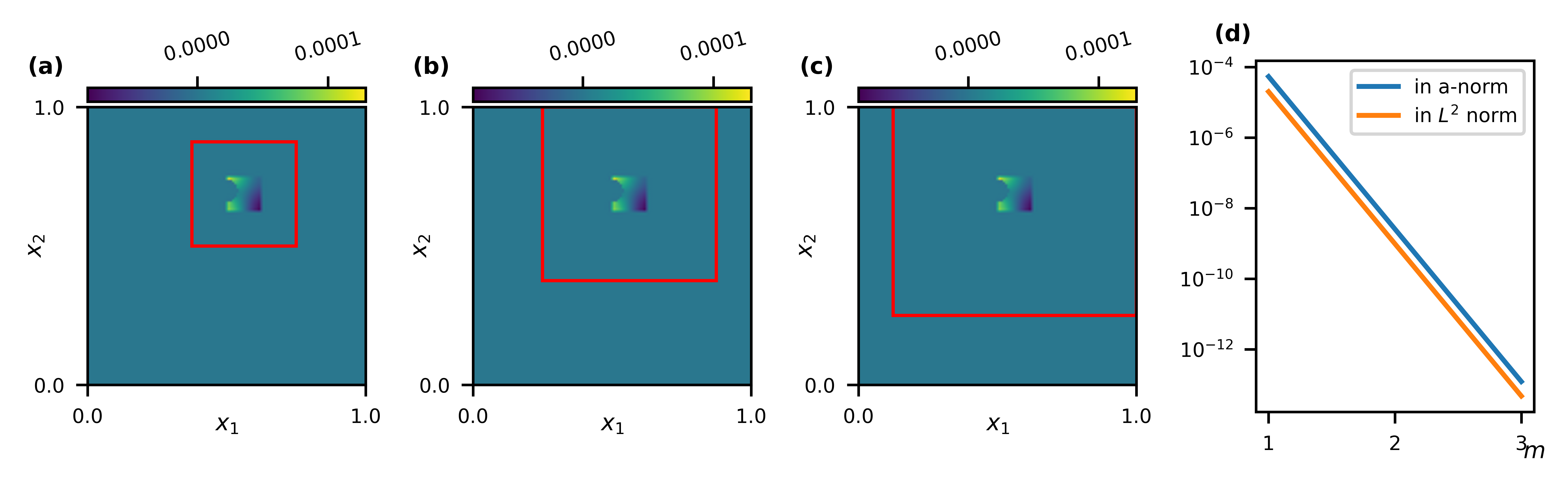
Refer to caption
Figure 5.8: (a) The coefficient profile and the marked coarse element. (b)–(d) The plot of the first/second/third eigenfunction corresponding to the marked coarse element.
Refer to caption
Figure 5.9: (a) multiscale basis function with m=1m=1; (b) multiscale basis function with m=2m=2; (c) multiscale basis function with m=3m=3; (d) Relative differences of the multiscale basis functions with m=1,2,3m=1,2,3 and the global basis functions in the a-norm and L2L^{2} norm.

5.3 2D high-contrast domain

In this section, we consider the Maxwell problem with a high-contrast coefficient μ−1​(x,y)\mu^{-1}(x,y) posed on a two-dimensional suggested in [42, 4] with suitable boundary conditions and source functions. The contrast ratio of the medium is set to Υ=103\Upsilon=10^{3} . To further investigate the performance and scalability of the proposed method, we conduct experiments on progressively refined fine grids, with resolutions up to 2562256^{2} in selected tests. The coarse mesh size HH is chosen from the set {1/32, 1/16, 1/8, 1/4}\{1/32,\,1/16,\,1/8,\,1/4\}.

In this example, we conduct numerical experiments to assess the robustness of the proposed method shown in Figure 5.10. When m=4m=4, the method achieves relative errors on the order of 10−310^{-3} in both the relative L2L^{2} norm and the energy norm for fine coarse meshes, exhibiting clear linear convergence behavior with respect to HH. In Table 5.11, we present detailed CPU time results together with the corresponding numbers of degrees of freedom (DOFs). Based on the linear convergence observed in Fig. 5.10, we fix m=4m=4. For simplicity, only the online stage is reported, using four basis functions per coarse element. As shown in Table 5.11, CEM-GMsFEM reduces the number of DOFs from 131584131584 (FEM) to 40964096 for H=1/32H=1/32, while maintaining a comparable online computational cost. These results demonstrate that the proposed method achieves high accuracy with a substantially reduced system size. These extended tests confirm that the observed linear convergence in HH and exponential decay with respect to mm remain stable under further refinement, while the computational savings in DOFs and online CPU time become more pronounced for larger problem sizes. These results provide stronger evidence of the efficiency and scalability of the proposed CEM-GMsFEM framework.

Refer to caption
Figure 5.10: Subplots (a) and (b) show the relative errors of the proposed method with different numbers of oversampling layers mm w.r.t. the coarse mesh size HH, but measured in different norms.
Table 5.11: Comparison of DOFs and CPU time for the reference solution and the proposed CEM-GMsFEM methods with li=4l_{i}=4.
(m,li)=(4,4)(m,l_{i})=(4,4) Reference solution CEM-GMsFEM solution
h=1/256h=1/256 H=1/32H=1/32 H=1/16H=1/16 H=1/8H=1/8 H=1/4H=1/4
DOFs 131584 4096 1024 256 64
Time (s) 1.361 0.941 0.629 0.055 0.001

6 Conclusions

In this paper, we propose a new multiscale method for solving the Maxwell equations. In the construction of the spectral problem, we introduce a global auxiliary space that eliminates the divergence-free constraint by exploiting the fact that the wave number kk is strictly positive. For locally high-contrast media, the error analysis shows that the proposed multiscale approximation converges to the fine scale solution at a linear rate in the energy norm. Numerical experiments are presented to validate the theoretical convergence results. The extension of the CEM-GMsFEM framework to higher-order convergence and its application to related wave propagation problems are left for future research.

Declaration of competing interest

The authors declare that they have no known competing financial interests or personal relationships that could have appeared to influence the work reported in this paper.

Declaration of Generative AI and AI-assisted technologies in the writing process

During the preparation of this work the authors used ChatGPT in order to improve readability and language. After using this tool, the authors reviewed and edited the content as needed and take full responsibility for the content of the publication.

Acknowledgments

Eric T. Chung’s work is partially supported by the Hong Kong RGC General Research Fund (Project number: 14304525). Part of this work was completed during Xingguang Jin’s visit to the Hausdorff Research Institute for Mathematics at the University of Bonn. He would like to thank Dr. Moritz Hauck for his fruitful discussions and the Hausdorff Research Institute for Mathematics for the support provided through the Hausdorff Fellowship.

References

  • [1] A. Bensoussan, J.-L. Lions, and G. Papanicolaou, Asymptotic analysis for periodic structures, AMS Chelsea Publishing, American Mathematical Society, Providence, RI, (2011). Vol. 374.
  • [2] L. Cao, Y. Zhang, W. Allegretto, and Y. Lin, Multiscale asymptotic method for Maxwell’s equations in composite materials, SIAM J. Numer. Anal. 47 (2010), pp. 4257–4289.
  • [3] E. Chung, Y. Efendiev and T. Y. Hou, Multiscale Model Reduction, Springer, 2023.
  • [4] E. T. Chung, Y. Efendiev and W. T. Leung, Constraint energy minimizing generalized multiscale finite element method, Computer Methods in Applied Mechanics and Engineering. 339 (2018), pp. 298–319.
  • [5] E. T. Chung and Y. Li, Adaptive generalized multiscale finite element methods for H (curl)-elliptic problems with heterogeneous coefficients, J. Comput. Appl. Math. 345 (2019), pp. 357–373.
  • [6] E. T. Chung, C. Ye and X. Zhong, A locking free multiscale method for linear elasticity in stress-displacement formulation with high contrast coefficients, Computer Methods in Applied Mechanics and Engineering. 447 (2025), pp. 118342.
  • [7] E. T. Chung, H. H. Kim and X. Zhong, Iterative contact-resolving hybrid methods for multiscale contact mechanics, Comput. Methods Appl. Mech. Eng. 453 (2026), pp. 118843.
  • [8] P. Ciarlet, S. Fliss, and C. Stohrer, On the approximation of electromagnetic fields by edge finite elements. Part 2: A heterogeneous multiscale method for Maxwell’s equations, Comput. Math. Appl. 73 (2017), pp. 1900–1919.
  • [9] W. E and B. Engquist, The heterognous multiscale methods, Communications in Mathematical Sciences. 1(1) (2003), pp. 87–132.
  • [10] W. E, B. Engquist and Z. Huang, Heterogeneous multiscale method: a general methodology for multiscale modeling, Physical Review B. 67(9) (2003), pp. 092101.
  • [11] Y. Efendiev and T. Y. Hou, Multiscale finite element methods: theory and applications, Springer Science & Business Media. 4 (2009).
  • [12] B. Engquist and Y. H. Tsai, Heterogeneous multiscale methods for stiff ordinary differential equations. Mathematics of computation, Mathematics of computation. 74(252) (2005), pp. 1707–1742.
  • [13] J. Galvis and Y. Efendiev, Domain decomposition preconditioners for multiscale flows in high-contrast media, SIAM Multiscale Modeling & Simulation. 8(4) (2010), pp. 1461–1483.
  • [14] P. Henning, M. Ohlberger, and B. Verfürth, A new heterogeneous multiscale method for time-harmonic Maxwell’s equations, SIAM J. Numer. Anal. 54 (2016), pp. 3493–3522.
  • [15] P. Henning and A. Persson, Computational homogenization of time-harmonic Maxwell’s equations, SIAM Journal on Scientific Computing. 42(3) (2020), pp. B581–B607.
  • [16] R. Hiptmair, Finite elements in computational electromagnetism, Acta Numer. 11 (2002), pp. 237–339.
  • [17] M. Hochbruck and C. Stohrer, Finite element heterogeneous multiscale method for time dependent Maxwell’s equations, in Spectral and High Order Methods for Partial Differential Equations—ICOSAHOM 2016, Lect. Notes Comput. Sci. Eng. 119 (2017), pp. 269–281.
  • [18] C. L. Holloway, A. Dienstfrey, E. F. Kuester, J. F. O’Hara, A. K. Azad, and A. J. Taylor, A discussion on the interpretation and characterization of metafilms/metasurfaces: The two-dimensional equivalent of metamaterials, Metamaterials. 3(2) (2009), pp. 100–112.
  • [19] T. Y. Hou and X. H. Wu, A multiscale finite element method for elliptic problems in composite materials and porous media, Journal of computational physics. 134(1) (1997), pp. 169–189.
  • [20] T. J. Hughes, G. R. Feijóo, L. Mazzei, and J. B. Quincy, The variational multiscale method—a paradigm for computational mechanics, Computer methods in applied mechanics and engineering. 166(1-2) (1998), pp. 3–24.
  • [21] S. G. Johnson, S. Fan, P. R. Villeneuve, J. D. Joannopoulos, and L. A. Kolodziejski, Guided modes in photonic crystal slabs, Phys. Rev. B 60 (1999), pp. 5751–5758.
  • [22] A. Lamacz and B. Schweizer, A negative index meta-material for Maxwell’s equations, SIAM J. Math. Anal. 48(6) (2016), pp. 4155–4174.
  • [23] U. Leonhardt, Optical conformal mapping, Science 312(5781) (2006), pp. 1777–1780.
  • [24] R. Lipton and B. Schweizer, Effective Maxwell’s equations for perfectly conducting split ring resonators, Arch. Ration. Mech. Anal. 229(3) (2018), pp. 1197–1221.
  • [25] C. Ma and Y. Zhang, Multiscale model reduction and two-level Schwarz preconditioner for H(curl) elliptic problems, preprint, arXiv:2506.07381 (2025).
  • [26] A. Målqvist and D. Peterseim, Localization of elliptic multiscale problems, Mathematics of Computation. 83(290) (2014), pp. 2583–2603.
  • [27] R. D. Meade, S. G. Johnson, and J. N. Winn, Photonic crystals: Molding the flow of light, Princeton University Press, Princeton, NJ, (2008).
  • [28] P. Monk, Finite element methods for Maxwell’s equations, Oxford university press. (2003).
  • [29] J. B. Pendry, Negative refraction makes a perfect lens, Phys. Rev. Lett. 85(18) (2000), pp. 3966.
  • [30] J. B. Pendry, A. J. Holden, D. J. Robbins, and W. J. Stewart, Magnetism from conductors and enhanced nonlinear phenomena, IEEE Transactions on Microwave Theory and Techniques. 47(11) (1999), pp. 2075–2084.
  • [31] D. Peterseim, Eliminating the pollution effect in Helmholtz problems by local subscale correction, Mathematics of Computation. 86(305) (2017), pp. 1005–1036.
  • [32] D. Peterseim, and R. Scheichl, Robust numerical upscaling of elliptic multiscale problems at high contrast, Computational Methods in Applied Mathematics. 16(4) (2016), pp. 579–603.
  • [33] K. Sakoda, Optical properties of photonic crystals, Springer, Berlin, Heidelberg, (2005).
  • [34] D. R. Smith, J. B. Pendry, and M. C. Wiltshire, Metamaterials and negative refractive index, Science 305(5685) (2004), pp. 788–792.
  • [35] B. Verfürth, Heterogeneous multiscale method for the Maxwell equations with high contrast, ESAIM: Math. Model. Numer. Anal. 53(1) (2019), pp. 35–61.
  • [36] V. G. Veselago, The electrodynamics of substances with simultaneously negative values of ε\varepsilon and μ\mu, Uspekhi Fizicheskikh Nauk. 92(3) (1967), pp. 517–526.
  • [37] Y. Wang, W. T. Leung, and G. Li, Numerical homogenization for indefinite time-harmonic Maxwell equations, arXiv preprint arXiv:2604.22502 (2026).
  • [38] C. Ye, X. Jin, P. Ciarlet Jr., and E. T. Chung, Multiscale modeling for a class of high-contrast heterogeneous sign-changing problems, preprint, arXiv:2407.17130 (2024).
  • [39] Y. Zhou, X. Zhong, C. Ye and E. T. Chung, Efficient Multiscale Methods for Highly Heterogeneous Spatial Network Models, arXiv preprint arXiv:2605.09280 (2026).
  • [40] X. Jin, L. Liu, X. Zhong, and E. T. Chung, Efficient numerical method for the Schrödinger equation with high-contrast potentials, SIAM Multiscale Modeling & Simulation. 23(4) (2025), pp. 1581–1606.
  • [41] W. Xie, E. T. Chung, Y. Yang, and Y. Huang, Adaptive multiscale model reduction for linear elasticity equation in perforated domains, arXiv preprint arXiv:2606.06839, 2026.
  • [42] E. T. Chung, P. Ciarlet Jr., X. Jin, and C. Ye, Multiscale Methods for wave propagation in materials with sign-changing coefficients, arXiv preprint arXiv:2511.20103, 2026.