Scaling in Supersonic Turbulence: Energy Spectra and Fluxes using High-Fidelity Direct Numerical Simulations

The governing equations are the compressible Navier-Stokes equations, solved in the nondimensional form. The equations can be represented using tensorial notations as given below [23]:

where $\rho$, $\mathbf{u}$, $p$, $T$, and $\mathbf{F}$ denote the density, velocity, pressure, temperature, and external force field, respectively. The viscous stress tensor $\tau_{ij}$ is defined as

where $\mathrm{Re}_{0}$ is the reference Reynolds number. The heat flux $q_{i}$ is given by Fourier’s law:

The total energy density $E_{T}$ is composed of the kinetic energy density $E_{u}$ and internal energy density $I$:

We solve Eqs. (1-3) using finite volume method on a structured uniform Cartesian grids. All the equations are written in vectorial notation in the following conservative form [48]:

where $\mathbf{X}$ is a column vector that contains the variables $\rho$, $\rho u_{\beta}$, and $E_{T}$, and the index $\beta=1,2,3$ represent the $x$, $y$, and $z$ directions respectively. Here, $\mathbf{F}^{\beta}$ represents the nonlinear convection flux in the $\beta$-direction, $\mathbf{G}^{\beta}$ is the corresponding viscous flux, and $\mathbf{S}$ is the source term. Hence,

The convective fluxes are evaluated using the semidiscrete central scheme of Kurganov and Tadmor [49, 50], which avoids the need for Riemann solvers while retaining robustness near discontinuities. In the $x$-direction, the reconstructed left ($q^{-}_{i+1/2,j,k}$) and right ($q^{+}_{i+1/2,j,k}$) states are used to compute the numerical flux,

where $a_{i+1/2,j,k}$ is the local maximum propagation speed in $x$-direction determined from the eigenvalues of the Jacobian flux. Identical processes are also adopted for the $y$- and $z$-directions. The viscous fluxes $\mathbf{G}^{\beta}$ are discretized using fourth-order central difference schemes. Time integration is performed using the explicit third-order Strong Stability Preserving Runge-Kutta (eSSPRK3) method [51]. The timestep $\Delta t$ is dynamically adjusted according to the Courant–Friedrichs–Lewy (CFL) condition,

where $C_{0}$ is CFL number and $\Lambda_{\beta}$ are the spectral radii of the Jacobian flux in the $\beta$ directions.

In the seminal work of Kurganov and Tadmor [49], a linear reconstruction of the cell-average was used to compute left and right interface states. To achieve high-order spatial accuracy, we tested several nonlinear reconstruction schemes that are widely used in the literature, including Weighted Essentially Non-Oscillatory (WENO) [52, 53], Central WENO (CWENO) [54, 50] and Targeted Essentially Non-Oscillatory (TENO) [46] schemes. Classical WENO formulations, such as WENO-JS [52], can be overly dissipative in smooth flow regions. To mitigate this, we initially considered WENO-Z [53], which utilizes global smoothness indicators to reduce dissipation. However, we ultimately adopted the TENO scheme, which replaces the weighted stencil averaging of WENO with a threshold-based cutoff strategy to sharply discard non-smooth stencils [46]. The numerical methods described are implemented using the high-performance Python fluid solver DHARA [47]. In Appendix  A, benchmark tests for various high-order reconstruction schemes are briefly presented for 3D compressible Taylor-Green Vortex (§ A.1), Isentropic Vortex (§ A.2), and Kelvin-Helmholtz instability (§ A.3). For all these cases, we found the seventh-order Targeted Essentially Non-Oscillatory (TENO7) scheme to be the most accurate, exhibiting the lowest dissipation while maintaining robustness.

Designed for modern supercomputers, DHARA leverages CuPy [55] for seamless GPU acceleration via NVIDIA CUDA, achieving a speedup of around $150X$ on a single NVIDIA A100 GPU compared to a single-core AMD EPYC 7543 CPU. The solver demonstrates excellent scalability on systems like Frontier (Oak Ridge National Laboratory) and Polaris (Argonne National Laboratory), showing strong scaling and good weak scaling across multiple nodes (see Appendix A).

The simulations are performed at six turbulent Mach numbers, $M_{t}=0.2,0.7,1.0,1.4,1.8$ and $3.0$. To sustain turbulence, we apply external stochastic forcing following an Ornstein–Uhlenbeck process, as detailed in § II.1.2. We inject energy in the wavenumber range $1\leq k\leq 3$, with the peak amplitude at $k_{0}=2$. The forcing is governed by two parameters: the projection parameter $\zeta$, which determines the degree of compressibility, and the amplitude $U_{0}$, which controls the root-mean-square velocity. For the simulations with $M_{t}=0.2,1.0,1.8,$ and $3.0$, we employ predominantly solenoidal driving ($\zeta=2/3$) with amplitudes $U_{0}=0.02$, $0.1$, $0.2$ and $0.3$ respectively. Conversely, for the $M_{t}=0.7$ and $1.4$ runs, we use a more compressively weighted forcing ($\zeta=1/3$) with $U_{0}=0.1$ and $0.2$, respectively. These parameters were selected to study steady-state turbulence across a range of $M_{t}$ and investigate the effects of varying compressibility in the external driving.

We choose $\gamma=1.00001$, making the flow nearly isothermal. This ensures a statistically stationary state by preventing viscous dissipation from monotonically increasing the internal energy and reducing the Mach number. In addition, the nondimensionalized gas constant $R^{*}=1/(\gamma M_{0}^{2})\approx 0.01$ leads to $\sigma\approx 0.01\rho T$ and $I=\sigma/(\gamma-1)\approx 10^{3}$. This models astrophysical flows with efficient radiative cooling, such as supersonic turbulence in the interstellar medium and molecular clouds. The other simulation parameters are set as $Pr=1$ and $M_{0}=10$. In each simulation, the flow is initialized with uniform density and temperature, $\rho(t=0)=T(t=0)=1$, and zero velocity $\mathbf{u}(t=0)=0$. The simulations are evolved for more than 40 eddy turnover times, $t_{\text{eddy}}=l_{0}/u_{0}$, to ensure statistical convergence. To speed up convergence and reduce initial transients, we first evolve the system on a coarser $512^{3}$ grid until it reaches a statistically steady state. The resulting field is then interpolated onto a finer $1024^{3}$ grid for further evolution. Each high-resolution run was performed on the Polaris supercomputer with 32 nodes (128 A100 GPUs). The highest Mach number run $M_{t}=3.0$, required approximately 60 hours of computation time.

Table 1 summarizes the key parameters for the these simulations, including the forcing parameter $\zeta$, characteristic velocity scale $U_{0}$, energy injection rates $(\epsilon^{\mathrm{inj}}_{R},\epsilon^{\mathrm{inj}}_{C})$, Taylor microscale Reynolds number $\mathrm{Re}_{\lambda}$, steady-state turbulent Mach number $M_{t}$, and the Kolmogorov scale resolution ratio $\eta/\Delta x$. Here, $\eta=\left[{\langle\mu\rangle^{3}}/({\epsilon\langle\rho\rangle^{2})}\right]^{1/4}$ is the Kolmogorov length scale, with $\langle\mu\rangle$ and $\langle\rho\rangle$ denoting volume-averaged dynamic viscosity and density, and $\epsilon$ the average energy dissipation rate [30]. We verify that all runs are well-resolved, satisfying the standard resolution criterion $\eta/\Delta x\geq 1$ (see Table 1).

All simulations were integrated for more than 40 eddy turnover times. For our analysis, we discard the initial transients and focus on the statistically stationary state. Figure 1 presents the time series of the total kinetic energy, $E_{u}$, and the maximum local Mach number, $M_{t,\mathrm{max}}$, over 20 eddy turnover times within this stationary regime. As shown, $E_{u}$ remains nearly stable, whereas $M_{t,\mathrm{max}}$ exhibits large fluctuations above the mean. These deviations reflect intermittent bursts of intense compression and strong localized shocks.

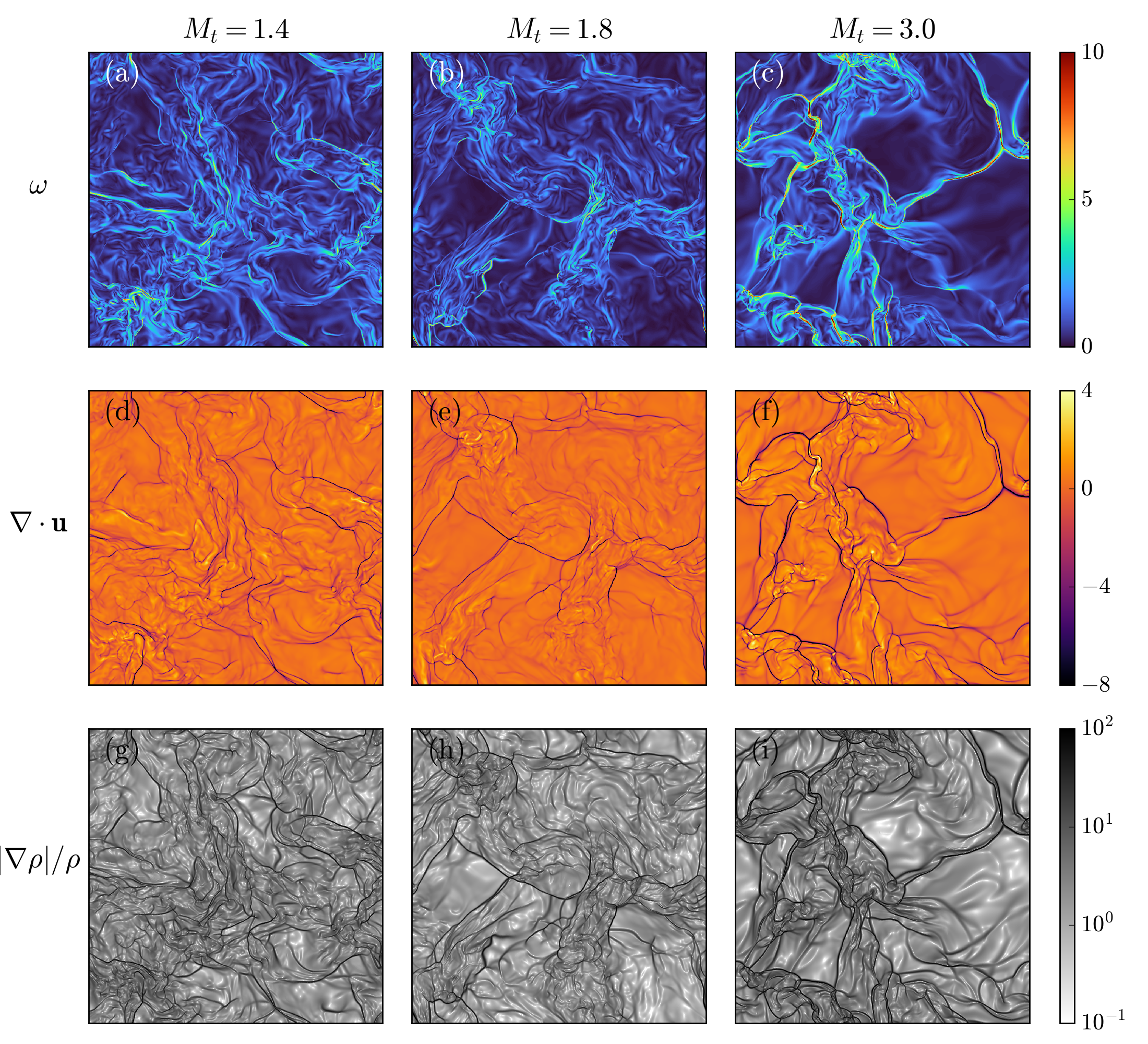
Figures 2 and 3 display instantaneous $x$–$z$ cross-sections of the vorticity magnitude $\omega=|\nabla\times\mathbf{u}|$ (top row), velocity divergence $\nabla\cdot\mathbf{u}$ (middle row), and normalized density gradient magnitude $|\nabla\rho|/\rho$ (bottom row) in the statistically stationary state. Figure 2 corresponds to the subsonic and transonic cases ($M_{t}=0.2,0.7,1.0$), while Fig. 3 presents the supersonic runs ($M_{t}=1.4,1.8,3.0$); for movies, see Ref. [56]. The divergence fields highlight regions of intense compression, where large negative values of $\nabla\cdot\mathbf{u}$ correspond to local Mach numbers significantly exceeding $M_{t}$. These sharp discontinuities are similarly captured by the density gradients, which effectively resolve the widths of the simulated shocks.

The progression from $M_{t}=0.2$ to $M_{t}=3.0$ demonstrates the effects of turbulent Mach number and forcing composition on the structural evolution of compressible turbulence. As $M_{t}$ increases, the magnitudes of both $\nabla\cdot\mathbf{u}$ and $|\nabla\rho|/\rho$ rise significantly, signalling a progressive strengthening of the shock structures. In the nearly incompressible limit ($M_{t}=0.2$), such structures are virtually absent. However, in the subsonic and transonic cases, the flow is characterized by fragmented shocklets distributed throughout the domain. In the supersonic simulations, these features evolve into strong, persistent shock sheets. The density gradients further highlight these sharp discontinuities—representing the numerical shock widths—where density jumps of several orders of magnitude occur within just a few grid cells. These structures are consistent with previous investigations of high-Mach-number turbulence [9, 11].

In the subsonic regime, the vorticity field is filled by fine-scale structures distributed throughout the domain, a consequence of the high Reynolds numbers ($Re_{\lambda}$). As $M_{t}$ increases, however, the spatial organization changes. Notably, regions of intense vorticity become increasingly concentrated in the vicinity of shock structures. This localization arises because vorticity is generated via baroclinic torque at curved shock fronts and subsequently amplified by vortex stretching, where solenoidal cascades develop from compressive seeds [24, 11].

To compute energy spectra and fluxes, we employ the mode-to-mode formalism developed in [43]. Using the Helmholtz decomposition, we decompose the velocity field into rotational ($\alpha=R$) and compressible ($\alpha=C$) components, denoted by $\mathbf{u}_{\alpha}(\mathbf{k})$. The corresponding density-weighted velocity fields are defined as $\mathbf{v}_{\alpha}(\mathbf{k})$, where $\mathbf{v}(\mathbf{x})=\rho(\mathbf{x})\,\mathbf{u}(\mathbf{x})$. The kinetic energy for each mode is given by

yielding the total kinetic energy spectrum

In addition to the kinetic energy spectra, the density spectrum is defined as [57, 58]

We compute the kinetic energy (KE) spectra for the rotational and compressive velocity components, $E_{R}(k)$ and $E_{C}(k)$, the total kinetic energy spectrum $E_{u}(k)$, and the density spectrum $E_{\rho}(k)$, averaged over 20 snapshots. Figure 4 presents these spectra for $M_{t}=0.2$, $0.7$ and $1.0$, while Fig. 5 displays the results for $M_{t}=1.4,1.8$, and $3.0$. The errors in the spectral exponents are less than $1\%$. In the nearly incompressible limit ($M_{t}=0.2$), both kinetic energy and density spectra scale as $k^{-5/3}$, consistent with the results of  Zank and Matthaeus [31]. For the subsonic and transonic cases ($M_{t}=0.7$ and $1.0$), the rotational spectrum retains Kolmogorov scaling ($E_{R}(k)\sim k^{-5/3}$), whereas the compressive component exhibits a Burgers-like $k^{-2}$ scaling. The density spectrum similarly follows this $k^{-2}$ behavior. These observations are consistent with established findings for subsonic turbulence [23, 32, 33, 34, 58].

In contrast, the energy distribution changes significantly in the supersonic regime ($M_{t}=1.4,1.8$, and $3.0$). With increasing $M_{t}$, $E_{R}(k)$ steepens, deviating from the Kolmogorov $k^{-5/3}$ law and approaching a Burgers-like $k^{-2}$ slope at $M_{t}=3.0$, despite the use of predominantly solenoidal forcing. Furthermore, while $E_{C}(k)$ follows $k^{-2}$ at $M_{t}=1.4$, it becomes progressively shallower at higher Mach numbers. These results contrast with the shallower scaling for both rotational and compressive KE ($E_{\alpha}(k)\sim k^{-3/2}$) reported by Kritsuk et al. [9] and Federrath et al. [35]. We note, however, that those studies defined the kinetic energy as $w^{2}/2$, where $\mathbf{w}=\sqrt{\rho}\,\mathbf{u}$ is the density-weighted velocity. The density spectrum also flattens with increasing $M_{t}$, approaching $k^{-1}$ at $M_{t}=3.0$, which agrees with high Mach number results in the literature [9, 35]. In all cases, the total kinetic energy remains close to the solenoidal spectrum. These results demonstrate the stark difference in energy distribution at different scales between supersonic and subsonic turbulence.

Now, we report the various energy fluxes in the flow and assess the effect of compressibility in energy cascade. Following the formalism of Singh et al. [43], the spectral evolution of the kinetic energy for the rotational ($\alpha=R$) and compressive ($\alpha=C$) modes is governed by

where ${\bf k=p+q}$. The first term on the right-hand side is the mode-to-mode energy transfer from ${\bf u}_{\alpha}({\bf p})$ to ${\bf u}_{\alpha}({\bf k})$. It represents the non-linear exchange of energy within the rotational modes (via $S^{RR}$) or within the compressive modes (via $S^{CC}$). The interaction between different kinetic energy components is described by the cross-transfer term $S^{\alpha\beta}$, which quantifies the energy exchanged between rotational and compressive modes. Additionally, ${\bf u}_{\alpha}({\bf k})$ exchanges energy with internal energy via pressure work $Q_{I,\alpha}(\mathbf{k})$ and viscous dissipation $D_{I,\alpha}(\mathbf{k})$. $\mathcal{F}_{\alpha}(\mathbf{k})$ is the kinetic energy injection rate by the external force component. These terms are defined as

In these expressions, $p(\mathbf{k})$ represents the Fourier amplitude of the pressure, and $\mathbf{F}_{\alpha}(\mathbf{k})$ denotes the Fourier amplitudes of the rotational and compressible forcing components. The remaining quantities are defined as

where $\tau_{ij}$ denotes the viscous stress tensor.

We define different energy fluxes corresponding to these transfer terms. To quantify interscale energy transfer, we define the pure flux

which measures the net rate of energy transfer from $\alpha$-modes (rotational/compressible) within a wavenumber sphere of radius $K$ to $\alpha$-modes (rotational/compressible) outside the sphere. Physically, $\Pi_{R}$ represents the traditional Kolmogorov-like cascade where large-scale solenoidal eddies break down into smaller vortical structures. In contrast, $\Pi_{C}$ represents the acoustic or shock-like cascade, where large-scale compressions steepen into small-scale shocklets or shock sheets. Similarly, the cross-flux

represents the net transfer from $\alpha$-modes inside the sphere to all $\beta$-modes, allowing us to track exchanges between solenoidal and compressible motions. For example, $\Pi^{R<}_{C}$ quantifies how the deformation of rotational eddies acts as a source for new compressive structures at all scales. The energy exchanges between $E_{u}$ and $I$ are captured through fluxes associated with $Q$ and $D$:

We also define the rotational and compressive average dissipation rates as

For the definition of the mode-to-mode transfer functions and further details, see [43], which form the basis of the flux definitions used in this study.

The fluxes are normalized using

where $\epsilon$ is the average dissipation rate and $\mathcal{W}=\langle-p\,\nabla\cdot\mathbf{u}\rangle$ denotes the average pressure–dilatation. The quantity $\epsilon_{T}$ therefore equals the total energy injection rate ($\epsilon^{\mathrm{inj}}$) at steady state, or equivalently, the net rate of kinetic–to–internal energy conversion [24]. We denote the normalized fluxes and energy injection rates with tildes (e.g., $\tilde{\Pi}_{R}(k)$ vs. ${\Pi}_{R}(k)$) to distinguish them from their unnormalized forms.

We compute the normalized energy fluxes, averaged over 15–20 snapshots at steady state. Figure 4 (b,c,e,f,h,i) presents these fluxes for the subsonic and transonic regimes ($M_{t}=0.2,0.7,1.0$), while Fig. 6(a–c) further illustrates the energy transfer pathways. In the nearly incompressible limit ($M_{t}=0.2$), the rotational flux $\tilde{\Pi}_{R}(k)$ remains constant across the inertial range. The compressive flux $\tilde{\Pi}_{C}(k)$, cross-fluxes, and pressure dilatation are negligible, consistent with ideal incompressible dynamics. In the subsonic regime ($M_{t}=0.7$), both $\tilde{\Pi}_{R}(k)$ and $\tilde{\Pi}_{C}(k)$ exhibit constant plateaus in the inertial range ($4\lessapprox k\lessapprox 15$) [32, 59]. The cross-transfer is weak ($\tilde{\Pi}^{R<}_{C}(k)\approx 0.1$) and confined to large scales. Consequently, it has a negligible impact on the inertial-range fluxes [60]. Interestingly, in the transonic case ($M_{t}=1.0$), although the cross-flux strengthens significantly ($\tilde{\Pi}^{R<}_{C}(k)\approx 0.3$), it remains restricted to small wavenumbers. As a result, both $\tilde{\Pi}_{R}(k)$ and $\tilde{\Pi}_{C}(k)$ maintain their constant, cascade-like behavior in the inertial range even in the transonic case. For both $M_{t}=0.7$ and $1.0$, pressure dilatation $\tilde{\Pi}^{C<}_{I,Q}(k)$ becomes comparable to the compressive viscous dissipation. However, it remains nearly constant at intermediate and large wavenumbers, indicating that energy transfer via pressure work occurs primarily at large scales [37]. In contrast, the pressure contribution to the rotational component, $\tilde{\Pi}^{R<}_{I,Q}(k)$, remains negligible.

The energy transfer in supersonic flows differs significantly from that in the subsonic and transonic regimes. Figure 5(b,c,e,f,h,i) presents these fluxes for supersonic turbulence, with rows corresponding to $M_{t}=1.4$, $1.8$, and $3.0$. Additionally, Fig. 6(d–f) illustrates the energy transfer pathways. The key features of the normalized fluxes are as follows:

• •

  Rotational component: Energy injected into rotational modes, $\tilde{\epsilon}^{\mathrm{inj}}_{R}$, splits into two pathways: a forward cascade, $\tilde{\Pi}_{R}$, and a cross-transfer to compressible modes, $\tilde{\Pi}^{R<}_{C}$. In contrast to the subsonic case, a significant fraction of $\tilde{\epsilon}^{\mathrm{inj}}_{R}$ is transferred to the compressible modes in supersonic turbulence. Although this transfer is most active at large scales, $\tilde{\Pi}^{R<}_{C}$ continues to grow across the intermediate scales, indicating substantial cross-transfer within the inertial range. Consequently, the energy available for the forward cascade diminishes, causing $\tilde{\Pi}_{R}$ to decrease with $k$. This behavior contrasts sharply with the Kolmogorov-like constant flux observed in subsonic turbulence. As a result, the rotational spectrum $E_{R}(k)$ steepens, deviating from $k^{-5/3}$ scaling. Figure 6 confirms that increasing $M_{t}$ amplifies $\tilde{\Pi}^{R<}_{C}$, driving the steepening of both $\tilde{\Pi}_{R}$ and $E_{R}(k)$. We also note that $\tilde{\Pi}^{R<}_{C}$ depends on the forcing parameter $\zeta$, remaining lower for mixed forcing than for predominantly solenoidal forcing at similar Mach numbers.
  

• •

  Compressive component: Figure 6 shows that the compressible modes gain energy from two sources: direct forcing, $\tilde{\epsilon}^{\mathrm{inj}}_{C}$, and cross-transfer from rotational modes, $-\tilde{\Pi}^{C<}_{R}$. This energy splits into two paths: (a) a forward cascade to smaller scales via $\tilde{\Pi}_{C}(k)$, and (b) conversion to internal energy via pressure dilatation, $\tilde{\Pi}^{C}_{I,Q}(k)$. As seen in Fig. 5(b,e,h), $\tilde{\Pi}_{C}(k)$ increases slightly across the inertial range. This occurs because the cross-transfer adds energy even at intermediate scales, increasing the energy available for the forward transfer. Consequently, $\tilde{\Pi}_{C}(k)$ rises across the inertial range. This leads to a shallower compressive spectrum, particularly at higher $M_{t}$. However, the rise in $\tilde{\Pi}_{C}(k)$ is much weaker than the steepening of $\tilde{\Pi}_{R}(k)$ because a portion of the transferred energy is converted to internal energy via pressure dilatation.
  

  

• •

  Pressure dilatation: Pressure dilatation converts kinetic energy to internal energy via pressure work. Figure 6 shows that this work is significant for the compressive component and remains comparable to the compressive viscous dissipation. Notably, the compressive pressure dilatation increases with increasing $M_{t}$. Figure 5(c,f,i) reveals that the compressive pressure dilatation flux, $\tilde{\Pi}^{C<}_{I,Q}(k)$, is most active at large scales (small $k$). However, unlike the subsonic case, it retains a non-negligible magnitude throughout the inertial range. In contrast, the pressure flux for the rotational component vanishes ($\tilde{\Pi}^{R<}_{I,Q}\rightarrow 0$). This aligns with incompressible theory, where pressure does not contribute to energy transfers [61, 16, 62].
  

• •

  Viscous dissipation: Viscous dissipation irreversibly converts kinetic energy into internal energy. The maximum of viscous flux, $\tilde{\Pi}^{\alpha<}_{I,D}(k)$, matches the total dissipation rate $\tilde{\epsilon}_{\alpha}$. As shown in Fig. 5(c,f,i), $\tilde{\Pi}^{\alpha<}_{I,D}(k)$ increases gradually with wavenumber $k$ for each component. This indicates that dissipation is active across all scales, though predominantly at small scales. Interestingly, the compressive dissipation spectrum exhibits small negative values at low wavenumbers, implying a reverse energy transfer from internal to compressive modes. This behavior arises from the density-weighted formulation of the viscous divergence [43] and intensifies at higher $M_{t}$. Despite this local reversal, the total compressive dissipation remains positive. Figure 6 demonstrates that as $M_{t}$ increases, the total rotational viscous dissipation decreases, whereas the compressive dissipation increases.

We summarize the variation of key turbulent statistics with turbulent Mach number ($M_{t}$) in Table 2 and Fig. 7. The simulations comprise two subsets: a primarily rotational forcing ($\zeta=2/3$ for $M_{t}=0.2,1.0,1.8,3.0$) and a mixed forcing ($\zeta=1/3$ for $M_{t}=0.7,1.4$). The normalized injection rates ($\tilde{\epsilon}^{\mathrm{inj}}_{R},\tilde{\epsilon}^{\mathrm{inj}}_{C}$) show little variation with $M_{t}$ but depend strongly on the forcing parameter $\zeta$, which controls the ratio of rotational to compressive forcing amplitudes. For runs with $\zeta=2/3$, the rotational injection rate $\tilde{\epsilon}^{\mathrm{inj}}_{R}$ ranges from $0.93$ to $0.98$, while for $\zeta=1/3$, it drops to approximately $0.76$. Despite the relatively constant injection rates for a given $\zeta$, the flow composition changes significantly with increasing $M_{t}$. For instance, within the fixed $\zeta=2/3$ subset, the ratio of rotational to compressive kinetic energy ($E_{R}/E_{C}$) drops from 322.3 to 6.12 as $M_{t}$ increases, indicating that compressibility becomes increasingly dominant as the Mach number rises.

While the energy injection at large scales is forcing-dependent, the subsequent energy transfers and spectral scaling exhibit a clear, monotonic dependence on $M_{t}$, indicating that these dynamics are predominantly governed by the Mach number rather than the forcing composition. Figure 7(a) elucidates this trend. As $M_{t}$ increases, the normalized rotational dissipation $\tilde{\epsilon}_{R}$ decreases, while the cross-transfer flux from rotational to compressive modes, $\tilde{\Pi}^{R}_{C}$, rises markedly from 0.02 to 0.70. This confirms that in supersonic flows, a significant fraction of solenoidal energy is transferred into the compressive modes rather than being dissipated by viscosity. It is important to note from Fig. 4 and Fig. 5 that while the fluxes $\Pi^{R<}_{C}$ and $-\Pi^{C<}_{R}$ do not strictly match at every scale, their total integrated transfers are identical (see Table 2), representing the net total transfer from rotational to compressive modes. For the compressive modes [Fig. 7(b)], both the compressive dissipation $\tilde{\epsilon}_{C}$ and total compressive pressure dilatation $\tilde{\Pi}^{C}_{I,Q}$ increase with $M_{t}$, converting compressive kinetic energy into internal energy. Notably, $\tilde{\epsilon}_{C}$ and $\tilde{\Pi}^{C}_{I,Q}$ remain comparable across the entire Mach number range, with the exception of the near-incompressible limit ($M_{t}=0.2$). These dynamical changes directly influence the spectral scaling exponents ($\alpha$) listed in Table 2, where the rotational and total velocity spectra steepen due to the energy drain via cross-transfer flux. In contrast, the compressive velocity spectrum shallows at higher Mach numbers. Consistent with previous studies [9, 35], the density spectrum approaches $k^{-1}$ at high $M_{t}$. It is worth noting that while these energy-cascade trends appear robust across our current setup, the specific energy-transfer rates may exhibit a stronger dependence on forcing in different parameter regimes.

Burgers equation is [63]

where $\nu$ is the kinematic viscosity. It represents fully compressible fluid with no pressure term. In Burgers turbulence, the energy spectrum follows

where $\Delta V$ is the velocity jump across the shock and $L$ is the domain size [64, 65]. Saffman [64] further established that the RMS velocity ($U_{B}$) and the energy flux ($\Pi_{B}$) scale with $\Delta V$ as

Now, we compare the above predictions with our numerical results.

In our simulation, we calculated $\Delta V$ by identifying velocity jumps across shocks in the $u_{x}$ component for a fixed $y$ and then averaging their magnitudes over a sample of 20 distinct spatial coordinates ($z$) and 20 time snapshots. This process provides good spatial and temporal averaging. This yield $\Delta V=0.08$, 0.11, 0.15, 0.19 and 0.30 for $M_{t}=0.7$, 1.0, 1.4, 1.8 and 3.0 respectively. The uncertainties in calculating $\Delta V$ is around 0.02. The estimates for $\Delta V$ are close to rms velocity ($U=cM_{t}$). For illustration, in Fig. 8(a) we exhibit $u_{x}(x,y=\pi,z=\pi)$ for three different snapshots of the $M_{t}=3.0$ run. The figure shows that the velocity differences across shocks are of the order of $U$.

Figure 8(b) presents the rotational and compressive RMS velocities ($U_{R}$, $U_{C}$ ) and the maximum energy fluxes ($\Pi_{R}$, $\Pi_{C}$). The compressive components align remarkably well with Burgers equation predictions (solid and dashed black lines). A best-fit analysis yields

Interestingly, the rotational component exhibits similar scaling trends with respect to the shock strength $\Delta V$:

The physical mechanisms underlying these rotational scaling laws remain to be fully understood and need further investigation. The above discussion brings out interesting connections between the Burgers turbulence and compressible turbulence. We believe that Eqs. (42, 43) can play a very important role in modelling complex astrophysical flows with high Mach numbers.

References

- Carroll [2006] B. W. Carroll, An Introduction to Modern Astrophysics, 2nd ed. (Pearson, 2006).
- Elmegreen and Scalo [2004] B. G. Elmegreen and J. Scalo, Interstellar turbulence I: Observations and processes, Annu. Rev. Astron. Astrophys. 42, 211 (2004).
- Mac Low and Klessen [2004] M.-M. Mac Low and R. S. Klessen, Control of star formation by supersonic turbulence, Reviews of modern physics 76, 125 (2004).
- von Kármán [1941] T. von Kármán, Compressibility effects in aerodynamics, Journal of the Aeronautical Sciences 8, 337 (1941).
- Krumholz and McKee [2005] M. R. Krumholz and C. F. McKee, A general theory of turbulence-regulated star formation, from spirals to ultraluminous infrared galaxies, Astrophys. J. 630, 250 (2005).
- Padoan and Nordlund [2011] P. Padoan and Å. Nordlund, The star formation rate of supersonic magnetohydrodynamic turbulence, Astrophys. J. 730, 40 (2011).
- Fujisawa [2021] A. Fujisawa, Review of plasma turbulence experiments, Proc. Jpn. Acad., Ser. B 97, 103 (2021).
- Ingenito and Bruno [2010] A. Ingenito and C. Bruno, Physics and regimes of supersonic combustion, AIAA journal 48, 515 (2010).
- Kritsuk et al. [2007] A. G. Kritsuk, M. L. Norman, P. Padoan, and R. Wagner, The statistics of supersonic isothermal turbulence, Astrophys. J. 665, 416 (2007).
- Schmidt et al. [2009] W. Schmidt, C. Federrath, M. Hupp, S. Kern, and J. C. Niemeyer, Numerical simulations of compressively driven interstellar turbulence-i. isothermal gas, Astron. Astrophys. 494, 127 (2009).
- Federrath [2013] C. Federrath, On the universality of supersonic turbulence, Mon. Not. R. Astron. Soc. 436, 1245 (2013).
- Kolmogorov [1941a] A. N. Kolmogorov, Dissipation of Energy in Locally Isotropic Turbulence, Dokl Acad Nauk SSSR 32, 16 (1941a).
- Kolmogorov [1941b] A. N. Kolmogorov, The local structure of turbulence in incompressible viscous fluid for very large Reynolds numbers, Dokl Acad Nauk SSSR 30, 301 (1941b).
- Kraichnan [1959] R. H. Kraichnan, The structure of isotropic turbulence at very high Reynolds numbers, J. Fluid Mech. 5, 497 (1959).
- Dar et al. [2001] G. Dar, M. K. Verma, and V. Eswaran, Energy transfer in two-dimensional magnetohydrodynamic turbulence: formalism and numerical results, Physica D 157, 207 (2001).
- Verma [2004] M. K. Verma, Statistical theory of magnetohydrodynamic turbulence: recent results, Phys. Rep. 401, 229 (2004).
- Lesieur [2008] M. Lesieur, Turbulence in Fluids (Springer-Verlag, Dordrecht, 2008).
- Kraichnan [1971] R. H. Kraichnan, Inertial-range transfer in two-and three-dimensional turbulence, J. Fluid Mech. 47, 525 (1971).
- Domaradzki and Rogallo [1990] J. A. Domaradzki and R. S. Rogallo, Local Energy Transfer and Nonlocal Interactions in Homogeneous, Isotropic Turbulence, Phys. Fluids A 2, 414 (1990).
- Zhou [1993a] Y. Zhou, Degrees of locality of energy transfer in the inertial range, Phys. Fluids 5, 1092 (1993a).
- Zhou [1993b] Y. Zhou, Interacting scales and energy transfer in isotropic turbulence, Phys. Fluids A 5, 2511 (1993b).
- Verma et al. [2005] M. K. Verma, A. Ayyer, O. Debliquy, S. Kumar, and A. V. Chandra, Local shell-to-shell energy transfer via nonlocal interactions in fluid turbulence, Pramana-J. Phys. 65, 297 (2005).
- Kida and Orszag [1990] S. Kida and S. A. Orszag, Energy and spectral dynamics in forced compressible turbulence, J. Sci. Comput. 5, 85 (1990).
- Lele [1994] S. K. Lele, Compressibility effects on turbulence, Annu. Rev. Fluid Mech. 26, 211 (1994).
- Erlebacher et al. [1990] G. Erlebacher, M. Y. Hussaini, H.-O. Kreiss, and S. Sarkar, The analysis and simulation of compressible turbulence, Theoret. Comput. Fluid Dyn. 2, 73 (1990).
- John et al. [2021] J. P. John, D. A. Donzis, and K. R. Sreenivasan, Does dissipative anomaly hold for compressible turbulence?, Journal of Fluid Mechanics 920, A20 (2021).
- Sarkar [1992] S. Sarkar, The pressure–dilatation correlation in compressible flows, Physics of Fluids A: Fluid Dynamics 4, 2674 (1992).
- Miura and Kida [1995] H. Miura and S. Kida, Acoustic energy exchange in compressible turbulence, Phys. Fluids 7, 1732 (1995).
- Praturi and Girimaji [2019] D. S. Praturi and S. S. Girimaji, Effect of pressure-dilatation on energy spectrum evolution in compressible turbulence, Phys. Fluids 31 (2019).
- Jagannathan and Donzis [2016] S. Jagannathan and D. A. Donzis, Reynolds and Mach number scaling in solenoidally-forced compressible turbulence using high-resolution direct numerical simulations, J. Fluid Mech. 789, 669 (2016).
- Zank and Matthaeus [1991] G. P. Zank and W. H. Matthaeus, The equations of nearly incompressible fluids. I - hydrodynamics, turbulence, and waves, Phys. Fluids A 3, 69 (1991).
- Wang et al. [2013] J. Wang, Y. Yang, Y. Shi, Z. Xiao, X. T. He, and S. Chen, Cascade of Kinetic Energy in Three-Dimensional Compressible Turbulence, Phys. Rev. Lett. 110, 214505 (2013).
- Schmidt and Grete [2019] W. Schmidt and P. Grete, Kinetic and internal energy transfer in implicit large-eddy simulations of forced compressible turbulence, Phys. Rev. E 100, 043116 (2019).
- Sakurai and Ishihara [2024] Y. Sakurai and T. Ishihara, Direct numerical simulations of compressible turbulence in a periodic box: Effect of isothermal assumptions on turbulence statistics, Phys. Fluids 36, 085152 (2024).
- Federrath et al. [2010] C. Federrath, J. Roman-Duval, R. S. Klessen, W. Schmidt, and M.-M. Mac Low, Comparing the statistics of interstellar turbulence in simulations and observations-Solenoidal versus compressive turbulence forcing, Astron. & Astrophys. 512, A81 (2010).
- Galtier and Banerjee [2011] S. Galtier and S. Banerjee, Exact relation for correlation functions in compressible isothermal turbulence, Phys. Rev. Lett. 107, 134501 (2011).
- Aluie [2011] H. Aluie, Compressible turbulence: the cascade and its locality, Phys. Rev. Lett. 106, 174502 (2011).
- Aluie [2013] H. Aluie, Scale decomposition in compressible turbulence, Phys. D: Nonlinear Phenom. 247, 54 (2013).
- Aluie et al. [2012] H. Aluie, S. Li, and H. Li, Conservative cascade of kinetic energy in compressible turbulence, Astrophys. J. 751, L29 (2012).
- Zhao and Aluie [2018] D. Zhao and H. Aluie, Inviscid criterion for decomposing scales, Physical Review Fluids 3, 054603 (2018).
- Kritsuk et al. [2013] A. G. Kritsuk, R. Wagner, and M. L. Norman, Energy cascade and scaling in supersonic isothermal turbulence, J. Fluid Mech. 729, R1 (2013).
- Graham et al. [2010] J. P. Graham, R. Cameron, and M. Schüssler, Turbulent small-scale dynamo action in solar surface simulations, Astrophys. J. 714, 1606 (2010).
- Singh et al. [2025] D. Singh, H. Tiwari, L. Sharma, and M. K. Verma, Mathematical formulation of mode-to-mode energy transfers and energy fluxes in compressible turbulence, Phys. Rev. Fluids 10, 114609 (2025).
- Colella and Woodward [1984] P. Colella and P. R. Woodward, The piecewise parabolic method (ppm) for gas-dynamical simulations, Journal of Computational Physics 54, 174 (1984).
- Pirozzoli [2011] S. Pirozzoli, Numerical methods for high-speed flows, Annual Review of Fluid Mechanics 43, 163 (2011).
- Fu et al. [2016] L. Fu, X. Y. Hu, and N. A. Adams, A family of high-order targeted eno schemes for compressible-fluid simulations, J. Comput. Phys. 305, 333 (2016).
- Tiwari et al. [2025] H. Tiwari, L. Sharma, and M. K. Verma, On the absence of the ultimate regime in turbulent thermal convection, Proceedings of the National Academy of Sciences 122, e2513474122 (2025).
- Anderson [1995] J. D. Anderson, Computational Fluid Dynamics: The Basics With Applications (McGraw-Hill, New York, 1995).
- Kurganov and Tadmor [2000] A. Kurganov and E. Tadmor, New high-resolution central schemes for nonlinear conservation laws and convection–diffusion equations, J. Comput. Phys. 160, 241 (2000).
- Kurganov and Levy [2000] A. Kurganov and D. Levy, A third-order semidiscrete central scheme for conservation laws and convection-diffusion equations, SIAM J. Sci. Comput. 22, 1461 (2000).
- Gottlieb et al. [2001] S. Gottlieb, C.-W. Shu, and E. Tadmor, Strong stability-preserving high-order time discretization methods, SIAM review 43, 89 (2001).
- Jiang and Shu [1996] G.-S. Jiang and C.-W. Shu, Efficient implementation of weighted eno schemes, J. Comput. Phys. 126, 202 (1996).
- Borges et al. [2008] R. Borges, M. Carmona, B. Costa, and W. S. Don, An improved weighted essentially non-oscillatory scheme for hyperbolic conservation laws, J. Comput. Phys. 227, 3191 (2008).
- Levy et al. [2000] D. Levy, G. Puppo, and G. Russo, Compact central weno schemes for multidimensional conservation laws, SIAM J. Sci. Comput. 22, 656 (2000).
- Okuta et al. [2017] R. Okuta, Y. Unno, D. Nishino, S. Hido, and C. Loomis, CuPy: A NumPy-Compatible Library for NVIDIA GPU Calculations, in Proc. Workshop on Machine Learning Systems (LearningSys) in The Thirty-first Annual Conference, NeurIPS (2017).
- mov [2025] The movies are available here, YouTube (2025).
- Wang et al. [2017] J. Wang, T. Gotoh, and T. Watanabe, Spectra and statistics in compressible isotropic turbulence, Phys. Rev. Fluids 2, 013403 (2017).
- Wang et al. [2018a] J. Wang, M. Wan, S. Chen, C. Xie, and S. Chen, Effect of shock waves on the statistics and scaling in compressible isotropic turbulence, Phys. Rev. E 97, 043108 (2018a).
- Wang et al. [2018b] J. Wang, M. Wan, S. Chen, and S. Chen, Kinetic energy transfer in compressible isotropic turbulence, J. Fluid Mech. 841, 581 (2018b).
- Verma [2022] M. K. Verma, Variable energy flux in turbulence, J. Phys. A: Math. Theor. 55, 013002 (2022).
- Orszag [1973] S. A. Orszag, Lectures on the statistical theory of turbulence in fluid dynamics, in Les Houches Summer School of Theoretical Physics, edited by R. Balian and J. L. Peube (Gordon Breach, New York, 1973) p. 235.
- Verma [2019] M. K. Verma, Energy transfers in Fluid Flows: Multiscale and Spectral Perspectives (Cambridge University Press, Cambridge, 2019).
- Burgers [1948] J. M. Burgers, A Mathematical Model Illustrating the Theory of Turbulence, Advances in Applied Mechanics 1, 171 (1948).
- Saffman [1968] P. G. Saffman, in Topics in Nonlinear Physics, edited by N. J. Zabusky (Springer-Verlag, Berlin, 1968) pp. 485–614.
- Alam et al. [2022] S. Alam, P. Sahu, and M. Verma, Universal functions for Burgers turbulence, Phys. Rev. Fluids 7, 074605 (2022).
- Harris et al. [2020] C. R. Harris, K. J. Millman, S. J. Van Der Walt, R. Gommers, P. Virtanen, D. Cournapeau, E. Wieser, J. Taylor, S. Berg, N. J. Smith, et al., Array programming with NumPy, Nature 585, 357 (2020).
- Dalcín et al. [2008] L. Dalcín, R. Paz, M. Storti, and J. D’Elía, MPI for Python: Performance improvements and MPI-2 extensions, J. Parallel Distrib. Comput. 68, 655 (2008).
- Chapelier et al. [2024] J.-B. Chapelier, D. J. Lusher, W. Van Noordt, C. Wenzel, T. Gibis, P. Mossier, A. Beck, G. Lodato, C. Brehm, M. Ruggeri, et al., Comparison of high-order numerical methodologies for the simulation of the supersonic taylor–green vortex flow, Phys. Fluids. 36 (2024).
- Brachet et al. [1983] M. E. Brachet, D. I. Meiron, S. A. Orszag, B. G. Nickel, R. H. Morf, and U. Frisch, Small-scale structure of the taylor–green vortex, J. Fluid Mech. 130, 411 (1983).
- Lusher and Sandham [2021] D. J. Lusher and N. D. Sandham, Assessment of low-dissipative shock-capturing schemes for the compressible taylor–green vortex, AIAA Journal 59, 533 (2021).
- Nonomura et al. [2010] T. Nonomura, N. Iizuka, and K. Fujii, Freestream and vortex preservation properties of high-order weno and wcns on curvilinear grids, Comput. Fluids. 39, 197 (2010).
- Song et al. [2024] H. Song, A. S. Ghate, K. V. Matsuno, J. R. West, A. Subramaniam, and S. K. Lele, A robust compact finite difference framework for simulations of compressible turbulent flows, J. Comput. Phys. 519, 113419 (2024).
- Zhou [2024] Y. Zhou, Hydrodynamic Instabilities and Turbulence: Rayleigh–Taylor, Richtmyer–Meshkov, and Kelvin–Helmholtz Mixing (Cambridge University Press, Cambridge, 2024).
- San and Kara [2015] O. San and K. Kara, Evaluation of riemann flux solvers for weno reconstruction schemes: Kelvin–helmholtz instability, Comput. Fluids. 117, 24 (2015).
- Kraichnan [1967] R. H. Kraichnan, Inertial ranges in two-dimensional turbulence, Phys. Fluids 10, 1417 (1967).
- Batchelor [1969] G. K. Batchelor, Computation of the energy spectrum in homogeneous two-dimensional turbulence, Phys. Fluids. 12, II (1969).
- Leith [1971] C. Leith, Atmospheric predictability and two-dimensional turbulence, J. Atmos. Sci. 28, 145 (1971).