Towards a microscopic model for an electronic quantum charge liquid
Abstract
We provide a route to constructing an electronic quantum charge liquid (QCL), a state made up of fermions at fractional filling of a lattice that does not break translation. Starting with spinless fermions at filling we pair them to get bosons at filling per unit cell. The tetramer model, a generalization of the dimer model, on the square lattice is evaluated as a candidate bosonic QCL at filling . It is shown that these models exhibit a local symmetry. Upon numerical study of a family of tetramer wavefunctions it is found that while one is gapless due to symmetry at least one other can be definitively shown to be gapped. The gapped nature of this state, along with its symmetry, leads us to propose that it is an example of the elusive bosonic QCL displaying the minimal topological order. We conclude by discussing possible extensions to other lattice geometries, electronic QCLs, and to Rydberg atoms.

Introduction: Strongly correlated electronic matter often relies on a balance between interelectron Coulomb repulsion and kinetic energy. When Coulomb repulsion dominates electrons prefer to form crystalline insulating states. If the electrons live on a crystalline lattice at some fractional filling per unit cell, , then these insulating states are expected to break the lattice translation symmetry and are referred to as Wigner-Mott insulators. As an example, recent experiments [2, 3, 4, 5] on moiré transition metal dichalcogenide (TMD) materials have found evidence for Wigner-Mott insulating phases at many fractional fillings . In contrast, if kinetic energy dominates then metallic Fermi-liquid phases are expected. If the competition between these two energy scales is tuned, e.g. by a displacement field in the TMD materials, then it is possible to tune between the Wigner-Mott (or Mott if ) and metallic phases [6, 7, 8, 9]. A few works have treated the possibility of direct continuous phase transitions between the Wigner-Mott and metallic phases [10, 11, 12]. However, it may be possible that another phase intervenes in between the two.
Recently one of the authors proposed a “quantum charge liquid” (QCL) phase that may be intermediate between a charge-ordered Wigner-Mott insulator and a translation symmetric metal. This QCL phase is presumed to inherit the translation symmetry of the metallic phase, while developing a charge gap [13, 14]. We can then use the Lieb-Schultz-Mattis-Oshikawa-Hastings (LSMOH) theorem [15, 16, 17] to see that this exotic QCL will necessarily have fractional-charge excitations and associated topological order (TO), or have gapless neutral excitations.
In fact, more can be proven about the QCL than the mere existence of TO. In Ref. [13] it was shown that if a bosonic QCL: 1) displays a gap to all excitations, 2) does not break time reversal, and 3) is at filling of a lattice, with and coprime, then it must have at least anyons. The unique TO achieving this lower bound, or minimal TO, is the toric code. By contrast in a fermionic QCL with the same restrictions the minimal number of anyons is () for odd (even) and the unique minimal TO is the () toric code, respectively. The proof of these statements relies on the existence of an Abelian background anyon, established in Ref. [1]. A visual explanation of the proof, along with why the fermionic case is different is illustrated in Fig. 1(a-b). These generic formal results provide a background for our specific work in the current paper.
There are microscopic models of bosonic QCLs which, to our knowledge, all realize the minimal TO (if they are gapped). One early example is the square lattice quantum dimer model [18]. If the dimers are mapped to hardcore bosons on the bonds of the square lattice then the dimer model can be viewed as a hopping model of bosons at filling . See Fig. 1(c) for an illustration. Moreover, at the resonating valence bond (RVB) point the wavefunction does not break translation. By the LSMOH theorem it must have TO or be gapless, and the square lattice dimer model is indeed gapless [18, 19]. On the other hand the triangular lattice quantum dimer model, which can be mapped to a hopping problem of hardcore bosons on a kagome lattice [20], is gapped and realizes the minimal TO [21]. Other tractable microscopic models for bosonic fractionalized phases have also been constructed [22, 23, 24], mostly also realizing the minimal TO. In contrast fillings with have received less attention since they do not admit a description in terms of a simple parton mean field [25]. A handful of works have studied the case of using a variety of miscoscopic models [26, 27, 28, 29, 30, 31, 32, 33, 34, 35], with all topologically ordered phases found being the minimal TO. Many of these involved using a generalization of the dimer model, the trimer model. To our knowledge there have not been any microscopic models of bosonic QCLs with studied.
Microscopic models of electronic QCLs are even less explored than bosonic QCLs. Examples at filling involve using phonons to pair nearby electrons into Cooper pairs, leading to a bosonic dimer model that realizes TO [36, 37]. These examples take advantage of Cooper pairing, illustrated in Fig. 1(b), to reduce the electronic QCL to a bosonic QCL at a smaller filling. We are not aware of efforts to produce microscopic models of electronic QCLs at fractional fillings.
In this paper we address this question for the smallest denominator fractional filling, , and choose . If we Cooper pair the electrons, as in the references above, then this reduces to studying bosonic QCLs at filling . By analogy with the dimer and trimer models we consider a tetramer model on the square lattice. As Fig. 1(d) shows, a naïve mapping of tetramers to hardcore bosons will indeed lead to a hopping model of bosons at filling per unit cell. Motivated by this we study a family of modified RVB wavefunctions for tetramers. We show that these wavefunctions always display a local flux conservation, and at a specific point this symmetry is enlarged to . Mapping the wavefunction to a transfer matrix it is possible to numerically analyze the gap/gaplessness of these wavefunctions. We find that the symmetric point is gapless, as it should be [38]. However, tuning away from this point we find a gapped wavefunction with exponentially decaying correlation functions. This, in conjunction with the flux conservation, provides strong evidence that the modified tetramer model realizes the minimal TO. We conclude by discussing extensions of this work to other lattice geometries, more concrete microscopic models for electronic QCLs at , and to bosonic Rydberg atoms at filling with odd.
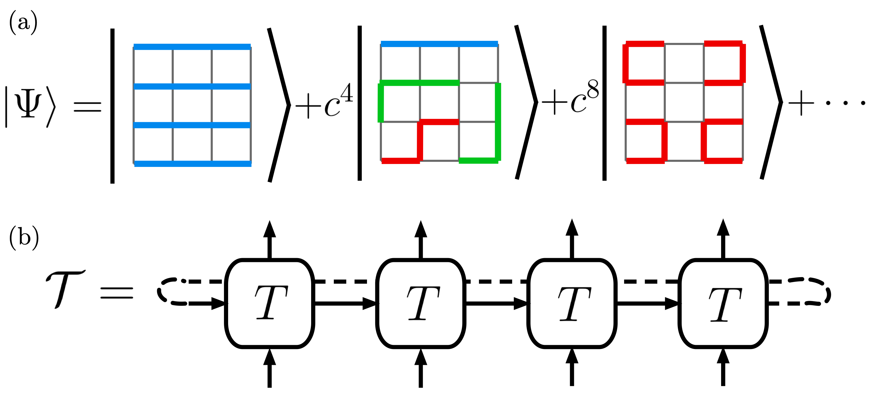
The model: The one-parameter wavefunction we consider is illustrated in Fig. 2(a) for the square lattice. We take a weighted superposition of all tetramer configurations, inspired by a similar construction for the trimer model in Ref. [33]. Up to rotation all possible tetramer shapes we consider are illustrated in Fig. 2(a). The weighting of each tetramer configuration is , where is the total number of bends in that configuration. Thus when only fully bent configurations, i.e. those with only red tetramers, are allowed, while when only fully straight configurations are, i.e. those with only blue tetramers. Explicitly, if is a tetramer configuration then
| (1) |
where
| (2) |
is the weight and is a normalization. Here is the number of fully bent, or red, tetramers in the configuration , likewise with the other colors.
This wavefunction can be represented as a projected entangled pair state (PEPS) on the semi-infinite cylinder using very similar constructions as those in Refs. [39, 33]. Once in PEPS, the correlation length of any operator is controlled by the eigenvalues of the transfer matrix, , one ring of the PEPS contracted with itself [40, 41, 39]. See Fig. 1(e) of Ref. [41] for an illustration of this. For general -mer models it is possible to directly determine the transfer matrix without reference to the PEPS. This was worked out in [39] for generic values of and generic lattices. To build for a generic lattice involves assigning a direction to each bond and placing tensors on each site whose rank is given by the coordination number of that site. For example on the square lattice is rank-, written as and shown in Fig. 2(b). Here is the bottom leg, is the top, the left, and the right with .

The specific form taken by for the wavefunction in Fig. 2(a) is shown in Fig. 3. There is a straightforward way to understand why allows only tetramer configurations by assigning values of on bonds to tetramer links. If any of these values on the bonds is zero, then leave that bond blank, indicating no tetramer. However, if a bond value is nonzero then color the bond red, indicating a tetramer. From Fig. 3 we see immediately that every site must be touched by one, and only one, tetramer. Further inspection shows that when we contract four s on different sites, by pairing equivalent numbers together, only tetramer configurations will survive. The weighting on the left of Fig. 3 assigns a weight of to straight pieces of the tetramer and a weight of to the bent pieces. These appear with a square because the transfer matrix can be thought of as a piece of the wavefunction contracted with itself, naturally leading to squared weights [33].

There is a local symmetry of the tetramer model that the transfer matrix makes clear. Every tetramer shape and orientation can be uniquely broken down into four of the on-site pieces shown in Fig. 3. We can therefore assign numbers taking values in to each of the links of every tetramer (and a value of to every unfilled bond). Further, these numbers obey a local flux conservation. This can be seen by inspection of the vertices in Fig. 3, where there is always a net outgoing flux of . Thus if we draw any path on the dual lattice encircling vertices, then we will enclose flux. In the dimer (trimer) model local () flux conservation leads to () different equivalent sectors on a torus which are distinguished by their winding number [20, 28, 33]. In an exactly analogous way this flux conservation will lead to (at least) different sectors on a torus. However, because we consider a semi-infinite cylinder we expect only a fourfold degeneracy in the spectrum of . Indeed we find numerically that for all values of the logarithm of the largest four eigenvalues of have gaps that close exponentially in , as expected for a transfer matrix with symmetry [41]. We give more detail below.
We note that this local symmetry does not guarantee topological order. For example, in the dimer model on the square lattice the local flux conservation is enlarged to a symmetry, leading to gaplessness and destroying the topological order [20]. Thus the remaining question is whether any of the wavefunctions we consider in Fig. 2(a) can be gapped; if they are then the observation of the symmetry will allow us to conclude the wavefunction realizes the minimal TO.
For the trimer model the question of gaplessness was addressed by Ref. [28] by measuring a variety of correlators at different length scales and concluding that all displayed exponentially decaying behavior, with a correlation length on the order of one to two lattice spacings. However, this left open the possibility that other unmeasured correlators may have power law behavior, indicating gaplessness. This was resolved by Ref. [33] using the fact that at large distances all correlation lengths are upper bounded by
| (3) |
where is the largest eigenvalue of , is the next largest, etc. We do the same for the tetramer model. As mentioned earlier we find a fourfold near degeneracy due to the flux conservation law, so the appropriate ratio to consider is , where the superscript indicates that this is the charge sector of the symmetry. With this caveat in mind we find these eigenvalues numerically using tensor networks. In particular, we treat as a matrix product operator (MPO) and iteratively extract its largest-magnitude eigenvalues and eigenstates using 10 iterations of a DMRG-like Arnoldi method [42]. After obtaining an eigenpair , we update the MPO to (more precisely, only the action of is used), and repeat the procedure to obtain subsequent eigenvalues. In practice, we compute 10 eigenvalues since Arnoldi often returns them slightly out of order. We note that despite the larger bond dimensions of the tetramer model compared to the trimer model we are still able to achieve larger system sizes than considered in [28, 33].
Our results are displayed in Fig. 4. We find that the fully straight tetramer wavefunction displays a diverging correlation length as , indicating gaplessness. The origin of gaplessness can be understood by partitioning the lattice into four sublattices, colored in the inset. Regardless of the orientation a straight trimer can be seen to contain one, and only one, of each color. We can then define three different “electric field” lines that originate from the yellow sublattice and end on the: green, purple, and red sublattices, respectively. The flux of the first field through any region will be given by the number of green sublattice points enclosed minus the number of yellow; likewise for the others. This leads to a flux valued in , giving a local conservation law for each electric field. These conservation laws are independent, as can be seen by arguments nearly identical to those in App. B of Ref. [33]. Thus this state possesses a conservation law, leading to gaplessness [38].
In contrast the fully bent tetramer wavefunction displays a saturating correlation length as . Increasing the bond dimension makes this saturating correlation length clearer. This implies a gapped state which, combined with the degeneracy of , suggests that the fully bent tetramer wavefunction exhibits the minimal TO for a bosonic state at this filling.
We note that we also measured versus for the wavefunction at , i.e. the equal mixture state of all tetramers. There we find an apparently diverging correlation length. However, unlike there is no obvious conservation law leading to gaplessness. This leads us to speculate that this state is gapped, albeit with a very small gap. Thus the saturation of the correlation is not evident at the system sizes we have access to. As , near the fully bent configuration, the gap becomes clear at the system sizes we can access.
Further work: There are a number of possible extensions of this work. First it may be interesting to determine the correlation length in the infinite system limit by the use of tensor network methods such as CTMRG or VUMPS, as in [33]. Additionally we could consider the tetramer model on other lattice geometries. We consider the equal weighted tetramer wavefunction on the triangular lattice in App. A, though we lacked the numerical resources to fully explore that problem. Other lattices, e.g. the kagome lattice, could also be studied.
Studying other lattice geometries may also be helpful to develop more concrete microscopic models for electronic QCLs. In the picture illustrated in Fig. 1(d) each link of the tetramers we consider corresponds to a Cooper pair. The tetramer constraint is very unnatural when viewed from this lens, but may be more natural for tetramers in another lattice geometry. For example, in the trimer case Ref. [33] showed that the all bent trimer wavefunction on the square lattice could be mapped to a boson hopping model on a two layer system. The trimer constraint was then naturally realized as a Rydberg blockade on this lattice. It would be interesting to see if other variants of the tetramer model on other lattice geometries can also have a natural physical realization while maintaining their minimal TO.
Acknowledgements.
S.M. acknowledges helpful discussions with André Grossi Fonseca, Jung Hoon Han, Hosho Katsura, Kyung-Su Kim, T. Senthil, and Victoria Zhang. This work is supported by the Laboratory for Physical Sciences through the Condensed Matter Theory Center.References
- Cheng et al. [2016] M. Cheng, M. Zaletel, M. Barkeshli, A. Vishwanath, and P. Bonderson, “Translational symmetry and microscopic constraints on symmetry-enriched topological phases: A view from the surface,” Physical Review X 6, 041068 (2016).
- Regan et al. [2020] E. C. Regan, D. Wang, C. Jin, M. I. Bakti Utama, B. Gao, X. Wei, S. Zhao, W. Zhao, Z. Zhang, K. Yumigeta, M. Blei, J. D. Carlström, K. Watanabe, T. Taniguchi, S. Tongay, M. Crommie, A. Zettl, and F. Wang, “Mott and generalized Wigner crystal states in WSe2/WS2 moiré superlattices,” Nature 579, 359 (2020).
- Wang et al. [2020] L. Wang, E.-M. Shih, A. Ghiotto, L. Xian, D. A. Rhodes, C. Tan, M. Claassen, D. M. Kennes, Y. Bai, B. Kim, K. Watanabe, T. Taniguchi, X. Zhu, J. Hone, A. Rubio, A. N. Pasupathy, and C. R. Dean, “Correlated electronic phases in twisted bilayer transition metal dichalcogenides,” Nature Materials 19, 861 (2020).
- Xu et al. [2020] Y. Xu, S. Liu, D. A. Rhodes, K. Watanabe, T. Taniguchi, J. Hone, V. Elser, K. F. Mak, and J. Shan, “Correlated insulating states at fractional fillings of moiré superlattices,” Nature 587, 214 (2020).
- Mak and Shan [2022] K. F. Mak and J. Shan, “Semiconductor moiré materials,” Nature Nanotechnology 17, 686 (2022).
- Pan et al. [2020] H. Pan, F. Wu, and S. Das Sarma, “Quantum phase diagram of a Moiré-Hubbard model,” Physical Review B 102, 201104 (2020).
- Pan and Das Sarma [2021] H. Pan and S. Das Sarma, “Interaction-driven filling-induced metal-insulator transitions in 2d Moiré lattices,” Physical Review Letters 127, 096802 (2021).
- Tang et al. [2022] Y. Tang, J. Gu, S. Liu, K. Watanabe, T. Taniguchi, J. C. Hone, K. F. Mak, and J. Shan, “Dielectric catastrophe at the Wigner-Mott transition in a moiré superlattice,” Nature Communications 13, 4271 (2022).
- Kim et al. [2023] S. Kim, T. Senthil, and D. Chowdhury, “Continuous Mott transition in moiré semiconductors: Role of long-wavelength inhomogeneities,” Physical Review Letters 130, 066301 (2023).
- Xu et al. [2022] Y. Xu, X.-C. Wu, M. Ye, Z.-X. Luo, C.-M. Jian, and C. Xu, “Interaction-driven metal-insulator transition with charge fractionalization,” Physical Review X 12, 021067 (2022).
- Musser et al. [2022] S. Musser, T. Senthil, and D. Chowdhury, “Theory of a continuous bandwidth-tuned Wigner-Mott transition,” Physical Review B 106, 155145 (2022).
- Musser and Senthil [2022] S. Musser and T. Senthil, “Metal to Wigner-Mott insulator transition in two-leg ladders,” Physical Review B 106, 235148 (2022).
- Musser et al. [2025] S. Musser, M. Cheng, and T. Senthil, “Fractionalization as an alternate to charge ordering in electronic insulators,” Physical Review B 111, 235108 (2025).
- Krishnan et al. [2025] A. Krishnan, A. Kumar, and T. Senthil, “Defect mediated quantum melting of charge ordered insulators,” (2025), arXiv:2510.00099 [cond-mat].
- Lieb et al. [1961] E. Lieb, T. Schultz, and D. Mattis, “Two soluble models of an antiferromagnetic chain,” Annals of Physics 16, 407 (1961).
- Oshikawa [2000] M. Oshikawa, “Commensurability, excitation gap, and topology in quantum many-particle systems on a periodic lattice,” Physical Review Letters 84, 1535 (2000).
- Hastings [2004] M. B. Hastings, “Lieb-Schultz-Mattis in higher dimensions,” Physical Review B 69, 104431 (2004).
- Rokhsar and Kivelson [1988] D. S. Rokhsar and S. A. Kivelson, “Superconductivity and the quantum hard-core dimer gas,” Physical Review Letters 61, 2376 (1988).
- Ardonne et al. [2004] E. Ardonne, P. Fendley, and E. Fradkin, “Topological order and conformal quantum critical points,” Annals of Physics 310, 493 (2004).
- Moessner and Raman [2008] R. Moessner and K. S. Raman, “Quantum dimer models,” (2008), arXiv:0809.3051 [cond-mat].
- Moessner and Sondhi [2001] R. Moessner and S. L. Sondhi, “Resonating valence bond phase in the triangular lattice quantum dimer model,” Physical Review Letters 86, 1881 (2001).
- Balents et al. [2002] L. Balents, M. P. A. Fisher, and S. M. Girvin, “Fractionalization in an easy-axis Kagome antiferromagnet,” Physical Review B 65, 224412 (2002).
- Senthil and Motrunich [2002] T. Senthil and O. Motrunich, “Microscopic models for fractionalized phases in strongly correlated systems,” Physical Review B 66, 205104 (2002).
- Motrunich and Senthil [2002] O. I. Motrunich and T. Senthil, “Exotic Order in Simple Models of Bosonic Systems,” Physical Review Letters 89, 277004 (2002).
- Ye and Zou [2024] W. Ye and L. Zou, “Classification of Symmetry-Enriched Topological Quantum Spin Liquids,” Physical Review X 14, 021053 (2024).
- Motrunich [2003] O. I. Motrunich, “Bosonic model with fractionalization,” Physical Review B 67, 115108 (2003).
- Myers and Herdman [2017] O. Myers and C. M. Herdman, “ topological order in the quantum dimer-pentamer model,” Physical Review B 96, 174434 (2017).
- Lee et al. [2017] H. Lee, Y.-t. Oh, J. H. Han, and H. Katsura, “Resonating valence bond states with trimer motifs,” Physical Review B 95, 060413 (2017).
- Devakul [2018] T. Devakul, “ topological order in the face-centered-cubic quantum plaquette model,” Physical Review B 97, 155111 (2018).
- Dong et al. [2018] X.-Y. Dong, J.-Y. Chen, and H.-H. Tu, “SU(3) trimer resonating-valence-bond state on the square lattice,” Physical Review B 98, 205117 (2018).
- Kurečić et al. [2019] I. Kurečić, L. Vanderstraeten, and N. Schuch, “Gapped SU(3) spin liquid with topological order,” Physical Review B 99, 045116 (2019).
- Jandura et al. [2020] S. Jandura, M. Iqbal, and N. Schuch, “Quantum trimer models and topological SU(3) spin liquids on the kagome lattice,” Physical Review Research 2, 033382 (2020).
- Giudice et al. [2022] G. Giudice, F. M. Surace, H. Pichler, and G. Giudici, “Trimer states with topological order in Rydberg atom arrays,” Physical Review B 106, 195155 (2022).
- Mao et al. [2023] D. Mao, K. Zhang, and E.-A. Kim, “Fractionalization in fractional correlated insulating states at filled twisted bilayer graphene,” Physical Review Letters 131, 106801 (2023).
- Chen et al. [2025] H. Chen, D. Mao, A. K. Dagnino, G. Wagner, M. H. Fischer, J. Hasik, E.-A. Kim, and T. Neupert, “How quantum fluctuations freeze a classical liquid and then melt it into a topological one,” (2025), arXiv:2504.08895 [cond-mat].
- Han and Kivelson [2023] Z. Han and S. A. Kivelson, “Resonating Valence Bond States in an Electron-Phonon System,” Physical Review Letters 130, 186404 (2023).
- Cai et al. [2024] X. Cai, Z. Han, Z.-X. Li, S. A. Kivelson, and H. Yao, “Quantum spin liquid from electron-phonon coupling,” (2024), arXiv:2408.04002 [cond-mat].
- Polyakov [1977] A. Polyakov, “Quark confinement and topology of gauge theories,” Nuclear Physics B 120, 429 (1977).
- Jandura [2019] S. Jandura, Topological Order in Quantum N-mer Models, Ph.D. thesis, LMU München (2019).
- Cirac et al. [2011] J. I. Cirac, D. Poilblanc, N. Schuch, and F. Verstraete, “Entanglement spectrum and boundary theories with projected entangled-pair states,” Physical Review B 83, 245134 (2011).
- Schuch et al. [2013] N. Schuch, D. Poilblanc, J. I. Cirac, and D. Pérez-García, “Topological Order in the Projected Entangled-Pair States Formalism: Transfer Operator and Boundary Hamiltonians,” Physical Review Letters 111, 090501 (2013).
- Arnoldi [1951] W. E. Arnoldi, “The principle of minimized iterations in the solution of the matrix eigenvalue problem,” Quarterly of Applied Mathematics 9, 17 (1951).
Appendix A Tetramers on the triangular lattice
As in the main text we can map the tetramer wavefunction on the triangular lattice to a transfer matrix. We follow Eq. (3) of [39] to directly construct the transfer matrix. This is now a rank- tensor, , since the triangular lattice has coordination number six. As in Fig. 3 for the square lattice only some configurations of give nonzero values of . In total there are now configurations that give a nonzero value, so we do not plot them all here, but refer interested readers to Eq. (3) of [39]. We considered an equal weight superposition of all tetramer configurations, so we took any nonzero value of to be one rather than weighting by a factor related to the bending of a tetramer.
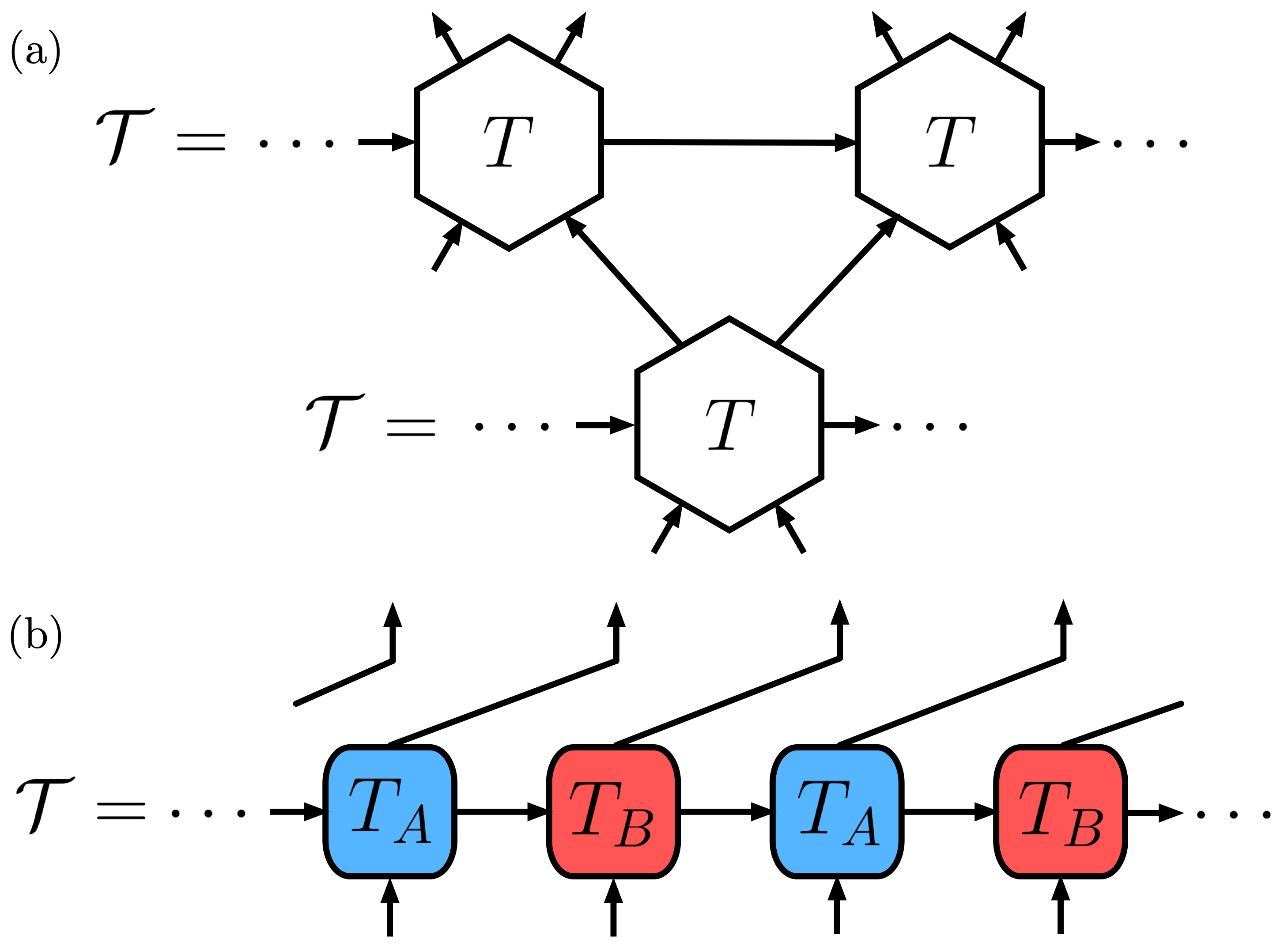
The rank- tensors can be contracted along the legs labeled by Greek characters to form the transfer matrix, . We have plotted a segment of this in Fig. 5(a). Importantly the triangular case requires a shift by half a lattice site when stacking . This proves challenging to diagonalize, so instead we decompose into two rank- tensors and using a SVD decomposition. We are thus able to return our transfer matrix to the square lattice form, with this additional lattice shift. However, this transformation reveals the extra costs of diagonalizing on the triangular lattice. It effectively doubles the number of lattice sites for a given cylinder circumference , and also increases the bond dimension on the virtual legs.
Despite both of these challenges, the difficulty arises primarily because the MPO is not composed of a single , but of two layers. These MPOs cannot be freely stacked because of the geometry of the triangular lattice. Instead, for the first layer, the first site must be moved to the end through repeated swap operations, while for the second layer the reverse must be done, in order to construct a total MPO with periodic boundaries on the sites that can then be stacked. These repeated long-range swap operations substantially increase the bond dimension of the total MPO and scale very poorly with system size. For example, the MPO for a lattice had a bond dimension of . Combined with the fact that the effective chain length is doubled, this makes the case comparable to solving a 40-site four-level chain with a very large-MPO bond dimension. In addition, when iteratively targeting higher excited eigenvalues, one must include the outer product of each previously obtained eigenstate, which further increases the computational cost. Because the MPS itself already has a moderate bond dimension, this process further enlarges the effective MPO at each eigenvalue iteration. In practice, the full MPS-MPO composite MPO is not constructed explicitly, but its action still carries a substantial computational cost. At an MPS bond dimension of 400, computing the largest 10 eigenstates required roughly 20 days for a cylinder circumference of , making larger system sizes prohibitively expensive.

Despite the numerical difficulty of finding the largest eigenvalues of on the triangular lattice we were able to determine the upper bound on the correlation length for small cylinder circumferences and small bond dimensions. The results are shown in Fig. 6. While they appear consistent with a saturating correlation length as , and thus with a gapped TO, it is difficult to say anything precise given the disagreement between different bond dimensions at . Further it is not feasible for us to attempt larger values of or , as doing so would take several months to a year on our current hardware. As such we have left this problem for future work.