¹¹institutetext: Astronomical Observatory, University of Warsaw, Al. Ujazdowskie 4, 00-478 Warsaw, Poland.

Recovering cosmological parameters from the mock
gravitational wave data of the Einstein Telescope

Pinaki Roy ^, Tomasz Bulik

(Received MMMMM DD, YYYY; accepted MMMMM DD, YYYY)

Context. Einstein Telescope (ET) is a third-generation gravitational wave (GW) detector with tenfold better sensitivity compared to the advanced LIGO detectors. It will be capable of observing copious stellar mass binary black hole mergers upto a redshift of 10 which will make it especially useful for cosmography.
Aim. We generate a mock gravitational wave event catalog for the Einstein Telescope and show the recoverability of either the Hubble constant ( $H_{0}$ ) or the matter density parameter ( $\Omega_{\rm m}$ ).
Methods. We present a simple, effective and fast technique for inferring $H_{0}$ (or $\Omega_{\rm m}$ ) using the intrinsic chirp mass spectrum of black hole binaries, and investigate the efficacy of the method assuming the standard model of cosmology.
Results. If only $H_{0}$ has to be constrained, we find that at least one year of ET’s observation will be required to achieve 1% uncertainty. With the same amount of observation, $\Omega_{\rm m}$ can be constrained to within 4% uncertainty.
Conclusion. With ET operating as a standalone instrument, we show that the GW spectral sirens detected by it can constrain the Hubble constant.

Key Words.:

Gravitational waves; Stars: neutron, black holes; Methods: data analysis

1 Introduction

The advent of gravitational wave (GW) astronomy with second-generation detectors like LIGO and Virgo has unveiled a population of merging compact binaries and provided groundbreaking multi-messenger insights. The future Einstein Telescope (ET), a third-generation GW telescope (Punturo et al. 2010), promises a quantum leap in sensitivity. The annual detection rates based on the sensitivity for ET’s triangular design (Hild et al. 2011), namely ET-D, are expected to be $\sim 10^{5}-10^{6}$ binary black hole mergers (roughly 1 event every 100 seconds) and $\sim 7\times 10^{4}$ binary neutron star mergers (roughly 2 events every 15 minutes) (see Regimbau et al. 2012, 2014; Belgacem et al. 2019). These high detection rates will make ET a powerful tool for population studies as well as cosmography.

A key limitation for a single observatory such as the current GW detectors is the difficulty in localizing sources and breaking degeneracies between the intrinsic chirp mass of the GW source (merging binary) and the source redshift. Singh and Bulik (2021) showed how to address this challenge for the ET-D design by utilizing the antenna response of ET’s three detectors. By analyzing the ratios of signal-to-noise and phase differences between the detectors, one can constrain the sky location, inclination, and polarization of the source. This, in turn, allows us to infer the luminosity distance of the source. From this, one can estimate the source redshift by assuming a cosmological model. However, if the cosmology to be used is uncertain, one can avail the vast catalog of GW events detected by ET to eliminate this uncertainty.

To break the degeneracy between the source redshift and the intrinsic chirp mass of the binary, one can obviously exploit any associated electromagnetic (EM) transient to constrain the sky position with high accuracy Schutz (1986); Abbott et al. (2017), subsequently identify the host galaxy and get the redshift distance. Such events are called bright sirens. GW events without an EM counterpart are referred as dark sirens. In such scenarios, one has to resort to statistical techniques to lift the degeneracy. The most popular of these is the galaxy survey method in which one cross-correlates the sky localization volume with galaxy catalogs in order to identify potential host galaxies (see, e.g. Del Pozzo 2012; Chen et al. 2018; Fishbach et al. 2019; Gair et al. 2023) and thus, get the probable redshift values of the source.

A novel way is the spectral siren method, which exploits features in the source-frame mass distribution (also called the mass spectrum) of the merging binary systems, and use a large catalog of events to statistically break the mass-redshift degeneracy (see, e.g. Taylor et al. 2012; Farr et al. 2019; You et al. 2021; Mastrogiovanni et al. 2021). This approach facilitates an independent inference of cosmological parameters. The features in the mass spectrum arise from various parameters governing the binary evolution process (see Tauris and van den Heuvel 2023).

We aim to leverage the intrinsic chirp mass distribution of binary black hole systems and ET’s detection and localization capability to infer the Hubble constant and the matter density parameter. Our work differs from similar recent studies (see, e.g. Ezquiaga and Holz 2022; Roy et al. 2025; Califano et al. 2025; Tagliazucchi et al. 2026). We include low-SNR and high-redshift events in the mock data. We do not distinguish between NS-BH and BH-BH binaries in our analysis. To the best of our knowledge, the KL divergence method we adopt has not been applied to this cosmography with spectral siren problem so far. Our approach can also be applied to the full mass spectrum but we reserve that exercise for a future study.

This paper is organized as follows. In Section 2, we lay out the steps to build the mock GW data for ET. In Section 3, we present our results obtained with the mock data. In Section 4, we list the takeaways from our study and future plans.

2 Method

We first describe the scheme for creating the mock data catalog for ET followed by a description of how we use the event catalog for cosmography. We have assumed standard model of cosmology (SMOC) throughout the analysis. In the minimal 6-parameter $\Lambda$ CDM model, the curvature density parameter, $\Omega_{k}=0$ , the radiation density parameter, $\Omega_{\rm rad}=0$ and the dark energy equation of state parameter, $w=-1$ . Then, the matter density parameter ( $\Omega_{\rm m}$ ) and the dark energy density parameter ( $\Omega_{\Lambda}$ ) sum to unity, i.e. $\Omega_{\text{m}}+\Omega_{\Lambda}=1$ .

In this work, we first set ourselves the goal of recovering $H_{0}$ for two cases with different injected $H_{0}$ values. The two values lie at the typical extremes of the measured range of values. For Case I, we have used 67.3 km s^-1 Mpc^-1, whereas for Case II, we have used 73.5 km s^-1 Mpc^-1. In both these cases, we have set $\Omega_{\rm m}=0.3$ . Then, we aim to recover $\Omega_{\rm m}$ keeping $H_{0}$ fixed at 70 km s^-1 Mpc^-1. For this, we prepare two more cases viz. Case III: $\Omega_{\rm m}=0.27$ and Case IV: $\Omega_{\rm m}=0.32$ . Further, we consider additional cases with the injected values: $H_{0}=70$ km s^-1 Mpc^-1 and $\Omega_{\rm m}=0.3$ , assuming some systematic uncertainty in the fixed parameter.

We generate compact binary population using the publicly available binary population synthesis code COMPAS (Riley et al. 2022) v03.07.02 which can rapidly evolve isolated binaries through all the important stages of evolution such as the Roche lobe overflow (RLOF), mass transfer, supernova and common envelope. We evolve 1 million zero-age main sequence (ZAMS) binaries with Kroupa mass function and thermal eccentricity distribution for each of the 76 different metallicity values: $Z=0.0001-0.0020$ (in steps of 0.0001), $Z=0.0025-0.0300$ (in steps of 0.0005).

As in COMPAS, so do we, in our analysis, identify a compact object as a neutron star if it is below 2.5 $M_{\odot}$ and as a black hole if it is above this mass limit. We choose the minimum initial ZAMS mass as 5 $M_{\odot}$ . The and maximum initial mass is the kept to its default value of 150 $M_{\odot}$ . Later, we correct the compact binary yield by multiplying it with the correction factor 0.019.

The redshift-dependent formation efficiency information for the different kinds of compact binaries, viz. NS-NS, NS-BH and BH-BH, together with a metallicity-dependent star formation rate model, is then used to determine the concentration of compact binaries merging at various redshifts following the method described by Mapelli et al. (2017). We have used a metallicity-independent binary fraction of 0.5 and a redshift limit of $\sim$ 10. Binary fraction is defined as $f_{\rm b}=n_{\rm b}/(n_{\rm s}+n_{\rm b})$ where $n_{\rm b}$ and $n_{\rm s}$ are the number of binary and the number of single star systems, respectively. Thus, a binary fraction of 0.5 implies that one-third of the stars in the ensemble are single whereas two-third of the stars are in binaries.

We chose for our mock data synthesis the model which gave a local merger rate density consistent with the constraint reported in Abbott et al. (2023). We adopt an observationally motivated metallicity-dependent star formation rate (SFR), specifically, the model 206f14SBBoco_FMR170 from Chruślińska et al. (2021) which resembles the Madau-Dickinson SFR (Madau and Dickinson 2014) when summed over metallicities. However, we assert that adopting a perfect binary evolution model or the best metallicity-dependent star formation rate model is not necessary for the problem at hand. The goal is to use an adequately broad intrinsic chirp mass spectrum as an anchor to lift the mass-redshift degeneracy for GW events.

2.1 Mock event catalog: Detectability

The strain (amplitude), $h$ , in the interferometer arm of length, $l$ , of a GW detector is given by (see, for e.g. Allen et al. 2012)

\displaystyle h(t)

\displaystyle=-\left(\dfrac{G\mathcal{M}_{z}}{c^{2}d_{L}}\right)\left(\dfrac{t_{c}-t}{5G\mathcal{M}_{z}/c^{3}}\right)^{-1/4}\left(\dfrac{\Theta}{4}\right)\cos{(2\Phi_{0}+2\Phi_{\rm N})}

(1)

where $\mathcal{M}=(m_{1}m_{2})^{3/5}/(m_{1}+m_{2})^{1/5}$ is the chirp mass of the binary, and $\mathcal{M}_{z}=(1+z)\mathcal{M}$ is the redshifted chirp mass. $t_{c}$ and $\Phi_{c}$ are time and phase of the binary coalescence i.e. $\Phi(t=t_{c})=\Phi_{c}$ . $\Phi_{0}=\Phi_{c}+\Phi_{0}^{\prime}$ is the termination phase of the GW signal, and

	$\displaystyle\Phi_{\rm N}$	$\displaystyle=-\left(\dfrac{t_{c}-t}{5G\mathcal{M}_{z}/c^{3}}\right)^{5/8}$		(2)
	$\displaystyle\Phi_{0}^{\prime}$	$\displaystyle=-\dfrac{1}{2}\tan^{-1}{\dfrac{2F_{\times}\cos{\iota}}{F_{+}(1+\cos^{2}{\iota})}}$		(3)

where $\iota$ is the orbital inclination of the binary to the line of sight. $\Theta$ is the orientation function of the detector. For the $i$ -th detector,

\displaystyle\Theta_{i}=4\left[F_{+,i}^{2}\left(\dfrac{1+\cos^{2}{\iota}}{2}\right)^{2}+F_{\times,i}^{2}\cos^{2}{\iota}\right]^{1/2}

(4)

such that $0<\Theta_{i}<4$ . $F_{+,i}$ and $F_{\times,i}$ are the antenna pattern functions of the $i$ -th interferometer for the $+$ and $\times$ polarizations of the incoming GW signal which are expressed as (see, e.g. Sathyaprakash and Schutz 2009):

	$\displaystyle F_{+,1}=\sin\gamma\left[\dfrac{1}{2}(1+\cos^{2}\theta)\cos 2\phi\cos 2\psi-\cos\theta\sin 2\phi\sin 2\psi\right]$		(5)
	$\displaystyle F_{\times,1}=\sin\gamma\left[\dfrac{1}{2}(1+\cos^{2}\theta)\cos 2\phi\sin 2\psi+\cos\theta\sin 2\phi\cos 2\psi\right]$		(6)

where $\phi$ and $\theta$ are, respectively, the azimuthal and polar angles of the source location in the sky. $\psi$ is the GW polarization angle.

These response functions are smaller by a factor of $\sin\gamma=\sqrt{3}/2$ ( $\gamma=\pi/3$ for ET-D) compared to those of an L-shaped interferometer with the same arm length. The response functions of the other two interferometers in ET, with arms are obtained from $F_{+,1}$ and $F_{\times,1}$ by the transformation $\phi\to\phi\pm 2\pi/3$ .

	$\displaystyle F_{+,\times,2}(\theta,\phi,\psi)=F_{+,\times}^{(1)}(\theta,\phi+2\pi/3,\psi)$		(7)
	$\displaystyle F_{+,\times,3}(\theta,\phi,\psi)=F_{+,\times}^{(1)}(\theta,\phi-2\pi/3,\psi)$		(8)

It can be showed that

	$\displaystyle F_{+,1}^{2}+F_{+,2}^{2}+F_{+,3}^{2}\Big\|_{\rm max}=3\sin^{2}\gamma/2=9/8$		(9)
	$\displaystyle F_{\times,1}^{2}+F_{\times,2}^{2}+F_{\times,3}^{2}\Big\|_{\rm max}=3\sin^{2}\gamma/2=9/8$		(10)

Once the redshift distribution of the synthetic compact binary merger population is accomplished, the binaries are then distributed isotropically across the sky and assigned the four angles: ( $\phi,\theta,\iota,\psi$ ). Thereafter, they are checked for detectability using ET’s design sensitivity, $S_{h}(f)$ . For this, we calculate the signal-to-noise ratios (SNRs) in ET’s three interferometers denoted by $i=1,2,3$ .

\displaystyle\rho_{i}=2\,\sqrt{\dfrac{5}{24}}\,\left(\dfrac{\Theta_{i}}{4}\right)\dfrac{(G\mathcal{M}_{z})^{5/6}}{\pi^{2/3}c^{3/2}d_{L}}\sqrt{\displaystyle\int_{1}^{2f_{\rm max}}\dfrac{df}{f^{7/3}S_{h}(f)}}

(11)

(see Finn 1996; Taylor and Gair 2012) where $d_{L}$ is the luminosity distance of the source, $f$ is the GW frequency, and $2f_{\rm max}$ is the peak GW frequency given by (see, e.g. Taylor et al. 2012)

\displaystyle 2f_{\rm max}=\dfrac{c^{3}}{6\sqrt{6}\pi GM}\approx\dfrac{4400\ \text{Hz}}{1+z}\left(\dfrac{M_{\odot}}{M}\right)

(12)

The effective SNR, $\rho_{\rm eff}$ , is defined as $\rho_{\rm eff}=\sqrt{\rho_{1}^{2}+\rho_{2}^{2}+\rho_{3}^{2}}$

Once the three SNRs for an event are computed, the event is classified as detected or undetected based on the condition: $\rho_{i}\geq 2$ and $\rho_{\rm eff}\geq 5$ . This lower threshold condition (compared to the commonly used $\rho_{i}\geq 3$ and $\rho_{\rm eff}\geq 8$ ) is chosen to increase the number of detected events which is necessary for cosmography.

2.2 Mock event catalog: Observables

Once the detectable events are identified, we proceed to determine the observables, $\mathcal{M}_{z}$ and $d_{L}$ , from the SNRs and phases of the GW signal.

The redshifted chirp mass, $\mathcal{M}_{z}$ , can be derived from the GW frequency and its time derivative as

\displaystyle\mathcal{M}_{z}=\dfrac{c^{3}}{G}\left(\dfrac{5}{96\pi^{8/3}}\dfrac{\dot{f}_{\rm GW}}{f_{\rm GW}^{11/3}}\right)^{3/5}

(13)

where $\dot{f}_{\rm GW}=df_{\rm GW}/dt$ . We assume ${\mathcal{M}_{z}}$ to be the same as the injected value, albeit, with a Gaussian error of $\mathcal{M}_{z}/\rho_{\rm eff}$ (see Singh and Bulik 2021). Thus, we get $P({\mathcal{M}_{z}})$ for all the events.

Furthermore, we assume that the measurement error on each of the three SNRs is $\sigma_{\rho}=1$ , and on each of the three phases is $\sigma_{\Phi}=\pi/\rho$ . We obtain the SNR ratios: $\rho_{21}=\rho_{2}/\rho_{1}$ and $\rho_{31}=\rho_{3}/\rho_{1}$ and the phase differences: $\Phi_{21}=\Phi_{0,2}-\Phi_{0,1}$ and $\Phi_{31}=\Phi_{3,0}-\Phi_{0,1}$ . The probability density of the SNR ratios and the phase differences are given by

	$\displaystyle P(\rho_{j1})=$	$\displaystyle\displaystyle\int d\rho_{1}\displaystyle\int d\rho_{j}\,P(\rho_{1})\,P(\rho_{j})\,\,\delta\big(\rho_{j1}-(\rho_{j}/\rho_{1})\big)$		(14)
	$\displaystyle P(\Phi_{j1})=$	$\displaystyle\displaystyle\int d\Phi_{1}\displaystyle\int d\Phi_{j}\,P(\Phi_{1})\,P(\Phi_{j})\,\delta\big(\Phi_{j1}-(\Phi_{j}-\Phi_{1})\big)$		(15)

respectively, where $j=2,3$ .

\displaystyle P(\rho_{\rm eff})=\displaystyle\int d\rho_{1}\displaystyle\int d\rho_{2}\displaystyle\int d\rho_{3}\,P(\rho_{1})\,P(\rho_{2})\,P(\rho_{3})\,\delta\big(\rho_{\rm eff}-\rho_{0}\big)

(16)

where $\rho_{0}=\sqrt{\rho_{1}^{2}+\rho_{2}^{2}+\rho_{3}^{2}}$ is the measured $\rho_{\rm eff}$ .

For convenience, one can use propagation of errors to obtain

	$\displaystyle\sigma(\rho_{j1})$	$\displaystyle=\rho_{j1}\sqrt{(1/\rho_{j})^{2}+(1/\rho_{1})^{2}}$		(17)
	$\displaystyle\sigma(\Phi_{j1})$	$\displaystyle=\pi\sqrt{(1/\rho_{j})^{2}+(1/\rho_{1})^{2}}$		(18)

\displaystyle\sigma(\rho_{\rm eff})

\displaystyle=1

(19)

and approximate $P(\rho_{21}),P(\rho_{31}),P(\Phi_{21}),(\Phi_{31})$ and $P(\rho_{\rm eff})$ as Gaussians in which case Equations 14–16 are obsolete.

Following Singh and Bulik (2021), we outline here the steps to recover the source position in the sky.

Let $D_{1}\equiv(\rho_{21},\rho_{31},\Phi_{21},\Phi_{31})$ , $\Omega_{\rm sky}\equiv(\phi,\theta)$ and $\Omega_{\rm source}\equiv(\iota,\psi)$ for a given GW event. Then, using the Bayes’ theorem,

\displaystyle P(\Omega_{\rm sky},\Omega_{\rm source}|D_{1},I)=\dfrac{P(\Omega_{\rm sky},\Omega_{\rm source}|I)P(D_{1}|\Omega_{\rm sky},\Omega_{\rm source},I)}{P(D_{1}|I)}

(20)

As the prior probability $P(\Omega_{\rm sky},\Omega_{\rm source}|I)$ is uniform on both the source and the detector sphere, it becomes:

\displaystyle P(\Omega_{\rm sky},\Omega_{\rm source}|I)=P(\Omega_{\rm eff}|I)=\dfrac{1}{(4\pi)^{2}}

(21)

The likelihood is given by

where

	$\displaystyle\rho_{j1}(\Omega_{\rm sky},\Omega_{\rm source})$	$\displaystyle=\Theta_{j}/\Theta_{1}=\Theta_{j1}(\Omega_{\rm sky},\Omega_{\rm source})$		(23)
	$\displaystyle\Phi_{j1}(\Omega_{\rm sky},\Omega_{\rm source})$	$\displaystyle=\Phi_{0,j}(\Omega_{\rm sky},\Omega_{\rm source})-\Phi_{0,1}(\Omega_{\rm sky},\Omega_{\rm source})$		(24)

The posteriors for $\Omega_{\rm sky}$ and $\Omega_{\rm source}$ then become

	$\displaystyle P(\Omega_{\rm sky}\|D_{1},I)=\displaystyle\int P(\Omega_{\rm sky},\Omega_{\rm source}\|D_{1},I)\,d\Omega_{\rm source}$		(25)
	$\displaystyle P(\Omega_{\rm source}\|D_{1},I)=\displaystyle\int P(\Omega_{\rm sky},\Omega_{\rm source}\|D_{1},I)\,d\Omega_{\rm sky}$		(26)

The effective orientation function is defined as $\Theta_{\rm eff}=\sqrt{\Theta_{1}^{2}+\Theta_{2}^{2}+\Theta_{3}^{2}}$ so that $0<\Theta_{\rm eff}<6$ (using Equations 4-10). Assuming a flat prior on $\Theta_{\rm eff}$ , we have

\displaystyle P(\Theta_{\rm eff}|I)=\dfrac{1}{\Theta_{\rm eff,\,max}}=\dfrac{1}{6}

(27)

\displaystyle P(\Theta_{\rm eff}|D_{1},I)=\displaystyle\int d\Omega_{\rm eff}\,P(\Theta_{\rm eff}|I)\,P(\Omega_{\rm eff}|D_{1},I)\,\delta(\Theta_{\rm eff}-\Theta_{\rm eff}(\Omega_{\rm eff}))

(28)

Substituting Equation 20 in 28 gives the $P(\Theta_{\rm eff}$ ), where the dependence of $\Theta_{\rm eff}$ on the position in the sky, polarization and inclination is explicitly included.

Lastly, the luminosity distance of the event may be obtained from the expression:

\displaystyle P(d_{L})=\displaystyle\int d\rho_{\rm eff}P(\rho_{\rm eff})\displaystyle\int d\Theta_{\rm eff}P(\Theta_{\rm eff})\,\delta(d_{L}-d_{L}(\rho_{\rm eff},\Theta_{\rm eff}))

(29)

where $P(\Theta_{\rm eff})=P(\Theta_{\rm eff}|D_{1},I)$ , and the luminosity distance,

\displaystyle d_{L}(\rho_{\rm eff},\Theta_{\rm eff})=2\,\sqrt{\dfrac{5}{24}}\,\left(\dfrac{\Theta_{\rm eff}}{4}\right)\dfrac{(G\mathcal{M}_{z})^{5/6}}{\pi^{2/3}c^{3/2}\rho_{\rm eff}}\sqrt{\displaystyle\int_{1}^{2f_{\rm max}}\dfrac{df}{f^{7/3}S_{h}(f)}}

(30)

This is termed as the recovered luminosity distance. The set of $P(d_{L})$ and $P(\mathcal{M}_{z})$ pairs constitute the mock GW event catalog. Although impractical, we remove all the NS-NS merger events from the catalog to keep the analysis brief.

2.3 Cosmography

In the minimal SMOC, the luminosity distance depends on the redshift as

\displaystyle d_{L}(z,H_{0})=\dfrac{c}{H_{0}}(1+z)\displaystyle\int_{0}^{z}\dfrac{dz^{\prime}}{\sqrt{\Omega_{\rm m}(1+z^{\prime})^{3}+(1-\Omega_{\rm m})}}

(31)

The above equation can be numerically inverted to obtain $z(d_{L},H_{0})$ .

In order to do cosmological inference with a broad intrinsic mass spectrum and low SNR-inclusive event catalog, we shall use all the $N$ detected events together in a Monte Carlo fashion. In a given iteration $i$ , for every event, we pick a $d_{L}$ value and an $\mathcal{M}_{z}$ value based on its $P(d_{L})$ and $P(\mathcal{M}_{z})$ . For a certain event $k$ ( $k\in[1,N]$ ), let us call them $d_{L,\,ik}$ and $\mathcal{M}_{z,\,ik}$ . We start with a certain prior of $H_{0}$ , which, in our case, is 60–80 km s^-1 Mpc^-1. We divide this range into $J$ equispaced $H_{0}$ values. In our simulation, we use $J=200$ . The narrow prior for $H_{0}$ has been used to reduce the computation time. One may use a wider prior for $H_{0}$ as well and the results will be similar. For each $H_{0}$ value (indexed by $j$ ), we find the corresponding $z_{ijk}$ value using $z_{ijk}=z(d_{L,ik},H_{0,j})$ , and then the $\mathcal{M}_{ijk}$ value using $\mathcal{M}_{ijk}=\mathcal{M}_{z,ik}/(1+z_{ijk})$ .

Refer to caption — Figure 1: Intrinsic chirp mass distribution of the merging NS-BH and BH-BH systems. The chirp mass range of the injected sources is 1.6–40 $M_{\odot}$ .

We then collect the $\mathcal{M}_{ijk}$ for all the events and obtain the probability distribution, $P_{ij}(\mathcal{M})$ , and compare it with the model (expected) intrinsic distribution, $P(\mathcal{M})$ (Figure 1), by finding the Kullback–Leibler (KL) divergence, $D_{\text{KL},ij}\left(P(\mathcal{M})\parallel P_{ij}(\mathcal{M})\right)$ .

\displaystyle P_{ij}(\mathcal{M})\approx\sum_{l}{C_{l}\,\text{rect}\left(\dfrac{\mathcal{M}_{ijk}-\mathcal{M}_{l}}{W}\right)}

(32)

where $C_{l}$ is the count in the $l$ -th chirp mass bin, and $W$ is the binwidth. The chirp mass distribution is divided into 100 bins, so $l\in[1,100]$ . “rect” refers to the rectangle function defined by

\displaystyle\text{rect}\,(x)=\begin{cases}1,&|x|\leq 1/2\\ 0,&\text{otherwise}\end{cases}

(33)

It is important to use a chirp mass range much broader than the intrinsic chirp mass range in order to account for the errors on $d_{L}$ and $\mathcal{M}_{z}$ which may yield $\mathcal{M}_{ijk}$ outside the intrinsic chirp mass range. We use the chirp mass range $[0.1,150]\,M_{\odot}$ .

If $P$ is the true probability distribution and $Q$ is an approximating probability distribution, the KL divergence (Kullback and Leibler 1951), also known as relative entropy, is defined as

\displaystyle D_{\text{KL}}(P\parallel Q)=\sum_{x\in\mathcal{X}}P(x)\ln\dfrac{P(x)}{Q(x)}

(34)

where $\mathcal{X}$ is the set of bins into which both the distributions are divided, say 100. $P(x)$ and $Q(x)$ are the probability density values at $x$ . We use KL divergence against other divergences because it is directional and asymmetric as evident from its definition.

Out of the $J$ $D_{\text{KL},ij}$ values, the best $H_{0}$ for the $i$ -th iteration is the one for which $D_{\text{KL},ij}$ is minimum (see Figure 2).

\displaystyle H_{0,i}=H_{0,j}:D_{\text{KL},i}=\text{min}_{j}(D_{\text{KL},ij})

(35)

We perform $n=10000$ such iterations and create a histogram of the $H_{0}$ values. From the kernel density estimate of the $H_{0}$ data, we derive the global best $H_{0}$ . Therefore, we may express the probability distribution as

\displaystyle\hat{P}(H_{0})=\dfrac{1}{nh}\sum_{i=1}^{n}K\left(\dfrac{H_{0}-H_{0,i}}{h}\right)

(36)

(see Hastie et al. 2001) where the bandwidth, $h=n^{-0.2}\approx 0.16$ by Scott’s rule (Scott 1992). $K(x)$ is a Kernel function.

For the Gaussian kernel, the above equation becomes

\displaystyle\hat{P}(H_{0})=\dfrac{1}{n}\sum_{i=1}^{n}\dfrac{1}{(h\sigma)\sqrt{2\pi}}\exp{\left(\dfrac{-(H_{0}-H_{0,i})^{2}}{2(h\sigma)^{2}}\right)}

(37)

where $\sigma$ is the sample standard deviation.

Next, we carry out a similar analysis to recover $\Omega_{\rm m}$ , the prior for which is chosen to be 0.2–0.4.

3 Results

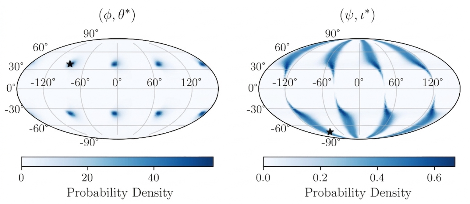
Once an event in the set of injected GW events is classified as detected based on the SNR threshold, it is taken up for localization and subsequently, distance estimation. An example of source localization is shown in Figure 3. The multiple zones in the maps are due to the various angular symmetries in the Equations 5–8. Following Equations 29–31, one gets the probable distance i.e. $P(d_{L})$ of the source whose accuracy depends both on the effective SNR and the SNR ratios (see Figure 4). The higher the effective SNR and the farther the SNR ratios from unity, the better the recovery of the source position. While the effective SNR is primarily effected by the chirp mass and the source distance, the SNR ratios are effected by the coordinates of the source.

The SNR asymmetry, $Y(\rho)$ , may be defined as

\displaystyle Y(\rho)=\text{max}(\rho_{j}/\rho_{i},\rho_{i}/\rho_{j})-1

(38)

where $i,j\in[1,2,3]$ and $i\neq j$ . The $\max$ function ensures that the ratio is greater than unity. For perfect symmetry i.e. $\rho_{1}=\rho_{2}=\rho_{3}$ , $Y(\rho)=0$ .

We prepare six mock datasets. Each dataset consists of the detected BH-BH and BH-NS events from the $10^{5}$ injected binary merger events in some standard cosmological model characterized by $H_{0}$ and $\Omega_{\rm m}$ . With the detection criteria as $\rho_{\rm eff}\geq 5$ , we detect around 55000 BH-NS and BH-BH events in all datasets, leaving out the NS-NS events for simplicity. In every dataset, around 5/6-th of the injected BH-BH and BH-NS events are detected with ${\rm SNR}\geq 5$ . The plot of recovered $d_{L}$ versus injected $d_{L}$ for one of the datasets is shown in Figure 5. The injected values of the ( $H_{0},\Omega_{m}$ ) pair for each case are detailed in Table 1.

We use the binary BH intrinsic chirp mass spectrum derived from simulation. In the first case, with 54850 detected mock BH-BH and BH-NS events, we recover an $H_{0}$ value of $67.8_{-2.2}^{+2.6}$ km s^-1 Mpc^-1 when the injected value is $67.3$ km s^-1 Mpc^-1. Whereas, in the second case, with 56455 detected events, we get an $H_{0}$ value of $73.3_{-2.2}^{+3.2}$ km s^-1 Mpc^-1 when the injected value is $73.5$ km s^-1 Mpc^-1 (see Figure 6). The quoted errors correspond to the 90% credible interval. Thus, with $\sim\,5\times 10^{4}$ events, the statistical uncertainty in the inferred $H_{0}$ is around 3.5%. Cases I and II show that the recovered $H_{0}$ tracks the injected $H_{0}$ .

It may be noted that $\sim$ 90% of the detected mergers originate from $d_{L}<$ 40 Gpc i.e. $z<\,\sim 4$ (see Figure 7). So, mergers from higher redshifts do not have significant contribution to the $H_{0}$ or the $\Omega_{\rm m}$ estimate.

We then proceed to infer $\Omega_{\rm m}$ keeping $H_{0}$ fixed for two cosmological cases, III and IV. With 55105 detected binary BH events, for case III, we recover an $\Omega_{\rm m}$ value of $0.262_{-0.042}^{+0.032}$ against an injected value of 0.27. For case IV, we recover an $\Omega_{\rm m}$ value of $0.310_{-0.042}^{+0.043}$ against an injected value of 0.32 with 55767 events (see Figure 8). Cases III and IV show that the recovered $\Omega_{\rm m}$ tracks the injected $\Omega_{\rm m}$ .

Cases V and VI are similar to case I / II and case III / IV, respectively, but with new datasets. Next, we consider six cases wherein a systematic Gaussian uncertainty is assumed in the value of the known parameter. Lastly, we take up two cases, XIII and XIV, wherein the known parameter is specified to lie in a small range with a uniform distribution. For each of these eight cases, we use three datasets of which the third one is the combination of the other two datasets. The third dataset was used to see if the statistical uncertainty in the parameter estimation drops in the same manner (i.e. by $1/\sqrt{N}$ ) as in the cases V and VI where the known parameter has no systematic uncertainty. All these ten cases have been explored with mock datasets 5 and 6 both of which concern the cosmological model: $[H_{0},\Omega_{\rm m}]=[70,0.3]$ .

For cases VII, IX and XI, we assume that $\Omega_{\rm m}$ is known with an uncertainty of 3%, 6% and 9%, respectively. This results in 3.1%, 3.8% and 5% uncertainties in the $H_{0}$ estimate with 111009 events. With roughly half the number of events, the uncertainties are $\sim$ 3.9%, $\sim$ 4.5% and $\sim$ 5.4%, respectively. For cases VIII, X and XII, we assume that $H_{0}$ is known with an uncertainty of 1%, 2% and 3%, respectively. This results in 12.2%, 15.2% and 20.9% uncertainties in the $\Omega_{\rm m}$ estimate with 111009 events. With roughly half the number of events, the uncertainties are $\sim$ 14.5%, $\sim$ 18.3% and $\sim$ 24.9%, respectively. Thus, the decline in the statistical uncertainty deviates from the $1/\sqrt{N}$ rule as the systematic uncertainty in the known parameter increases.

In case XIII, we assume that $\Omega_{\rm m}$ can be anywhere in the range $[0.25,0.35]$ with a uniform probability. Using 111009 events, we recover an $H_{0}$ value of $69.6_{-2.7}^{+4.5}$ km s^-1 Mpc^-1 (see Figure 9) and the uncertainty is 5.2%. Likewise, in case XIV, we assume that $H_{0}$ can be anywhere in the range $[65,75]$ km s^-1 Mpc^-1 with a uniform probability. Using 111009 events, we recover an $\Omega_{\rm m}$ value of $0.250_{-0.038}^{+0.121}$ (see Figure 9) and the uncertainty is 31.8%. Compared to when only about half of the events are considered, the relative decline in the uncertainty is only $\sim$ 10% for cases XIII and XIV.

The results have been summarized in Table 1. The results for dataset 5+6 are obtained from separate runs, not by combining the results for datasets 5 and 6.

In the presence of a systematic uncertainty on the known parameter, the net uncertainty takes the form:

\displaystyle\varsigma_{\rm net}=\sqrt{\varsigma_{\rm stat,0}^{2}/\lambda+\kappa^{2}\varsigma_{\rm sys}^{2}}

(39)

where $\varsigma$ denotes the relative uncertainty with $N$ events, $\varsigma_{\rm stat,0}$ is the net uncertainty with $N_{0}$ events when the systematic uncertainty is absent, and $\kappa$ is a scaling factor. $N_{0}\approx 55000$ is the reference event count, and $\lambda=N/N_{0}$ such that $\varsigma_{\rm net}=\varsigma_{\rm stat,0}/\sqrt{\lambda}=\varsigma_{\rm stat}$ when $\varsigma_{\rm sys}=0$ .

We plot $\sqrt{\varsigma_{\rm net}^{2}-\varsigma_{\rm stat}^{2}}$ listed in Table 1 against the systematic uncertainties for $H_{0}$ and also, for $\Omega_{\rm m}$ , and find the relation to be linear for both i.e. the factor, $\kappa$ , does not depend on $\varsigma_{\rm sys}$ (see Figure 10). From the best fit using the method of least squares and setting the $y$ -intercept to be zero, we get $\kappa\approx 0.439$ for $H_{0}$ , and $\kappa\approx 6.162$ for $\Omega_{\rm m}$ with $N\approx N_{0}$ , and $\kappa\approx 0.450$ for $H_{0}$ , and $\kappa\approx 5.808$ for $\Omega_{\rm m}$ with $N\approx 2N_{0}$ . $\kappa$ appears to be independent of $N$ but it has not been verified due to computational limitations. Whether $\kappa$ depends on the value of the known parameter also remains to be ascertained.

Using Equation 36, and assuming $\kappa\approx 0.445$ for $H_{0}$ and $\kappa\approx 5.985$ for $\Omega_{\rm m}$ , one can estimate the net uncertainty for any number of events and for arbitrary value of systematic uncertainty from the value of $\varsigma_{\rm stat,0}$ . Also, note that when $N$ is very large i.e. $\lambda\gg 1$ , $\varsigma_{\rm net}\to\kappa\,\varsigma_{\rm sys}$ .

Table 1: Overview of results. ‘F’ denotes the corresponding parameter has been “fixed”. ‘FwX’ denotes the corresponding parameter has been “fixed” with a Gaussian uncertainty of X%. The number of injected events is 100000 for each dataset. For each dataset,

N

is the number of detected binary BH events.

H_{0}

is provided in km s^-1 Mpc^-1.

\Omega_{\rm m}

is dimensionless. The recovered value corresponds to the peak of the probability distribution. The errors correspond to the 90% credible interval.

Case	Mock Dataset	No. of detected	Injected value		Recovered value		% uncertainty		% uncertainty
#	#	BH events ( $N$ )	$H_{0}$	$\Omega_{\rm m}$	$H_{0}$	$\Omega_{\rm m}$	$H_{0}$	$\Omega_{\rm m}$	with $10^{6}$ events
I	1	54850	67.3	0.3	$67.8_{-2.2}^{+2.6}$	F	3.5	-	0.9%
II	2	56455	73.5	0.3	$73.3_{-2.2}^{+3.1}$	F	3.6	-	0.9%
III	3	55105	70.0	0.27	F	$0.262_{-0.042}^{+0.032}$	-	14.1	3.6%
IV	4	55767	70.0	0.32	F	$0.310_{-0.042}^{+0.043}$	-	13.7	3.6%
V	5	55386	70.0	0.3	$70.8_{-2.7}^{+2.2}$	F	3.5	-	0.9%
	6	55623	70.0	0.3	$69.9_{-2.3}^{+3.0}$	F	3.8	-
	5+6	111009	70.0	0.3	$70.7_{-1.7}^{+2.2}$	F	2.8	-
VI	5	55386	70.0	0.3	F	$0.291_{-0.038}^{+0.038}$	-	13.1	3.6%
	6	55623	70.0	0.3	F	$0.289_{-0.047}^{+0.038}$	-	14.7
	5+6	111009	70.0	0.3	F	$0.290_{-0.034}^{+0.028}$	-	10.7
VII	5	55386	70.0	0.3	$70.7_{-2.8}^{+2.6}$	Fw3	3.8	-	1.6%
	6	55623	70.0	0.3	$70.6_{-3.0}^{+2.5}$	Fw3	3.9	-
	5+6	111009	70.0	0.3	$70.7_{-2.4}^{+2.0}$	Fw3	3.1	-
VIII	5	55386	70.0	0.3	Fw1	$0.301_{-0.052}^{+0.031}$	-	13.8	7.0%
	6	55623	70.0	0.3	Fw1	$0.298_{-0.057}^{+0.033}$	-	15.1
	5+6	111009	70.0	0.3	Fw1	$0.295_{-0.045}^{+0.027}$	-	12.2
IX	5	55386	70.0	0.3	$70.8_{-3.3}^{+3.0}$	Fw6	4.4	-	2.8%
	6	55623	70.0	0.3	$70.0_{-3.0}^{+3.5}$	Fw6	4.6	-
	5+6	111009	70.0	0.3	$70.7_{-2.9}^{+2.5}$	Fw6	3.8	-
X	5	55386	70.0	0.3	Fw2	$0.302_{-0.064}^{+0.042}$	-	17.5	12.5%
	6	55623	70.0	0.3	Fw2	$0.301_{-0.075}^{+0.04}$	-	19.1
	5+6	111009	70.0	0.3	Fw2	$0.302_{-0.059}^{+0.033}$	-	15.2
XI	5	55386	70.0	0.3	$70.8_{-3.9}^{+3.6}$	Fw9	5.3	-	4.1%
	6	55623	70.0	0.3	$70.0_{-3.6}^{+4.1}$	Fw9	5.5	-
	5+6	111009	70.0	0.3	$70.4_{-3.4}^{+3.6}$	Fw9	5.0	-
XII	5	55386	70.0	0.3	Fw3	$0.302_{-0.086}^{+0.058}$	-	23.8	18.3%
	6	55623	70.0	0.3	Fw3	$0.301_{-0.087}^{+0.058}$	-	24.1
	5+6	111009	70.0	0.3	Fw3	$0.302_{-0.080}^{+0.046}$	-	20.9
XIII	5	55386	70.0	0.3	$69.9_{-3.2}^{+4.6}$	[0.25, 0.35]	5.6	-	4.4%
	6	55623	70.0	0.3	$69.7_{-3.3}^{+4.6}$	[0.25, 0.35]	5.7	-
	5+6	111009	70.0	0.3	$69.6_{-2.7}^{+4.5}$	[0.25, 0.35]	5.2	-
XIV	5	55386	70.0	0.3	[65, 75]	$0.256_{-0.044}^{+0.123}$	-	32.6	25.1%
	6	55623	70.0	0.3	[65, 75]	$0.250_{-0.046}^{+0.126}$	-	34.4
	5+6	111009	70.0	0.3	[65, 75]	$0.250_{-0.038}^{+0.121}$	-	31.8

4 Conclusions

1.

With $10^{5}$ binary BH events detected with ET as a standalone instrument, we should be able to constrain $H_{0}$ within 2.5% uncertainty if other parameters of the SMOC are kept fixed.
2.

With the same number of binary BH events, we should be able to constrain $\Omega_{\rm m}$ within 10% uncertainty if rest of the cosmological parameters are fixed.
3.

Applying the $1/\sqrt{N}$ rule for the decline in uncertainty, we estimate that 1% uncertainty on $H_{0}$ may be achieved with $7\times 10^{5}$ binary BH events, i.e. one year of ET’s observation. This is consistent with earlier mock data challenge studies for ET (e.g. You et al. 2021). If $H_{0}$ is fixed to its true value, then $\Omega_{\rm m}$ may be estimated with 4% uncertainty with the same number of events.
4.

The statistical uncertainty does not scale as $1/\sqrt{N}$ when a systematic uncertainty is present in the fixed parameter, and the uncertainty in the inferred parameter’s value declines more slowly with the number of events.
5.

We provide a general formula to estimate the net uncertainty when there is a systematic uncertainty on the fixed parameter.
6.

The mock GW data was generated with a detector-centric coordinate system. If the rotation of earth were accounted for, the errors on the $d_{L}$ for all the events reduce significantly (relative errors are almost halved) (Singh and Bulik 2022), and hence the uncertainty would be considerably lower.
7.

The main bottleneck of this method is knowing the empirical intrinsic chirp mass distribution, $P(\mathcal{M})$ . Moreover, any redshift variation of this mass spectrum may also affect the cosmological inference. The effect of $P(\mathcal{M})$ will be studied quantitatively in future.
8.

The intrinsic chirp mass distribution used in this work is derived from a specific model of isolated binary evolution. While there are also alternate models of binary evolution to consider which satisfy the local merger rate constraints, there is additionally the dynamical formation channel for compact binaries in dense star clusters. For a more comprehensive study, one should use a mass spectrum derived from both isolated and dynamical formation channels.

Acknowledgements.

The authors are supported by the OPUS grant 2023/49/B/ST9/02777 of the National Science Centre, Poland.

References

B. P. Abbott, R. Abbott, T. D. Abbott, F. Acernese, K. Ackley, C. Adams, T. Adams, P. Addesso, R. X. Adhikari, V. B. Adya, C. Affeldt, M. Afrough, B. Agarwal, M. Agathos, K. Agatsuma, N. Aggarwal, O. D. Aguiar, L. Aiello, A. Ain, P. Ajith, B. Allen, G. Allen, A. Allocca, P. A. Altin, A. Amato, A. Ananyeva, S. B. Anderson, W. G. Anderson, S. V. Angelova, S. Antier, S. Appert, K. Arai, M. C. Araya, J. S. Areeda, N. Arnaud, K. G. Arun, S. Ascenzi, G. Ashton, M. Ast, S. M. Aston, P. Astone, D. V. Atallah, P. Aufmuth, C. Aulbert, K. AultONeal, C. Austin, A. Avila-Alvarez, S. Babak, P. Bacon, M. K. M. Bader, S. Bae, M. Bailes, P. T. Baker, F. Baldaccini, G. Ballardin, S. W. Ballmer, S. Banagiri, J. C. Barayoga, S. E. Barclay, B. C. Barish, D. Barker, K. Barkett, F. Barone, B. Barr, L. Barsotti, M. Barsuglia, D. Barta, S. D. Barthelmy, J. Bartlett, I. Bartos, R. Bassiri, A. Basti, J. C. Batch, M. Bawaj, J. C. Bayley, M. Bazzan, B. Bécsy, C. Beer, M. Bejger, I. Belahcene, A. S. Bell, B. K. Berger, G. Bergmann, S. Bernuzzi, J. J. Bero, C. P. L. Berry, D. Bersanetti, A. Bertolini, J. Betzwieser, S. Bhagwat, R. Bhandare, I. A. Bilenko, G. Billingsley, C. R. Billman, J. Birch, R. Birney, O. Birnholtz, S. Biscans, S. Biscoveanu, A. Bisht, M. Bitossi, C. Biwer, M. A. Bizouard, J. K. Blackburn, J. Blackman, C. D. Blair, D. G. Blair, R. M. Blair, S. Bloemen, O. Bock, N. Bode, M. Boer, G. Bogaert, A. Bohe, F. Bondu, E. Bonilla, R. Bonnand, B. A. Boom, R. Bork, V. Boschi, S. Bose, K. Bossie, Y. Bouffanais, A. Bozzi, C. Bradaschia, P. R. Brady, M. Branchesi, J. E. Brau, T. Briant, A. Brillet, M. Brinkmann, V. Brisson, P. Brockill, J. E. Broida, A. F. Brooks, D. A. Brown, D. D. Brown, S. Brunett, C. C. Buchanan, A. Buikema, T. Bulik, H. J. Bulten, A. Buonanno, D. Buskulic, C. Buy, R. L. Byer, M. Cabero, L. Cadonati, G. Cagnoli, C. Cahillane, J. Calderón Bustillo, T. A. Callister, E. Calloni, J. B. Camp, M. Canepa, P. Canizares, K. C. Cannon, H. Cao, J. Cao, C. D. Capano, E. Capocasa, F. Carbognani, S. Caride, M. F. Carney, G. Carullo, J. Casanueva Diaz, C. Casentini, S. Caudill, M. Cavaglià, F. Cavalier, R. Cavalieri, G. Cella, C. B. Cepeda, P. Cerdá-Durán, G. Cerretani, E. Cesarini, S. J. Chamberlin, M. Chan, S. Chao, P. Charlton, E. Chase, E. Chassande-Mottin, D. Chatterjee, K. Chatziioannou, B. D. Cheeseboro, H. Y. Chen, X. Chen, Y. Chen, H.-P. Cheng, H. Chia, A. Chincarini, A. Chiummo, T. Chmiel, H. S. Cho, M. Cho, J. H. Chow, N. Christensen, Q. Chu, A. J. K. Chua, and S. Chua (2017) GW170817: Observation of Gravitational Waves from a Binary Neutron Star Inspiral. Phys. Rev. Lett. 119 (16), pp. 161101. External Links: Document, 1710.05832, ADS entry Cited by: §1.
R. Abbott, T. D. Abbott, F. Acernese, K. Ackley, C. Adams, N. Adhikari, R. X. Adhikari, V. B. Adya, C. Affeldt, D. Agarwal, M. Agathos, K. Agatsuma, N. Aggarwal, O. D. Aguiar, L. Aiello, A. Ain, P. Ajith, T. Akutsu, P. F. de Alarcón, S. Akcay, S. Albanesi, A. Allocca, P. A. Altin, A. Amato, C. Anand, S. Anand, A. Ananyeva, S. B. Anderson, W. G. Anderson, M. Ando, T. Andrade, N. Andres, T. Andrić, S. V. Angelova, S. Ansoldi, J. M. Antelis, S. Antier, F. Antonini, S. Appert, K. Arai, K. Arai, Y. Arai, S. Araki, A. Araya, M. C. Araya, J. S. Areeda, M. Arène, N. Aritomi, N. Arnaud, M. Arogeti, S. M. Aronson, K. G. Arun, H. Asada, Y. Asali, G. Ashton, Y. Aso, M. Assiduo, S. M. Aston, P. Astone, F. Aubin, C. Austin, S. Babak, F. Badaracco, M. K. M. Bader, C. Badger, S. Bae, Y. Bae, A. M. Baer, S. Bagnasco, Y. Bai, L. Baiotti, J. Baird, R. Bajpai, M. Ball, G. Ballardin, S. W. Ballmer, A. Balsamo, G. Baltus, S. Banagiri, D. Bankar, J. C. Barayoga, C. Barbieri, B. C. Barish, D. Barker, P. Barneo, F. Barone, B. Barr, L. Barsotti, M. Barsuglia, D. Barta, J. Bartlett, M. A. Barton, I. Bartos, R. Bassiri, A. Basti, M. Bawaj, J. C. Bayley, A. C. Baylor, M. Bazzan, B. Bécsy, V. M. Bedakihale, M. Bejger, I. Belahcene, V. Benedetto, D. Beniwal, T. F. Bennett, J. D. Bentley, M. Benyaala, F. Bergamin, B. K. Berger, S. Bernuzzi, C. P. L. Berry, D. Bersanetti, A. Bertolini, J. Betzwieser, D. Beveridge, R. Bhandare, U. Bhardwaj, D. Bhattacharjee, S. Bhaumik, I. A. Bilenko, G. Billingsley, S. Bini, R. Birney, O. Birnholtz, S. Biscans, M. Bischi, S. Biscoveanu, A. Bisht, B. Biswas, M. Bitossi, M.-A. Bizouard, J. K. Blackburn, C. D. Blair, D. G. Blair, R. M. Blair, F. Bobba, N. Bode, M. Boer, G. Bogaert, M. Boldrini, L. D. Bonavena, F. Bondu, E. Bonilla, R. Bonnand, P. Booker, B. A. Boom, R. Bork, V. Boschi, N. Bose, S. Bose, V. Bossilkov, V. Boudart, Y. Bouffanais, A. Bozzi, C. Bradaschia, P. R. Brady, A. Bramley, A. Branch, M. Branchesi, J. Brandt, J. E. Brau, M. Breschi, T. Briant, J. H. Briggs, A. Brillet, M. Brinkmann, P. Brockill, A. F. Brooks, J. Brooks, D. D. Brown, S. Brunett, G. Bruno, R. Bruntz, J. Bryant, T. Bulik, H. J. Bulten, A. Buonanno, R. Buscicchio, D. Buskulic, C. Buy, R. L. Byer, L. Cadonati, G. Cagnoli, C. Cahillane, J. C. Bustillo, J. D. Callaghan, T. A. Callister, E. Calloni, J. Cameron, J. B. Camp, M. Canepa, S. Canevarolo, M. Cannavacciuolo, K. C. Cannon, H. Cao, Z. Cao, E. Capocasa, E. Capote, and G. Carapella (2023) Population of Merging Compact Binaries Inferred Using Gravitational Waves through GWTC-3. Physical Review X 13 (1), pp. 011048. External Links: Document, 2111.03634, ADS entry Cited by: §2.
B. Allen, W. G. Anderson, P. R. Brady, D. A. Brown, and J. D. E. Creighton (2012) FINDCHIRP: An algorithm for detection of gravitational waves from inspiraling compact binaries. Phys. Rev. D 85 (12), pp. 122006. External Links: Document, gr-qc/0509116, ADS entry Cited by: §2.1.
E. Belgacem, Y. Dirian, S. Foffa, E. J. Howell, M. Maggiore, and T. Regimbau (2019) Cosmology and dark energy from joint gravitational wave-GRB observations. J. Cosmology Astropart. Phys. 2019 (8), pp. 015. External Links: Document, 1907.01487, ADS entry Cited by: §1.
M. Califano, I. De Martino, and D. Vernieri (2025) Joint estimation of the cosmological model and the mass and redshift distributions of the binary black hole population with the Einstein Telescope. Phys. Rev. D 111 (12), pp. 123535. External Links: Document, 2503.19061, ADS entry Cited by: §1.
H. Chen, M. Fishbach, and D. E. Holz (2018) A two per cent Hubble constant measurement from standard sirens within five years. Nature 562 (7728), pp. 545–547. External Links: Document, 1712.06531, ADS entry Cited by: §1.
M. Chruślińska, G. Nelemans, L. Boco, and A. Lapi (2021) The impact of the FMR and starburst galaxies on the (low metallicity) cosmic star formation history. MNRAS 508 (4), pp. 4994–5027. External Links: Document, 2109.06187, ADS entry Cited by: §2.
W. Del Pozzo (2012) Inference of cosmological parameters from gravitational waves: Applications to second generation interferometers. Phys. Rev. D 86 (4), pp. 043011. External Links: Document, 1108.1317, ADS entry Cited by: §1.
J. M. Ezquiaga and D. E. Holz (2022) Spectral Sirens: Cosmology from the Full Mass Distribution of Compact Binaries. Phys. Rev. Lett. 129 (6), pp. 061102. External Links: Document, 2202.08240, ADS entry Cited by: §1.
W. M. Farr, M. Fishbach, J. Ye, and D. E. Holz (2019) A Future Percent-level Measurement of the Hubble Expansion at Redshift 0.8 with Advanced LIGO. ApJ 883 (2), pp. L42. External Links: Document, 1908.09084, ADS entry Cited by: §1.
L. S. Finn (1996) Binary inspiral, gravitational radiation, and cosmology. Phys. Rev. D 53 (6), pp. 2878–2894. External Links: Document, gr-qc/9601048, ADS entry Cited by: §2.1.
M. Fishbach, R. Gray, I. Magaña Hernandez, H. Qi, A. Sur, F. Acernese, L. Aiello, A. Allocca, M. A. Aloy, A. Amato, S. Antier, M. Arène, N. Arnaud, S. Ascenzi, P. Astone, F. Aubin, S. Babak, P. Bacon, F. Badaracco, M. K. M. Bader, F. Baldaccini, G. Ballardin, F. Barone, M. Barsuglia, D. Barta, A. Basti, M. Bawaj, M. Bazzan, M. Bejger, I. Belahcene, S. Bernuzzi, D. Bersanetti, A. Bertolini, M. Bitossi, M. A. Bizouard, C. D. Blair, S. Bloemen, M. Boer, G. Bogaert, F. Bondu, R. Bonnand, B. A. Boom, V. Boschi, Y. Bouffanais, A. Bozzi, C. Bradaschia, P. R. Brady, M. Branchesi, T. Briant, F. Brighenti, A. Brillet, V. Brisson, T. Bulik, H. J. Bulten, D. Buskulic, C. Buy, G. Cagnoli, E. Calloni, M. Canepa, E. Capocasa, F. Carbognani, G. Carullo, J. Casanueva Diaz, C. Casentini, S. Caudill, F. Cavalier, R. Cavalieri, G. Cella, P. Cerdá-Durán, G. Cerretani, E. Cesarini, O. Chaibi, E. Chassande-Mottin, K. Chatziioannou, H. Y. Chen, A. Chincarini, A. Chiummo, N. Christensen, S. Chua, G. Ciani, R. Ciolfi, F. Cipriano, A. Cirone, F. Cleva, E. Coccia, P.-F. Cohadon, D. Cohen, L. Conti, I. Cordero-Carrión, S. Cortese, M. W. Coughlin, J.-P. Coulon, M. Croquette, E. Cuoco, G. Dálya, S. D’Antonio, L. E. H. Datrier, V. Dattilo, M. Davier, J. Degallaix, M. De Laurentis, S. Deléglise, W. Del Pozzo, M. Denys, R. De Pietri, R. De Rosa, C. De Rossi, R. DeSalvo, T. Dietrich, L. Di Fiore, M. Di Giovanni, T. Di Girolamo, A. Di Lieto, S. Di Pace, I. Di Palma, F. Di Renzo, Z. Doctor, M. Drago, J.-G. Ducoin, M. Eisenmann, R. C. Essick, D. Estevez, V. Fafone, S. Farinon, W. M. Farr, F. Feng, I. Ferrante, F. Ferrini, F. Fidecaro, I. Fiori, D. Fiorucci, R. Flaminio, J. A. Font, J.-D. Fournier, S. Frasca, F. Frasconi, V. Frey, J. R. Gair, L. Gammaitoni, F. Garufi, G. Gemme, E. Genin, A. Gennai, D. George, V. Germain, A. Ghosh, B. Giacomazzo, A. Giazotto, G. Giordano, J. M. Gonzalez Castro, M. Gosselin, R. Gouaty, A. Grado, M. Granata, G. Greco, P. Groot, P. Gruning, G. M. Guidi, Y. Guo, O. Halim, J. Harms, C.-J. Haster, A. Heidmann, H. Heitmann, P. Hello, G. Hemming, M. Hendry, T. Hinderer, D. Hoak, D. Hofman, D. E. Holz, A. Hreibi, D. Huet, B. Idzkowski, A. Iess, G. Intini, J.-M. Isac, T. Jacqmin, P. Jaranowski, R. J. G. Jonker, S. Katsanevas, E. Katsavounidis, F. Kéfélian, I. Khan, G. Koekoek, S. Koley, I. Kowalska, A. Królak, A. Kutynia, J. Lange, A. Lartaux-Vollard, C. Lazzaro, P. Leaci, N. Letendre, T. G. F. Li, F. Linde, A. Longo, M. Lorenzini, V. Loriette, and G. Losurdo (2019) A Standard Siren Measurement of the Hubble Constant from GW170817 without the Electromagnetic Counterpart. ApJ 871 (1), pp. L13. External Links: Document, 1807.05667, ADS entry Cited by: §1.
J. R. Gair, A. Ghosh, R. Gray, D. E. Holz, S. Mastrogiovanni, S. Mukherjee, A. Palmese, N. Tamanini, T. Baker, F. Beirnaert, M. Bilicki, H. Chen, G. Dálya, J. M. Ezquiaga, W. M. Farr, M. Fishbach, J. Garcia-Bellido, T. Ghosh, H. Huang, C. Karathanasis, K. Leyde, I. Magaña Hernandez, J. Noller, G. Pierra, P. Raffai, A. E. Romano, M. Seglar-Arroyo, D. A. Steer, C. Turski, M. P. Vaccaro, and S. A. Vallejo-Peña (2023) The Hitchhiker’s Guide to the Galaxy Catalog Approach for Dark Siren Gravitational-wave Cosmology. AJ 166 (1), pp. 22. External Links: Document, 2212.08694, ADS entry Cited by: §1.
T. Hastie, R. Tibshirani, and J. Friedman (2001) The elements of statistical learning. Springer Series in Statistics, Springer New York Inc., New York, NY, USA. Cited by: §2.3.
S. Hild, M. Abernathy, F. Acernese, P. Amaro-Seoane, N. Andersson, K. Arun, F. Barone, B. Barr, M. Barsuglia, M. Beker, N. Beveridge, S. Birindelli, S. Bose, L. Bosi, S. Braccini, C. Bradaschia, T. Bulik, E. Calloni, G. Cella, E. Chassande Mottin, S. Chelkowski, A. Chincarini, J. Clark, E. Coccia, C. Colacino, J. Colas, A. Cumming, L. Cunningham, E. Cuoco, S. Danilishin, K. Danzmann, R. De Salvo, T. Dent, R. De Rosa, L. Di Fiore, A. Di Virgilio, M. Doets, V. Fafone, P. Falferi, R. Flaminio, J. Franc, F. Frasconi, A. Freise, D. Friedrich, P. Fulda, J. Gair, G. Gemme, E. Genin, A. Gennai, A. Giazotto, K. Glampedakis, C. Gräf, M. Granata, H. Grote, G. Guidi, A. Gurkovsky, G. Hammond, M. Hannam, J. Harms, D. Heinert, M. Hendry, I. Heng, E. Hennes, J. Hough, S. Husa, S. Huttner, G. Jones, F. Khalili, K. Kokeyama, K. Kokkotas, B. Krishnan, T. G. F. Li, M. Lorenzini, H. Lück, E. Majorana, I. Mandel, V. Mandic, M. Mantovani, I. Martin, C. Michel, Y. Minenkov, N. Morgado, S. Mosca, B. Mours, H. Müller–Ebhardt, P. Murray, R. Nawrodt, J. Nelson, R. Oshaughnessy, C. D. Ott, C. Palomba, A. Paoli, G. Parguez, A. Pasqualetti, R. Passaquieti, D. Passuello, L. Pinard, W. Plastino, R. Poggiani, P. Popolizio, M. Prato, M. Punturo, P. Puppo, D. Rabeling, P. Rapagnani, J. Read, T. Regimbau, H. Rehbein, S. Reid, F. Ricci, F. Richard, A. Rocchi, S. Rowan, A. Rüdiger, L. Santamaría, B. Sassolas, B. Sathyaprakash, R. Schnabel, C. Schwarz, P. Seidel, A. Sintes, K. Somiya, F. Speirits, K. Strain, S. Strigin, P. Sutton, S. Tarabrin, A. Thüring, J. van den Brand, M. van Veggel, C. van den Broeck, A. Vecchio, J. Veitch, F. Vetrano, A. Vicere, S. Vyatchanin, B. Willke, G. Woan, and K. Yamamoto (2011) Sensitivity studies for third-generation gravitational wave observatories. Classical and Quantum Gravity 28 (9), pp. 094013. External Links: Document, 1012.0908, ADS entry Cited by: §1.
S. Kullback and R. A. Leibler (1951) On information and sufficiency. The Annals of Mathematical Statistics 22 (1), pp. 79–86. External Links: Document, Link Cited by: §2.3.
P. Madau and M. Dickinson (2014) Cosmic Star-Formation History. ARA&A 52, pp. 415–486. External Links: Document, 1403.0007, ADS entry Cited by: §2.
M. Mapelli, N. Giacobbo, E. Ripamonti, and M. Spera (2017) The cosmic merger rate of stellar black hole binaries from the Illustris simulation. MNRAS 472 (2), pp. 2422–2435. External Links: Document, 1708.05722, ADS entry Cited by: §2.
S. Mastrogiovanni, K. Leyde, C. Karathanasis, E. Chassande-Mottin, D. A. Steer, J. Gair, A. Ghosh, R. Gray, S. Mukherjee, and S. Rinaldi (2021) On the importance of source population models for gravitational-wave cosmology. Phys. Rev. D 104 (6), pp. 062009. External Links: Document, 2103.14663, ADS entry Cited by: §1.
M. Punturo, M. Abernathy, F. Acernese, B. Allen, N. Andersson, K. Arun, F. Barone, B. Barr, M. Barsuglia, M. Beker, N. Beveridge, S. Birindelli, S. Bose, L. Bosi, S. Braccini, C. Bradaschia, T. Bulik, E. Calloni, G. Cella, E. Chassande Mottin, S. Chelkowski, A. Chincarini, J. Clark, E. Coccia, C. Colacino, J. Colas, A. Cumming, L. Cunningham, E. Cuoco, S. Danilishin, K. Danzmann, G. De Luca, R. De Salvo, T. Dent, R. De Rosa, L. Di Fiore, A. Di Virgilio, M. Doets, V. Fafone, P. Falferi, R. Flaminio, J. Franc, F. Frasconi, A. Freise, P. Fulda, J. Gair, G. Gemme, A. Gennai, A. Giazotto, K. Glampedakis, M. Granata, H. Grote, G. Guidi, G. Hammond, M. Hannam, J. Harms, D. Heinert, M. Hendry, I. Heng, E. Hennes, S. Hild, J. Hough, S. Husa, S. Huttner, G. Jones, F. Khalili, K. Kokeyama, K. Kokkotas, B. Krishnan, M. Lorenzini, H. Lück, E. Majorana, I. Mandel, V. Mandic, I. Martin, C. Michel, Y. Minenkov, N. Morgado, S. Mosca, B. Mours, H. Müller–Ebhardt, P. Murray, R. Nawrodt, J. Nelson, R. Oshaughnessy, C. D. Ott, C. Palomba, A. Paoli, G. Parguez, A. Pasqualetti, R. Passaquieti, D. Passuello, L. Pinard, R. Poggiani, P. Popolizio, M. Prato, P. Puppo, D. Rabeling, P. Rapagnani, J. Read, T. Regimbau, H. Rehbein, S. Reid, L. Rezzolla, F. Ricci, F. Richard, A. Rocchi, S. Rowan, A. Rüdiger, B. Sassolas, B. Sathyaprakash, R. Schnabel, C. Schwarz, P. Seidel, A. Sintes, K. Somiya, F. Speirits, K. Strain, S. Strigin, P. Sutton, S. Tarabrin, A. Thüring, J. van den Brand, C. van Leewen, M. van Veggel, C. van den Broeck, A. Vecchio, J. Veitch, F. Vetrano, A. Vicere, S. Vyatchanin, B. Willke, G. Woan, P. Wolfango, and K. Yamamoto (2010) The Einstein Telescope: a third-generation gravitational wave observatory. Classical and Quantum Gravity 27 (19), pp. 194002. External Links: Document, ADS entry Cited by: §1.
T. Regimbau, T. Dent, W. Del Pozzo, S. Giampanis, T. G. F. Li, C. Robinson, C. Van Den Broeck, D. Meacher, C. Rodriguez, B. S. Sathyaprakash, and K. Wójcik (2012) Mock data challenge for the Einstein Gravitational-Wave Telescope. Phys. Rev. D 86 (12), pp. 122001. External Links: Document, 1201.3563, ADS entry Cited by: §1.
T. Regimbau, D. Meacher, and M. Coughlin (2014) Second Einstein Telescope mock science challenge: Detection of the gravitational-wave stochastic background from compact binary coalescences. Phys. Rev. D 89 (8), pp. 084046. External Links: Document, 1404.1134, ADS entry Cited by: §1.
J. Riley, P. Agrawal, J. W. Barrett, K. N. K. Boyett, F. S. Broekgaarden, D. Chattopadhyay, S. M. Gaebel, F. Gittins, R. Hirai, G. Howitt, S. Justham, L. Khandelwal, F. Kummer, M. Y. M. Lau, I. Mandel, S. E. de Mink, C. Neijssel, T. Riley, L. van Son, S. Stevenson, A. Vigna-Gómez, S. Vinciguerra, T. Wagg, R. Willcox, and Team Compas (2022) Rapid Stellar and Binary Population Synthesis with COMPAS. ApJS 258 (2), pp. 34. External Links: Document, 2109.10352, ADS entry Cited by: §2.
S. K. Roy, L. A. C. van Son, A. Ray, and W. M. Farr (2025) Cosmology with Binary Neutron Stars: Does Mass–Redshift Correlation Matter?. ApJ 985 (2), pp. L33. External Links: Document, 2411.02494, ADS entry Cited by: §1.
B. S. Sathyaprakash and B. F. Schutz (2009) Physics, Astrophysics and Cosmology with Gravitational Waves. Living Reviews in Relativity 12 (1), pp. 2. External Links: Document, 0903.0338, ADS entry Cited by: §2.1.
B. F. Schutz (1986) Determining the Hubble constant from gravitational wave observations. Nature 323 (6086), pp. 310–311. External Links: Document, ADS entry Cited by: §1.
D. W. Scott (1992) Multivariate density estimation: theory, practice, and visualization. John Wiley & Sons, New York. External Links: ISBN 978-0-471-54770-9 Cited by: §2.3.
N. Singh and T. Bulik (2021) Constraining parameters of coalescing stellar mass binary black hole systems with the Einstein Telescope alone. Phys. Rev. D 104 (4), pp. 043014. External Links: Document, 2011.06336, ADS entry Cited by: §1, §2.2, §2.2.
N. Singh and T. Bulik (2022) Constraining parameters of low mass merging compact binary systems with Einstein Telescope alone. Phys. Rev. D 106 (12), pp. 123014. External Links: Document, 2107.11198, ADS entry Cited by: item 6.
M. Tagliazucchi, M. Moresco, A. Agapito, M. Mancarella, S. Ferraiuolo, S. Mastrogiovanni, N. Borghi, F. Pannarale, and D. Bonacorsi (2026) Pushing spectral siren cosmology into the third-generation era: a blinded mock data challenge. arXiv e-prints, pp. arXiv:2602.17756. External Links: Document, 2602.17756, ADS entry Cited by: §1.
T. M. Tauris and E. P. J. van den Heuvel (2023) Physics of Binary Star Evolution. From Stars to X-ray Binaries and Gravitational Wave Sources. Princeton University Press. External Links: Document, ADS entry Cited by: §1.
S. R. Taylor, J. R. Gair, and I. Mandel (2012) Cosmology using advanced gravitational-wave detectors alone. Phys. Rev. D 85 (2), pp. 023535. External Links: Document, 1108.5161, ADS entry Cited by: §1, §2.1.
S. R. Taylor and J. R. Gair (2012) Cosmology with the lights off: Standard sirens in the Einstein Telescope era. Phys. Rev. D 86 (2), pp. 023502. External Links: Document, 1204.6739, ADS entry Cited by: §2.1.
Z. You, X. Zhu, G. Ashton, E. Thrane, and Z. Zhu (2021) Standard-siren Cosmology Using Gravitational Waves from Binary Black Holes. ApJ 908 (2), pp. 215. External Links: Document, 2004.00036, ADS entry Cited by: §1, item 3.

Recovering cosmological parameters from the mock gravitational wave data of the Einstein Telescope