Cartan Fluxes in $SU(3)$ Lattice Gauge Theory

In compact lattice QED, the physical content associated with the link variable $U_{\mu}(x)=e^{i\theta_{\mu}(x)}$ can be studied by means of the field strength tensor¹¹1The lattice derivative is calculated using the forward prescription $\partial_{\mu}f(x)=f(x+\hat{\mu})-f(x)$.

$$f_{\mu\nu}(x)=\partial_{\mu}\theta_{\nu}(x)-\partial_{\nu}\theta_{\mu}(x)\,,\qquad\mu,\nu=1,\dots,4\;.$$

(1)

Here we consider $\theta_{\mu}(x)$ in $\left[-\pi,\pi\right]$, so $f_{\mu\nu}(x)$ may take values in the range $\left[-4\pi,4\pi\right]$. Although the total flux of the dual field strength $\widetilde{f}_{\mu\nu}=\frac{1}{2}\varepsilon_{\mu\nu\rho\sigma}f_{\rho\sigma}$ through the faces of an elementary cube is $0$, monopoles can be detected following the method introduced by DeGrand and Toussaint [30]. In this procedure, one looks for the decomposition

$$f_{\mu\nu}\,=\,\bar{f}_{\mu\nu}+2\pi\,n_{\mu\nu}\,,\qquad\bar{f}_{\mu\nu}\in\left[-\pi,\pi\right]\,,\qquad n_{\mu\nu}\in\mathbb{Z}\;.$$

(2)

That is, whatever the value of $f_{\mu\nu}$, a multiple of $2\pi$ is subtracted to obtain $\bar{f}_{\mu\nu}$ in the specified range, and such multiple defines $n_{\mu\nu}$.²²2When monopoles are present, $\bar{f}_{\mu\nu}$ is not a strength tensor obtained from a vector potential. To obtain the total monopole four-current $j_{\mu}$ in a unit cube centered at $\tilde{x}$ defined by coordinates ${\tilde{x}}_{\mu}=x_{\mu}+0.5$, we use the formula [35]

$$j_{\mu}(\tilde{x})\,=\,-\partial_{\nu}\widetilde{n}_{\mu\nu}\,,\qquad\widetilde{n}_{\mu\nu}\,=\,\frac{1}{2}\,\epsilon_{\mu\nu\rho\sigma}\,n_{\rho\sigma}\;,$$

(3)

where $\varepsilon_{\mu\nu\rho\sigma}$ is the totally antisymmetric Levi-Civita tensor, there is an implicit sum over $\nu$, $\rho$, and $\sigma$, and all indices run from $1$ to $4$. Since the total flux of $\widetilde{f}_{\mu\nu}$ over any cube vanishes (by the Bianchi identity), $j_{\mu}$ could be evaluated by the exact same expression with $\bar{f}_{\mu\nu}$ instead of $n_{\mu\nu}$ and a global minus sign.

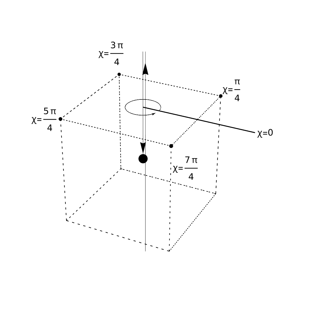
The configuration $2\pi n_{\mu\nu}(x)$ is the lattice representation of Dirac strings: a tensor field $2\pi n_{\mu\nu}$, $n_{\mu\nu}\in\mathbb{Z}$, has no effect on Wilson loops or the Wilson action. Indeed, the plaquettes with $n_{\mu\nu}\neq 0$ can be changed by a gauge transformation, but the locations of elementary cubes with nontrivial total flux of $\widetilde{n}_{\mu\nu}$ (monopole locations) cannot. For example, consider a given time slice and suppose a field $n_{ij}$ ($i,j=1,2,3$) that is nontrivial on the plaquettes pierced by a vertical line running downward from $x_{3}=+\infty$, passing through sites of the dual lattice and ending at a monopole. This is illustrated in Fig. 1, in the vicinity of the monopole. We see that $n_{12}$ equals $-1$ on the top horizontal plaquette. Now, we can perform a gauge transformation $\theta_{\mu}(x)\to\theta_{\mu}(x)+\chi(x+\hat{\mu})-\chi(x)$, where $\chi$ is the polar angle with respect to the vertical axis³³3Here, the polar angle $\chi$ is defined with a cut that does not contain any lattice site., which adds $2\pi$ to $f_{ij}$ at the plaquettes pierced by this axis, thus increasing the horizontal plaquettes $n_{12}$ by $1$ everywhere. This has the net effect of erasing the original string and creating a new one running upwards from $x_{3}=-\infty$ up to the monopole, while leaving $\bar{f}_{ij}$ invariant.

As discussed in the Introduction, a large amount of information has been gained over the years about center vortices and monopoles on the lattice. The main developments can be classified into vortex-only and monopole-only scenarios, as well as studies of their correlations.

The detection of center vortices in Yang-Mills theory, in both the direct and indirect maximal center gauges, is based on projecting gauge-fixed link variables onto the center of the gauge group.⁴⁴4The center of a group $G$ is the subgroup formed by the elements that commute with all elements of $G$. In the case of $SU(2)$, the center is the $Z(2)$ subgroup $\{\mathbb{1},-\mathbb{1}\}$. In this manner, plaquette variables computed from the projected link variables allow for the vortex detection: those yielding the nontrivial element $-\mathbb{1}$ are identified as plaquettes pierced by a center vortex (guiding center).

When it comes to monopoles, they were detected by identifying effective Abelian degrees of freedom together with a prescription similar to that developed by DeGrand and Toussaint, described in the previous subsection. More precisely, one starts by fixing the MAG via the maximization of an appropriate functional (see Section 4). In this gauge, the link variables are brought as close as possible to diagonal elements, i.e. to gauge-equivalent $SU(N)$ elements with minimal off-diagonal components. In particular, the prescription is unambiguous in the $SU(2)$ case, since there is only one diagonal generator, given by the Pauli matrix $\sigma_{3}$. Then, for each $U_{\mu}(x)\in SU(2)$, the Abelian-projected link variable $C_{\mu}(x)\in SU(2)$ is obtained as the closest diagonal group element with respect to the distance Tr$\left[\left(U_{\mu}-C_{\mu}\right)\left(U_{\mu}-C_{\mu}\right)^{\dagger}\right]$, i.e. by maximizing the overlap ${\rm Re}{\rm Tr}\left(U_{\mu}C^{\dagger}_{\mu}\right)$, where ${\rm Tr}$ is the trace in color space. This defines the Abelian-projected link variable

$$C_{\mu}(x)\,=\,e^{i\theta_{\mu}\sigma_{3}}\,=\,\left(\begin{array}[]{ccc}e^{i\theta_{\mu}(x)}&0\\ 0&e^{-i\theta_{\mu}(x)}\end{array}\right)\;,$$

(4)

which can be used to calculate the Abelian-projected plaquettes $\,C_{\mu\nu}\equiv e^{if_{\mu\nu}\sigma_{3}}$, where $f_{\mu\nu}$ is given by Eq. (1). Following this procedure, monopoles in $SU(2)$ were detected by simply applying Eq. (2) to the phase $\theta_{\mu}$ in Eq. (4). In this case, the Dirac string for an elementary monopole carries a flux $\,2\pi\,n_{\mu\nu}\,\sigma_{3}$, where $n_{\mu\nu}=\pm 1$ and the sign determines the orientation of the string. This flux contributes trivially to the (Abelian-projected) Wilson loop and action, since $e^{\pm i2\pi\sigma_{3}}=\mathbb{1}$.

As mentioned in the Introduction, it is interesting to note that a strong correlation between monopoles and vortices in $SU(2)$ was observed on the lattice [29, 49]. In the first reference, relying on the IMC gauge, it was found that 97% of the detected monopoles sit on top of vortices. It was also established that about 61% of the vortex lines have no monopoles, 31% contain a monopole-antimonopole pair, and 8% of closed vortex lines have an even number of pairs, with monopoles alternating with antimonopoles. Besides these percentages, which refer to correlations with the vortex guiding centers, correlations were also observed at the level of the full unprojected lattice. This was done by studying the action density distribution on the faces of the cube surrounding an elementary monopole. This distribution was found to be highly asymmetric, with almost all action deviations from the mean concentrated on the P-plaquettes. This asymmetry could also manifest itself in the flux distribution associated with the Abelian-projected variables, when analyzing the flux $\bar{f}_{\mu\nu}\sigma_{3}$ through the plaquette $(x,\mu,\nu)$ of a surface surrounding an elementary monopole. Instead of a uniform flux distribution, it is reasonable to expect a pair of fluxes leaving the monopole, collimated on the typical scale of the center-vortex thickness and each carrying a flux $\pi\sigma_{3}$. In particular, when computing Abelian-projected Wilson loops, encircled collimated objects would contribute a nontrivial center element $e^{\pm\pi\sigma_{3}}=-\mathbb{1}$. Here, the sign in the exponent depends on the relative orientation of the vortex and the loop. As discussed in Ref. [29], the collimation was instead explored by studying doubly charged Polyakov lines. The results showed that the Abelian-projected lattice is not described by a monopole Coulomb gas, but by a collimated center-vortex structure.

With regard to $SU(3)$, the center is the $Z(3)$ subgroup $\{\mathbb{1},e^{i2\pi/3}\mathbb{1},e^{i4\pi/3}\mathbb{1}\}$. This time, there are two nontrivial center elements. As $e^{i4\pi/3}=e^{-i2\pi/3}$, a center-vortex line characterized by a center charge $k=2$ can be thought of as a unit-charge center vortex with opposite orientation. Since the Cartan subgroup is two-dimensional, monopole detection is no longer clearly defined, and a variety of methods can be found in the literature. These methods may differ in one or more of the following three steps: (i) the MAG gauge-fixing functional, (ii) the Abelian projection, and (iii) the generalized DeGrand-Toussaint procedure.

In Ref. [31], prescriptions closely following the ones in $U(1)$ and $SU(2)$ were considered for the MAG functional and for the generalization of the DeGrand-Toussaint algorithm (see Section 3.2.) In that work, center vortices were also located using the IMC gauge. The fraction of times that $n$ faces of the cube dual to a magnetic-current link are pierced by a $Z(3)$ flux was observed and the obtained values at $\beta=6$ were $0.16(1)$ ($n=0$), $0.74(1)$ ($n=2$), $0.07(2)$ ($n=3$), $0.02(2)$ ($n=4$), $0.001(1)$ ($n=5$), and $0.001(1)$ ($n=6$). On the other hand, no studies of the action-density distribution using unprojected variables, nor of the flux distribution of Abelian-projected fluxes around monopoles, were performed.

In fact, in order to study the Abelian-projected lattice for $SU(N)$ with $N\geq 3$, it is essential to understand which fluxes generalize the $\pm\pi\sigma_{3}$ and $\pm 2\pi\sigma_{3}$ fluxes respectively carried by a collimated center vortex and a monopole in $SU(2)$. Moreover, a consistent three-step procedure should be implemented to properly detect monopoles and to map the fluxes carried along the thick collimated vortices, guided by the thin-center-vortex network detected via the IMC gauge. The objective of the next two sections is to fill this gap in the currently available detection tools, thereby opening the possibility of a deeper characterization of the confining Yang-Mills vacuum.

Studies on the Abelian-projected lattice are based on bringing the link variables $U_{\mu}\in SU(N)$ to the MAG, followed by a projection onto Cartan (diagonal) variables $C_{\mu}(x)$. As the Cartan subalgebra is $(N-1)$-dimensional, we have

$$C_{\mu}(x)\,=\,e^{i\theta_{\mu}(x)\,\cdot\,T}\,,\qquad\theta_{\mu}(x)\cdot\,T\,\equiv\;\theta_{\mu}(x)|_{q}\,T_{q}\;,$$

(5)

where the repeated index is summed over $q=1,\dots,N-1$ and $T_{q}$ are the Hermitian basis elements defined in Eq. (65). The corresponding projected plaquette variables

$\displaystyle C_{\mu\nu}(x)\,\equiv\,C_{\mu}(x)\,C_{\nu}(x+\hat{\mu})\,C^{\dagger}_{\mu}(x+\hat{\nu})\,C^{\dagger}_{\nu}(x)$

(6)

are then given by

$$C_{\mu\nu}(x)\,=\,e^{if_{\mu\nu}\,\cdot\,T}\,,\qquad f_{\mu\nu}\,\cdot\,T\,\equiv\,f_{\mu\nu}|_{q}\,T_{q}\,,\qquad f_{\mu\nu}\,=\,\partial_{\mu}\theta_{\nu}-\partial_{\nu}\theta_{\mu}\;.$$

(7)

Naturally, $f_{\mu\nu}\cdot T$ is the Cartan flux in this case and equates to the magnetic flux through the plaquette $(x,\mu,\nu)$. Notice that $\theta_{\mu}$ and $f_{\mu\nu}$ are $(N-1)$-tuples, with the components $f_{\mu\nu}|_{q}$ defined from the respective components $\theta_{\mu}|_{q}$ as in Eq. (1). Notice also that the relation between the (diagonal) elements of $C_{\mu}(x)$ and the “angles” $\theta_{\mu}(x)$ is not as direct as it was for the $SU(2)$ case.

Center vortices were detected by using the remaining $U(1)^{N-1}$ gauge symmetry to drive $C_{\mu}$ as close as possible to a $Z_{\mu}$ configuration in the center of $SU(N)$, formed by the elements

$$e^{i\frac{2\pi k}{N}}\,\mathbb{1}\,,\qquad k=0,\dots,N-1\;,$$

(8)

and looking for nontrivial plaquettes

$$Z_{\mu\nu}(x)\;=\,Z_{\mu}(x)\,Z_{\nu}(x+\hat{\mu})\,Z^{\dagger}_{\mu}(x+\hat{\nu})\,Z^{\dagger}_{\nu}(x)\;.$$

(9)

By construction, these vortices are thin. They are expected to guide the flux distribution of thick collimated objects existing before the center projection. In this respect, it is interesting to note that the $Z(N)$ fluxes do not entirely capture the complexity of collimated fluxes. For instance, consider an Abelian-projected configuration such that

$$f_{\mu\nu}\cdot T\,=\,a_{\mu\nu}\,\beta_{i}\cdot T\,,\qquad\beta_{i}\,=\,2N\,\omega_{i}\;,$$

(10)

where $\omega_{i}$, $i=1,\dots,N$, is a given weight of the defining representation (see Appendix B). Here, $\beta_{i}$ is an $(N-1)$-tuple, while the variables $a_{\mu\nu}$ are real numbers. The Wilson loop for a curve $\mathcal{C}$ on the Abelian-projected lattice is

$$\mathcal{W}_{\mathcal{C}}\,=\,e^{i\,\sum_{S}f_{\mu\nu}\cdot\,T}\;,$$

(11)

where $\sum_{S}=\sum_{(\mu\nu)\in S}$ denotes the sum over the plaquettes that form any surface $S$ whose border is $\mathcal{C}$. Now, consider a collimated distribution such that $\,\sum_{S}a_{\mu\nu}\approx\pm 2\pi$, where the sign determines how the flux is oriented in the 4D discretized spacetime. In this case, the encircled total flux and the Wilson loop are, respectively,

$$\sum_{(\mu\nu)}f_{\mu\nu}\,\approx\,\pm 2\pi\beta_{i}\cdot T\,,\qquad\mathcal{W}_{\mathcal{C}}\,\approx\,e^{\,\mp\frac{2\pi i}{N}}\;,$$

(12)

which follows from the property (see Appendix B)

$$e^{i\,2\pi\beta_{i}\cdot T}\,=\;e^{-i\>\!\frac{2\pi}{N}}\,\mathbb{1}\;.$$

(13)

That is, the contribution to $\mathcal{W}_{\mathcal{C}}$ is that of an elementary center vortex (center charge $k=+1$ or $-1$), but here it is due to a collimated Cartan flux. Furthermore, note that the $N$ different Cartan fluxes $2\pi\beta_{i}\cdot T$, $i=1,\dots,N$ correspond to one and the same center element.

We now discuss monopoles in $SU(N)$, $N\geq 3$, as motivation for our proposed detection method. The initial difficulty resides in the fact that the Cartan subalgebra has more than one dimension. Let us consider, as before, the phases associated with diagonal elements of the projected link. As noted above, such phases are not so simply connected with the variables $\theta_{\mu}(x)$ for $N\geq 3$. We therefore call them $\phi_{\mu}^{(i)}(x)$, $i=1,\cdots,N$. Usually [31], after fixing to the MAG, the diagonal part of the gauge links is extracted as in the $SU(2)$ case, by the maximization of the overlap of the diagonal field $C_{\mu}(x)$ with the complete link variable $U_{\mu}(x)$. More precisely, in $SU(3)$, if we write

$$\vskip 5.69054ptC_{\mu}(x)\,=\,\left(\begin{array}[]{ccc}e^{i\phi^{(1)}_{\mu}(x)}&0&0\\ 0&e^{i\phi^{(2)}_{\mu}(x)}&0\\ 0&0&e^{i\phi^{(3)}_{\mu}(x)}\end{array}\right)\,,\qquad\phi^{(1)}_{\mu},\;\phi^{(2)}_{\mu},\;\phi^{(3)}_{\mu}\,\in\,[0,2\pi)\;,$$

(14)

one maximizes ${\rm Re}\text{Tr}\,[U_{\mu}(x)\,C_{\mu}^{\dagger}(x)]$ with respect to the angle variables $\phi_{\mu}^{(i)}$, with the constraint $\phi^{(1)}_{\mu}+\phi^{(2)}_{\mu}+\phi^{(3)}_{\mu}=0\;\text{ mod }2\pi\,$.⁵⁵5Note that, in Ref. [31], the maximization procedure was found to be equivalent to simply extracting the phases of the three diagonal elements of $U_{\mu}(x)$ and imposing the constraint on their sum, i.e. considering each diagonal phase minus the average of the three diagonal phases. This is the procedure we implement in our comparative study in Section 5. (In [34, 35], a similar maximization was done with the two Cartan components of $C_{\mu}$ as parameters.)

We then need a new prescription to compute the monopole currents. For example, in Refs. [31, 35], the DeGrand-Toussaint method described in the previous section was applied independently to each one of the three fluxes $f^{(i)}_{\mu\nu}$ associated with $\phi_{\mu}^{(i)}$. The measured monopoles would then have a charge with three integer components $(j^{(1)}_{\mu},j^{(2)}_{\mu},j^{(3)}_{\mu})$. If we subdivide the space of the three phases into cubic cells of side $2\pi$, then, extending the prescription in Eq. (2), one considers an “initial” point $(f^{(1)}_{\mu\nu},f^{(2)}_{\mu\nu},f^{(3)}_{\mu\nu})$ in this space and takes it to a point $(\bar{f}^{(1)}_{\mu\nu},\bar{f}^{(2)}_{\mu\nu},\bar{f}^{(3)}_{\mu\nu})$, inside the unitary cubic cell centered at the origin. The path is, of course, a set of discrete steps of size $2\pi$ along each of the three directions. Note that the three flux components are treated as independent, but are in fact correlated. We refer to this as the diagonal procedure.

An alternative and non-equivalent way to proceed is to work with the natural parametrization of Cartan fluxes, given in Eqs. (5) and (7). This will lead to a mathematically sound extension of the procedure carried out for the $U(1)$ and $SU(2)$ groups, emphasizing the main structures of the Cartan subalgebra of $\mathfrak{su}(N)$. We refer to this approach as the Cartan-based procedure. In order to find the correct representation for a Dirac string in this language, let us consider a weight of the adjoint representation $\alpha_{ij}=\omega_{i}-\omega_{j}$, cf. Eq. (78), and take

$$f_{\mu\nu}\,=\,2\pi\,\beta_{ij}\,,\qquad\beta_{ij}\,=\,2N\,\alpha_{ij}\;.$$

(15)

Then we get, from the mathematical identity in Eq. (13), that

$$e^{i\!\>f_{\mu\nu}\!\>\cdot\,T}\,=\;e^{i\,2\pi\,\beta_{ij}\!\>\cdot\,T}=\,e^{i\,2\pi\,2N\,\omega_{i}\!\>\cdot\,T}\,e^{-i\,2\pi\,2N\,\omega_{j}\!\>\cdot\,T}\,=\,\mathbb{1}\;.$$

(16)

Note that this is true for any $i,j$. The tuples $\beta_{i}$ and $\beta_{ij}$ are called “magnetic” weights of the defining and adjoint representation, respectively [50]. A depiction of them for $SU(3)$ is shown in Fig. 2.

Thus, shifting a Cartan phase by elements of the lattice generated by integer combinations of $2\pi\,\beta_{ij}\cdot T$ plays a role analogous to the $2\pi$ phase periodicity of link variables in the compact Abelian case, Eq. (2). In particular, this clarifies how the DeGrand-Toussaint method can be extended⁶⁶6It is worth noting that this manner of implementing the DeGrant-Toussaint algorithm was first introduced in a previous work [36], but not in a way that assigns roots to the detected monopoles, as we will be doing soon. using the parametrization in Eq. (5): the appropriate terms that can be subtracted from the exponent in Eq. (7) in order to find $\bar{f}_{\mu\nu}$ are $2\pi\beta_{ij}$. It is worth noting that not all of them are independent and, thus, only simple roots, with $j=i+1$, need to be considered. Then, the natural way to define the DeGrand-Toussaint prescription in $\mathfrak{su}(N)$ is

$$f_{\mu\nu}\,=\,\bar{f}_{\mu\nu}+2\pi\,l_{\mu\nu}\;,$$

(17)

where $l_{\mu\nu}$ belongs to the lattice generated by $\beta_{ij}$ and is chosen such that the tuple $\bar{f}_{\mu\nu}$ lies in a unit cell, that is, a region whose translations by the lattice vectors cover $\mathbb{R}^{N-1}$ exactly once (up to boundaries). For $\mathfrak{su}(3)$, from Fig. 2, we clearly observe two main properties. First, this region can be chosen as the central hexagon (in red), scaled by a factor of $2\pi$. Second, the set of all points $b\in\mathbb{R}^{2}$ in this hexagon is characterized by having projections along the directions $\beta_{ij}/|\beta_{ij}|$ with modulus at most $|\beta_{ij}|/2$:

$$b\cdot\frac{\beta_{ij}}{|\beta_{ij}|}\,\in\,\biggl[-\frac{|\beta_{ij}|}{2},\,+\frac{|\beta_{ij}|}{2}\biggr]\;.$$

(18)

In fact, this condition also determines the unit cell for general $N$, where $b\in\mathbb{R}^{N-1}$. From Eq. (15), and using our conventions, we have $|\alpha_{ij}|=1/\sqrt{N}$, see Eq. (98) for $\mathfrak{su}(3)$. Thus, the unit cell is given by

$$\frac{1}{2}\;\bar{f}_{\mu\nu}\cdot\alpha\;\in\,[-\pi,+\pi]\;,$$

(19)

for every positive root $\alpha$. Therefore, if a plaquette variable $f_{\mu\nu}$ is a point outside the fundamental hexagon, it is taken inside the unit cell, i.e. it is moved until the condition in Eq. (19) is met, by a set of discrete steps along the directions $\beta_{ij}$. This is shown in Fig. 3.

Just as in the Abelian or $SU(2)$ case, the tensor $2\pi\,l_{\mu\nu}$ is the lattice representation of a Dirac surface. Due to Eqs. (15) and (16), it has no effect on (projected) Wilson loops or on the Wilson action. In addition, when the sum of the fluxes $2\pi l_{\mu\nu}$ through all the faces of a cube is nonzero, a monopole is detected. Of course, the sum of the fluxes $\bar{f}_{\mu\nu}$ will then be nonzero and opposite. The plaquettes with $l_{\mu\nu}\neq 0$ can be changed by a gauge transformation, while the monopole locations cannot (see Section 3.3). Thus, monopoles are the only physical degrees of freedom associated with $l_{\mu\nu}$.

Interestingly, the unit cell defined by Eq. (19) is a regular higher-dimensional polytope with vertices at $\pm 2\pi\beta_{i}$. Thus, although this construction is oriented toward detecting monopoles, it is closely related to the fluxes of elementary center vortices, as discussed in Section 3.1. This, in turn, is related to the possibility of nonoriented collimated center vortices (see Section 3.4). Of course, for $N=2$, the vertices correspond to Cartan fluxes at $\pm 2\pi\,2\alpha_{1}T_{1}=\pm\pi\sigma_{3}$, cf. Eqs. (82) and (84). These are the center-vortex fluxes around monopoles in $\mathfrak{su}(2)$, whose collimation has already been studied (see Section 2.2).

At this point, it is enlightening to compare the above described diagonal and Cartan-based procedures. Regarding the diagonal procedure, notice that the three phases in Eq. (5) are not independent, but this does not imply a strong dependence among the monopole currents $j_{\mu}^{(i)}$, which do not need to sum to $0$ themselves. This can lead to unphysical currents, even though it has been argued that they have no effect on average [31]. In any case, one should determine the best way to extract physical information from the fluxes in the exponent of the Abelian-projected variables for $N\geq 3$.

In order to discuss this in more detail, let us introduce a common notation. Both methods start from the Cartan-projected link variables parametrized as in Eq. (5) or Eq. (14), that is, with an exponent in the Cartan subalgebra, which we write as

$$C_{\mu}(x)\,=\,e^{i\Phi_{\mu}(x)}\;,\qquad{\rm Tr}(\Phi_{\mu})=0\;.$$

(20)

The corresponding projected plaquette variables are

$$C_{\mu\nu}(x)\,=\,e^{iF_{\mu\nu}(x)}\;,\qquad F_{\mu\nu}=\partial_{\mu}\Phi_{\nu}-\partial_{\nu}\Phi_{\nu}\;.$$

(21)

In principle, the physical content is encoded in the group-valued $C_{\mu\nu}$. On the other hand, monopole detection is performed at the level of the phases $F_{\mu\nu}$, which are in the Cartan subalgebra. The generalized DeGrand-Toussaint procedure defined in both cases involves a decomposition of the form

$$F_{\mu\nu}\,=\,\widebar{F}_{\mu\nu}+2\pi\,N_{\mu\nu}\;,$$

(22)

where $\widebar{F}_{\mu\nu}$ lies in a given domain and $N_{\mu\nu}$ is a diagonal matrix with integer entries, which may be constrained or unconstrained. Indeed, in the Cartan-based case, the traceless constraint is resolved by $F_{\mu\nu}=f_{\mu\nu}\cdot T$ and the decomposition $F_{\mu\nu}=\bar{f}_{\mu\nu}\cdot T+2\pi\,l_{\mu\nu}\cdot T$, as the second term is equal to ($2\pi$ times) a general traceless $N_{\mu\nu}$.⁷⁷7Note that $l_{\mu\nu}$ belongs to the lattice generated by $\beta_{ij}$ and, from Eq. (16), $\beta_{ij}\cdot T$ necessarily has integer entries.

In both methods, the monopole currents are identified through

$$j_{\mu}\,=\,-\partial_{\nu}\widetilde{N}_{\mu\nu}\,,\qquad\widetilde{N}_{\mu\nu}\,=\,\frac{1}{2}\,\epsilon_{\mu\nu\rho\sigma}\,N_{\rho\sigma}\;,$$

(23)

which is the analogue of the Abelian case in Eq. (3). Now, in the diagonal method, it is not always possible to find a traceless $N_{\mu\nu}$ such that $\widebar{F}_{\mu\nu}$ lies within the “cube” defined by constraining all three phases to the interval $[-\pi,\pi]$. Since $F_{\mu\nu}$ is Cartan-valued, the possibilities split into two cases: either both $\widebar{F}_{\mu\nu}$ and $N_{\mu\nu}$ lie in the Cartan subalgebra, or both lie outside it. In the first case, it is interesting to note that $\widebar{F}_{\mu\nu}$ coincides for both the diagonal and the Cartan-based procedures. If we show that a traceless $\widebar{F}_{\mu\nu}$, with parameters in the cube, satisfies the conditions in Eq. (19) to be inside the fundamental hexagon, then it must be true that $\widebar{F}_{\mu\nu}=\bar{f}_{\mu\nu}\cdot T$, since both decompositions are unique. In terms of $\widebar{F}_{\mu\nu}$, these conditions are

$$N\,\text{Tr}\left(\widebar{F}_{\mu\nu}\,\alpha\cdot T\right)\,\in\,[-\pi,\pi]\;,$$

(24)

for every root $\alpha$, which are differences of weights: $\alpha=\omega_{i}-\omega_{j}$, cf. Eq. (78). Then, by using Eqs. (73) and (75), it can be shown that

$$N\,\text{Tr}\left(\widebar{F}_{\mu\nu}\,\alpha\cdot T\right)\,=\,\frac{\widebar{F}_{\mu\nu}|_{ii}-\widebar{F}_{\mu\nu}|_{jj}}{2}\;,$$

(25)

where $\widebar{F}_{\mu\nu}|_{ij}$ denotes a matrix element of $\widebar{F}_{\mu\nu}$. Consequently, whenever the diagonal components of $\widebar{F}_{\mu\nu}$ are in the interval $[-\pi,\pi]$ and sum to zero, the corresponding $\bar{f}_{\mu\nu}$ is in the fundamental hexagon. Of course, if this applies to all the plaquettes of a cube, then the monopole detection will coincide on this cube. On the other hand, because of the second possibility, when following the diagonal method, monopoles may carry unphysical fluxes outside the Cartan algebra.

Our proposal directly targets the physical sector. As a side remark, note that the phases of the link variables in $\Phi_{\mu}$ are not unique. One may shift

$$\Phi_{\mu}(x)\;\to\;\Phi^{\prime}_{\mu}(x)=\Phi_{\mu}(x)+2\pi\,L_{\mu}(x)\;,$$

(26)

where $L_{\mu}(x)$ is a diagonal matrix with integer entries. In both the constrained and unconstrained cases, this integer phase transformation leaves $C_{\mu}$ and $C_{\mu\nu}$ unchanged, while inducing

$$F_{\mu\nu}\;\to\;F^{\prime}_{\mu\nu}=F_{\mu\nu}+2\pi\,(\partial_{\mu}L_{\nu}-\partial_{\nu}L_{\mu})\;.$$

(27)

As a consequence, $\widetilde{N}_{\mu\nu}$ is changed by the addition of $\epsilon_{\mu\nu\rho\sigma}\partial_{\rho}L_{\sigma}$, which is localized on closed surfaces. In the constrained case, this corresponds to large gauge transformations that change the Dirac worldsurfaces, while leaving $\widebar{F}_{\mu\nu}$ invariant. In the unconstrained case, to move the open surfaces encoded in $\widetilde{N}_{\mu\nu}$, the Cartan gauge subgroup should be enlarged to allow for large transformations carrying three independent $U(1)$ fluxes.

Finally, since our method focuses on the defining properties of the root lattice, cf. Eq. (19), which characterizes the $\mathfrak{su}(N)$ Lie algebra, it naturally encodes non-Abelian information. Moreover, it enables the detection of additional correlated objects in the Yang-Mills vacuum, as discussed in the next section.

Let us consider the elementary fluxes $2\pi\beta_{ij}\cdot T$ of monopoles on the Abelian-projected lattice, where $\beta_{ij}=\beta_{i}-\beta_{j}$ and we refer to Eq. (10). It is natural to expect the emanating flux to be collimated along a pair of attached center-vortex lines. Indeed, as discussed in Section 3.1, total fluxes $2\pi\beta_{i}\cdot T$ correspond to those carried by elementary center vortices. Such center-vortex/monopole chains are also known as nonoriented vortices and are represented in Fig. 4. On one side of the monopole, the Cartan flux, with a distribution that is locally close to $a_{\mu\nu}\,\beta_{1}\cdot T$, changes across the monopole to a distribution given locally by $a_{\mu\nu}\,\beta_{2}\cdot T$. Note that this change of orientation occurs in the Lie algebra. This is clearly the case for $N\geq 3$. In $SU(2)$, where the elementary fluxes are $\pm\pi\,\sigma_{3}$, this change may be confused with a change in spatial orientation, in which $a_{\mu\nu}$ changes sign from one side to the other.

The characterization of Cartan fluxes may also be helpful to study flux distributions around branching points in networks of vortex guiding centers, as detected by the procedure based on fixing the IMC gauge. These points have been detected in the DMC gauge by identifying cubes containing a $k=3$ center monopole, in $SU(3)$, and they constitute fundamental building blocks of the network [18]. With our method, one could also address the question of the relative frequencies of different Cartan distributions that produce the same $Z(3)$ center monopole at a junction. A possible configuration is depicted in Fig. 5, where three fluxes characterized by three different magnetic weights $\beta_{1},\beta_{2},\beta_{3}$ are matched at a point. This is possible because of the relation $\beta_{1}+\beta_{2}+\beta_{3}=0$. Such occurrence should be studied by first using the IMC gauge since, at the level of the Abelian-projected lattice, there would be no Cartan monopole at the matching point, that is, no Dirac string in the lattice data. On the other hand, a $Z(3)$ center monopole could also coincide with a Cartan monopole, which could be detected by any of the generalized DeGrand-Toussaint methods described above. For example, this would be the case when three collimated center vortices carrying flux $2\pi\beta_{1}\cdot T$ enter a monopole, which can be detected by a Dirac string carrying flux, with magnetic charge $3\beta_{1}=\beta_{12}+\beta_{13}$.

At present, there are no lattice studies of the above-mentioned flux distributions. Some indirect information about these correlations can be inferred from the results in Ref. [31] (see Section 2.2). We first note the relatively large fraction ($16\%$) of monopoles not sitting on center vortices, as compared to $3\%$ in $SU(2)$. We speculate that this may be related to spurious monopoles carrying $U(1)^{3}$-like fluxes that are not genuine Cartan fluxes. The $74\%$ fraction of Abelian-projected monopoles correlated with a pair of $P$-plaquettes would in principle be associated with nonoriented configurations. In addition, about $7\%$ of Cartan monopoles would coincide with $Z(3)$ monopoles. However, no information is available to compare the fractions of $Z(3)$ monopoles that do and do not coincide with a Cartan monopole. There is also the possibility of configurations where monopole worldlines carrying different adjoint charges meet at points on the 4D lattice. Such configurations are allowed by flux conservation. For example, three worldlines carrying adjoint magnetic fluxes $\beta_{12}$, $\beta_{23}$, and $\beta_{31}$ can meet at a point, since $\beta_{12}+\beta_{23}+\beta_{31}=0$.

In Refs. [43, 44, 45, 46, 48], all these elements —namely, oriented and nonoriented center vortices, the possibility of center-vortex $N$-matching, as well as monopole fusion— were extensively explored (for a comprehensive review, see Ref. [51]).

In particular, Ref. [43] proposed a mixed ensemble of oriented and nonoriented collimated fluxes as a mechanism for confinement. There, percolating oriented center-vortex worldsurfaces in 4D were effectively described by emergent gauge fields $\Lambda_{\mu}$, which represent the Goldstone modes in the center-vortex condensate. The nonoriented component gives rise to monopole scalar fields minimally coupled to $\Lambda_{\mu}$. In addition, the monopole condensate and monopole fusion lead to a phase with spontaneously broken symmetry. In the continuum, these are key ingredients for the generation of topologically stable confining flux tubes between quarks and for the confinement of valence gluons.

Along this line of research, Ref. [46] proposed a vacuum wave functional $\Psi[A]$ peaked at Abelian-projected center-vortex configurations. Since this approach deals with gauge fields $A(x)$ defined at a given time slice, the configurations become networks of center-vortex lines in $\mathbb{R}^{3}$. This allowed the use of a mechanism similar to that implemented in 3D spacetime in Ref. [45], but in the 3+1-dimensional theory. The resulting scaling properties of the confining string tension coincide with those derived in Ref. [52], based on the 4D effective model of Ref. [43]. The Abelian-projected configurations were also analyzed in Ref. [48], but at the level of the 4D partition function, where the sum over center-vortex worldsurfaces was formulated using a lattice matrix model.

On a Euclidean lattice, the MAG conditions are reproduced by finding the gauge configuration corresponding to the maximum of the functional⁸⁸8In Ref. [36], the authors argue in favor of a different implementation of the MAG, although the Cartan-based procedure is qualitatively independent of this choice. Nevertheless, as explained in Section 4.2, the usual definition of the MAG is especially adequate for our work.

$${\cal E}=\sum\limits_{x,\mu,q}\text{Tr }\big[U_{\mu}(x)\,T_{q}\,U^{\dagger}_{\mu}(x)\,T_{q}\big]\;$$

(32)

where $U_{\mu}(x)\in SU(N)$ is the lattice gauge link variable and $T_{q}$ are the Cartan generators, i.e. the diagonal part of the algebra (see Appendix A). As above, we have $q=1,\dots,N-1$. This is the gauge-fixing condition adopted in our work. Notice that, in the limit of small lattice spacing, the above functional reduces to (minus) that of Eq. (28).

Therefore, our problem is, given a thermalized gauge configuration $\{U_{\mu}\}$, to find the local transformation $\{g\}$, $g(x)\in SU(N)$, that will bring the link variables to $\{U^{g}_{\mu}\}$, the configuration corresponding to the extremum of the functional in Eq. (32). This is achieved with an iterative process, in which we find the gauge transformation $g(x)$ at a given lattice site $x$ that maximizes ${\cal E}(x)$ —defined by the expression in Eq. (32) considering only the terms involving $g(x)$— while, at all other sites, the associated links are kept unchanged. We then update the links connected to $g(x)$, i.e. $U_{\mu}(x)$ and $U_{\mu}(x-\hat{\mu})$, and move on to the next site, applying the procedure to all lattice sites. Since the functional in Eq. (32) is bounded from above, by repeating this process many times, we expect to reach a (local) maximum of the gauge functional. More precisely, we have

	$\displaystyle{\cal E}(x)$	$\displaystyle=$	$\displaystyle\sum_{\mu,q}\text{Tr}\,\Big[g(x)\,U_{\mu}(x)\,T_{q}\,U^{\dagger}_{\mu}(x)\,g^{\dagger}(x)\,T_{q}\,+\,g(x)\,U_{\mu}^{\dagger}(x-\hat{\mu})\,T_{q}\,U_{\mu}(x-\hat{\mu})\,g^{\dagger}(x)\,T_{q}\Big]$		(33)
		$\displaystyle=$	$\displaystyle\sum_{q}\text{Tr}\,\big[n_{q}(x)\,A_{q}(x)\big]\;,$

where we have defined⁹⁹9Note that $n_{q}(x)$ and $A_{q}(x)$ are elements of the Lie algebra $\mathfrak{su}(N)$.

$\displaystyle n_{q}(x)=g^{\dagger}(x)\,T_{q}\,g(x)\,,\quad A_{q}(x)=\sum_{\mu}\bigg[U_{\mu}(x)\,T_{q}\,U^{\dagger}_{\mu}(x)\,+\,U^{\dagger}_{\mu}(x-\hat{\mu})\,T_{q}\,U_{\mu}(x-\hat{\mu})\bigg]\;.$

(34)

Then, the problem of maximizing ${\cal E}(x)$ is that of finding $g(x)$ such that $n_{q}(x)$ is oriented as much as possible along the “direction” of $A_{q}(x)$, on average (when summing over $q$), cf. Eq. (33). Equivalently, we may maximize the functional ${\cal E}(x)$ directly, as described below.

For $SU(2)$, the contribution to the MAG functional in Eq. (33) at a site $x$ takes the form

$${\cal E}(x)\;=\frac{1}{8}\;\sum_{\mu}\,\text{Tr}\,\bigg[g(x)\,U_{\mu}(x)\,\sigma_{3}\,U^{\dagger}_{\mu}(x)\,g^{\dagger}(x)\,\sigma_{3}\,+\,g(x)\,U^{\dagger}_{\mu}(x-\hat{\mu})\,\sigma_{3}\,U_{\mu}(x-\hat{\mu})\,g^{\dagger}(x)\,\sigma_{3}\bigg]\;,$$

(35)

where $\sigma_{i}$, $i=1,2,3$ are the Pauli matrices. It is natural to treat the functional as the interaction of an effective spin $\,s(x)=g^{\dagger}(x)\,\sigma_{3}\,g(x)$ with an external magnetic field $\,h(x)=\sum_{\mu}\big[U_{\mu}(x)\,\sigma_{3}\,U^{\dagger}_{\mu}(x)+U^{\dagger}_{\mu}(x-\hat{\mu})\,\sigma_{3}\,U_{\mu}(x-\hat{\mu})\big]$, respectively associated with $n_{q}(x)$ and $A_{q}(x)$ in Eq. (34). In this way, the $SU(2)$ MAG functional assumes an identical form to that of the lattice Landau gauge functional, allowing treatment using spin-glass techniques [54, 55, 56]. Alternatively, we may work with the component form of the MAG functional [31].

Let us write

$$g(x)\,=\,g^{4}(x)\,\mathbb{1}+ig^{1}(x)\,\sigma_{1}+ig^{2}(x)\,\sigma_{2}\;,$$

(36)

where $g^{3}(x)=0$, since a residual $U(1)$ symmetry is left— i.e. we cannot fix the phase of the diagonal elements— and the links as

$$U_{\mu}(x)\,=\,u_{\mu}^{4}(x)\,\mathbb{1}+i\,u_{\mu}^{a}(x)\,\sigma_{a}\,\equiv\,u_{\mu}^{4}(x)\,\mathbb{1}+i\,\vec{u}_{\mu}(x)\cdot\vec{\sigma}\;,$$

(37)

where the color index $a$ is summed over, and we defined three-vectors with components $1,2,3$ of the appropriate quantities. Thus, the functional at $x$ assumes the form

	$\displaystyle{\cal E}(x)$	$\displaystyle=$	$\displaystyle\frac{1}{8}\sum_{\mu}\sum_{i=1,2}\bigg\{g^{4}u_{\mu}^{i}(x)+u_{\mu}^{4}(x)\,g^{i}\,-\,\Big[\vec{g}\times\vec{u}_{\mu}(x)\Big]_{i}\bigg\}^{2}\,+\,\frac{1}{8}\sum_{\mu}\Big[g^{4}u_{\mu}^{4}(x)-\vec{g}\cdot\vec{u}_{\mu}(x)\Big]^{2}$		(38)
			$\displaystyle\,+\,\bigg[U_{\mu}(x)\leftrightarrow U^{\dagger}_{\mu}(x-\hat{\mu})\bigg]\,+\,\frac{\xi}{8}\,\sum_{i=1,2,4}\Big[(g^{i})^{2}-1\Big]\;,$

where we indicate the expression obtained from substituting $U_{\mu}(x)$ by $U^{\dagger}_{\mu}(x-\hat{\mu})$ in the first line of the above equation, and we have inserted a Lagrange multiplier to guarantee that $g(x)$ is still in $SU(2)$. The extremization conditions are then given by $\,\partial{\cal E}/\partial g^{i}=0$, yielding the eigenvalue equation [57]

$$\begin{pmatrix}-C&0&A\\ 0&-C&B\\ A&B&C\end{pmatrix}\,\begin{pmatrix}g^{1}\\ g^{2}\\ g^{4}\end{pmatrix}=\;\xi\,\begin{pmatrix}g^{1}\\ g^{2}\\ g^{4}\end{pmatrix}\;,$$

(39)

where

	$\displaystyle A$	$\displaystyle=$	$\displaystyle 2\,\sum_{\mu}\Big[u_{\mu}^{1}(x)\,u_{\mu}^{4}(x)+u_{\mu}^{2}(x)\,u_{\mu}^{3}(x)\Big]\,+\,\bigg[U_{\mu}(x)\leftrightarrow U^{\dagger}_{\mu}(x-\hat{\mu})\bigg]\;,$		(40)
	$\displaystyle B$	$\displaystyle=$	$\displaystyle 2\,\sum_{\mu}\Big[u_{\mu}^{2}(x)\,u_{\mu}^{4}(x)-u_{\mu}^{1}(x)\,u_{\mu}^{3}(x)\Big]\,+\,\bigg[U_{\mu}(x)\leftrightarrow U^{\dagger}_{\mu}(x-\hat{\mu})\bigg]\;,$		(41)
	$\displaystyle C$	$\displaystyle=$	$\displaystyle\sum_{\mu}\bigg[\,\frac{1}{2}-u_{\mu}^{3}(x)\,u_{\mu}^{3}(x)-u_{\mu}^{4}(x)\,u_{\mu}^{4}(x)\bigg]\,+\,\bigg[U_{\mu}(x)\leftrightarrow U^{\dagger}_{\mu}(x-\hat{\mu})\bigg]\;.$		(42)

The eigenvector corresponding to the largest eigenvalue is the one that maximizes the functional. Hence, the gauge-transformation matrix is given by

$$g(x)\,=\,\mathcal{P}_{SU(2)}\left(A,\,B,\,0,\,C+\sqrt{A^{2}+B^{2}+C^{2}}\right)^{T}\;,$$

(43)

where $\mathcal{P}_{SU(2)}$ means projection onto the $SU(2)$ subgroup. This solves the problem in the $SU(2)$ case.

References

- [1] G. ’t Hooft, “Topology of the Gauge Condition and New Confinement Phases in Nonabelian Gauge Theories,” Nucl. Phys. B 190, 455-478 (1981) doi:10.1016/0550-3213(81)90442-9.
- [2] S. Mandelstam, “Vortices and Quark Confinement in Nonabelian Gauge Theories,” Phys. Rept. 23, 245-249 (1976) doi:10.1016/0370-1573(76)90043-0.
- [3] G. ’t Hooft, “On the Phase Transition Towards Permanent Quark Confinement,” Nucl. Phys. B 138, 1-25 (1978) doi:10.1016/0550-3213(78)90153-0.
- [4] G. ’t Hooft, “A Property of Electric and Magnetic Flux in Nonabelian Gauge Theories,” Nucl. Phys. B 153, 141-160 (1979) doi:10.1016/0550-3213(79)90595-9.
- [5] G. Mack and V. B. Petkova, “Comparison of lattice Gauge Theories with Gauge Groups Z(2) and SU(2),” Annals Phys. 123, 442 (1979) doi:10.1016/0003-4916(79)90346-4.
- [6] H. B. Nielsen and P. Olesen, “Vortex Line Models for Dual Strings,” Nucl. Phys. B 61, 45-61 (1973) doi:10.1016/0550-3213(73)90350-7.
- [7] L. Del Debbio, M. Faber, J. Giedt, J. Greensite and S. Olejnik, “Detection of center vortices in the lattice Yang-Mills vacuum,” Phys. Rev. D 58, 094501 (1998) doi:10.1103/PhysRevD.58.094501.
- [8] M. Engelhardt and H. Reinhardt, “Center projection vortices in continuum Yang-Mills theory,” Nucl. Phys. B 567, 249 (2000) doi:10.1016/S0550-3213(99)00727-0 [arXiv:hep-th/9907139 [hep-th]].
- [9] R. Bertle, M. Faber, J. Greensite and S. Olejnik, “The Structure of projected center vortices in lattice gauge theory,” JHEP 03, 019 (1999) doi:10.1088/1126-6708/1999/03/019 [arXiv:hep-lat/9903023 [hep-lat]].
- [10] R. Bertle, M. Faber, J. Greensite and S. Olejnik, “P vortices, gauge copies, and lattice size,” JHEP 10, 007 (2000) doi:10.1088/1126-6708/2000/10/007 [arXiv:hep-lat/0007043 [hep-lat]].
- [11] M. Faber, J. Greensite, S. Olejnik and D. Yamada, “The Vortex finding property of maximal center (and other) gauges,” JHEP 12, 012 (1999) doi:10.1088/1126-6708/1999/12/012 [arXiv:hep-lat/9910033 [hep-lat]].
- [12] P. de Forcrand and M. D’Elia, “On the relevance of center vortices to QCD,” Phys. Rev. Lett. 82, 4582-4585 (1999) doi:10.1103/PhysRevLett.82.4582 [arXiv:hep-lat/9901020 [hep-lat]].
- [13] M. Engelhardt, K. Langfeld, H. Reinhardt and O. Tennert, “Interaction of confining vortices in SU(2) lattice gauge theory,” Phys. Lett. B 431, 141-146 (1998) doi:10.1016/S0370-2693(98)00583-8 [arXiv:hep-lat/9801030 [hep-lat]].
- [14] T. G. Kovacs and E. T. Tomboulis, “Computation of the vortex free energy in SU(2) gauge theory,” Phys. Rev. Lett. 85, 704-707 (2000) doi:10.1103/PhysRevLett.85.704 [arXiv:hep-lat/0002004 [hep-lat]].
- [15] M. Faber, J. Greensite and S. Olejnik, “Casimir scaling from center vortices: Towards an understanding of the adjoint string tension,” Phys. Rev. D 57, 2603-2609 (1998) doi:10.1103/PhysRevD.57.2603 [arXiv:hep-lat/9710039 [hep-lat]].
- [16] K. Langfeld, “Vortex structures in pure SU(3) lattice gauge theory,” Phys. Rev. D 69, 014503 (2004) doi:10.1103/PhysRevD.69.014503 [arXiv:hep-lat/0307030 [hep-lat]].
- [17] A. Trewartha, W. Kamleh and D. Leinweber, “Connection between center vortices and instantons through gauge-field smoothing,” Phys. Rev. D 92, no.7, 074507 (2015) doi:10.1103/PhysRevD.92.074507 [arXiv:1509.05518 [hep-lat]].
- [18] J. C. Biddle, W. Kamleh and D. B. Leinweber, “Visualization of center vortex structure,” Phys. Rev. D 102, no.3, 034504 (2020) doi:10.1103/PhysRevD.102.034504 [arXiv:1912.09531 [hep-lat]].
- [19] F. Spengler, M. Quandt and H. Reinhardt, “Branching of Center Vortices in SU(3) Lattice Gauge Theory,” Phys. Rev. D 98, no.9, 094508 (2018) doi:10.1103/PhysRevD.98.094508 [arXiv:1810.04072 [hep-th]].
- [20] J. A. Mickley, D. Leinweber, and L. E. Oxman, “Structure of center-vortex matter in SU(4) Yang-Mills theory”, Phys. Rev. D 112, 014510 (2025) doi:10.1103/5d34-52zj
- [21] T. Suzuki and I. Yotsuyanagi, “A possible evidence for Abelian dominance in quark confinement,” Phys. Rev. D 42, 4257-4260 (1990) doi:10.1103/PhysRevD.42.4257
- [22] T. L. Ivanenko, A. V. Pochinsky, and M.I. Polikarpov, “Extended Abelian monopoles and confinement in the SU(2) lattice gauge theory,” Phys. Lett. B 252, 631 (1990) doi:10.1016/0370-2693(90)90497-T.
- [23] L. Del Debbio, A. Di Giacomo, M. Maggiore and S. Olejnik, “Confinement and monopoles in lattice QCD,” Phys. Lett. B 267, 254-260 (1991) doi:10.1016/0370-2693(91)91257-V
- [24] S. Hioki, S. Kitahara, S. Kiura, Y. Matsubara, O. Miyamura, S. Ohno and T. Suzuki, “Abelian dominance in SU(2) color confinement,” Phys. Lett. B 272, 326-332 (1991) [erratum: Phys. Lett. B 281, 416 (1992)] doi:10.1103/PhysRevD.42.4257
- [25] H. D. Trottier, G. I. Poulis, R. M. Woloshyn, “Gauge fixing and extended Abelian monopoles in SU(2) gauge theory in (2+1)-dimensions,” Phys. Rev. D 51, 2398 (1995) 10.1103/PhysRevD.51.2398[hep-lat/931200 [arXiv:hep-lat/9312008 [hep-lat]].
- [26] H. Shiba and T. Suzuki, “Monopoles and string tension in SU(2) QCD,” Phys. Lett. B333, 461 (1994) doi:10.1016/0370-2693(94)90168-6 [arXiv:hep-lat/9404015 [hep-lat]].
- [27] J. D. Stack, S. D. Neiman and R. J. Wensley, “String tension from monopoles in SU(2) lattice gauge theory,” Phys. Rev. D 50, 3399-3405 (1994) doi:10.1103/PhysRevD.50.3399 [arXiv:hep-lat/9404014 [hep-lat]].
- [28] G. S. Bali, V. Bornyakov, M. Muller-Preussker, K. Schilling, “Dual superconductor scenario of confinement: A Systematic study of Gribov copy effects,” Phys. Rev. D54 2863 (1996) 10.1103/PhysRevD.54.2863 [arXiv:hep-lat/9603012 [hep-lat]].
- [29] J. Ambjorn, J. Giedt and J. Greensite, “Vortex structure versus monopole dominance in Abelian projected gauge theory,” JHEP 02, 033 (2000) doi:10.1088/1126-6708/2000/02/033 [arXiv:hep-lat/9907021 [hep-lat]].
- [30] T. A. DeGrand and D. Toussaint, “Topological Excitations and Monte Carlo Simulation of Abelian Gauge Theory,” Phys. Rev. D 22 (1980), 2478 doi:10.1103/PhysRevD.22.2478
- [31] J. D. Stack, W. W. Tucker and R. J. Wensley, “The Maximal Abelian gauge, monopoles, and vortices in SU(3) lattice gauge theory,” Nucl. Phys. B 639, 203-222 (2002) doi:10.1016/S0550-3213(02)00537-0 [arXiv:hep-lat/0110196 [hep-lat]].
- [32] J. D. Stack, W. W. Tucker and R. J. Wensley, “Confinement in SU(3): Simple and generalized maximal Abelian gauge,” in: Greensite, J., Olejník, Š. (eds) Confinement, Topology, and Other Non-Perturbative Aspects of QCD. NATO Science Series, vol 83 (Springer, Dordrecht, 2002) doi:10.1007/978-94-010-0502-9_32 [arXiv:hep-lat/0205006 [hep-lat]].
- [33] W. W. Tucker and J. D. Stack, “A Generalized maximal Abelian gauge in SU(3) lattice gauge theory,” Nucl. Phys. B Proc. Suppl. 119, 721-723 (2003) doi:10.1016/S0920-5632(03)01644-X [arXiv:hep-lat/0209134 [hep-lat]].
- [34] N. Sakumichi and H. Suganuma, “Perfect Abelian dominance of quark confinement in SU(3) QCD,” Phys. Rev. D 90, no.11, 111501 (2014) doi:10.1103/PhysRevD.90.111501 [arXiv:1406.2215 [hep-lat]].
- [35] H. Suganuma and N. Sakumichi, “Monopole Dominance of Confinement in SU(3) lattice QCD,” PoS Confinement2018, 267 (2019) doi:10.22323/1.336.0267 [arXiv:1812.06827 [hep-lat]].
- [36] C. Bonati and M. D’Elia, “The Maximal Abelian Gauge in SU(N) gauge theories and thermal monopoles for N = 3,” Nucl. Phys. B 877, 233-259 (2013) doi:10.1016/j.nuclphysb.2013.10.004 [arXiv:1308.0302 [hep-lat]].
- [37] L. Del Debbio, M. Faber, J. Greensite and S. Olejnik, “Center dominance and Z(2) vortices in SU(2) lattice gauge theory,” Phys. Rev. D 55, 2298-2306 (1997) doi:10.1103/PhysRevD.55.2298 [arXiv:hep-lat/9610005 [hep-lat]].
- [38] K. Langfeld, H. Reinhardt and O. Tennert, “Confinement and scaling of the vortex vacuum of SU(2) lattice gauge theory,” Phys. Lett. B 419, 317-321 (1998) doi:10.1016/S0370-2693(97)01435-4[arXiv:hep-lat/9710068 [hep-lat]].
- [39] L. Del Debbio, M. Faber, J. Greensite and S. Olejnik, “Center dominance, center vortices, and confinement,” in: Damgaard, P.H., Jurkiewicz, J. (eds) New Developments in Quantum Field Theory. NATO Science Series: B:, vol 366 (Springer, Boston, 2002) doi:10.1007/0-306-47075-6_4 [arXiv:hep-lat/9708023 [hep-lat]].
- [40] C. Alexandrou, P. de Forcrand and M. D’Elia, “The Role of center vortices in QCD,” Nucl. Phys. A 663, 1031-1034 (2000) doi:10.1016/S0375-9474(99)00763-0 [arXiv:hep-lat/9909005 [hep-lat]].
- [41] P. de Forcrand and M. Pepe, “Center vortices and monopoles without lattice Gribov copies,” Nucl. Phys. B 598, 557-577 (2001) doi:10.1016/S0550-3213(01)00009-8 [arXiv:hep-lat/0008016 [hep-lat]].
- [42] J. Greensite, “An Introduction to the Confinement Problem” (Lecture Notes in Physics 972, Springer, 2020).
- [43] L. E. Oxman, “4D ensembles of percolating center vortices and monopole defects: The emergence of flux tubes with N-ality and gluon confinement,” Phys. Rev. D 98, no.3, 036018 (2018) doi:10.1103/PhysRevD.98.036018 [arXiv:1805.06354 [hep-th]].
- [44] L. E. Oxman, “4D ensembles of percolating center vortices and chains,” PoS Confinement2018, 054 (2019) doi:10.22323/1.336.0054 [arXiv:1812.01631 [hep-th]].
- [45] D. R. Junior, L. E. Oxman and G. M. Simões, “3D Yang-Mills confining properties from a non-Abelian ensemble perspective,” JHEP 01 (2020), 180 doi:10.1007/JHEP01(2020)180 [arXiv:1911.10144 [hep-th]].
- [46] D. R. Junior, L. E. Oxman and H. Reinhardt, “Infrared Yang-Mills wave functional due to percolating center vortices,” Phys. Rev. D 106, no.11, 114021 (2022) doi:10.1103/PhysRevD.106.114021 [arXiv:2211.03006 [hep-th]].
- [47] D. R. Junior, L. E. Oxman and G. M. Simões, “Prospecting effective Yang-Mills-Higgs models for the asymptotic confining flux tube,” Phys. Rev. D 108, no.9, 9 (2023) doi:10.1103/PhysRevD.108.094021 [arXiv:2308.07485 [hep-th]].
- [48] D. R. Junior and L. E. Oxman, “Ensembles of center vortices and chains: Insights from a natural lattice framework,” Phys. Rev. D 111, no.5, 054036 (2025) doi:10.1103/PhysRevD.111.054036 [arXiv:2411.04325 [hep-th]].
- [49] Ph. de Forcrand and M. Pepe, Nucl. Phys. B 598, 557–577 (2001) doi:10.1016/S0550-3213(01)00009-8 [arXiv:0008016 [hep-lat]].
- [50] P. Goddard, J. Nyuts and D. Olive, Nucl, “Gauge Theories and Magnetic Charge”, Phys. B 125, (1977) 1 doi:10.1016/0550-3213(77)90221-8.
- [51] D. R. Junior, L. E. Oxman and G. M. Simões, “From Center-Vortex Ensembles to the Confining Flux Tube,” Universe 7, no.8, 253 (2021) hrefhttps://doi.org/doi:10.3390/universe7080253doi.org/doi:10.3390/universe7080253 [arXiv:2106.04535 [hep-th]].
- [52] L. E. Oxman and G. M. Simões, “-Strings with exact Casimir law and Abelian-like profiles,” Phys. Rev. D 99 (2019) no.1, 016011 doi:10.1103/PhysRevD.99.016011 [arXiv:1811.11803 [hep-th]].
- [53] D. Dudal, J. A. Gracey, V. E. R. Lemes, M. S. Sarandy, R. F. Sobreiro, S. P. Sorella and H. Verschelde, “Off-diagonal mass generation for Yang-Mills theories in the maximal Abelian gauge,” Braz. J. Phys. 37, 406-418 (2007) doi:10.1590/S0103-97332007000300011 [arXiv:hep-th/0501227 [hep-th]].
- [54] T. Mendes, A. Cucchieri and A. Mihara, “Infrared Maximally Abelian Gauge,” AIP Conf. Proc. 892, no.1, 203-205 (2007) doi:10.1063/1.2714372 [arXiv:hep-lat/0611002 [hep-lat]].
- [55] A. Cucchieri and T. Mendes, “Critical slowing down in SU(2) Landau gauge fixing algorithms at beta = infinity,” Comput. Phys. Commun. 154, 1-48 (2003) doi:10.1016/S0010-4655(03)00279-0 [arXiv:hep-lat/0301019 [hep-lat]].
- [56] A. Cucchieri and T. Mendes, “Critical slowing down in SU(2) Landau gauge fixing algorithms,” Nucl. Phys. B 471, 263-292 (1996) doi:10.1016/0550-3213(96)00177-0 [arXiv:hep-lat/9511020 [hep-lat]].
- [57] M. Schröck and H. Vogt, Comput. Phys. Commun. 184, 1907-1919 (2013) doi:10.1016/j.cpc.2013.03.021 [arXiv:1212.5221 [hep-lat]].
- [58] J. E. Humphreys, Introduction to Lie Algebras and Representation Theory (Springer, New York, 1972).
- [59] Athenodorou A., Teper, M. J. High Energ. Phys. 82 (2021). doi: https://doi.org/10.1007/JHEP12(2021)082.
- [60] B. Lucini and M. Teper, JHEP 06 (2001), 050 doi: 10.1088/1126-6708/2001/06/050.
- [61] A. Cucchieri and T. Mendes, “Bloch Waves, Magnetization and Domain Walls: The Case of the Gluon Propagator **,” Universe 11, no.8, 273 (2025) doi:10.3390/universe11080273 [arXiv:2506.07730 [hep-lat]].
- [62] T. Mendes, L.E. Oxman, G.M. Simões and R.C.S. Tonhon, in preparation.