SeaEvo: Advancing Algorithm Discovery with Strategy Space Evolution
Sichun Luo1, Yi Huang2, Haochen Luo1, Fengyuan Liu1, Guanzhi Deng3, Lei Li1 Qinghua Yao1, Zefa Hu2, Junlan Feng2, Qi Liu1 1The University of Hong Kong 2JIUTIAN Research, China Mobile
3City University of Hong Kong
sichunluo2@gmail.com
Abstract
Large Language Model (LLM)-guided evolutionary search is increasingly used for automated
algorithm discovery, yet most current methods track search progress primarily through
executable programs and scalar fitness. Even when natural-language reasoning is used
through heuristic descriptions or reflection, it typically remains transient mutation context or unstructured memory, rather than organized as persistent
population-level state over strategic directions. As a result, evolutionary search can
struggle to distinguish syntactically different implementations of the same idea, preserve
lower-fitness but strategically promising directions, or detect when an entire family of
strategies has saturated.
We introduce SeaEvo, a modular strategy-space layer that turns language-level
strategic reasoning into first-class population-level evolutionary state in LLM-driven
program search. SeaEvo represents each candidate program with an explicit natural-language
strategy, clusters the archive by strategy semantics, retrieves behaviorally complementary
inspirations, and periodically navigates the strategy landscape to avoid saturated
directions.
Without modifying the underlying evolutionary algorithms, SeaEvo improves existing evolutionary backbones across algorithm discovery, systems optimization, and agent-scaffold design tasks in most settings.
Across four systems benchmarks, SeaEvo achieves a 20.6% average relative improvement, with the best single run on Prism scoring 3× higher.
These results suggest that persistent strategy representations provide a practical mechanism
for improving the effectiveness and cost-efficiency of LLM-guided evolutionary search,
pointing toward compound AI systems whose search capabilities benefit from the structured
accumulation and reuse of algorithmic strategies.
1 Introduction
Automatically discovering high-performing algorithms through
Large Language Model (LLM)-driven evolutionary search has emerged as a promising paradigm (Romera-Paredes et al., 2024; Novikov et al., 2025). By pairing LLMs as mutation operators with
programmatic evaluators, recent LLM-driven evolutionary systems iteratively propose, execute,
and refine candidate programs, achieving strong results in domains
where search spaces are combinatorially large and hand-crafted
heuristics are costly to design (Liu et al., 2024; Ye et al., 2024; Liu et al., 2025, 2026a).
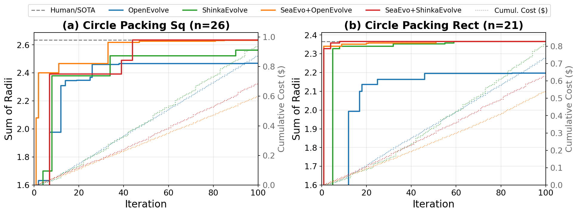
Figure 1: Search trajectories on Circle Packing benchmarks. Solid curves show the
best-so-far sum of radii over generations, dotted curves show cumulative
API cost, and the gray dashed line denotes the Human/SOTA reference.
SeaEvo improves both OpenEvolve and ShinkaEvolve backbones, reaching
competitive solutions earlier while incurring lower cumulative cost.
Despite this progress, most LLM-driven evolutionary systems still
represent search state primarily as executable programs and scalar
fitness values (Romera-Paredes et al., 2024; Novikov et al., 2025; Sharma, 2025).
Such archives support evaluation and selection, but they provide only a
limited view of search progress: different programs may instantiate the
same underlying strategy, similar scores may correspond to qualitatively
different directions, and low-scoring candidates may encode promising
ideas that have not yet been refined.
Recent work has introduced richer language-level signals, including
natural-language heuristic descriptions (Liu et al., 2024) and reflection over failures (Shinn et al., 2023; Ye et al., 2024; Agrawal et al., 2025).
However, these signals are typically used as local prompt context or
unstructured memory, rather than as a persistent population-level
representation of semantic strategy families.
This strategy-representation gap creates three practical limitations.
First, syntactically different programs may implement the same underlying idea,
making redundant variants appear as genuine search progress.
Second, selection based primarily on scalar fitness may discard lower-scoring candidates
that encode strategically useful directions or cover complementary failure modes.
Third, per-program fitness provides little visibility into strategy-family dynamics,
making it difficult to detect when an entire class of approaches has saturated.
These limitations suggest that improving LLM-guided evolution requires not only better
mutation operators or evaluators, but also a richer representation of the evolving
strategy landscape.
To address this gap, we introduce SeaEvo (Strategy-space Evolution), which elevates natural-language strategy to a first-class population-level representation in LLM-driven evolutionary program search.
SeaEvo augments each candidate with an explicit natural-language
strategy description and embedding, yielding a dual-space archive
organized by both executable programs and semantic strategies.
It consists of three coordinated modules: Strategy Articulation
(SA), which diagnoses failures and specifies a strategic direction
before code generation; Stratified Experience Retrieval (SER),
which clusters the archive in strategy space and retrieves behaviorally
complementary inspirations; and Strategic Landscape Navigation
(SLN), which summarizes effective, saturated, and underexplored
strategy families to guide future mutations.
These modules turn the archive from a flat record of programs
into a navigable map of algorithmic ideas.
We evaluate SeaEvo across mathematical algorithm discovery, systems
optimization, and agent-scaffold design benchmarks, using diverse backbone
LLMs and base evolutionary
frameworks.
SeaEvo improves the underlying backbones in most settings, with the largest gains on open-ended systems optimization tasks where qualitatively distinct strategy families exist.
Beyond this aggregate gain, SeaEvo also improves the search frontier: Figure 1 shows that it reaches competitive solutions in fewer generations while incurring lower cumulative API cost.
Case studies in Appendix F further show that strategy-space guidance can redirect evolution away from saturated local refinements toward qualitatively different algorithmic families.
These results suggest that persistent strategy representations provide a practical mechanism for improving the effectiveness and efficiency of LLM-guided evolutionary search.
Contributions.
Our contributions are as follows:
1) We identify a strategy-representation gap in LLM-guided evolutionary search:
existing archives organize search state around programs and scalar fitness scores, but do
not maintain a population-level semantic representation of the strategies being explored.
2) We introduce SeaEvo, a modular strategy-space layer that turns natural-language
strategies into persistent population-level evolutionary state through strategy descriptions,
semantic clustering, behaviorally complementary retrieval, and landscape-level navigation
over effective, saturated, and underexplored strategy families.
3) Extensive experiments across mathematical algorithm discovery,
systems optimization, and agent-scaffold design benchmarks demonstrate the effectiveness of SeaEvo. SeaEvo improves multiple
open evolutionary backbones in most settings, with a 20.6% average relative improvement across four
systems
optimization tasks.
2 Related Work
LLM-Driven Evolutionary Algorithm Discovery.
Recent work frames algorithm and program improvement as an evolutionary loop in which LLMs act as proposal or mutation operators (Van Stein and Bäck, 2024; Liu et al., 2026b). FunSearch (Romera-Paredes et al., 2024) established this paradigm by pairing an LLM with a programmatic evaluator to evolve mathematical functions, while AlphaEvolve (Novikov et al., 2025) scaled it to full codebases using a Gemini ensemble and a MAP-Elites-inspired program database (Mouret and Clune, 2015). Subsequent systems improve the efficiency and dynamics of this loop through mechanisms such as adaptive parent sampling and novelty rejection in ShinkaEvolve (Lange et al., 2025), island-based genetic operators in CodeEvolve (Assumpção et al., 2025), hierarchical context management and backtracking in PACEvolve (Yan et al., 2026), and adaptive budget and exploration control in AdaEvolve (Cemri et al., 2026). These methods primarily improve how programs are sampled, mutated, selected, or orchestrated. SeaEvo addresses a complementary axis: what the evolutionary state represents. Rather than replacing the base loop, it augments the archive with persistent strategy descriptions, semantic strategy clusters, and LLM-driven landscape navigation, making it compatible with existing evolutionary backbones.
Strategy, Reflection, and Memory in LLM-Based Heuristic Evolution.
A closely related line of work introduces language-level reasoning into optimization and evolutionary search (Yuksekgonul et al., 2025; Lee et al., 2025). EoH (Liu et al., 2024) co-evolves natural-language thoughts alongside code; ReEvo (Ye et al., 2024), Reflexion (Shinn et al., 2023), and GEPA (Agrawal et al., 2025) use verbal feedback or reflection to improve future proposals. Other systems maintain reusable insights (Chen et al., 2025), abstractions (Wu et al., 2025), or evolution strategies (Yang et al., 2025b). These works show that natural language can provide useful intermediate structure between scalar feedback and executable code. SeaEvo builds on this direction but differs in how the language signal is organized and used: prior systems typically attach thoughts, reflections, insights, or recommendations to individual candidates, lineages, or textual memories, whereas SeaEvo organizes the full archive into semantic strategy clusters, retrieves inspirations by behavioral complementarity, and tracks strategy-family dynamics at the population level. This makes strategy space a structured object of search rather than only a source of prompt content.
Figure 2: Overview of SeaEvo.
SeaEvo replaces the default context builder with a strategy-aware pipeline, while leaving the base loop’s selection and evaluation unchanged.
Three modules enrich the evolutionary loop: Strategy Articulation replaces blind mutation with a diagnose-direct-implement pipeline; Stratified Experience Retrieval assembles context from semantically clustered, behaviorally diverse archive entries; Strategic Landscape Navigation periodically diagnoses which strategy families are effective, saturated, or underexplored, and guides future mutations accordingly.
3 Method
3.1 Problem Formulation
We consider the problem of automatically discovering a high-performing
program for a given task.
Let be an evaluation metric over a
space of candidate programs . The goal is to discover
(1)
where measures task-specific fitness. In an evolutionary framework,
at generation an archive with
is maintained under a fixed capacity: an LLM prompt is
constructed from selected entries via context builder, a new candidate is generated and
evaluated, and then the archive is updated.
Existing frameworks track search progress only through code and scalar
fitness, or attach natural-language reflections as transient prompt
context without persisting them at the archive level. Neither representation
exposes which strategic directions have been explored, which remain
underrepresented, and which have already saturated. SeaEvo addresses
this by augmenting each archive entry with a persistent strategy
description and embedding, organizing the archive as a navigable map of
algorithmic ideas rather than a flat record of programs.
3.2 Framework Overview
Figure 2 illustrates SeaEvo. The method is a
modular layer that can be added on top of an existing LLM-driven
evolutionary framework: it replaces the framework’s default context
builder with a strategy-aware pipeline and augments each archive
entry with a persistent strategy description and embedding, while
leaving the base loop’s parent selection and evaluation mechanisms unchanged.
At each generation, the base framework selects a parent program.
SER retrieves strategy-level inspirations from the strategy-augmented archive;
SLN provides landscape-level guidance summarizing effective, saturated, and
underexplored strategy families; and SA uses the parent, retrieved inspirations,
and landscape guidance to generate a new program together with its strategy
description. After evaluation, the strategy description is embedded and the new
entry is inserted into the archive.
The three modules operate at different timescales. SA runs at every
strategy-guided generation. SER uses a warm-up fallback for the
first generations and switches to cluster-based retrieval once
enough strategy diversity has accumulated. SLN runs every
generations and its guidance persists between updates. All modules
operate through the context construction stage: the base framework
still sample, evaluates, and selects programs in the usual way,
while SeaEvo changes how mutation context is assembled and what
strategic state the archive maintains.
Exploration ratio.
To avoid over-constraining the search by the current strategy
representation, SeaEvo uses an -greedy scheme: with
probability it bypasses SA, SER, and SLN and falls back to
the base framework’s default mutation pipeline; with probability
it executes the full SeaEvo pipeline. This design balances strategy-guided exploitation with unguided exploration.
3.3 Strategy Articulation
Vanilla LLM mutation often leaves the search direction implicit: the model is
asked to improve a program, but the failure mode and intended algorithmic change
are not explicitly represented (Sharma, 2025). SA makes this reasoning explicit by asking the
LLM to first articulate a strategic direction before implementing code. Given a
selected parent program , an inspiration set
, and optional landscape guidance , SA produces
a new program and a strategy description using a single structured
LLM prompt.
The prompt follows a diagnose–direct–implement format.
First, the LLM diagnoses the limitations of using the
evaluation signals available to the underlying evolutionary framework, such as
scalar fitness, execution errors, or task-specific feedback when provided. SA does not require a specific feedback format: in scalar-only
settings, the diagnosis is based on the parent score, the retrieved strategy
inspirations, and the task objective; when richer feedback is available, it can
be included as additional context. Second, conditioned on this diagnosis,
, and optional SLN guidance , the LLM proposes a
concise strategy description for the next candidate. When is
available, it can steer the proposal away from saturated strategy families and
toward underexplored alternatives. Finally, the LLM implements a new program
following the proposed strategy description. The diagnosis is used only as
intermediate prompt context. After evaluation, the and
persist in the archive, with embedded for downstream clustering and
retrieval.
This design makes strategy descriptions reusable beyond the immediate mutation
step. Rather than treating reflection as transient prompt content, SA converts
each proposed direction into persistent archive state that can later be clustered
by SER and summarized by SLN.
3.4 Stratified Experience Retrieval
Many evolutionary frameworks construct mutation context by selecting
high-fitness programs or recent ancestors and using their source code as
inspiration for the next mutation (Novikov et al., 2025; Lange et al., 2025).
While code-level inspiration provides useful implementation details, it is also
costly and noisy: programs can span hundreds of lines, and syntactic similarity
does not necessarily reflect shared algorithmic intent. Moreover, fitness-based
selection can introduce a self-reinforcing bias, in which high-scoring strategy
families are repeatedly surfaced while strategically distinct but temporarily
lower-scoring candidates receive little exposure. SER addresses these issues by
organizing the archive in strategy-embedding space and retrieving inspirations
that cover both similar and distinct strategy
families while remaining behaviorally complementary.
Strategy clustering.
SER partitions the archive into strategy clusters
over strategy embeddings (Lloyd, 1982), recomputed at every generation.
This groups syntactically different programs that instantiate similar
algorithmic ideas into the same strategy family, providing the semantic
structure for retrieval.
During the warm-up stage (), when the archive is too small for reliable
clustering, SER bypasses the cluster structure and returns the parent,
the global best, and the program with the highest complementary
coverage relative to the global best.
Complementary Coverage Score.
SER ranks candidate inspirations by how many of the reference
program’s failures a candidate can solve.
Given a reference program and a fixed validation
set , each program has a binary success vector
.
We define the Complementary Coverage score (ComCov) of with respect to
is
(2)
i.e., the fraction of validation instances that
fails but solves.
ComCov rewards candidates
that cover the reference program’s failures, making retrieval complementary to
the parent’s weaknesses rather than merely diverse.
When only a scalar fitness is available (e.g., in geometric
optimization tasks where instance-level success vectors are undefined),
ComCov is identically zero and ranking falls back to fitness via the
lexicographic tiebreaker
.
Inspiration selection.
SER anchors retrieval on the parent program
chosen by the base framework.
After warm-up (), let denote the cluster
containing .
SER selects two inspirations greedily to maximize marginal
complementary coverage:
(3)
(4)
where counts only instances failed by
both and , ensuring
non-redundant coverage.
The intra-cluster pick identifies a sibling that shares the parent’s
strategic family but covers different failure cases; the cross-cluster
pick then targets the residual failures that neither the parent nor
the sibling can solve.
Random cluster sampling for , rather than a global argmax, prevents
the cross-cluster slot from being monopolized by a single dominant
family, spreading exposure across the strategy landscape over
successive generations.
For the two retrieved inspirations, SER passes only their strategy
descriptions and fitness scores, not their source code.
This reduces the inspiration portion of the prompt by one to two
orders of magnitude and forces the mutation LLM to reason at the
level of algorithmic ideas rather than copy code fragments.
3.5 Strategic Landscape Navigation
SER diversifies the local mutation context, but search may still concentrate
within a small number of strategy families. SLN adds a slower-timescale
mechanism that summarizes the population-level strategy landscape and guides
future mutations away from saturated regions.
Every generations, SLN collects the strategy descriptions and fitness
scores of programs in the current archive and passes them to an LLM. The LLM
produces structured landscape guidance with four components:
(i) effective directions: strategy families showing consistent
improvement and worth further exploitation;
(ii) saturated directions: families that appear to have plateaued and
should be de-emphasized;
(iii) underexplored directions: plausible approaches not yet well
represented in the archive; and
(iv) concrete guidance: actionable suggestions for subsequent mutation
steps.
The resulting is appended to the SA prompt and remains active
until the next SLN update.
This design treats saturation and opportunity detection as a semantic
landscape-analysis problem rather than a fixed scalar rule. By reasoning over
strategy descriptions together with their fitness trends, SLN can identify
families that are repeatedly refined without further improvement and suggest
qualitatively different alternatives that would be difficult to recover from
fitness values alone.
4 Experiments
4.1 Experiment Setup
Tasks and datasets.
We evaluate on three task families: (i) four mathematical optimization tasks, including Circle Packing in Square,
Circle Packing in Rectangle, Heilbronn Triangles, and MinMax
Distance; (ii) four systems optimization tasks
from the ADRS benchmark (Cheng et al., 2025): Prism, TXN, EPLB,
and LLM-SQL; and (iii) agent-scaffold optimization tasks.
Baselines.
We compare SeaEvo against state-of-the-art LLM-driven evolutionary
methods, including GEPA (Agrawal et al., 2025),
OpenEvolve (Sharma, 2025), and
ShinkaEvolve (Lange et al., 2025).
We instantiate two variants of our method: SeaEvo
over ShinkaEvolve, and SeaEvo over OpenEvolve;
the corresponding backbone rows therefore serve as direct ablations
of the strategy-aware modules.
For readability, figures use the expanded form (e.g., SeaEvo +ShinkaEvolve) while tables use the compact notation (e.g., SeaEvo).
We additionally apply SeaEvo to GEPA and to AdaEvolve (Cemri et al., 2026) in
Appendix E to test plug-in generality.
Implementation details.
We use two backbone LLMs as the mutation model within the evolutionary
loop: MiMo-V2-Pro (Xiaomi MiMo Team, 2026) and
Gemini-3-Flash (Google DeepMind, 2025).
For the agent-scaffold task,
the inference model is Qwen3-8B (Yang et al., 2025a).
Strategy embeddings use
text-embedding-3-small model (OpenAI, 2024) .
We build on the SkyDiscover
framework (Liu et al., 2026c). Each configuration runs for
generations with SLN update interval ,
strategy clusters, and -greedy ratio .
We use the default hyperparameters for all baseline methods.
Similar to Cemri et al. (2026), each experiment is repeated three times; we report mean and standard
deviation.
More details
are provided in Appendix D.
Table 1: Performance on mathematical optimization benchmarks.
Avg denotes mean score with standard deviation over 3 runs, and Best denotes the best score achieved.
Best results within each backbone group are bolded, and full-precision near ties are reported in Table 7.
Method
Circle Packing (Rect)
Circle Packing (Square)
Heilbronn (Triangles)
MinMax Distance
Avg
Best
Avg
Best
Avg
Best
Avg
Best
Backbone: MiMo-V2-Pro
GEPA
2.3398
2.3584
2.5206
2.5414
0.0265
0.0273
0.2760
0.2776
OpenEvolve
2.1380
2.3530
2.4003
2.4390
0.0250
0.0281
0.2564
0.2760
ShinkaEvolve
2.3560
2.3608
2.4812
2.5123
0.0272
0.0273
0.2776
0.2783
SeaEvo
2.3607
2.3642
2.6045
2.6263
0.0314
0.0330
0.2778
0.2781
SeaEvo
2.3603
2.3640
2.5467
2.6237
0.0274
0.0285
0.2780
0.2784
Backbone: Gemini-3-Flash
GEPA
2.3610
2.3621
2.5306
2.5574
0.0303
0.0316
0.2785
0.2785
OpenEvolve
2.1713
2.1968
2.4522
2.4887
0.0062
0.0087
0.2765
0.2774
ShinkaEvolve
2.3625
2.3658
2.5204
2.5617
0.0317
0.0331
0.2783
0.2785
SeaEvo
2.3643
2.3658
2.5802
2.6317
0.0305
0.0309
0.2785
0.2785
SeaEvo
2.3639
2.3658
2.6297
2.6353
0.0335
0.0342
0.2785
0.2785
Table 2: Performance on systems optimization benchmarks with Gemini-3-Flash.
Avg denotes mean score with standard deviation over runs, and Best denotes the best score achieved.
The Human/SOTA row reports reference best scores when available.
Best method results are highlighted in boldface.
Method
Prism
TXN
EPLB
LLM-SQL
Avg
Best
Avg
Best
Avg
Best
Avg
Best
Human/SOTA
–
21.89
–
2725
–
0.1265
–
0.692
GEPA
23.6733
24.0217
3266.0
3496.5
0.1472
0.1543
0.7158
0.7233
OpenEvolve
24.0217
24.0217
3586.7
3745.3
0.1260
0.1262
0.7117
0.7241
ShinkaEvolve
26.2672
26.5369
3480.7
3508.8
0.1326
0.1454
0.6998
0.7181
SeaEvo
26.1783
26.2783
3810.6
4098.4
0.1535
0.1716
0.7104
0.7114
SeaEvo
43.6149
78.0040
3886.1
4219.4
0.1958
0.1960
0.7200
0.7318
4.2 Main Results
Tables 1 and 2 report
results on mathematical and systems optimization benchmarks,
respectively. Figure 3 and 6 report agent-scaffold design results, and Figure 1 shows search trajectories on the
two Circle Packing benchmarks. We highlight several observations.
Consistent improvement across tasks and backbones.
Across most configurations in Tables 1
and 2, SeaEvo achieves the highest average fitness, and no baseline systematically dominates
on any task or backbone. The relative ranking is stable between
MiMo-V2-Pro and Gemini-3-Flash, suggesting
that gains stem from the strategy-aware modules rather than
backbone-specific behavior. The same pattern holds on the agent-scaffold design
task (see Figure 3 and 6), where SeaEvo improves both OpenEvolve
and ShinkaEvolve backbones.
Gains scale with strategy-space openness.SeaEvo’s advantage is largest on systems optimization benchmarks. SeaEvo achieves a
32.1% average relative improvement in Avg score over its ShinkaEvolve backbone across the four ADRS benchmarks. On the high-variance Prism benchmark, one run discovers a substantially stronger solution, yielding a near-3× best-score improvement over ShinkaEvolve.
Improvements are more moderate on
mathematical tasks (e.g., on Circle Packing Square Avg in
Table 1), and diminish on narrower-solution-space
tasks such as LLM-SQL. We attribute this gradient to SLN and SER
providing stronger signal when qualitatively distinct strategy
families exist to be discovered and distinguished; when the strategy
space is constrained, fitness-only baselines are harder to improve
upon.
Faster convergence at lower cost.
Figure 1 shows search trajectories on the Circle
Packing benchmarks. Both SeaEvo and SeaEvo reach the
Human/SOTA reference earlier than their underlying backbones. On
Circle Packing (Square), SeaEvo crosses within
generations whereas OpenEvolve plateaus near throughout
generations. The cumulative-cost curves show that SeaEvo’s
API cost grows slower than the backbones’, so the gains do not
come from additional compute per generation; they come from reaching
better solutions in fewer generations.
Table 3: Ablation study on Circle Packing (Square) with Gemini-3-Flash.
We report mean fitness score (Avg), standard deviation (Std), best score
(Best), generation at which best was found (Gen@Best), and average
API cost (AvgCost) across three seeds.
We highlight the best and worst values for
each metric in green and red, respectively.
SA
SER
SLN
Avg
Std
Best
Gen@Best
AvgCost
✗
✗
✗
2.5023
0.0086
2.5099
99
$0.5367
✓
✗
✗
2.5043
0.0855
2.6310
67
$0.6062
✗
✓
✗
2.5224
0.0731
2.6310
95
$0.5088
✗
✗
✓
2.5634
0.0791
2.6356
61
$0.5614
✓
✓
✗
2.5172
0.0774
2.6304
59
$0.6576
✓
✗
✓
2.5870
0.0816
2.6308
93
$0.7147
✗
✓
✓
2.5901
0.0724
2.6360
88
$0.5731
✓
✓
✓
2.6297
0.0077
2.6353
44
$0.7075
Table 4: Hyperparameter sensitivity on Circle Packing (Square) with
Gemini-3-Flash. Baseline is the full SeaEvo configuration
(, , ). Each row varies one
hyperparameter while holding the others fixed. The best results are in boldface.
Param
Value
Avg
Std
Best
Gen@Best
AvgCost
(SLN interval)
2.5628
0.1195
2.6343
80
$0.7710
2.6297
0.0077
2.6353
44
$0.7075
2.5742
0.0854
2.6307
74
$0.6802
(clusters)
2.6283
0.0052
2.6343
86
$0.7006
2.6297
0.0077
2.6353
44
$0.7075
2.6175
0.0173
2.6307
72
$0.7079
(Exploration ratio)
2.6341
0.0020
2.6360
78
$0.7711
2.6297
0.0077
2.6353
44
$0.7075
2.6263
0.0112
2.6360
95
$0.6669
4.3 Ablation Study
Table 3 reports ablation results on Circle Packing
(Square) with Gemini-3-Flash. All three modules improve over the
no-module baseline, but with distinct roles. SA and SER individually
yield modest gains in average fitness while substantially raising the
best fitness, suggesting they primarily expand the reachable solution
space. SLN alone produces the largest standalone improvement in
average fitness and the earliest convergence, indicating that
landscape-level guidance provides the strongest global search signal.
The full SeaEvo achieves the best average fitness, finds its best
solution earliest, and most strikingly reduces variance by an
order of magnitude relative to every two-module variant, reflecting a
non-additive synergy among the three modules. Notably, the SA+SER
configuration underperforms either module alone in average fitness:
without SLN’s landscape signal, structured mutation paired with
diversity-aware retrieval can over-commit to a narrow set of
directions. This pattern suggests that SLN’s role is not merely
additive but corrective, it prevents the other two modules from
locking onto premature strategy families.
4.4 Hyperparameter Sensitivity
Table 4 reports sensitivity to three key
hyperparameters on Circle Packing (Square).
SLN update interval .
achieves the best average fitness and earliest
convergence. Updating too frequently () destabilizes search:
the landscape changes before the population has accumulated enough new
candidates to make the LLM’s judgments
reliable, producing the highest variance across all settings.
Updating too infrequently () reduces cost but lets
ineffective directions persist past the point where they should be
abandoned, hurting average fitness.
Number of clusters .
Performance is robust around , with modest degradation at
(coarser strategy partitioning conflates distinct families) and
(too few programs per cluster make intra-cluster retrieval less
informative). The low sensitivity across this range suggests that
SeaEvo does not require careful tuning of .
Exploration ratio .
(fully strategy-guided, no random exploration) reaches
the highest best score but does so substantially later than
, indicating that occasional fallbacks to the base
mutation pipeline accelerate escape from premature strategy clusters.
dilutes the strategy-aware pipeline too aggressively,
hurting both average fitness and convergence speed.
provides the best balance of guided exploration and stochastic
diversity.
Figure 3: Performance on the agent scaffold design benchmark with maximum one LLM call. Bars show average test score with standard deviation across runs, and diamonds indicate the best score.
Figure 4: Strategy embedding spaces on two systems optimization benchmarks. Each point denotes a candidate program projected from its strategy embedding by t-SNE, color indicates the combined score, and marker shape distinguishes the base backbone from SeaEvo-augmented search.
4.5 Visualization
To examine whether SeaEvo changes the distribution of explored strategies rather than merely improving the final score, we project the strategy text associated with all generated programs into two dimensions using t-SNE (Van der Maaten and Hinton, 2008). For SeaEvo, this text is the explicit strategy description stored in the archive; for the ShinkaEvolve baseline, which does not maintain such descriptions, we approximate it using docstrings and comments extracted from each generated program. Figure 4 shows the resulting qualitative projections on two representative systems optimization benchmarks, EPLB and TXN Scheduling. Each point denotes one generated program; marker shape distinguishes ShinkaEvolve from SeaEvo, and color encodes the combined score.
The projections reveal a clear difference in the regions explored by the two search processes. On EPLB, ShinkaEvolve candidates concentrate in a few broad regions, whereas SeaEvo produces a dense group of high-scoring candidates in a different part of the strategy space. This suggests that the improvement is associated with discovering and refining a distinct strategy family, rather than only isolated high-scoring mutations. On TXN Scheduling, ShinkaEvolve again concentrates in a small number of regions, while the top SeaEvo candidates appear in a separate area of the projection. This is consistent with the intended role of SLN: redirecting mutations toward underexplored strategy families when local directions begin to saturate.
5 Conclusion
We introduced SeaEvo, a persistent strategy-space layer that turns
language-level strategic reasoning into population-level evolutionary
state. By associating each candidate program with a natural-language
strategy description, clustering the archive by strategy semantics,
retrieving behaviorally complementary inspirations, and monitoring
strategy-family saturation, SeaEvo transforms the archive from a flat
record of programs into a navigable map of algorithmic ideas. Across
mathematical algorithm discovery, systems optimization, and agent-scaffold
benchmarks, SeaEvo improves existing evolutionary backbones in most
settings, with the largest gains on open-ended tasks. It also improves the
search frontier by reaching competitive solutions in fewer generations
and at lower cumulative API cost. These results point toward LLM-guided
evolutionary systems that improve over time by accumulating, organizing,
and reusing algorithmic strategies.
References
L. A. Agrawal, S. Tan, D. Soylu, N. Ziems, R. Khare, K. Opsahl-Ong, A. Singhvi, H. Shandilya, M. J. Ryan, M. Jiang, C. Potts, K. Sen, A. G. Dimakis, I. Stoica, D. Klein, M. Zaharia, and O. Khattab (2025)GEPA: reflective prompt evolution can outperform reinforcement learning.
arXiv preprint arXiv:2507.19457.
Cited by: §D.2,
§E.1,
§1,
§2,
§4.1.
H. Assumpção, D. Ferreira, L. Campos, and F. Murai (2025)Codeevolve: an open source evolutionary coding agent for algorithm discovery and optimization.
arXiv preprint arXiv:2510.14150.
Cited by: §2.
M. Cemri, S. Agrawal, A. Gupta, S. Liu, A. Cheng, Q. Mang, A. Naren, L. E. Erdogan, K. Sen, M. Zaharia, A. Dimakis, and I. Stoica (2026)Adaevolve: adaptive llm driven zeroth-order optimization.
arXiv preprint arXiv:2602.20133.
Cited by: §E.1,
§2,
§4.1,
§4.1.
C. Chen, M. Zhong, Y. Fan, J. Shi, and J. Sun (2025)Hifo-prompt: prompting with hindsight and foresight for llm-based automatic heuristic design.
arXiv preprint arXiv:2508.13333.
Cited by: §2.
A. Cheng, S. Liu, M. Z. Pan, Z. Li, B. Wang, A. Krentsel, T. Xia, M. Cemri, J. Park, S. Yang, J. Chen, L. A. Agrawal, A. Desai, J. Xing, K. Sen, M. Zaharia, and I. Stoica (2025)Barbarians at the gate: how AI is upending systems research.
arXiv preprint arXiv:2510.06189.
Cited by: §D.1,
§4.1.
W. Kwon, Z. Li, S. Zhuang, Y. Sheng, L. Zheng, C. H. Yu, J. Gonzalez, H. Zhang, and I. Stoica (2023)Efficient memory management for large language model serving with pagedattention.
In Proceedings of the 29th symposium on operating systems principles,
pp. 611–626.
Cited by: §D.2.
R. T. Lange, Y. Imajuku, and E. Cetin (2025)Shinkaevolve: towards open-ended and sample-efficient program evolution.
arXiv preprint arXiv:2509.19349.
Cited by: §D.2,
§2,
§3.4,
§4.1.
Y. Lee, J. Boen, and C. Finn (2025)Feedback descent: open-ended text optimization via pairwise comparison.
arXiv preprint arXiv:2511.07919.
Cited by: §2.
T. Li, Y. Wang, Z. Chen, Z. Wang, L. Ma, and G. Qi (2025)C-evolve: consensus-based evolution for prompt groups.
arXiv preprint arXiv:2509.23331.
Cited by: §D.2.
F. Liu, T. Xialiang, M. Yuan, X. Lin, F. Luo, Z. Wang, Z. Lu, and Q. Zhang (2024)Evolution of heuristics: towards efficient automatic algorithm design using large language model.
In International Conference on Machine Learning,
pp. 32201–32223.
Cited by: §1,
§1,
§2.
F. Liu, Y. Yao, P. Guo, Z. Yang, X. Lin, Z. Zhao, X. Tong, K. Mao, Z. Lu, Z. Wang, and Q. Zhang (2026a)A systematic survey on large language models for algorithm design.
ACM Computing Surveys58 (8), pp. 1–32.
Cited by: §1.
F. Liu, H. Yi, S. Luo, Y. Wang, Y. Yang, X. Li, Z. Hu, J. Feng, and Q. Liu (2025)Cognitive alpha mining via llm-driven code-based evolution.
arXiv preprint arXiv:2511.18850.
Cited by: §1.
S. Liu, S. Agarwal, M. Maheswaran, M. Cemri, Z. Li, Q. Mang, A. Naren, E. Boneh, A. Cheng, M. Z. Pan, A. Du, K. Keutzer, A. G. Dimakis, K. Sen, M. Zaharia, and I. Stoica (2026b)EvoX: meta-evolution for automated discovery.
CoRRabs/2602.23413.
External Links: Link,
Document,
2602.23413Cited by: §2.
S. Liu, M. Cemri, S. Agarwal, A. Krentsel, A. Naren, Q. Mang, Z. Li, A. Gupta, M. Maheswaran, A. Cheng, M. Pan, E. Boneh, K. Ramchandran, K. Sen, A. G. Dimakis, M. Zaharia, and I. Stoica (2026c)SkyDiscover: a flexible framework for ai-driven scientific and algorithmic discovery.
External Links: LinkCited by: §4.1.
S. Lloyd (1982)Least squares quantization in pcm.
IEEE transactions on information theory28 (2), pp. 129–137.
Cited by: §3.4.
J. Mouret and J. Clune (2015)Illuminating search spaces by mapping elites.
arXiv preprint arXiv:1504.04909.
Cited by: §2.
A. Novikov, N. Vu, M. Eisenberger, E. Dupont, P. Huang, A. Z. Wagner, S. Shirobokov, B. Kozlovskii, F. J. R. Ruiz, A. Mehrabian, M. P. Kumar, A. See, S. Chaudhuri, G. Holland, A. Davies, S. Nowozin, P. Kohli, and M. Balog (2025)AlphaEvolve: A coding agent for scientific and algorithmic discovery.
arXiv preprint arXiv:2506.13131.
Cited by: §D.2,
§1,
§1,
§2,
§3.4.
V. Pyatkin, S. Malik, V. Graf, H. Ivison, S. Huang, P. Dasigi, N. Lambert, and H. Hajishirzi (2025)Generalizing verifiable instruction following.
In The Thirty-ninth Annual Conference on Neural Information Processing Systems Datasets and Benchmarks Track,
Cited by: §D.1.
B. Romera-Paredes, M. Barekatain, A. Novikov, M. Balog, M. P. Kumar, E. Dupont, F. J. R. Ruiz, J. S. Ellenberg, P. Wang, O. Fawzi, P. Kohli, and A. Fawzi (2024)Mathematical discoveries from program search with large language models.
Nat.625 (7995), pp. 468–475.
External Links: Link,
DocumentCited by: §1,
§1,
§2.
P. Röttger, H. Kirk, B. Vidgen, G. Attanasio, F. Bianchi, and D. Hovy (2024)Xstest: a test suite for identifying exaggerated safety behaviours in large language models.
In Proceedings of the 2024 Conference of the North American Chapter of the Association for Computational Linguistics: Human Language Technologies (Volume 1: Long Papers),
pp. 5377–5400.
Cited by: §D.1.
A. Sharma (2025)OpenEvolve: an open-source evolutionary coding agentExternal Links: LinkCited by: §D.2,
§1,
§3.3,
§4.1.
N. Shinn, F. Cassano, A. Gopinath, K. Narasimhan, and S. Yao (2023)Reflexion: language agents with verbal reinforcement learning.
Advances in neural information processing systems36, pp. 8634–8652.
Cited by: §1,
§2.
L. Van der Maaten and G. Hinton (2008)Visualizing data using t-sne..
Journal of machine learning research9 (11).
Cited by: §4.5.
N. Van Stein and T. Bäck (2024)Llamea: a large language model evolutionary algorithm for automatically generating metaheuristics.
IEEE Transactions on Evolutionary Computation29 (2), pp. 331–345.
Cited by: §2.
X. Wu, D. Wang, C. Wu, L. Wen, C. Miao, Y. Xiao, and Y. Zhou (2025)Efficient heuristics generation for solving combinatorial optimization problems using large language models.
In Proceedings of the 31st ACM SIGKDD Conference on Knowledge Discovery and Data Mining V. 2,
pp. 3228–3239.
Cited by: §2.
M. Yan, B. Peng, B. Coleman, Z. Chen, Z. Xie, S. Chen, Z. He, N. Sachdeva, I. Ye, W. Wang, C. Wang, E. H. Chi, F. Pereira, W. Kang, D. Z. Cheng, and B. Wang (2026)PACEvolve: enabling long-horizon progress-aware consistent evolution.
arXiv preprint arXiv:2601.10657.
Cited by: §2.
A. Yang, A. Li, B. Yang, B. Zhang, B. Hui, B. Zheng, B. Yu, C. Gao, C. Huang, C. Lv, C. Zheng, D. Liu, F. Zhou, F. Huang, F. Hu, H. Ge, H. Wei, H. Lin, J. Tang, J. Yang, J. Tu, J. Zhang, J. Yang, J. Yang, J. Zhou, J. Zhou, J. Lin, K. Dang, K. Bao, K. Yang, L. Yu, L. Deng, M. Li, M. Xue, M. Li, P. Zhang, P. Wang, Q. Zhu, R. Men, R. Gao, S. Liu, S. Luo, T. Li, T. Tang, W. Yin, X. Ren, X. Wang, X. Zhang, X. Ren, Y. Fan, Y. Su, Y. Zhang, Y. Zhang, Y. Wan, Y. Liu, Z. Wang, Z. Cui, Z. Zhang, Z. Zhou, and Z. Qiu (2025a)Qwen3 technical report.
arXiv preprint arXiv:2505.09388.
Cited by: §D.2,
§4.1.
X. Yang, L. Zhang, H. Qian, L. Song, and J. Bian (2025b)Heuragenix: leveraging llms for solving complex combinatorial optimization challenges.
arXiv preprint arXiv:2506.15196.
Cited by: §2.
H. Ye, J. Wang, Z. Cao, F. Berto, C. Hua, H. Kim, J. Park, and G. Song (2024)Reevo: large language models as hyper-heuristics with reflective evolution.
Advances in neural information processing systems37, pp. 43571–43608.
Cited by: §1,
§1,
§2.
M. Yuksekgonul, F. Bianchi, J. Boen, S. Liu, P. Lu, Z. Huang, C. Guestrin, and J. Zou (2025)Optimizing generative ai by backpropagating language model feedback.
Nature639 (8055), pp. 609–616.
Cited by: §2.
Appendix A Limitations
We identify several limitations of this work.
First, SeaEvo depends on LLMs at multiple stages: generating strategy descriptions in Strategy Articulation, judging which strategy families are saturated or underexplored in Strategic Landscape Navigation, and producing meaningful embeddings for clustering in Stratified Experience Retrieval. If the backbone LLM lacks sufficient domain knowledge, it may mischaracterize promising directions, prematurely abandon useful strategy families, or fail to redirect search away from exhausted ones, which can degrade performance.
Second, due to resource constraints, we evaluate SeaEvo with two backbone LLMs across three task families, with each configuration repeated three times. Although the plug-in experiments with GEPA and AdaEvolve provide additional evidence of generality, our experiments do not cover the full range of domains in which LLM-driven evolution may be applied.
Third, SeaEvo is most effective when qualitatively distinct strategy families exist and can be meaningfully described in natural language. For tasks with narrow strategy spaces, where the algorithmic design space is highly constrained, natural-language strategy descriptions may fail to capture the relevant axes of variation, limiting the benefit of strategy-space organization.
Appendix B Broader Impact
This work aims to improve LLM-guided evolutionary search by organizing search around persistent natural-language strategy representations. SeaEvo may reduce the manual effort required to design optimization heuristics and accelerate scientific, engineering, and systems-optimization workflows where reliable programmatic evaluators are available. It may also make search processes more interpretable by exposing which strategy families have been explored, saturated, or underexplored.
More capable automated program-search systems may also introduce risks if used without appropriate validation. Generated programs can be incorrect, inefficient, brittle, or unsafe outside the benchmark environments in which they are evaluated. In infrastructure, resource-allocation, or safety-critical domains, deploying automatically discovered algorithms without human review could lead to harmful outcomes.
We mitigate these risks in our experiments through controlled benchmark environments, deterministic evaluators where possible, and sandboxed execution. For practical deployment, we recommend task-specific safety checks, resource limits, robustness testing, and human review before using automatically discovered algorithms in production or safety-critical settings.
Appendix C Algorithm
Algorithm 1 presents the complete SeaEvo procedure.
The outer loop iterates for generations.
At each step, SLN refreshes landscape guidance when scheduled
(line 7); SER assembles a strategy-diverse, behaviorally
complementary context (line 13); and SA generates a new
program together with its strategy description (line 14).
After evaluation, the strategy-augmented archive is updated using the
base framework’s archive update rule (line 17).
Here, denotes optional instance-level outcomes when
available; in scalar-only tasks it can be omitted or treated as empty.
Algorithm 1SeaEvo: Strategy-Space Evolution
1:Initial program , total generations ,
SLN interval , number of clusters , exploration ratio
2:Best program
3:Evaluate to obtain and optional ;
;
4:;
; ;
5:fordo
6:
7:ifthen
8: refresh landscape guidance; persists until next update
9:endif
10:ifthen -greedy fallback
11:;
12:else
13:
14:
15:endif
16: Evaluate to obtain and optional ;
17:
18:ifthen
19:;
20:endif
21:endfor
22:return
Algorithm 2SA: Strategy Articulation
1:Parent program , inspiration set , landscape guidance
2:New program , strategy description
3: single call: diagnose direct implement
4:return
Algorithm 3SER: Stratified Experience Retrieval
1:Archive , parent , number of clusters
2:Inspiration context
3:
4:ifthen warm-up fallback before reliable clustering
5:
6:ifthen
7:
8:return unique entries from
9:else
10:return unique entries from
11:endif
12:endif
13:
14: cluster containing
15:ifthen
16:
17:else
18:
19:endif
20: random cross-cluster sampling
21:
22:return
Algorithm 4SLN: Strategic Landscape Navigation
1:Archive
2:Landscape guidance
3: collect strategy descriptions and fitness scores
4: identify effective, saturated, and underexplored families
5:return
Appendix D Experiment Setup
D.1 Datasets and Tasks
For mathematical optimization, we evaluate on four algorithm discovery tasks:
Circle Packing (Rectangle), Circle Packing (Square), Heilbronn Triangles, and
MinMax Distance.
For systems optimization, we use four tasks from the ADRS benchmark (Cheng et al., 2025):
Prism, TXN, EPLB, and LLM-SQL.
The detailed task descriptions and prompts are provided in
Appendix G.
For agent-scaffold design, we use the IFBench (Pyatkin et al., 2025) and XSTest benchmark (Röttger et al., 2024).
We evaluate each benchmark under two inference-budget settings, where the inference model is allowed to make either one or up to three LLM calls per example.
We split the benchmark into a feedback set, a metric set, and a test set, with
60, 75, and 150 examples, respectively.
The feedback set is used during evolution, the metric set is used for candidate
selection, and the test set is held out for final evaluation.
D.2 Models
For evolution, we adopt two frontier models as representative non-reasoning and
reasoning backbones: Gemini-3-Flash (Google DeepMind, 2025), accessed via the
OpenRouter API111https://openrouter.ai/api/v1, and MiMo-V2-Pro (Xiaomi MiMo Team, 2026), accessed via its
official API222https://api.xiaomimimo.com/v1.
The decoding temperature for evolution model is set to 0.7.
For agent-scaffold tasks, we use Qwen3-8B (Yang et al., 2025a) as the
inference model, deployed locally with vLLM (Kwon et al., 2023) on
2A6000 GPUs.
Following Li et al. (2025), the default maximum generation length is set to 4096 and the decoding temperature for the inference model is set to 1.0. The decoding temperature can be modified by the evolution model.
We compare SeaEvo against several representative LLM-driven evolutionary methods and use the corresponding open-source backbones to instantiate SeaEvo.
GEPA (Agrawal et al., 2025)
performs reflective
prompt evolution using verbal feedback over execution traces.
OpenEvolve (Sharma, 2025) is an open-source
reimplementation of the AlphaEvolve (Novikov et al., 2025)
paradigm. ShinkaEvolve (Lange et al., 2025) improves
sample efficiency via adaptive parent sampling and novelty-based
rejection.
AlphaEvolve (Novikov et al., 2025) is closed-source and is
included only as a reference target.
We use default hyperparameters as reported in the respective papers.
For OpenEvolve, we set num_context_programs,
num_islands, population_size,
archive_size, exploration_ratio,
exploitation_ratio, migration_interval,
migration_rate, and feature_bins.
For ShinkaEvolve, we set num_islands,
archive_size, migration_interval,
and migration_rate.
Appendix E Additional Experimental Results
Table 5: Generality of SeaEvo as a plug-in over additional
evolutionary backbones GEPA and AdaEvolve, evaluated on a mix of
mathematical and systems
optimization benchmarks. Within each backbone group,
SeaEvo-augmented rows (highlighted) are compared against the
corresponding base framework. Best results are in boldface.
Method
Circle Packing (Rect)
Heilbronn (Triangles)
TXN
EPLB
Avg
Best
Avg
Best
Avg
Best
Avg
Best
GEPA
2.3610±0.0013
2.3621
0.0303±0.0011
0.0316
3266.0±243.1
3496.5
0.1472±0.0062
0.1543
+ SeaEvo
2.5408±0.0442
2.6022
0.0322±0.0017
0.0337
3386.0±11.0
3401.0
0.1397±0.0178
0.1649
AdaEvolve
2.6223±0.0086
2.6285
0.0322±0.0003
0.0324
3622.0±305.0
4032.0
0.1270±0.0002
0.1273
+ SeaEvo
2.6283±0.0097
2.6360
0.0329±0.0014
0.0338
4238.0±598.0
5076.0
0.1597±0.0111
0.1689
E.1 Generality across additional evolutionary frameworks.
To examine whether SeaEvo is tied to a specific evolutionary
backbone, we additionally integrate it into two further LLM-driven
frameworks: GEPA (Agrawal et al., 2025) and
AdaEvolve (Cemri et al., 2026). Table 5 shows
that SeaEvo can be plugged into both backbones with no architectural
changes and improves their average score on most benchmarks; the gains
on AdaEvolve are particularly large on the open-ended systems tasks
(TXN and EPLB), consistent with the strategy-space-openness pattern
observed in the main results. The one exception is EPLB under GEPA,
where SeaEvo slightly underperforms the backbone in Avg but improves
Best—suggesting that GEPA’s reflective prompt evolution may already
saturate parts of the strategy signal SeaEvo would otherwise add.
Overall, these results indicate that SeaEvo acts as a plug-and-play
strategy-space layer that generalizes beyond the OpenEvolve and
ShinkaEvolve backbones used in our main experiments.
Table 6: Ablation study on TXN with Gemini-3-Flash.
We report mean fitness (Avg), standard deviation (Std), best score
(Best), generation at which best was found (Gen@Best), and average
API cost (AvgCost) across three runs. We highlight the best and worst values for each
metric in green and red, respectively.
SA
SER
SLN
Avg
Std
Best
Gen@Best
AvgCost
✗
✗
✗
3541.4
163.5
3676.5
53
0.5055
✓
✗
✗
3668.1
136.9
3831.4
94
0.6115
✗
✓
✗
3599.8
206.0
3891.1
97
0.4811
✗
✗
✓
3881.1
142.9
4081.6
94
0.5605
✓
✓
✗
3653.4
170.4
3787.9
85
0.6205
✓
✗
✓
3784.9
317.0
4219.4
89
0.6884
✗
✓
✓
3737.7
351.4
4132.2
30
0.5711
✓
✓
✓
3886.1
517.9
4219.4
59
0.6966
Table 7: Full-precision values for results that appear tied after rounding in Table 1, including Circle Packing (Rectangle, ) and MinMax Distance.
Task
Metric
Backbone
Method
Exact Number
Circle Packing (Rect)
Best
Gemini-3-Flash
ShinkaEvolve
2.365832354910838
SeaEvo
2.365832376111432
SeaEvo
2.365832393877214
MinMax Distance
Best
MiMo-V2-Pro
SeaEvo
0.278493639030704
Gemini-3-Flash
GEPA
0.278539322443734
ShinkaEvolve
0.278539278338067
SeaEvo
0.278539322443734
SeaEvo
0.278539322443734
Mean
Gemini-3-Flash
GEPA
0.278536175170671
SeaEvo
0.278539322443661
SeaEvo
0.278539322443734
Figure 5: Cost breakdown on Circle Packing (Rect) and EPLB
with Gemini-3-Flash. Bars are decomposed into input cost (prompt
tokens), output cost (completion tokens), embedding cost
(text-embedding-3-small calls for strategy descriptions),
and SLN cost (landscape navigation for strategy navigation).
SeaEvo reduces total cost in all four comparisons despite
adding embedding and SLN overhead, primarily by replacing source-code
context with compact strategy descriptions in the mutation prompt.
E.2 Ablation Study on TXN
Table 6 shows that the full SeaEvo framework achieves the
strongest overall performance, obtaining the best average fitness and matching
the highest best score among all variants. This indicates that the three modules
are complementary: strategy articulation provides more deliberate mutations,
stratified retrieval improves the diversity of useful inspirations, and landscape
navigation helps steer the search away from over-explored directions.
Among the individual modules, SLN is the most effective standalone component,
nearly matching the full model in average fitness. This suggests that
strategy-level landscape guidance is particularly important for TXN, where the
search can otherwise spend many generations refining already saturated
directions. In contrast, SA and SER alone bring more limited gains. SA improves
the stability of mutation by making the intended improvement explicit, while SER
mainly broadens the inspiration context. However, neither is sufficient on its
own to consistently guide the global search.
The interaction between modules reveals a trade-off between early discovery and
overall performance. SER+SLN finds a strong solution the earliest, indicating
that complementary retrieval can accelerate landscape-guided exploration.
However, the full model achieves the best overall performance, suggesting that
SA provides additional mutation-level guidance that improves the quality of the
search. This comes with higher variance and cost, reflecting a more aggressive
and exploratory search process.
Overall, these results show that SeaEvo’s advantage does not come from a single
component in isolation, but from coupling local mutation-level reasoning with
archive-level retrieval and landscape-level search control.
E.3 Cost Analysis
Figure 5 reports the per-run API cost breakdown on
Circle Packing (Rect) and EPLB. Across both tasks and both evolutionary
backbones, SeaEvo consistently reduces total cost, with savings
ranging from 18.4% to 41.5%. The reduction is most pronounced on EPLB,
where candidate programs are longer and code-level context becomes
substantially more expensive.
The main source of savings is lower input-token cost. Instead of passing
full source code for retrieved inspiration programs, SER provides compact
strategy descriptions together with fitness information. This replacement
substantially shortens the mutation prompt, especially for tasks with
longer programs. Output cost remains comparable, and can slightly increase
because SA asks the model to produce structured diagnose–direct–implement
reasoning before generating the new candidate.
The additional overhead introduced by strategy embeddings and SLN is small.
Embedding calls are inexpensive, and SLN is invoked only periodically, so
these components do not offset the savings from shorter prompts. Overall,
the results suggest that strategy-level context is not only more informative
for search, but also more token-efficient than code-level context. This
advantage becomes more important as the evolved programs grow longer.
E.4 Additional Prism Runs
Prism exhibits substantially higher variance than the other ADRS benchmarks. To better characterize this behavior, we ran three additional independent SeaEvo trials on Prism. The results are shown in Table 8. Across these additional runs, SeaEvo obtains an average score of with a sample standard deviation of .
Table 8: Additional Prism results over three independent runs.
R1
R2
R3
Mean Std
Prism Score
26.26
42.94
29.77
Figure 6: Performance on the agent scaffold design benchmark with maximum three LLM calls. Bars show average test score with standard deviation across runs, and diamonds indicate the best score.
(a)OpenEvolve
(b)ShinkaEvolve
(c)SeaEvo
(d)SeaEvo
Figure 7: Gemini-3-Flash best configurations comparisons for the Circle Packing (Square) experiment.
These results confirm that Prism is a high-variance discovery task. Two of the three additional runs remain near the local plateau around –, while one run escapes this region and reaches . This pattern suggests that SeaEvo’s advantage on Prism is not a uniform improvement across every seed, but rather an increased probability of discovering substantially stronger strategy families.
This behavior is consistent with the qualitative search trajectories observed in our case study. In many runs, evolution initially converges to local memory-layout or low-level transformation strategies. In successful runs, however, the strategy archive enables the search to shift toward qualitatively different restructuring strategies, resulting in large non-smooth performance jumps. Therefore, for Prism, we report both aggregate statistics and best-run behavior, since the benchmark stresses rare strategy discovery rather than smooth incremental optimization.
E.5 High-Precision Score Reference
Table 7 reports full-precision fitness scores for the
Circle Packing (Rectangle) and MinMax Distance benchmarks, where
multiple methods converge to values that differ only beyond the fourth
decimal place. These scores are reported to full floating-point
precision to facilitate exact comparison with published reference values.
Figure 8: Strategy evolution timeline for EPLB with SeaEvoFigure 9: Strategy evolution timeline for Prism with SeaEvo
Appendix F Further Analysis
F.1 Case Study for Prism
For the first 60 generations, all discovered programs converged to a plateau near a combined score of 26. These programs shared a common structural pattern: greedy initialization followed by simulated annealing with single-model-move or pairwise-swap neighborhood operators. Despite diverse surface-level variations—different sorting criteria, cooling schedules, and tie-breaking heuristics—they were structurally trapped in the same local optimum.
SLN identifies the structural deadlock. At generation 50, the SLN diagnosed a recurring failure mode it termed "memory-locking": when a bottleneck GPU is overloaded, migrating its highest-pressure models is blocked because neighboring GPUs are also near capacity. Single-model moves and 1-for-1 swaps are insufficient to resolve this deadlock, as they cannot simultaneously free memory on one GPU while absorbing load on another. By generation 60, SLN had explicitly recommended abandoning simulated annealing in favor of Targeted Large Neighborhood Search (LNS) with a "Destroy and Repair" mechanism—specifically removing 10–20% of models from the top pressured GPUs and re-inserting them via a randomized regret heuristic.
SA translates the landscape insight into a precise diagnosis. At generation 64, SeaEvo’s SA component, operating with the SLN guidance embedded in its context, produced a diagnosis that precisely named the failure mode: "The primary bottleneck is ’memory-locking,’ where a high-pressure GPU cannot offload models because other GPUs are nearly full, requiring complex multi-way swaps or ’room-clearing’ moves that simple 1-for-1 swaps cannot achieve." The proposed strategy was a Targeted LNS with a "Pressure-Relief" re-insertion heuristic: identify the top-2 bottleneck GPUs, remove models with the highest pressure-to-size ratio, and repair using a regret-style insertion that prioritizes increasing minimum remaining memory cluster-wide. This directly targets the denominator of the KVPR equation to create the "movement room" required for complex re-arrangements.
The resulting algorithm achieves a 3× improvement. The implementation fully abandoned the SA loop and replaced it with a timed LNS cycle running within the 1-second wall-clock budget. The outcome was a combined score of 78.0 (max_kvpr 0.013), compared to the 26 plateau (max_kvpr 0.038). This represents not an incremental refinement but a structural algorithmic transition—from stochastic local search to targeted destroy-and-repair metaheuristics—driven by the landscape understanding accumulated by SLN over 60 generations.
Post-breakthrough variance. Notably, subsequent generations (65–100) failed to maintain the 78-level performance, reverting to scores of 25–26. This variance reflects a characteristic of combinatorial placement problems: the LNS solution’s quality is sensitive to random seed and the specific destroy-and-repair sequence. generations 65 onward explored modifications to the LNS implementation but did not rediscover the precise configuration that yielded the score of 78. This suggests that while SeaEvo successfully identified the correct algorithmic direction (LNS), fully exploiting this direction may require additional search budget or systematic hyperparameter tuning within the LNS framework.
A strategy evolution timeline is shown in Figure 9 and the best program discovered is listed in Figure 12.
F.2 Case Study for EPLB
For the first 11 generations, all discovered programs shared a common focus: replacing the reference implementation’s sequential greedy packing with vectorized alternatives—Longest Processing Time (LPT) sorting, zig-zag batch allocation, and bulk replication via tensor operations. Despite diverse surface-level variations, these programs converged to a plateau near a combined score of ~0.126. The underlying bottleneck was not execution speed but algorithmic: all variants retained the "snake-sort" packing heuristic, which assigns physical experts to GPUs in a fixed zigzag pattern and fails to minimize load variance.
SLN identifies the structural bottleneck. By generation 10, the SLN had diagnosed a recurring failure mode: the snake-sort packing introduces systematic imbalance because it does not account for heterogeneous expert loads. SLN explicitly recommended abandoning snake-sort in favor of a load-aware replication strategy. Specifically, a proportional allocation method that distributes replicas in proportion to per-expert token load, combined with a globally-sorted packing that minimizes the maximum GPU load.
SeaEvo translates the insight into a concrete algorithm. At generation 12, SeaEvo’s SA component, operating with the SLN guidance in context, diagnosed the precise failure: "The replication logic uses a sequential loop with GPU-CPU synchronization patterns, and the snake packing heuristic fails to minimize load variance." The proposed strategy was a vectorized Water-Filling allocation using the D’Hondt (highest-averages) method to determine replication counts in a single pass, combined with a First-Fit Decreasing packer using cumulative-sum thresholds. This directly targets the load-variance root cause. The result was a combined score of 0.1677, a 33% improvement over the ~0.126 plateau.
Continued refinement through vectorization. Subsequent generations refined the D’Hondt approach further. At generation 33, a fully vectorized prefix-sum-based "Target Load" partitioner replaced the remaining Python loops, achieving 0.1956. At generation 45, a Bin-Boundary Optimization replaced the midpoint heuristic with precise boundary-crossing logic that explicitly minimizes maximum GPU load for "straddle experts," reaching the final score of 0.1960. Unlike the Prism case where a single structural transition produced a 3
× jump, the EPLB trajectory reflects progressive algorithmic refinement, each breakthrough eliminates one remaining approximation in the vectorization pipeline, with diminishing but consistent returns.
A strategy evolution timeline is shown in Figure 8 and the best program discovered is listed in Figure 13.
Appendix G Tasks and Prompts
Appendix H Prompt and Response Example for SeaEvo
Figure 10: Illustrative prompt and generated response on the TXN task. The prompt combines the task instruction, current program, SA prompting, SER-retrieved strategy context, and SLN-generated landscape guidance; the generated response is parsed into diagnosis, strategy description, and revised program. Explanatory comments are shown in gray.
Figure 11: Illustrative SLN prompt context and generated landscape guidance on the EPLB task. The prompt summarizes the evolution history up to a given generation, and SLN returns structured guidance over effective, saturated, and underexplored strategy families.
Appendix I Discovered Program
Figure 12: Best program discovered by SeaEvo with Gemini-3-Flash in Prism.
Figure 13: Best program discovered by SeaEvo with Gemini-3-Flash in EPLB.
Figure 14: Best program discovered by SeaEvo with Gemini-3-Flash in Circle Packing (Rect).
Figure 15: Best program discovered by SeaEvo with Gemini-3-Flash in IFBench.