Quantum Circuit Cutting: Complexity and Optimization
Abstract
The current noisy intermediate-scale quantum (NISQ) era is characterized by substantial errors and noise, which limit the practical feasibility of deep, many-qubit circuits. To address these constraints, quantum circuit cutting has emerged as a promising tool. Recently, there has been significant research on methods for performing such cutting effectively. In this work, the duality between quantum circuits and classical graphs—specifically, directed acyclic graphs (dags)—is leveraged to analyze the complexity of finding an optimal circuit-cutting configuration that minimizes the number of cuts. After developing a rigorous graph-theoretic framework, the complexity of identifying cut locations that partition a given quantum circuit into smaller fragments is characterized. The corresponding graph-combinatorial task is then defined, and the resulting partition problem is shown to be NP-complete. Furthermore, even a simplified version of the problem, restricted to circuits composed only of one- and two-qubit gates, is shown to be NP-complete. Finally, based on these constraints, an algorithm grounded in satisfiability modulo theories (SMT) is proposed to find optimal cuts when the number of qubits per partition is bounded. This work therefore provides a complexity-theoretic characterization of cut placement and a practical solver for bounded-size decompositions.
1 Introduction
In the noisy intermediate-scale quantum (NISQ) era [1], scaling up the number of qubits in a single coherent device remains a formidable challenge. This challenge hinders the realization of quantum advantage that is expected from fault-tolerant quantum computers. There has been significant progress in various hardware platforms, from trapped ions to superconducting circuits [2, 3], yet the exponential growth of the state space imposes severe resource constraints [4, 5], necessitating the use of high-performance computing (HPC) to implement larger-scale computations, utilizing various protocols which optimize the computation. One method aimed at enabling quantum computation over large Hilbert spaces in the NISQ era is the circuit-cutting protocol (also known as circuit knitting). It allows quantum programs that require more qubits than are currently available to be distributed across multiple smaller quantum processing units (QPUs), aided by classical HPC. The main drawback is an exponential computational overhead [6]. In [7], it was proved that any sparse quantum circuit on qubits can be simulated by a sparse circuit on qubits with classical post-processing overhead of . Later, in [8] a cluster-based simulation scheme that uses edge (wire) cuts via Pauli-basis decompositions to run large circuits on multiple smaller processors. The run time of such processes increases exponentially with the number of cuts. These methods build on the quasi-probabilistic local operations and classical communication (LOCC) framework [9] and can be further optimized by reducing the sampling overhead by using the suitable decompositions. Subsequent works [10, 11] extend this framework to clusters of two‑qubit unitaries and to instrument‑based classical side information, providing semidefinite‑programming lower bounds on the sampling cost under LOCC constraints. Within this framework, [8] formalized two types of cuts: spacelike and timelike. In this work, we focus exclusively on timelike cuts, which correspond to cutting qubits. This focus on timelike cutting is motivated by the fact that the sampling overhead associated with spacelike cutting depends on the specific unitary being cut and is quantified by the so called entanglement robustness, [9, 10, 11] (whose calculation is non-trivial), rather than by a uniform overhead given by a constant factor per cut (like the one we use here). This work assumes an optimal circuit knitting protocol (in terms of spectral decompositions) and directs the attention to the optimal placement of qubit cuts. Restricting cuts to single qubits avoids the substantial overhead associated with cutting multi-qubit operators [12]. The main framework in our analysis is converting quantum circuits into tensor networks [13], which transform the unitary evolution into an extended graphical formalism that is amenable to graph-theoretic analysis, which allows to use rigorous mathematical theorems from graph theory.
This work characterizes the computational complexity of optimizing timelike (wire) cuts for an arbitrary quantum circuit. Using a circuit–graph correspondence, we represent the circuit as a legal directed acyclic graph (dag) and model a wire cut by an edge duplication operation, which splits the wire into two separate wires. This terminology isolates the combinatorial core of circuit cutting: the number of duplications determines the classical post-processing cost, so the central objective is to minimize duplications while satisfying bounded cluster-size constraints. Our objective is to determine whether the resulting legal dag can be partitioned into at most clusters, each containing at most input/output wires, using at most edge duplications. We refer to this task as the graph duplication (GD) problem. Equivalently, one may consider the optimization variant that minimizes the number of duplications required to satisfy these cluster-size constraints. We divide quantum cutting protocols into classes according to , which denotes the number of duplications required to satisfy our constraints. In particular, two cases are considered: and . The case refers to circuits that can already be carried out by multiple local computers without any edge duplication, whereas requires duplicating at least one edge.
Our main results are the following. For a constant number of connected components and for any constant , GD can be decided in polynomial time. In contrast, GD becomes NP-complete when the number of components is not bounded or the number of duplications (cuts) is not bounded. In particular, NP-completeness holds already for on forests, and persists under additional restrictions such as 2-legal dags (corresponding to circuits composed only of one- and two-qubit gates which can be compiled into a universal gate set [14]). Finally, a formulation of satisfiability modulo theories (SMT) [15], compatible with our definitions and constraints, is designed and used to construct a solver that can be applied to general quantum circuits.
The manuscript is structured as follows. Sec. 2 establishes connections between the quantum-circuit model, tensor networks, and dags, building on [6]. Sec. 3 briefly presents the circuit-cutting protocol and its utility. Sec. 4 outlines graph-theoretic definitions and constraints used throughout the work. After defining the graph under study—namely, the legal dag—Sec. 5 introduces operations on this constructed graph. Sec. 6 then introduces the graph duplication (GD) problem. Sec. 7 presents the main results where complexity of the GD problem is analyzed across various test cases, and Sec. 8 establishes an SMT solver that provides solutions to the circuit-cutting problem. Finally, Sec. 9 concludes with a discussion of the obtained results and various directions for future research.
2 Quantum circuit model and tensor networks
Tensor networks are a useful tool to represent physical systems in a mathematically elegant and compact way [13, 16, 17, 18]. According to [6], every quantum simulation with a measurement outcome function can be represented as a pair , which can be transformed into a tensor network . Here, is a dag and the initial state of each qubit is directed into a measurement device, is a collection of associated tensors, which are unitary operators (denoted as a box: ) in the quantum algorithm. The rank of each tensor is equal to the number of indices, one for each input and output Hilbert spaces. In general, the tensors, corresponding to quantum maps, can be unitary (hence the number of indices that enter the tensor and the number of indices that leave the tensor are equal) or non-unitary (the numbers may differ). In this work, the only two non-unitary tensors are qubit preparation (denoted as ), and measurement (denoted as ).
For example, the initial state of the quantum circuit can be qubits encoded (without loss of generality) in the state:
| (1) |
Then, a unitary transformation that operates on the aforementioned tensor network has a rank, because each input Hilbert space is being unitarily transformed (), such that , i.e. the dimensions of the Hilbert spaces are equal. More intuitively, qubits do not “form” or “disappear” during the computation. Continuing with the example, the notation for such a process is given as
| (2) |
where , . As earlier mentioned, for a unitary evolution (assuming each edge is a qubit) the number of the indices is equal to the number of the indices. The state in Eq. (1) evolves according to the unitary transformation in Eq. (2) as follows:
| (3) |
A measurement device is a one-way tensor, whereby acting on the state , the result of the measurement is a scalar:
| (4) |
The entire network is depicted in Fig. 1.

When each qubit is measured individually, the measurement device is modeled as a tensor product of local measurement devices with two outcomes, as described in [6], for some local outcomes function . This method bears some relation with [19], which also discusses the relation of local channels relative to a global quantum state.
Having established the structure of tensor networks, we now turn to dags. A dag is denoted by , where each edge represents the trajectory of a single qubit between two operations (tensors), and each vertex corresponds to a quantum operation acting on one or more qubits (tensor). We denote the sets of input and output vertices by the sets and , respectively; these are the only tensors that are asymmetric (in the degree), while in all the others the number of incident edges is equal to the number of outgoing edges, preserving unitary evolution within the graph. This work focuses on the general tensor-network architecture. Within this framework, the labeling of tensor legs may be permuted by inserting SWAP gates that exchange qubit indices. Since SWAP operations can be embedded within multi-qubit unitaries, the ordering of the output indices may not coincide with the ordering of the input indices. The SWAP gate may be inserted to perform cuts. In the proposed framework, sequential single‑qubit gates are combined into a single tensor (vertex), since placing a cut between two consecutive single‑qubit operations does not yield a meaningful decomposition (do not change the number of qubits in each circuit). More generally, any sequence of rank‑ tensors in which the output index of one tensor directly feeds into the input index of the next is consolidated into a single rank‑ tensor (because we do not consider space-like cuts [8]). These requirements preserve the overall quantum mapping while simplifying the tensor network by eliminating trivial cuts that do not contribute to computational considerations in our analysis.
3 Circuit cutting
In the previous section, we introduced the relation between the circuit model, tensor networks and dags. The circuit-cutting method involves cutting an edge (Hilbert space ) and replacing it with a measurement device and a prepared qubit. The measured and prepared qubits are correlated through projection onto, and preparation in, the same eigenstate, creating two new edges and () and two new vertices, one for each partition. One vertex is post-selected onto a quantum state (which is an eigenstate of one of the Pauli group operators), while the second qubit is pre-selected in the same eigenstate, establishing a quasi-causal order between the circuits. The fragments or partitions of the original graph are called clusters. Fig. 2 illustrates the process of generating two clusters from a single quantum circuit. The maximum number of clusters is at most , which is the number of qubits in the original circuits. Moreover, although it is possible to cut operators, we do not consider it to maintain a more straightforward and focused presentation. In addition, cutting qubits introduces relatively lower computational overhead (the number of samples required scales as [6], where is the number of cut edges), whereas cutting operators incurs a cost that depends on the number of input qubits and the degree of induced entanglement [11, 9], thereby significantly complicating the analysis and leading to a high sampling rate. Hence, already in Sec. 2, cutting vertices was excluded, i.e. we only allowed edge cuts. In addition, our constraints do not allow cutting the entire circuit horizontally, i.e., cutting all the qubits at once, or in a feedforward way. At least one qubit from the original quantum circuit must be connected in each sub-circuit. Let us examine an example of distributing a rank- unitary (Eq. (2)) into smaller-rank tensors, thereby implementing the circuit-cutting protocol. Although is written as a single global operator, it admits a decomposition into a sequence of local unitaries, forming a matrix product operator (MPO) representation. Such tensor can be written as a tensor network of three tensors:
| (5) |
The unitary evolution described by is now expressed as a composition of three connected tensors, , , and (see Fig. 2(b)), each of which has a lower rank than the original tensor . In this example, the most straightforward cuts correspond to the indices or , under the assumption that the goal is to partition the network into two balanced clusters that together perform the overall unitary transformation.
Following [6], a single-qubit wire cut can be expressed using the 8-term decomposition:
| (6) |
where are Pauli observables, are the corresponding eigenprojectors, and (explicitly listed in [6]). Applying this identity to a tensor-network edge yields
| (7) |
where is obtained by cutting and adding an observable vertex labeled by on the source side and a state-preparation vertex labeled by on the sink side, and denotes the modified tensor assignment. For each edge cut, there are coefficients, one corresponding to each estimated projector. For edge cuts, the total number of coefficients scales exponentially with , namely
| (8) |
In general, it is possible to find a matrix product state (MPS) decomposition [17] for any tensor network; however, such a decomposition may be computationally expensive, as it typically involves computing singular value decompositions (SVDs).
Now, assume that edge has been cut into two components . Hence, one can use the well-known relations: and . Inserting them into , leads to:
| (9) |
Now define
| (10) | ||||
| (11) |
Then, can be written as a sum of tensor products of and
| (12) |
The unitary is thus decomposed into two tensor blocks linked by the bond index , which encodes the shared Hilbert space. Each block may be simulated separately, and the contraction over is recovered via classical post-processing (and classical communication). The resulting circuit is illustrated in Fig. 2(d).
4 Basic definitions
In this section we outline fundamental graph-theoretic definitions relevant to our analysis and later proofs.
Definition 1.
A directed graph consists of a (finite) set of vertices and a set of edges ; that is, is an edge if for some . For an edge we will assume that .
Definition 2.
A directed graph is termed if it does not contain directed cycles; such a graph is termed .
Definition 3.
Given a directed graph and a vertex , the incoming and outgoing degrees of are
In terms of quantum channels, each edge is a single qubit unitary evolution, and each vertex is multi-qubit unitary gate, acting on all incident qubit states.


Definition 4.
An is a vertex for which . denotes the set of input vertices; that is, . An is a vertex for which . is the set of output vertices; that is, .
Because the system is closed and the entire computation is unitary the number of qubits does not change through the algorithm. Therefore, for every vertex that is not an input or output vertex .
Definition 5.
An is an edge outgoing an input vertex, and an is an edge incoming an output vertex.
We will restrict our discussion to dags that fulfill the following conditions:
| Condition 1: | ||||
| Condition 2: | ||||
| Condition 3: |
Taking into account that every unitary operator that acts on qubits can be decomposed into a sequence of many single- and two-qubit quantum gates [14], for such a specific case, Condition 3 will be replaced by:
Definition 6.
A dag , , satisfying Conditions 1, 2 and 3 is termed . A dag satisfying Conditions 1, 2 and 3’ is termed 2-legal (clearly a dag that is 2-legal is also legal).
Hereinafter, all the analyzed graphs are legal dags.
Theorem 1.
Theorem 1(a) emphasizes that a legal dag represents unitary quantum channel, thus it is a valid quantum program, where we measure all incident qubits and there is no information leakage. Theorem 1(b) builds upon the fact that each qubit is being measured and consequentially one can find a direct path between a qubit and a measurement device. As in the quantum knitting protocol, cutting a qubit yields a mid-circuit measurement in the first partitioned graph and a corresponding pre-selected state in the second, so all the qubits are being used.
Note that we have been using the aforementioned legal dag definition, which is a valid representation of a quantum circuit. The admissible operations on legal dags will be defined in the next section.
5 Operations on legal dags
Given a dag , a regular deletion of an edge results in the dag , where . In this work, we use a more elaborate mechanism, which we term .
Definition 7.
Let be a dag, and . The graph is defined as follows: If then . If , that is , Then , where and . In this case, we denote as . This operation is termed duplication of , and is the duplicated graph. If then the graph is obtained by duplicating the edges in . Clearly, all orders in which we duplicate these edges in result in an isomorphic graph .


Note: In our graph formulation, each timelike (wire) cut is represented by an edge duplication operation (Definition 7). Hence we use “number of duplications” and “number of wire cuts” interchangeably when referring to the cut budget .
The following lemma is easily derived from the definitions, and its proof is omitted:
Lemma 1.
Let be a dag, , and . Then and are both dags. In particular, , and .
An example for the case of : and are tensor networks before and after the duplication protocol and the graphs associated with them are shown in Fig. 3, where four edges are duplicated in the original graph in Fig. 3(a); , and the duplicated graph is depicted in Fig. 3(b).
Definition 8.
Given a dag , is the undirected graph where ; namely, each directed edge is viewed as an undirected edge in 111Since we use only dags, cannot contain parallel edges (informally, the undirected graph is constructed from by ignoring the directions of the edges). is termed the underlying undirected graph of . A is a dag whose underlying undirected graph is connected. A is a dag whose underlying undirected graph is a tree, and a is a dag whose underlying undirected graph is a forest (recall that a forest is a collection of trees).
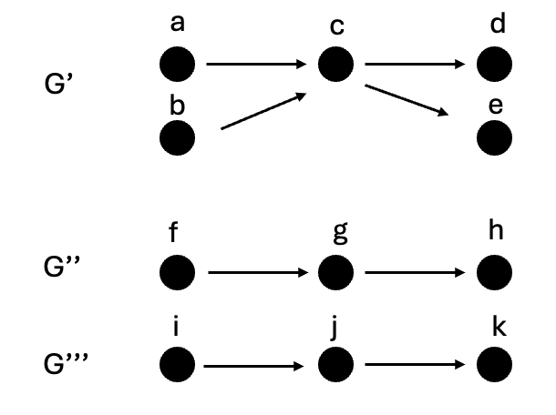
For example, the dag where is connected, but the dag where is not connected.
Definition 9.
Given a dag , its underlying undirected graph is partitioned into connected components. Each component is a connected undirected graph , for some subgraph (see example in Appendix. A.3) of . is termed a component of . A cluster of is a subgraph of that consists of one or more components.
Lemma 2.
Let be a dag and . Then the number of components in is either unchanged or increased by one.
This follows from the definitions, and its proof is omitted. Recall that, according to Theorem 1, in each component of a legal dag there is a path from a vertex in to a vertex in . However, by duplicating an edge, this property can be violated (for example, if the dag contains only one edge , its duplicated graph is not acceptable.) We will use only duplications, defined as follows:
Definition 10.
Let be a dag, and . Then the duplicated graph is if each of its components contains a path connecting a vertex and a vertex .
Lemma 3.
Let be a legal dag, and . Then
-
•
if is an input edge then is not acceptable.
-
•
if is an output edge then is not acceptable.
Proof.
It is clear that in either case, one of the resulting subgraphs does not contain an original input vertex or an original output vertex, thus the resulting dag is not acceptable. ∎
6 Graph Duplication
Given a legal dag , and integers , , we want to duplicate at most edges, such that the resulting graphs will be partitioned into at most clusters, each with at most inputs and outputs (recall that a cluster has one or more components, see Definition 9). Moreover, we require that each of these clusters will be acceptable. Formally, given a legal dag , we want to find a subset , , such that the resulting graph will contain at most disjoint acceptable subgraphs, each including at most inputs and outputs. Note that input graph is not necessarily connected, meaning that some subset of qubits does not interact with another subset of qubits, so one can simulate them separately. Formalized as a decision problem, we ask whether there is a solution to the following problem:
Definition 11.
The Graph Duplication problem .
Input: A legal dag , integers and .
Question: Does there exist , , such that all the components of are acceptable, and can be partitioned into clusters , , satisfying for every ?
7 The complexity of the GD problem
7.1 Overview
This section classifies the computational complexity of the GD problem under different restrictions on the input graph and on the cut budget . First, we show that GD can be decided in polynomial time when is a connected legal dag and is constant. This holds even in the case where the input graph has a constant number of connected components (Theorem 2). Second, GD becomes NP-complete in all other cases; namely, when the number of components is not bounded or the number of duplications (cuts) is not bounded. The NP-completeness proof proceeds through a sequence of reductions: it is shown first for forests and (Theorem 3) and then for any constant (Theorem 4). The same two cases are then shown to be NP-complete also in 2-legal forests (Theorems 5 and 6). Last we show the problem is NP-complete for 2-legal trees and (Theorem 7). In our analysis, we use a reduction from the 3-partition NP-complete problem [20], which is explicitly defined in Appendix C. The main focus of the problem will be on any general legal dag, and in particular on 2-legal dags.
7.2 Connected , constant
Theorem 2.
Problem can be solved in polynomial time for a connected dag , for any constant . This holds even in the case where the input graph is composed of a constant number of connected components.
Proof.
Given a dag , we first list all possible subsets of at most edges; this can be done in time . Then, for each of these subsets , we consider the dag . We first determine its components; this can be done in a time . According to Lemma 2, the number of components is at most . We then examine all partitions of these components into at most clusters. But the number of clusters is clearly bounded by . So we have to examine all possible partitions of these components into at most clusters. The number of these cases is . Each such cluster is then checked in order to determine whether it is acceptable. This is done in time . We have thus established a polynomial time solution to problem . The extension for the case where is composed of a constant number of components is straightforward. ∎
7.3 Forest ,
Theorem 3.
Problem Graph duplication is NP-complete for , even when is a forest dag.
Proof.
We show a polynomial time reduction from the 3-partition problem to .

Given an instance of 3-partition - that is, a set of positive integers , , such that for every - we define the following instance of . The graph is . The set of vertices is , where and , for . The set of edges is . (See Fig 4.)
We set and . Since , no edge was duplicated, so the resulting graph is clearly acceptable. In addition, the reduction can be done in time , and is thus polynomial in the input size.
We have to show that there is a solution to the given instance of 3-partition iff there is a solution to the problem .
Assume there is a solution to the 3-partition problem with input . We show that in this case there is a solution to ; that is, a solution where we do not need to duplicate any edge. For each of the triples in the solution - that is and - the subgraph of composed of , together with all edges, contains exactly inputs and outputs. Clearly, there are exactly paths connecting an original input vertex to an original output vertex. This partitions to exactly parts as required.
Conversely, if there is a solution to then must be partitioned into subgraphs, containing the basic subgraphs with inputs, such that . This establishes a solution to the given instance of the 3-partition problem. ∎
7.4 Forest , constant
Theorem 4.
Problem Graph duplication is NP-complete for any constant , even when is a forest dag.
7.5 Forest , 2-legal dags,
Our motivation for the specific proof of the 2-legal dag defined in Condition is that any multi-qubit gate can be decomposed into a sequence of one- and two-qubit gates, involving at most two-qubit interactions [14].
We now extend this NP-completeness result to 2-legal dags, that is, dags that satisfy Condition 3’.
Theorem 5.
Problem Graph duplication is NP-complete for 2-legal dags , for , even when is a forest dag.
The proof appears in Appendix B.
7.6 Forest , 2-legal dags constant
Theorem 6.
Problem Graph duplication is NP-complete for 2-legal dags , for any constant , and the underlying undirected graph of is a forest.
The proof is in Appendix B.1.
7.7 2-legal connected dags, non constant
Theorem 7.
Problem Graph duplication is NP-complete for connected legal dags , even in the case where is a 2-legal tree dag.
Note: In this case is not a constant (in the case where is constant the problem can be solved in polynomial time according to Theorem 2).
Proof.
We extend the proof of Theorem 3.
Given an instance of 3-partition, we construct the graph depicted in Fig. 5.
We show that there is a solution to the 3-partition problem iff there is a solution to problem (recall that in this problem we need to duplicate at most edges, and partition to at most parts, each with at most inputs). A crucial point in this reduction is that, though is connected, we do not require that each of these parts will be connected. Assume there is a solution to . Then we can duplicate all the edges . All components containing and (see Fig 5) contain exactly inputs each. The other components can be grouped into triples , according to the solution of the 3-partition problem . Each such component will have inputs, thus this part will have exactly inputs. We have thus established a solution to .
Conversely, assume there is a solution to . It is clear that each of the ’s must be in a separate component. Thus it is clear that all edges must be duplicated. As there are exactly such edges, it follows that no other edge can be duplicated. Each component containing has exactly inputs.
We thus have a total of parts. By Lemma 3 it follows that we have at most parts in the partition. Therefore, the parts containing the ’s must be partitioned into at most parts, each with at most inputs. Note that all elements in each are in the same partition, according to Lemma 3. One component with the as inputs contains inputs.
Since , we have . Thus, the sum of four or more of the ’s is more than B+4. So each of the partitions contains at most three such sets . But, since there are such sets, if any partition has less than 3 then there will be a partition with more than 3, a contradiction. Thus, each partition has exactly 3 such sets . If they correspond to the elements , then , thus .
Summing for all triples, we get that . But, since , it follows that for each of these components . We have thus established a solution to .
Extending the result to the case of 2-legal dags is done by using the technique presented in the proof of Theorems 5 and 6.

∎
8 SMT solver
Motivated by the analysis in [15], we propose in this section an SMT-based solution for the circuit cutting problem taking into account our aforementioned definitions. The SMT solver (Microsoft Z3) was constructed based on our GD problem (Definition 11), where the solver attempts to minimize the number of duplications . If the SMT solver does not find a solution, the program will end without any partition. The SMT formulation provides an exact optimization framework for the encoded GD problem, suitable for modest instance sizes (and relatively small values of ), although worst-case runtime remains exponential. The exact constraints are:
-
•
The set , with each indicating whether vertex is in partition .
-
•
The set , with each indicating whether edge is cut.
-
•
For any and , . In other words, for each , .
-
•
For each partition p: there is a path , where implies that there is a path from to using only vertices and edges in partition .


The proposed SMT solver (see [21]) takes as an input a legal dag, a maximum per-partition qubit budget , and an upper bound on the number of partitions max. The legal dag G contains primary inputs (nodes with no predecessors) and primary outputs (nodes with no successors). Having a legal dag implies that . The solver then tries and stops at the first feasible partitioning. The variables, based on the constraints that were introduced earlier, are: a partition index for each vertex, the number of primary inputs per partition, the number of crossing edges entering each partition, and the total number of duplications, which we minimize. The SMT includes an optional requirement demanding each partition to be fully connected, and for that we use a lightweight breadth-first search (BFS) scaffold to enforce connectivity within each partition (within the “3 partition” reductions this requirement is not necessary). In the program, each vertex is assigned a partition. For each partition the total “qubits” accounted for are the primary inputs plus the incident crossing edges that enter the partition, empty partitions are not allowed. Optionally, one can require that each partition contains at least one and of the same qubit. When requiring each partition to be internally connected, the BFS-like scaffold is defined as follows: in each partition, exactly one node is selected as a root, and every other node in the partition is assigned a strictly positive distance from it. For any edge whose endpoints lie in the same partition, the assigned distances differ by at most 1, and every non-root node has an in-partition neighbor at distance one or less. These constraints guarantee that the subgraph induced by each partition is connected.
The first example depicted in Fig. 6(a), is a unitary operation that can be written as a tensor product of local unitaries. The SMT solver visualization is presented in Fig. 6(b), visualized using our Python implementation (NetworkX). The details of the simulation are as follows. We asked the SMT to give at most two clusters with at most 4 qubits in each. The SMT solver solution depicted in Fig. 6(c), where each cluster has a different color. As was implied above, the SMT solver found partitions without duplicating any edge. Now consider the next test case, in which a feasible solution exists only if duplication is allowed. Repeating the same procedure as in the previous example, the entangled circuit shown in Fig. 7(a) is mapped to the graph in Fig. 7(b), and the resulting solution is shown in Fig. 7(c). The duplicated edge is highlighted in yellow.


9 Discussion
We introduced a graph-theoretic abstraction of timelike quantum circuit cutting and used it to define the graph duplication problem GD. We showed that the GD problem can be solved in polynomial time when is constant and has a constant number of connected components. Then we showed that the GD problem becomes NP-complete in all other cases; namely, when the number of components is not bounded or the number of duplications (cuts) is not bounded. We also presented an SMT formulation aligned with the GD constraints. The SMT solver is intended as a practical optimization tool for moderate-size instances, not as a polynomial-time algorithm for the general problem: like other exact combinatorial solvers, it can still exhibit exponential worst-case runtime. Interesting questions for future research could be to characterize intermediate regimes in which grows with the instance size, for example , and to compare the present abstraction directly with hardware-aware circuit-cutting heuristics used in existing toolchains.
Acknowledgements
This work was supported by the European Union’s Horizon Europe research and innovation programme under grant agreement No. 101178170, by the Israel Science Foundation under grant agreement No. 2208/24 and by the Israeli Council for Higher Education through “QERNEL” and the “Interdisciplinary Center for the Theory of Quantum Computing”.
References
- [1] J. Preskill, “Quantum computing in the nisq era and beyond,” Quantum, vol. 2, p. 79, 2018.
- [2] K. Fukui and S. Takeda, “Building a large-scale quantum computer with continuous-variable optical technologies,” Journal of Physics B: Atomic, Molecular and Optical Physics, vol. 55, no. 1, p. 012001, 2022.
- [3] C. D. Bruzewicz, J. Chiaverini, R. McConnell, and J. M. Sage, “Trapped-ion quantum computing: Progress and challenges,” Applied Physics Reviews, vol. 6, no. 2, 2019.
- [4] Y. Kim et al., “Evidence for the utility of quantum computing before fault tolerance,” Nature, vol. 618, pp. 500–505, 2023.
- [5] K. Bharti et al., “Noisy intermediate-scale quantum algorithms,” Reviews of Modern Physics, vol. 94, p. 015004, 2022.
- [6] T. Peng, A. W. Harrow, M. Ozols, and X. Wu, “Simulating large quantum circuits on a small quantum computer,” Physical Review Letters, vol. 125, no. 15, p. 150504, 2020.
- [7] S. Bravyi, G. Smith, and J. A. Smolin, “Trading classical and quantum computational resources,” Physical Review X, vol. 6, no. 2, p. 021043, 2016.
- [8] A. W. Harrow and A. Lowe, “Optimal quantum circuit cuts with application to clustered hamiltonian simulation,” PRX Quantum, vol. 6, p. 010316, 2025.
- [9] C. Piveteau and D. Sutter, “Circuit knitting with classical communication,” IEEE Transactions on Information Theory, vol. 70, no. 4, pp. 2734–2745, 2024.
- [10] L. Schmitt, C. Piveteau, and D. Sutter, “Cutting circuits with multiple two‑qubit unitaries,” Quantum, vol. 9, p. 1634, 2025.
- [11] C. Piveteau, L. Schmitt, and D. Sutter, “Circuit cutting with classical side information,” Physical Review Research, vol. 7, p. 033063, 2025.
- [12] C. Ufrecht, M. Periyasamy, S. Rietsch, D. D. Scherer, A. Plinge, and C. Mutschler, “Cutting multi-control quantum gates with zx calculus,” Quantum, vol. 7, p. 1147, 2023.
- [13] J. Biamonte and V. Bergholm, “Tensor networks in a nutshell,” arXiv preprint arXiv:1708.00006, 2017.
- [14] A. Barenco, C. H. Bennett, R. Cleve, D. P. DiVincenzo, N. Margolus, P. Shor, T. Sleator, J. A. Smolin, and H. Weinfurter, “Elementary gates for quantum computation,” Physical Review A, vol. 52, no. 5, p. 3457, 1995.
- [15] S. Brandhofer, I. Polian, and K. Krsulich, “Optimal partitioning of quantum circuits using gate cuts and wire cuts,” IEEE Transactions on Quantum Engineering, 2023.
- [16] J. H. Selby, A process theoretic triptych. PhD thesis, PhD thesis, PhD thesis, Imperial College London, 2017.
- [17] J. Biamonte, “Lectures on quantum tensor networks,” arXiv preprint arXiv:1912.10049, 2019.
- [18] J. C. Bridgeman and C. T. Chubb, “Hand-waving and interpretive dance: an introductory course on tensor networks,” Journal of physics A: Mathematical and theoretical, vol. 50, no. 22, p. 223001, 2017.
- [19] H.-Y. Huang, R. Kueng, and J. Preskill, “Predicting many properties of a quantum system from very few measurements,” Nature Physics, vol. 16, no. 10, pp. 1050–1057, 2020.
- [20] M. R. Garey and D. S. Johnson, “Complexity results for multiprocessor scheduling under resource constraints,” SIAM Journal on Computing, vol. 4, no. 4, pp. 397–411, 1975.
- [21] E. Zahavi and Y. Idan, “Quantum split SMT.” https://github.com/YuvalIdan9/circuit_cutting.git, 2024.
- [22] M. R. Garey and D. S. Johnson, Computers and Intractability, vol. 29. W.H. Freeman, New York, 2002.
Appendix A Proof extensions
A.1 Proof of Theorem 1 (a)
Proof.
In any directed graph Hence
Since the sums on both sides of the equation are equal by Condition 3 above, we have
Since by the definition of inputs and outputs, we have
By Conditions 1 and 2 above, the term on the left side is equal exactly to , since each vertex in contributes exactly to the sum, while the term on the right side is equal exactly to , since each vertex in contributes exactly to the sum. Hence . ∎
A.2 Proof of Theorem 1 (b)
Proof.
The proof is by induction on .
Base: . In this case ,. We follow a path starting at . Whenever the path reaches a new vertex , there is always another edge outgoing (due to Condition 3). Since the graph is finite, and since we never enter a previously visited vertex (since is a dag), this procedure must terminate at . Thus, we established a path from to .
Induction step: We show that if the claim holds for then it holds for , for every . Let be a legal dag in which . Take any vertex . Applying the same algorithm as above, we start at , and continue along edges until we end at a vertex . We now delete the edges of this path from , and get a new graph , in which . It is clear that after removing the path from the dag the resulting graph is a dag. Moreover, it is a legal dag, since: (1) we deleted one input vertex and one output vertex, (2) in all other vertices along the path the in-degree and out-degree were decreased by one, thus maintaining Condition 3, (3) no new input or output vertex were created, and (4) the in and out degrees of all vertices which are not on this path remain unchanged. By the induction hypothesis, there are edge-disjoint paths connecting an input vertex and an output vertex. ∎
A.3 Definition 9 - Example
The dag G contains three components . is a cluster that contains one component, and is a cluster that contains two components. Fig. 8 illustrates these components.
A.4 Proof of Theorem 4
The proof is an extension of that of Theorem 3. Given an instance of 3-partition, we construct an instance ; includes the dag (defined in the proof of Theorem 3), to which we add copies of the dag , where , and (see Fig. 9).

Since is constant, this construction is done in polynomial time.
We have to show that there is a solution to the given instance of 3-partition iff there is a solution to the problem .
If there is a solution to then by duplicating all the edges () we get a partition into exactly subgraphs, each with exactly inputs. Conversely, assume we are given a solution to . The key point is that, according to Lemma 3, the only edges that can be duplicated in are the edges (see Fig. 9). Moreover, since each of the dags contains more than inputs , each of these edges must be duplicated – resulting in partitioning of into two dags with exactly inputs in each part – in order to get a solution that satisfies the constraints. Hence, all of these edges must be duplicated. Thus, we get new subgraphs, and thus the remaining graph must have exactly parts, each with exactly inputs, which results in a solution to the instance of the 3-partition problem.
Appendix B Proof of Theorem 5
We use the same reduction as in the proof of Theorem 3, with a slight modification: Each vertex satisfying , is replaced by a subgraph. For example, if then we replace it by the subgraph shown in Fig. 10. The rest of the proof follows the same line.
B.1 Proof of Theorem 6
This is an extension of the proof of Theorem 4, where for each internal vertex with is replaced by the subgraph depicted in Fig. 10. The rest of the details follow the same line.

Appendix C The 3-partition NP-complete problem
3-partition. For our discussion, we refer to the book [22]. We first use the following problem, known to be NP-complete [20]:
Problem 1 (3-partition problem).
: A set of positive integers and a positive integer bound , such that for every , and such that .
: Can be partitioned into disjoint sets such that for every ? (note that each must therefore contain exactly three elements from ).