Enhanced Reconstruction of Sub-GeV Neutrinos Charged Current Interactions in LArTPC
Abstract
This paper presents a comprehensive study of the reconstruction of sub-GeV neutrino charged-current interactions within a Liquid Argon Time Projection Chamber (LArTPC). We demonstrate that traditional charge-based calorimetry is fundamentally limited at sub-GeV scales by significant fluctuations in recombination and missing hadronic energy. We show that energy reconstruction using energy deposited as scintillation light () partially benefits from the self-compensating light effect. At neutrino energies above 400 MeV, the light-only reconstruction still outperforms charge-only methods that can separate EM and hadronic objects. The performance of the two remains comparable below 300 MeV. Using the energy-deposit information from both detector signals, we demonstrate at least 70% efficiency can be achieved in tagging electron neutrinos and antineutrinos, respectively. By using a proximity-based algorithm coupled with a geometric lepton-exclusion cone, we also demonstrate the ability to isolate neutron-induced energy depositions from background. This enables an improvement of sub-GeV direction reconstruction by about 20 degrees for antineutrinos. This study provides new insights into how to enhance the physics reach of future LArTPC atmospheric neutrino analyses.
I Introduction
Since the discovery of neutrino oscillation [17, 9, 10], massive progress has been made in studying atmospheric neutrinos in current-generation experiments such as Super-Kamiokande [11, 12, 2, 26]. Recent efforts culminate in their use to extract the neutrino mass ordering and the leptonic CP-violating (CPV) phase when jointly analyzed with beam neutrino data from T2K [3]. Sub-GeV atmospheric neutrinos are crucial for probing the CPV phase [20]. However, there has been difficulty reconstructing their direction, energy, and charge, which affects the calculation and simulation of the neutrino oscillation probability and weakens the physics sensitivity.
Next-generation neutrino experiments, such as DUNE, will continue to use atmospheric neutrinos to probe the leptonic mixing sector. Once DUNE turns on its far detector at the end of this decade, each 17-kt module will collect hundreds of atmospheric neutrinos [4]. The LArTPC detector technology at DUNE offers new possibilities in the sub-GeV neutrino reconstruction. Previous studies have reported GeV and MeV neutrino reconstruction using charge and light signals in LAr [22, 25], while the sub-GeV energy range study is missing. Meanwhile, DUNE recently reported the capabilities in reconstructing atmospheric neutrinos in its horizontal drift module [1]. The report indicates that the resolution of both neutrino direction and energy reconstruction is significantly improved when incorporating more than just the lepton information. Most importantly, neutral particles such as neutrons constitute a significant part of the missing energy (or momentum) in neutrino interactions. Neutron identification and energy reconstruction via neutron-induced secondary particles are implemented in other detector technologies [18]. It is timely to study more possibilities of sub-GeV neutrino reconstruction in an LArTPC. In this work, we explore ways to improve sub-GeV neutrino reconstruction by leveraging information that has not been extensively studied before, such as the light detection system and neutron energy deposition.
The paper is structured as follows: Section II describes the simulation sample used in this paper. The energy reconstruction performance using both the charge and light detector signals is discussed in Section III. The charge discrimination between neutrinos and antineutrinos is further discussed in Section IV. Section V details the reconstruction of the direction of sub-GeV neutrinos using neutron energy deposits. The complementarity of this work to a recent work in Ref. [21] is discussed in Section VI. The final summary is presented in Section VII.
II Simulation
In this study, charged-current -Ar interactions are simulated for each neutrino flavor (, , , ), using the AR23_20i tune [14] of the GENIE v3.04.00 neutrino event generator, in the sub-GeV range i.e. with incident neutrinos of energies ranging from 100 MeV (200 MeV) to 1000 MeV for and ( and ), in 100 MeV increments. 1000 interactions were simulated per flavor per incident neutrino energy. The edep-sim software package, interfacing with GEANT4 v10.6.p01 – same as the setup used in Ref. [22, 25] – is used to model the propagation and energy deposition of all subsequent primary and secondary particles in an infinite liquid argon volume.
III Sub-GeV Neutrino Energy Reconstruction
Previous simulation studies have shown that light calorimetry in a LArTPC can play a unique role in neutrino energy reconstruction in multi-GeV [22] and tens of MeV [25] energy ranges. This study seeks to fill the gap in the sub-GeV energy regime. The goal is to study the performance of various neutrino energy reconstruction methods similar to those presented in Ref. [22] based on the simulated charge and light signals, with particular interest in assessing the benefits of utilizing the light signal, which will become more enhanced in upcoming LArTPC neutrino experiments such as DUNE [7].
We begin in Section III.1 with a discussion of energy deposition processes for sub-GeV neutrinos, highlighting the differences relative to the multi-GeV regime. We then review the energy reconstruction methods and show their performance in Section III.2. After these, we will interpret the results and comment on differences to the multi-GeV neutrino case in Section III.3.
III.1 Sub-GeV neutrino energy deposition in LAr
We adopt the same definition as Ref. [22] for the total available energy, , which includes the kinematic energy of protons and neutrons, and the total energy of electrons, pions, muons, and gammas. Smearing effects between and , which fluctuate from event to event, contribute to a spread in the distribution. The AR23_20i tune [14] used in this work models energy loss from the nucleon removal, which varies with the nucleon momentum. More significantly, some energy is gained or lost during final-state interactions (FSI). The hadrons produced in the initial neutrino interaction interact with other nucleons in the struck 40Ar nucleus, which could produce additional nucleons in the final state as well as occasional re-absorption of some primary hadrons. FSI is less pronounced in the multi-GeV neutrino interactions, but is crucial for sub-GeV neutrinos.
The dotted light-blue histogram and the blue histogram in Fig. 1 show the distribution of the total available energy before and after the FSI, respectively, for a 0.4 GeV sample. As can be seen, many events (36% of the sample) do not see any change in before and after the FSI. These events also have the same list of particles at the primary vertex before and after the FSI, so it is safe to assume no FSI happens in these events. However, according to the model, for the majority of events, FSI increases (52% of events in the sample) rather than decreasing it (12%). While the fraction of events that see no FSI appears to remain approximately 30% across the sub-GeV range, the fraction of events where FSI raises decreases from 70% at MeV to 50% at MeV. Since the exact relationship between the simulated and the true is highly model-dependent, we will focus on estimating from the simulated detector signals, which is a reasonable approximation for the true .

After FSI, all outgoing particles deposit their energy in LAr by either ionization or excitation interactions with 40Ar atoms. However, not all is deposited. The orange histogram in Fig. 1 shows the distribution of the total deposited energy, , for the 0.4 GeV sample. The distribution has a much longer tail toward lower energies due to varying amounts of missing energy. The most prominent sources of missing energy are from neutrons and charged pions. Neutrons, being electrically neutral, cannot ionize or excite nearby 40Ar atoms to deposit their energy. Instead, depending on their kinetic energy, they interact with 40Ar nuclei through elastic and inelastic scattering, transferring part of their energy to recoiling nuclei or producing secondary particles, such as de-excitation rays and additional nucleons. Inelastic scattering also results in some of the neutron’s kinetic energy being lost to the binding energies required to break up the nucleus and release secondary hadronic particles. The amount of energy lost in nuclear breakup can vary significantly from event to event. At higher energies, neutrons can also induce spallation and other nuclear reactions. While charged pions can continuously deposit energy in LAr, they decay with some carried away by neutrinos. Figure 2 shows that events with neutrons and pions are mostly responsible for the tail in the distribution we attributed to missing energy.

Particles deposit energy in the LAr by ionizing or exciting 40Ar atoms. In this simplified model, a constant fraction of the deposited energy is assumed to produce ionization electrons, while the remaining fraction is converted into scintillation photons. The recombination of ionization electrons and argon ions results in some electrons essentially being exchanged for scintillation photons. As such, the actual fraction of quanta that end up as ionization electrons is , where is the charge recombination factor and depends on the electric field of the LArTPC and the of the specific particle. is calculated in the simulation using the Birks’ Model as implemented in Ref. [22]. Taking this into account, one can break up the total deposited energy as a sum of two components: the energy in ionization electrons, i.e., charge,
| (1) |
and the energy in scintillation photons, i.e., light,
| (2) |

Charge () and light () are the detector signals that are used to reconstruct the incident neutrino energy. The and distributions are shown in the red and purple histograms, respectively, in Fig. 3. Here, we also consider an optimistic 75 keV charge detection threshold to reflect that detector readout noise sets a minimum limit on the amount of charge that can be reconstructed. The distribution after applying this threshold ( or interchangeably ) is shown in the green histogram of Fig. 3. While the distribution of maintains roughly the same shape as , its peak is less sharp due to the recombination effect. For the light collection, we have assumed a uniform photon-collection efficiency of 0.83%, corresponding to an average light yield of 180 photoelectrons per MeV for a MIP. The expected number of detected photons and the final detected energy deposited in light follow the same treatment presented in Ref. [25, 22]. The distribution is less smeared out and more symmetric than the distribution. The reasons for this will be addressed in Section III.2 below.
At this point, it is important to summarize the differences between the energy share profiles of sub-GeV and multi-GeV CC events. In Ref. [22], it was found that only 10.4% of the in 3 GeV events is deposited by protons and their descendants. By contrast, this fraction increases to 24.9% in sub-GeV events (Fig. 4). This fraction remains stable in the 23%-26% range across all 200-1000 MeV samples. This increase is compensated for by having a smaller fraction of deposited in pions (2.7% versus 9.8%). Below MeV, essentially no pions are created. There is a slight decrease in the fraction deposited by the EM component (59.6% versus 64.5%). The fraction of missing energy is also slightly less in the sub-GeV regime (6.6% on average instead of 8.0%). Also, essentially no other heavier particles (which made up 1.3% of the 3 GeV ) are created.

In addition to contributing a larger share of the deposited energy, the final-state protons in the sub-GeV regime also have a smaller average percentage of missing energy than the 3 GeV events (4.5% versus 11.8%). Primary neutrons behave similarly in both energy regimes, with 38% missing energy for sub-GeV events and 36% for 3 GeV. The fraction of missing energy increased for primary charged pions (34.5% versus 24.7%). This is expected since pions are created with smaller in sub-GeV neutrino events. However, primary pions are only in of sub-GeV events. The percentage of missing energy in the EM component is consistently negligible across energy regimes (0.04%).
Overall, the difference setting sub-GeV events apart from the multi-GeV case is the larger role of the primary protons in the deposited energy: a greater fraction of the events’ is apportioned to protons, and most of the proton kinetic energy is deposited. This has significant implications for the quality of energy reconstruction achievable in this regime, because the charge recombination factor for low-energy protons is much lower than that for high-energy MIP protons and depends on their .
III.2 Methods of energy reconstruction
As discussed above, only a fraction of a particle’s is actually visible to a calorimeter in the form of or . This fraction is defined as the calorimetric response as in Ref. [22],
| (3) |
where is the energy deposited as charge () or light () signals in the simulation. Naturally, if we knew for a neutrino event, we could divide out the recorded visible energy by to get the true available energy. However, the calorimetric response from individual outgoing particles can fluctuate significantly. The charge and light calorimetric responses are plotted in Fig. 5 for different groups of particles in sub-GeV neutrino events. We have previously noted that sub-GeV events have a larger fraction of their deposited energy in protons, meaning that lower-energy protons constitute a larger fraction of the hadronic component in the sub-GeV regime than in the multi-GeV case. We also note that the charge recombination factor for protons decreases steeply with the initial proton kinetic energy below 200 MeV (cf. Figs. 9 and 10). Thus, on average, the charge calorimetric response is lower and the light calorimetric response correspondingly higher for the hadronic component of sub-GeV events than for that of multi-GeV events. By contrast, the EM-component calorimetric responses for sub-GeV and multi-GeV events are essentially identical.

From Fig. 5, we extract the peak calorimetric response in each distribution as scaling factors that would, when divided by, approximately scale the peak in the visible energy signal – whether that be , , or – to the peak in the distribution of for a sample of events. Below, we consider five major methods of energy reconstruction. Most of them follow Ref. [22], except we consider one more method of combining charge and light signals (Q+L):
-
•
L1: a neutrino energy reconstruction based solely on light signals. We divide out the energy deposited as light by the peak overall light calorimetric response found from the simulation sample,
(4) -
•
Q1: a neutrino energy reconstruction based solely on charge signals. Similarly, we divide out the energy deposited as charge by the peak overall charge calorimetric response ,
(5) -
•
Q+L: a neutrino energy reconstruction based on the summed energy deposited in charge and light. We divide out the sum of the energies deposited as charge and light signals by the peak overall combined calorimetric response ,
(6) -
•
Q2: a neutrino energy reconstruction based solely on charge signals with the assumption that the charge signals from the hadronic and EM components can be separated in the detector. We will divide out the energy in charge depositions originating from EM primary particles only – – by the peak EM-component charge calorimetric response to reconstruct the EM-component available energy, and add it to the energy in charge depositions originating from hadronic particles only – – divided by the peak hadronic-component charge calorimetric response ,
(7) -
•
Q3: a neutrino energy reconstruction based solely on charge signals with the assumption that the track objects can be separated from blip-like objects, and we can also differentiate blip-like objects between those from EM primary particles and hadronic primary particles. This is the ideal case, but it is challenging to realize in experiments today. We assert that energy for all particles whose tracks are longer than 2 cm can be faithfully reconstructed. Then, the available energy can be reconstructed by dividing out the energies in the EM- and hadronic-component dot-like charge depositions and respectively by the respective peak calorimetric responses and adding them together with the total measured energy deposited by tracks:
(8)
We apply all methods to each sub-GeV neutrino sample and obtain a distribution of the reconstructed available energy from each method. One example is shown in Fig. 6 for the 0.4 GeV sample. We then calculate the resolution and relative bias achieved by each method, where resolution is defined as the RMS of the distribution divided by the mean reconstructed energy and the relative bias is defined as i.e. the relative difference between the mean reconstructed energy and the true incident energy. The resolution and relative biases of the five methods are plotted as a function of in Fig. 7.


III.3 Discussion of sub-GeV energy reconstruction performance
All five methods ultimately attempt to reconstruct the total available energy of the event. It stands to reason that the best achievable performance of the energy reconstruction methods described above would be the resolutions of the simulated true itself. This is shown in Fig. 8. It shows that the resolution of the true available energy improves monotonically with . The L1 and Q3 reconstruction results in Fig. 7 nicely preserve this trend. However, at higher , the resolutions of Q1 and Q2 diverge significantly from this trend. Below, we discuss the performance of each of the five reconstruction methods.

Q1
To understand why Q1 has degraded resolution at higher in Fig. 7, we can look at the charge calorimetric response for different kinds of primary particles as a function of their available energy, as shown in Fig. 9. We observe first that almost all possible values of hadronic particles () are well below the possible values of the electron (which are tightly constrained around 0.55). This is because of the high recombination effect for low-energy protons due to their large dE/dx (suppressing their in favor of ), and larger amounts of missing energy for neutrons and pions (diminishing both their and ). Because of this, the true overall will fluctuate significantly from event to event with different splits of between the components. This limits the resolution achievable when we uniformly divide all events’ total by just the peak of the distribution, as done in Q1.

As we go to higher , a wider range of available energies becomes possible for the primary particles. Note that, as can be seen in Fig. 9, at lower energies, the values for protons and neutrons tend to be in a similar low range. Therefore, whether or not an event even has a primary neutron and how the is distributed between protons and neutrons makes little difference to the overall . However, as we move to higher , higher-energy primary protons and neutrons are produced. In this case, the distributions begin to diverge, with primary neutrons on average having significantly smaller than primary protons. This causes the event-to-event fluctuation in the overall to increase with rising , to the extent that the Q1 reconstruction fails to reconstruct well for higher in Fig. 7.
L1
The above discussion on Q1 begs the question of why the L1 method does appear to faithfully reconstruct the at higher , given its resolution continues to monotonically decrease with . Again, we can understand the behavior of this method better using the scatter plot of the light calorimetric response values for different primary particles in Fig. 10. Here, we see that unlike the charge calorimetric responses, the average electron and the average hadronic particle’s are much closer to each other – even for these sub-GeV events, there is to some extent self-compensation in light calorimetry [22] between the calorimetric responses of the EM and hadronic components. This is because, unlike in the case of charge, the stronger recombination for primary protons increases their above that of electrons, while the greater missing energy for neutrons and pions still lowers their below that of electrons. Consequently, the fluctuation in the overall due to varying partitions of the total available energy into the EM and hadronic components is greatly reduced, compared to charge.

This is consistent with how, in Fig. 5, the overall peak is close to both the EM- and hadronic-component peaks, while the overall peak is far from the hadronic-component peak. The self-compensation in does not reach the extent seen in multi-GeV events, where the EM- and hadronic- essentially peak at the same value. It is nevertheless sufficient in the sub-GeV case that, even using only the light signal, the relatively simple L1 method achieves performance comparable to that of the more complex Q3 method based on charge signals.
Additionally, at higher energies, the values of the different hadronic particles converge toward that of the electron, meaning the light self-compensation effect strengthens with increasing energy (consistent with its prevalence in the multi-GeV case [22]). Consequently, the presence of varying hadronic primary particles, and the energy partition among them, causes less event-to-event fluctuation in the overall at higher energies. It therefore makes sense that L1 continues to reconstruct well and thus continues to improve in resolution at higher in Fig. 7.
The worse resolution of L1 compared to Q1 at the lowest is also expected: the values of the lowest-energy primary hadronic particles span the entire range from 0 to 1, whereas the corresponding values do not.
Q+L
Ref. [22] also suggested that Q+L does not offer any significant advantage over Q1 for multi-GeV neutrino events because the Q+L reconstructed energy distribution inherits the missing energy long tail from Q1. However, as seen in Fig. 7, Q+L performs well across the sub-GeV range, achieving comparable resolutions to L1 and Q3 even at the higher . Given that, in the sub-GeV events, the smearing due to recombination is a much more pronounced source of variance in Q1, adding and together to eliminate this smearing naturally yields a greater benefit. In addition, we found in Section III.1 that sub-GeV events overall have less missing energy on average: more of the available energy gets allocated to protons – which tend to deposit close to 100% of their energy – as opposed to pions (a large source of missing energy). It is therefore reasonable that Q+L performs better in the sub-GeV than the multi-GeV regime.
Q2 and Q3
The crux of the reason why Q2 fails to reconstruct well at high (and thus has a worsening resolution beyond MeV) but Q3 does not is the fact that proton tracks in sub-GeV events have a large variation in their values. Despite the fact that almost all proton tracks consistently deposit essentially 100% of their available energy into the LAr, proton tracks of different initial kinetic energies have significantly different fractions of their deposited energy in charge () as opposed to light () due to differing amounts of recombination (Figs. 11 and 9). The average of a proton track increases from close to 0 (all deposit energy goes into light) at kinetic energies near 0 MeV to approaching around 0.55 at the highest achieved kinetic energies, with the relationship becoming increasingly steep at lower kinetic energies.

At higher , each primary proton created in an event has a wider range of permissible available energies to start with – from 0 to a little less than – and so each primary proton has a wider range of possible values. This makes scaling the hadronic-component values obtained across many events by any single factor increasingly ineffective as increases.
Q3 does not have this issue, because if proton tracks can be identified and their dE/dx measured, we can exactly account for the amount of recombination that occurs for each proton track to reliably reconstruct its total – and consequently also its , since protons deposit almost 100% of their energy. We can test this reasoning with a modified Q3 reconstruction method in which we assume we are unable to separate out tracks associated with primary protons; instead, we include the charge-deposited energy () of all primary protons and their descendants in the term, to be scaled up by a single factor. As seen in Fig. 12, this modification to Q3 performs essentially identically to Q2, with degraded resolution at higher .
We can also compare the sub-GeV reconstruction result with the results for multi-GeV events in Ref. [22]. The resolutions we obtained for L1, Q1, and Q3 at 500 MeV and 1000 MeV are generally consistent with Fig. 10 in Ref. [22]. However, the resolutions we obtained for Q2 at these two neutrino energies are around 5 percentage points higher (i.e., worse). This is explained by the fact that the scale factor we have employed to scale the hadronic component deposited energy in charge is significantly smaller than the corresponding factor used in the multi-GeV study for reasons discussed in Section III.2.

IV Sub-GeV Neutrino and Antineutrino Separation
As outlined above, the ability to distinguish neutrino events from antineutrino events is crucial for measuring the CP phase in neutrino oscillations. For charged-current interactions, and events differ in the sign of the charge of the final state lepton. Previous studies [19] have suggested that and could be distinguished in an LArTPC by their tendency to capture on Ar nuclei, which does not occur for and . However, no such asymmetry exists between and for - separation. And the rarity of charged pions in sub-GeV events limits the effectiveness of that avenue.
Another prominent difference between and CC interactions is that for charge to be conserved, () events will almost always involve at least one primary proton (neutron), particularly in the sub-GeV regime where most events are quasi-elastic scattering events. One potential approach for - separation could therefore be via final-state topologies, including the use of isolated energy deposits from neutrons [21]. However, this is somewhat complicated by final-state interactions, which are highly model-dependent.
With enhancements in light-calorimetry capabilities in LArTPC, and themselves become sufficiently distinct between and . Below, we discuss in detail some of the calorimetric features that could be used for charge separation.
IV.1 Calorimetric Differences between Electron Neutrino and Antineutrino Events in LAr

As shown in Fig. 13, the fraction of deposited by primary protons and their descendants across all sub-GeV events is about a quarter of that for sub-GeV events (6% versus 25%). The difference is made up in sub-GeV events by roughly double the fraction of deposited by neutrons and their descendants (11.8% versus 6.1%), a larger fraction deposited in the EM component (68.7% versus 59.6%), and, as expected, slightly more missing energy (8.6% versus 6.6%).
Recall that protons have larger and consequently smaller – particularly at lower energy – as compared to neutrons and (which consistently have in this energy regime), which means a proton depositing the same total amount of energy as a neutron or would result in less additional but more . So, the fact that a comparatively much larger share of the is deposited by protons suggests that a event of similar to an event will have substantially greater . This is in fact what we observe when we plot against for the simulated and event samples with from 100 MeV to 1000 MeV (Fig. 14). The and events appear to be linearly separable. This motivates the idea that a relatively simple machine-learning model trained on these calorimetric features could classify events as or with reasonable accuracy.


Another calorimetric difference of interest identified between and events is an apparent asymmetry in the impact of the charge threshold. Specifically, it was observed that, when the threshold is increased from 75 keV to 500 keV in the simulation for individual -deposits, the relative drop in total was on average larger for events than events. This is well illustrated in Fig. 15 where a significant separation is visible between the distribution of in and events, with the majority of events with being and the majority below being . The reasons for this are elucidated in Appendix A, though, in short, this is another reflection of the fact that protons have a significantly larger on-average share of in events than in events.
Practically, the charge threshold is bounded below by hardware limits, though it could always be artificially raised during event reconstruction. Meaning that if the charge-readout hardware supports a 75 keV charge threshold, performing the - comparison for real events would be feasible.
IV.2 Multivariate Analysis Using Calorimetric Information for Electron Neutrino and Antineutrino Separation
We have identified a few calorimetric variables above for which we qualitatively observe some separation between and events. Now, we employ machine-learning (ML) classification algorithms to quantitatively assess the classification performance achievable with a model based on these variables and to better understand how much discriminative power each variable provides. We will compare the selection performances of ML models which use only (i.e. only basic charge calorimetry), that use alongside the light-calorimetry information or the alternate-charge-threshold information , and finally models which utilize all three together (, and ).

Since we do not know a priori which specific model architecture best relates the calorimetric variables of interest to the neutrino charge, we test three common models: Logistic Regression (Logit), Support Vector Machine (SVM) with the Radial Basis Function (RBF) kernel, and Adaptive-Boosted Decision Trees (AdaBDT), as implemented in the scikit-learn [24] Python library. All three have hyperparameters that can be freely tuned and generally control the model’s complexity. For SVM and Logit, the hyperparameter is inversely proportional to the strength of the regularization penalty term. RBF SVM also has the hyperparameter, which controls how smooth or jagged the non-linear decision boundary is. The BDT’s complexity is determined by the number of trees in the ensemble and the maximum allowed depth of each individual tree.
To avoid overfitting, we follow a common procedure by splitting the sample into a training set of 16,000 events and an evaluation set of 4,000 events. We ensure that the uniform distribution of and equal frequency of and events are maintained in both.
Next, to tune the hyperparameters, we search over a grid of possible hyperparameter values for each model and, for each combination, compute the average accuracy across a 10-fold stratified cross-validation. That is, we randomly shuffle and split the development dataset into 10 subsets (again maintaining the uniform class and distribution), and for each subset compute the accuracy the model achieves on it upon being trained on the other nine (the accuracy being the fraction of all test-events correctly classified). If, for a given combination of hyperparameters, the model performs well across all 10 randomized train-test splits, we can be reasonably confident that the model’s performance does not depend on patterns in the sample’s noise. Therefore, we select the hyperparameter values that maximize this cross-validated average accuracy. We made sure to expand the search range until none of the best hyperparameters were found to be at the edge of the search grid (except in the 1-feature case with Logit and AdaBDT).
Each model is then re-trained on the entire development set with the optimal hyperparameters, and finally applied to the evaluation dataset.
Results
A clear and comprehensive comparison of the different models across combinations of the calorimetric variables can be achieved by plotting the Receiver Operating Characteristic (ROC) curve for each model, as shown in Fig. 16. The ROC curve plots the true positive rate (TPR), the fraction of actual events labeled correctly as , against the false positive rate (FPR), the fraction of actual events labeled incorrectly as , obtained as the selection threshold is varied across the entire range of scores computed by the model for the evaluation-set events. Note that the TPR and FPR are really the selection efficiency and one minus the selection efficiency, respectively. Also, note that both the and selection purities increase with higher TPR (when FPR is fixed) and decrease with higher FPR (when TPR is fixed). An effective classifier will minimize the FPR for each TPR, i.e., reliably reject even as it selects more (by lowering the selection threshold).
In Fig. 16, we find that for the majority of TPR values, the BDT achieves a smaller FPR than the corresponding Logit model, and the corresponding SVM in turn achieves a smaller FPR than the BDT. Meaning that, in general, the SVM is most capable of exploiting calorimetric variables to separate and . This can also be seen by comparing the areas under the ROC curves (AUC), which steadily increase going from Logit to BDT to SVM. As such, since we are interested in comparing the discrimination power of different sets of features, we restrict our focus to the SVM models.
The ROC curves for the SVM models alone are reproduced in Fig. 17, along with confusion matrices for the models’ predictions at the default selection threshold (Fig. 18).


We see that relying solely on a single charge-calorimetric variable, even at a low charge threshold, cannot provide any significant discrimination power. The ROC curve of the -only SVM model is by far the closest to the diagonal, i.e., to a random-guesser, with an outstandingly low AUC of 0.55 (a random-guesser would have an AUC of 0.50). From the confusion matrix, we find that its classification of events is essentially no better than random guessing, too. However, it does classify events slightly better than a random guess, raising both and purities above 50%.
The addition of the light-calorimetry variable alongside results in an immediate boost in performance, with the AUC jumping to 0.74. Looking at the confusion matrix, the gain would appear to be largely isolated to the events, with the efficiency rising from 57% to 83% while the efficiency only rises to 52%. However, the ROC curve makes it clear that by raising the selection threshold, we could instead isolate the gain to : to keep efficiency at 57% while raising efficiency to roughly 75%.
If in place of we instead used another charge-calorimetry variable taken at a higher charge-threshold , we would still obtain a similar boost in performance, reaching an AUC of 0.76. The confusion matrix at the default cut would imply that the model’s performance is more ’balanced’ than the model: achieving a 76% efficiency while still managing 63% efficiency. Though this is a somewhat unfair comparison: the ROC curves show that, with a higher selection threshold, the model could still reach 70% efficiency at the same 63% efficiency.
One question which naturally arises from the above discussions is: if the separation between and seen in the relationships of and reflects in both cases the events’ differing share of in protons, then is the additional information provided by light-calorimetry redundant with the information provided by charge-calorimetry just with a higher threshold ?
It is true that the model achieves a slightly higher AUC than the (by 0.023). However, inspecting the complete ROC curves reveals the full picture: if the priority is to achieve the highest efficiency or TPR at the cost of poor efficiency and purity, then the model with a sufficiently low selection threshold is superior. Whereas, if the priority is to minimize the FPR – and so maximize the purity and efficiency – at the expense of the efficiency, then the model with a high selection threshold is the better option. Moreover, the ROC curves do in fact intersect, meaning for a certain (non-trivial) choice of two thresholds the two models actually would perform identically well (with an 84% efficiency but essentially-50% efficiency).
Were to be redundant with for charge separation, we would see no significant gain in performance from the model to the model which uses all three: . However this is refuted by the default-threshold confusion matrices: even though the model sees a slightly lower efficiency (72%, down from 76%), the increase in efficiency – from 63% to 75% – is enough that the overall accuracy rises from 69.7% to 73.5% (the highest accuracy achieved among all models tested), and both purities increase as well. In fact, out of all models evaluated, only the SVM using all three calorimetric variables scores above 70% for all four efficiency and purity metrics at the default cut.
The superior performance attainable upon the inclusion of is validated by comparing the full ROC curves. The model’s curve clearly surrounds the other three – for almost any value of TPR, i.e., efficiency (except around 0.3-0.45), it provides better efficiency (lower FPR) and thus purity than the other three feature sets. One sees that by choosing lower selection cuts, one could improve the efficiency above the default-threshold model without any loss of efficiency or vice versa. The model has the highest AUC of 0.80 (0.043 above the model’s).
It is thus clear that, in order to achieve the optimal overall classification performance, all three calorimetric variables – the two charge-threshold values and the light-calorimetry – are necessary.
We have shown that even a model as simple as SVM is able to achieve substantial - classification performance with only three calorimetric variables. Naturally, a practical machine-learning neutrino flavor-reconstruction model would be far more complex and would include a broader array of (less model-dependent) event information, such as track lengths, the number of blips, etc., thereby yielding stronger, more robust classification. Nevertheless, this study emphasizes the benefits of advances in calorimetry capabilities, both in further developing light calorimetry and in lowering the charge threshold to enable the - comparison to be exploited.
V Sub-GeV Neutrino Direction Reconstruction
In addition to neutrino energy reconstruction and charge separation, accurate neutrino direction reconstruction is also crucial for precise measurements of neutrino oscillations using sub-GeV atmospheric neutrinos [20]. The current atmospheric neutrino direction reconstruction typically employs two paradigms: using lepton-only information or using all reconstructed particles [1]. The first method estimates the direction of the incident neutrino solely from the reconstructed primary lepton. Although robust, this ignores the significant momentum contribution of the hadronic system. The second approach attempts to reconstruct the hadronic system but is fundamentally limited by the missing momentum from neutral particles, primarily neutrons. In LArTPCs, neutrons only manifest through sporadic energy deposits [16] or secondary tracks such as protons [6]. This is particularly problematic for antineutrino interactions, where the charged-current process frequently ejects one or more neutrons. Neutrons share up to 44% of the total energy of all outgoing particles, as shown in Fig. 19. In the sub-GeV region, many protons are also not energetic enough to leave a track, so a large fraction of proton activity is missed. These further motivate neutron reconstruction and low-energy hadronic system reconstruction, which is indispensable for neutrino direction reconstruction.
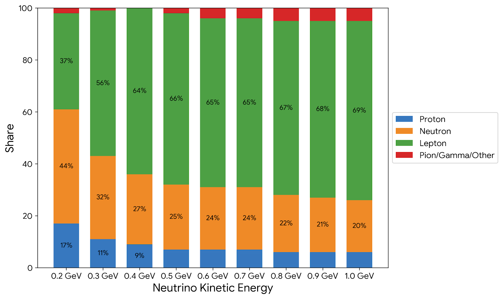
We present a method to reconstruct the neutron momentum vector in LArTPCs. The discussion will focus on neutron direction reconstruction (Section V.1) and neutron momentum amplitude reconstruction (Section V.2). After these, we will evaluate how the sub-GeV neutrino reconstruction performance improves with neutron momentum reconstruction (Section V.3).
V.1 Neutron direction reconstruction
Our neutron direction reconstruction methodology employs a proximity-based algorithm in which the incident direction is defined by the vector from the neutrino interaction vertex to the spatially nearest energy deposition. This approach is predicated on the assumption that the first neutron scattering provides the most accurate representation of the primary neutron direction; subsequent interactions are characterized by isotropic scattering, leading to a random walk that degrades directional information.
Although the chronologically earliest neutron interaction point would provide the optimal direction reconstruction, the limited temporal resolution of isolated, low-energy deposits in current LArTPCs precludes this possibility. Consequently, the spatially nearest neutron deposition to the neutrino interaction vertex serves as a proxy for the earliest neutron interaction. Fig. 20 suggests that this spatial proximity maintains high directional fidelity, as the nearest deposition remains highly correlated with the primary neutron interaction point for a majority of events.

A critical component of this methodology is discriminating neutron-induced isolated energy deposits from competing backgrounds. Notably, primary electrons that propagate as electromagnetic showers frequently produce fragmented energy signatures that topologically mimic neutron-induced hits. We propose a geometric isolation based on a conical veto volume centered at the primary neutrino vertex as shown in Fig. 21. The central axis and longitudinal extent of the cone are determined by the trajectory and range of the primary outgoing lepton, which are reconstructed reliably at this energy range by algorithms used in current LArTPCs [5, 8]. This geometric isolation is designed to suppress lepton-induced backgrounds by excluding the majority of the volume where the lepton deposits its energy.

A successful neutron direction reconstruction is defined when the nearest energy deposition among all depositions outside the conical veto volume is associated with the true primary neutron. There are some failure modes, for example, when the nearest deposition originates from non-neutron backgrounds, and when the primary neutron undergoes its initial interaction within the excluded conical volume. By scanning the cone opening angle , we optimize to maximize the efficiency of picking up the nearest neutron energy deposition outside the veto cone (),
| (9) |
The optimal cone geometry is highly dependent on the lepton flavor and its associated energy deposition profile, as shown in Fig. 22:
-
•
and : In interactions, the resulting consistently undergoes decay-at-rest, producing a Michel electron (). At low energies, this secondary deposition necessitates a wider cone. The optimal exclusion cone narrows as the muon’s kinetic energy increases.
Conversely, for interactions, approximately 75% of in the simulation are captured on the 40Ar nucleus [15]. This nuclear capture suppresses the Michel electron signal, thereby allowing a more constrained exclusion cone than in the antineutrino channel.
-
•
and : The electron or positron typically travels approximately one radiation length ( cm in LAr) before initiating an electromagnetic shower. The transverse profile of this shower is characterized by the Molière radius ( cm) [13]. Because is a property of the medium, the shower width remains relatively constant regardless of energy; thus, the optimal cone angle is largely uncorrelated with the lepton’s kinetic energy as shown in Fig. 22.
Additionally, we apply a detector energy threshold of 0.6 MeV to simplify the treatment of the dominant radiological background in bulk LAr, whose decay produces electrons with a maximum energy of 565 keV. In Appendix B, we demonstrate that the background has a non-negligible impact on the final result, even if the region of interest for finding the neutron’s nearest energy deposit is small. When we lower the energy threshold from 0.6 MeV to 0.3 MeV or 0.1 MeV, the improvement contributed by neutron momentum reconstruction will be diluted in the final reconstruction of the neutrino direction.

Localized energy deposits from low-energy protons also constitute a background for this analysis. We consider a conservative kinetic energy threshold of 70 MeV for a proton to produce a detectable track in LAr; protons with kinetic energies below this threshold are considered blip-like. Because sub-threshold proton energy depositions are tightly clustered around the neutrino interaction vertex, they can be effectively excluded by applying a 5 cm radius spherical spatial cut centered on the neutrino vertex. Crucially, this spherical cut preserves the majority of the primary neutron energy depositions central to this study, as illustrated in Fig. 23.

From the simulation, we also observed that most of the earliest neutron energy deposition is within a 1.5-meter radius from the neutrino vertex. We adopt this region of interest (ROI) for identifying the nearest neutron energy deposition. Using a larger ROI volume would include more noise and affect the reconstruction. We reserve this discussion for the next section where we describe the neutron momentum reconstruction. At the sub-GeV energy range, it is also possible to have multiple neutrons produced as a result of various nuclear effects. Experimentally, it is challenging to resolve these. In these cases, we treat the energy depositions from all neutrons as a single effective low-energy system emanating from the vertex.
To summarize, for the neutron direction analysis, within a ROI sphere of radius 1.5 m and excluding an inner 5-cm radius spherical veto region around the neutrino vertex, all localized, blip-like energy depositions above 600 keV outside the lepton veto cone are considered neutron energy deposit candidates. The vector pointing from the neutrino vertex to the nearest of these candidate depositions is taken as the reconstructed neutron direction. The performance of the neutron direction reconstruction is shown in Fig. 24. The peak around zero shows those events where the earliest neutron energy deposit is, in fact, the nearest energy deposit, and we perfectly reconstruct these events. Deviations from the true neutron direction exist, but the fraction of these events decreases at larger angle deviations and reaches a minimum in the opposite direction of the neutron’s true momentum.

V.2 Neutron momentum amplitude reconstruction
The neutron momentum amplitude reconstruction is based on the relativistic relation between the neutron kinetic energy () and its momentum amplitude ():
| (10) |
The task is to reconstruct the initial neutron kinetic energy () from the energy deposition near the neutrino vertex. The strategy is to sum the candidate neutron energy depositions and find the relation between this quantity and the true neutron kinetic energy. In the simulated sample, about 60% of the neutron energy deposition above the detection threshold of 0.6 MeV falls into a sphere of 1.5 m radius around the neutrino vertex. To start with, we first exclude depositions more than 1.5 m away from the neutrino vertex, and then use cones as defined in the previous section to exclude all track-like energy depositions, including those from muons, pions, and protons with kinetic energy above 70 MeV. The summed candidate neutron energy deposits and the true neutron kinetic energy are plotted in 2-dimensional histograms for four neutrino flavors in Fig. 25.
We divide the plot into three regions and use different binning schemes to record the distribution, ensuring we do not infer a relationship from insufficient statistics. The bin sizes are 15 MeV 15 MeV below 60 MeV of summed energy deposit, 30 MeV 30 MeV for summed energy deposit between 60 MeV and 210 MeV, and 50 MeV 50 MeV when the summed energy deposit is above 210 MeV, respectively. For each summed-deposits bin, we find the most probable initial kinetic energy and use this as the reconstructed neutron energy. Note that above 360 MeV of summed energy deposition, the number of events in our simulation is limited; we therefore do not extract a most probable initial kinetic energy, and we ignore these events during the reconstruction.
We observe that there are many entries in which the summed neutron deposition exceeds the true kinetic energy, especially in neutrino events, where often no neutron is produced in the interaction. These extra energy depositions are from non-neutron sources and are incorrectly included in the 1.5 m-radius sphere. We also exclude these events in this analysis.

Naively, one would expect that with a larger ROI volume, more energy deposition will be included and it will more faithfully represent the true neutron kinetic energy. Here, we show that the radius plays a minor role in the energy analysis. In Fig. 26, we show three scenarios of the spherical volume to sum up the neutron energy deposit. We consider the ideal case of infinite volume, a much smaller sphere with a 1.5 m radius, and another one with a 0.5 m radius. Despite significant energy smearing effects across sphere choices, the relationship between each slice of summed energy deposit and the corresponding most probable initial kinetic energy is similar. This relationship is indicated by the red dotted lines in Fig. 26, and also separately plotted in Fig. 27. This means that we can use a much smaller sphere to avoid including more noise and achieve a similar amplitude reconstruction performance. The impact of different spheres on the final reconstructed neutrino direction is also demonstrated in Fig. 30 in the next section.


V.3 Neutrino direction reconstruction
By integrating the neutron momentum direction and amplitude reconstruction detailed in previous sections, we demonstrate a substantial improvement in reconstructed neutrino directionality. To facilitate a comparative analysis, we define a baseline reconstruction, , where all track-like particles are faithfully reconstructed. In this case, we use the true momenta of the final-state lepton and high-energy hadrons (, , , and ). The kinetic energy threshold for reconstructing a proton remains 70 MeV, whereas for pions it is 20 MeV. This baseline () is then compared with neutron-included reconstruction, , which augments the baseline with the reconstructed neutron momentum. Furthermore, we observe that the nuclear effects in the argon nucleus introduce an intrinsic angular deviation from the true neutrino direction, which means that there will be an angular bias even under perfect final-state particle reconstruction. We define this theoretically limited reconstruction as the vector sum of the true momenta of all final-state particles, representing the maximum achievable precision for neutrino directionality.
Representative results for the neutrino direction reconstruction for a 0.5 GeV sample are illustrated in Fig. 28. The kinematic integration of the reconstructed neutron candidates () yields an angular-resolution distribution peak closer to 0∘, indicating enhanced directional reconstruction relative to the baseline (). We characterize reconstruction performance using two primary metrics: the most probable angle and the 68% percentile interval around it, which serves as the 1 statistical error bound. A comprehensive summary of the performance metrics, categorized by neutrino flavors and incident energies, is provided in Fig. 29.

In general, improvement in the most probable angular deviation is observed across neutrino flavors. The enhancement is most pronounced for antineutrinos, where the final-state neutron is kinematically required for complete neutrino momentum vector reconstruction. The fact that muons propagate as a track makes the separation between the muon and neutron energy deposition easier compared to the electron (anti)neutrino case. The integration of neutron reconstruction for electron (anti)neutrinos fails to yield a significant improvement in directional resolution, especially at higher neutrino energies. This lack of enhancement is primarily due to the kinematics of the high-energy regime, where the initial neutrino direction is strongly correlated with the outgoing electron (positron) shower, rendering additional neutron information redundant. Furthermore, the inherent stochastic uncertainties in neutron momentum reconstruction introduce noise that effectively impedes any potential gains in final directionality. We also found that varying the neutron-momentum-amplitude reconstruction setup from a 0.5-meter-radius sphere to an infinite volume does not significantly affect the ultimate neutrino reconstruction. This is demonstrated in Fig. 30. Thus, it is safe to choose a smaller sphere for neutrino momentum reconstruction. This benefits a larger fiducial volume and minimal noise for future atmospheric neutrino analysis in LArTPCs.


VI Discussion
The recent work in Ref. [21], which details neutron blip reconstruction and its utility in sub-GeV neutrino physics, underscores the growing community interest and the importance of low-energy hadronic signatures in LArTPCs. A comparative review of these two works is imperative to provide a more holistic view of the physics limits and the path toward realistic detector implementation.
While aimed at a similar physics application, our neutrino direction reconstruction work is developed independently and is highly complementary to the study presented in Ref. [21]. Our study is designed as a first-principles physics analysis. By using energy deposits directly from GEANT4 and applying fundamental detector threshold cuts to these deposits, without convolving any particle- or event-level energy resolutions, we establish the intrinsic physics limits on reconstruction performance. In contrast, Ref. [21] employs a more sophisticated simulation of the MicroBooNE detector response and evaluates performance utilizing a realistic atmospheric neutrino flux. While we acknowledge the modeling uncertainties inherent in neutrino interactions and fluxes, our work prioritizes the fundamental reconstruction potential of a LArTPC.
A key distinction lies in how the active volume is treated. While Ref. [21] utilizes a localized TPC volume, our study assumes an infinite LAr medium. This ensures that energy deposits are not truncated by detector boundaries, providing a complete accounting of the total neutrino energy profile deposited as charge and light signals, which is important for our study on energy reconstruction (Section III) and charge separation (Section IV). Such an idealized containment study also serves as a useful benchmark for the design of future DUNE FD modules [7].
The two works explore different strategies during reconstruction:
- •
-
•
Hadronic Treatment and Backgrounds: Ref. [21] performs a comprehensive analysis to discriminate neutron blips from other non-radioactive sources. Conversely, our framework treats the blip-like energy deposits collectively, incorporating contributions from all low-energy hadronic activity (including low-energy protons) without explicit discrimination. We adopt a more conservative kinetic energy cut for proton detection to clearly delineate the boundary between track-like and blip-like objects. This approach allows the final performance metrics to naturally incorporate the effects of non-neutron hadronic noise.
-
•
Thresholds: Both works adopt a threshold to simplify the treatment of the dominant radiological background. In Appendix B, we demonstrate, using a first-principles analysis, that the background affects the final result only when the threshold is lowered to 300 keV or 100 keV.
A major area of divergence and complementarity lies in the approach to neutrino charge separation. While Ref. [21] utilizes blip multiplicity to enhance reconstruction, our work focuses on the complementarity of charge and light signals. By using the combined energy deposits from both detector signals as inputs to a multivariate analysis, we achieve a separation efficiency for neutrino and antineutrino identification (Section IV). This demonstrates that even in the absence of detailed blip-type discrimination, the integrated calorimetric responses of both charge and light detectors provide a powerful tool for flavor and species tagging in the sub-GeV regime.
Some common findings emerge between the two studies regarding the challenges of reconstruction, in which the presence of electromagnetic showers complicates the isolation of neutron energy deposits (or blips). To address this, both frameworks employ similar geometric exclusion strategies (cones and cylindrical masks) to reject hadrons or de-excitation gammas below threshold near the vertex.
VII Summary and Outlook
Sub-GeV neutrinos are central to measurements of CP violation in the lepton sector, and the sensitivity of these measurements depends directly on how well their energy, direction, and charge can be reconstructed.
In this work, we studied GEANT4 simulated energy deposits from sub-GeV neutrino charged-current interactions in an ideal LAr volume generated by GENIE. Many new insights have been gained into how its reconstruction could be improved in a LArTPC, which will inform atmospheric neutrino data analysis in upcoming LArTPC neutrino experiments such as DUNE.
For the energy reconstruction, we established that the charge-plus-light (Q+L) energy reconstruction consistently offers the best resolution across the entire sub-GeV range. The light-only reconstruction can deliver a comparable resolution performance to Q+L. The light-only reconstruction is also significantly better than the charge-only reconstruction Q2, benefiting to some extent from the self-compensating light reported for multi-GeV neutrinos in Ref. [22].
For neutrino charge-flavor separation, at least 70% efficiency and purity are demonstrated using a simple multivariate analysis with inputs from calorimetric features of visible energy deposits in light and charge at different charge-detection thresholds.
We reconstructed the neutron direction by pointing from the neutrino vertex to the nearest isolated energy deposit, which is shown to be a good proxy for the first neutron interaction point. The neutron momentum magnitude is reconstructed by summing the isolated energy deposits around the neutrino vertex and is then projected to the true kinetic energy using a simulated 2D energy-relation map. Adding this reconstructed neutron momentum to all track-like particle momentum proves to effectively improve the peak angular deviation from 40 degrees to 20 degrees for the sample. Less improvement is observed for or samples because of the complications from background EM energy deposits.
Building on the direction reconstruction work, future work should focus on developing a realistic neutron reconstruction by incorporating a realistic detector simulation that includes charge-detection noise, physical energy-deposit backgrounds from radiologicals in bulk LAr, and detector materials. Advanced AI/ML tools can be explored to investigate possible improvements in reconstructing directions. For energy reconstruction and neutrino charge separation, future work should focus on calibrating the energy-scale response of both the charge and light signals. It is encouraging to see recent work on modeling light signals produced from neutron-argon interactions using a pulsed neutron source in small LArTPC prototypes [23]. It makes a crucial step toward calibrating the energy scale for both charge and light using neutron captures on argon in bigger LArTPC volumes.
Acknowledgements.
We thank L. Wan for the initial discussions that motivated this study. We also thank S. Dolan and S. Dytman for their insightful discussions on the event generator and tunes used in this paper. Through this project, S. Jain was first supported by NSF Research Experiences for Undergraduates and then the DUNE Training ExperienCe Hub (DUNE-TECH) programs.Appendix A Separation in the Effect of the Charge Threshold
We can better understand the separation between the distributions of over and events by expressing the overall ratio of an event as a weighted sum of the ratio for each category of primary particle in the event:
{align*}
Q500Q75= Q500(EM)+ Q500(p)+ Q500(n)+Q500(π±)+…Q75
=
(Q75(EM)Q75) Q500(EM)Q75(EM)+
(Q75(p)Q75 ) Q500(p)Q75(p)
+
(Q75(n)Q75 ) Q500(n)Q75(n)+
(Q75(π±)Q75 ) Q500(π±)Q75(π±) +…
One expects that the distributions of the ratios , , , etc. would be determined largely by properties of how EM-component particles (), protons, neutrons, etc. respectively deposit energy in LAr – irregardless of what kind of interaction produced them – and therefore be essentially the same between and events in the same energy regime.

The difference therefore must lie in the coefficients in the parentheses, which are the proportions of the event’s total apportioned to each category of primary particle. And, as expected from discussion around Fig. 13, we find the largest discrepancy in the average i.e. the fraction of resulting from primary protons: it is across the events but only across the events as shown in Fig. 31. This is amplified by the fact that of the major primary particles, -deposits from protons are the least susceptible to the raising of the charge threshold (the average across all and events is 0.94, whereas it is 0.48 and 0.28 for the EM-component and neutrons respectively).
Indeed, if we exclude all depositions originating from primary protons, the distributions of the and events actually become near-indistinguishable, suggesting that it is again the discrepancy in the prevalence of primary protons which the relationship between and exposes.
Appendix B decay background in bulk LAr
decay in bulk LAr is a major noise source in neutron momentum reconstruction. They produce blip-like energy depositions, and it is difficult to distinguish them from neutron energy depositions. In the main text, we avoided this complication by raising the energy threshold to 0.6 MeV as mentioned in Section V.1. However, this threshold is high enough to eliminate some neutron energy-deposition information as well and potentially affect the reconstruction.
Here, we discuss a more realistic case where isolated energy deposits, or blips, from both decay electrons and neutron interactions are registered in space and time close to the sub-GeV neutrino event in the LArTPC charge readout view, which is the starting point for many physics analyses.
We take a typical drift velocity 1.5 under a 500 V/cm electric field in LAr. As shown in the illustration in Fig. 32, for a neutrino event occurring at with a ROI radius to look for isolated neutron energy deposits, this spatial ROI translates to a total charge readout time window 2 milliseconds in the charge readout view.

Now we estimate the noise contribution to this ROI. In the direction of drift, the in the bulk LAr along the full drift () of a LArTPC will contribute to the blips in the ROI over . We assume that each electron from the decay of creates a single isolated blip. Using activity () of 1500 Bq/m3, we have the total estimated number of blip noises from appearing in the ROI in the charge readout view:
| (11) |
Then we integrate over the decay energy spectrum shown in Fig. 33, and we find the number of blip-like noises with each energy threshold:
| (12) |
We randomly generate this number of points within the ROI defined above and repeat the study presented in the main text.


To understand the impact of background, we first examine neutron direction reconstruction. We consider the reconstruction of the events with one outgoing neutron and one outgoing muon in 0.5 GeV events, and exclude all events with outgoing protons or other particles. This clean setup allows us to have a clear demonstration of the background influence on the neutron direction reconstruction. As the energy threshold for blip-like depositions is lowered, we capture lower-energy neutron depositions but also admit more background events. As shown in Fig. 34, despite the overall performance being smeared by this increased background, the number of precisely reconstructed neutron directions improves. The near-perfect reconstruction indicated by the peak at 0° increases with decreasing threshold, driven by the emergence of lower-energy neutron-first interactions. However, in the 0–20° range, higher thresholds enable better direction reconstruction. While the reconstruction with a lower energy threshold exhibits a longer tail.
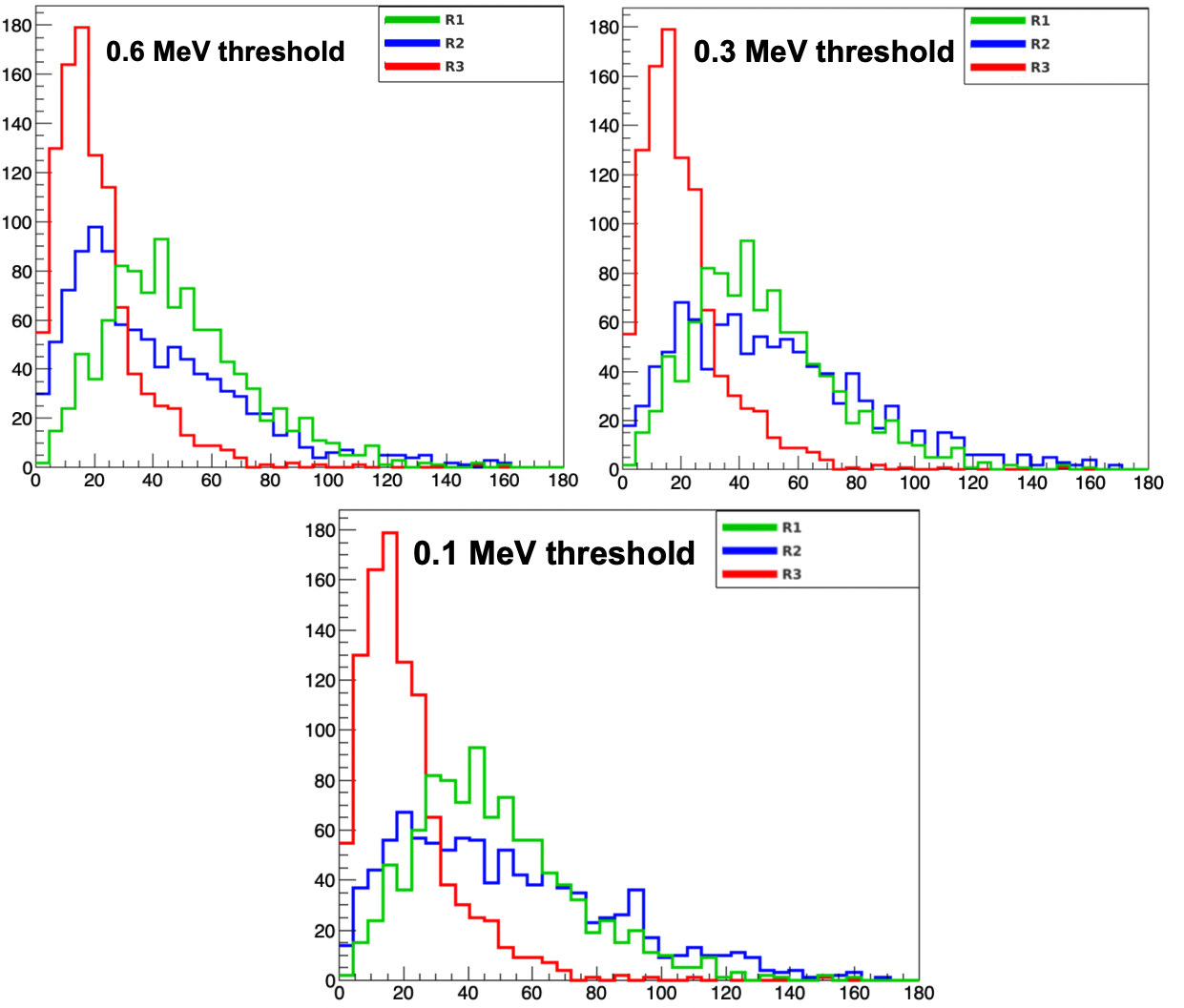

To compare the influence of the background and the low-energy threshold, we examine the final neutrino direction reconstruction result, shown in Fig. 35. Under the background assumptions discussed previously, lowering the energy threshold to 0.3 and 0.1 MeV significantly smears the original neutrino reconstruction distribution. The distribution that includes the neutron momentum reconstruction retains the same peak but develops a longer tail as the threshold decreases. This can be explained by the same effect in the neutron direction reconstruction shown in Fig. 34.
The reconstruction results are presented in Fig. 36 across neutrino energy bins in the channel. The upper bound of the neutron-inclusive reconstruction is approximately consistent with the baseline, while the lower bound and the peak value remain below it. This behavior is in agreement with the 0.5 GeV reconstruction shown in Fig. 35, indicating a modest improvement in reconstruction performance even in the high-background regime.
References
- [1] (2026-01) Reconstruction of atmospheric neutrinos in DUNE’s horizontal-drift far-detector module. External Links: 2601.05697 Cited by: §I, §V.
- [2] (2018-04) Atmospheric neutrino oscillation analysis with external constraints in super-kamiokande i-iv. Phys. Rev. D 97, pp. 072001. External Links: Document, Link Cited by: §I.
- [3] (2025-01) First joint oscillation analysis of super-kamiokande atmospheric and t2k accelerator neutrino data. Phys. Rev. Lett. 134, pp. 011801. External Links: Document, Link Cited by: §I.
- [4] (2020) Deep Underground Neutrino Experiment (DUNE), Far Detector Technical Design Report, Volume II: DUNE Physics. External Links: 2002.03005, Link Cited by: §I.
- [5] (2022) Wire-cell 3D pattern recognition techniques for neutrino event reconstruction in large LArTPCs: algorithm description and quantitative evaluation with MicroBooNE simulation. JINST 17 (01), pp. P01037. External Links: 2110.13961, Document Cited by: §V.1.
- [6] (2024) Demonstration of neutron identification in neutrino interactions in the MicroBooNE liquid argon time projection chamber. Eur. Phys. J. C 84 (10), pp. 1052. External Links: 2406.10583, Document Cited by: §V.
- [7] (2024) DUNE Phase II: Scientific Opportunities, Detector Concepts, Technological Solutions. Vol. 19. External Links: 2408.12725, Link, Document Cited by: §III, §VI.
- [8] (2025) Neutrino interaction vertex reconstruction in DUNE with Pandora deep learning. Eur. Phys. J. C 85 (697), pp. 697. External Links: 2502.06637, Document Cited by: §V.1.
- [9] (2001-07) Measurement of the rate of interactions produced by solar neutrinos at the sudbury neutrino observatory. Phys. Rev. Lett. 87, pp. 071301. External Links: Document, Link Cited by: §I.
- [10] (2002-06) Direct evidence for neutrino flavor transformation from neutral-current interactions in the sudbury neutrino observatory. Phys. Rev. Lett. 89, pp. 011301. External Links: Document, Link Cited by: §I.
- [11] (2004-09) Evidence for an oscillatory signature in atmospheric neutrino oscillations. Phys. Rev. Lett. 93, pp. 101801. External Links: Document, Link Cited by: §I.
- [12] (2005-06) Measurement of atmospheric neutrino oscillation parameters by super-kamiokande i. Phys. Rev. D 71, pp. 112005. External Links: Document, Link Cited by: §I.
- [13] Liquid Argon Properties. External Links: Link Cited by: 2nd item.
- [14] (2026) DUNE Baseline Model and Uncertainties. External Links: Link Cited by: §II, §III.1.
- [15] (2020) Calorimetry for low-energy electrons using charge and light in liquid argon. Phys. Rev. D 101 (1), pp. 012010. External Links: 1909.07920, Document Cited by: 1st item.
- [16] (2019) Understanding the energy resolution of liquid argon neutrino detectors. Phys. Rev. D 99 (3), pp. 036009. External Links: 1811.06159, Document Cited by: §V.
- [17] (1998-08) Evidence for oscillation of atmospheric neutrinos. Phys. Rev. Lett. 81, pp. 1562–1567. External Links: Document, Link Cited by: §I.
- [18] (2023-02) Neutron detection and application with a novel 3d-projection scintillator tracker in the future long-baseline neutrino oscillation experiments. Phys. Rev. D 107, pp. 032012. External Links: Document, Link Cited by: §I.
- [19] (2025-04) Measurements of pion and muon nuclear capture at rest on argon in the lariat experiment. Phys. Rev. Lett. 134, pp. 131801. External Links: Document, Link Cited by: §IV.
- [20] (2019-08) Sub-gev atmospheric neutrinos and violation in dune. Phys. Rev. Lett. 123, pp. 081801. External Links: Document, Link Cited by: §I, §V.
- [21] (2026-04) Neutron Reconstruction via Blips in Liquid Argon Time Projection Chambers. External Links: 2604.11774 Cited by: §I, §IV, 1st item, 2nd item, §VI, §VI, §VI, §VI.
- [22] (2025-02) Self-compensating light calorimetry with liquid argon time projection chamber for gev neutrino physics. Phys. Rev. D 111, pp. 032007. External Links: Document, Link Cited by: §I, §II, Figure 10, §III.1, §III.1, §III.1, §III.1, §III.2, §III.2, §III.3, §III.3, §III.3, §III.3, §III, §VII.
- [23] (2025-12) Modeling Light Signals Using Data from the First Pulsed Neutron Source Program at the DUNE Vertical Drift ColdBox Test Facility at CERN Neutrino Platform. External Links: 2512.10790 Cited by: §VII.
- [24] (2011) Scikit-learn: machine learning in Python. Journal of Machine Learning Research 12, pp. 2825–2830. Cited by: §IV.2.
- [25] (2025-07) Physics prospects with mev neutrino-argon charged current interactions using enhanced photon detection in future lartpcs. Phys. Rev. D 112, pp. 012019. External Links: Document, Link Cited by: §I, §II, §III.1, §III.
- [26] (2024-04) Atmospheric neutrino oscillation analysis with neutron tagging and an expanded fiducial volume in super-kamiokande i–v. Phys. Rev. D 109, pp. 072014. External Links: Document, Link Cited by: §I.