Transient Stability of Nonlinear Stochastic Dynamics: A Finite-Amplitude Logarithmic Measure Framework
Abstract
Spacecraft guidance, navigation, and control systems operating during mission-critical phases such as atmospheric entry, powered descent, and planetary landing require reliable assessment of finite-time transient behavior under stochastic uncertainty. Existing stochastic stability frameworks primarily characterize asymptotic or infinitesimal behavior and therefore provide limited insight into finite-amplitude transient amplification over operationally relevant time horizons.
This paper develops a finite-amplitude logarithmic measure for nonlinear Itô stochastic differential equations, extending classical matrix measures from infinitesimal to finite-amplitude perturbation evolution. The proposed framework establishes finite-time mean and variance bounds for logarithmic perturbation growth, derives Chernoff-type probabilistic bounds on transient amplification, and shows that mean transient stability does not necessarily guarantee finite-time pathwise safety. The theory is further extended to projected stochastic dynamics, leading to a transient-risk index that quantitatively balances deterministic contraction and diffusion-induced variability for transient-risk-aware system design.
The proposed framework is validated through Monte Carlo simulations and flight-like lunar descent telemetry. The results demonstrate substantially improved prediction of nonlinear transient growth compared with classical Jacobian-based approaches and successfully distinguish trajectories exhibiting similar nominal behavior but significantly different transient-risk characteristics. The proposed framework provides a unified methodology for finite-time transient stability analysis, probabilistic transient-risk assessment, and transient-risk-aware guidance, navigation, and control of nonlinear stochastic aerospace systems.
keywords:
Transient stability , Nonlinear stochastic systems , Finite-amplitude logarithmic measure , Finite-time analysis , Spacecraft navigation , Lunar descent[ursc] organization=U R Rao Satellite Centre, Indian Space Research Organisation (ISRO), city=Bengaluru, postcode=560017, country=India
[iisc] organization=Centre for Computational and Data Sciences, Indian Institute of Science, city=Bengaluru, postcode=560012, country=India
Introduces a finite-amplitude logarithmic measure for nonlinear Itô stochastic systems.
Develops deterministic and probabilistic finite-time transient stability theory.
Extends transient stability analysis to projected stochastic dynamics.
Proposes a transient-risk index for transient-risk-aware system design.
Validates the framework using Monte Carlo simulations and flight-like lunar descent telemetry.
1 Introduction
Spacecraft guidance, navigation, and control (GNC) systems operate under significant uncertainty during mission-critical operations such as atmospheric entry, powered descent, planetary landing, rendezvous, and autonomous docking. During these phases, small state perturbations may undergo substantial transient amplification over short time horizons, producing safety-critical deviations before asymptotic stability mechanisms become dominant. Quantifying finite-time stochastic perturbation growth is therefore fundamental for the design of robust autonomous guidance, navigation, and control algorithms for future space missions.
Classical stochastic stability theory has primarily focused on asymptotic, exponential, or moment-based notions of stability, typically established through Lyapunov methods, martingale techniques, or second-moment estimates [17, 4, 11]. Although mathematically well established these approaches primarily characterize asymptotic behavior and provide limited insight into finite-time transient perturbation growth.
Finite-time and fixed-time stabilization have been extensively studied for deterministic and stochastic systems [12, 19, 27, 28]. However, these frameworks address convergence properties rather than finite-time perturbation amplification in nonlinear continuous-time Itô systems.
A complementary perspective is provided by incremental stability and contraction theory [3, 14, 8, 18, 16, 5, 9, 10, 2, 13], which characterize trajectory-wise perturbation dynamics. Related studies on non-normal systems [25, 22] demonstrate that substantial transient amplification may occur despite asymptotic stability. However, these approaches remain fundamentally based on infinitesimal perturbations and do not characterize finite-amplitude nonlinear transient growth.
Existing stochastic logarithmic norm formulations [1, 2] are effective for linear and weakly nonlinear systems. Extending them to computationally tractable finite-time transient analysis of strongly nonlinear Itô stochastic systems without Jacobian linearization remains an open problem.
These limitations are particularly important in projection-based navigation and estimation systems, where continuous data assimilation modifies both the system dynamics and transient stability properties [6, 23, 24, 7, 20]. Similar challenges arise in atmospheric entry, powered-descent guidance, and planetary landing systems operating under significant uncertainty, where robust guidance and trajectory optimization are essential for reliable mission performance [15, 21, 26].
To address these challenges, this paper develops a unified finite-amplitude transient stability framework for nonlinear Itô stochastic systems, establishing deterministic and probabilistic finite-time transient bounds, extending the analysis to projected dynamics, and introducing a transient-risk index for risk-aware design.
The principal contributions are summarized as follows.
-
1.
Finite-amplitude logarithmic measure. A logarithmic measure for nonlinear Itô stochastic differential equations extending classical matrix measures from infinitesimal to finite-amplitude perturbation evolution.
-
2.
Unified finite-time transient stability theory. Finite-time mean, variance, and probabilistic transient-growth bounds together with a transient-risk index unifying deterministic contraction and diffusion-induced variability.
-
3.
Projected stochastic dynamics. Extension to projected stochastic dynamics with transient-risk-aware design, validated through Monte Carlo simulations and flight-like lunar descent telemetry.
Figure 1 summarizes the proposed computational pipeline.

2 Preliminaries and Problem Statement
This section introduces the stochastic dynamical model, finite-perturbation formulation, and transient-stability problem underlying the proposed framework.
2.1 Notation and Probability Space
Let be a complete probability space equipped with a right-continuous filtration . Expectations and variances are denoted by and , respectively. For , denotes the norm, with denoting the Euclidean norm when no ambiguity arises. The identity matrix is denoted by .
2.2 Stochastic Differential Equation
We consider nonlinear Itô stochastic differential equations of the form
| (1) |
where is the system state, is the drift field, are diffusion fields, and are independent Wiener processes. Throughout, stochastic integrals are interpreted in the Itô sense, and all processes are assumed adapted to [17].
Assumption 2.1.
The drift and diffusion mappings and , , are locally Lipschitz in and satisfy the linear growth condition
| (2) |
for some constant .
2.3 Perturbation Dynamics
To characterize finite-time transient behavior, we consider finite perturbations evolving under the same realization of the driving Wiener process. Let denote a non-zero finite perturbation of the state trajectory along a given sample path. The corresponding perturbation dynamics are defined as
| (3) |
where
| (4) |
Equation (3) defines the exact nonlinear perturbation dynamics without Jacobian linearization or variational equations.
Since perturbation amplification is inherently multiplicative, transient growth is characterized through the logarithm of the perturbation norm.
Definition 2.2 (Transient Stability).
Let denote the perturbation process associated with (1). The system is said to be
-
1.
mean transiently stable on if
for all sufficiently small and all ;
-
2.
pathwise transiently stable with confidence level on if
The objective of this paper is to characterize finite-time perturbation growth on nonlinear stochastic flows through a finite-amplitude logarithmic measure. To this end, we derive deterministic and probabilistic finite-time bounds for , which form the basis for the subsequent theoretical developments.
3 Logarithmic Norm in the Lipschitz Sense
This section introduces a finite-amplitude logarithmic measure for nonlinear mappings that extends classical matrix measures from infinitesimal to finite perturbation evolution.
3.1 Definition
Let be locally Lipschitz. For any finite perturbation , define
Definition 3.1 (Logarithmic Norm Induced by the -Norm).
| (5) |
Unlike the classical matrix measure, Definition 3.1 is formulated directly on finite perturbation increments.
Theorem 3.2 (Well-Posedness).
Let be locally Lipschitz on an open set . Then the logarithmic measure defined by (5) is well defined and finite.
Proof.
Since is locally Lipschitz,
The reverse triangle inequality gives
so the upper Dini derivative in Definition 3.1 is finite. ∎
An equivalent representation is
| (6) |
whenever the induced Lipschitz constant is well defined. This is the nonlinear analogue of the classical matrix-measure formula.
Theorem 3.3 (Consistency with Classical Matrix Measures).
Suppose for some matrix . Then the nonlinear logarithmic measure defined by (5) coincides with the classical logarithmic norm,
Proof.
Theorem 3.4 (Local Jacobian Representation).
Assume that is continuously differentiable. Then
Consequently,
in the infinitesimal perturbation limit.
Proof.
The first-order Taylor expansion gives
Substituting into Definition 3.1 and letting recovers the classical Jacobian logarithmic measure. ∎
Proposition 3.5 (Finite-Amplitude Deviation).
Assume that . Then, for finite perturbations,
Proof.
The second-order Taylor expansion gives
Substituting into Definition 3.1 yields
which proves the result. ∎
3.2 First-Order Characterization
A first-order expansion in the upper Dini derivative sense admits the representation
| (7) |
or, equivalently,
| (8) |
where
| (9) |
We denote this gradient by
3.3 Gradient and Hessian Properties
Let
The gradient of is given by
| (10) |
The Hessian exists almost everywhere for and is given componentwise by
| (11) | ||||
where denotes the Kronecker delta.
Equivalently,
| (12) |
where is defined in (10).
Lemma 3.6 (Hessian Bound).
There exists a constant depending only on the norm parameter such that
| (13) |
Proof.
Equation (12) shows that every Hessian term scales as . Norm equivalence in finite-dimensional spaces then yields
for some constant . ∎
3.4 Structural Properties
Proposition 3.7 (Subadditivity).
For any locally Lipschitz mappings and , the logarithmic norm satisfies the conservative bound
| (14) |
where denotes the -Lipschitz constant of .
Proof.
From Definition (5),
Using the triangle inequality,
Hence,
Using Lipschitz continuity of , which yields the result. ∎
Proposition 3.8 (Positive Homogeneity).
For every scalar ,
Proof.
Proposition 3.9 (Logarithmic Norm Upper Bound).
If the nonlinear mapping is Lipschitz continuous with respect to the -norm with Lipschitz constant , then
| (15) |
Proof.
By Lipschitz continuity,
Using Definition (5) together with the triangle inequality,
Dividing by and taking yields
∎
4 Transient Growth of Stochastic Perturbations
This section develops the finite-time transient stability theory underlying the proposed framework. Building upon the finite-amplitude logarithmic measure of Section 3, we derive explicit mean and variance bounds for logarithmic perturbation growth, forming the basis for the probabilistic analysis in Section 5.
4.1 Perturbation Dynamics and Logarithmic Growth
Applying Itô’s formula to the logarithmic perturbation norm yields
| (16) |
4.2 Mean Transient Growth Bound
Taking expectations in (16) eliminates the martingale term and yields the following upper bound on the expected logarithmic perturbation growth rate.
Theorem 4.1 (Mean Transient Growth Bound).
Assume that each diffusion field is locally Lipschitz with constant . Then
| (17) |
where
and is the constant introduced in Lemma 3.6.
Proof.
Applying Itô’s formula to and taking expectations eliminates the martingale term, yielding
Corollary 4.2 (Sufficient Mean Stability Condition).
If
| (18) |
then
Consequently, the expected logarithmic perturbation norm is non-increasing over finite time intervals.
4.3 Variance Bound
The following proposition bounds the diffusion-induced variability of logarithmic perturbation growth.
Proposition 4.3 (Variance Bound).
The infinitesimal variance growth of the logarithmic perturbation norm satisfies
| (19) |
where depends only on the chosen norm.
Proof.
Theorem 4.4 (Finite-Time Transient Stability Decomposition).
| (21) |
Proof.
The quantities and provide first- and second-moment characterizations of finite-time logarithmic perturbation growth and form the basis for the probabilistic analysis in the next section.
5 Probabilistic Transient Stability Bounds
This section derives finite-time probabilistic bounds on transient amplification by combining the mean and variance bounds of Section 4 with exponential concentration arguments.
Define the logarithmic perturbation increment
over the interval .
For sufficiently small , Theorem 4.1 and Proposition 4.3 imply
| (22) | ||||
| (23) |
where and are defined in Theorem 4.4.
5.1 Chernoff Bound
For any , Chernoff’s inequality yields
| (24) |
For sufficiently small , a second-order cumulant expansion yields
| (25) |
as .
Therefore,
| (27) |
For , the bound is minimized by choosing
Substituting the optimal Chernoff parameter gives
| (28) |
Equation (28) shows that the probability of transient amplification decays exponentially as deterministic contraction increasingly dominates diffusion-induced variability. Consequently, naturally emerges as the transient-risk index.
5.2 Pathwise Safety
Equation (28) shows that mean transient stability does not guarantee finite-time pathwise safety. Although the expected logarithmic growth rate may be negative, diffusion-induced variability permits transient amplification with nonzero probability over finite time horizons.
Collectively, these results characterize finite-time transient amplification through the deterministic growth-rate bound and stochastic variability bound , forming the basis for the transient-risk framework developed in Section 7.
6 Data-Constrained and Projected Stochastic Dynamics
This section extends the proposed framework to projection-based stochastic systems.
6.1 Projected Stochastic Dynamics
Many estimation and navigation algorithms incorporate continuous measurement updates or constraint enforcement. We consider the projected stochastic dynamics Let denote a continuously differentiable observation or constraint function, with Jacobian Assume that is invertible for all of interest. Define the projection operator
| (29) |
Remark 6.1.
Consider the projected stochastic differential equation
| (30) |
where denotes observed data and is a standard Wiener process.
6.2 Perturbation Dynamics under Projection
Let denote a finite perturbation of (30). The corresponding perturbation dynamics are given by
| (31) |
where all derivatives are evaluated along the sample path . Here, denotes the finite-difference increment of the composite mapping , interpreted in the Lipschitz sense introduced in Section 3.
The observation noise is assumed independent of the process noise, and perturbations are interpreted in the finite-difference sense.
6.3 Logarithmic Norm Bound under Projection
Applying the transient-growth analysis of Sections 3–5 to the composite mapping
yields the following bound.
Theorem 6.2 (Projected Transient Growth Bound).
The expected logarithmic perturbation growth rate satisfies the bound
| (32) |
where is the data-injection operator, its th column, and the observation mean rate interpreted in the weak (distributional) sense.
Proof.
Define the projected transient-growth parameter
6.4 Impact of Data Injection on Transient Stability
Proposition 6.3 (Data-Induced Variance Growth).
The infinitesimal variance growth of the logarithmic perturbation norm satisfies
| (33) |
where denotes the Lipschitz constant of the th column of the data-injection operator .
Proof.
The projected diffusion-variability parameter
Theorem 6.4 (Projected Transient Stability).
The finite-time transient behavior of the projected stochastic system is characterized by the pair .
These results extend the proposed transient-stability framework to projection-based stochastic systems and provide the basis for the numerical validation in the next section.
7 Design Implications for Transient-Risk-Aware Systems
7.1 Transient-Risk Index
The probabilistic analysis of Section 5 shows that finite-time transient amplification is governed by the ratio . This observation motivates the definition of the transient-risk index
| (34) |
whenever .
Proposition 7.1 (Monotonicity of the Transient-Risk Index).
Proof.
The result follows immediately from (28), since the exponential function is strictly increasing and implies
∎
Proposition 7.1 shows that larger correspond to smaller theoretical upper bounds on finite-time transient amplification, making a natural design objective.
7.2 Design Optimization
The transient-risk index provides a natural objective for finite-time robust design by explicitly balancing deterministic contraction and diffusion-induced variability,
subject to mission or system constraints. Maximizing minimizes the theoretical upper bound on finite-time transient amplification while balancing deterministic contraction and diffusion-induced variability.
Optimization variables may include guidance and control gains, navigation filter parameters, trajectory design variables, sensor configurations, projection operators, and data-assimilation strategies. The transient-risk index therefore extends the framework from transient analysis to transient-risk-aware design.
7.3 Extension to Projected Systems
The projected transient stability theory of Section 6 extends the transient-risk formulation to continuously corrected stochastic systems. Replacing the unconstrained parameters and by their projected counterparts, yields the projected transient-risk index
which quantifies finite-time transient robustness under continuous measurement updates and projection operations. This provides a principled basis for designing projection operators and data-assimilation strategies that balance estimation performance and transient robustness.
More generally, the proposed framework applies to nonlinear stochastic systems satisfying the assumptions of Sections 2– 6, independent of the application domain. Representative applications include spacecraft guidance, navigation, and control, powered-descent guidance, planetary landing, nonlinear state estimation, autonomous rendezvous and docking, formation flying, and other safety-critical autonomous aerospace systems.
The transient-risk index also provides a quantitative criterion for autonomous guidance and decision making. When multiple feasible actions are available, candidate strategies can be ranked according to their transient-risk indices together with conventional performance measures such as fuel consumption, flight time, landing accuracy, mission safety. This enables transient-risk-aware guidance and trajectory selection by favoring actions with lower theoretical probabilities of finite-time transient amplification while satisfying conventional mission performance objectives.
8 Discussion and Aerospace Design Implications
The proposed finite-amplitude transient stability framework extends classical stochastic stability analysis from asymptotic and infinitesimal perturbation behavior to finite-time transient amplification in nonlinear stochastic systems. The theoretical developments together with the numerical and telemetry validation provide several insights for aerospace guidance, navigation, and control systems operating under stochastic uncertainty.
8.1 Implications for Aerospace Guidance and Navigation
Mission-critical aerospace guidance, navigation, and control operations, including atmospheric entry, powered descent, planetary landing, rendezvous, and autonomous docking, require reliable operation over finite time horizons in the presence of uncertainty. Although conventional stability analyses ensure asymptotic or local convergence, significant transient perturbation growth may still occur before asymptotic behavior dominates. Such transient amplification can degrade navigation accuracy, increase guidance errors, and reduce mission robustness during safety-critical operations.
Modern aerospace navigation systems continuously fuse measurements from inertial sensors, vision systems, terrain-relative navigation, GNSS (where available), and other onboard sensors. These measurement updates modify both deterministic contraction properties and diffusion-induced variability. Consequently, projection and data-assimilation strategies directly influence finite-time transient robustness.
The proposed framework provides a quantitative characterization of short-horizon transient behavior through finite-amplitude perturbation evolution, thereby complementing classical Lyapunov- and Jacobian-based analyses with information that is directly relevant to operational decision making.
8.2 Engineering Design Implications
The analytical results naturally suggest several practical design principles for stochastic autonomous aerospace systems.
-
1.
maximize deterministic contraction by reducing the transient-growth parameter ;
-
2.
reduce diffusion-induced variability by minimizing the variance parameter through improved sensing, estimation, and data-assimilation strategies;
-
3.
design projection operators that improve measurement consistency while limiting transient amplification;
-
4.
monitor empirical transient-growth and diffusion-variability indicators online to support transient-risk-aware supervision and fault detection.
These principles provide a quantitative basis for designing guidance, navigation, estimation, and control algorithms that explicitly account for finite-time robustness in addition to conventional asymptotic stability.
8.3 Relation to Existing Stability Frameworks
The proposed methodology complements existing Lyapunov, incremental stability, and contraction theories by explicitly characterizing finite-amplitude transient amplification over finite operational horizons.
Whereas classical approaches primarily quantify asymptotic convergence or infinitesimal perturbation behavior, the present framework directly evaluates finite-amplitude perturbation evolution, providing additional insight into short-term robustness under stochastic uncertainty.
Rather than replacing existing stability tools, the proposed methodology provides an additional analytical tool for evaluating transient robustness in nonlinear stochastic systems.
8.4 Illustrative Extension to Autonomous Spacecraft Guidance
Consider an autonomous spacecraft performing powered descent or planetary landing. Let denote the set of feasible guidance trajectories generated by an onboard guidance algorithm.
The stochastic dynamics associated with each candidate trajectory are represented by the nonlinear Itô model introduced in Section 2, where the drift and diffusion fields depend on spacecraft dynamics, terrain uncertainty, sensing geometry, and environmental disturbances.
Applying the proposed framework yields the transient-growth parameter , the diffusion-variability parameter , and the corresponding transient-risk index
Candidate trajectories can therefore be ranked using their transient-risk indices together with conventional mission objectives such as fuel consumption, flight time, and landing accuracy. Consequently, the proposed framework provides a quantitative basis for transient-risk-aware guidance and trajectory selection in future autonomous spacecraft missions.
9 Monte-Carlo Validation of Finite-Amplitude Transient-Growth Prediction
This section validates the proposed finite-amplitude logarithmic measure using Monte Carlo realizations by comparing its transient-growth prediction with the classical Jacobian logarithmic measure. The benchmark nonlinear system is
| (35) | ||||
which exhibits strong nonlinear transient amplification and therefore provides a challenging benchmark. For each realization, the initial condition was sampled uniformly from with finite perturbation . The nominal and perturbed trajectories were propagated over using MATLAB ode45 (RelTol , AbsTol ) with a fixed random seed.
For each realization, the true logarithmic perturbation growth rate was computed as
| (36) |
where .
The true growth rate was compared with
-
1.
the classical Jacobian logarithmic norm ;
-
2.
the proposed finite-amplitude logarithmic measure .
Prediction accuracy was quantified using the root mean square error
| (37) |
and the Pearson correlation coefficient between the predicted and true growth rates.
Statistical significance was assessed using a paired Wilcoxon signed-rank test.
9.1 Monte Carlo Statistical Validation
Across all Monte Carlo realizations, the proposed finite-amplitude logarithmic measure achieved lower prediction error than the classical Jacobian approximation in every realization. A paired Wilcoxon signed-rank test rejected equal predictive performance (), confirming that the observed improvement is statistically significant. These results demonstrate that directly evaluating finite-amplitude perturbation evolution provides substantially more accurate prediction of transient growth than classical Jacobian linearization, particularly when nonlinear interactions dominate the system dynamics.

Figure 2 shows that the proposed measure closely tracks the observed transient-growth rate, whereas the Jacobian approximation exhibits systematic prediction bias.


9.2 Summary of Quantitative Performance
Table 1 summarizes the quantitative performance of the proposed and classical logarithmic measures over Monte Carlo realizations.
| Metric | Jacobian | Proposed |
|---|---|---|
| Median RMSE | 0.5977 | 0.00310 |
| Mean RMSE | 3.292 | |
| Mean MAE | 234.518 | 0.0791 |
| Mean Maximum Error | 153.635 | |
| Median Spearman Correlation | 0.762 | |
| Mean Spearman Correlation | 0.032 | 0.769 |
| Mean Pearson Correlation | 0.424 | 0.990 |
| Mean RMSE Reduction | 99.97% | |
| Wilcoxon Signed-Rank -value | ||
Across 1000 Monte Carlo realizations, the proposed finite-amplitude logarithmic measure reduced the mean RMSE by 99.97% and significantly outperformed the classical Jacobian approximation (), providing strong numerical evidence supporting the proposed finite-amplitude transient-growth framework.




10 Experimental Validation Using Flight-Like Lunar Descent Telemetry
This section experimentally evaluates the proposed finite-amplitude transient stability framework using flight-like lunar descent telemetry. The objective is to determine whether the telemetry-derived transient indicators consistently distinguish successful and failed landing trajectories and provide experimental support for the theoretical predictions developed in Sections 3–6.
10.1 Flight Telemetry and Validation Objective
To establish empirical counterparts of the theoretical quantities developed in Sections 3–6, the following telemetry-derived observables are constructed directly from the recorded descent trajectories.
-
1.
Logarithmic perturbation norm which characterizes the evolution of finite-amplitude perturbations.
-
2.
Empirical transient-growth indicator
which estimates the instantaneous logarithmic perturbation growth rate.
-
3.
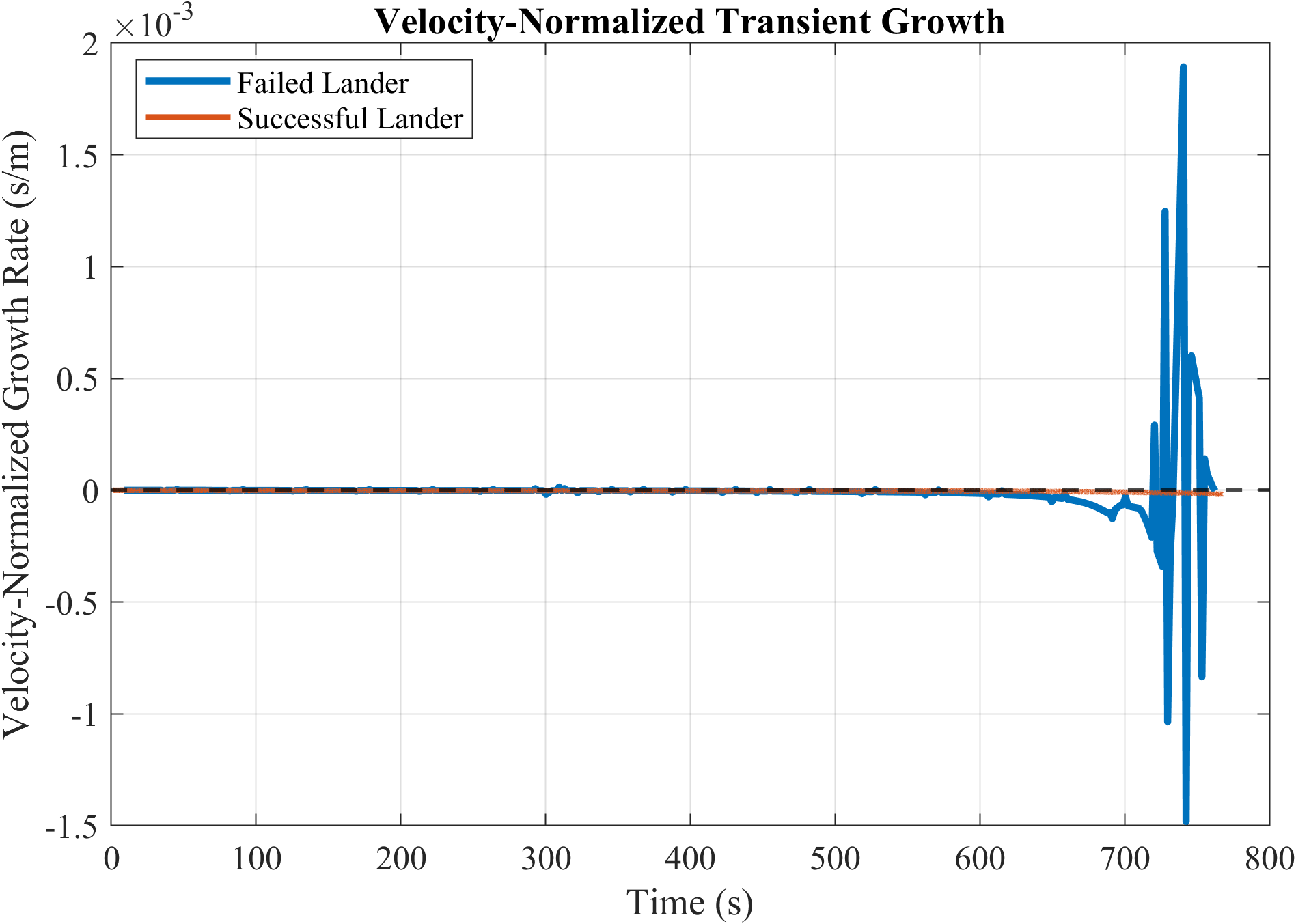
Velocity-normalized transient-growth indicator, used to distinguish intrinsic transient instability from variations caused by changing descent velocity.
-
4.
Diffusion-variability indicator , computed as a local estimate of the variance of logarithmic perturbation increments over a moving time window. This observable provides a data-driven estimate of diffusion-induced variability consistent with the variance term appearing in the Itô-based transient stability formulation.
-
5.
Frequency of transient instability events, defined by the fraction of time for which
-
6.
Cumulative transient instability,
which quantifies the accumulated exposure to finite-time transient amplification.
Remark 10.1.
The quantities and used in this section are empirical estimates of the instantaneous transient-growth rate and diffusion-induced variability, respectively. They serve as observable counterparts of the theoretical coefficients and introduced in Sections 4–5, but are not identical to the analytical bounds defined in (20) and (21).
10.2 Perturbation Growth and Transient Indicators
Figures 6 and 7 collectively illustrate the relationship between finite perturbation evolution and the corresponding empirical transient-growth indicator.
The logarithmic perturbation norm shown in Fig. 6 remains well behaved throughout the successful descent, whereas the failed trajectory exhibits localized perturbation amplification during the terminal descent phase. This amplification is accompanied by pronounced positive excursions of the empirical transient-growth indicator (Fig. 7) over –, indicating intervals of finite-time transient instability.
The coincidence of perturbation amplification and positive values of the empirical transient-growth indicator is consistent with the theoretical prediction that finite-time transient instability is associated with localized perturbation growth.
10.3 Diffusion Variability and Intrinsic Instability
Figures 8 and 11 together show that the transient instability observed during the failed descent is an intrinsic property of the underlying dynamics rather than a consequence of nominal trajectory variations.
The diffusion-variability indicator (Fig. 11) remains negligible throughout the successful descent but increases markedly during the terminal phase of the failed trajectory, consistent with the predicted increase in diffusion-induced variability accompanying finite-time transient instability. A smaller rise around coincides with a documented guidance–engine interaction anomaly, indicating that the proposed observable is sensitive to localized dynamical inconsistencies before mission failure.
Figure 8 further shows that the terminal excursions of the empirical transient-growth indicator persist after normalization by descent velocity. Thus, the observed transient amplification cannot be explained solely by nominal descent-rate variations but reflects the underlying nonlinear dynamics. Collectively, these observations indicate that finite-time transient instability is accompanied by simultaneous increases in empirical transient-growth rate and diffusion-induced variability.
10.4 Persistence and Accumulation of Transient Instability
Figures 9 and 10 characterize the temporal persistence of transient instability during descent through its occurrence frequency and cumulative accumulation.
Figure 9 shows that transient instability occurs more than twice as frequently in the failed trajectory as in the successful trajectory, whereas Fig. 10 shows that these events accumulate progressively during terminal descent, resulting in substantially greater cumulative instability exposure.
Collectively, these results indicate that mission outcome is more strongly associated with the persistence and cumulative accumulation of transient instability than with isolated transient-growth events.
10.5 Quantitative Validation and Engineering Implications
Table 2 summarizes the principal transient-stability metrics extracted from the flight-like lunar descent telemetry.
| Metric | Failed | Successful |
|---|---|---|
| Peak Growth Rate | 0.1374 | |
| Mean Growth Rate | -0.00349 | -0.00207 |
| Instability Frequency | 0.1073 | 0.0466 |
| Cumulative Instability | 1.5203 | 0.00068 |
| Peak Variability | 0.6559 |
The telemetry-derived transient-stability metrics consistently distinguish the successful and failed descent trajectories. Compared with the successful trajectory, the failed trajectory exhibits substantially larger transient-growth rates, diffusion-induced variability, instability frequency, and cumulative instability, indicating sustained finite-time perturbation amplification rather than isolated transient events.
Collectively, these results are consistent with the theoretical predictions developed throughout the paper and demonstrate that the proposed transient-stability metrics provide information beyond conventional trajectory-tracking and long-horizon stability measures. The derived indicators therefore provide a quantitative basis for assessing navigation robustness in autonomous aerospace systems.
Although demonstrated using flight-like lunar descent telemetry, the proposed methodology is applicable to a broad class of continuously differentiable nonlinear stochastic systems, including spacecraft guidance, navigation, and control, autonomous robotics, state estimation, autonomous vehicles, and other safety-critical engineering applications.
11 Conclusion
This paper developed a finite-amplitude logarithmic measure framework for finite-time transient stability analysis of nonlinear Itô stochastic differential equations. By extending classical logarithmic measures from infinitesimal Jacobian dynamics to finite-amplitude perturbation evolution, the proposed framework directly characterizes nonlinear transient growth on stochastic flows without requiring explicit variational equations or Lyapunov-function construction.
The resulting theory establishes deterministic and probabilistic finite-time transient stability through explicit bounds on the mean and variance of logarithmic perturbation growth together with Chernoff-type probabilistic bounds on transient amplification. The extension to projected stochastic dynamics further introduces a transient-risk index that unifies deterministic contraction and diffusion-induced variability, providing a computationally tractable framework for transient-risk-aware analysis and system design.
The proposed framework was validated through 1000 Monte Carlo simulations and flight-like lunar descent telemetry. The numerical and telemetry results demonstrate substantially improved prediction of nonlinear transient growth compared with the classical Jacobian logarithmic measure and show that trajectories exhibiting similar nominal behavior may possess markedly different finite-time transient-risk characteristics.
Overall, the proposed framework establishes a unified methodology for finite-time transient stability analysis, probabilistic transient-risk assessment, and transient-risk-aware design of nonlinear stochastic systems. Beyond its application to lunar descent telemetry, the framework is applicable to a broad class of autonomous aerospace systems, including spacecraft guidance, navigation, and control, planetary landing, rendezvous and docking, formation flying, and onboard state estimation under stochastic uncertainty.
Future work will investigate transient-risk-aware guidance and control, adaptive projection and data-assimilation strategies, stochastic observer design, and real-time onboard transient-risk monitoring for next-generation autonomous aerospace systems.
References
- [1] (2010) On estimation of transient stochastic stability of linear systems. Stochastics and Dynamics 10 (03), pp. 391–415. Cited by: §1.
- [2] (2022) Stochastic logarithmic lipschitz constants: a tool to analyze contractivity of stochastic differential equations. IEEE control systems letters 6, pp. 2311–2316. Cited by: §1, §1.
- [3] (2002) A lyapunov approach to incremental stability properties. Automatica 38 (6), pp. 1025–1032. External Links: Document Cited by: §1.
- [4] (1998) Random dynamical systems. Springer. Cited by: §1, §2.2.
- [5] (2008) Piecewise-smooth dynamical systems: theory and applications. Applied Mathematical Sciences 163. Cited by: §1.
- [6] (2010) Minimum-landing-error powered-descent guidance for mars landing using convex optimization. Journal of Guidance, Control, and Dynamics 33 (4), pp. 1161–1171. External Links: Document Cited by: §1.
- [7] (2012) Optimal estimation of dynamic systems. 2 edition, CRC Press. Cited by: §1, Remark 6.1.
- [8] (2014) A differential lyapunov framework for contraction analysis. Automatica 50 (3), pp. 614–628. External Links: Document Cited by: §1.
- [9] (2024) Contraction analysis of discrete-time stochastic systems. IEEE Transactions on Automatic Control 69, pp. 982–997. External Links: Document Cited by: §1.
- [10] (2025) Contraction Analysis of Differentially Positive Discrete-Time Stochastic Systems. IEEE Transactions on Automatic Control. External Links: Document Cited by: §1.
- [11] (2012) Stochastic stability of differential equations. 2 edition, Stochastic Modelling and Applied Probability, Vol. 66, Springer, Berlin, Heidelberg. External Links: Document, ISBN 978-3-642-23279-4 Cited by: §1.
- [12] (2022) Finite-time stability and optimal finite-time stabilization for discrete-time stochastic dynamical systems. IEEE Transactions on Automatic Control. External Links: Document Cited by: §1.
- [13] (2024) Incremental stability and contraction analysis for stochastic systems via matrix measures. Automatica 161, pp. 111450. Cited by: §1.
- [14] (1998) On contraction analysis for nonlinear systems. Automatica 34 (6), pp. 683–696. External Links: Document Cited by: §1.
- [15] (2018) Propellant-optimal powered descent guidance. Journal of Guidance, Control, and Dynamics 41 (4), pp. 813–826. External Links: Document Cited by: §1.
- [16] (2017) Control contraction metrics: convex and intrinsic criteria for nonlinear feedback design. IEEE Transactions on Automatic Control 62 (6), pp. 3046–3053. External Links: Document Cited by: §1.
- [17] (2007) Stochastic differential equations and applications. Woodhead Publishing. Cited by: §1, §2.2, §2.2.
- [18] (2008) Convergent systems: analysis and design. Automatica 44 (10), pp. 2457–2466. External Links: Document Cited by: §1.
- [19] (2012) Nonlinear feedback design for fixed-time stabilization of linear control systems. Automatica 48 (8), pp. 1409–1415. External Links: Document Cited by: §1.
- [20] (2015) Probabilistic forecasting and bayesian data assimilation. Cambridge University Press. Cited by: §1, Remark 6.1.
- [21] (2021) Optimal drag-energy entry guidance via pseudospectral convex optimization. Aerospace Science and Technology 117, pp. 106946. External Links: Document Cited by: §1.
- [22] (2007) Nonmodal stability theory. Annual Review of Fluid Mechanics 39, pp. 129–162. External Links: Document Cited by: §1.
- [23] (2021) Event-based spacecraft landing using time-to-contact. In IEEE/CVF Conference on Computer Vision and Pattern Recognition Workshops (CVPRW), pp. 1941–1950. External Links: Document Cited by: §1.
- [24] (2014) Stability analysis for stochastic hybrid systems: a survey. Automatica 50 (10), pp. 2435–2456. External Links: Document Cited by: §1.
- [25] (1993) Hydrodynamic stability without eigenvalues. Science 261 (5121), pp. 578–584. External Links: Document Cited by: §1.
- [26] (2022) Rocket landing guidance using convex optimization and proportional navigation considering performance-limited engine. Acta Astronautica 201, pp. 209–223. External Links: Document Cited by: §1.
- [27] (2022) Finite-time stability and stabilization of itô stochastic systems. IEEE Transactions on Aerospace and Electronic Systems 58 (5), pp. 4200–4212. External Links: Document Cited by: §1.
- [28] (2022) Fixed-time stability of stochastic nonlinear systems with applications. Automatica 140, pp. 110214. External Links: Document Cited by: §1.